Overview of the H.264 / AVC Video Coding Standard654lab.webstarts.com/uploads/csvt_overview.pdf · AVC, H.264, JVT. I. INTRODUCTION is the newest international video coding standard

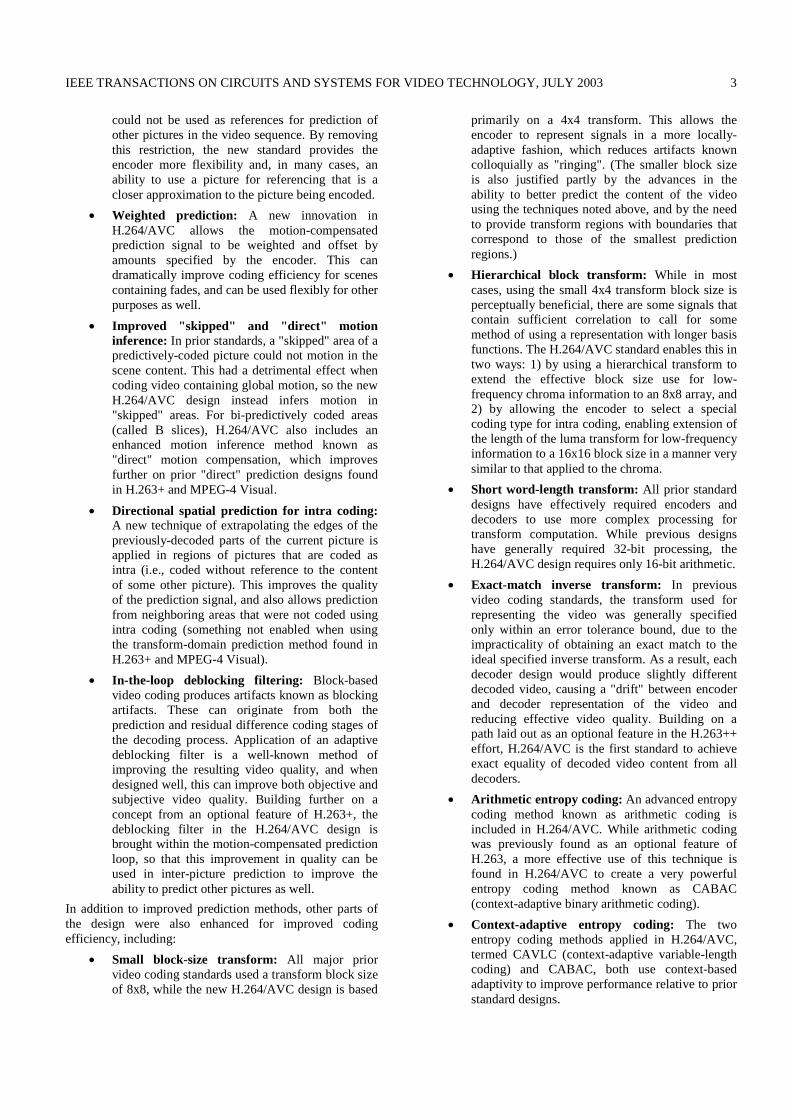
IEEE TRANSACTIONS ON CIRCUITS AND SYSTEMS FOR VIDEO TECHNOLOGY, JULY 2003 1

Abstract— H.264/AVC is newest video coding standard of the ITU-T Video Coding Experts Group (VCEG) and the ISO/IEC Moving Picture Experts Group (MPEG). The main goals of the H.264/AVC standardization effort have been enhanced compression performance and provision of a "network-friendly" video representation addressing "conversational" (video telephony) and "non-conversational" (storage, broadcast, or streaming) applications. H.264/AVC has achieved a significant improvement in rate-distortion efficiency relative to existing standards. This article provides an overview of the technical features of H.264/AVC, describes profiles and applications for the standard, and outlines the history of the standardization process.

Index Terms—Video, Standards, MPEG-2, H.263, MPEG-4, AVC, H.264, JVT.

I. INTRODUCTION

is the newest international video coding standard [1]. By the time of this publication, it

is expected to have been approved by ITU-T as Recommendation H.264 and by ISO/IEC as International Standard 14496-10 (MPEG-4 part 10) Advanced Video Coding (AVC).

The MPEG-2 video coding standard (also known as ITU-T H.262) [2], which was developed about 10 years ago primarily as an extension of prior MPEG-1 video capability with support of interlaced video coding, was an enabling technology for digital television systems worldwide. It is widely used for the transmission of standard definition (SD) and High Definition (HD) TV signals over satellite, cable, and terrestrial emission and the storage of high-quality SD video signals onto DVDs.

However, an increasing number of services and growing popularity of high definition TV are creating greater needs for higher coding efficiency. Moreover, other transmission media such as Cable Modem, xDSL or UMTS offer much lower data rates than broadcast channels, and enhanced coding efficiency can enable the transmission of more video channels or higher quality video representations within existing digital transmission capacities.

Video coding for telecommunication applications has evolved through the development of the ITU-T H.261, H.262 (MPEG-2), and H.263 video coding standards (and later enhancements of H.263 known as H.263+ and H.263++), and has diversified from ISDN and T1/E1

service to embrace PSTN, mobile wireless networks, and LAN/Internet network delivery. Throughout this evolution, continued efforts have been made to maximize coding efficiency while dealing with the diversification of network types and their characteristic formatting and loss/error robustness requirements.

Recently the MPEG-4 Visual (MPEG-4 part 2) standard [5] has also begun to emerge in use in some application domains of the prior coding standards. It has provided video shape coding capability, and has similarly worked toward broadening the range of environments for digital video use.

In early 1998 the Video Coding Experts Group (VCEG – ITU-T SG16 Q.6) issued a call for proposals on a project called H.26L, with the target to double the coding efficiency (which means halving the bit rate necessary for a given level of fidelity) in comparison to any other existing video coding standards for a broad variety of applications. The first draft design for that new standard was adopted in October of 1999. In December of 2001, VCEG and the Moving Picture Experts Group (MPEG – ISO/IEC JTC 1/SC 29/WG 11) formed a Joint Video Team (JVT), with the charter to finalize the draft new video coding standard for formal approval submission as H.264/AVC [1] in March 2003.

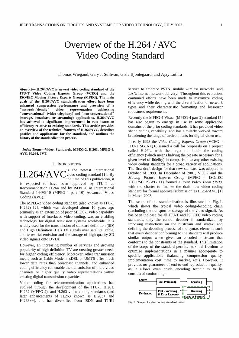
The scope of the standardization is illustrated in Fig. 1, which shows the typical video coding/decoding chain (excluding the transport or storage of the video signal). As has been the case for all ITU-T and ISO/IEC video coding standards, only the central decoder is standardized, by imposing restrictions on the bitstream and syntax, and defining the decoding process of the syntax elements such that every decoder conforming to the standard will produce similar output when given an encoded bitstream that conforms to the constraints of the standard. This limitation of the scope of the standard permits maximal freedom to optimize implementations in a manner appropriate to specific applications (balancing compression quality, implementation cost, time to market, etc.). However, it provides no guarantees of end-to-end reproduction quality, as it allows even crude encoding techniques to be considered conforming.

Pre -Processing EncodingSource

DestinationPost -Processing& Error Recovery

Decoding

Scope of Standard



Decoding

Scope of Standard



Decoding

Scope of Standard



Decoding

Scope of Standard Fig. 1: Scope of video coding standardization.

Overview of the H.264 / AVC Video Coding Standard

Thomas Wiegand, Gary J. Sullivan, Gisle Bjontegaard, and Ajay Luthra

H.264/AVC

WIEGAND et al.: OVERVIEW OF THE H.264/AVC VIDEO CODING STANDARD 2

This paper is organized as follows. Section II provides a high-level overview of H.264/AVC applications and highlights some key technical features of the design that enable improved operation for this broad variety of applications. Section III explains the network abstraction layer and the overall structure of H.264/AVC coded video data. The video coding layer is described in Section IV. Section V explains the profiles supported by H.264/AVC and some potential application areas of the standard.

II. APPLICATIONS AND DESIGN FEATURE HIGHLIGHTS

The new standard is designed for technical solutions including at least the following application areas

• Broadcast over cable, satellite, Cable Modem, DSL, terrestrial, etc.

• Interactive or serial storage on optical and magnetic devices, DVD, etc.

• Conversational services over ISDN, Ethernet, LAN, DSL, wireless and mobile networks, modems, etc. or mixtures of these.

• Video-on-demand or multimedia streaming services over ISDN, Cable Modem, DSL, LAN, wireless networks, etc.

• Multimedia Messaging Services (MMS) over ISDN, DSL, Ethernet, LAN, wireless and mobile networks, etc.

Moreover, new applications may be deployed over existing and future networks. This raises the question about how to handle this variety of applications and networks.

To address this need for flexibility and customizability, the H.264/AVC design covers a Video Coding Layer (VCL), which is designed to efficiently represent the video content, and a Network Abstraction Layer (NAL), which formats the VCL representation of the video and provides header information in a manner appropriate for conveyance by a variety of transport layers or storage media (see Fig. 2).

Video Coding Layer

Data Partitioning

Network Abstraction Layer

H.320 MP4FF H.323/IP MPEG-2 etc.

Con

trol

Dat

a

Coded Macroblock

Coded Slice/Partition

Video Coding Layer

Data Partitioning

Network Abstraction Layer

H.320 MP4FF H.323/IP MPEG-2 etc.

Con

trol

Dat

a

Coded Macroblock

Coded Slice/Partition

Fig. 2: Structure of H.264/AVC video encoder.

Relative to prior video coding methods, as exemplified by MPEG-2 video, some highlighted features of the design that enable enhanced coding efficiency include the following enhancements of the ability to predict the values of the content of a picture to be encoded:

• Variable block-size motion compensation with small block sizes: This standard supports more flexibility in the selection of motion compensation block sizes and shapes than any previous standard, with a minimum luma motion compensation block size as small as 4x4.

• Quarter-sample-accurate motion compensation: Most prior standards enable half-sample motion vector accuracy at most. The new design improves up on this by adding quarter-sample motion vector accuracy, as first found in an advanced profile of the MPEG-4 Visual (part 2) standard, but further reduces the complexity of the interpolation processing compared to the prior design.

• Motion vectors over picture boundaries: While motion vectors in MPEG-2 and its predecessors were required to point only to areas within the previously-decoded reference picture, the picture boundary extrapolation technique first found as an optional feature in H.263 is included in H.264/AVC.

• Multiple reference picture motion compensation: Predictively coded pictures (called "P" pictures) in MPEG-2 and its predecessors used only one previous picture to predict the values in an incoming picture. The new design extends upon the enhanced reference picture selection technique found in H.263++ to enable efficient coding by allowing an encoder to select, for motion compensation purposes, among a larger number of pictures that have been decoded and stored in the decoder. The same extension of referencing capability is also applied to motion-compensated bi-prediction, which is restricted in MPEG-2 to using two specific pictures only (one of these being the previous intra (I) or P picture in display order and the other being the next I or P picture in display order).

• Decoupling of referencing order from display order: In prior standards, there was a strict dependency between the ordering of pictures for motion compensation referencing purposes and the ordering of pictures for display purposes. In H.264/AVC, these restrictions are largely removed, allowing the encoder to choose the ordering of pictures for referencing and display purposes with a high degree of flexibility constrained only by a total memory capacity bound imposed to ensure decoding ability. Removal of the restriction also enables removing the extra delay previously associated with bi-predictive coding.

• Decoupling of picture representation methods from picture referencing capability: In prior standards, pictures encoded using some encoding methods (namely bi-predictively-encoded pictures)


could not be used as references for prediction of other pictures in the video sequence. By removing this restriction, the new standard provides the encoder more flexibility and, in many cases, an ability to use a picture for referencing that is a closer approximation to the picture being encoded.

• Weighted prediction: A new innovation in H.264/AVC allows the motion-compensated prediction signal to be weighted and offset by amounts specified by the encoder. This can dramatically improve coding efficiency for scenes containing fades, and can be used flexibly for other purposes as well.

• Improved "skipped" and "direct" motion inference: In prior standards, a "skipped" area of a predictively-coded picture could not motion in the scene content. This had a detrimental effect when coding video containing global motion, so the new H.264/AVC design instead infers motion in "skipped" areas. For bi-predictively coded areas (called B slices), H.264/AVC also includes an enhanced motion inference method known as "direct" motion compensation, which improves further on prior "direct" prediction designs found in H.263+ and MPEG-4 Visual.

• Directional spatial prediction for intra coding: A new technique of extrapolating the edges of the previously-decoded parts of the current picture is applied in regions of pictures that are coded as intra (i.e., coded without reference to the content of some other picture). This improves the quality of the prediction signal, and also allows prediction from neighboring areas that were not coded using intra coding (something not enabled when using the transform-domain prediction method found in H.263+ and MPEG-4 Visual).

• In-the-loop deblocking filtering: Block-based video coding produces artifacts known as blocking artifacts. These can originate from both the prediction and residual difference coding stages of the decoding process. Application of an adaptive deblocking filter is a well-known method of improving the resulting video quality, and when designed well, this can improve both objective and subjective video quality. Building further on a concept from an optional feature of H.263+, the deblocking filter in the H.264/AVC design is brought within the motion-compensated prediction loop, so that this improvement in quality can be used in inter-picture prediction to improve the ability to predict other pictures as well.

In addition to improved prediction methods, other parts of the design were also enhanced for improved coding efficiency, including:

• Small block-size transform: All major prior video coding standards used a transform block size of 8x8, while the new H.264/AVC design is based

primarily on a 4x4 transform. This allows the encoder to represent signals in a more locally-adaptive fashion, which reduces artifacts known colloquially as "ringing". (The smaller block size is also justified partly by the advances in the ability to better predict the content of the video using the techniques noted above, and by the need to provide transform regions with boundaries that correspond to those of the smallest prediction regions.)

• Hierarchical block transform: While in most cases, using the small 4x4 transform block size is perceptually beneficial, there are some signals that contain sufficient correlation to call for some method of using a representation with longer basis functions. The H.264/AVC standard enables this in two ways: 1) by using a hierarchical transform to extend the effective block size use for low-frequency chroma information to an 8x8 array, and 2) by allowing the encoder to select a special coding type for intra coding, enabling extension of the length of the luma transform for low-frequency information to a 16x16 block size in a manner very similar to that applied to the chroma.

• Short word-length transform: All prior standard designs have effectively required encoders and decoders to use more complex processing for transform computation. While previous designs have generally required 32-bit processing, the H.264/AVC design requires only 16-bit arithmetic.

• Exact-match inverse transform: In previous video coding standards, the transform used for representing the video was generally specified only within an error tolerance bound, due to the impracticality of obtaining an exact match to the ideal specified inverse transform. As a result, each decoder design would produce slightly different decoded video, causing a "drift" between encoder and decoder representation of the video and reducing effective video quality. Building on a path laid out as an optional feature in the H.263++ effort, H.264/AVC is the first standard to achieve exact equality of decoded video content from all decoders.

• Arithmetic entropy coding: An advanced entropy coding method known as arithmetic coding is included in H.264/AVC. While arithmetic coding was previously found as an optional feature of H.263, a more effective use of this technique is found in H.264/AVC to create a very powerful entropy coding method known as CABAC (context-adaptive binary arithmetic coding).

• Context-adaptive entropy coding: The two entropy coding methods applied in H.264/AVC, termed CAVLC (context-adaptive variable-length coding) and CABAC, both use context-based adaptivity to improve performance relative to prior standard designs.


Robustness to data errors/losses and flexibility for operation over a variety of network environments is enabled by a number of design aspects new to the H.264/AVC standard including the following highlighted features.

• Parameter set structure: The parameter set design provides for robust and efficient conveyance header information. As the loss of a few key bits of information (such as sequence header or picture header information) could have a severe negative impact on the decoding process when using prior standards, this key information was separated for handling in a more flexible and specialized manner in the H.264/AVC design.

• NAL unit syntax structure: Each syntax structure in H.264/AVC is placed into a logical data packet called a NAL unit. Rather than forcing a specific bitstream interface to the system as in prior video coding standards, the NAL unit syntax structure allows greater customization of the method of carrying the video content in a manner appropriate for each specific network.

• Flexible slice size: Unlike the rigid slice structure found in MPEG-2 (which reduces coding efficiency by increasing the quantity of header data and decreasing the effectiveness of prediction), slice sizes in H.264/AVC are highly flexible, as was the case earlier in MPEG-1.

• Flexible macroblock ordering (FMO): A new ability to partition the picture into regions called slice groups has been developed, with each slice becoming an independently-decodable subset of a slice group. When used effectively, flexible macroblock ordering can significantly enhance robustness to data losses by managing the spatial relationship between the regions that are coded in each slice. (FMO can also be used for a variety of other purposes as well.)

• Arbitrary slice ordering (ASO): Since each slice of a coded picture can be (approximately) decoded independently of the other slices of the picture, the H.264/AVC design enables sending and receiving the slices of the picture in any order relative to each other. This capability, first found in an optional part of H.263+, can improve end-to-end delay in real-time applications, particularly when used on networks having out-of-order delivery behavior (e.g., internet protocol networks).

• Redundant pictures: In order to enhance robustness to data loss, the H.264/AVC design contains a new ability to allow an encoder to send redundant representations of regions of pictures, enabling a (typically somewhat degraded) representation of regions of pictures for which the primary representation has been lost during data transmission.

• Data Partitioning: Since some coded information for representation of each region (e.g., motion

vectors and other prediction information) is more important or more valuable than other information for purposes of representing the video content, H.264/AVC allows the syntax of each slice to be separated into up to three different partitions for transmission, depending on a categorization of syntax elements. This part of the design builds further on a path taken in MPEG-4 Visual and in an optional part of H.263++. Here the design is simplified by having a single syntax with partitioning of that same syntax controlled by a specified categorization of syntax elements.

• SP/SI synchronization/switching pictures: The H.264/AVC design includes a new feature consisting of picture types that allow exact synchronization of the decoding process of some decoders with an ongoing video stream produced by other decoders without penalizing all decoders with the loss of efficiency resulting from sending an I picture. This can enable switching a decoder between representations of the video content that used different data rates, recovery from data losses or errors, as well as enabling trick modes such as fast-forward, fast-reverse, etc.

In the following two sections, a more detailed description of the key features is given.

III. NETWORK ABSTRACTION LAYER

The network abstraction layer (NAL) is designed in order to provide "network friendliness" to enable simple and effective customization of the use of the VCL for a broad variety of systems.

The NAL facilitates the ability to map H.264/AVC VCL data to transport layers such as

• RTP/IP for any kind of real-time wire-line and wireless Internet services (conversational and streaming)

• File formats, e.g. ISO MP4 for storage and MMS

• H.32X for wireline and wireless conversational services

• MPEG-2 systems for broadcasting services, etc.

The full degree of customization of the video content to fit the needs of each particular application is outside the scope of the H.264/AVC standardization effort, but the design of the NAL anticipates a variety of such mappings. Some key concepts of the NAL are NAL units, byte stream, and packet format uses of NAL units, parameter sets, and access units. A short description of these concepts is given below whereas a more detailed description including error resilience aspects is provided in [6] and [7].

A. NAL units

The coded video data is organized into NAL units, each of which is effectively a packet that contains an integer number of bytes. The first byte of each NAL unit is a header byte that contains an indication of the type of data in


the NAL unit, and the remaining bytes contain payload data of the type indicated by the header.

The payload data in the NAL unit is interleaved as necessary with emulation prevention bytes, which are bytes inserted with a specific value to prevent a particular pattern of data called a start code prefix from being accidentally generated inside the payload.

The NAL unit structure definition specifies a generic format for use in both packet-oriented and bitstream-oriented transport systems, and a series of NAL units generated by an encoder is referred to as a NAL unit stream.

B. NAL units in byte stream format use

Some systems (e.g., H.320 and MPEG-2 | H.222.0 systems) require delivery of the entire or partial NAL unit stream as an ordered stream of bytes or bits within which the locations of NAL unit boundaries need to be identifiable from patterns within the coded data itself.

For use in such systems, the H.264/AVC specification defines a byte stream format. In the byte stream format, each NAL unit is prefixed by a specific pattern of three bytes called a start code prefix. The boundaries of the NAL unit can then be identified by searching the coded data for the unique start code prefix pattern. The use of emulation prevention bytes guarantees that start code prefixes are unique identifiers of the start of a new NAL unit.

A small amount of additional data (one byte per video picture) is also added to allow decoders that operate in systems that provide streams of bits without alignment to byte boundaries to recover the necessary alignment from the data in the stream.

Additional data can also be inserted in the byte stream format that allows expansion of the amount of data to be sent and can aid in achieving more rapid byte alignment recovery, if desired.

C. NAL units in packet-transport system use

In other systems (e.g., internet protocol / RTP systems), the coded data is carried in packets that are framed by the system transport protocol, and identification of the boundaries of NAL units within the packets can be established without use of start code prefix patterns. In such systems, the inclusion of start code prefixes in the data would be a waste of data carrying capacity, so instead the NAL units can be carried in data packets without start code prefixes.

D. VCL and non-VCL NAL units

NAL units are classified into VCL and non-VCL NAL units. The VCL NAL units contain the data that represents the values of the samples in the video pictures, and the non-VCL NAL units contain any associated additional information such as parameter sets (important header data that can apply to a large number of VCL NAL units) and supplemental enhancement information (timing information and other supplemental data that may enhance usability of

the decoded video signal but are not necessary for decoding the values of the samples in the video pictures).

E. Parameter sets

A parameter set is supposed to contain information that is expected to rarely change and offers the decoding of a large number of VCL NAL units. There are two types of parameter sets:

• sequence parameter sets, which apply to a series of consecutive coded video pictures called a coded video sequence, and

• picture parameter sets, which apply to the decoding of one or more individual pictures within a coded video sequence.

The sequence and picture parameter set mechanism decouples the transmission of infrequently changing information from the transmission of coded representations of the values of the samples in the video pictures. Each VCL NAL unit contains an identifier that refers to the content of the relevant picture parameter set, and each picture parameter set contains an identifier that refers to the content of the relevant sequence parameter set. In this manner, a small amount of data (the identifier) can be used to refer to a larger amount of information (the parameter set) without repeating that information within each VCL NAL unit.

Sequence and picture parameter sets can be sent well ahead of the VCL NAL units that they apply to, and can be repeated to provide robustness against data loss. In some applications, parameter sets may be sent within the channel that carries the VCL NAL units (termed "in-band" transmission). In other applications (see Fig. 3) it can be advantageous to convey the parameter sets "out-of-band" using a more reliable transport mechanism than the video channel itself.

1 2 123 3

Parameter Set #3:• Video format PAL• Entr. Code CABAC• ...

Reliable Parameter Set Exchange

NAL unit with VCL Data encodedwith PS #3 ( address in Slice Header )


1 2 12

H.264/AVC Encoder H.264/AVC Decoder

3 3


1 2 123 3


Reliable Parameter Set Exchange





1 2 12

H.264/AVC Encoder H.264/AVC Decoder

3 3


Fig. 3: Parameter set use with reliable "out-of-band" parameter set exchange.

F. Access units

A set of NAL units in a specified form is referred to as an access unit. The decoding of each access unit results in one decoded picture. The format of an access unit is shown in Fig. 4.


Fig. 4: Structure of an access unit.

Each access unit contains a set of VCL NAL units that together compose a primary coded picture. It may also be prefixed with an access unit delimiter to aid in locating the start of the access unit. Some supplemental enhancement information (SEI) containing data such as picture timing information may also precede the primary coded picture.

The primary coded picture consists of a set of VCL NAL units consisting of slices or slice data partitions that represent the samples of the video picture.

Following the primary coded picture may be some additional VCL NAL units that contain redundant representations of areas of the same video picture. These are referred to as redundant coded pictures, and are available for use by a decoder in recovering from loss or corruption of the data in the primary coded pictures. Decoders are not required to decode redundant coded pictures if they are present.

Finally, if the coded picture is the last picture of a coded video sequence (a sequence of pictures that is independently decodable and uses only one sequence parameter set), an end of sequence NAL unit may be present to indicate the end of the sequence; and if the coded picture is the last coded picture in the entire NAL unit stream, an end of stream NAL unit may be present to indicate that the stream is ending.

G. Coded video sequences

A coded video sequence consists of a series of access units that are sequential in the NAL unit stream and use only one sequence parameter set. Each coded video sequence can be decoded independently of any other coded video sequence, given the necessary parameter set information, which may be conveyed "in-band" or "out-of-band". At the beginning of a coded video sequence is an instantaneous decoding refresh (IDR) access unit. An IDR access unit contains an intra picture – a coded picture that can be decoded without decoding any previous pictures in the NAL unit stream, and the presence of an IDR access unit indicates that no subsequent picture in the stream will require reference to pictures prior to the intra picture it contains in order to be decoded.

A NAL unit stream may contain one or more coded video sequences.

IV. VIDEO CODING LAYER

As in all prior ITU-T and ISO/IEC JTC1 video standards since H.261 [3], the VCL design follows the so-called block-based hybrid video coding approach (as depicted in Fig. 8), in which each coded picture is represented in block-shaped units of associated luma and chroma samples called macroblocks. The basic source-coding algorithm is a hybrid of inter-picture prediction to exploit temporal statistical dependencies and transform coding of the prediction residual to exploit spatial statistical dependencies. There is no single coding element in the VCL that provides the majority of the significant improvement in compression efficiency in relation to prior video coding standards. It is rather a plurality of smaller improvements that add up to the significant gain.

A. Pictures, frames, and fields

A coded video sequence in H.264/AVC consists of a sequence of coded pictures. A coded picture in [1] can represent either an entire frame or a single field, as was also the case for MPEG-2 video.

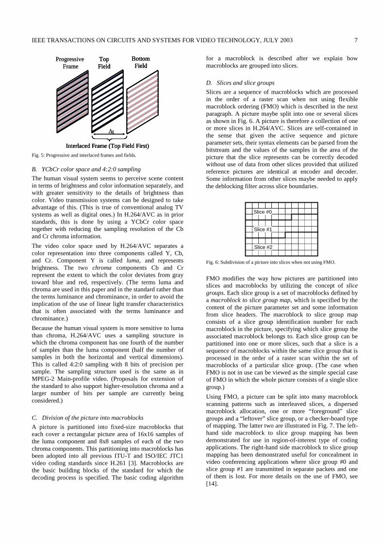
Generally, a frame of video can be considered to contain two interleaved fields, a top and a bottom field. The top field contains even-numbered rows 0, 2,..., H/2-1 with H being the number of rows of the frame. The bottom field contains the odd-numbered rows (starting with the second line of the frame). If the two fields of a frame were captured at different time instants, the frame is referred to as an interlaced frame, and otherwise it is referred to as a progressive frame (see Fig. 5). The coding representation in H.264/AVC is primarily agnostic with respect to this video characteristic, i.e., the underlying interlaced or progressive timing of the original captured pictures. Instead, its coding specifies a representation based primarily on geometric concepts rather than being based on timing.


ProgressiveFrame

TopField

BottomField

Interlaced Frame (Top Field First)

∆t

ProgressiveFrame

TopField

BottomField


TopField

BottomField


∆t

Fig. 5: Progressive and interlaced frames and fields.

B. YCbCr color space and 4:2:0 sampling

The human visual system seems to perceive scene content in terms of brightness and color information separately, and with greater sensitivity to the details of brightness than color. Video transmission systems can be designed to take advantage of this. (This is true of conventional analog TV systems as well as digital ones.) In H.264/AVC as in prior standards, this is done by using a YCbCr color space together with reducing the sampling resolution of the Cb and Cr chroma information.

The video color space used by H.264/AVC separates a color representation into three components called Y, Cb, and Cr. Component Y is called luma, and represents brightness. The two chroma components Cb and Cr represent the extent to which the color deviates from gray toward blue and red, respectively. (The terms luma and chroma are used in this paper and in the standard rather than the terms luminance and chrominance, in order to avoid the implication of the use of linear light transfer characteristics that is often associated with the terms luminance and chrominance.)

Because the human visual system is more sensitive to luma than chroma, H.264/AVC uses a sampling structure in which the chroma component has one fourth of the number of samples than the luma component (half the number of samples in both the horizontal and vertical dimensions). This is called 4:2:0 sampling with 8 bits of precision per sample. The sampling structure used is the same as in MPEG-2 Main-profile video. (Proposals for extension of the standard to also support higher-resolution chroma and a larger number of bits per sample are currently being considered.)

C. Division of the picture into macroblocks

A picture is partitioned into fixed-size macroblocks that each cover a rectangular picture area of 16x16 samples of the luma component and 8x8 samples of each of the two chroma components. This partitioning into macroblocks has been adopted into all previous ITU-T and ISO/IEC JTC1 video coding standards since H.261 [3]. Macroblocks are the basic building blocks of the standard for which the decoding process is specified. The basic coding algorithm

for a macroblock is described after we explain how macroblocks are grouped into slices.

D. Slices and slice groups

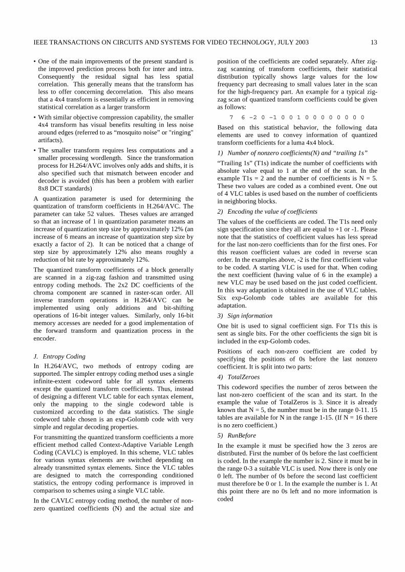
Slices are a sequence of macroblocks which are processed in the order of a raster scan when not using flexible macroblock ordering (FMO) which is described in the next paragraph. A picture maybe split into one or several slices as shown in Fig. 6. A picture is therefore a collection of one or more slices in H.264/AVC. Slices are self-contained in the sense that given the active sequence and picture parameter sets, their syntax elements can be parsed from the bitstream and the values of the samples in the area of the picture that the slice represents can be correctly decoded without use of data from other slices provided that utilized reference pictures are identical at encoder and decoder. Some information from other slices maybe needed to apply the deblocking filter across slice boundaries.

Slice #0

Slice #1

Slice #2

Slice #0

Slice #1

Slice #2

Fig. 6: Subdivision of a picture into slices when not using FMO.

FMO modifies the way how pictures are partitioned into slices and macroblocks by utilizing the concept of slice groups. Each slice group is a set of macroblocks defined by a macroblock to slice group map, which is specified by the content of the picture parameter set and some information from slice headers. The macroblock to slice group map consists of a slice group identification number for each macroblock in the picture, specifying which slice group the associated macroblock belongs to. Each slice group can be partitioned into one or more slices, such that a slice is a sequence of macroblocks within the same slice group that is processed in the order of a raster scan within the set of macroblocks of a particular slice group. (The case when FMO is not in use can be viewed as the simple special case of FMO in which the whole picture consists of a single slice group.)

Using FMO, a picture can be split into many macroblock scanning patterns such as interleaved slices, a dispersed macroblock allocation, one or more “foreground” slice groups and a “leftover” slice group, or a checker-board type of mapping. The latter two are illustrated in Fig. 7. The left-hand side macroblock to slice group mapping has been demonstrated for use in region-of-interest type of coding applications. The right-hand side macroblock to slice group mapping has been demonstrated useful for concealment in video conferencing applications where slice group #0 and slice group #1 are transmitted in separate packets and one of them is lost. For more details on the use of FMO, see [14].


Slice Group #0

Slice Group #1

Slice Group #2

Slice Group #0

Slice Group #1

Slice Group #2

Slice Group #0

Slice Group #1

Slice Group #2

Slice Group #0

Slice Group #1

Slice Group #0

Slice Group #1

Fig. 7: Subdivision of a QCIF frame into slices when utilizing FMO.

Regardless of whether FMO is in use or not, each slice can be coded using different coding types as follows:

• I slice: A slice in which all macroblocks of the slice are coded using intra prediction.

• P slice: In addition to the coding types of the I slice, some macroblocks of the P slice can also be coded using inter prediction with at most one motion-compensated prediction signal per prediction block.

• B slice: In addition to the coding types available in a P slice, some macroblocks of the B slice can also be coded using inter prediction with two motion-compensated prediction signals per prediction block.

The above three coding types are very similar to those in previous standards with the exception of the use of reference pictures as described below. The following two coding types for slices are new:

• SP slice: A so-called switching P slice that is coded such that efficient switching between different pre-coded pictures becomes possible.

• SI slice: A so-called switching I slice that allows an exact match of a macroblock in an SP slice for random access and error recovery purposes.

For details on the novel concept of SP and SI slices, the reader is referred to [15] while the other slice types are further described below.

E. Encoding and decoding process for macroblocks

All luma and chroma samples of a macroblock are either spatially or temporally predicted, and the resulting prediction residual is encoded using transform coding. For transform coding purposes, each color component of the prediction residual signal is subdivided into smaller 4x4 blocks. Each block is transformed using an integer transform, and the transform coefficients are quantized and encoded using entropy coding methods.

Fig. 8 shows a block diagram of the video coding layer for a macroblock. The input video signal is split into macroblocks, the association of macroblocks to slice groups and slices is selected, and then each macroblock of each slice is processed as shown. An efficient parallel processing of macroblocks is possible when there are various slices in the picture.

EntropyCoding

Scaling & Inv. Transform

Motion -Compensation

ControlData

Quant.Transf . coeffs

MotionData

Intra/Inter

CoderControl

Decoder

MotionEstimation

Transform/Scal ./Quant .-

InputVideoSignal

Split intoMacroblocks16x16 pixels

Intra -frame Prediction

DeblockingFilter

OutputVideoSignal

EntropyCoding



ControlData


MotionData

Intra/Inter

CoderControl

Decoder

MotionEstimation


InputVideoSignal



DeblockingFilter

OutputVideoSignal

EntropyCoding



ControlData


MotionData

Intra/Inter

CoderControl

Decoder

MotionEstimation


InputVideoSignal



DeblockingFilter

OutputVideoSignal

EntropyCoding



ControlData


MotionData

Intra/Inter

CoderControl

Decoder

MotionEstimation


InputVideoSignal



DeblockingFilter

OutputVideoSignal

Fig. 8: Basic coding structure for H.264/AVC for a macroblock.

F. Adaptive frame/field coding operation

In interlaced frames with regions of moving objects or camera motion, two adjacent rows tend to show a reduced degree of statistical dependency when compared to progressive frames in. In this case, it may be more efficient to compress each field separately. To provide high coding efficiency, the H.264/AVC design allows encoders to make any of the following decisions when coding a frame:

1. To combine the two fields together and to code them as one single coded frame (frame mode).

2. To not combine the two fields and to code them as separate coded fields (field mode).

3. To combine the two fields together and compress them as a single frame, but when coding the frame to split the pairs of two vertically adjacent macroblocks into either pairs of two field or frame macroblocks before coding them.

The choice between the three options can be made adaptively for each frame in a sequence. The choice between the first two options is referred to as picture-adaptive frame/field (PAFF) coding. When a frame is coded as two fields, each field is partitioned into macroblocks and is coded in a manner very similar to a frame, with the following main exceptions:

i. motion compensation utilizes reference fields rather than reference frames,

ii. the zig-zag scan of transform coefficients is different, and

iii. the strong deblocking strength is not used for filtering horizontal edges of macroblocks in fields, because the field rows are spatially twice as far apart as frame rows and the length of the filter thus covers a larger spatial area.

During the development of the H.264/AVC standard, PAFF coding was reported to reduce bit rates in the range of 16 to 20 % over frame-only coding mode for ITU-R 601 resolution sequences like "Canoa", "Rugby", etc.

If a frame consists of mixed regions where some regions are moving and others are not, it is typically more efficient to code the non-moving regions in frame mode and the moving regions in the field mode. Therefore, the frame/field encoding decision can also be made


independently for each vertical pair of macroblocks (a 16x32 luma region) in a frame. This coding option is referred to as macroblock-adaptive frame/field (MBAFF) coding. For a macroblock pair that is coded in frame mode, each macroblock contains frame lines. For a macroblock pair that is coded in field mode, the top macroblock contains top field lines and the bottom macroblock contains bottom field lines. Fig. 9 illustrates the MBAFF macroblock pair concept.

A Pair of Macroblocks in Frame Mode

Top/Bottom Macroblocks in Field Mode

A Pair of Macroblocks in Frame Mode

Top/Bottom Macroblocks in Field Mode

Fig. 9: Conversion of a frame macroblock pair into a field macroblock pair.

Note that, unlike in MPEG-2, the frame/field decision is made at the macroblock pair level rather than within the macroblock level. The reasons for this choice are to keep the basic macroblock processing structure intact, and to permit motion compensation areas as large as the size of a macroblock.

Each macroblock of a field macroblock pair is processed very similarly to a macroblock within a field in PAFF coding. However, since a mixture of field and frame macroblock pairs may occur within an MBAFF frame, the methods that are used for

1) zig-zag scanning

2) prediction of motion vectors

3) prediction of intra prediction modes

4) intra frame sample prediction

5) deblocking filtering

6) context modelling in entropy coding

are modified to account for this mixture. The main idea is to preserve as much spatial consistency as possible. It should be noted that the specification of spatial neighbours in MBAFF frames is rather complicated (please refer to [1]) and that in the next sections spatial neighbours are only described for non-MBAFF frames.

Another important distinction between MBAFF and PAFF is that in MBAFF, one field cannot use the macroblocks in the other field of the same frame as a reference for motion prediction (because some regions of each field are not yet available when a field macroblock of the other field is coded). Thus, sometimes PAFF coding can be more efficient than MBAFF coding (particularly in the case of

rapid global motion, scene change, or intra picture refresh), although the reverse is usually true.

During the development of the standard, MBAFF was reported to reduce bit rates in the range of 14 to 16% over PAFF for ITU-R 601 resolution sequences like "Mobile and Calendar" and "MPEG-4 World News".

G. Intra-frame Prediction

Each macroblock can be transmitted in one of several coding types depending on the slice-coding type. In all slice-coding types, the following types of intra coding are supported, which are denoted as Intra_4x4 or Intra_16x16 together with chroma prediction and I_PCM prediction modes.

The Intra_4x4 mode is based on predicting each 4x4 luma block separately and is well suited for coding of parts of a picture with significant detail. The Intra_16x16 mode, on the other hand, does prediction of the whole 16x16 luma block and is more suited for coding very smooth areas of a picture. In addition to these two types of luma prediction, a separate chroma prediction is conducted. As an alternative to Intra_4x4 and Intra_16x16, the I_PCM coding type allows the encoder to simply bypass the prediction and transform coding processes and instead directly send the values of the encoded samples. The I_PCM mode serves the following purposes:

1) It allows the encoder to precisely represent the values of the samples

2) It provides a way to accurately represent the values of anomalous picture content without significant data expansion

3) It enables placing a hard limit on the number of bits a decoder must handle for a macroblock without harm to coding efficiency.

In contrast to some previous video coding standards (namely H.263+ and MPEG-4 Visual), where intra prediction has been conducted in the transform domain intra prediction in H.264/AVC is always conducted in the spatial domain, by referring to neighboring samples of previously-coded blocks which are to the left and/or above the block to be predicted. This may incur error propagation in environments with transmission errors that propagate due to motion compensation into inter-coded macroblocks. Therefore, a constrained intra coding mode can be signaled that allows prediction only from intra-coded neighboring macroblocks.

When using the Intra_4x4 mode, each 4x4 block is predicted from spatially neighboring samples as illustrated on the left-hand side of Fig. 10. The 16 samples of the 4x4 block which are labeled as a-p are predicted using prior decoded samples in adjacent blocks labeled as A-Q. For each 4x4 block one of nine prediction modes can be utilized. In addition to "DC" prediction (where one value is used to predict the entire 4x4 block), eight directional prediction modes are specified as illustrated on the right-hand side of Fig. 10. Those modes are suitable to predict


directional structures in a picture such as edges at various angles.

Q A B C D E F G HI a b c dJ e f g hK i j k lL m n o p

Q A B C D E F G HI a b c dJ e f g hK i j k lL m n o p 0

1

43

57

8

6

Fig. 10: Left: Intra_4x4 prediction is conducted for samples a-p of a block using samples A-Q. Right: 8 "prediction directions" for Intra_4x4 prediction.

Fig. 11 shows five of the nine Intra_4x4 prediction modes. For mode 0 (vertical prediction) the samples above the 4x4 block are copied into the block as indicated by the arrows. Mode 1 (horizontal prediction) operates in a manner similar to vertical prediction except that the samples to the left of the 4x4 block are copied. For mode 2 (DC prediction) the adjacent samples are averaged as indicated in Fig. 11. The remaining 6 modes are diagonal prediction modes which are called diagonal-down-left, diagonal-down-right, vertical-right, horizontal-down, vertical-left, and horizontal-up prediction. As their names indicate, they are suited to predict textures with structures in the specified direction. The first two diagonal prediction modes are also illustrated in Fig. 11. When samples E-H (ref. to Fig. 10) that are used for the diagonal-down-left prediction mode are not available (because they have not yet been decoded or they are outside of the slice or not in an intra-coded macroblock in the constrained intra-mode) these samples are replaced by sample D. Note that in earlier draft versions of the Intra_4x4 prediction mode the four samples below sample L were also used for some prediction modes. However, due to the need to reduce memory access, these have been dropped, as the relative gain for their use is very small.

Mode 0 - VerticalMode 0 - Vertical

Mode 1 - HorizontalMode 1 - Horizontal

Mode 2 - DC

+

++

+ + ++

Mode 2 - DC

+

++

+ + ++

Mode 3 – Diagonal Down/LeftMode 3 – Diagonal Down/Left Mode 4 – Diagonal Down/RightMode 4 – Diagonal Down/Right

Fig. 11: Five of the nine Intra_4x4 prediction modes.

When utilizing the Intra_16x16 mode, the whole luma component of a macroblock is predicted. Four prediction modes are supported. Prediction mode 0 (vertical prediction), mode 1 (horizontal prediction), and mode 2 (DC prediction) are specified similar to the modes in Intra_4x4 prediction except that instead of 4 neighbors on

each side to predict a 4x4 block, 16 neighbors on each side to predict a 16x16 block are used. For the specification of prediction mode 4 (plane prediction) please refer to [1].

The chroma samples of a macroblock are predicted using a similar prediction technique as for the luma component in Intra_16x16 macroblocks, since chroma is usually smooth over large areas.

Intra prediction (and all other forms of prediction) across slice boundaries is not used, in order to keep all slices independent of each other.

H. Inter-frame Prediction

1) Inter-frame Prediction in P Slices

In addition to the intra macroblock coding types, various predictive or motion-compensated coding types are specified as P macroblock types. Each P macroblock type corresponds to a specific partition of the macroblock into the block shapes used for motion-compensated prediction. Partitions with luma block sizes of 16x16, 16x8, 8x16, and 8x8 samples are supported by the syntax. In case partitions with 8x8 samples are chosen, one additional syntax element for each 8x8 partition is transmitted. This syntax element specifies whether the corresponding 8x8 partition is further partitioned into partitions of 8x4, 4x8, or 4x4 luma samples and corresponding chroma samples. Fig. 12 illustrates the partitioning.

8x8

0

4x8

0 1 0 1

2 3

4x4 8x4

1

0 8x8 Types

0

16x16

0 1

8x16 M

Types

8x8 0 1

2 3

16x8

1

0

Fig. 12: Segmentations of the macroblock for motion compensation. Top: segmentation of macroblocks, bottom: segmentation of 8x8 partitions.

The prediction signal for each predictive-coded MxN luma block is obtained by displacing an area of the corresponding reference picture, which is specified by a translational motion vector and a picture reference index. Thus, if the macroblock is coded using four 8x8 partitions and each 8x8 partition is further split into four 4x4 partitions, a maximum of sixteen motion vectors may be transmitted for a single P macroblock.

The accuracy of motion compensation is in units of one quarter of the distance between luma samples. In case the motion vector points to an integer-sample position, the prediction signal consists of the corresponding samples of the reference picture; otherwise the corresponding sample is obtained using interpolation to generate non-integer positions. The prediction values at half-sample positions are obtained by applying a one-dimensional 6-tap FIR filter horizontally and vertically. Prediction values at quarter-sample positions are generated by averaging samples at integer- and half-sample positions.


Fig. 13 illustrates the fractional sample interpolation for samples a-k and n-r. The samples at half sample positions labeled b and h are derived by first calculating intermediate values b1 and h1, respectively by applying the 6-tap filter as follows:

b1 = ( E – 5 F + 20 G + 20 H – 5 I + J )

h1 = ( A – 5 C + 20 G + 20 M – 5 R + T )

The final prediction values for locations b and h are obtained as follows and clipped to the range of 0 to 255.

b = ( b1 + 16 ) >> 5

h = ( h1 + 16 ) >> 5

The samples at half sample positions labeled as j are obtained by

j1 = cc – 5 dd + 20 h1 + 20 m1 – 5 ee + ff,

where intermediate values denoted as cc, dd, ee, m1 and ff are obtained in a manner similar to h1. The final prediction value j is then computed as j = ( j1 + 512 ) >> 10 and is clipped to the range of 0 to 255. The two alternative methods of obtaining the value of j illustrate that the filtering operation is truly separable for the generation of the half-sample positions.

The samples at quarter sample positions labeled as a, c, d, n, f, i, k, and q are derived by averaging with upward rounding of the two nearest samples at integer and half sample positions as, for example, by

a = ( G + b + 1 ) >> 1.

The samples at quarter sample positions labelled as e, g, p, and r are derived by averaging with upward rounding of the two nearest samples at half sample positions in the diagonal direction as, for example, by

e = ( b + h + 1 ) >> 1.

bb

a cE F I JG

h

d

n

H

m

A

C

B

D

R

T

S

U

M s NK L P Q

fe g

ji k

qp r

aa

b

cc dd ee ff

hh

gg

Fig. 13: Filtering for fractional-sample accurate motion compensation. Upper-case letters indicate samples on the full-sample grid, while lower case samples indicate samples in between at fractional-sample positions.

The prediction values for the chroma component are always obtained by bi-linear interpolation. Since the sampling grid of chroma has lower resolution than the sampling grid of

the luma, the displacements used for chroma have one-eighth sample position accuracy.

The more accurate motion prediction using full sample, half sample and one-quarter sample prediction represent one of the major improvements of the present method compared to earlier standards for the following two reasons:

• The most obvious reason is more accurate motion representation

• The other reason is more flexibility in prediction filtering. Full sample, half sample and one-quarter sample prediction represent different degrees of low pass filtering which is chosen automatically in the motion estimation process. In this respect the 6-tap filter turns out to be a much better trade-off between necessary prediction loop filtering and has the ability to preserve high frequency content in the prediction loop.

A more detailed investigation of fractional sample accuracy is presented in [8].

The syntax allows so-called motion vectors over picture boundaries, i.e. motion vectors that point outside the image area. In this case, the reference frame is extrapolated beyond the image boundaries by repeating the edge samples before interpolation.

The motion vector components are differentially coded using either median or directional prediction from neighbouring blocks. No motion vector component prediction (or any other form of prediction) takes place across slice boundaries.

The syntax supports multi-picture motion-compensated prediction [9][10]. That is, more than one prior coded picture can be used as reference for motion-compensated prediction. Figure 3 illustrates the concept.

CurrentPicture

4 Prior Decoded Picturesas Reference

∆ = 2∆ = 4

∆ = 1

CurrentPicture

4 Prior Decoded Picturesas Reference

∆ = 2∆ = 4

∆ = 1

Fig. 14: Multi-frame motion compensation. In addition to the motion vector, also picture reference parameters (∆) are transmitted. The concept is also extended to B slices as described below.

Multi-frame motion-compensated prediction requires both encoder and decoder to store the reference pictures used for inter prediction in a multi-picture buffer. The decoder replicates the multi-picture buffer of the encoder according to memory management control operations specified in the bitstream. Unless the size of the multi-picture buffer is set to one picture, the index at which the reference picture is located inside the multi-picture buffer has to be signalled. The reference index parameter is transmitted for each


motion-compensated 16x16, 16x8, 8x16, or 8x8 luma block. Motion compensation for smaller regions than 8x8 use the same reference index for prediction of all blocks within the 8x8 region.

In addition to the motion-compensated macroblock modes described above, a P macroblock can also be coded in the so-called P_Skip type. For this coding type, neither a quantized prediction error signal, nor a motion vector or reference index parameter is transmitted. The reconstructed signal is obtained similar to the prediction signal of a P_16x16 macroblock type that references the picture which is located at index 0 in the multi-picture buffer. The motion vector used for reconstructing the P_Skip macroblock is similar to the motion vector predictor for the 16x16 block. The useful effect of this definition of the P_Skip coding type is that large areas with no change or constant motion like slow panning can be represented with very few bits.

2) Inter-frame Prediction in B Slices

In comparison to prior video coding standards, the concept of B slices is generalized in H.264/AVC. This extension refers back to [11] and is further investigated in [12]. For example, other pictures can reference pictures containing B slices for motion-compensated prediction, depending on the memory management control operation of the multi-picture buffering. Thus, the substantial difference between B and P slices is that B slices are coded in a manner in which some macroblocks or blocks may use a weighted average of two distinct motion-compensated prediction values for building the prediction signal. B slices utilize two distinct lists of reference pictures, which are referred to as the first (list 0) and second (list 1) reference picture lists, respectively. Which pictures are actually located in each reference picture list is an issue of the multi-picture buffer control and an operation very similar to the conventional MPEG-2 B pictures can be enabled if desired by the encoder.

In B slices, four different types of inter-picture prediction are supported: list 0, list 1, bi-predictive, and direct prediction. For the bi-predictive mode, the prediction signal is formed by a weighted average of motion-compensated list 0 and list 1 prediction signals. The direct prediction mode is inferred from previously transmitted syntax elements and can be either list 0 or list 1 prediction or bi-predictive.

B slices utilize a similar macroblock partitioning as P slices. Beside the P_16x16, P_16x8, P_8x16, P_8x8, and the intra coding types, bi-predictive prediction and another type of prediction called direct prediction, are provided. For each 16x16, 16x8, 8x16, and 8x8 partition, the prediction method (list 0, list 1, bi-predictive) can be chosen separately. An 8x8 partition of a B macroblock can also be coded in direct mode. If no prediction error signal is transmitted for a direct macroblock mode, it is also referred to as B_Skip mode and can be coded very efficiently similar to the P_Skip mode in P slices. The motion vector coding is similar to that of P slices with the appropriate modifications because neighbouring blocks may be coded using different prediction modes.

I. Transform, Scaling, and Quantization

Similar to previous video coding standards, H.264/AVC utilizes transform coding of the prediction residual. However, in H.264/AVC, the transformation is applied to 4x4 blocks, and instead of a 4x4 discrete cosine transform (DCT), a separable integer transform with similar properties as a 4x4 DCT is used. The transform matrix is given as

−−−−

−−=

1221

1111

2112

1111

H

Since the inverse transform is defined by exact integer operations, inverse-transform mismatches are avoided. The basic transform coding process is very similar to that of previous standards. At the encoder the process includes a forward transform, zig-zag scanning, scaling and rounding as the quantization process followed by entropy coding. At the decoder, the inverse of the encoding process is performed except for the rounding. More details on the specific aspects of the transform in H.264/AVC can be found in [17].

It has already been mentioned that Intra_16x16 prediction modes and chroma intra modes are intended for coding of smooth areas. For that reason the DC coefficients undergo a second transform with the result that we have transform coefficients covering the whole macroblock. An additional 2x2 transform is also applied to the DC coefficients of the four 4x4 blocks of each chroma component. The procedure for a chroma block is illustrated in Fig. 15. The small blocks inside the larger blocks represent DC coefficients of each of the four 4x4 chroma blocks of a chroma component of a macroblock numbered as 0,1,2, and 3. The two indices correspond to the indices of the 2x2 inverse Hadamard transform.

To explain the idea behind these repeated transforms, let us point to a general property of a two-dimensional transform of very smooth content (where sample correlation approaches 1). In that situation the reconstruction accuracy is proportional to the inverse of the one dimensional size of the transform. Hence, for a very smooth area, the reconstruction error with a transform covering the complete 8x8 block is halved compared to using only 4x4 transform. A similar rationale can be used for the second transform connected to the INTRA-16x16 mode.

0 1

2 3

00 01

10 11

Fig. 15: Repeated transform for chroma blocks. The four blocks numbered 0 to 3 indicate the four chroma blocks of a chroma component of a macroblock.

There are several reasons for using a smaller size transform:


• One of the main improvements of the present standard is the improved prediction process both for inter and intra. Consequently the residual signal has less spatial correlation. This generally means that the transform has less to offer concerning decorrelation. This also means that a 4x4 transform is essentially as efficient in removing statistical correlation as a larger transform

• With similar objective compression capability, the smaller 4x4 transform has visual benefits resulting in less noise around edges (referred to as “mosquito noise” or "ringing" artifacts).

• The smaller transform requires less computations and a smaller processing wordlength. Since the transformation process for H.264/AVC involves only adds and shifts, it is also specified such that mismatch between encoder and decoder is avoided (this has been a problem with earlier 8x8 DCT standards)

A quantization parameter is used for determining the quantization of transform coefficients in H.264/AVC. The parameter can take 52 values. Theses values are arranged so that an increase of 1 in quantization parameter means an increase of quantization step size by approximately 12% (an increase of 6 means an increase of quantization step size by exactly a factor of 2). It can be noticed that a change of step size by approximately 12% also means roughly a reduction of bit rate by approximately 12%.

The quantized transform coefficients of a block generally are scanned in a zig-zag fashion and transmitted using entropy coding methods. The 2x2 DC coefficients of the chroma component are scanned in raster-scan order. All inverse transform operations in H.264/AVC can be implemented using only additions and bit-shifting operations of 16-bit integer values. Similarly, only 16-bit memory accesses are needed for a good implementation of the forward transform and quantization process in the encoder.

J. Entropy Coding

In H.264/AVC, two methods of entropy coding are supported. The simpler entropy coding method uses a single infinite-extent codeword table for all syntax elements except the quantized transform coefficients. Thus, instead of designing a different VLC table for each syntax element, only the mapping to the single codeword table is customized according to the data statistics. The single codeword table chosen is an exp-Golomb code with very simple and regular decoding properties.

For transmitting the quantized transform coefficients a more efficient method called Context-Adaptive Variable Length Coding (CAVLC) is employed. In this scheme, VLC tables for various syntax elements are switched depending on already transmitted syntax elements. Since the VLC tables are designed to match the corresponding conditioned statistics, the entropy coding performance is improved in comparison to schemes using a single VLC table.

In the CAVLC entropy coding method, the number of non-zero quantized coefficients (N) and the actual size and

position of the coefficients are coded separately. After zig-zag scanning of transform coefficients, their statistical distribution typically shows large values for the low frequency part decreasing to small values later in the scan for the high-frequency part. An example for a typical zig-zag scan of quantized transform coefficients could be given as follows:

7 6 –2 0 –1 0 0 1 0 0 0 0 0 0 0 0

Based on this statistical behavior, the following data elements are used to convey information of quantized transform coefficients for a luma 4x4 block.

1) Number of nonzero coefficients(N) and “trailing 1s”

“Trailing 1s” (T1s) indicate the number of coefficients with absolute value equal to 1 at the end of the scan. In the example T1s = 2 and the number of coefficients is N = 5. These two values are coded as a combined event. One out of 4 VLC tables is used based on the number of coefficients in neighboring blocks.

2) Encoding the value of coefficients

The values of the coefficients are coded. The T1s need only sign specification since they all are equal to +1 or -1. Please note that the statistics of coefficient values has less spread for the last non-zero coefficients than for the first ones. For this reason coefficient values are coded in reverse scan order. In the examples above, -2 is the first coefficient value to be coded. A starting VLC is used for that. When coding the next coefficient (having value of 6 in the example) a new VLC may be used based on the just coded coefficient. In this way adaptation is obtained in the use of VLC tables. Six exp-Golomb code tables are available for this adaptation.

3) Sign information

One bit is used to signal coefficient sign. For T1s this is sent as single bits. For the other coefficients the sign bit is included in the exp-Golomb codes.

Positions of each non-zero coefficient are coded by specifying the positions of 0s before the last nonzero coefficient. It is split into two parts:

4) TotalZeroes

This codeword specifies the number of zeros between the last non-zero coefficient of the scan and its start. In the example the value of TotalZeros is 3. Since it is already known that N = 5, the number must be in the range 0-11. 15 tables are available for N in the range 1-15. (If N = 16 there is no zero coefficient.)

5) RunBefore

In the example it must be specified how the 3 zeros are distributed. First the number of 0s before the last coefficient is coded. In the example the number is 2. Since it must be in the range 0-3 a suitable VLC is used. Now there is only one 0 left. The number of 0s before the second last coefficient must therefore be 0 or 1. In the example the number is 1. At this point there are no 0s left and no more information is coded


The efficiency of entropy coding can be improved further if the Context-Adaptive Binary Arithmetic Coding (CABAC) is used [16]. On the one hand, the usage of arithmetic coding allows the assignment of a non-integer number of bits to each symbol of an alphabet, which is extremely beneficial for symbol probabilities that are greater than 0.5. On the other hand, the usage of adaptive codes permits adaptation to non-stationary symbol statistics. Another important property of CABAC is its context modelling. The statistics of already coded syntax elements are used to estimate conditional probabilities. These conditional probabilities are used for switching several estimated probability models. In H.264/AVC, the arithmetic coding core engine and its associated probability estimation are specified as multiplication-free low-complexity methods using only shifts and table look-ups. Compared to CAVLC, CABAC typically provides a reduction in bit rate between 5-15% The highest gains are typically obtained when coding interlaced TV signals. More details on CABAC can be found in [16].

K. In-Loop Deblocking Filter

One particular characteristic of block-based coding is the accidental production of visible block structures. Block edges are typically reconstructed with less accuracy than interior pixels and “blocking” is generally considered to be one of the most visible artifacts with the present compression methods. For this reason, H.264/AVC defines an adaptive in-loop deblocking filter, where the strength of filtering is controlled by the values of several syntax elements. A detailed description of the adaptive deblocking filter can be found in [18].

Fig. 16 illustrates the principle of the deblocking filter using a visualization of a one-dimensional edge. Whether the samples p0 and q0 as well as p1 and q1 are filtered is determined using quantization parameter (QP) dependent thresholds α(QP) and β(QP). Thus, filtering of p0 and q0 only takes place if each of the following conditions is satisfied:

1. | p0 - q0 | < α(QP)

2. | p1 - p0 | < β(QP)

3. | q1 - q0 | < β(QP)

where the β(QP) is considerably smaller than α(QP). Accordingly, filtering of p1 or q1 takes place if the corresponding condition below is satisfied:

| p2 - p0 | < β(QP) or | q2 - q0 | < β(QP)

The basic idea is that if a relatively large absolute difference between samples near a block edge is measured, it is quite likely a blocking artifact and should therefore be reduced. However, if the magnitude of that difference is so large that it cannot be explained by the coarseness of the quantization used in the encoding, the edge is more likely to reflect the actual behavior of the source picture and should not be smoothed over.

4x4 Block Edge

p0

q0

p1

p2

q 1q 2

4x4 Block Edge 4x4 Block Edge

p0

q0

p1

p2

q 1q 2

4x4 Block Edge Fig. 16: Principle of Deblocking Filter.

The blockiness is reduced, while the sharpness of the content is basically unchanged. Consequently, the subjective quality is significantly improved. The filter reduces bit rate typically by 5-10% while producing the same objective quality as the non-filtered video. Fig. 17 illustrates the performance of the deblocking filter.

Fig. 17: Performance of the deblocking filter for highly compressed pictures. Left: without deblocking filter, right: with deblocking filter.

L. Hypothetical Reference Decoder

One of the key benefits provided by a standard is the assurance that all the decoders compliant with the standard will be able to decode a compliant compressed video. To achieve that it is not sufficient to just provide a description of the coding algorithm. It is also important in a real time system to specify how bits are fed to a decoder and how the decoded pictures are removed from a decoder. Specifying input and output buffer models and developing an implementation independent model of a receiver achieves this. That receiver model is also called Hypothetical Reference Decoder (HRD) and is described in detail in [19]. An encoder is not allowed to create a bitstream that cannot be decoded by the HRD. Hence, if in any receiver implementation the designer mimics the behaviour of HRD, it is guaranteed to be able to decode all the compliant bitstreams.

In H.264/AVC HRD specifies operation of two buffers: (i) Coded Picture Buffer (CPB) and (ii) Decoded Picture Buffer (DPB). CPB models the arrival and removal time of the coded bits. The HRD design is similar in spirit to what MPEG-2 had, but is more flexible in support of sending the video at a variety of bit rates without excessive delay.

As unlike MPEG-2, in H.264/AVC, multiple frames can be used for reference, the reference frames can be located either in past or future arbitrarily in display order, the HRD


also specifies a model of the decoded picture buffer management to ensure that excessive memory capacity is not needed in a decoder to store the pictures used as references.

V. PROFILES & POTENTIAL APPLICATIONS

A. Profiles and levels

Profiles and levels specify conformance points. These conformance points are designed to facilitate interoperability between various applications of the standard that have similar functional requirements. A profile defines a set of coding tools or algorithms that can be used in generating a conforming bit-stream, whereas a level places constraints on certain key parameters of the bitstream.

All decoders conforming to a specific profile must support all features in that profile. Encoders are not required to make use of any particular set of features supported in a profile but have to provide conforming bitstreams, i.e. bitstreams that can be decoded by conforming decoders. In H.264/AVC, three profiles are defined, which are the Baseline, Main, and Extended Profile.

The Baseline profile supports all features in H.264/AVC except the following two feature sets:

- Set 1: B slices, weighted prediction, CABAC, field coding, and picture or macroblock adaptive switching between frame and field coding.

- Set 2: SP/SI slices, and slice data partitioning.

The first set of additional features is supported by the Main profile. However, the Main profile does not support the FMO, ASO, and redundant pictures features which are supported by the Baseline profile. Thus, only a subset of the coded video sequences that are decodable by a Baseline profile decoder can be decoded by a Main profile decoder. (Flags are used in the sequence parameter set to indicate which profiles of decoder can decode the coded video sequence.)

The Extended Profile supports all features of the Baseline profile, and both sets of features on top of Baseline profile, except for CABAC.

In H.264/AVC, the same set of level definitions is used with all profiles, but individual implementations may support a different level for each supported profile. Fifteen levels are defined specifying upper limits for the picture size (in macroblocks) ranging from QCIF to all the way to above 4k x 2k, decoder-processing rate (in macroblocks per second) ranging from 250k pixels per sec to 250M pixels per sec, size of the multi-picture buffers, video bit rate ranging from 64 kbps to 240 Mbps, and video buffer size.

B. Areas for the profiles of the new standard to be used

The increased compression efficiency of H.264/AVC offers to enhance existing applications or enables new

applications. A list of possible application areas is provided below.

• Conversational services which operate typically below 1 Mbps with low latency requirements. The ITU-T SG16 is currently modifying its systems recommendations to support H.264/AVC use in such applications, and the IETF is working on design of an RTP payload packetization. In the near term, these services would probably utilize the Baseline profile (possibly progressing over time to also use other profiles such as the Extended profile). Some specific applications in this category are given below.

- H.320 conversational video services that utilize circuit-switched ISDN-based video conferencing.

- 3GPP conversational H.324/M services.

- H.323 conversational services over the Internet with best effort IP/RTP protocols.

- 3GPP conversational services using IP/RTP for transport and SIP for session set-up.

• Entertainment video applications which operate between 1-8+ Mbps with moderate latency such as 0.5 to 2 seconds. The H.222.0 | MPEG-2 Systems specification is being modified to support these application. These applications would probably utilize the Main profile and include

- Broadcast via satellite, cable, terrestrial, or DSL

- DVD for standard and high-definition video

- Video on demand via various channels.

• Streaming services which typically operate at 50 kbps – 1.5 Mbps and have 2 or more seconds of latency. These services would probably utilize the Baseline or Extended profile and may be distinguished by whether they are used in wired or wireless environments as follows:

- 3GPP streaming using IP/RTP for transport and RTSP for session set-up. This extension of the 3GPP specification would likely use Baseline profile only.

- Streaming over the wired Internet using IP/RTP protocol and RTSP for session set-up. This domain which is currently dominated by powerful proprietary solutions might use the Extended profile and may require integration with some future system designs.

• Other Services that operate at lower bit rates and are distributed via file transfer and therefore do not impose delay constraints at all, which can potentially be served by any of the three profiles depending on various other systems requirements, are

- 3GPP multimedia messaging services

- Video mail


VI. HISTORY AND STANDARDIZATION PROCESS

In this section, we illustrate the history of the standard. The development of H.264/AVC is characterized by improvements in small steps over the last 3-4 years as can be seen from Fig. 18. In Fig. 18 the coding performance is shown for two example progressive-scan video sequences, when enabling the typical coding options for the various versions of the standard since August 1999 until completion in April 2003. The dates and creation of the various versions are shown in Tab. I. The document and the software versions have been called test model long-term (TML) when being developed in VCEG and joint model (JM) when the development was continued in the joint video team (JVT) as a partnership between MPEG and VCEG. The development took place in small steps between each version of the design as can be seen from Fig. 18.

TABLE I HISTORY OF H.264/AVC STANDARDIZATION PROCESS. FOR TML

VERSIONS WITH A *, NO SOFTWARE HAS BEEN CREATED. No TML/JM Date Location

1 TML-1 Aug. 1999 Berlin, Germany

2 TML-2* Oct. 1999 Red Bank, NJ, USA

3 TML-3 Feb. 2000 Geneva, Switzerland

4 TML-4 May, 2000 Osaka, Japan

5 TML-5 Aug. 2000 Portland, OR, USA

6 TML-6 Jan. 2001 Eibsee, Germany

7 TML-7* Apr. 2001 Austin, TX, USA

8 TML-8 May 2001 Porto Seguro, Brazil

9 TML-9 Sep. 2001 Santa Barbara, CA, USA

10 JM-1 Dec. 2001 Pattaya, Thailand

11 JM-2 Feb. 2002 Geneva, Switzerland

12 JM-3 May 2002 Fairfax, VA, USA

13 JM-4 July 2002 Klagenfurt, Austria

14 JM-5 Oct. 2002 Geneva, Switzerland

15 JM-6 Dec. 2002 Awaji, Japan

16 Final Mar. 2003 Pattaya, Thailand

The work started in VCEG as a parallel activity to the completion of the last version of H.263. The first Test Model Long-Term (TML-1, curve with circles in Fig. 18) was produced in August 1999. TML-1 was similar to H.263 by using a combination of block prediction and block transform/quantization/coding of the residual signal. The PSNR performance of TML-1 was similar to that of H.263 (curve with diamond-shaped markers in Fig. 18) and below MPEG-4 ASP (curve with star-shaped markers in Fig. 18). However, the starting point was considered sufficient due to some perceptual benefits being shown and a judgment that the design could be incrementally improved. The results shown for H.263 and MPEG-4 ASP have been optimized using Lagrangian methods as described in [13]. The main coding features of TML-1 are summarized as follows:

- 7 block partitions for inter prediction of a macroblock. The luminance component of a macroblock could be

partitioned into 16x16, 16x8, 8x16, 8x8, 8x4, 4x8 or 4x4 blocks in a similar way as depicted in Fig. 12. The 16x16, 16x8, 8x16, and 8x8 blocks have remained in the design. Partitioning into smaller blocks was modified later (in JM-2.1) into a tree-structured macroblock partition as described above.

- 1/3-sample accurate motion-compensated prediction using 4-tap filter in horizontal and vertical direction. The filter taps were (-1, 12, 6, –1)/16 and (-1, 6, 12, -1)/16. One of the sample positions used a stronger low pass filter for more flexible prediction loop filtering. This was modified later (in TML-4) to 1/4-sample accurate prediction using a 6-tap as described above. For TML-2 a method called adaptive motion accuracy (AMA) was adopted which has never been implemented into the software. AMA was dropped due to lack of coding efficiency improvement in TML-4. In TML-7/8, 1/8-sample accurate motion compensation was introduced which was then dropped for complexity reasons in JM-5.

- Multiple reference frames, the decoupling of temporal order and display order, and the decoupling of picture type from the ability to use pictures as references were envisioned from the beginning, but were integrated in the software and draft text rather gradually.

- Intra prediction was done on 4x4 blocks and based on the neighboring samples. There were 5 prediction modes which were the ones shown in Fig. 11 except with a simpler version of Mode 3. The number of prediction modes was increased to 7 in TML-4 and further increased to 9 in JM-2. In TML-3, the Intra_16x16 prediction mode was introduced and in JM-3, the various prediction modes for chroma have been introduced.

- The transform for the residual signal had size 4x4. This was in contrast to all previous standards which used transform size 8x8. The transform was also no longer exact DCT but an integer transform very close to DCT. The integer definition resulted in an exact definition of the inverse transform. The transform had basis vectors:

−−−−−

=

717177

13131313

177717

13131313

H

The transform was later changed to the version described above in JM-2.

- An in-loop deblocking filter similar to the one used in H.263 was in TML-1, but only on intra frames. This filter has been considerably refined during the entire development of the standard.

- Entropy coding used one single exp-Golomb type VLC table for all syntax elements (including transform coefficients). This was extended later by CABAC in TML-7 and CAVLC for transform coefficients in JM-3.

TML-1 did not contain many of the features of the final design of JM-6 (squares in Fig. 18) including interlace


support, B pictures and the network abstraction layer. The method of handling of interlaced video was among the last things integrated into the design (note that Fig. 18 does not

show performance for interlaced video). The improvement of JM-6 relative to TML-1 is typically between 2-3 dB PSNR or between 40-60 % in bit-rate reduction.

10 20 30 40 50 60 70 80 90 100 11026

28

30

32

34

36

38

Bit-rate [kbps]

PS

NR

[dB

]

TML-1 TML-3 TML-4 TML-5 TML-6 TML-8 TML-9 JM-1.9 JM-2.1 JM-3.4 JM-4.0d JM-5.0c JM-6.1e H.263+ MPEG-4 ASP

0 200 400 600 800 1000 1200 1400 1600 1800 200024

26

28

30

32

34

36

38

40

Bit-rate [kbps]

PS

NR

[dB

]

Fig. 18: Evolution of H.264/AVC since August 1999 until March 2003. Top: QCIF sequence Foreman coded at 10 Hz, bottom: CIF sequence Tempete coded at 30 Hz. The legend in the top figure indicates the various versions that have been run with typical settings.


I. CONCLUSIONS

The emerging H.264/AVC video coding standard has been developed and standardized collaboratively by both the ITU-T VCEG and ISO/IEC MPEG organizations. H.264/AVC represents a number of advances in standard video coding technology, in terms of both coding efficiency enhancement and flexibility for effective use over a broad variety of network types and application domains. Its video coding layer design is based on conventional block-based motion-compensated hybrid video coding concepts, but with some important differences relative to prior standards. We summarize some of the important differences thusly:

• Enhanced motion prediction capability

• Use of a small block-size exact-match transform

• Adaptive in-loop deblocking filter

• Enhanced entropy coding methods

When used well together, the features of the new design provide approximately a 50% bit rate savings for equivalent perceptual quality relative to the performance of prior standards (especially for higher-latency applications which allow some use of reverse temporal prediction).

Further information and documents of the project is available by ftp at ftp://ftp.imtc-files.org/jvt-experts.

II. ACKNOWLEDGEMENT

The authors thank the experts of ITU-T VCEG, ISO/IEC MPEG, and the ITU-T/ISO/IEC Joint Video Team for their contributions. Thanks to Karsten Sühring and Heiko Schwarz for providing the data for the comparison of the various TML and JM versions.

REFERENCES

[1] Joint Video Team of ITU-T and ISO/IEC JTC 1, “Draft ITU-T Recommendation and Final Draft International Standard of Joint Video Specification (ITU-T Rec. H.264 | ISO/IEC 14496-10 AVC),” Joint Video Team (JVT) of ISO/IEC MPEG and ITU-T VCEG, JVT-G050, March 2003.

[2] ITU-T and ISO/IEC JTC 1, “Generic coding of moving pictures and associated audio information – Part 2: Video,” ITU-T Recommendation H.262 – ISO/IEC 13818-2 (MPEG-2), Nov. 1994.

[3] ITU-T, Video Codec for Audiovisual Services at px64 kbit/s, ITU-T Recommendation H.261, Version 1: Nov. 1990; Version 2: Mar. 1993.

[4] ITU-T, “Video coding for low bit rate communication,” ITU-T Recommendation H.263; version 1, Nov. 1995; version 2, Jan. 1998; version 3, Nov. 2000.

Thomas Wiegand is with HHI.

Gary Sullivan is with Microsoft Corp.

Gisle Bjontegaard is with Tandberg.

Ajay Luthra is with Motorola Inc.

[5] ISO/IEC JTC1, “Coding of audio-visual objects – Part 2: Visual,” ISO/IEC 14496-2 (MPEG-4 visual version 1), April 1999; Amendment 1 (version 2), February, 2000; Amendment 4 (streaming profile), January, 2001.

[6] S. Wenger, "H.264/AVC over IP," in IEEE Transactions on Circuits and Systems for Video Technology, this issue.

[7] T. Stockhammer, M. M. Hannuksela, and T. Wiegand, "H.264/AVC in Wireless Environments," in IEEE Transactions on Circuits and Systems for Video Technology, this issue

[8] T. Wedi, "Motion Compensation in H.264/AVC," in IEEE Transactions on Circuits and Systems for Video Technology, this issue.

[9] T. Wiegand, X. Zhang, and B. Girod, “Long-Term Memory Motion-Compensated Prediction,” IEEE Transactions on Circuits and Systems for Video Technology, vol. 9, no. 1, pp. 70-84, Feb. 1999.

[10] T. Wiegand and B. Girod, “Multi-frame Motion-Compensated Prediction for Video Transmission,” Kluwer Academic Publishers, Sept. 2001.

[11] M. Flierl, T. Wiegand, and B. Girod, "A Locally Optimal Design Algorithm for Block-Based Multi-Hypothesis Motion-Compensated Prediction", in Data Compression Conference, Snowbird, USA, Mar. 1998, pp. 239-248.

[12] M. Flierl and B. Girod. “Generalized B Pictures and the Draft JVT/H.264 Video Compression Standard”, in IEEE Transactions on Circuits and Systems for Video Technology, this issue.

[13] T. Wiegand, H. Schwarz, A. Joch, F. Kossentini, and G. J. Sullivan: “Rate-Constrained Coder Control and Comparison of Video Coding Standards,” in IEEE Transactions on Circuits and Systems for Video Technology, this issue.

[14] S. Wenger: “H.264/AVC over IP,” in IEEE Transactions on Circuits and Systems for Video Technology, this issue.

[15] M. Karczewicz and R. Kurçeren: “The SP and SI Frames Design for H.264/AVC,” in IEEE Transactions on Circuits and Systems for Video Technology, this issue.

[16] D. Marpe, H. Schwarz, and T. Wiegand: “Context-Adaptive Binary Arithmetic Coding in the H.264/AVC Video Compression Standard,” in IEEE Transactions on Circuits and Systems for Video Technology, this issue.

[17] H. Malvar, A. Hallapuro, M. Karczewicz, and L. Kerofsky: “Low-Complexity Transform and Quantization in H.264/AVC,” in IEEE Transactions on Circuits and Systems for Video Technology, this issue.

[18] P. List, A. Joch, J. Lainema, G. Bjøntegaard, M. Karczewicz: “Adaptive Deblocking Filter,” in IEEE Transactions on Circuits and Systems for Video Technology, this issue.

[19] J. Ribas-Corbera, P. A. Chou, and S. Regunathan: “A Generalized Hypothetical Reference Decoder for H.264/AVC,” in IEEE Transactions on Circuits and Systems for Video Technology, this issue.


Thomas Wiegand is the head of the Image Communication Group in the Image Processing Department of the Heinrich Hertz Institute Berlin, Germany. He received the Dr.-Ing. degree from the University of Erlangen-Nuremberg, Germany, in 2000 and the Dipl.-Ing. degree in Electrical

Engineering from the Technical University of Hamburg-Harburg, Germany, in 1995.

From 1993 to 1994, he was a Visiting Researcher at Kobe University, Japan. In 1995, he was a Visiting Scholar at the University of California at Santa Barbara, USA, where he started his research on video compression and transmission. Since then he has published several conference and journal papers on the subject and has contributed successfully to the ITU-T Video Coding Experts Group (ITU-T SG16 Q.6 - VCEG) / ISO/IEC Moving Pictures Experts Group (ISO/IEC JTC1/SC29/WG11 - MPEG) / Joint Video Team (JVT) standardization efforts and holds various international patents in this field. From 1997 to 1998, he has been a Visiting Researcher at Stanford University, USA, and served as a consultant to 8x8, Inc., Santa Clara, CA, USA.

In October 2000, he has been appointed as the Associated Rapporteur of the ITU-T VCEG. In December 2001, he has been appointed as the Associated Rapporteur / Co-Chair of the JVT that has been created by ITU-T VCEG and ISO/IEC MPEG for finalization of the H.264/AVC video coding standard. In February 2002, he has been appointed as the Editor of the H.264/AVC video coding standard.

Gary J. Sullivan is the chairman of the Joint Video Team (JVT) for the development of the next-generation H.264/MPEG4-AVC video coding standard, which is in the final stages of approval as a joint project between the ITU-T video coding experts group (VCEG) and the ISO/IEC moving

picture experts group (MPEG).

He is also the Rapporteur of Advanced Video Coding in the ITU-T, where he has led VCEG (ITU-T Q.6/SG16) for about six years. He is also the ITU-T video liaison representative to MPEG and served as MPEG's (ISO/IEC JTC1/SC29/WG11) video chairman from March of 2001 to May of 2002.

He is currently a program manager of video standards and technologies in the eHome A/V platforms group of Microsoft Corporation. At Microsoft he designed and remains lead engineer for the DirectX(r) Video Acceleration API/DDI feature of the Microsoft Windows(r) operating system platform.

Prior to joining Microsoft in 1999, he was the Manager of Communications Core Research at PictureTel Corporation, the quondam world leader in videoconferencing communication. He was previously a Howard Hughes

Fellow and Member of the Technical Staff in the Advanced Systems Division of Hughes Aircraft Corporation and was a terrain-following radar system software engineer for Texas Instruments. He received his Ph.D. and Engineer degrees in Electrical Engineering from the University of California, Los Angeles, in 1991.

His research interests and areas of publication include image and video compression, rate-distortion optimization, motion representation, scalar and vector quantization, and error and packet loss resilient video coding.

Gisle Bjøntegaard was born March 5, 1944 in Norway. He received the dr. Philos degree from Oslo University in 1974.

He was employed by Telenor from 1974 until 2002 and is now by Tandberg. He has been working actively in the development of video

compression standards in ITU and ISO/MPEG since 1986.

Ajay Luthra received his B.E. (Hons) from BITS, Pilani, India in 1975, M.Tech. in Communications Engineering from IIT Delhi in 1977 and Ph.D. from Moore School of Electrical Engineering, University of Pennsylvania in 1981.

From 1981 to 1984 he was a Senior Engineer at Interspec Inc., Philadelphia, Pennsylvania, where he was involved in applications of Digital Signal and Image Processing for Bio-medical applications. From 1984 to 1995 he was at Tektronix, Beaverton, Oregon, where from 1985 -1990 he was manager of Digital Signal and Picture Processing Group and from 1990 - 1995 he was Director of Communications / Video Systems Research Lab. He is currently a Senior Director in Advanced Technology Group at Motorola, Broadband Communications Sector (formerly General Instrument) in San Diego, California, where he is involved in advanced development work in the areas of Digital Video Compression & Processing, Streaming Video, Interactive TV, Cable Head-End system design and Advanced Set Top Box architectures.

He has been an active member of MPEG committee for the last ten years where he has chaired several technical sub-groups. He is an associate rapporteur/co-chair of Joint Video Team consisting of ISO/MPEG and ITU-T/H.26L experts working on developing next generation of video coding standards. He was an Associate Editor of IEEE Transactions on Circuits and Systems for Video Technology (2000-2002) and also a Guest Editor for its Special Issue on Streaming Video, March 2001.

Documents

Overview of the H.264 / AVC Video Coding Standard654lab.webstarts.com/uploads/csvt_overview.pdf · AVC, H.264, JVT. I. INTRODUCTION is the newest international video coding standard