Oxford Poverty & Human Development Initiative (OPHI) · PDF fileOxford Poverty & Human Development Initiative (OPHI) ... Oxford Poverty & Human Development Initiative ... routinely

Oxford Poverty & Human Development Initiative (OPHI) Oxford Department of International Development Queen Elizabeth House (QEH), University of Oxford

* Sabina Alkire: Oxford Poverty & Human Development Initiative, Oxford Department of International Development, University of Oxford, 3 Mansfield Road, Oxford OX1 3TB, UK, +44-1865-271915, [email protected] ** James E. Foster: Professor of Economics and International Affairs, Elliott School of International Affairs, 1957 E Street, NW, [email protected]. *** Suman Seth: Oxford Poverty & Human Development Initiative (OPHI), Queen Elizabeth House (QEH), Department of International Development, University of Oxford, UK, +44 1865 618643, [email protected]. **** Maria Emma Santos: Instituto de Investigaciones Económicas y Sociales del Sur (IIES,), Departamento de Economía, Universidad Nacional del Sur (UNS) - Consejo Nacional de Investigaciones Científicas y Técnicas (CONICET), 12 de Octubre 1198, 7 Piso, 8000 Bahía Blanca, Argentina. Oxford Poverty and Human Development Initiative, University of Oxford. [email protected]; [email protected]. ***** Jose Manuel Roche: Save the Children UK, 1 St John's Lane, London EC1M 4AR, [email protected]. ****** Paola Ballon: Assistant Professor of Econometrics, Department of Economics, Universidad del Pacifico, Lima, Peru; Research Associate, OPHI, Department of International Development, Oxford University, Oxford, U.K, [email protected].

This study has been prepared within the OPHI theme on multidimensional measurement.

OPHI gratefully acknowledges support from the German Federal Ministry for Economic Cooperation and Development (BMZ), Praus, national offices of the United Nations Development Programme (UNDP), national governments, the International Food Policy Research Institute (IFPRI), and private benefactors. For their past support OPHI acknowledges the UK Economic and Social Research Council (ESRC)/(DFID) Joint Scheme, the Robertson Foundation, the John Fell Oxford University Press (OUP) Research Fund, the Human Development Report Office (HDRO/UNDP), the International Development Research Council (IDRC) of Canada, the Canadian International Development Agency (CIDA), the UK Department of International Development (DFID), and AusAID.

ISSN 2040-8188 ISBN 978-19-0719-478-8

OPHI WORKING PAPER NO. 91

Multidimensional Poverty Measurement and Analysis: Chapter 10 – Some Regression Models for AF Measures

Sabina Alkire*, James E. Foster**, Suman Seth***, Maria Emma Santos****, Jose M. Roche***** and Paola Ballon******

March 2015

Abstract The Chapter 10 provides the reader with a general modelling framework for analysing the determinants of poverty measures presented in Chapter 5 for both micro and macro levels of analyses. At the micro level, we present a model where the focal variable is a person’s poverty status. At the macro level we present a model where the focal variable is an overall poverty measure like the poverty headcount ratio or the adjusted headcount ratio. The chapter presents these regression models within the structure of Generalized Linear Models

Alkire, Foster, Seth, Santos, Roche and Ballon 10: Regression Models for AF Measures

The Oxford Poverty and Human Development Initiative (OPHI) is a research centre within the Oxford Department of International Development, Queen Elizabeth House, at the University of Oxford. Led by Sabina Alkire, OPHI aspires to build and advance a more systematic methodological and economic framework for reducing multidimensional poverty, grounded in people’s experiences and values.

The copyright holder of this publication is Oxford Poverty and Human Development Initiative (OPHI). This publication will be published on OPHI website and will be archived in Oxford University Research Archive (ORA) as a Green Open Access publication. The author may submit this paper to other journals.

This publication is copyright, however it may be reproduced without fee for teaching or non-profit purposes, but not for resale. Formal permission is required for all such uses, and will normally be granted immediately. For copying in any other circumstances, or for re-use in other publications, or for translation or adaptation, prior written permission must be obtained from OPHI and may be subject to a fee.

Oxford Poverty & Human Development Initiative (OPHI) Oxford Department of International Development Queen Elizabeth House (QEH), University of Oxford 3 Mansfield Road, Oxford OX1 3TB, UK Tel. +44 (0)1865 271915 Fax +44 (0)1865 281801 [email protected] http://www.ophi.org.uk

The views expressed in this publication are those of the author(s). Publication does not imply endorsement by OPHI or the University of Oxford, nor by the sponsors, of any of the views expressed.

(GLM’s), which allow accounting for the bounded and discrete variables. GLMs encompass linear regression models, logit and probit models, and models for fractional data. Thus, they offer a general framework for our analysis of functional relationships with AF measures presented in Chapter 5.

Keywords: micro regressions; macro regressions; generalised linear models; logit/probit models; models for fractional data; determinants of poverty.

JEL classification: C01, C10

Acknowledgements We received very helpful comments, corrections, improvements, and suggestions from many across the years. We are also grateful for direct comments on this working paper from: Tony Atkinson, Jorge Davalos, Nicolas Van de Sijpe, Jaya Krishnakumar, Ana Vaz, Asad Zaman and Guy Lacroix.

Citation: Alkire, S., Foster, J. E., Seth, S., Santos, M. E., Roche, J. M., and Ballon, P. (2015). Multidimensional Poverty Measurement and Analysis. Oxford: Oxford University Press, ch. 10.


OPHI Working Paper 91 www.ophi.org 1

10 Some Regression models for AF measures

From a policy perspective, in addition to measuring poverty we must perform some vital

analyses regarding the transmission mechanisms between policies and poverty measures.

Issues we may wish to explore with a regression model include the determinants of

poverty at the household level in the form of poverty profiles or the elasticity of poverty

to economic growth, while controlling for other determinants. We may also be interested

in understanding how macro variables such as average income, public expenditure,

decentralization, information technology, and so on relate to multidimensional poverty

levels or changes across groups or regions—and across time. Through regression

analysis, we can partially study these transmission mechanisms by looking at the

determinants of multidimensional poverty. In a regression model, we can account for the

effect or the ‘size’ of determinants of multidimensional poverty, which would not be

possible with a purely descriptive analysis.

Such analyses are routinely performed for income poverty using what we will term

‘micro’ or ‘macro’ regressions. As is explained below, the term ‘micro’ refers to analyses

in which the unit of analysis is a person or household; the term ‘macro’ refers to analyses

in which the unit of analysis is a subgroup, such as a district, a state, a province, or a

country. This section provides the reader with a general modelling framework for

analysing the determinants of Alkire–Foster poverty measures, at both micro and macro

levels of analyses.

In general in micro regressions, the focal variable to be modelled may be a binary

variable denoting a person’s status as poor (or non-poor) or a variable denoting the

deprivation score assigned to the poor. In macro regressions, the focal variable to model

is a subgroup poverty measure like the poverty headcount ratio or any other Foster–

Greer–Thorbecke (FGT) poverty measure. As with regressions that model the monetary

headcount ratio or the poverty gap, macro regressions with 𝑀0-dependent variables must

respect their nature as cardinally meaningful values ranging from zero to one. In these

cases, a classic linear regression is not the appropriate model. The common assumptions

of the classic linear regression fall short because the range of the dependent variable is

bounded and may not be continuous or follow a normal distribution that is often

assumed in linear regression models.



Generalized linear models (GLMs), by contrast, are preferred as the data analytic

technique because they account for the bounded and discrete nature of the AF-type

dependent variables. GLMs extend classic linear regression to a family of regression

models where the dependent variable may be normally distributed or may follow a

distribution within the exponential family—such as the gamma distribution, bernoulli

distribution, or binomial distribution. GLMs encompass models for quantitative and

qualitative dependent variables, such as linear regression models, logit and probit models,

and models for fractional data. Hence they offer a general framework for our analysis of

functional relationships.1

This section presents the GLM as an overall framework to study micro and macro

determinants of multidimensional poverty. Within this framework we are able to account

for the bounded nature of the Adjusted Headcount Ratio 𝑀0 and the incidence 𝐻 while

modeling their determinants. We are also able to model these determinants for the

probability of being multidimensionally poor.

This Chapter is structured as follows. We begin by differentiating micro and macro

regression analyses. For this purpose, we review the 𝑀0 measure of the AF class, its

consistent partial indices, and the type of variables they represent in a regression

framework. We then present the general structure and possible applications of the GLMs

to AF measures. We begin with an exposition of linear regression models and how these

extend to models for binary dependent variables—logit and probit—and fractional2 data.

We assume readers have some background in applied statistics and key elements of

estimation and inference. Our exposition deals with cross-sectional data but could be

easily extended to panel data.3 Before we begin we should point out that the notation

used in this chapter is self-contained. Some notation may duplicate that used in other

sections or chapters for different purposes. When the notation is linked to discussions in

other sections or chapters, it will be specified accordingly.

1 Cf. Nelder and Wedderburn (1972) and McCullagh and Nelder (1989). 2 Also referred to as models for proportions. 3 Skrondal and Rabe-Hesketh (2004), Rabe-Hesketh and Skrondal (2012) address this extension.



10.1 Micro and Macro Regressions

The AF measures can be used to analyse poverty determinants4 for a household or

person (henceforth we use the term ‘household’) and for a population subgroup. We

could study determinants of household or subgroup poverty in a ‘micro’ and a ‘macro’

context. In what follows, the term ‘micro’ refers to regressions where the unit of analysis

is the person or household. The term ‘macro’ refers to regressions where the unit of

analysis is some spatial or social aggregate, such as a district, state, province, ethnic

group, or country. Micro regressions are useful for describing the distinctive features of

multidimensional poverty profiles across households (in a given country) or to

understand the determinants of poverty. Macro regressions, on the other hand, are useful

for studying the determinants of poverty at the province, district, state, or country levels.

Both types of regressions use specific components of the AF measures. In the case of

micro regressions, the focal variable is the (household) censored deprivation score. From

the exposition of Chapter 5, we know that if the deprivation score of a household 𝑐𝑖 is equal to or greater than the multidimensional poverty cutoff (𝑘 ), the household is

identified as multidimensionally poor. This poverty status of a household is represented

by a binary variable (indicator function) that takes the value of one if the household is

identified as multidimensionally poor and zero otherwise.

A natural question that arises is how to analyse the ‘causes’ (in the sense of determinants)

that underlie the (multidimensional) poverty status of a household. An intuitive way

would be to model the probability of a household becoming multidimensionally poor or

falling into multidimensional poverty. A crucial point should be noted here, which may

be more particular to multidimensional notions of poverty than their monetary

counterparts: when modelling the probability of a household being in monetary poverty,

various health- and education-related variables, which are not embedded in the monetary

poverty measures, are used as exogenous variables.5 In a multidimensional case, these

exogenous variables may be used directly to construct the poverty measure and so the

probability models at the household level are subject to a potential endogeneity issue. For

example, if among the explanatory variables we include an asset variable like car

4 The term determinants shall be understood in a ‘weak’ sense and refers to ‘proximate’ causes of poverty as defined in Haughton and Khandker (2009: 147). 5 Also called independent, exogenous, or explanatory variables. We prefer the terms ‘exogenous’ or ‘explanatory’ to refer to the right-hand-side variables of a regression. In this section we use both terms interchangeably.



ownership, and if that indicator was also included among the ‘assets’ indicator that

appears in the multidimensional poverty measure, there will be an endogeneity issue in

the model. A typical approach to deal with endogeneity is to use an instrumental variable,

but often it is very difficult to find a valid instrument.6 An alternative approach would be

to restrain the set of explanatory variables of the household regression model to non-

indicator measurement variables 7 —like certain demographic variables—or additional

socioeconomic characteristics of the household. From such a perspective one would be

interested in examining household poverty profiles. Sample research questions would be:

are female-headed households more likely to be multidimensionally poor? Are larger

households more prone to be multidimensionally poor? How does the probability of

being multidimensionally poor vary by household size and composition, caste, or

ethnicity?

In the case of cross-sectional macro regressions, the focal variables are the 𝑀𝛼 measures

at the province, district, state, or country levels, or some other population sub-group or

aggregate which leads to a proper sample size. 8 If the focus is on the Adjusted

Headcount Ratio 𝑀0 , the focal variables in a macro regression could comprise 𝑀0 or

could use the intensity 𝐴 and incidence 𝐻 of multidimensional poverty. However, from

Chapter 5 we know that 𝐻 and 𝐴 are partial indices that do not enjoy the same

properties as the 𝑀0 measure. In this Chapter we do not further consider regression

models for 𝐴 . Although 𝐻 is also a partial index, which violates dimensional

monotonicity, we do discuss its analysis, given the prominence of existing studies using

the unidimensional poverty headcount ratio.

As already noted, 𝑀0 and 𝐻 are bounded between zero and one. In statistical terms, 𝑀0

and 𝐻 are fractional (proportion) variables that lie in the unit interval. Their restricted

range of variation limits the use of the linear regression model because these models

assume continuous variables comprised between −∞ and +∞. A natural model to be

considered is one that reflects the fractional nature of any of these two indices (see

section 10.4).

6 See, for example, Bound, Jaeger, and Baker (1995) and Stock, Wright, and Yogo (2002). 7 These are variables with explanatory power that were not used when constructing the poverty measure. These variables are expected to be uncorrelated with the error term of the model. 8 Small-sample econometric and statistical techniques could be envisaged in the case of aggregates with very few categories.



10.2 Generalized Linear Models

Our exposition of GLMs draws on Nelder and Wedderburn (1972), McCullagh and

Nelder (1989) and Firth (1991). We treat GLMs in an applied manner covering the basic

structure of the models, estimation, and model fitting. We do not provide a detailed

exposition of the method itself. Readers interested in a complete statistical treatment of

GLMs can refer to McCullagh and Nelder (1989) or to Dobson (2001). The former

presents an excellent and comprehensive statistical overview of GLMs, but assumes an

advanced statistics background on the part of the reader. The latter presents a briefer and

more synthetic exposition of GLMs at a moderate level of statistical complexity.

Generalized linear models are an extension of classic linear models. The linear regression

model has found widespread application in the social sciences mainly due to its simple

linear formulation, easy interpretation, and estimation. In monetary poverty analysis,

linear regression analysis has been used to study the determinants of household

consumption expenditures or to model the growth elasticity of per capita income or

income poverty aggregates like the headcount ratio or the poverty gap index.9 Linear

regressions are also used to model changes in (i) the income share of the poorest quintile

(Dollar and Kray 2004); (ii) adjusted GDP incomes (Foster and Szekely 2008); (iii) the

poverty rate (Ravallion 2001); and (iv) the growth rates of real per capita GDP (Barro

2003).

10.2.1 Classic Linear Regression

We begin with a brief review of the classic linear regression model and its notation and

build on this to present the more generic case of GLMs. The classic linear regression

model (LRM) assumes that the endogenous or dependent variable (𝑦) (hitherto referred

to as ‘endogenous’) is a linear function of a set of 𝐾 exogenous10 variables (𝑥). The LRM

assumes that the endogenous variable 𝑦 is continuous and distributed with constant

variance. In addition the LRM may also assume that the endogenous variable is normally

distributed. However this assumption is not needed for estimating the model but only to

obtain the exact distribution of the parameters in the model. In the case of large samples

9 See, for example, De Janvry and Sadoulet (2010) and Roelenand Notten (2011). 10 In the statistical literature 𝑥 is referred to as a regressor or covariate that is exogenous when the assumptions on the disturbance term are conditional on the covariates. In our exposition, all assumptions on the disturbance term or the dependent variable are conditional on the regressors so we use the term ‘exogenous’ instead of the generic term regressor. By ‘exogenous’ we mean non-stochastic or conditionally stochastic right-hand-side variables.



one may not need to assume normality in a LRM as inference on parameters is based on

asymptotic theory (c.f Amemiya, 1985). These assumptions may be inappropriate if the

endogenous variable is discrete (binary or categorical)—or continuous but non-normal.11

GLMs overcome these limitations. They extend classic linear regression to a family of

models with non-normal endogenous variables. In what follows, random variables are

denoted in uppercase and observations in lowercase; vectors are represented with

lowercase bold and matrices with uppercase bold.

Consider a sample of 𝑛 observations of a scalar dependent variable (𝑦) and a set of K

exogenous variables (𝐱). This data is specified as (𝑦𝑖 , 𝐱𝑖)𝑖=1,2,…,𝑛 , where 𝐱𝑖 is a 𝐾 × 1

column vector. Each observation 𝑦𝑖 is assumed to be a realization of a random variable

𝑌𝑖 independently distributed with mean 𝜇𝑌𝑖 . The classic regression model with additive

errors for the 𝑖𝑡𝑕 observation can be written as

𝑦𝑖 = 𝐸 𝑌𝑖 |𝐱𝑖 + 𝜀𝑖 , (10.1)

where 𝐸 𝑌𝑖|𝐱𝑖 denotes the conditional expectation12 of the random variable 𝑌𝑖 given 𝐱𝑖,

and 𝜀𝑖 is a disturbance or random error. From equation (10.1) we see that the dependent

variable is decomposed into two components: a systematic or deterministic component

given the exogenous variables and an error component. The deterministic component is

the conditional expectation 𝐸 𝑌𝑖|𝐱𝑖 , while the error component, attributed to random

variation, is 𝜀𝑖 .

Equation (10.1) is a general representation of regression analysis. It attempts to explain

the variation in the dependent variable through the conditional expectation without

imposing any functional form on it. If we specify a linear functional form of the

conditional expectation 𝐸 𝑌𝑖 |𝐱𝑖 , we obtain the classic linear regression model. Then, the

systematic part of the model may be written

𝐸 𝑌𝑖 |𝐱𝑖 = 𝜇𝑌|𝐱𝑖 = 𝛽0 + 𝛽𝑗𝑥𝑖𝑗 ,

𝐾

𝑗=1

(10.2)

where 𝑥𝑖𝑗 is the value of the 𝑗𝑡𝑕 exogenous variable for observation 𝑖 . To show the

relation between a linear regression model and a generalized linear model it will become

11 An example of a non-normal continuous variable is income (consumption expenditures). The distribution of income is skewed (to the right), takes on only positive values, and is often heteroscedastic. 12 Or conditional mean. We use both terms interchangeably.



convenient to denote the right-hand side of equation (10.1) by 𝜂𝑖 , referred to as the

predictor in the generalized linear model. Thus we can write

𝜂𝑖 = 𝛽0 + 𝛽𝑗𝑥𝑖𝑗 ,

𝐾

𝑗=1

(10.3)

and the systematic part can be expressed as

𝐸 𝑌𝑖 |𝐱𝑖 = 𝜇𝑌𝑖|𝐱𝑖 = 𝜂𝑖 . (10.4)

Equations (10.1) to(10.4) lead to the familiar linear regression model:

𝑦𝑖 = 𝛽0 + 𝛽𝑗𝑥𝑖𝑗

𝐾

𝑗=1

+ 𝜀𝑖 ; 𝑖 = 1, … , 𝑛, (10.5)

where 𝛽0, 𝛽1,…, 𝛽𝐾 are parameters whose values are unknown and need to be estimated

from the data. 13 Note that in the linear regression model of equation (10.6), the

conditional expectation is equal to the linear predictor:

𝑦𝑖 = 𝜂𝑖 + 𝜀𝑖 . (10.6)

The LRM additionally assumes that the errors (𝜀𝑖) are independent, with zero mean,

constant variance 𝜎𝜀2 , and follow a Gaussian or normal distribution. 14 Often the

assumptions on 𝜀𝑖 are conditional on the exogenous variables, as these are possibly

stochastic or random. Then, the errors have zero mean and homoscedastic or identical

variance conditional on the exogenous variables, that is, 𝜀𝑖|𝐱𝑖 ~𝑁 0,𝜎𝜀2 . Due to the

relationship between 𝑦 and 𝜀, the dependent variable is also normally distributed with

constant variance. In other words, in a LRM, the distribution of the dependent variable is

derived from the distribution of the disturbance. As explained in section 10.2.2, in a

GLM the distribution of the dependent variable is specified directly.

13 An equivalent expression of the LRM is a matrix representation of the form 𝐲 = 𝐗𝛃 + 𝛆 , where 𝐲 = y1, … , y𝑛 T is an n × 1 vector of observations; 𝛆 is an 𝑛 × 1 vector of disturbances; 𝐗 is a 𝑛 × 𝐾 matrix of explanatory variables, where each row refers to a different observation each column to a different explanatory variable; and 𝛃 = 𝛽1 , … , 𝛽𝐾 T is a 𝐾 × 1 vector of parameters. However for the expositional purposes of this Chapter we do not use the matrix representation but rather the one specified in equation (10.5). 14 To denote a random variable as normally distributed we follow the statistical convention and denote it as 𝑁 ⋅ .



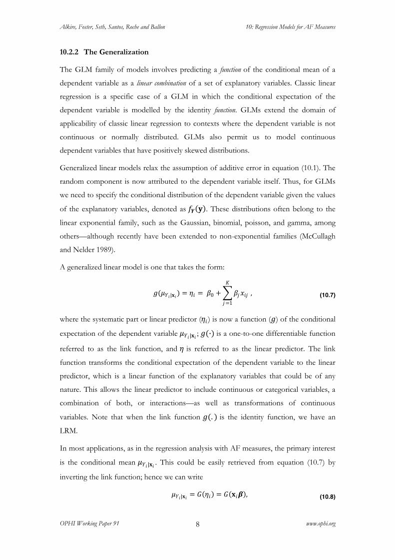
10.2.2 The Generalization

The GLM family of models involves predicting a function of the conditional mean of a

dependent variable as a linear combination of a set of explanatory variables. Classic linear

regression is a specific case of a GLM in which the conditional expectation of the

dependent variable is modelled by the identity function. GLMs extend the domain of

applicability of classic linear regression to contexts where the dependent variable is not

continuous or normally distributed. GLMs also permit us to model continuous

dependent variables that have positively skewed distributions.

Generalized linear models relax the assumption of additive error in equation (10.1). The

random component is now attributed to the dependent variable itself. Thus, for GLMs

we need to specify the conditional distribution of the dependent variable given the values

of the explanatory variables, denoted as 𝑓𝒀 𝐲 . These distributions often belong to the

linear exponential family, such as the Gaussian, binomial, poisson, and gamma, among

others—although recently have been extended to non-exponential families (McCullagh

and Nelder 1989).

A generalized linear model is one that takes the form:

𝑔(𝜇𝑌𝑖|𝐱𝑖) = 𝜂𝑖 = 𝛽0 + 𝛽𝑗𝑥𝑖𝑗

𝐾

𝑗=1

, (10.7)

where the systematic part or linear predictor (𝜂𝑖 ) is now a function (𝑔) of the conditional

expectation of the dependent variable 𝜇𝑌𝑖|𝐱𝑖 ; 𝑔(∙) is a one-to-one differentiable function

referred to as the link function, and 𝜂 is referred to as the linear predictor. The link

function transforms the conditional expectation of the dependent variable to the linear

predictor, which is a linear function of the explanatory variables that could be of any

nature. This allows the linear predictor to include continuous or categorical variables, a

combination of both, or interactions—as well as transformations of continuous

variables. Note that when the link function 𝑔(. ) is the identity function, we have an

LRM.

In most applications, as in the regression analysis with AF measures, the primary interest

is the conditional mean 𝜇𝑌𝑖|𝐱𝑖 . This could be easily retrieved from equation (10.7) by

inverting the link function; hence we can write

𝜇𝑌𝑖|𝐱𝑖 = 𝐺 𝜂𝑖 = 𝐺 𝐱𝑖𝜷 , (10.8)



where 𝐺(∙) is the inverse link 𝑔−1 ∙ , also called the mean function. Equations (10.7)

and (10.8) provide two alternative specifications for a GLM, either as a linear model for

the transformed conditional expectation of the dependent variable—given by (10.7)—or as

a non-linear model for the conditional mean—given by (10.8).

A GLM is thus composed of three components: (i) a random component resulting from

the specification of the conditional distribution of the dependent variable given the

values of the explanatory variables (this is implicit and cannot be seen directly); (ii) a

linear predictor ηi , and iii) a link function 𝑔(. ) (cf. Fox 2008: ch.15).

The distribution of the dependent variable 𝑓𝒀 𝐲 and the choice of the link function are

intimately related and depend on the type of variable under study. The form of a proper

link function is determined to some extent15 by the range of the dependent variable and

consequently by the range of variation of its conditional mean.

In the case of AF poverty measures, we may consider two types of dependent variables

with a different range of variation and distribution. The first type is a binary indicator

identifying multidimensionally poor households. This variable takes the value of one if

the household is identified as multidimensionally poor and zero otherwise. The Bernoulli

distribution is suitable to describe this kind of variable. A typical model in this case is the

probit or logit model. As we will see, in a GLM this is equivalent to choosing a logit link.

The second type of dependent variable that we could study in the AF approach is a

proportion. The Adjusted Headcount Ratio 𝑀0 and the incidence 𝐻 are fractions or

proportions that take values in the unit interval. The binomial distribution may be

suitable as a model for these proportions.

In each of these cases, the link function should map the range of variation of the

dependent variable—{0,1} for the binary indicator and [0,1] for the proportion—to the

whole real line (−∞, +∞). The scale is chosen in such a way that the fitted values

respect the range of variation of the dependent variable. Columns one to five in Table

10.1 present the two types of dependent variables with AF measures that we study in this

section, along with their range of variation, type of model, level of analysis, and random

15 The range of variation of the dependent variable is a mild requirement for the choice of a proper link function. As noted by Firth (1991) this mild requirement is complemented by multiple criteria where the choice of a proper link function is made on the grounds of its fit to the data, the ease of interpretation of parameters in the linear predictor, and the existence of simple sufficient statistics.



variation described by the conditional distribution. The link and mean functions are

explained in the examples in sections 10.3 and 10.4. Before presenting the examples, we

briefly explain the estimation and goodness of fit of GLMs.

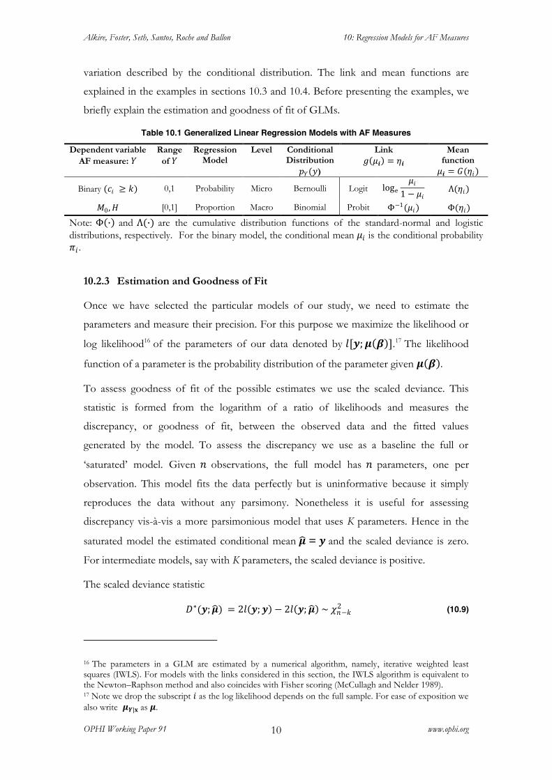
Table 10.1 Generalized Linear Regression Models with AF Measures

Dependent variable AF measure: 𝑌

Range of 𝑌

Regression Model

Level Conditional Distribution

𝑝𝑌(𝑦)

Link 𝑔 𝜇𝒊 = 𝜂𝒊

Mean function

𝜇𝒊 = 𝐺(𝜂𝑖)

Binary (𝑐𝑖 ≥ 𝑘) 0,1 Probability Micro Bernoulli Logit loge𝜇𝑖

1 − 𝜇𝑖 Λ(𝜂𝑖)

𝑀0, 𝐻 [0,1] Proportion Macro Binomial Probit Φ−1(𝜇𝑖) Φ(𝜂𝑖)

Note: Φ ∙ and Λ(∙) are the cumulative distribution functions of the standard-normal and logistic distributions, respectively. For the binary model, the conditional mean 𝜇𝑖 is the conditional probability 𝜋𝑖 .

10.2.3 Estimation and Goodness of Fit

Once we have selected the particular models of our study, we need to estimate the

parameters and measure their precision. For this purpose we maximize the likelihood or

log likelihood16 of the parameters of our data denoted by 𝑙[𝒚; 𝝁 𝜷 ].17 The likelihood

function of a parameter is the probability distribution of the parameter given 𝝁 𝜷 .

To assess goodness of fit of the possible estimates we use the scaled deviance. This

statistic is formed from the logarithm of a ratio of likelihoods and measures the

discrepancy, or goodness of fit, between the observed data and the fitted values

generated by the model. To assess the discrepancy we use as a baseline the full or

‘saturated’ model. Given 𝑛 observations, the full model has 𝑛 parameters, one per

observation. This model fits the data perfectly but is uninformative because it simply

reproduces the data without any parsimony. Nonetheless it is useful for assessing

discrepancy vis-à-vis a more parsimonious model that uses K parameters. Hence in the

saturated model the estimated conditional mean 𝝁 = 𝒚 and the scaled deviance is zero.

For intermediate models, say with K parameters, the scaled deviance is positive.

The scaled deviance statistic

𝐷∗(𝒚;𝝁 ) = 2𝑙 𝒚; 𝒚 − 2𝑙 𝒚; 𝝁 ~ 𝜒𝑛−𝑘2 (10.9)

16 The parameters in a GLM are estimated by a numerical algorithm, namely, iterative weighted least squares (IWLS). For models with the links considered in this section, the IWLS algorithm is equivalent to the Newton–Raphson method and also coincides with Fisher scoring (McCullagh and Nelder 1989). 17 Note we drop the subscript 𝑖 as the log likelihood depends on the full sample. For ease of exposition we also write 𝝁𝒀|𝐱 as 𝝁.



is twice the difference between 𝑙 𝒚; 𝒚 , which is the maximum log likelihood of a

saturated model or exact fit, and 𝑙 𝒚;𝝁 , the log likelihood of the current or reduced

model.

The goodness of fit is assessed by a significance test of the null hypothesis that the

current model holds against the alternative given by the saturated or full model. Under

the null hypothesis, 𝐷∗ is approximately distributed as a 𝜒𝑛−𝑘2 random variable where the

number of degrees of freedom equals the difference in the number of regression

parameters in the full and the reduced models. However, an appropriate assessment of

the goodness of fit is based on the conditional distribution of 𝐷∗(𝒚;𝝁 ) given 𝜷 . If 𝐷∗ is

not significant, it suggests that the additional parameters in the full model are

unnecessary and that a more parsimonious model with fewer parameters may be

sufficient.

The scaled deviance statistic is also useful for model selection. Due to its additive

property, the discrepancy between nested sets of models can be compared if maximum

likelihood estimates are used. Suppose we are interested in comparing two models, A and

B, that represent two different choices of explanatory variables, 𝑿𝑨 and 𝑿𝑩 , that are

nested. Intuitively this means that all explanatory variables included in model A are also

present in model B, a more complex or less parsimonious model. The improvement in fit

may be assessed by a significance test of the null hypothesis that model A holds against

the alternative given by model B. If the value of the scaled deviance statistic is found to

be significant, there is an improvement in the fit of model B vis-à-vis model A, although

a general conclusion on model selection should also consider the added complexity of

model B.

10.3 Micro Regression Models with AF Measures

In the case of micro regression analysis, the focal variable is the (household) censored

deprivation score 𝑐𝑖 . This score reflects the joint deprivations characterizing a household

identified as multidimensionally poor. From a policy perspective a natural question that

arises consequently is how to understand the ‘causes’ that underlie the (multidimensional)

poverty status of a household. The simplest model for this purpose is a probability

model, which we illustrate in this section; although one could also consider modelling the



𝑐𝑖 vector directly. We are thus interested in assessing the probability of a household

being multidimensionally poor. Within the AF framework this is equivalent to comparing

the deprivation score of a household 𝑐𝑖 with the multidimensional poverty cutoff (𝑘). If

𝑐𝑖 is above the multidimensional poverty cutoff (𝑘 ), the household is identified as

multidimensionally poor. This is represented by a binary random variable (𝑌𝑖) that takes

the value of one if the household is identified as multidimensionally poor and zero

otherwise, as follows:

𝑌𝑖 = 1 if and only if 𝑐𝑖 ≥ 𝑘0 Otherwise

. (10.10)

The outcomes of this binary variable occur with probability 𝜋𝑖 , which is a conditional

probability on the explanatory variables. For a (sampled) household 𝑖 identified as

multidimensionally poor this is represented as

𝜋𝑖 ≡ Pr(𝑌𝑖) ≡ Pr(𝑌𝑖 |𝐱𝑖). (10.11)

and thus the conditional mean equals the probability as follows:

𝜇𝑌𝑖|𝐱𝑖 = 𝜋𝑖 × 1 + 1 − 𝜋𝑖 × 0 = 𝜋𝑖 . (10.12)

For a binary model the conditional distribution of the dependent variable, or random

component in a GLM, is given by a Bernoulli distribution (Table 10.1). Thus the

probability function of 𝑌𝑖 is

𝑝𝑌 𝑦𝑖 = 𝜋𝑖𝑦𝑖 1 − 𝜋𝑖 1−𝑦𝑖 . (10.13)

To ensure that the conditional mean given by the conditional probability stays between

zero and one, a GLM commonly considers two alternative link functions (𝑔). These are

given by the quantile functions of the standard normal distribution function Φ−1(𝜇𝑖) and

the logistic distribution function Λ−1(𝜇𝑖)18. The former is referred to as the probit link

function and the latter as the logit link function. The probit link function does not

have a direct interpretation, while the logit is directly interpretable as we discuss below.19

The logit of 𝜋 is the natural logarithm of the odds that the binary variable 𝑌 takes a value

of one rather than zero. In our context, this gives the relative chances of being

multidimensionally poor. If the odds are ‘even’—that is, equal to one—the

18 Note Φ ∙ and Λ(∙) are the cumulative distribution functions of the standard-normal and logistic distributions, respectively. 19 Alternative link functions include the log-log and the complementary log-log links; however, these two are not symmetric around the median.



corresponding probability (𝜋) of falling into either category, poor or non-poor, is 0.5,

and the logit is zero. The logit model is a linear, additive model for the logarithm of odds

as in equation (10.14), but it is also a multiplicative model for the odds as in equation

(10.15):

ln𝜋𝑖

1 − 𝜋𝑖= 𝜂𝑖 = 𝛽0 + 𝛽1𝑥𝑖1+. . . +𝛽𝐾𝑥𝑖𝐾 (10.14)

𝜋𝑖1 − 𝜋𝑖

= 𝑒𝜂𝑖 = 𝑒𝛽0 𝑒𝛽1 𝑥𝑖1 … 𝑒𝛽𝐾 𝑥𝑖𝐾 . (10.15)

The conditional probability 𝜋𝑖 is then

𝜋𝑖 =1

1 + 𝑒−𝜂𝑖=

1

1 + 𝑒− 𝛽𝑗𝑥𝑖𝑗𝐾𝑗=0

. (10.16)

The partial regression coefficients (𝛽𝑗 ) are interpreted as marginal changes of the logit,

or as multiplicative effects on the odds. Thus, the coefficient 𝛽𝑗 indicates the change in

the logit due to a one-unit increase in 𝑥𝑗 , and 𝑒𝛽𝑗 is the multiplicative effect on the odds

of increasing 𝑥𝑗 by one, while holding constant the other explanatory variables. For

example, if the first explanatory variable increases by one unit, the odds ratio in equation

(10.15) associated with this increase is 𝑒𝜂𝑖′

= 𝑒𝛽0 𝑒𝛽1 𝑥𝑖1+1 … 𝑒𝛽𝐾 𝑥𝑖𝐾 , and 𝑒𝜂𝑖′/

𝑒𝜂𝑖 = 𝑒𝛽1 . For this reason, 𝑒𝛽𝑗 is known as the odds ratio associated with a one-unit

increase in 𝑥𝑗 . To see the percentage change in the odds, we need to consider the sign of

the estimated parameter. If 𝛽𝑗 is negative, the change in 𝑥𝑗 denotes a decrease in the

odds; this decrease is obtained as (1 e j )*100 . Likewise if 𝛽𝑗 is positive, the change

in 𝑥𝑗 indicates an increase in the odds. In this case, the increase is obtained as

(e j 1)*100.

10.3.1 A Micro-Regression Example

To illustrate the type of micro regression models that have been discussed, we use a

subsample of the Indonesian Family Life Survey (IFLS) dataset. This is a dataset analysed

by Ballon and Apablaza (2012) to assess multidimensional poverty in Indonesia during

the period 1993–2007. The IFLS is a large-scale longitudinal survey of the

socioeconomic, demographic, and health conditions of individuals, households, families,

and communities in Indonesia. The sample is representative of about 83% of the

population and contains over 30,000 individuals living in thirteen of the twenty-seven



provinces in the country. Ballon and Apablaza (2012) measure multidimensional poverty

at the household level in five equally weighted dimensions: education, housing, basic

services, health issues, and material resources. For this illustration we retain a poverty

cutoff of 33%. Thus a household is identified as multidimensionally poor if the sum of

the weighted deprivations is greater than 33%. That is, 𝑌𝑖 takes the value of one if 𝑐𝑖 ≥ 33% and zero otherwise. Within the GLM framework this binary dependent variable is

estimated by specifying a Bernoulli distribution and a logit link function. This is

equivalent to a logit regression.

The household poverty profile that we specify regresses the log of the odds of being

multidimensionally poor (using 𝑘 = 33%) on the demographic and socioeconomic

characteristics of the household head. For this illustration we use data for West Java in

2007. West Java is a province of Indonesia located in the western part of the island of

Java. It is the most populous and most densely populated of Indonesia’s provinces,

which is why we selected it. The explanatory variables included in this illustration are

non-indicator measurement variables and comprise:

x Education of the household head, defined as the number of years of education (not necessarily completed);

x The presence of a female household head, represented by a dummy variable taking a value of one if the household head is a female and zero if male;

x Household size, defined by the number of household members; x The area in which the household resides, represented by a dummy variable taking

a value of one if the household resides in the urban areas of West Java and zero otherwise;

x Muslim religion, represented by a dummy variable taking a value of one if the household’s main religion is Muslim and zero if not.

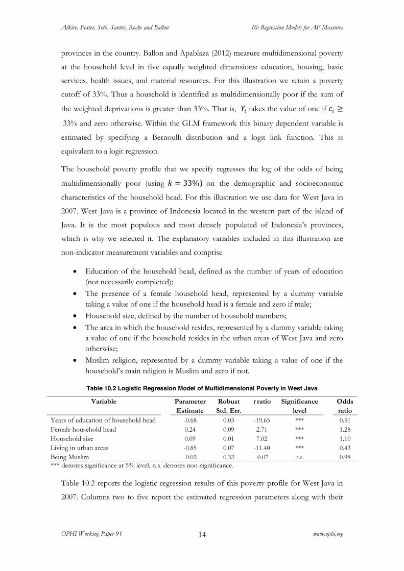
Table 10.2 Logistic Regression Model of Multidimensional Poverty in West Java

Variable

Parameter Robust t ratio Significance

Odds

Estimate Std. Err. level

ratio

Years of education of household head

-0.68 0.03 -19.65 ***

0.51 Female household head

0.24 0.09 2.71 ***

1.28

Household size

0.09 0.01 7.02 ***

1.10 Living in urban areas

-0.85 0.07 -11.40 ***

0.43

Being Muslim

-0.02 0.32 -0.07 n.s.

0.98 *** denotes significance at 5% level; n.s. denotes non-significance.

Table 10.2 reports the logistic regression results of this poverty profile for West Java in

2007. Columns two to five report the estimated regression parameters along with their



standard errors, t ratios, and significance levels at 5%20. Apart from being Muslim, all

other determinants are significant at the 5% level and show the expected signs. For a

given household, the log of the odds of being multidimensionally poor decreases with

the education of the household head and with an urban location and increases with the

presence of a female household head and with household size. The odds ratio for years

of education of the household head indicates that an increase of one year of education

decreases the odds of being multidimensionally poor by 49%, ceteris paribus, whereas

having a female household head increases the odds of being multidimensionally poor by

28%, ceteris paribus.21 Similarly, the odds of a household of being multidimensionally poor

decrease by 57% for households living in urban areas, ceteris paribus, and increase by 10%

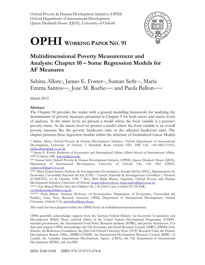
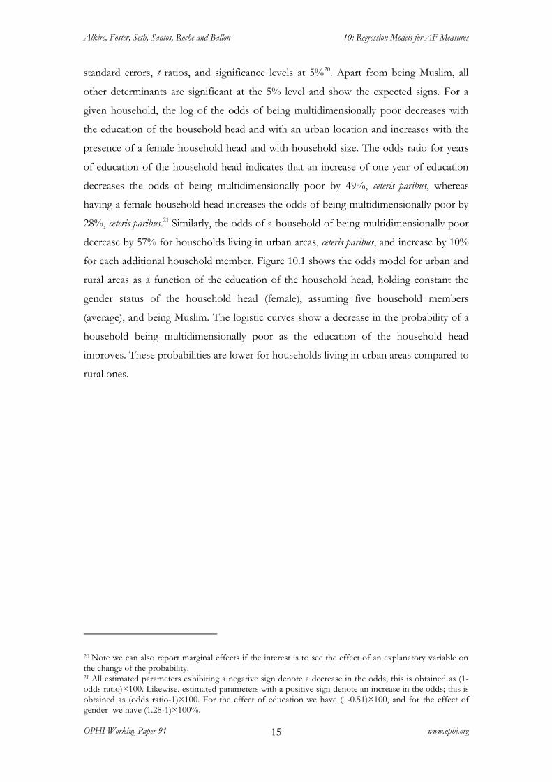
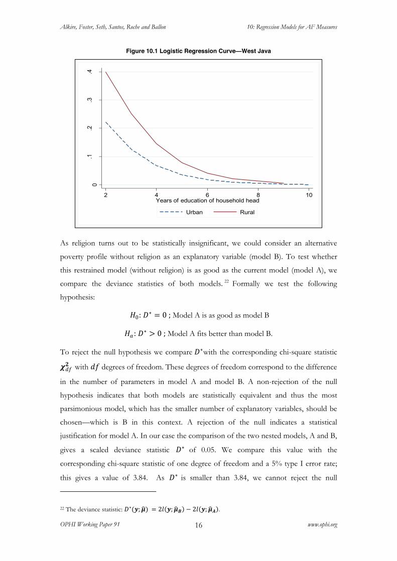
for each additional household member. Figure 10.1 shows the odds model for urban and

rural areas as a function of the education of the household head, holding constant the

gender status of the household head (female), assuming five household members

(average), and being Muslim. The logistic curves show a decrease in the probability of a

household being multidimensionally poor as the education of the household head

improves. These probabilities are lower for households living in urban areas compared to

rural ones.

20 Note we can also report marginal effects if the interest is to see the effect of an explanatory variable on the change of the probability. 21 All estimated parameters exhibiting a negative sign denote a decrease in the odds; this is obtained as (1-odds ratio)×100. Likewise, estimated parameters with a positive sign denote an increase in the odds; this is obtained as (odds ratio-1)×100. For the effect of education we have (1-0.51)×100, and for the effect of gender we have (1.28-1)×100%.



Figure 10.1 Logistic Regression Curve—West Java

As religion turns out to be statistically insignificant, we could consider an alternative

poverty profile without religion as an explanatory variable (model B). To test whether

this restrained model (without religion) is as good as the current model (model A), we

compare the deviance statistics of both models. 22 Formally we test the following

hypothesis:

𝐻0: 𝐷∗ = 0 ; Model A is as good as model B

𝐻𝑎 : 𝐷∗ > 0 ; Model A fits better than model B.

To reject the null hypothesis we compare 𝐷∗with the corresponding chi-square statistic

𝝌𝑑𝑓𝟐 with 𝑑𝑓 degrees of freedom. These degrees of freedom correspond to the difference

in the number of parameters in model A and model B. A non-rejection of the null

hypothesis indicates that both models are statistically equivalent and thus the most

parsimonious model, which has the smaller number of explanatory variables, should be

chosen—which is B in this context. A rejection of the null indicates a statistical

justification for model A. In our case the comparison of the two nested models, A and B,

gives a scaled deviance statistic 𝐷∗ of 0.05. We compare this value with the

corresponding chi-square statistic of one degree of freedom and a 5% type I error rate;

this gives a value of 3.84. As 𝐷∗ is smaller than 3.84, we cannot reject the null

22 The deviance statistic: 𝐷∗(𝒚; 𝝁 ) = 2𝑙 𝒚; 𝝁 𝑩 − 2𝑙 𝒚; 𝝁 𝑨 .

0.1

.2.3

.4

Pred

icted

pro

babi

lity

2 4 6 8 10Years of education of household head

Urban Rural



hypothesis; so we choose the more parsimonious model B and drop religion as an

explanatory variable.

10.4 Macro Regression Models for M0 and H

We now turn to the econometric modelling for the Adjusted Headcount Ratio 𝑀0 and

the incidence of multidimensional poverty 𝐻 as endogenous or dependent variables. As

𝑀0 and 𝐻 are bounded between zero and one, an econometric model for these

endogenous variables must account for the shape of their distribution. 𝑀0 and 𝐻 are

fractional (proportional) variables bounded between zero and one with the possibility of

observing values at the boundaries. This restricted range of variation also applies for the

conditional mean, which is the focus of our analysis. Thus specifying a linear model,

which assumes that the endogenous variable and its mean take any value in the real line,

and estimating it by ordinary least squares is not the right strategy, as this ignores the

shape of the distribution of these dependent variables. Clearly if the interest of the

research question is not in modelling the conditional mean of the proportion but rather

in modelling the absolute change (between two time periods) of 𝑀0 or 𝐻, which can

take any value, standard linear regression models may apply. In what follows we describe

the statistical strategy for modelling the conditional mean of 𝑀0 or 𝐻 as a function of a

set of explanatory variables.

Various approaches have been used in the literature to model a fraction or proportion.

We can differentiate between two types of approaches—often referred to as one-step or

two-step approaches. These differ in the treatment of the boundary values of the

fractional dependent variable. In a one-step approach, one considers a single model for

the entire distribution of the values of the proportion, where both the limiting

observations and those falling inside the unit interval are modelled together. In a two-

step approach, the observations at the boundaries are modelled separately from those

falling inside the unit interval. In other words, in a two-step approach one considers a

two-part model where the boundary observations are modelled as a multinomial model

and remaining observations as a fractional one-step regression model (Wagner 2001;

Ramalho, Ramalho and Murteira 2011). The decision whether a one- or a two-part model

is appropriate is often based on theoretical economic arguments. Wagner (2001)

illustrates this point. He models the export/sales ratio of a firm and argues that firms

choose the profit-maximizing volume of exports, which can be zero, positive, or one.



Thus the boundary values of zero or one may be interpreted as the result of a utility-

maximizing mechanism. Following this theoretical economic argument he specifies a

one-step fractional model for the exports/sales ratio. In the absence of an a priori criteria

for the selection of either a one- or two-part model, Ramalho et al. (2011) propose a

testing methodology that can be used for choosing between one-part and two-part

models. In the case of 𝑀0 or 𝐻 we consider that non-poverty and full poverty, the

boundary values, as well as the positive values, are characterized by the same theoretical

mechanism. This is thus represented by a one-part model. For further references on

alternative estimation approaches for one-part models, see Wagner (2001) and Ramalho

et al. (2011).

10.4.1 Modelling M0 or H

To model 𝑀0 or 𝐻 we follow the modelling approach proposed by Papke and

Wooldridge (1996). For this purpose we denote the Adjusted Headcount Ratio or the

incidence by 𝑦. For a given spatial aggregate, say a country, the Adjusted Headcount

Ratio or the incidence is 𝑦 𝑖 . Papke and Wooldridge (PW hereafter) propose a particular

quasi-likelihood method to estimate a proportion. The method follows Gourieroux,

Monfort, and Trognon (1984) and McCullagh and Nelder (1989) and is based on the

Bernoulli log-likelihood function which is given by

𝑙𝑖 𝜷 ≡ 𝑦𝑖 log 𝐺 𝐱𝑖𝜷 + 1 − 𝑦𝑖 log 1 − 𝐺 𝐱𝑖𝜷 , (10.17)

where 𝐺 𝐱𝑖𝜷 is a known nonlinear function satisfying 0 ≤ 𝐺(∙) ≤ 1. In the context of

a GLM, 𝐺(∙) is the mean function 𝜇𝑌𝑖|𝐱𝑖 defined in equation (10.8) as the inverse link

function. PW suggest as possible specifications for 𝐺(∙) any cumulative distribution

function, with the two most typical examples being the logistic function and the standard

normal cumulative density function as described in Table 10.1.

The quasi-maximum likelihood estimator (QML) obtained from equation (10.17) is

consistent and asymptotically normal, provided that the conditional mean 𝜇𝑌𝑖|𝐱𝑖 is

correctly specified. This follows the QML theory where consistency and asymptotic

normality characterize all QML estimators belonging to the linear exponential family of

distributions, which is the case of the Bernoulli distribution of equation (10.17).



10.4.2 Econometric issues for an empirical model of M0 or H

We would like to conclude with a few recommendations for performing a macro

regression with 𝑀0 or 𝐻 as explained variables. First, we suggest testing for linearity

before specifying a non-linear functional form. For this purpose one can apply the

Ramsey RESET23 test of functional misspecification. The test consists of evaluating the

presence of nonlinear patterns in the residuals that could be explained by higher-order

polynomials of the dependent variable. Second, we recommend testing for possible

endogeneity using a two-stage or instrumental variable (IV) estimation. In regressions of

the type of the macrodeterminants of 𝑀0 or 𝐻, it is very likely that there will be a

correlation between one or more of the explanatory variables and the error term. Let us

suppose we regress the Adjusted Headcount Ratio on the logarithm of the per capita

gross national income in PPP of the same year for a group of countries. This is the GNI

converted to international dollars using purchasing power parity rates. This gives a

contemporaneous model for the semi-elasticity between growth and poverty. In this very

simple model, it is highly likely that the GNI would be correlated with the disturbance of

the equation, which consists of unobserved variables affecting the poverty rate. This

violates a necessary condition for the consistency of standard linear estimators. To deal

with endogeneity, often one replaces the endogenous explanatory variable with a proxy

assumed to be correlated with the endogenous explanatory variable but uncorrelated with

the error term.

Third, one is also very likely to find measurement errors among the explanatory variables

in a model for 𝑀0 or 𝐻. This issue can also be treated with the IV method by replacing

the measured-with-error variable with a proxy. To minimize the loss of efficiency that

may result from an IV estimation, one can complement the estimation results using the

Generalized Method of Moments. Lastly, we would like to point out that although this

Chapter has focused on the modelling of levels of poverty (rates of poverty: 𝑀0, 𝐻), it is

at once straightforward and necessary to analyse changes in poverty. It suffices to estimate

the model in levels and then compute the marginal effects of the expected poverty rate

with respect to the explanatory variables included in the model.

23 RESET stands for Regression Equation Specification Error Test.



Bibliography

Amemiya, T. (1985). Advanced Econometrics. Harvard University Press.

Ballon, P. and Apablaza, M. (2012). ‘Multidimensional Poverty Dynamics in Indonesia’. Paper presented at the Research Workshop on Dynamic Comparison between Multidimensional Poverty and Monetary Poverty. OPHI, University of Oxford.

Barro, R. J. (2003). ‘Determinants of Economic Growth in a Panel of Countries’. Annals of Economics and Finance, 4(2): 231–274.

Bound, J., Jaeger, D. A., and Baker, R. M. (1995). ‘Problems with Instrumental Variables Estimation when the Correlation between the Instruments and the Endogenous Explanatory Variable Is Weak’. Journal of the American Statistical Association, 90(430): 443–450.

De Janvry, A. and Sadoulet, E. (2010). ‘Agricultural Growth and Poverty Reduction: Additional Evidence’. The World Bank Research Observer, 25(1): 1–20.

Dobson, A. J. (2001). An Introduction to Generalized Linear Models. CRC Press.

Dollar, D. and Kraay, A. (2004). ‘Trade, Growth, and Poverty’. The Economic Journal, 114(493): F22–F49.

Firth, D. (1991). ‘Generalized Linear Models’, in D. V. Hinkley, N. Reid, and E. J. Snell (eds.), Statistical Theory and Modeling’. Chapman and Hall.

Foster, J. and Székely, M. (2008). ‘Is Economic Growth Good for the Poor? Tracking Low Incomes Using General Means’. International Economic Review, 49(4): 1143–1172.

Gourieroux, C., Monfort, A., and Trognon, A. (1984). ‘Pseudo Maximum Likelihood Methods: Theory’. Econometrica, 52(3): 681–700.

Haughton, J. H. and Khandker, S. R. (2009). Handbook on Poverty and Inequality. World Bank.

McCullagh, P. and Nelder, J. A. (1989). Generalized Linear Models. (2nd ed.). Chapman & Hall/CRC.

Nelder, J. A. and Wedderburn. R. W. M. (1972). ‘Generalized Linear Models’. Journal of the Royal Statistical Society, Series A 135: 370–384.

Papke, L. E. and Wooldridge, J. M. (1996). ‘Econometric Methods for Fractional Response Variables with and Application to 401(k) Plan Participation Rates’. Journal of Applied Econometrics, 11(6): 619–632.

Rabe-Hesketh, S. and Skrondal, A. (2012). Multilevel and Longitudinal Modeling Using Stata. Volume I: Continuous Responses. (3rd ed.). Stata Press.

Ramalho, E. A., et al. (2011): Ramalho, E. A., Ramalho, J. J., and Murteira, J. M. (2011). ‘Alternative Estimating and Testing Empirical Strategies for Fractional Regression Models’. Journal of Economic Surveys, 25(1): 19–68.

Ravallion, M. (2001). ‘Growth, Inequality and Poverty: Looking beyond Averages’. World Development, 29(11): 1803–1815.

Roelen, K. and Notten, G. (2011). The Breadth of Child Poverty in Europe: An Investigation into Overlap and Accumulation of Deprivations. UNICEF Innocenti Research Centre.

Skrondal, A. and Rabe-Hesketh, S. (2004). Generalized Latent Variable Modeling: Multilevel, Longitudinal, and Structural Equation Models. CRC Press.



Stock, J. H., Wright, J. H., and Yogo, M. (2002). ‘A Survey of Weak Instruments and Weak Identification in Generalized Method of Moments’. Journal of Business & Economic Statistics, 20(4): 518–529.

Wagner, J. (2001). ‘A Note on the Firm Size–Export Relationship’. Small Business Economics, 17(4): 229–237.

Documents

Oxford Poverty & Human Development Initiative (OPHI) · PDF fileOxford Poverty & Human Development Initiative (OPHI) ... Oxford Poverty & Human Development Initiative ... routinely