This book will give ophthalmologists a simple, clear presentation of epidemiologic and statistical techniques relevant to conducting, inter­preting, and assimilating the commonest types of clinical research.

Such information has become all the more important as clinical ophthalmic research has shifted from anecdotal reports and un­critical presentations of patient data to carefully controlled and organized studies.

The text is divided into two parts. The first part deals with epi­demiologic concepts and their application and with the various

types of studies (for example, prospective or longitudinal) and their organization (use of controls, randomness, sources of bias, choice of sample size, standardization and reproducibility). The second half of the text is devoted to the selection and use of the relevant sta­tistical manipulations: determining sample size and testing the sta­tistical significance of results. The text is illustrated with many examples covering topics such as blindness registry data, incidence of visual field loss with different levels of ocular hypertension, sensi­tivity and specificity of tests for glaucoma, and sampling bias in studies of the safety of intraocular lenses. References and several helpful appendices are included.

The Author

Alfred Sommer received his M.D. in Ophthalmology from Harvard University Medical School, and his M.H. Sc. degree in Epidemiology from Johns Hopkins School of Hygiene and Public Health. At the Wilmer Institute, he is the Director of the International Center for Epidemiologic and Preventive Ophthalmology. He is the author of Field Guide to the Detection and Control of Xerophthalmia.

Oxford University Press, N ew York

Cover design by Joy Taylor ISBN O-19-502656-X

Epidemiology and Statistics for the Ophthalmologist

ALFRED SOMMER, M.D., M.R.Se.

The Wilmer Ophthalmological Institute of Johns Hopkins University, and Helen Keller International

New York Oxford

OXFORD UNIVERSITY PRESS

1980

Copyright © 1980 by Oxford University Press, Inc.

LIBRARY OF CONGRESS IN PUBLICATION DATA

Sommer, Alfred, 1942-

Epidemiology and statistics for the

ophthalmologist.

Bibliography: p.

Includes index.

1. Ophthalmology-Statistical methods.

2. Epidemiology-Statistical methods. I. Title.

[DNLM: 1. Epidemiologic methods. 2. Statistics.

W A950 S697 e 1

RE58.S67 617.7'001'82 79-17792

ISBN 0-19-502656-X

Printed in the United States of America

To Nat and Joe

Preface

There are three kinds of lies: lies, damned lies, and statistics.

BENJAMIN DISRAELI

Until recently, epidemiologic and statistical principles were rou­

tinely ignored in ophthalmic research. Fortunately this is no longer

the case, since their use results in better designed, more effi­

cient, and meaningful studies-usually with little additional work.

It is essential that every clinical investigator be familiar with the

concepts involved: where outside epidemiologic and statistical

assistance is available, he must be able to recognize what help

to seek and questions to ask; and where not available, he must

be able to carry out the necessary procedures on his own. It is

equally essential for every informed clinician who wishes to be

better equipped to evaluate the significance and value of pub­

lished -and sometimes conflicting-reports.

This is a practical primer for busy clinicians who have neither

the time nor inclination to pursue formal courses in epidemiology

and statistics. For simplicity and brevity we confine ourselves to

principles and techniques required for conducting and interpret­

ing the most common types of clinical studies: descriptive reports

seeking new etiologic agents, evaluations of diagnostic and

screening procedures, and therapeutic trials.

I can only hope my colleagues will ultimately disagree with

Disraeli, and find the subject interesting and above all, useful.

London, England

September 1979 Alfred Sommer

Acknowledgments

This guide is the outgrowth of what now seems an obvious and

natural merging of my interests in epidemiology and ophthal­

mology. Yet when I originally and quite accidentally considered

combining these two disciplines I encountered little precedent

and even less encouragement. Were it not for Dr. A. Edward

Maumenee, then Director of the Wilmer Institute, and Dr. Abra­

ham M. Lilienfeld, then Chairman of the Department of Epidemi­

ology at Hopkins I would likely have ended up pursuing one of

these disciplines to the exclusion of the other. For their continuing

friendship, advice, and encouragement I am deeply grateful.

I would also like to thank Drs. Frank Newell, Frederick Blodi,

and Argie Hillis for reviewing early drafts and making many help­

ful suggestions, and Mr. David Andrews of the Wilmer Institute

for his editorial assistance.

Epidemiology and Statistics for the Ophthalmologist

Jnten

Epidemiology, 3

Rates: their meaning and use, 3 Attack rate, 3 Relative risk, 5 Group-specific rates, 6 Prevalence and incidence, 7 Sensitivity and specificity, 11 False positives and false negatives, 14

Clinical studies: techniques, common sense, and a few more definitions, 16

Prospective studies, 17 Retrospective studies, 21 Bias and its control, 24

Sampling bias, 24 Randomization, 26 Standardization and adjustment, 28 Loss to follow-up, 29 Controls, 30 Patient bias, 33 Observer bias, 34

Observer variation and reproducibility, 34

The statistical interface, 36 Sample size, 36 Test of significance, 37 Clinical versus statistical significance, 38 Statistical association and epidemiologic inference, .39

Association, 39 Inference, 41

x

Putting it all together, 43 Organization of clinical studies-getting started and staying on track, 44 Is it really \yorth quoting? 44

Statistics, 47

Simple concepts and cookbook formulas, 47 What's it about and why do I need it? 47

Alpha error, 48

Tests of statistical significance, 49 Attribute data, 49

The normal deviate (z), 49 Chi-square (X2), 52

Measurement data, 56

Standard deviation, 57 Standard error, 57 Calculating the standard deviation, 58 Calculating the standard error, 58 Comparison of two independent samples, 58 Comparison of two paired samples, 61 Comparison of three or more samples, 62

Choosing a sample size, 63 Attribute data, 65

Measurement data, 67

Paired samples, 67 Independent samples, 68

Confidence limits, 69

Some parting advice, 72

References, 74

Appendix 1-Table of random numbers, 78

CONTENTS

Appendix 2-Two-tailed probability values for the normal deviate (z), 80

Appendix 3-Probability values for chi-square (X2), 81

Appendix 4-Two-tailed probability values for student's t test, 82

Appendix 5-Background and source material, 83

Index, 84

Epidemiology

Epidemiology has two overriding characteristics: a preference

for rates rather than absolute numbers, and a peculiarly thought­

ful approach to studies amounting to applied common sense .

RATES: THEIR MEANING AND USE

Attack rate

Epidemiologists almost always present data in the form of rates:

the proportion of individuals with a particular disease or charac­

teristic. A common example is the attack rate . Christy and

Sommer ( 1 ) were interested in determining which antibiotic

regimen, if any, offered the best protection against postopera­

tive endophthalmitis . They divided their patients into three

groups (Table 1 ) . The first group received infrequent preopera­

tive topical antibiotics; the second intraoperative periocular peni­

cillin; and the third intensive preoperative topical chloram­

phenicol combined with intraoperative periocular penicillin .

The absolute number of cases in each group tells us little be­

cause the size of the groups varied widely. Absolute numbers

only become meaningful after adjusting for the size of their

respective group . This adjustment, the common attack rate, is

calculated as follows:

3

4

Attack rate

EPIDEMIOLOGY

Number of individuals \vho develop the disease ------------ X 1000

Number of individuals at risk of developing the disease

In each group the "individuals who develop the disease" arc the cases of endophthalmitis, whereas those "at risk of developing the disease" were all individuals who underwent cataract extrac­tion. This adjustment almost always results in a tiny fraction, the number of cases of disease per person at risk. For convenience this is multiplied by 1000 ( or some other appropriate number) and the results expressed as rate of occurrence per 1000 individ­uals. In this particular example it became apparent that intro­duction of combined chloramphenicol and penicillin prophylaxis resulted in a marked drop in the infection rate, whereas penicillin alone had little effect.

Another interesting example is provided by glaucomatous blindness registry data (2). The total number of nonwhites and whites registered as blind in the Model Reporting Area were

Table 1 INCIDENCE OF POSTOPERATIVE ENDOPIITHALMITIS

Infections Prophylactic regimen

Hate Chloramphenicol- Operations per

Series Penicillin sulphadimidine (number) NumiJcr 1000

Ia Jan . '63-Dec. '67 9714 54 5 .6

Ib J an. 'oS-May '72 12,:340 55 4 .. 5

II May '72-Dec. '72 + 2071 9 4.:3

III Jan. '73-March ' 77 + + 21,829 30 1.4

Modifif'd from Christy and Sommer (1).

RATES: THEIR MEANING AND USE

Table 2 PERSONS HEGISTEHED BLIND FROM GLAUCOMA

White Nonwhite

Number

2832 3227

Populationl

32,930,233 3,933,333

1. Fourteen Model Reporting Area states

Rate per 700,0002

8 .6 72.0

2. Population adjusted to a standard (equivalent) age distribution

Modified from Hiller and Kahn (2).

5

roughly comparable (Table 2). Adjusting these numbers for the size of their respective populations, however,

Ratc of registered blindness per 100,000 population

N umber of individuals registered as blind

_...::.s....::..:..:....:...:..-=---.:..:..:..._________ X 100,000 N umber of individuals

in the population

reveals a strikingly different picture: the blindness rate among nonwhites was over 8 times that among whites .

Relative risk

In the example abovc it was natural, almost without thinking, to compare the rate of registered blindness in the two racial groups and thus recognize that the rate among nonwhites was 8 times that among whites . There is a simple term to express this concept : relative risk.

In our previous example, the rate of postoperative endoph­thalmitis among patients not receiving prophylaxis was 4.9 per 1000, while among those receiving combined prophylaxis it was only 1 .4 per 1000. Individuals not covered by combined prophy­laxis ran a risk of postoperative endophthalmitis 4 .9/1.4 or 3 .5 times greater than those receiving combined prophylaxis . Their risk of endophthalmitis, relative to those receiving such �r,��''''_

Iaxis, was 3 .5 : 1 .

6 EPIDEMIOLOGY

_ Rate of disease in group 1 Relative risk

Rate of disease in group 2

Similarly, the relative risk of registrable glaucoma blindness among nonwhites was 8.4 times that among whites.

A "relative risk" is the ratio of two rates : the risk of disease in one group to that in another. It is therefore not an absolute figure. The denominator, of course, assumes a value of 1. Hence the relative risk of the group in the denominator is 1 vis-a.-vis the rate of disease in the group in the numerator.

Similarly, the relative risk for the numerator group is relative to this particular denominator group. If a different denominator group is used, with a different rate (risk) of disease, then of course the relative risk of the group in the numerator will also change, even though its absolute rate (risk) of disease re­mains the same.

Group-specific rates

The rate at which a particular disease occurs within a group is a summary, overall statistic. It does not mean that each and every individual in that group is actually at identical risk of disease. Individuals vary markedly, and some of these differ­ences might be important factors influencing the occurrence of the disease . Our two previous examples make this point nicely . The overall rate of postoperative endophthahnitis among all patients in the series was 3.3 per 1000. This does not mean that all patients ran an identical, 3.3 in 1000 chance of developing endophthalmitis. Slicing up the baloney appropriately, we found that the rate varied from a high of 4.9 per 1000 among those who did not receive prophylactic antibiotics to a low of 1.4 per 1000 for those who received combined prophylaxis . Had we been sufficiently clever in slicing it up further, we might have determined which factors were responsible for endophthalmitis in the first place . As it was, we were not. We classified patients by whether or not they suffered vitreous loss , iris prolapse, extracapsular extraction, etc. and then calculated endophthal·.

RATES: THEIR MEANING AND USE 7

mitis attack rates for each group. Unfortunately, the rates were

roughly the same, the relative risk for each comparison (extra­

capsular extraction versus intracapsular, iris prolapse versus no

prolapse, etc. ) being approximately 1: 1 . Since the relative risks

were all "1", none of these conditions added appreciable risk

to the development of endophthalmitis . They were therefore

not significant risk factors .

The situation with registered glaucomatous blindness was quite

different. The overall rate of glaucomatous blindness was 16 .4

per 100,000. As we've already seen, race-specific rates indicated

that such blindness was more common among nonwhites than

among whites . Race is apparently an important risk factor.

This does not necessarily mean that nonwhites suffer more

glaucoma or have a genetic predisposition to the disease: the

cause may be a lack of health care and delay in diagnosis, greater

access to registration, and the like. We will discuss these epi­

demiologic inferences later.

Race, age, and sex are so often related to disease that their

relative risk almost always requires evaluation. Simultaneous

race-, age- , and sex-specific glaucomatous blindness registration

rates are presented in Table 3. Not surprisingly, blindness rates

increase with age. What is astonishing, however, is 'the extra­

ordinary rate of disease among nonwhites between the ages of 45 and 64. Quick calculation indicates that their risk of glaucoma­

tous blindness registration is 15 times greater than that among

whites of similar age. This does not prove that middle-aged non­

whites are actually more prone to glaucoma or glaucomatous

blindness , but identifies an exceptional event requiring further

investigation. Potential high-risk factors identified in this way are

often the earliest clues to the etiology of a condition.

Prevalence and inc idence

These two terms are almost always misused .

Prevalence is the rate or frequency with which a disease or trait

is found in the group or population under study at a particular

point in time.

8

Se x

Male

Female

E P I D EM I O LOGY

Table 3 RACE-, AGE-, AND SEX-SPECIFIC GLAUCOMA

BLINDNESS REGISTHA TIO;\;S

Rate per 100,000

Age Whi le Non white Ratio nOll white/ whi te

20-44 1.2 9.5 7.9 45-64 9.3 1.54.9 W.7 65-74 42.9 430.2 10.0 75-84 104.5 637.2 6.1

85+ 285.7 707.7 2.5

20-44 0.0 .5.G 9.:3 45-64 8.3 111.1 13.4 65-74 30.9 356.0 11.5 75-84 92 .. 5 5.34.4 5.8

85+ 284.6 773.7 3.1

!'vIodified from Hiller aml Kahn (2).

Number of individuals with the trait

at the time of examination Prevalence = ----:----,--------­

Number of individuals examined

In strict epidemiologic parlance we can say that the prevalence

of elevated intraocular pressures (21 mm Hg or above) in the

general adult population of Ferndale, Wales was 9%, while the

prevalence of glaucomatous field loss was only 0 .4% (3). In less

strict usage, modified for clinical series, we might say the preva­

lence of severe malnutrition among children admitted to the hos­

pital with active vitamin A deficient corneal disease was 66% (4),

and the prevalence of unrecognized intraocular malignant mel­

anomas among eyes enucleated with opaque media was 10% (5).

Prevalence concerns a condition already present at the time of

examination, regardless of when that condition arose .

Incidence is the frequency with \yhich new cases of a disease

or other characteristic arise over a defined pcriod of time:

RATES: T H E I R M EA N I NG A N D USE

Incidence

Number of individuals who developed the

condition over a defined period of time

Number of individuals initially lacking

the condition who were followed for

the defined period of time

9

After the adult population was examined for glaucomatous

visual field loss, ocular hypertensives without such loss were

follmved for ,S to 7 years, and the rate at which new cases of field

loss occurred was calculated (6). On the average, 5 new cases of

field loss occurred among every 1000 ocular hypertensives during

each year of follow-up (an incidence of 5 per 1000 per year ) . In

another with an average follow-up of 43 months, the

incidence of glaucomatous field loss clearly increased with in­creasing level of initial intraocular pressure, confirming the famil­

iar clinical observation that people with higher pressures are at

greater risk of developing visual field loss (Table 4) (7). Prevalence rates and incidence rates are obviously inter­

related. If a condition (such as glaucomatous field loss ) is per­

manent, and if people with it have the same mortality rate as

the rest of the population, the prevalence of the condition in the

Table 4 INCIDE!\CE OF GLAUCOMATOCS \'lSLTAL FIELD

LOSS IN HYPE RTENSIVE EYES

lnitid lOP Total number Developed visual field defect

(mmHg) of eyes number percent incidence!

21-25 75 2 3 8

26-30 25 3 12 34 >30 17 7 41 114

1. Per 1000 per year grossly approximated by applying average follow-up of

4:3 months to all groups . More accurate analysis would have employed an lOP-specific life-table analysis.

Modified from David et al. (7) .

10 EP I D E M I OLOGY

population will be the sum total of its past incidence . Thus, if

the overall incidence of glaucomatous field loss among ocular

hypertensives is 5 per 1000 per year, 50 new cases will occur

among 1000 ocular hypertensives followed for 10 years. At the

end of that period, the prevalence of visual field loss among the

original population of ocular hypertensives will be 50 per 1000.

As usual, life is not always that simple. Individuals with the con­

dition do not always accumulate in the population: the mor­

tality rate among those with the condition might be greater

than among those without, or the condition itself might be

reversible. The overall incidence of active, irreversible, xeroph­

thalmic corneal destruction among preschool Indonesian children

is 4 per 1000 per year (8) . We would therefore expect the

prevalence of corneal scars among five year oids to be about

20 per 1000. Instead it is half that, indicating that the mortality

rate among affected children must have been twice that of the

others. S imilarly, we would expect a large proportion of patients

with intraocular melanoma to succumb to their disease, and the

prevalence of intraocular melanomas in the community to tell

us little about the true incidence of this malignancy.

The prevalence of night blindness and Bitot's spots (potentially

reversible manifestations of vitamin A deficiency) in Indonesian

children is 7 per 1000. This represents the net cumulative effect

of an annual incidence of 10·-14 per 1000 and spontaneous cure

rate of 30-70% (4, 8).

Familiar examples of incidence include the rate of secondary

hemorrhages among patients undergoing different treatments for

traumatic hyphema (although rarely indicated as such, these are

usually new events over a 2-4-week observational period); and

the rate of cystoid macular edema (during the first postoperative

week, month, etc .) following cataract extraction.

These are the rates required to describe most clinical

observations . Does blunt trauma lead to chronic glaucoma?

Simply compare the incidence of new cases of glaucoma among

patients who experienced blunt trauma in the past with the in­

cidence among appropriately matched controls. Alternatively,

compare the prevalence of glaucoma in the two groups at a

RATES: THEIR MEANING AND USE 1 1

particular point in time. Does intraocular lens insertion increase

the risk of cystoid macular edema? Compare the incidence of

CME in matched groups of patients who either did or did not

receive an IOL at the time of cataract surgery over a given

postoperative interval, or the prevalence of CME in the two

groups at one or more postoperative points in time (one month,

one year, etc) . Does miotic therapy reduce the risk of visual

field loss in ocular hypertensives? Compare the incidence of field

loss in two well-matched groups, one treated, one not. As we

shall see, the two groups can be composed of separate individ­

uals , or, preferably, opposite eyes of the same individuals . In every instance we simply compare the rate at which the

disease or characteristic is found (prevalence) or occurs over

time (incidence) in one population to the rate in another. If the

incidence of glaucomatous field loss turns out to be lower in

the miotic-treated group, this group was at lower risk of disease.

How much lower? The incidence in the miotic-treated group,

divided by that in the control group, provides the answer: the

relative risk of field loss in the treated versus the control group .

Sensit iv ity and specif icity

Two additional rates , fundamental to evaluating diagnostic pro­

cedures and criteria, deserve mention: sensitivity and specificity .

As with the rates already discussed (attack rate, prevalence,

incidence, and relative risk) , we are already familiar with the

underlying concepts. When we subject patients with elevated

intraocular pressure to perimetry, tonography, and even long­

term miotic therapy, we do so on the assumption that patients

with elevated intraocular pressure are likely to have glaucoma,

while those with normal pressure are not. Similarly, a vertically

oval cup is said to "suggest" true glaucoma (9 ) . The question,

however, is not whether vertical ovality "suggests" true glaucoma,

but whether it is sufficiently more common among glaucomatous

patients than among normals to serve as a distinguishing charac­

teristic. What we really need to know is the regularity with which

glaucomatous patients have vertically oval cups, and non-

12 E P I DEM I OLOGY

glaucomatous patients lack such cups (10). The former is the

sensitivity of the criterion or test, the latter the specificity.

The sensitivity is therefore the proportion of abnormal individ­

uals detected as being abnormals by the parameter in question

(screen positive):

S . . , Number of abnormals who screen positive

ensltlvlty = --------------�"---­

Total number of abnormals

The specificity is the proportion of normals detected as being

normal (screen negative):

S 'f" Number of normals who screen negative

pecl IcIty = -------:---,,-------:-------:----'=---Total number of normals

Common, shorthand notations for this analysis are given in

Table 5, The sensitivity and specificity of an ideal screening test

would be 100%, a level rarely achieved.

Tonometry is the commonest form of glaucoma screening,

because it is quick and simple to perform, and elevated pressure

is presumed to cause the optic atrophy characteristic of the

disease, Many individuals with elevated lOP, however, never

develop such atrophy. It has therefore become popular to define

glaucoma by the presence of classical visual field loss. With this

Table 5 ANALYSIS OF SCREENING PARAMETERS

Result o f s creeni llg

Positive

Negative

Total

Presen ce o f disease

Yes No

a b c d

a + b + d

S ensitivity = a/ a + c Specificity = d/ IJ + d

False positive rate = b/ a + b + c + d False negative rate = c/a + b + c + d

Total

a + b c + d

a + c+ b+ d

RATES: THEIR MEANING AND USE 1 3

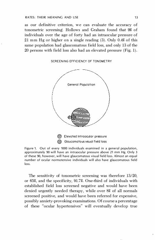
as our definitive criterion, w e can evaluate the accuracy o f

tonometric screening. Hollows and Graham found that � o f

individuals over the age o f forty had an intraocular pressure o f

2 1 m m H g o r higher o n a single reading (3). Only 0.4% o f this

same population had glaucomatous field loss, and only 13 of the

20 persons with field loss also had an elevated pressure (Fig. 1 ) .

SCREENING EFFICIENCY OF TONOMETR Y

Ge neral Papulation

® Elevated Intraoculor pressure

(J) Glaucomatous visual field loss

Figure 1. Out of every 1000 individuals examined in a general population, approximately 90 will have an intraocular pressure above 21 mm Hg. Only 3 of these 90, however, will have glaucomatous visual field loss. Almost an equal number of ocular normotensive individuals will also have glaucomatous field loss.

The sensitivity of tonometric screening was therefore 13/20,

or 65%, and the specificity, 91 .7%. One-third of individuals with

established field loss screened negative and would have been

denied urgently needed therapy, while over 8% of all normals

screened positive, and would have been referred for expensive,

possibly anxiety-provoking examinations . Of course a percentage

of these "ocular hypertensives" will eventually develop true

14 EPIDEMIOLOGY

glaucoma, but the incidence, 1-5 per 1000 per year, is so small,

and drop-out rates during follow-up so high, that keeping track

of such patients may not be worth the effort .

One can frequently improve the sensitivity of a test by lower­

ing the screening criterion, say from 21 mm Hg to 15. U nfor­

tunately, this almost always results in an even more drastic de­

cline in specificity, making the test even less efficient, and often

totally unmanageable.

A valid clinical sign need not always be a useful screening

parameter. By narrowing the criterion, one may raise the specific­

ity dramatically, to a point where any patient fulfilling the cri­

terion has a high likelihood of having the disease (10). For exam­

ple, most patients with an lOP over 40 mm Hg are likely to have,

or soon develop, glaucomatous visual field loss (11, 12) . This is a

useful clinical sign of established or impending glaucomatous

field loss, but this heightened specificity is accompanied by a

marked loss in sensitivity: many patients with the disease would

not satisfy this criterion and therefore would be missed (13) . One of the most important characteristics of the sensitivity /

specificity analysis is that the results are entirely independent of

the actual proportion of normals and abnormals in the study popu­

lation. As can be seen in Table 5, each analysis is column specific:

sensitivity only involves abnormals, specificity only normals .

Such analyses are therefore extremely versatile, and the results

in one population are easily compared with those of another,

even where the proportions of abnormals in the populations

differ. Such is not the case in more traditional false p ositive/false

negative analyses .

False positives and false negatives

The number (or rate) of false positives and negatives depends

not only on the sensitivity and specificity of the test, but also on

the proportion of abnormals to normals in the study population.

As can be seen in Table 5, the analysis is no longer column specific .

In Hollows and Graham's study there were almost 9 false p osi-

RATES: T H EIR M EA N IN G A N D USE 15

tives and 0.2 false negatives for every 100 individuals screened .

This information is not particularly meaningful. Firstly, there is

no way of knowing that fully one-third of all the abnormals had

been missed. Secondly, these false positive and false negative

rates apply only to the distribution of abnormals in this particular

population . If the proportion of abnormals in the population had

been only half what it was, the false negative rate would have

been 0 . 1%, whereas drawing the study population from a con­

sultant's practice (a common event) , where a third or more of the

patients may have established field would a false

negative rate of 11%, even though the sensitivity of test re-

mained UWvHcH"l",'-U

False negative analyses can be used in two other

ways, one useful, the other not. We shall begin with the latter,

the common claim that a diagnosis "was correct 91% of the time."

This i s a summary statistic of little value that conveys even less

information than the actual rate of false positives and negatives .

In analyzing the value of radioactive phosphorus testing for

malignant melanoma, we are interested in learning how many

normal eyes screened positive, and were therefore at risk of

inappropriate enucleation, and how many abnormals eyes

screened negative, and were therefore at risk of going untreated,

and the patient perhaps dying. We don't care that the diag­

nosis was correct 999 out of 1000 times, since that might simply

mean 999 eyes known not to have melanomas (controls) all

screened appropriately negative, while the single case with a

melanoma inappropriately screened negative as well. The result,

99.9% correct diagnosis , sounds extremely accurate, even though

the test was worthless: it was only correct in the huge proportion

of patients never suspected of having a melanoma in the first

place, and missed the single case melanoma in the series

(Fig. 2). False negative rates can be however, in

determining the potential efficiency of a test. The

of tonometric screening, high. It

would be if it were not for the rarity of true glaucoma in the

16

99.9 PERCENT ACCURACY

I Malignant Melanoma

1000 Malignant Melanomas

999 Normals

1000 Test Negatives

p32

TESTER

I Test Negative

999 Test Positives

EPIDEMiOlOGY

Figure 2. 1/99.9% accuracy" is a useless statistic which can mean anything from having missed the only abnormal tested to correctly identifying 999 out of every 1000 abnormals examined.

population. Since only 3% of Hollows and Graham's ocular hyper­

tensives had established field loss, 32 "normals" screened posi­

tive, and would be referred for expensive, potentially anxiety­

provoking evaluation for every 1 abnormal detected, a wholly

unsatisfactory ratio . Results based on our consultant's practice

would appear more efficient because of the higher proportion

of abnormals, hence the higher ratio of true positives to false

positives than would be found in the general population.

C L I N I CA L STU D I ES: TECHN IQU ES, COMMON SENSE, A N D A FEW MORE D EF I N I T I O N S

Most clinical studies fall into one o f two categories : prospec­

tive or retrospective. Despite a common misconception the

CLI N ICA L STUD I ES 17

Table 6

COMPARISON OF PROSPECTIVE AND RETROSPE CTIVE

STUDIE S

Prospective study

Initial disease-free group (A) is

followed over time, and the number

to develop disease (D) and remain

free of disease (C) determined:

A D + C Initial Di-'\'elop('(l Remained

diseasc-free disease free of

,group disease

Attack rate (A.R.) = D/ A

Relative risk of developing disease between two groups, At and Ao (treated and not treated, respectively) is the ratio of their incidence or

attack rates:

Relative Risk {/' A R.t =

Uto A,:Ao

D/A, ----

Do/Ao

Retrospective study

Initial group with the disease (D) and

controls (C) are examined, and the

number tvithout (Do: Co) and with (D,; e,) the trait in question

detemlinecl:

V Do + Dt All individluils Dist'HSP. Disease,

with lh(' \yithol!t with trait

disea<;(' trail

e Co + Ct Controls Controls, Controls,

(no disease) without with trait

trait

Proportion with trait = C/C; D/D

Relative risk of developing disease

between two groups , those with and

without the trait:

Relative Risk

toO = (V,)(Co)

(Do)(C,)

ference between them has nothing to do with when the data are

collected or analyzed . It is far more fundamental (Table 6).

Prospect ive stud ies

A or longitudinal study begins

dividuals free of the disease or trait in

a group of in­

and determines

18 EPIDEMIOLOGY

Table 7 RATE OF SECONDARY HEMORRHAGE IN TRAUMATIC

HYPHEMA

Total Secondary hemorrhage

Regimen (number) number percent

A 66 12 18 B 71 18 25 Total 137 30 22

Modified from Read and Goldberg (14).

the rate at which it occurs over time (Fig. 3). In other words, prospective studies determine incidence; whenever incidence rates are generated, one is dealing with a prospective study. Read and Goldberg (14) found that the rate (incidence) of secondary hemorrhage in traumatic hyphema was not influenced by the treatment regimen (Table 7); Peyman et al. (15) found that the rate (incidence) of postoperative endophthalmitis was signifi­cantly reduced by the use of intraocular gentamycin (Table 8). The collaborative Diabetic Retinopathy Study (DRS) ( 16) showed that photocoagulation retarded the progression of reti­nopathy and eventual loss of vision (Table 9).

In all instances the authors followed two (or more) groups of

Table 8 INTRAOCULAR GENT AMYCIN AND DEVELOPMENT

OF POSTOPERATIVE ENDOPHTHALMITIS

Regimen

Ccntamycin

No gentamyci.n

Total eyes

(number)

W26

400

Modified from Peyman ct al. (15).

Eyes with endophthalmitis

number

6

11

rate/lOoo

3.7

27.5

C L I NI C A L STUD I ES 19

Table 9 CUMULATIVE RATES OF FALL IN VISION TO LESS THAN

5/200 AMONG PATIENTS WITH DIABETIC RETINOPATHY

Therapeutic regimen

Photocoagulation Control

Duration of Rate of Rate of

follou:-uJi No. of eyes visual loss No. of eues visual loss

(mollths) followed (per 100) followed (per 100)

12 ]:588 2.5 ],582 3.8

20 1200 5.3 1 16(-i 11 .4

28 707 7.4 (-i5l 19.6

:36 2:32 10.5 204 26 .5

Modified from The Diabetic Retinopathy Study Research Group ( 16) .

individuals and compared the rates at which an unwanted event

occurred. The greater the difference between the rates, the more

meaningful (clinically s ignificant) it is . The traditional method

of expressing this difference is the relative risk, which in prospec-

tive studies is the ratio of the incidence rates .

Relative risk Incidence of disease in group 1

Incidence of disease in group 2

The rate of postoperative endophthalmitis among patients

denied gentamycin was 3%, versus only 0.4% among those who

received it . Those denied gentamycin had 8 times as much risk of

endophthalmitis as those who received it (3/0.4) . Conversely,

gentamycin reduced the risk of endophthalmitis by 87% (100 -

(0.4/3 X 100) ) .

When prospective data are analyzed during the course o f a

study, it is a concurrent prospective study. All studies above

were of this When, instead, the data are analyzed con­siderably later, often in a manner for which they were never

intended, it is a nonconcurrent prospective Our earlier

example of endophthalmitis rates among postoperative

20 EPIDEMIOLOGY

PROSPECTIVE STUDY

Control Group

Figure 3. A prospective or longitudinal study begins with a group of individ­uals free of the disease or trait in question, who are then followed, over time, for its appearance. In this particular example 25% of the treatment group and 50% of the controls developed the disease (spotted faces) during the follow-up period.

cataract patients was a nonconcurrent prospective analysis of data accumulated over a 15-year period .

A classic, nontherapeutic prospective study was the Framing­ham Heart Study. Smoking habits, serum lipid levels, and a vari­ety of other data were collected on adults being followed for the development of cardiovascular disease . Many years later, another group of investigators took advantage of this accumu­lated data by searching for etiologic factors in the develop­men t of ocular disease ( 17) . Both the heart and eye studies \vere prospective, but the heart study was concurrent because the analysis proceeded along with the accumulation of data; the eye study was nonconcurrent, since the analysis took place years

CLINICAL ST UDIES 21

later and the data liged were not originally collected for that purpose.

Retrospective studies

A retrospective or case control study always contains at least two groups of individuals : one in which all the individuals already have the disease, and a control group in which they do not Instead of being followed over a period of time, they are often examined only once, and the frequency with which different factors or characteristics occur in the two groups compared (Fig. 4 ) . If a factor occurs :nore frequently among abnormals than controls, it is said to be associated with the disease and may or may not be of etiologic significance. A good example is the classic study of histoplasmin skin sensitivity among patients with what we now call presumed ocular histoplasmosis syndrome (18) (Table 10) . The proportion of patients with classical choroidal lesions who had positive skin tests was significantly higher than among pa­tients with other forms of retinal and uveal disease, and the pos­sible role of histoplasmosis in the etiology of the condition strengthened.

A more recent example is the comparison of diabetes rates among patients hospitalized for cataract extraction versus those hospitalized for other reasons (controls ) ( 19) . Diabetes was more common among undergoing cataract extraction

Table 10 HISTOPLASMIN SKIN SENSITIVITY AMOI\C PATIENTS

WITH AND WITHOUT OCULAR "HISTOPLAS:\IQSIS"

Tested Positive Positive (number) (number) (percent)

Classical lesion present 61 ,57 93 Other forms of

retinal-uveal disease 190 48 25

Modified from Van Metre and Maumenee (18).

22 E P I D E M I O LOGY

RETROSPECTIVE STUDY

Figure 4. A retrospective or case-control study always begins with individuals who already have the disease, and a closely matched group who do not. Both groups are examined for the presence of one or more characteristics thought to be associated with (perhaps the cause of) the disease. I n this particular example, 75% of abnormals but only 25% of controls have the trait in question.

Table 11

PREY ALE NCE OF DIABETES AMONG HOSPITALIZED

PATIENTS 40-49 YEARS OF AGE

Reason Total patients Number with Prevalence of hospitalized (number) diabetes diabetes (per 100)

Senile cataract

extraction 60 7 12

Fractures, etc. 1098 30 3

Modified from Hiller ami Kahn (19).

CLINICAL STUDIES 23

1 1 ) , suggesting that diabetics are more likely to undergo cataract

extraction than are nondiabetics . How much more? Unlike the

prospective study, the retrospective study does not produce

incidence or attack rates: the groups are enrolled on the basis

of whether or not they already have the disease. Absence of

incidence data forces us to resort to a more complex, less intui­

tive calculation of relative risk than that used so far (Table 12) .

Retrospective studies are usually less expensive and time con­

suming than prospective ones, but they are also less powerful:

it is more difficult to choose appropriate controls; there is in­

creased risk of hidden bias; and they do not produce incidence

rates . While they can be a useful means of choosing between

several avenues of investigation, design, and analysis are best

left to experienced epidemiologists .

Perhaps the single most important topic in this manual, and

Table 12 RELATIVE RISK OF SENILE CATARACT EXTRACTION

IN DIABETICS CALCULATED FROM RETROSPECTIVE

(CASE-CONTROL) STUDYl

Patient classification

Diabetes present

Cataract extraction ("disease")

yes no

Relative risk (diabetics: controls)

Dt(7) Do (53)

(Dt)(Co)

(Do) (Ct)

(7)(1068)

(53)(30)

= 4.7:1

1. Raw data shown in Table 11.

Modified from Hiller and Kahn (19).

Fracture, etc. ("control")

Ct (30) Co (1068)

24 EPIDEM I OLOG Y

the most intuitive, is the epidemiologist's common sense approach

to study design. Simply stated, it means never losing sight of the

many extraneous factors that can affect a study's outcome .. Fore­

most among them is bias.

Bias and its control

Results are said to be biased when they reflect extraneous, often

unrecognized, influences instead of the factors under investiga­

tion. Potential sources of bias include the choice and allocation

of subjects, their perceptions, and investigator's expectations.

Table 13 lists each of these sources of bias and methods for

their control.

SAMPLING BIAS

Samples chosen for comparison should be as alike as possible

except for the factors under investigation. In a prospective com­

parison of two topical antihypertensive agents for example, the

two groups of ocular hypertensives should differ only in the

Sour ce

Selection bias

Patient bias

Observer bias

Table 13 BIAS AND ITS CO]\;'TROL

114 et hods o f control

E ligibility criteria rigidly fixed and followed Subjects allocated only after enrollment

Randomization

Matching and stratification

Tracing those lost to follow-up

Placebos/ cross-over study

Masking

Firm, objectinc endpoints

Controls

Masking;

Firm, objectivE', well-defined endpoints

Standardization

Measurement of reproducibility

CLI N ICAL STUD I ES 25

medication use. When this is not the case, and the samples

differ in some meaningful, systematic way that influences the

results, sampling bias is present .

Retrospective studies are particularly prone to sampling bias .

In comparing the prevalence of diabetes among cataract patients

and controls the investigators assumed that the two groups were

comparable except for the cataract operation and whatever

etiologic or risk factors were related to it (diabetes) . If they had

been less the controls (fracture patients) might have been

younger than the abnormals (cataract patients). Since the preva­

lence of diabetes increases with age, the prevalence of diabetes

among the cataract group would have been higher than

among controls regardless of whether or not diabetics are more

likely to require cataract extraction.

Other investigators attempted to show, through an unfor­

tunate confusion of retrospective and prospective techniques,

that keratoconus was more likely to follow the use of hard con­

tact lenses than soft contact lenses (20) . They concluded that

the use of hard contact lenses increased the risk of developing

keratoconus . In the absence of careful matching, this was a

hazardous comparison. Many keratoconus patients undoubtedly

become symptomatic from irregular or high degrees of astig­

matism before the true nature of their disease is re·:;ognized.

Since irregular or high degrees of astigmatism require use of

hard instead of soft contact lenses, any general population of hard

contact-lens wearers will automatically contain a higher propor­

tion of future keratoconus patients than a population of patients

using soft contact lenses . In other words the deck was loaded:

use of hard contact lenses was bound to be associated with kera­

toconus, whether or not it contributed to the development of

that disease .

In another analysis, the rate of metastatic deaths among pa­tients who undenvent enucleation for choroidal melanomas (of

all sizes and of invasiveness) was unfavorably compared

with that among patients without enucleation who were followed·

(21 ) . The authors concluded that enucleation was responsible

for the increased mortality in the first group, the fact

26 EPI D EMIOLOGY

that those without enucleation almost invariably harbored small tumors of questionable malignancy.

Sampling bias can also occur in prospective studies, through "bad luck" or the investigator's subconscious bias in recruitment and allocation of subjects. For example, an investigator already convinced of the danger of intraocular lenses in selected con­ditions might unknowingly but consistently assign eyes with significant pathology to the nonimplantation group. Regardless of the true complication rate in the two procedures , the non-10L group would be already weighted with less favorable results .

The same conditions occur when a patient datermines his own therapy, or when two independent series are compared. In a particularly careful, but nonconcurrent, prospective study of the

of intraocular lenses , patients who had received implants at the time of cataract extraction were matched with those who had not, since selection criteria for the implant group had been stricter (22) . Even so, the authors acknowle03ccl at least one potential source of bias : patients with extensive corneal guttata were more likely to undergo routine cataract extraction than intraocular lens insertion. In other words, the two groups had originally differed by more than the choice of operation. Although intraocular lenses were still associated with a higher incidence of postoperative corneal edema, this difference would probably have been even greater had the two series been more

matched .

RANDOMIZATION

Perhaps the greatest virtue of the concurrent prospective study is the availability of a powerful technique for minimizing selec­tion bias : randomization . Randomization ensures that every sub­ject has exactly the same chance of being assigned to each of the study groups . This takes the decision out of the hands of the clinician; it is the only sampling scheme amenable to routine sta­tistical manipulation; and it distrihutes patirnts (on the average) equally between the groups irrespective personal aUributes-

obvious ( like age sex) and unrecognized,

CLI NICAL STUDIES 27

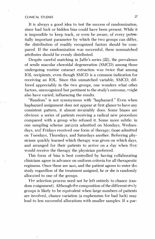
It is always a good idea to test the success of randomization, since bad luck or hidden bias could have been present. While it is impossible to keep track, or even bc aware, of every tially important parameter by which the two groups can differ, the distribution of readily recognized factors should be com­pared. If the randomization was successful, these nonmatched attributes should be evenly distributed .

Despite careful matching in Jaffe's series (22) , the prevalence of senile macular choroidal degeneration ( SMCD) among those undergoing routine cataract extraction was twice that among IOL recipients, even though SMCD is a common indication for receiving an IOL. Since this unmatched variable, SMCD, dif­fered appreciably in the two groups, one wonders what other factors, unrecognized but pertinent to the study's outcome, also have varied, influencing the results.

"Random" is not synonymous with "haphazard." Even when haphazard assignment does not appear at first glance to have any consistent pattern, it almost invariably does. Some biases are obvious: a series of patients receiving a radical new procedure compared with a group who refused it. Some more subtle : in one sampling scheme admitted on Mondays, Wednes­days, and Fridays received one form therapy; those admitted on Tuesdays, Thursdays, and Saturdays another. Referring phy­sicians quickly learned which therapy was given on which days, and arranged for their patients to arrive on a when would receive the therapy the physician preferred .

This form of bias is best controlled by having collaborating clinicians agree in advance on uniform criteria for all therapeutic regimens . Once these are and the patient agrees to enter tt 0)

study regardless of the treatment assigned, he or she is randomly allocated to one of the groups .

ThA selection process need not be left entirely to chance (ran-dom signment) . Although composition of the different groups is likely to be equivalent when large numbers of patients are involved, chance variation (a euphemism for bad luck) may lead to less successful allocations with smaller samples . If a par-

28 E P I D EM I OLOGY

ticular attribute is likely to have an important influence on the

outcome of the trial, the hvo groups can be deliberately matched

for that attribute. For example, we would expect patient age

to influence any comparison of extracapsular and intracap­

sular cataract extraction. Rather than risk the chance that most

of the younger patients will end up undergoing one procedure

and most older patients the other, we can begin the allocation

hy first separating all patients into two strata; those under and

those oyer thirty years of age. The first patient registered in each

stratum is randomly assigned to one of the two operative tech­

niques, the next person in the same age stratum automatically

receiving the other technique. The process is then repeated: the

third patient is randomly assigned to one technique, the fourth

automatically going to the other, etc. Study groups can be matched

on age, sex, race, all three, or any combination of factors that

seems important, although in practice the small number of sub-

jects involved usually limits the number variables on

they can be matched.

Various methods arc availahle for randomizing a series. Per­

haps the simplest is to assign each patient a number from a serial

list of random numbers (Appendix 1). Since every digit has an

equal chance of appearing at every position on the list, there is

no pattern or bias in their arrangement. If the patients are

divided into two groups, those whose random numbers end in

an odd digit go to one group, those with an even digit to the

other. If three groups are involved, patients whose numbers end

in 1, 2, or 3 go to the first group, 4, 5, or 6 to the second, and 7, 8,

or 9 to the third. Random numbers ending in zero are skipped

and not a.igned to any subjects.

STANDARDIZATION AND ADJUSTMENT

'Jespite attempts at randomization, or more commonly where

it was not or could not be used, the different groups (abnormals

and controls, treated and untreated, etc.) might well vary in

ways that could influenci . e outcome. We've already discussed

examples in which a diff.:;I011ce in age distribution, or in the pro-

CLINICAL STUDIES 29

portion of patients with irregular astigmatism, might have and led to biase(}, potentially erroneous results. Proper com­parisons require age-specific or astigmatism-specific analyses, where comparisons are made between subgroups of abnormals and controls of the same age, refractive error, and the like. Alter­natively, when these individual subgroups contain too few cases for comparison, the entire group of abnormals and controls can be adjusted to the same "standard" distribution. Both age­specific and age-adjusted rates were used in the analysis of glau­comatous blindness registry data (see Tables 2 and 3) .

LOSS TO FOLLOW-UP

One of the most common sources of sampling bias, unrelated to the selection process itself, is loss to follow-up. Except for captive populations, all prospective studies will lose patients over time. At best, this only reduces the number of subjects left to work with-the reason we usually recruit more than the number required for purely statistical purposes. At worst, however, loss to follow-up can result in a horribly distorted sample and biased conclusions . In an obvious, if example, any nificant loss to would compromise a com-parison of photocoagulation versus enucleation in the manage­ment of choroidal melanomas. Missing patients merely recorded as "lost to follow-up" may well have died from metastatic disease. If such metastatic deaths occurred in the nonsurgical and the fact that died went unrecognized, photocoagulation would appear safer than it really is (perhaps even safer than enucleation, when the facts might be quite the opposite) .

Good doctor-patient with frequent emphasis on the necessity of remaining in contact with the project tends to min­imize loss to foUo\v-up . Arrangements can be made for have moved outsidc the study area to be followed by a local physician. Even so, SOIne participants will inevitably It is then important to determine whether the rate at which this occurs, and the characteristics of those who have disappeared, varies from Olle study group to another, and, if so, if such vari-

30 EPIDEMIOLOGY

ation is likely to affect the study's outcome. Those who remain in the study should also be compared with those who disappear, and intensive efforts should be made to trace at least a random sample of the missing subjects (by visiting their last known ad­dress , questioning neighbors as to their whereabouts and health status, searching death reports, etc . ) .

CONTROLS

Concerns about randomization, selection bias, and the like all presuppose the use of controls . Except for unusual case reports, any study of substance should be expected to contain suitable controls . The history of our profession is replete with uncon­trolled studies reporting significant therapeutic advances , many of which turned out, on controlled examination, to be no better than placebos. The frequently repeated argument that concur­rent controls were unnecessary to prove penicillin effective in pneumococcal pneumonia is spurious. Few ophthalmic diseases yield so dramatically to a single intervention . More commonly we deal with conditions having highly variable outcomes and treatments providing only a modicum of benefit . To date, there has not been a single well-controlled study demonstrating that photocoagulation benefits patients having presumed ocular his­toplasmosis (POR) or that Daraprim is effective in treating human toxoplasmic chorioretinitis . To the contrary, despite numerous testimonials to the benefit of photocoagulation in POR, recent nonconcurrent comparisons suggest that little is gained from this mode of therapy (23) .

As already noted, controls ideally should match the treatment group in all respects except for the therapeutic regimen. The closer the match, the more meaningful the results. In most in­stances we construct matching groups of individuals , as alike as possible in age, sex, race, and whatever characteristics are peculiar to the disease in question, such as level of intraocular pressure and degree of field loss; size and location of the sub­retinal neovascular net; degree, form, and location of prolifera-

CL I N I CAL STUD I ES 31

tive retinopathy; and size and characteristics of the choroidal

melanoma.

No matter how good the match, it is never perfect. Individuals

always differ. Depending on the size of these differences, this

innate variation, or "background noise," can mask small but

definite therapeutic advantages . In some instances we can elimi­

nate individual variation by matching the two eyes of a single

subject, using a hard contact lens in one, a soft lens in the other;

one form of antihypertensive medication in one, an alternative

form in the other; retinoic acid in one, placebo in the other (24) , etc. But the two eyes of the same individual can differ. Even

this difference can be eliminated by applying first one agent

and then the other to the same eye, a so-called crossover study . A single eye then becomes its own matched control. Examples

include testing various topical antihypertensive agents in the same

eye (25); various carbonic anhydrase inhibitors in the same person

(26); etc. To ensure that the effect of the first drug doesn't in­

fluence the second, different eyes or individuals should initiate

the series with different drugs . By minimizing extraneous vari­

ables (background noise) , these paired comparisons are usually stronger than group (independent) comparisons, and may demon­

strate statistical and clinical significance which might otherwise

be missed.

Nonconcurrent, historical controls are obviously much weaker,

since many other factors (patient selection, operative techniques,

medications, length of hospitalization, etc . ) may change simul­

taneously with the factors under investigation. For example,

traumatic hyphemas treated with a new agent were compared

with those treated many years before (27) . The investigator

acknowledged that many other variables changed in the interim,

but chose to ignore them, attributing all the benefit to the new

agent . The reader might seriously question his conclusions .

Factors that change in the interim need not be obvious. Initial

search of Christy's cataract series identified only a single change

in technique: introduction of periocular penicillin prophylaxis

32 E P I D E M I OLOGY

in May 1972 (ref. 1 and N. Christy, A . Sommer, unpublished data).

The series was therefore divided into two periods, pre- and

postpenicillin. For interest, each subseries was divided further,

at its midpoint. Analysis indicated that there was a drop in in­

fection rates coinciding with the introduction of penicillin prophy­

laxis (Table 14). Surprisingly, however, the rates continued to

decline during the ensuing period. Further investigation revealed

an additional, previously overlooked change: intensive preopera­

tive topical application of chloramphenicol-sulfadimidine was

instituted in January 1973. Dividing the postpenicillin subseries

at this point revealed that penicillin alone had not influenced

endophthalmitis rates in the least. All the improvement followed

the addition of topical chloramphenicol to the prophylactic

regimen (see Table 1). A prospective, concurrently controlled

Table 14

POSTOPERATIVE ENDOPHTHALMITIS AND INTRODOCTIOT\

OF PENICILLIN PROPHYLAXIS

Series

Ia

Jan. '53-Dec . '67

Ib

Jan. '58-May '72

II '\1ay '72-Dec. '74

III

Jan. '75-Dec . '76

Prop hyla cti c peni cillin

+

+

Operations (num ber)

9714

12,340

12,957

10,481

In fections

rate per

numiJer 1000

54 5.6

55 4 .5

30 2.31

9 0.81

1 . Compare with rates shown in Table I , where series II and III are divided at

a different point in time.

"vlodified from Christy and Sommer ( 1 ) and N. Christy, A. Sommer ( lll1published

data ) .

e L i N ICAl STU D I ES

Table 15

INCIDENCE OF POSTOPERATIVE ENDOPHTHALMITIS

IN MASKED RANDOMIZED PROSPECTIVE TRIAL

33

Infections Prophylactic regimen

rate Chloramphenicol- Operations per

Series Penicillin sulfadimidine (number) number 1000

IY + 3309 li5 4 .5

V + + :3.309 5 1 .5

Compare with rates for differing regimens in nonconcurrent series, Table 1.

Modified from Christy and Sommer (1) .

trial then demonstrated that chloramphenicol alone was equally

ineffective, all the benefit arising from combined prophylaxis (Table 15) ( 1 ) .

PATIENT BIAS A patient's expectations can seriously influence the results of

therapy. If he believes that he is receiving the latest, most tech­

nologically advanced treatment (flashing lights, darkened rooms,

and nervous doctors all contribute to his perceptions) he is likely

to experience the greatest subjective improvement. At least two

techniques are useful in controlling this form of bias . The first

is masking. The patient is not told which treatment (if any) he

is receiving . The use of a placebo (or alternative medication)

helps to keep the patient masked. A crossover study, in which

the patient first uses one and then another drug (in masked fash­

ion) achieves the same effect with the additional advantage of

testing two (or more) agents instead of one, with a minimum

of noise. Of course it is sometimes difficult for

placebo or sham regimens to duplicate the conditions of actual

therapy (e .g . , laser burns). The second is reliance on "hard,"

objective e .g . , actual visual acuity or millimeters of

proptosis rather than how the patient "feels . "

34 EP I DEM I O LOGY

OBSERVER BIAS

An investigator's conscious or subconscious (unconscious?) ex­

p ectations can greatly affect a study. We've already discussed

how he can influence the selection and allocation of subjects . He

can also influence the patient's (and his own) p erceptions o f

the benefits of treatment. If already convinced of the value of

a particular mode of therapy, the investigator can always coax

another line from the Snellen chart. Whenever possible, the

person compiling the clinical observations should be masked:

not know whether he is examining an abnormal or control, a

treated or untreated patient. It is obviously impossible to keep

a clinician from knowing that an intraocular lens was inserted

or panperipheral ablation performed. But it is possible to keep

this information from the technician recording best-corrected

acuity or intraocular pressure.

When treatment assignments are masked from both patient

and observer, we have the classic double blind (preferably double masked ) study. Closely related to observer bias is observer

variation.

O bserver var iat ion a n d reproduc i b i l ity

Just as two clinicians examining the same patient may arrive at

different diagnoses, two observers will not necessarily record

the same findings; nor, necessarily, will the same observer examin­

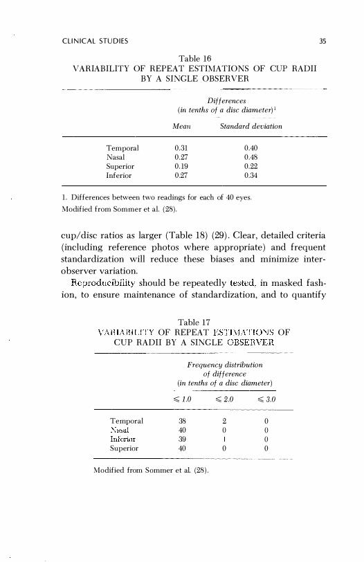
ing the patient a second time. The former is known as inter­observer, the latter intraobserver variation. Forty stereofundus

photographs read twice in masked fashion by the same individual

demonstrated the (intraobserver) variation shown in Tables 16 and 17 (28) . Relatively little can be done to decrease innate vari­

ability of this sort short of switching to other, more objective

criteria .

Interobserver variation is usually greater; the problem is com­

pounded by biases peculiar to each observer. One observer may

be more apt to diagnose cataracts, macular pigment disturbance,

myopic cups, and the like than another, or consistently estimate

C L I N I C A L STU D I ES

Table 16

VAHIABILITY OF REPEAT E STIMATIOI\S OF CUI:' RADII

BY A SINGLE OBSERVER

Temporal

Nasal

Superior

Inferior

Differences (in tenths of a disc diameter) I

!II eall Standard deviation

0.31

0.27

0.19

0.27

0.40

0.48

0.22

0.:34

1. Differences between two readings for each of 40 eyes.

Modified from Sommer et al. (28).

35

cup/disc ratios as larger (Table 18) (29) . Clear, detailed criteria

(including reference photos where appropriate ) and frequent

standardization will reduce these biases and minimize inter­

observer variation.

should be repeatedly in masked fash-

ion, to ensure maintenance of standardization, and to quantify

Table 17

VARIABILITY OF REPEAT ESTIMATIONS OF

CVP RADII BY A SINGLE OBSERVEH

Temporal

�asal

Superior

Frequency distribution of difference

(in tenths of a disc diameter)

,,;; 1.0 ,,;; 2.0 ,,;; 3.0

38 2 0 40 () () 39 () 40 0 0

Modified from Sommer et al. (28).

36 EPIDEMIOLOGY

Table 18 INTEROBSERVER VARIABILITY FOR DIFFERENT CRITERIA

Horizontal C/D < 0.3 Macular pigment disturbance

Myopic cup

Modified from Kahn et al. (29) .

1

78

41

53

Percent of patients diagnosed positive

by observer

2

62

5

2

3

64 19

7

4

43

27

3

5

69

19 o

the magnitude of variation attributable solely to the lack of per­fect reproducibility. Obviously, criteria with firm, quantifiable end points (intraocular pressure) will be far more reproducible than those more subjective and difficult to define (e .g . , presence of a cataract) .

With all their variability, the observers listed in Table 18 worked from a common manual in which all diagnostic criteria were precisely defined . If this is not the case, variability is likely to be much larger . One man's cup (or cataract) is not always an­other's, a major problem in comparing the results of independent studies (or investigators ) .

TH E STAT I STI CAL INTERFAC E

To complete our discussion of epidemiologic principles and study design, we must introduce two major uses of statistics : choice of sample size and tests of "significance ." Both will be discussed in greater detail later. They are the easiest, quickest, most straightforward part of any study.

Sample size

One of the earliest, most important determinations an investi­gator can make is the size of the sample required to test his

TH E STATi ST I CA L I NT E R F A C E 3 7

hypothesis o before the grant application is a single

form designed, a research assistant hired, or patient examined,

he will learn whether the study can be smaller than originally

anticipated, or (more commonly) must be far larger. In fact,

the sample size required may prove so large as to be impracticaL

Better to discover this at an early stage than many frustrating

years later.

Sample size is just as important to the critical reader. Numerous

investigators have reported the absence of a statistically sig-

nificant difference between treatment implying that

they were of efficacy, when the were insufficient

to demonstrate all but the most spectacular of In a study

of unilateral versus bilateral ocular for traumatic

hyphema (30) , the sample size was so small that bilateral patch­

ing would have had to reduce the incidence of secondary hemor­

rhages by over 80% to have had a reasonable expectation of being

proven significant. Since most therapeutic benefits are consid­

erably smaller, it is hardly surprising that the authors found no

statistical difference.

Test of i f i ca n ce

For the it is sufficient to recognize that we commonly employ statistical tests for a single purpose: to determine the like­lihood or that the difference between two

(or more) groups (e. g. , treated versus placebo) might have arisen

purely by chance. The famous notation "p < .05" is simply short­

hand for "the likelihood that we would have observed this large

a difference between the two groups, when in fact there was no

real difference between is less than 5 in 100." When p < the likelihood is even smaller, less than 1 in 100.

convention (nothing sacred or llU'E','"ceOl! begin to consk ,r that some factors other

been for the difference when

being

in

to chance alone is less than 5 in 1000 Our confidence

Hother " i .e . , its statistical increases as

38 EPIDEMIOLOGY

the likelihood of the difference being due to chance recedes (p < .05, < .01 , < .001 , etc . ) .

An important distinction, often overlooked, is that there is ab­solutely no way of proving that a new treatment is beneficial, only that the observed difference is unlikely to have arisen by chance. Conversely, with small samples even large differences can occur purely by chance (e .g . , p < .50 ) . This does not mean that the treatment is not beneficial; only that the possibility of chance producing a difference of this size is so large that it is impossible to demonstrate the "significance" of the treatment effect.

Clin ical vers us statistical significance

In a rush to conform with new scientific standards, many articles conclude that "the differences are highly significant." In regard to what? In most instances the author'means they are statistically significant. Rarely indicated is whether the differences, real or not, are large enough to make any practical difference. An opera­tion that has a success rate of 85% may be statistically significantly better than one with a success rate of 84.6% (that is, the 0.4% im­provement is likely to be real) , but the clinical (or practical) significance is nil (especially since the "superior" procedure may have other mitigating characteristics in cost, complexity, speed, and the like) . Similarly, one drug might heal herpes simplex ulcers in 6.7 days, while a placebo takes 7.0 days . The improvement is real, but is it clinically significant? Fuller Albright was probably expressing this principle when he said of statistical methods : " . . . if you have to use them, I don't believe it" (31 ) . In general, if there is a meaningful difference it should already be obvious. A statistical test of significance merely establishes the risk en­tailed in assuming that the difference was not due to chance. One should examine the level of benefit in light of competing aspects (cost, side effect, etc . ) , before accepting any new treatment as a meaningful therapeutic advance.

T H E STATI ST I C A L I NT E R F A C E 39

Stat i s t ica l assoc iat ions a n d ep idemio logic i n ferences

The goal of most studies is to determine whether two (or more )

parameters are associated with one another. We have seen that

combined prophylaxis was associated with a lower rate of post­

operative endophthalmitis; diabetes with a higher rate of cataract

extraction; and presumed ocular histoplasmosis syndrome with a

higher prevalence of histoplasmin skin-test sensitivity. In each

instance associaiion was statistically the prob-

ability was less than 5 in 100 that it could have arisen chance

alone. VI;!e must now consider why two appear

to be and what inferences and conclusions can be

drawn from that fact.

ASSOCIATION Every association has several possible explanations (Table 19) .

Firstly, the association might not be real : with typical "bad luck"

we may be dealing with one of those 5 in 100, or even 1 in 1000

instances in which the association is due entirely to chance. A

statistically significant event at the .05 level will occur by chance

alon _ once in every 20 observations . This may have been one of

them. , no method is for dealing

forms

When Weber et a1. (32) made 460 comparisons

between viral titers and various

were at risk of

Table 19 POSSIBLE EXPLANATIONS FOR A STATISTICAL

ASSOCIATION

A. Spurious

1 . Chance event

2. Biased study

B. Heal

L Indirect (linked through common third factor)

2 . (possibly etiologic)

mean-

40 EP I D E M I OLOGY

ingless associations . They handled the problem by "deleting

many statistically significant correlations that did not seem sen­

sible. " Investigators studying diabetic retinopathy (16) handled

the problem somewhat differently. Rather than assign prob­

abilities to the apparent associations, they simply reported the

values of the statistical calculations (e .g . , chi-square) . The reader

was provided the opportunity considering the alternatives

for himself .

Alternatively, it may have been bias rather than chance that

caused the spurious association . As already discussed, retrospec­

tive studies have far greater p otential for spurious associations

than prospective studies, since randomization, which leads to

a more uniform distribution of unrecognized but potentially

important factors, cannot be employed.

A ssuming that the association is real, the question still remains

as to whether it is direct, with possible etiologic significance,

or indirect, with two characteristics being linked through their

common association with some third factor. Early in this century

a xerophthalmia epidemic in Denmark was traced to increased

margarine consumption (33) . The association was real but not

really causal . Poorer segments of society had substituted mar­

garine, devoid of vitamin A, for more expensive dairy products .

It was this lack of vitamin A, rather than any toxic substance in

the margarine, that caused the epidemic.

Similarly, trachoma is associated with hot, dry climates . WhGc

the association is real, it is not dir�:;t. D �.ther it is a somewhat

complex interaction between the dry climate, lack of water, and

inadequate personal hygiene, and their effect on trr��mis.sion of

the trachoma agent and contributory conjunctivitis .

To h orrow a classic example from outside the realm of ophthal­

mology, early epidemiologic studies demonstrated that bron­

chogenic carcinoma of the hmg was confined almost exclusively

to men. The association between a person's sex and risk of cancer

was not direct� 'lnd the malignancy not related to male

genes or hormones. Instead, early in the century cigarette smok-

was a male habit and females rarely induXged . was

THE STAT IST I CAL I NTER FACE 41

associated with smoking, and of course smoking was associated with bronchogenic carcinoma. Although the association between maleness and bronchogenic carcinoma was real, it was indirect, through their mutual association with smoking. Just as smoking habits among women have since approached those of men, so has their risk of cancer .

In summary, an association may be spurious or real; if it may be indirect or direct. Numerous methods exist for evaluat­ing the association further: replicating the experiment using dif­ferent populations; employing different, randomized controls; approaching the relationship from a different perspective, using multiple graduated comparisons correlated laboratory ex­periments, etc. For the present, it is sufficient merely to

mind that a statistically significant association can "m n nw "."

many different things .

INFERENCE

An association must be precisely described and no more must be claimed than was demonstrated . A striking error in this regard is the oft-repeated assertion senile cataracts are more common among diabetics than nondiabetics, implying im­paired glucose metabolism is important in the etiology of senile cataracts . In fact, there is little epidemiologic evidence to sup­port this contention. What most studies have shown is that dia­betics are more to undergo cataract extraction than nOll-­diabetics . While the distinction may seem subtle, it has the

est implications (.34). If, in fact, senile cataracts were more common among diabetics, a massive effort should be launched to identify a useful prophylactic agent. Since all we really know is that diabetics have a higher rate of cataract extraction, we must

determine they are at risk of developing a cataract, or only of it removed. It reasonable to <·" ,,·�,�n�

that diabetics are referred to and examined by ophthalmologists more frequently than are nondiabetics, and hence more likely to have their cataracts identified and removed. investiga­tors kept careful sight of what they had actually demonstrated

42 EPIDEMiOlOGY

( diabetics are more likely to undergo cataract extraction) , and

not confused it with what they inferred ( diabetics are at increased

risk of developing cataracts) , the latter, merely an inference,

would not now be established "fact." We did not fall into this trap with an observation already dis­

cussed: the inordinate risk of registerable glaucoma blindness

among blacks . No one claims that blacks are at higher risk of

glaucoma. They might be, but they might also have a more severe

form of glaucoma, be less responsive to medications, make less

use of health services, etc . , or be more assiduous in registering

their blindness than are other segments of society .

Having demonstrated and precisely defined an association that

appears to be real and direct (e .g . , a new therapeutic agent) ,

how widely applicable are the results? No one goes to the trouble

of doing a study just to prove something about those who par­

ticipated in it. The object is to extrapolate the findings to other

peoples and places . VVhen Hiller and Kahn (19) demonstrated

that patients with diabetes were at increased risk of cataract

extraction, they were not just interested in those few patients

studied, but in inferring a fundamental principle about diabetics

in general.

Ideally, a random sample of the entire relevant population

should be studied. In practice, this is rarely feasible. Instead, we

assume u'lat similar persons \vill respond in similar ways . One

must take every precaution, however, to ensure that they are

indeed similar . For example, a history of night blindness proved

to be an effective tool for xerophthalmia screening in Java (35) .

But recognizing and expressing an accurate history of night blind­

ness is probably culturally dependent. There's no guarantee that

it will work equally wen in India. The demonstration that intra­

ocular gentamycin could reduce the incidence of postoperative

endophthalmitis in Indian cataract camps from 3% to 0 .4% does

not mean it will cause any reduction in postoperative endophthal­

mitis in modern, well-equipped hospitals where the rate is al­

ready 0 .1% and the source character of causative agents

are probably different. The first report from the DRS indicated

P UTTI NG IT ALL TOGETHER 43

that photocoagulation was effective in retarding neovascular

proliferation and visual loss (36}-not in all diabetics, nor in all

diabetics with neovascularization, but only in a highly selected

subgroup . Had the patients not been rigidly stratified, the bene­

ficial affects of photocoagulation might have been missed en­

tirely, and even if not, the results may have been inappropriately

applied .

PUTTING IT A l l TOGETHER

Having completed our discussion of epidemiologic principles and techniques, we should pause for a brief review. As stated

at the outset, epidemiology is characterized by a preference for

rates ( summarized in Table 20) , rather than absolute numbers,

1. Attack rate

2. Incidence

3 . Prevalence

4. Relative risk

(retrospective study)l

5 . Sensitivity

6. Specificity

Table 20 BASIC RATES

number who develop attribute

number followed

number who develop attribute over specified period of time

number followed for specified period of time

number with attribute

number examined

incidence in group 1

incidence in group 2

prevalence in group 1

prevalence in group 2

number of abnormals screening abnormal

total number of abnormals

number of normals screening normal

total number of normals

1. Only in special instances. True relative risk requires the more complex analysis shown in Table 6.

44 E PIDEMIOLOG Y

and a particularly thoughtful approach to the conduct and inter­

pretation of studies . More detailed discussions of epidemiologic

principles and techniques can be found in references E-l through E-5 of Appendix 5.

Organizat ion of cl inical stu d i es-getting sta rted

and stay ing on track

All clinical investigations adhere to Murphy's law: "Everything

that can go wrong, will ." It operates at every step and phase of a study, the potential for problems (especially in the critical

areas of selection, patient and observer bias) increasing geomet­

rically with the number of investigators, and exponentially with

the number of centers involved.

Although Murphy's law can never be fully circumvented, care­

ful attention to detail will minimize its impact. Some of the more

critical steps in planning and executing clinical studies are sum­

marized in Table 21 .

Is i t rea l ly worth q u ot ing ?

Whereas the investigator's job is to reduce the impact of Murphy's

law the reader's job is to identify every instance in which he

failed . Before all else, the reader must satisfy himself that a study

was conducted and interpreted properly and that its conclusions,

regardless of how dramatic and potentially important they seem,

are likely to be valid. This is only possible where study methods

are described in sufficient detail for critical evaluation. Where

they are not, the reader must be wary of accepting the results .

Table 21 highlights areas where most mistakes occur and to

which the reader should pay the greatest attention. Was the

sample size really adequate to disprove the value of the drug

or procedure, and at what level of potential benefit ( 10% or 80%)?

Were the observers adequately masked and standardized, and

how large was the interobserver variation? Were techniques for

allocating patients and investigating those lost to follow-up suf-

PUTT I N G IT A L L TOGET H E R 45

Table 21 CHlTlCAL S TEPS IN A CLINICAL STUDY

Step

1, Define specific goal(s)

2. Review literature thoroughly

3. Select sample size

4. Establish, standardize, and quan­tify reproducibility of forms, pro­

cedures, and personnel before start­

ing study (pilot trial) and at frequent intervals thereafter

5. Prepare detailed protocol

6. If therapeutic trial, every patient

meeting criteria is offered par­

ticipation. Only after they accept

are they randomized.

7. If case-control study, examinc

matching carefully to rule out in­

appropriate or biased controls

8. Repeatedly check monitorable data

(age, sex, race, etc. ) between

groups to ensure randomization

(if applied) is functioning properly .

9. Deterllline whether masking re­

effective .

10. Conduct repeated, specific

Comment

Diffuse fishing expeditions often get nowhere

May discover question already an­

swered, bctter ways to design study,

other areas worth considering, and background data required to determine

sample size.

May need lllore or fewer patients than

originally anticipated. Required sample

size may prm·c so large that study is

impractical

Poor, unreproducible questions and

procedures can be modified or re­

placed without loss of study data; mag­

nitude of intra- and interobserver vari­

ation must be known for analysis of

results.

Ready reference of al l procedures; and

basis of "intwcluction,'· "methods," and

"discussion·· sections in final report.

Randomization hefore enrollment in­

troduces potential bias.

Selection of controls most critical part

of study; can easily result in biased

sample and results.

A breakdown of randomization can occur at any time.

If code inadvertently broken, observa-

tions may biased.

If bias is d iscoyered

completed, study

able .

Oll h" after study

not be salvage-

46 EPIDEMIOLOG Y

Table 2 1 (cont . )

Step

1 1 . Review cases lost to follow-up for consistent pattern that might ex­plain results. Where possible, trace a random subsample to establish definite outcome.

12. Where indicated, subject all results to rigorous statistical tests .

13. Estimate clinical, as well as statis­tical, significance of results

14. Consider alternative explanations for any apparent associations.

15. Inferences should be strictly grounded in actual observations .

Comment

Patients lost to follow-up represent a potentially important source of selec­tion bias.

Required to prove point and necessary for publication. But do not disregard obvious or potential differences just because they are not statistically signifi­cant. Sample size may simply be too small because of error in original assumptions.

The two are not synonymous and should not be confused.

Not all associations are real, meaning­ful, or of direct, etiologic or therapeutic significapce.

The greater the distance between in­ference and actual observation, the more hypothetical and less meaningful the inference.

ficient to rule out sizeable selection bias? Could the degree of

patient, observer, or selection bias account for the results? Were

all reasonable explanations for apparent associations explored

or only those the author originally hypothesized? Were the au­

thor's conclusions warranted by his data, or did his inferences

wander far afield? Passing muster with a journal's referees is

no guarantee that an article proves what it claims (37-39) .

Stat i st i cs

S I M PLE CONCEPTS AND COOKBOOK FORM U LAS

Statistics are a rather simple matter, at least as regards the vast

majority of clinical studies; they are absolutely critical to any

well-designed study with the least of pretensions; and they have

become a rather practical necessity as the better journals begin

to impose a semblance of science on our communications .

What's it about and why do I need i t?

Statistics are simply a means of expressing probabilities. Why

bother? Because we never deal in absolute truths (a probability

of 1 .0 ) , or at least we need some way of recognizing how close

we come to them. In the commonest example, we wish to know

whether a difference observed between two groups, say the rate

.of postoperative endophthalmitis or histoplasmin skin test sen­

sitivity, is real and likely to recur in repeated experiments, or simply the result of chance variation-likely to vary from ex­

periment to experiment and disappear entirely when averaged

over repeated investigations . If a hundred people flip the prover­

bial coin 10 times, they will, on the average, end up with 5 heads

and 5 tails . While true of the average, this is not true for every

individual person. We'd be very surprised indeed if some people

47

48 STATISTICS

didn't get 6 , 7 , 8, or even occasionally 10 heads on the basis of chance variation, although intuitively we recognize that the greater the deviation from the average, the less frequently it should occur. One person in one hundred tossing 8 heads and 2 tails is not inconsistent with an expected average 5 :5 split, al­though ten out of the same hundred people would a crooked coin tossers ) . Before the coin's owner in

we might ask a statistician how often this many large deviations from the expected 5:5 split would occur on the basis of chance alone. The statistician might say that this is an uncommon event, which should occur less than 5% of the time

< .05) . That if we repeated the experiment 100 each time having the same one hundred people toss the coin 10

we might ten honest to toss 8 or more heads in less than 5 of those 100 experiments . A law-and-order judge might consider that occurrence so unlikely as to prove the fellow's guilt. But an appeals court might overturn the verdict, arguing that 5 in 100 is too frequent to dismiss the possibility that it was

to chance and only if its likelihood of occurring chance were less than 1 in 100 < .01 ) , or 1 in 1000 (p <

.001 ) should the coin's owner be convicted of fraud . Our usual, run-of-the mill statistical tests are therefore simply a

means of determining the likelihood that our observations could have occurred by chance alone. Conversely, when the likelihood

their being � event is 11, we consider the results a difference between two to be real, i . e . ,

ca " . For no very reason historical event with less than a 5% probability of occurring chance alone (p < .05) is routinely accepted as statistically significant. We feel even more confident, however, if the likelihood of a chance oc­currence is even low�. (e .g . , p <

A l p h a error

Whenever we "accept" an observation as a real occurrence, we do so at risk of being wrong: regardless of how unlikely it is to

TESTS OF STATISTICAL SIGNIFICANCE 49

have arisen from chance alone, it always could have . If P is less than .05, the risk is 1 in 20 that an observation which is not real (e .g . , the difference between two treatment effects) will prove statistically significant. This risk of being wrong and accepting an observation as true when in fact it was merely due to chance, is known as the alpha error. Almost all statistical tests present their "level of significance" in terms of the alpha error.

TE STS OF STATIST ICAL S I G N I F I C A N C E

In usual clinical practice we wish to compare observations in one group of individuals with those in another, and determine whether any apparent differences are likely to be real ( i . e . , were they unlikely to be due to chance). Choice of an appropriate statistical test depends, for the most part, on whether we are comparing attribute-type data (the proportion of individuals who went blind, developed nerve fiber bundle defects, had re­lapses, etc. ) or measurement-type data (average number of days to corneal healing, mean intraocular pressure, etc. ) .

Attri bute data

Here we are dealing with the proportion of individuals with a particular attribute ( the rate at which a characteristic occurs in two groups of individuals ) .

THE NORMAL DEVIATE (z) PI is the proportion of individuals in the first group who have that attribute, P2 the proportion in the second.

number of individuals with the attribute P

number of individuals examined in that group

n - the number of people in that group

q 1 - P = the proportion of individuals in the group with­out the attribute

50

p = average proportion positive in the 2 groups

nIPl + 1I2P2

ni + 112

STATISTICS

q 1 - P = the average proportion negative in the 2 groups

The general formula is :

The resultant number z is known as the normal deviate. The prob­ability that the difference between the groups (PI - P2 ) could have arisen by chance is shown in tables of normal deviates op­posite the appropriate z value. It is always safest to use a "two­tailed test," since Pl could be either larger or smaller than P2 . A two-tailed table of z is provided in Appendix 2 .

A quick glance at the formula reveals two obvious facts:

1 . The larger the difference between PI and P2 , the larger the z value

2 . Similarly, the larger the size of the two groups (nl and 112) the larger z

The larger z is, the less likely is the possibility that the observed difference is due to chance alone (Le . , the more statistically significant it is) .

In practical terms, this means that large differences require fewer patients to prove statistical significance, whereas smaller differences require larger samples . Once again, a sufficiently large population can establish statistical significance for a very small difference, even one that is not the least bit "significant" from a clinical standpoint. Conversely, too small a sample can mask a moderate though clinically meaningful difference.

Illustrative example: The prevalence of superficial punctate keratopathy (SPK) among patients with conjunctival xerosis was

TESTS OF STATISTICAL SIG NIFICAN CE 51

75% and among controls 7% (40 ) . Is the difference statistically

significant?

n number

with SPK p

q

15

Group 1 Conjunctival xerosis

Group 2 Controls

63 58

47 4

47/63 = .75

1 .00 - .75 = 0 .25

4/58 = .07

1 .00 - .07 = 0 .93

47 + 4

121 = 0.42

1 . 00 - 0.42 = 0.58

Test: z = _-;=P:=I,=;=:=-====P2==:=7'

Vpq(:1 + �) 0.75 - .07

(0.42 ) (0 .58){;3

+ ;8)

= 7.6

Looking up the z value of 7 .6 in Appendix 2, we find it completely

off the table, indicating P < .001 . Had the z value been only

1 .97, P would have been < .05. If z had been 2.8, P would have

been < .01 .

A small bit of complexity might be added at this point. This

particular test of significance requires a "correction for con­

tinuity," especially if n < 50. What that means is unimportant.

What you must do is narrow the difference observed between

the two groups slightly, by subtracting 0.5 from the numerator

used in arriving at P of the larger proportion, and adding 0 .5

to the numerator used in arriving at p of the smaller proportion .

Assuming PI > P2 , the corrected formula is:

52

Zc

( 0.5) ( 0.5\ PI - -;- - \P2 + -;;;)

vpq(� + �) n1 n2

STAT I S T I C S

In general I find the normal deviate to be a more useful test than chi-square, because it deals directly with the rates or pro­

portions in which we are interested. The on the other

hand, deals \vith absolute numbers, which have little inherent

meaning. The statistical basis of the two tests, however, is

identical.

The normal deviate (z) test is not

lo\ving circumstances:

under the fol-

1 . Where the size of the sample is small (n < 20 or larger­

between 20 and 40-but the smallest number with the attribute

is less than 5) employ Fisher's exact test (S-l and S-2, Appen­

dix 5) .

2. To determine the likelihood that the proportion of individuals

with the attribute in three or more groups was due to chance,

rather than comparing one group with another, we use the

chi-square test.

CHI SQUARE ()(2) As noted, )(2 is statistically equivalent to the z test. It

also has the same "small sample" limitations . For our purposes

its sole advantage is the ability to compare attribute data in three

or more groups .

We begin by calculating the overall distribution of individuals

with and without the attribute in the study as a whole, and then

the degree to which the distribution within each group differs

from the distribution. The chi-square test determines the

probability that this ( cumulative) amount of variation could have

arisen by pure chance. If the probability is low < .05 , P < . 01 , etc. ) , we conclude that one or more of the groups differs from

the others in some meaningful way. To determine which groups

TESTS OF STATIST I CAL SIGN I FI CANCE 53

(and how many) differ, we can resort again to simpler two­

group (z) comparisons . . The general formula for chi-square is as follows :

where

L (f - F )2

F

f = the number of individuals observed to have (or not have)

the attribute in that group

F = the number of individuals expected to have (or not have)

the attribute in that group ( if the overall proportion of

people with and without the attribute in the study as a

whole applied)

L = sum of the calculations for all of the groups

In longhand, we say X2 is equal to the sum of the square of the

difference between the observed and expected frequency di­

vided by the expected frequency in every group.

Our first task is to construct a contingency table, simply a con­

venient means of displaying the data. As an example we will use additional data from the study on prevalence of punctate kera­

topathy among children with clinical xerophthalmia. Alterna­

tively, one could be dealing with incidence of visual loss among

patients on various antihypertensive medications, with various

degrees of diabetic retinopathy, etc .

F our groups of children were studied: normals , and children

with night blindness, conjunctival xerosis, or corneal xerosis .

The observed number ( f ) of children with and without punctate

keratopathy in each group is shown in Table 22. This is known

as a 2 X 4 contingency table, since it distributes the entire study

population among two classes (rows) and four categories (col­

umns) , resulting in eight "cells ."

Next, we determine the expected number (F) of individuals

in each cell. The expected number is derived by applying the

overall distribution of positives and negatives to the total number

54 STATISTICS

Table 22 CO:\TINGENCY TABLE Al'\ALYSIS

I. Number of Eyes Observed (f )

Corneal Conjunctival Night Nornwl SPK xerosis xerosis blindness controls Total

Present 47 47 10 4 108 Ahsent 0 16 III 54 88

Total 47 63 28 58 196

of children in each of the four groups. A simplified formula for determining F for any cell is :

F = ( row total) ( column total)

grand total

Note that if one carries out this calculation for a single cell in each of three different columns, the five remaining cells can be computed by simple subtraction. Results are shown in Table 23'.

The difference between the observed and expected numbers (f - F) in each cell appears in Table 24. To calculate x2 we sim­ply plug in the appropriate numbers :

x2 = (f - F ) 2 _ (21 . 10)2 + (-21 . 10)2

F 25,90 21 . 10

+ ( 12,:'9)2 + (-12.29)2 34. / 1 28.29

(-5.43)2 (5.43)2 +

15.43 +

12.57

+ (-27.96) 2 +

(27.96 ) 2 31 .96 26. 04

= 106 .26

We now have the value for X2 • What in the world do we do

TESTS O F STAT IST I CAL SIGNI FICANCE

SPK

Present Absent

Total

Table 2:3 CON1T\GENCY TABLE ANALYSIS

II. Number of Eyes Expected (F)

Corneal Conjunctival Night Norrnal xerosis xerosis blindness controls

25.90 34 .71 15.43 31 .96 21.10 28.29 12 .. 57 26.04

47.00 63.00 28.00 58.00

Table 24 CO"ITIl\GENCY TABLE Al\ALYSIS

III. Number of Observed Minus Number Expected (f -

Corneal Contunctival Night Normal SPK xerosis xerosis blindness controls

Present 21 . 10 12.29 -5.4.3 -27.96 Absent -2UO -12.29 5.43 27.96

55

Total

108.00 88.00

196.00

with it? Simply tum to Appendix 3, a table of probability values for x2 • This is used in much the same way as the two-tailed table of z except for one added annoyance: you must choose from a column labeled of freedom" (d .f. ) . Whereas the involved is not germane to our discussion, choosing the correct degrees of freedom is. This is simply calculated from our con­tingency table :

d .f . = (number of rows - l ) (number of columns - 1 )

In this particular example, we were U v ' U R H ' .... with a 2 X con­table, hence

d .f . = (2 - 1 ) (4 - 1) = 3

and the p value for our study, with X 2 of 106 .62, and 3 d .f . is <

56 STATISTICS

Table 25 CHI-SQUARE FOR 2 X 2 TABLE

Simplified Version Already Employing Yates Correction

I . Format of table

Column Column I II Total

Row I a b rj Row II e d r2

Total kj k2 N

II. Simplified formula for X� N( lad - bel - J�N ) 2

XE = -----'-----'---'-

(kj )(k2)(rj )(r2 )

where ( lad - bel - J�N ) indicates reducing the absolute value of ad - be by one-half the sum of the observations (N) .

. 001 . We really do not have to prove this when the differences are as large and obvious as in this case.

The good news is that the x 2 test can be used even if some

values of F (expected number) are as low as 1, as long as most

are substantially larger (at least 5); and that when x 2 has more

than 1 dJ . , the "correction for continuity" (necessary in the z, or its equivalent , the 2 X 2 X2 test) is unnecessary .

If you insist on using the X 2 test instead of the normal deviate

(z) , it is always safest to employ the Yates correction factor.

This is already incorporated in the simplified determination of

x 2 applicable to 2 X 2 contingency tables shown in Table 25.

Measu rement d ata

Statistical tests of the difference between measurement data ( dealing with means instead of proportions) in two groups are

a bit trickier; they require familiarity with two additional con-

TESTS OF STATISTICAL SIG NIFICANCE 57

cepts: standard deviation (of the observations ) and standard

error ( of the mean) . Neither is particularly complex.

STANDARD DEVIATION

If we were to measure the intraocular pressure of 100 eyes ran­domly selected from the general population, we would find that

they varied considerably. The lowest measurement might be 8,

the highest 32, and the remainder somewhere in between. The

mean, calculated by adding all the measurements together and

dividing by the total number of eyes examined ( 100 in this in­

stance) would be about 16 . The standard deviation ( S .D . ) is

simply a technique for indicating the degree of variation of the

individual measurements about this mean. The mean ±1 S .D .

would include two-thirds of all the individual measurements. A

common standard deviation of lOP among normal eyes is 2 .4 .

Therefore, 66!#; of the population measured would have an lOP

within the mean ±1 S .D . (Le . , 16 ± 2.4; 13.5-18.4 mm Hg) . The

mean ±2 S .D . encompasses 95!#; of all measurements . So 95!#; of

the individuals in the group have an lOP between 16 ± 2 S .D .

( 16 ± 4.8; 1 1 .2-20 .8 mm Hg) . In fact, this i s exactly the way 21

was chosen as the standard upper limit of "normal" lOP. Not

because there is anything magic about 21 , but because over 95!#;

of the general population has a pressure equal to or below this amount.

STANDARD ERROR

The standard error of the mean ( S .E . ) relates not to the variation

of individual measurements about the mean for that particular study or group, but the variation of mean measurements, each

from a different s tudy, about the mean for all the studies . For

example, the mean lOP for the first examination of 100 eyes

might be 16 .5 . The second series of measurements on the same

eyes might have a mean of 17.4, and the third 15.9. The standard

error of the mean (S .E . ) would describe the variation of these

individual study means ( 16 .5, 17.4, and 15.9) about the mean

for all three studies together ( 16 .6 ) . It should be intuitively ob-

58 STATISTICS

vious that the variation of sample or study means about the "true" mean ( i. e . , the mean of all the samples or studies together) will be smaller than the variation of individual measurements about a single study's mean . Since each study's mean has already aver­aged out the extreme highs and lows of the individual measure­ments within that study, study means are less likely to vary by a large amount from one another, or the overall mean. As with the S .D . , the overall sample mean ±l S .E . will include two-thirds of all individual sample means, and the overall sample mean ±2 S .E . will include 95%.

CALCULATING THE STANDARD DEVIATION

For years, students of elementary statistics have memorized the formula for the standard deviation. This is no longer necessary, and it will not be given here . Almost any inexpensive electronic calculator can do it automatically, and with greater precision and ease than was previously possible.

CALCULATING THE STANDARD ERROR

Unlike the standard deviation, which is calculated directly from the actual observations of which it is composed, the standard error is rarely determined from multiple replications of the same experiment. Since the S .E . is always smaller than the S .D . , and to a reasonably predictable degree, it is calculated directly from the S .D . as fo11ovv5:

S E = S .D .

. . vn where n = the total number of observations from which the S .D . was calculated.

COMPARISON OF TWO INDEPENDENT SAMPLES

\Vith a simple calculator in hand, we can now determine whether the difference in measurement data (e .g . , lOP) between two samples is statistically significant.

1. For each of the two samples, calculate its mean (x) , standard

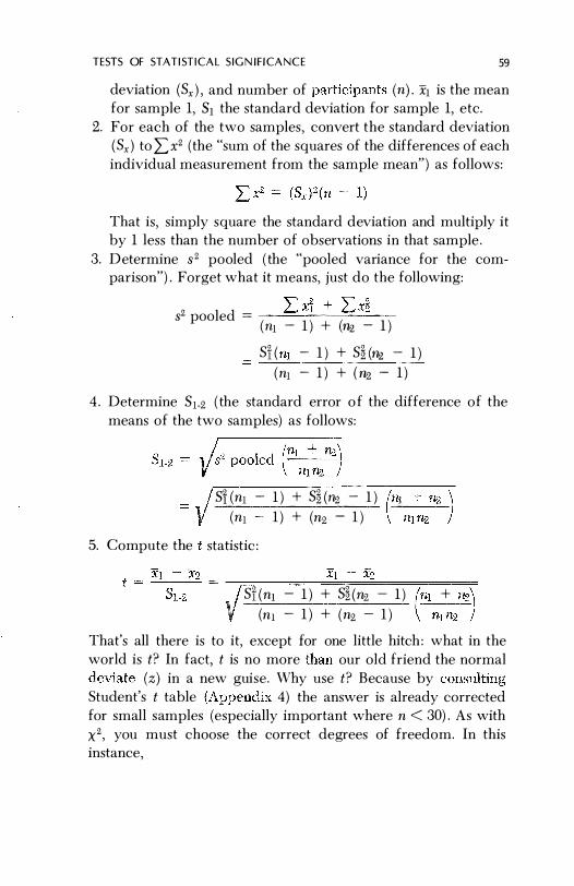
TESTS OF STATISTICAL SIGN i f i CANCE 59

deviation (Sx ) ' and number of participants (n) . Xl is the mean for sample 1, 51 the standard deviation for sample 1, etc.

2. For each of the two samples, convert the standard deviation ( Sx ) to Lx2 (the "sum of the squares of the differences of each individual measurement from the sample mean") as follows:

That is, simply square the standard deviation and multiply it by 1 less than the number of observations in that sample .

3. Determine 3 2 pooled ( the "pooled variance for the com­parison") . Forget what it means, just do the following:

L XI + L X� 32 pooled = --=::.....-"------'=--=--(nl - 1 ) + (n2 - 1 )

Sf ( nl - 1 ) + S� (fl2 - 1 )

(nl - 1 ) + ( 112 - 1 )

4 . Determine Sl-2 ( the standard error o f the difference of the means of the two samples) as follows:

SHnl - 1 ) + S� (fl2 - 1 )

(nl 1 ) + (n2 - 1 )

5. Compute the t statistic :

• / Si (nl - 1 ) + S� (1I2 - 1 ) (nl + fl2\ V (nl - 1 ) + (n2 - 1 ) nl n2 )

That's all there is to it, except for one little hitch : what in the world is t? In fact, t is no more than our old friend the normal

(z) in a new guise. Why use t? Because by Student's t table 4) the answer is already corrccted for small samples (especially important where n < 30) . As with x2, you must choose the correct degrees of freedom. In this instance,

60 STATISTICS

d.f. = (nl - 1) + (nz, - 1 )

The calculations above are for the general situation, where nl need not equal n2 , and where the samples are unpaired, that is ,

independent. Patients randomly allocated to receive or not re­

ceive a new oral agent for reducing intraocular pressure form

two independent samples, and the test above is the one that is

appropriate . Similarly, a comparison of serum vitamin A levels

between children with and without xerophthalmia might be

handled in the same way.

Illustrative example: The mean serum vitamin A level among

children with night blindness and their matched controls was

13.9 and 17.6 �g/lOO ml, respectively (35) . Is the difference in

vitamin A levels statistically significant? Psing my pocket cal­

culator, I determined n, x, and Sx for each of the two groups:

Group 1 Group 2

Night blindness Controls

n 174 161 x 13.9 17.6 Sx 5.9 7 .8

1\ow for a little algebra ( using my calculator of course ) :

82 pooled

t

d.f .

(5.9)2 ( 173) (7 .8)2 ( 160) = 6022 (for group 1 ) = 9734 (for group 2 )

6022 + 9734 173 + 160 = 47.3

(174 + 161 \ 47.3 ( 174) ( 161) ) =

0.75

17.6 - 13.9 = 93 0 .75 4 .

( 174 - 1 ) + ( 161 - 1 ) = 333

TESTS OF STATISTICAL SIGNIFICANCE 61

Consulting Student's t table under 333 degrees of freedom under the infinity classification at the bottom of the page, we find that

a t value of 4 .93 is larger than any value listed, and p < .001 . If, for example, there had been 25 degrees of freedom, and t

equaled 2 . 18, then p would have been < . 05 .

COMPARISON O F TWO PAIRED SAMPLES

Special circumstances exist, especially in ophthalmology, where

"pairing" between samples is possible: e .g . , treating one eye of

an individual with a new topical antihypertensive agent, while

the other eye receives an old ( or no) medication. S ince the two

eyes of the same individual are more likely to be alike than two

eyes from unrelated individuals ( the situation in nonpaired, in­

dependent samples ) , natural variations in biological responsive­

ness are also likely to be less , and the standard deviations smaller.

With chance variation (S .D . ) reduced, it is easier to detect dif­

ferences due to the drug itself. The statistical significance of

paired data is also easier to calculate:

1 . Find the difference within each pair (D) with the sign intact

( i . e . , always subtract Eye 1 from Eye 2) .

2. Punch these differences into your handy calculator and read

off D ( the mean difference) and SD ( the standard deviation

of the individual differences) .

3. Compute S .E .D ( the standard error of the mean difference)

as follows:

SD S . E .i5 = Vn (where n = number of pairs)

4. Calculate t

i .e . ,

15 t = --

S .E .5

Mean difference t = --------------------

S .E . of mean differences

d . f . = n - 1 (where n = number of paired

observations)

62 STATISTICS

Illustrative example: In our previous example we compared

mean serum vitamin A levels among children who were night

blind and controls as if they were independent samples . In fact,

the abnormals were actually matched to an agel sex/neighbor­

hood-specific control. This matching permits a paired analysis

of the data .

Again, n ( the number of pairs) , is ( the mean difference) , and

S5 ( the standard deviation of the individual differences) are

read directly from the calculator . In this case n is smaller than

in the grouped comparisons because blood samples were not

always available for both members of each pair .

n

(number of

pairs)

160

D

(mean difference

between members

of each pair )

3.77

S E 9 .0

• · D = y160 = 0 .71

3 .77 t =

0.71 = 5.3

dJ. = 159

Sis ( S .D . of the

difference between

pair members)

9 .0

Consulting the t table for t = 5.3 and dJ. = 159, we find p < .001 .

If you think a paired analysis is in order, do it. Nothing is lost

if you are wrong; results will be equivalent to the standard

grouped ( independent sample) analysis . If you are right, how­

ever, the standard deviation will be smaller, and you might de­

tect a s tatistically significant difference missed by the grouped

comparison .

COMPARISON OF THREE OR MORE SAMPLES

Student's t test is a simple, convenient method for comparing

the means of two different samples . It is equally useful and ap-

TESTS OF STATISTI CAL SIGNIFICANCE 63

plicable when one is dealing with more than two samples: e .g . ,

in searching for statistically significant differences in the reduc­

tion of mean lOP with different carbonic anhydrase inhibitors

(26) . One simply repeats the t test for every combination of

agents (methazolamide versus placebo, acetazolamide versus

placebo, methazolamide versus acetazolamide, etc . ) for which

there appears, on casual examination, to be a potentially sig­

nificant difference.

Occasionally, however, we wish to compare three or more

sample means simultaneously (analogous to the use of the chi­

square test for attribute data, with contingency tables larger than

2 X 2 ) . A powerful method is analysis of variance (ANOVA) . Because it is rarely required, and the computations and principles

involved somewhat more complex than what we've dealt with

to date, it will not be presented here. It is discussed in detail in

references S-I , S -4, and S-5 of Appendix 5 .

C hoosing a sample s ize

From a certain viewpoint, we should have begun the statistical section with this discussion, since it is the first statistical tool

the investigator employs and the reader reviews . But the other

sections will already have introduced the concepts involved, and

we can now proceed more rapidly.

As we've already seen, the likelihood'of detecting a statistically

significant difference between two groups depends upon the size

of the groups and of the difference. As an obvious example, we

can't possibly expect to demonstrate a reduction in postopera­

tive endophthalmitis from 4.5 per 1000 to 1 .5 per 1000 (a dif­

ference of only 3 cases out of every 1000 operations) by treating

100 people with a new antibiotic and another 100 with a placebo .

On the average, one could not expect even a single case of en­

dophthalmitis in the control group, let alone in the treatment

group. Unfortunately, numerous studies have been undertaken

in just this manner: the more perceptive investigators discover

that they have wasted a lot of time and effort; less perceptive

investigators publishing the results anyway, claiming (quite right-

64 STAT I ST ICS

fully) that "there was no statistically significant difference"

between the groups. Unfortunately, they vvrongly interpret this

to mean no 'significant clinical difference," which is something

else entirely and would require many thousands (rather than hun­

dreds) of operations to prove.

If, on the other hand, one were interested in the proportion

of ocular hypertensives who respond to pilocarpine, far fewer

patients \yould be needed. In short, there is a direct relation­

ship between the leyel of difference one wishes to establish and

the number of subjects required in each of the groups (one re­

ceiving the drug, the other placebo, etc .). The smaller the ex­

pected difference, the larger the number of subjects required.

The first, and most important, step is determining the smallest

possible difference you would like to be able to demonstrate.

From a practical standpoint, begin with the lowest level deemed

clinically significant. This level will vary with the disease. As

indicated earlier, a drug that speeds healing of herpetic ulcers

from 7 to 6 days is probably no great advance; but one that heals

the ulcer in 2 or 3 days might well be. Simply plug this difference

into the appropriate formula below and read off the number of

patients required. One is often astonished at the size of the

required sample. If it is beyond practical means, one can raise

the level of difference, recognizing that smaller differences are

likely to be missed. For example, instead of hoping to show a

fall in the incidence of postoperative endophthalmitis of as little

as 10%, from 4.5 per 1000 to 4 per 1000, one might have to settle

for a much larger "minima}" drop, say of 65% (from 4 .5 to 1 .5

per 1000). You may discover, to your dismay, that even this

sample size is impractical : after all, how many cataract surgeons

can accumulate 10-20,000 operations in a reasonable period of

time. It's far better to learn that the project is futile before be­

ginning it-rather than after years of fruitless labor.

Before using the formulas, there are two additional (and less

flexible) considerations that require discussion: the levels of

alpha and beta error. As already mentioned, the error is

likelihood of accepting an apparent difference between two

treatments as real, when in fact the regimens are equally effec-

TESTS OF STATISTICAL SIG NIFICAN CE 65

tive. Our familiar, generally accepted level of P < .05 ( two­

tailed) is usually used . The beta error is the flip side of the coin :

the risk we run of being wrong in concluding that there was no

real difference. Just as chance alone could produce a "statistically

significant" difference not really due to the treatment's effect

(alpha error) , chance alone could mask a real difference of the

magnitude that we are seeking. We could erroneously conclude

that no significant difference exists in the two therapeutic re­

gimens, when in fact a sizeable difference does exist . For a va­

riety of reasons-most notably a belief it is somehow less harmful

to fail to prove that a new regimen is better, when in fact it is ,

than to claim that a new regimen is superior, when in fact it

isn't-we usually use a less stringent standard for our beta than

for our alpha error . It is common practice to accept a one-tailed

beta error of 0.2 (Le . , there is a 20% chance we will miss a real

difference of the size we are after) , though in some circumstances

a risk of this size might be unacceptable. The smaller the alpha

or beta error chosen, the larger n will become.

That's all there is to it. Determine the difference you wish to

detect, assume the alpha and beta errors you can live with (usually

a two-tailed alpha error of .05 and a one-tailed beta error of 0 .2) ,

and calculate n. If n is too large, you can raise the level of dif­

ference, or increase the size of the alpha and beta error. Of course,

this means that you are more likely to fail to detect a smaller

difference , call a difference real when it is not, or the converse,

reject a difference as not significant when in fact it is .

Att r i bute d ata

n = number of subjects needed in each of the two groups

PI = estimated proportion with the attribute (e .g . , will

experience a fall in intraocular pressure, develop

postoperative endophthalmitis, etc . ) in group 1 P2 = same calculation for group 2

66

ql = 1 - PI

q2 = 1 - P2

STATISTICS

P2 - PI = minimal level of difference you wish to detect be­

tween the two groups, treatment and control , for

example (you will automatically detect any differ­

ences that are larger) .

z" = normal deviate of your alpha error ( for .05, two­

tailed z" = 1 .96) .

Z{3 = normal deviate of your beta error ( for 0.2, one-tailed,

Z{3 = 0.84) .

As n becomes smaller, the formula above becomes less ac­

curate. Under most circumstances, however, it provides a reason­

able ballpark figure within which to work .

Another convenient method for calculating attribute n makes

use of relative risks and the Poisson distribution (41 ) .

Illustrative example: Let us return t o our earlier example, the

prevalence of superficial punctate keratopathy ( SPK) among chil­

dren with conjunctival xerosis, and see what sample size would

have been required for the degree of difference actually found.

PI = estimated proportion of normal (control) children with

SPK = 0.07.

ql = 1 .00 - 0.07 = 0 .93

P2 = estimated proportion of abnormal children with SPK = 0.75

q2 = 1 .00 - 0.75 = 0 .25

z" = 1 .96 ( . 05, two-tailed)

Z{3 = 0.84 ( .20, one-tailed)

_ ( 1 .96 + 0.84 ) 2 [ ( .07) ( .93) + ( .75) ( .25) ] n -

( .75 - .07)2

n = 4.3

Even with a few extras for safety, 10 children in each group

would have been adequate to demonstrate that punctate kera­

topathy was statistically significantly more common (p < .05 )

among children with conjunctival xerosis than among controls .

TESTS OF STATISTICAL SIGNI FICANCE 67

All we accomplished by examining many more children was to demonstrate it at the .000 . . . 1 level and, of course, waste a lot of time . In all fairness, we had no idea what the difference in prevalence would be. In fact, the observation had never been made before.

J\ ow for a more common, hypothetical example. Let us as­sume that 10% of sighted diabetics with neovascularization or­dinarily go blind within a year of examination. We are interested in learning whether panretinal photocoagulation can reduce the rate to at least half, or 5% .

PI = 0 . 10

ql = 0.90

1 .96

112 = 0.05

q2 = 0.95

Z{3 = 0.84

n =

( 1 .96 + 0.84) 2 [ ( . 10) ( .90) + ( .05) ( . 95) ] ( . 10 - .0.5) 2

n = 431

Given the usual loss to follow-up, etc . , we will need 500 to 550 sighted patients (or eyes) with diabetic neovascularization in each of the two groups (treatment and control) .

Measurement data

As usual, computations of measurement-type data are more complex.

PAIRED SAMPLES

The basic formula for paired samples is as follows :

1.

n

where

(Za + Z{3 ) 2 (20)

D2

n = size of the sample required in each group

68 STAT I ST I CS

normal deviate of your alpha error ( for .05, two-tailed,

Zoo = 1 .96)

normal deviate of your beta error ( for 0.2, one-tailed,

Z{3 = 0.84)

square of the expected difference between the two

groups (Le . , if you expect a drug to lower mean lOP

from 25 to 20, D2 = (25 - 20)2 = 25) o the standard deviation actually observed in a prior ex­

periment (for example the S.D. of lOP in a group similar

to that to be studied). The term 2a is actually an esti­

mate of what we expect (squared) standard error

of the difference between our study groups to be.

2. Solve main formula for n.

3. We are not yet finished. For a variety of reasons not germane

to our discussion, n must now be adjusted as follows :

a. Find nl (nl = n of sample 1) (i .e. , step 2 above)

b. Calculate the total degrees of freedom ( d. f.)

d . f . = ( nl - 1) + (112 - 1) = 2(n - 1)

c . Adjust n as follows :

d .f . + 3

d.f . + 1

(For those who are interested, this adjustment makes use of

the t distribution: as n increases, the adjustment has less

effect .)

INDEPENDENT SAMPLES

Do exactly the same thing for independent samples, but sub­

stitute the expression 202 for 2a in expression 1 :

n = (Zoo + z{3 ) 2 (202)

D2

Illustrative example: This time, let us return to our comparison

of serum vitamin A levels among children with night blindness

and matched controls. For convenience, we will use the actual

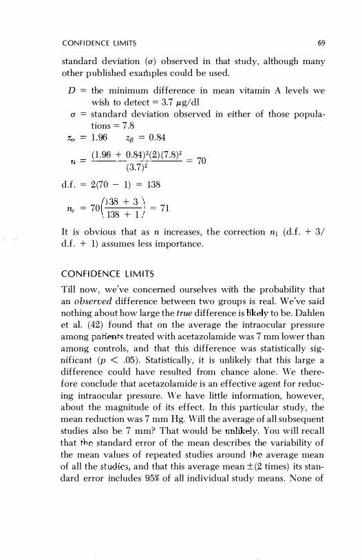
C O N F I D E N C E L I M ITS 69

standard deviation (0 ) observed in that study, although many

other published examples could be used.

D = the minimum difference in mean vitamin A levels we

wish to detect = 3.7 �g/dl

o = standard deviation observed in either of those popula­

tions = 7.8

rI

1 . 96 z{3 = 0 .84

( 1 .96 + 0 .84 ) 2 (2) (7 .8)2 = 70

(3 .7)2

dJ . =

2 (70 - 1) = 138 (138 + 3 ) ric = 70

138 + 1

= 71

It is obvious that as n increases , the correction nl (dJ. + 3/

dJ. + 1) assumes less importance .

CO N F I D E N C E L I M ITS

Till now, we've concerned ourselves with the probability that

an ohserved difference between two groups is reaL vVe've said

nothing about how large the true difference is to be. Dahlen

et a1 . (42) found that on the average the intraocular pressure

among treated with acetazolamide was 7 mm lower than

among controls , and that this difference was statistically sig­

nificant (p < .05 ) . Statistically, it is unlikely that this large a

difference could have resulted from chance alone . We there­

fore conclude that acetazolamide is an effective agent for reduc­

ing intraocular pressure . We have little information, however, about the magnitude of its effect. In this particular study, the

mean reduction 'vas 7 mm Hg. Will the average of all subsequent

studies also be 7 mm? That would be You will recall

that the standard error of the mean describes the variability of

the mean values of repeated studies around the average mean

of all the and that this average mean ± (2 times) its stan­

dard error includes 95% of all individual study means, None of

70 STAT I ST I CS

us very far, since we rarely repeat the same experi­

ment many times . To be useful, this concept must be turned on

its head : we calculate the standard error from the standard devia­

tion observed in this single experiment. The observed mean ±2 S . E . then has a 95% chance of including within it the "true" mean

for this sample. This is the 95% confidence level of our mean .

Our sample mean ±3 S . E . has a 99% chance of encompassing the

"true" mean, whatever that elusive figure is, and is therefore

the �)9% confidence interval for the mean. As we widen the inter­

val, we decrease the likelihood of missing the "true" mean, but of

course we also reduce the precision of our estimate.

Confidence intervals also have another use. If our sample was

representative of all similar individuals in the population at large

(e .g . , we had selected our ocular hypertensives randomly from

among all ocular hypertensives) , the confidence interval would

include the "true" mean for all ocular hypertensives in the

population.

Illustrative example: As an example, let us turn again to our study

of serum vitamin A levels . The mean serum vitamin A level of

randomly sampled children was 20 Mg/lOO ml. The S . E . of this mean ,yas:

S . D . 7.86 S

·E .

x = Vn = Y268 = 0 .48

The 95% confidence limits are 20 .0 ± 2( .48), or 19.0 and 21 .0 . The interval between 19 .0 and 21 .0 ,ug/IOO ml had a 95% chance

of including the true mean serum vitamin A level of 6000 children:

the population from which the 268 who contributed blood

samples had been randomly selected . The 99% confidence inter­

val would be 18 .6 to 21 .4 ,ug/IOO m!, which increases our assur­

ance but lowers our precision .

instead of the mean level, we are interested in the mean between two groups, we simply substitute the stan­

dard error of mean difference for the standard error of the

mean level. In our paired comparison between night-blind and

C O N f i D E N C E L I M ITS 71

normal children, the mean difference was 3 .77 Mg/lOO ml and the S . E . of this difference (S .D ./.J;;" = 9.0/Ji60) was 0.71 . The 95% confidence limits are therefore 2.35 and 5.19 . Similarly, in our independent (unpaired) comparison of roughly these same chil­dren, the difference between the means (xi - X2 ) was 3.7, and the standard error of the difference of the means of the two samples (Sl.2) was 0.75. The 95% confidence interval for the dif­ference between the means of the two samples is therefore 2.2 to 5 .2 . Had these been random samples of all night-blind children (and their matched controls) in Indonesia, then the "true" dif­ference between all 1 million night-blind children and matched controls in Indonesia would probably (9.5% chance) lie between these limits .

To make use of confidence limits , we need only calculate the standard error.

For measurement data, as in the above examples:

S d d standard deviation

tan ar error =

Vn the standard deviation being read off a handy pocket calculator. Calculation of the S .E . of a difference between t\yO independent samples is slightly more complex, and was already covered under tests of significance (p . 59) .

For attribute data (rates and proportions ) , the standard devia­tion and standard error are identical and calculated as follows :

S .E . (or S .D . ) = -J pqln

where

p = proportion with the attribute q = 1 - p ( the proportion without the attribute) n = size of the sample

Illustrative example: To turn again to the prevalence of punctate keratopathy among children with Bitot's spots, the observed rate was 0 .75 . Had this been a representative sample of all children

72 STATISTICS

in Indonesia with Bitot's spots (it was not ) , the true, overall p opu­

lation prevalence of SPK among them would have a 95% chance

of lying within 0.75 ± 2 S . E .

S . E .

Confidence limits 0.75 2( .055) = 0.64

0 .75 + 2( .055) = 0.86

SOM E PART I NG ADV I C E

Congratulations ! Having completed (and presumably under­

stood) this section, you now have at your disposal all the sta­

tistical tools required to carry out and evaluate the most com­

mon types of clinical studies . You can estimate sample size,

determine whether the difference between two groups (of dis­

eases, treatments, etc . ) is statistically significant, and estimate

how large that difference really is. These procedures are out­

lined in Table 26. Nonetheless, it is a good idea to consult with

Table 26 APPLICATION OF BASIC STATISTICAL PROCEDURE S

A . Tests of statistical significance 1 . Rates and proportions

(attribute data) a. Two samples

b. Three or more samples

2. Means and averages

( measurement data)

a. Paired samples

b. Two independent samples

c . Three or more samples

Normal deviate (z) Fisher's exact test (for small samples)

Chi-square (X") Chi-square (x2)

Student's t (paired analysis: D) Student's I (unpaired analysis: Xl - X2) Student's t (nonsimultaneous comparisons) Analysis of variance ( AKOVA)

(simu Itaneous comparisons)

SOM E PART I NG A DV I C E

Table 26 ( cont . )

B. Estimation of true magnitude 1. Rates and proportions

(attribute data)

2 . Means or differences (measurement data)

C. Determination of sample size 1. Rates and proportions

(attribute data)

2 . Means and averages

(measurement data)

a . Paired samples

b. Independent samples

Confidence limits

p ± (a) S . E . S . E . = Vpq/n x ± (a) S . E .

i5 ± (a ) S . E .

S . E . = S.D'/Vn a = 2, C.L. = 95% a = 3, C.L. = 99%

See text

73

an epidelniologist/statistician whenever possible, especially when

undertaking large studies utilizing many subgroups, risk factors,

end points, or sequential analyses.

Individuals involved in numerous studies will want to use

more sophisticated calculators, capable of carrying-out many of

these statistical manipulations automatically. A word of caution !

The formulations that they employ are not always adequate. For

example, the normal deviate (z) is rarely corrected for continuity,

and chi-square (for 2 X 2 tables) rarely employs the Yates correc­

tion. Before relying on any prepackaged program, be sure that

its formulation is adequate for your purposes. If not, you can

always construct your own program for use in programmable

calculators .

The statistical theory behind these various procedures , their

mathematical derivations, and additional, more complex manipu­

lations are described in detail in references S-l through

Appendix 5 .

1 . Christy, N. E . , S ommer, A. Antibiotic prophylaxis of post­

operative endophthalmitis . Ann. Ophthalmol. 1 1 : 1261-1265,

1979.

2. Hiller, R . , Kahn, A. H . Blindness from glaucoma. Am. J .

Ophthalmol. 80 :62-69, 1975.

3. Hollows, F. c. , Graham, P. A. Intraocular pressure, glau­

coma, and glaucoma suspects in a defined population. Brit.

J. Ophthalmol. 50:570-586, 1966.

4. Sommer, A . , Sugana, T. , Hussaini, G . , Emran, N . , Tarwotjo,

I . Xerophthalmia-determinants and controI. Proceed. XXIII .

Int . Congo Ophthalmol . , Shimizu, K . , Oostehuis , J . A . , eds .

Amsterdam, Excerpta Medica, 1979, pp . 1615-1618.

5. Kirk, H . 0., Petty, R . W. Malignant melanoma of the choroid:

a correlation of clinical and histological findings . Arch .

Ophthalmol . 56:843-860, 1956.

6 . Perkins, E . S. The Bedford glaucoma survey. I. Long-term

follow-up of borderline cases. Brit. J. Ophthalmol. 57: 179-

185, 1973.

7. David, R. , Livingston, D. G., Luntz, M. H. Ocular hyperten­

sion-a long-term follow-up of treated and untreated pa­

tients . Brit. J . OphthalmoL 61 : 668-674, 1977.

74

R E F E R ENCES 75

8. Indonesian Nutritional Blindness Prevention Project. Annual

Report. Bandung and �ew York: Helen Keller International,

1978.

9. Kirsch, R. E . , Anderson, D. R. Clinical recognition of glau­

comatous cupping. Am. J . Ophthalmol. 75 :442-454, 1973,

10. Sommer, A . , Pollack, I. , Maumenee, A. E. Optic disc param­

eters and onset of glaucomatous field loss . 2, Static screening

criteria. Arch. Ophthalmol. 97: 1449-1454, 1979. 1 1 . Stromberg, U. Ocular hypertension. Acta. OphthalmoL

Suppl . 69, p . 62. Copenhagen, Munksgaard, 1962.

12. Pohjanpelto, P. E. J . , PaIva, J. Ocular hypertension and glau­

comatous optic nerve damage . Acta. Ophthalmol. 52 :194-

200, 1974.

13. Bankes, J . L. K., Perkins, E . Tsolakis, S . , Wright, J . E .

Bedford glaucoma survey. Brit. Med. J . 1 :791-796, 1968 .

14. Read, J . , Goldberg, M . F. Comparison of medical treatment

for traumatic hyphema. Tr. Am, Acad. Ophthal . OtoL 78 :

799-815, 1974.

15. Peyman, G. A. , Sathar, M. L. , May, D . R. Intraocular gen­

tamycin as intraoperative prophylaxis in South India eye

camps. Brit. J. OphthalmoL 61 : 260-262, 1977.

16. The Diabetic Retinopathy Study Research Group. Photo­

coagulation treatment of proliferative diabetic retinopathy:

the second report of diabetic retinopathy study findings .

Ophthalmol. 85:82-106, 1978.

17. Kahn, H. A., Liebo\vitz, H. Ganley, J . P., Kini, M .

Colton, T . , Nicherson, R . S . , Dawber, T. R . The Framingham

eye study. II. Association of ophthalmic pathology with single

variables previously measured in the Framingham heart

study. Am. J. Epidem. 106:33-41 , 1977.

18. Van Metre, T. E ., Maumenee, A. E . Specific ocular lesions

in patients with evidence of histoplasmosis . Arch. OphthaI­

mol. 71 :314-324, 1965.

19 . Hiller, R . , Kahn, H . A. Senile cataract extraction and diabetes .

Brit, J. Ophthalmol. 60:283-286, 1976.

76 REFERENCES

20. Gasset, A. R , Houde, W. L . , Garcia-Bengochea, M . Hard contact lens wear as an environmental risk in keratoconus . Am. J . Ophthalmol. 85 :339-341, 1978.

21. Zimmerman, L. E . , McLean, 1. W., Foster, W. D. Does enu­cleation of the eye containing a malignant melanoma pre­yent or accelerate the dissemination of tumor cells? Brit . J . Ophthalmol. 62 : 420-425, 1978.

22. Jaffe, N. S . , Eichenbaum, D. M . , Clayman, H. M . , Light, D. S . A comparison of 500 Binkhorst implants with 500 routine intracapsular cataract extractions . Am. J. Ophthalmol. 85: 24-27, 1978.

23. Klein , M . L . , Fine, S . L . , Patz, A . Results of argon laser photo­coagulation in presumed ocular histoplasmosis . Am. J . Ophthalmol. 86:211-217, 1978.

24. Sommer, A . , Emran, N. Topical retinoic acid in the treatment of corneal xerophthalmia. Am. J. Ophthalmol . 86:615-617, 1978.

25. Moss, A. P., Ritch, R, Hargett, N. A . , Kohn, A. N . , Smith, H . , Podos, S. 1\1. A comparison of the effects of timolol and epinephrine on intraocular pressure . Am. J. Ophthalmol. 86:489-495, 1978.

26. Lichter, P . R . , Newman, L . P., Wheeler, N. C . , Beall, O . V.

Patient tolerance to carbonic anhydrase inhibitors . Am. J . Ophthalmol. 85:495-502, 1978.

27. Yasuna, E. i'vlanagement of traumatic hyphema. Arch. Oph­thalmol. 9 1 : 190-191 , 1974.

28. Sommer, A . , Pollack, 1 . , Maumenee, A. E . Optic disc param­eters and onset of glaucomatous field loss . 1. Methods and progressive changes in disc morphology. Arch . Ophthalmol. 97 : 1444-1448, 1979.

2R Kahn, H. A . , Leibowitz, H., Ganley, J. P . , Kini, M . , Colton, T . , Nickerson, Dawber, T. R Standardizing diagnostic procedures . Am. J. OphthalmoL 79:768-775, 1975 .

30. Edwards , W. C . , Layden, W. E . Monocular versus binocular patching in traumatic hyphema. Am. J. Ophthalmol. 76: 359-362, 1973.

R E F E R E N C E S 7 7

31 . Casscells , ·W., Taylor, S . Damned Lies. Lancet ii :687-688, 1978.

32. Weber, J . Schlagel, T. F . , Golden, B. Statistical correla-tion of uveitis syndromes with virus titers . Am. J. Ophthalmol. 78 :948-951 , 1974.

33. Blegvad, O. Xerophthalmia, keratomalacia and xerosis con­junctivae. Am. J. Ophthalmol. 7 :89-1 17, 1924.

34. Sommer, A . Cataracts as an epidemiologic problem. Am. J . Ophthalmol. 83:334-339, 1977.

35, Sommer, Hussaini, G . , Muhilal, Tarwotjo, Susanto, D . , Sarosa, S . -Iistory of nightblindness : a simple tool for xero­phthalmia screening. Am. J. Clin . Nutr. (in press) .

36 . The Diabetic Retinopathy Study Research Group . Prelimi­nary report on effects of photocoagulation therapy. Am. J . Ophthalmol. 81 :383-396, 1976.

37. Sommer, A. Toward a better understanding of medical re­ports . Am. J . Ophthalmol. 79 :1053- 1056, 1975.

38. Sommer, A. Keratoconus in contact lens wear . Am. J. Oph­thalmol. 86:442-443, 1978.

39. Ederer, F . , Ferris, F. Studying the role of an environmental factor in disease etiology. Am. J. Ophthalmol . 87:434-435, 1979.

40. Sommer, A . , Emran, N. , Tamba, T. Vitamin A responsive punctate keratopathy in xerophthalmia. Am. J. Ophthalmol. 87 :330-333, 1979.

41 . Diamond, E. Temple, B. Tables of the power of the COll-

ditional test for equality of two Poisson parameters . Dept. of Epidem. , Johns Hopkins University School of Public Health .

42. Dahlen, L . , Epstein , D . Grant, W. M . , Hutchinson, B . T . , Prien , E . L. , Krall , J . M. A repeated dose-response study of methazolamide in glaucoma. Arch . Ophthalmol. 96:2214-

1978.

AP PI= N D I X 1

TA B L E O F RAN DOM N UM B ERS

1 2 :3 4 5

6 7 8 9

10

1 1 1 2 1 3 1 4 1 5

1 6 17 18 [9 20

21 22 23 24 25

26 27 28 29 30

31 32 J3 34

3:\

36 37 38 39 40

2 3 4

o 6 2 8 ,3 4 2 5 :3 4 7 4 4 7 5 0 9 3 6

8 6 1 5 2 2 2 ,1

2 3 3 4 2 0 4 2 6 ,5 3 :3

3 9 2 9 7 2 2 J

7 4 0 7 9 7 2 2

9 9 8

7 2 9 4 9 1 5 2 6 9 3 4 (i 2 6 o 7 4

3 7 r,

4 B 3 0 4 1 2

7 5 6 7 4 0 6

2 1 4 1 7 0 0 2 4 6 4 7 6 2 9 2 9 0

3 7 9 8 9 6 5 0 2 2 9 3 5 8 9 9

9 8 0

6 6 9 3 3 1 7 4 9 B 0 :3 9 9 7 3 6 .3 8 2

.5 6 7 8

3 5 7 6 2 (J 3 0 1 5 8 8 4 8 3 ,3

8 J 7

7 5 3 7 2 7 1 2 7 5 8 2 6 0 5 7

o 3

8 9 S 4 8 4 5 9 3 7 4 2 8 0 3 9 9 3 1) 4

6 1 6 7 3 0 2 6 5 2 8 0 5 6 2 9 1 6 0 6

7 2 6 0 8 5 6 9 o 3 :3 6 9 4 1 6 5 5 8 4

o 4 6 1 6 9 0 1 2 4 6 8 0 3 9 8 6 7 4

o 9 7 5 1 0 6 J 0 5 9 7 1 0 6 6 5 2

9 0 9 3 7 0 0 5 4 9 1 2 J 0 3 3 o 7 2 6

9 10 1 1 12

4 9 5 1 9 9 o 5 2 0

6 6 4 4 o 2 9 4 (} 9

4 6 5 6 6 8 9 8 4 2

9 R

5 13

6 2 5 :3 2

2 7 5 9 7 0 o 8 6 7

2 0 3 7 9 6 5 0 5 2

9 1 9 7 1 5 7 9 4

3 5 9 6 4 0 8 8 J 6

o 7 5 1 4 0 7 4 7 8

4 9 3 8 8 5 o 2

4 6 5 9 6 5 1 5 2 1

7 5 2

4 7 2 7 8 2

7 2 4 9 1 4 9 2 3 6

8 ,5

4 5 9 1

4 9 5

:] 8 5

& 4 6 9 o 7

6 6 9 4 7 2 2 4 3

13 14 15 16

6 6 3 ,5

3 4 8 4 3 5

5 0 2 6 4 4 4 6 7 3

8 6 2 5 .3 1

4 4 6

3 7 2 3 9 2 4 1 7 8

5 6 7 5 -1 1 6 0 5 2

2 2 9 5 1 1 8 6 6 2

7 7 4 7 4 9 4 3 1 0

9 0 5 3 6 9

3

8 0 7 1 3 6 :; 9 8 6

1 5 0 1 8 o :3

7

3 :3 3 2 8 9 7 9 5 7

4 6 7 9 9 6 o 8 3 7

8 3 4 3 5 1 7 0 6 5

7 9 4 7 9 2 3

5

3 8 9

7 6 4 6 1 6

3 0 o 2 6 4 6 1 8

Reproduction of Table I of A. Bradford Hill: Principles of Medical Statistics, London,

Lancet, by permission of the author and publisher.s.

78

TAB L E OF RAN DOM N U M B ERS

1 2 3 4 5 6 7 8 9

10 1 1 1 2 1 :3 1 4 1 5 1 6 1 7 l b 1 9 20 2 1 22 23 24 25 26 27 2R 29 30 :11 :32 31 34 35

36 37 38 .39 40

2 3' 4

2 8 6 9 4 0 4 0 1 6 0 2 8 4 3 8 5 7 5 4 4 3 4 3 7 2 3 7 0 0 9 9 7 6 5 3 2 5 9 9 8 3 6

8 9 2 1 2 6 9 5 1 4 o 5 1 0 2 8 8 4 6 5 6 3 8 8 8 0 :3 9 3 4 4 6 4 7 4 0 1 8 7 5 8 0 3 6 4 4 7 0 2 9 1 9 0 :3 4 2 9 1 5 9 o 9 6

6 2 .5 \) 3 6 o 9 0 2

,5 0 3 6 ·1 0 4 3 8 4 4 .5 1 3 1 2 3 1 4 1 9 3 3 3 9 1 8 4 8 8 8 3 5

5 6 7 8

3 0 9 6 5 8 7 ,3 7 7 3 1 1 8 5 0 3 7 7 0 f! 5 0 2 o 4 6 0 S 0 4 6 0 9 7 9 3 9 o 3 8 9 o 3 2 1 9 8 3 7 5 6 4 5 5 2 9 5 9 7 8 2 6 0 5 1 6 9 6 5 3 3 6 G 7 I I

7 .5 {) 1 8 2 6 fi " 2 5 2 1 8 8 6 2 0 5 9 ,1 .5 4 6 8 6 8 5 3 7 o :3 6 o 5 4 9 7 8 9 9 5 8 7 2 7 3 6 4 5 2 4 9 7 6 9 9 6 2 2

" 5 fj 0 5 (i :3 8 6 9

9 10 1 1 12

6 3 9 4 o 4 5 6 3 2 6 6 3 0 9 2 4 4 8 3 -: 4 1 4 o

4 7 4 o () 1 k 5 0 4 4 8 5 7 9 9 9 4 .5 6 2 4 5 3 1 9 6 4 8 o 4 7 3 5 0 4 0 I 4 6 4 5 :3 4 3 o 6

9 2 3 7 9 9 3 7 4 9 2 5 7 3 6 6 7 0 6 5 0 6 8 fi 1 () :1

7 3

-1 9 6 8 9 fj 5 I

6 6 :3 (J :1 9 8 5 o 3 1 5 2 0 5 9 (J 0 9

:3 2 7 8 2 5 7 6 8 7 3 2 0 7 8 () :3

13 14 15 16

9 6 7 6 4 4 7

() 8 6 4 0 6 9 8 0 8 4 9 2 6 9 8 2 7 7 8 3 7 6 6 6 3 5 0 o 0 4 4 6 2 o 8 7 5 5 4 7 2 1 8 4 -; 1 9 1 2 8 7 1 2 2 9 4 6 (-) ;) 1 3 6 7 2 2 4 7

6 5 6 4 7 9 2 �j

'j

8 0 1 8 1 9 5 8 o 4 4 2 9 8 o 6 4 3 2 4 9 7 0 3 3 1 8 5 9 4 2 3 7 8 9 3 5 4 1

7 2 7 6 o 8 8 7 8 5 o 7 4 5 7 4

5 2 9 1 2 2 6 6 3 7 7 4 5

Reproduction of Table II of A. Bradford Hill: Principles of Medical Sta!i.I,'tic,\, Londoll,

Lancet, by permission of the author and publishers.

79

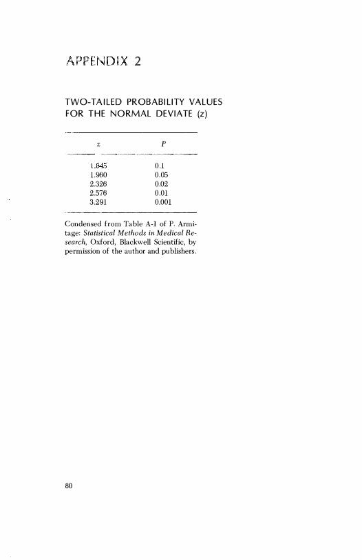
j 'PE N D I - 2

TWO-TA I L E D PROBAB I L I TY VA L U E S

F O R T H E N O RMAL D E V I ATE (z )

z P

1 .645 0.1 1 .960 0.05 2.326 0.02 2.576 0.01 3.291 0.001

Condensed from Table A-I of P. Armi­tage: Statistical Methods in Medical Re­search, Oxford, Blackwell Scientific, by permission of the author and publishers .

80

ENDIX 3

PRO BA B I L I TY VAL U ES F O R CH I -SQ U A R E (Xl)

Probability Degrces of

freedom 0.10 0 .05 0.01 0.001

1 2 .706 3.841 6 .6,35 10.827 2 4 .605 5.991 9.210 13.815 :) 6.251 7.815 1 1 .345 16.268 4 7.779 9 .488 ' 13.277 18.465 5 9 .236 1 1 . 070 15.086 20.517

6 10.645 12.,592 16.812 22 .457 7 12.017 14.067 18.475 24 .322 8 13.362 15.507 20.090 26. 125 9 14.684 16.919 21 .666 27.877

10 15.987 18.307 23.209 29.588

1 1 17.275 19.67.5 24.72.5 :31.264 12 18.549 21 .02G 26.217 32.909 13 19.812 22.362 27.688 ,34.528 14 21 .064 23.685 29. 141 36.12:3 15 22.307 24.996 30.578 37.697

16 23.542 26.296 32.000 39.252 17 24.769 27 .587 33.409 40 .790 18 2.5.989 28 .869 34 .805 42.312 19 27.204 30. 144 36.191 4:3.820 20 28.412 31 .410 37.566 4.5.:315

Adapted from Table IV of R. A . Fisher and F. Yates: Statistical Tables for Biolog-ical, Agricultural and Medical Research, London, Longmans Group, by permis-sion of the authors and publisher.

81

A P P E N D I X 4

TWO-TA I LED PROBAB I L I TY VAL U ES FOR STU D E N T'S t TEST

Probability Degrees of fJ'eedom 0.10 0.05 0.01 0.001

1 6.314 12.706 63.657 636.619 2 2.920 4.303 9.925 31.598 3 2.353 3. 182 5.841 12.941 4 2. 132 2.776 4 .604 8.610 5 2.015 2.571 4.032 6.859

6 1 .943 2.447 3.707 5.959 7 1 .895 2.365 3.499 5.405 8 1 .860 2.306 3 . . '355 5.041 9 1 .833 2.262 3.250 4.781

10 1 .812 2 .228 3. 169 4.587

1 1 1 .796 2.201 3. 106 4.437 12 l .e782 2. 179 3.055 4.318 13 1 .771 2. 160 3.012 4.221 14 1 .761 2. 145 2.977 4. 140 15 1 .753 2.131 2.947 4.073

16 1 .746 2 .120 2.921 4.015 17 1 .740 2 . 110 2.898 3.965 18 1 .734 2 . 101 2.878 3.922 19 1 .729 2.093 2.861 3.883 20 1 .725 2.086 2.845 3.850

21 1 .721 2.080 2.831 3.819 22 1 .717 2.074 2.819 3.792 23 1 .714 2.069 2.807 3.767 24 1 .711 2.064 2.797 3.745 25 1 .708 2.060 2.787 3.725

26 1 .706 2.056 2.779 3.707 27 1 .703 2.052 2.771 3.690 28 1 .701 2.048 2.763 3.674 29 1 .699 2.045 2.756 3.659 30 1 .697 2.042 2.750 3.646

00 1 .64.5 1 .960 2.576 3.291

Adapted from Table III of R. A. Fisher and F . Yates: Statistical Tables for Biological, Agricultural and Medical Research, London, Longmans Group, by permission 01 the authors and publisher.

82

AF 5

BACKGRO U N D A N D SOU RC E MATE R I A L

Ep idem io logy

E-1 . Lilienfeld, A. M. Foundations of Epidemiology. New York :

Oxford University Press, 1976.

E-2. Lilienfeld, A . M . , Pederson, E . , J . E . Cancer Epi-

Methods of Study. Baltimore: Hopkins

Press, 1967.

E-3. Pugh, T. F. Epidemiology, and

Methods. Boston: Little , Brown, 1970.

E-4 . Fox, J . P . , Hall, C. E . , Elverback, L. R. Epidemiology: Man

and Disease. New York: Macmillan, 1970 .

E-5. Slonim, M . J . Sampling. New York: Simon & Schuster, 1960.

Stat i st i cs

S-1 . Armitage, P. Statistical Methods in Medical Research. Ox-

ford: B lackwell Scientific Publications, 1971 .

S-2. Swinscow, T . D . V . Statistics a t Square One . London: British

Association, 1976 .

S-3. J . L . Statistical Methods for Rates and Proportions.

New York: John Wiley & Sons, 1973.

S -4 . Snedecor, G. W., Cochran, W. C. Statistical Methods. Ames :

Iowa S tate Press, 1967.

8-5 . Neter, J . , Wasserman, W. Applied Linear Statistical Models.

Homewood, Ill . : Richard D. Irwin, 1974.

8-6 . Hill, A . B . A Short Textbook of Medical Statistics. Phila­delphia: Lippincott, 1977 .

83

In ex

Adjustment, rate, 28-29

Alpha error, 48-49, 64-65

Analysis of variance, 63

Associations, statistical, 21, 39

alternative explanations for, 39-41

Attack rate, 3, 4

group specific, 6, 7

Attribute data, 49

methods for determining: sample size, 65-67; standard deviation, 71 ; standard error, 71; statistical significance, 49-56. See also

Normal deviate; Chi square

Beta error, 65

Bias, 24

as cause of spurious association, 40

observer, 34, 35

patient, 33

sampling (selection) , 24-27, 29

due to loss to follow-up, 29, 30

Blindness

84

glaucoma, 4, 5; relative risk, 6;

whites vs. nonwhites, 5, 7, 8

Model Reporting Areas, 4

Calculators, use of, 58, 73

Case-control study. See Retrospective

study Cataracts, diabetes, 21 -23, 25, 41

Chance (variation) , 37, 38, 48-50, 61 , 65

Chi square (X2 ) , 52-56

table, probability values for, 81

Clinical studies, organization, 45

critical steps , summary, 45-46

Confidence limits ( interval) , 69-72

Contact lenses, sampling bias in keratoconus, 25

Contingency tables, 53-56

Controls, 25, 30, 31

concurrent, 32, 33

nonconcurrent, 31, 32

use of matching, 30, 31

Correction for continuity, 51, 56, 73

Crossover study, 31 , 33

Cupl disc ratio, observer variation, 34, 35

Degrees of freedom, 55, 59-61, 68

Diabetic retinopathy

associations, 40

prospective study, 18, 19

II\IDEX

Endophthalmitis, postoperative attack rate, 3 , 4, 6, 31-33 prophylaxis, 3, 5, 18, 31-33 relative risk, 5, 19

Epidemiology, characteristics, 3 Error

alpha, 48, 49, 64, 65 beta, 65

False negatives and positives, 14-16 Fisher's exact test, 52 Framingham study, 19, 20

Glaucoma blindness, registry data, 4, 5, 42;

group specific rates, 5, 7, 8; relative risk, 6

field loss, incidence, 9, 14 screening, tonometry, 12, 13, 15, 16

Histoplasmosis, ocular, 21, 30

Incidence definition, 7, 9 in prospective study, 18, 19 relation to prevalence, 9 , 10 uses, 10, 11

Independent ( grouped) samples, 31, 58, 60, 62. See also Measurement data

Inferences, epidemiologic, 7, 41-43 Intraocular

lens, 26, 27 pressure, 57, 63, 69

Longitudinal study. See Prospective study

Loss to follow-up as cause of sampling bias, 29 methods for handling/minimizing,

29, 30

Malignant melanoma enucleation and mortality, 25, 26 incidence, prevalence, 10 intraocular, unrecognized, 8 p32 testing, false positive/ nega tive,

15

Masking, 33, 34 Matching, 25-29

of controls, 30, 31 Mean, 57-59

difference, 61 , See also Standard error of the

'�ean Measurement data, 56

sample size, determination of, for independent samples, 59, 68; for paired samples, 67, 68

standard deviation, calculation of, for independent samples, 58; for paired samples , 61

85

standard error, �alculation of, 71 tests of significance, for independent

samples, 58,161; for paired samples, 61-62; for three or more samples, 62, 63. See also Student's t test

Mortality rate, affect on prevalence, 10 Murphy's law, 44

Normal deviate (z) , 49-53, 56, 59 correction for continuity in, 51 table, probability values for, 80

One-tailed distribution, 65

Paired comparisons, value of, 31 , 61 , 62 . See also Measurement data

Placebo, 33 Prevalence

definition, 7, 8 relation to incidence, 9, 10 uses, 10, 11

ProspectiYc study, 16-18, 20 concurrent/nonconcurrent, 19, 20, 26 controls, use of, 31 , 32 incidence in, 18 loss to follow-up, affect on, 29 , 30 randomization, use of, 26 relative risk, calculation of, 19 sampling bias in, 25, 26, 29

Random numbers, table of, 78, 79 RandOrrllzation, 26, 27

matching in, 28

86

technique, 28 to minimize bias, 40

Rates, meaning and use, 3 adjustment of, 28, 29 attack, 3, 4, 6, 7 false positive/negative, 14-16 group specific, 6-8, 29 incidence, 7, 9-1 1 , IS, 19 prevalence, 7-11 sensitivity, 11-15 specificity, 11-15 types of, summary, 43

Relative risk, 5, 6 combined prophylaxis, endophthal­

mitis, 5 glaucoma blindness; race, age, sex,

6, 7 incidence as basis, 1 1 i n prospective study, 1 9 i n retrospective study, 23

Reproducibility, 35, 36 Retrospective study, 16, 17, 21, 22

relative risk, calculation of, 23 sampling bias in, 25

Risk factors, 7, 20

S ample size, 38, 50 calculation of, 64; for attribute data,

65-67; for measurement data: independent samples, 68; paired samples, 67, 68

determination, importance of, 36, 37, 63, 64

Screening, 12-16, 42 Senile macular degeneration, 27 Sensitivity, 1 1-15 Significance

clinical, interpretation, 38, 63, 64 statistical, interpretation, 37, 38, 47,

48, 50, 63, 64; test of: for attribute data, 49-54; for measurement data, 58-63. See also Normal deviate ( z ) ; Chi square (x2 ) ; Student's t

Specificity, 11-15 Standard deviation, 57, 58, 61

calculation of: for attribute data,

INDEX

71; for independent samples, 58; for paired differences, 61

Standard error of the mean, 57-59 calculation of, 58; for attribute data,

71; for difference between independent samples, 59; for mean difference in paired samples, 61

use in establishing confidence limits, 69, 70

Standardization, 28, 29 Statistical procedures, summary, 72, 73 Statistical tests. See Significance,

statistical Student's t

calculation of, for difference be­tween independent samples, 59, 62, 63; for mean difference between paired samples, 61

table, probability values for, 82

Test of significance. See Attribute data; Measurement data

Tonometry, glaucoma screening, 12-14 Traumatic hyphema, 18, 31, 37 Two-tailed distribution, 50

table, normal deviate, 80

Variability interobserver, 34-36 intraobserver, 34 methods for minimizing, 35

Vitamin A deficiency Bitot's spot, prevalence, incidence,

10 corneal disease, prevalence of

malnutrition, 8

Xerophthalmia corneal destruction, incidence,

prevalence, 10 epidemic, 40 night blindness, 42 punctate keratopathy, 50, 51, 53, 54 serum vitamin A comparison, 60,

62, 70

Yate's correction, 56, 73