Embed Size (px)
Citation preview
Algorithm Theoretical Basis Document
Issue: 1
Date of issue: 7/05/2020
Reference: Ozone_cci+_D2p1_ATBD_1
Page 1-42
Ozone_cci+
Algorithm Theoretical Basis Document (ATBD)
Date: 07/05/2020
Version: 1
WP Manager: R. Siddans
WP Manager Organization: STFC Rutherford Appleton Laboratory
Other partners: DLR-IMF, KNMI, RAL, ULB, UBR, FMI

Algorithm Theoretical Basis Document
Issue: 1
Date of issue: 7/05/2020
Reference: Ozone_cci+_D2p1_ATBD_1
Page 2-42
DOCUMENT PROPERTIES
Title Algorithm Theoretical Basis Document (ATBD)
Reference Ozone_cci+_D2p1_ATBD_1
Issue 1
Revision 0
Status Draft
Date of issue 7 May 2020
Document type D2.1
FUNCTION NAME DATE SIGNATURE
LEAD AUTHOR
Project Parnter Richard Siddans
CONTRIBUTING
AUTHORS Project partner
M. Coldeway-Egbers , C.
Lerot, V. Sofieva, R. van der
A, C. Wespes
REVIEWED BY
Project partner
ISSUED BY Science Leader Richard Siddans

Algorithm Theoretical Basis Document
Issue: 1
Date of issue: 7/05/2020
Reference: Ozone_cci+_D2p1_ATBD_1
Page 3-42
DOCUMENT CHANGE RECORD
Issue Revision Date Modified items Observations
0 0 14/02/2020 Initial template Creation of document

Algorithm Theoretical Basis Document
Issue: 1
Date of issue: 7/05/2020
Reference: Ozone_cci+_D2p1_ATBD_1
Page 4-42
Executive Summary
The Algorithm Theoretical Basis Document (ATBD, deliverable D2.1 in Ozone_cci+) describes
the algorithms used for total ozone columns, nadir-based ozone profiles, and limb-based ozone
profiles.
A series of new algorithms will be developed with a focus on both level-2 and level-3 data
products.
For total ozone, the following activities will be undertaken:
- Integration of Sentinel-5P and MetOp-C/GOME-2 in the GTO-ECV data record, based on
the reference GODFIT level-2 algorithm
- Merging of GTO-ECV data record with historical NASA/SBUV/TOMS data records to
create a 40-year CDR starting in 1979
- Tentative expansion of the MSR data record back to 1960 using ground-based total ozone
measurements
For ozone profiles from nadir sensors:
- Integration of Sentinel-5P and MetOp-C/GOME-2 in CCI data sets based on the reference
RAL level-2 retrieval algorithm
- Creation of a first European merged ozone profile and total ozone data record (GOP-ECV)
starting with ERS-2/GOME in 1995 and consistent with the GTO-ECV total ozone data
record
- Improvement of IASI level-2 retrieval algorithm (FORLI) to reduce uncertainties and
systematic biases in the UTLS region
- Exploration of the potential to reduce uncertainties in nadir profile level-2 products in the
lower troposphere and UTLS through exploitation of the synergy between UV, VIS and
TIR retrievals
For ozone profiles from limb sensors:
- Integration of several new sensors (POAM-III on SPOT-4, SAGE-III on Meteor-3M, and
SAGE-III on ISS) in the HARMOZ data record
- Intercomparison of different competing OMPS-LP level-2 retrieval algorithms. This
activity might lead to the identification of a need for a dedicated round-robin exercise.
- Improvement of OMPS-LP level-2 algorithm in the UTLS and in polar regions
- Extension of the merged SAGE-II/CCI/OMPS long-term zonal mean data record with
additional sensors to improve its accuracy, especially in lower stratosphere
- Improvement of latitude-longitude gridded level-3 data products based on limb-type
sensors

Algorithm Theoretical Basis Document
Issue: 1
Date of issue: 7/05/2020
Reference: Ozone_cci+_D2p1_ATBD_1
Page 5-42
Table of Contents
1 Purpose and scope ................................................................................................................... 7 1.1 Purpose ........................................................................................................................... 7
1.2 Scope ................................................................................................................................. 7 1.3 Applicable documents ...................................................................................................... 7 1.4 References documents ...................................................................................................... 7
1.5 Acronyms ....................................................................................................................... 11 2 Total Ozone ECV Retrieval Algorithms ............................................................................... 13
2.1 GODFIT (BIRA) ............................................................................................................ 13 2.1.1 Total ozone retrievals from TROPOMI/S5P ......................................................... 14
2.1.2 Total ozone retrievals from GOME-2/Metop-C .................................................... 16 2.2 GOME-type Total Ozone - Essential Climate Variable (GTO-ECV) (DLR) ................ 18
2.2.1 Total ozone L3 algorithm ...................................................................................... 18 2.2.2 The individual level-2 total ozone observations as described in Sect. 2.1 are
converted into a level-3 product, i.e. they are mapped onto a regular global grid of 1°x1° in
latitude and longitude to construct daily averages for each sensor. Each grid cell contains an
average of all level-2 data from the same day, whose center coordinates fall in the respective
grid cell. Total ozone merging algorithm ............................................................................. 18 2.2.3 GTO-ECV extension backward in time ................................................................ 18
2.3 Multi-Sensor-Reanalysis scheme (KNMI) ..................................................................... 20 2.3.1 Introduction MSR algorithm ................................................................................. 20
2.3.2 Algorithm update to extend the MSR data set into the past .................................. 22 3 Nadir Profile ECV Retrieval Algorithms .............................................................................. 24
3.1 RAL nadir profile ECV retrieval algorithms (RAL) ...................................................... 24
3.2 IASI FORLI Ozone profile retrieval algorithm (ULB) .................................................. 25
3.2.1 Basic retrieval equations ....................................................................................... 25 3.2.2 Assumptions, grid and sequence of operations ..................................................... 25
Spectral ranges ....................................................................................................... 25 Vertical grid ........................................................................................................... 25 Ozone state vector .................................................................................................. 25
Other state vector elements .................................................................................... 26
Measurement covariance matrix ............................................................................ 26
3.2.3 Iterations and convergence .................................................................................... 27 3.2.4 Forward model ...................................................................................................... 27
Atmospheric state input to the RTM ................................................................. 27 L1C radiances .............................................................................................. 27 Temperature and humidity profiles .............................................................. 27
Surface temperature ..................................................................................... 27 Cloud fraction .............................................................................................. 27 CO2 profile ................................................................................................... 27
Algorithm Theoretical Basis Document
Issue: 1
Date of issue: 7/05/2020
Reference: Ozone_cci+_D2p1_ATBD_1
Page 6-42
Orography .................................................................................................... 27 Emissivity..................................................................................................... 27
Lookup-tables............................................................................................... 28 Spectroscopy ................................................................................................ 28
Radiative Transfer Model (RTM) ...................................................................... 28 3.2.5 Error description .................................................................................................... 28 3.2.6 Output product description .................................................................................... 28
Formats .................................................................................................................. 28 Ozone profile and characterization ........................................................................ 29
3.2.7 Retrievals and Quality flags .................................................................................. 29
3.3 Combined uv/vis/thermal-ir retrieval algorithm (RAL) ................................................. 30 3.3.1 Overview ............................................................................................................... 30 3.3.2 Chappuis retrieval scheme..................................................................................... 30
3.3.3 RAL Infra-red / Microwave sounder retrievals ..................................................... 31 3.3.4 L2-L2 Combination ............................................................................................... 31
4 Limb profile ECV Retrieval / Merging Algorithm ............................................................... 35
4.1 HARMonized dataset of OZone profiles (HARMOZ) (Bremen) ................................... 35 4.2 OMPS Retrieval Schemes (Bremen) .............................................................................. 37
4.2.1 OMPS-LP NASA retrieval algorithm version 2.5 ................................................ 37 4.2.2 OMPS-LP IUP retrieval algorithm version 2 ........................................................ 37 4.2.3 OMPS-LP Usask retrieval algorithm .................................................................... 39
4.3 SAGE-CCI-OMPS Extension (FMI) .............................................................................. 39
4.4 Gridded merged Level 3 dataset (FMI) .......................................................................... 42
Algorithm Theoretical Basis Document
Issue: 1
Date of issue: 7/05/2020
Reference: Ozone_cci+_D2p1_ATBD_1
Page 7-42
1 Purpose and scope
1.1 Purpose
This document describes the algorithms used in the Ozone_cci+, addressing total ozone columns,
nadir-based ozone profiles, and limb-based ozone profiles.
1.2 Scope The scope of the ATBD is to document algorithms used in the CCI+ project, with particular
emphasis on algorithm features which are new in CCI+. Where algorithms are already described
by existing ATBDs or similar documents, references are made to these documents and only a brief
overview of the algorithmic basis is given.
1.3 Applicable documents
[AD-1] Data Standards Requirements for CCI Data Producers. Latest version at time of
writing is v1.2: ref. CCI-PRGM-EOPS-TN-13-0009, 9 March 2015, available online
at: http://cci.esa.int/sites/default/files/CCI_Data_Requirements_Iss1.2_Mar2015.pdf
[AD-2] CCI Data Policy v1.1. Available online at:
https://earth.esa.int/documents/10174/1754357/RD-7_CCI_Data_Policy_v1.1.pdf
1.4 References documents
[RD-1] GCOS Climate Monitoring Principles, November 1999, reproduced in [RD-5], p48.
[RD-2] Guideline for the Generation of Satellite-based Datasets and Products meeting GCOS
Requirements, GCOS Secretariat, GCOS-128, March 2009 (WMO/TD No. 1488).
Available online at: http://library.wmo.int
[RD-3] Quality assurance framework for earth observation (QA4EO): http://qa4eo.org
[RD-4] EU Research Programmes on Space and Climate: Horizon 2020 (H2020),
(http://ec.europa.eu/programmes/horizon2020/en/h2020-section/space,
https://ec.europa.eu/programmes/horizon2020/en/h2020-section/climate-action-
environment-resource-efficiency-and-raw-materials) and Copernicus
(http://www.copernicus.eu/).
[RD-5] The Global Observing System for Climate: Implementation Needs, GCOS-200,
October 2016. Available online at: http://library.wmo.int
[RD-6] Status of the Global Observing System for Climate, GCOS-195, October 2015.
Available online at: http://library.wmo.int

Algorithm Theoretical Basis Document
Issue: 1
Date of issue: 7/05/2020
Reference: Ozone_cci+_D2p1_ATBD_1
Page 8-42
[RD-7] Joint Committee for Guides in Metrology, 2008, Evaluation of measurement data —
Guide to the expression of uncertainty in measurement (GUM), JGCM 100: 2008.
Available online at http://www.bipm.org/en/publications/guides/gum.html.
[RD-8] Copernicus Space Component:
www.esa.int/Our_Activities/Observing_the_Earth/Copernicus/Space_Component
[RD-9] User requirements for monitoring the evolution of stratospheric ozone at high vertical
resolution (Operoz), 2015, ESA Expro contract 4000112948/14/NL/JK. Available
online at:
http://projects.knmi.nl/capacity/Operoz/Operoz_final_report_with_exec_summary_1m
ar2015.pdf
[RD-10] Boynard, A., et al.: Validation of the IASI FORLI/EUMETSAT O3 products using
satellite (GOME-2), ground-based (Brewer-Dobson, SAOZ, FTIR) and ozonesonde
measurements, Atmos. Meas. Tech.,https://doi.org/10.5194/amt-11-5125-2018 , 2018.
[RD-11] Cariolle, D. and Teyssèdre, H.: A revised linear ozone photochemistry parametrization
for use in transport and general circulation models: Multi-annual simulations, Atmos.
Chem. Phys. Discuss., 7, 1655–1697, 2007.
[RD-12] Chance, K., Burrows, J et al., Satellite measurements of atmospheric ozone profiles,
including tropospheric ozone, from ultraviolet/visible measurements in the nadir
geometry: a potential method to retrieve tropospheric ozone, J. Quant. Spectrosc. Radiat.
Transfer Vol. 51. No. 4, pp. 461476, 1997
[RD-13] Chinaud, J., et al.: IASI-C L1 Cal/Val System performance synthesis. EUMETSAT
Technical Note IA-NT-0000-4477-CNES,
https://www.EUMETSAT.int/website/home/News/DAT_4439637.html, 2019.
[RD-14] Coldewey-Egbers, M., Loyola, D. G., Koukouli, M., Balis, D., Lambert, J.-C.,
Verhoelst, T., Granville, J., van Roozendael, M., Lerot, C., Spurr, R., Frith, S. M., and
Zehner, C.: The GOME-type Total Ozone Essential Climate Variable (GTO-ECV) data
record from the ESA Climate Change Initiative, Atmos. Meas. Tech., 8, 3923–3940,
https://doi.org/10.5194/amt-8-3923-2015, 2015.
[RD-15] Coldewey-Egbers, M., Loyola, D., Labow, G., and Frith, S.: Comparison of GTO-ECV
and Adjusted-MERRA total ozone columns from the last two decades and assessment
of interannual variability, Atmos. Meas. Tech. Discuss., https://doi.org/10.5194/amt-
2019-297, in review, 2019.
[RD-16] Eskes, H. J., van Velthoven, P. F. J., Valks, P. J. M. and Kelder, H. M.: Assimilation of
GOME total ozone satellite observations in a three-dimensional tracer transport model,
Q. J. R. Meteorol. Soc., 129, 1663-1681, 2003.
[RD-17] Garane, K., Lerot, C., Coldewey-Egbers, M., Verhoelst, T., Koukouli, M.E., Zyrichidou,
I., Balis, D.S., Danckaert, T., Goutail, F., Granville, J., Hubert, D., Keppens, A.,
Lambert, J.-C., Loyola, D., Pommereau, J.-P., Van Roozendael, M., and Zehner, C.:

Algorithm Theoretical Basis Document
Issue: 1
Date of issue: 7/05/2020
Reference: Ozone_cci+_D2p1_ATBD_1
Page 9-42
Quality assessment of the Ozone_cci Climate Research Data Package (release 2017) –
Part 1: Ground-based validation of total ozone column data products, Atmos. Meas.
Tech., 11, 1385-1402, doi:10.5194/amt-11-1385-2018, 2018.
[RD-18] Garane, K., Koukouli, M.-E., Verhoelst, T., Lerot, C., Heue, K.-P., Fioletov, V., Balis,
D., Bais, A., Bazureau, A., Dehn, A., Goutail, F., Granville, J., Griffin, D., Hubert, D.,
Keppens, A., Lambert, J.-C., Loyola, D., McLinden, C., Pazmino, A., Pommereau, J.-
P., Redondas, A., Romahn, F., Valks, P., Van Roozendael, M., Xu, J., Zehner, C.,
Zerefos, C., and Zimmer, W.: TROPOMI/S5P total ozone column data: global ground-
based validation and consistency with other satellite missions, Atmos. Meas. Tech., 12,
5263–5287, https://doi.org/10.5194/amt-12-5263-2019, 2019.
[RD-19] Hollmann, R., et al., The ESA climate change initiative: Satellite data records for
essential climate variables. American Meteorological Society. Bulletin, Vol. 94, No.
10, 2013, p. 1541-1552.
[RD-20] Hurtmans, D,. et al.: FORLI radiative transfer and retrieval code for IASI, Journal of
Quantitative Spectroscopy and Radiative Transfer,
https://doi.org/10.1016/j.jqsrt.2012.02.03, 2012.
[RD-21] Keppens, A., J.-C. Lambert, J. Granville, D. Hubert, T. Verhoelst, S. Compernolle, B.
Latter, B. Kerridge, R. Siddans, A. Boynard, J. Hadji-Lazaro, C. Clerbaux, C. Wespes,
D. R. Hurtmans, P. F. Coheur, J. van Peet, R. van der A, K. Garane, M. E. Koukouli, D.
S. Balis, A. Delcloo, R. Kivi, R. Stübi, S. Godin-Beekmann, M. Van Roozendael, C.
Zehner: Quality assessment of the Ozone_cci Climate Research Data Package (release
2017): 2. Ground-based validation of nadir ozone profile data products, Atmos. Meas.
Tech., 11, 3769–3800,https://doi.org/10.5194/amt-11-3769-2018, 2018.
[RD-22] Kerr, J. B.: New methodology for deriving total ozone and other atmospheric variables
from Brewer spectrophotometer direct sun spectra, J. Geophys. Res., 107(D23), 4731,
doi:10.1029/2001JD001227, 2002.
[RD-23] Koukouli, M. E., Lerot, C., Granville, J., Goutail, F., Lambert, J.-C., Pommereau, J.-P.,
Balis, D., Zyrichidou, I., Van Roozendael, M., Coldewey-Egbers, M., Loyola, D.,
Labow, G., Frith, S., Spurr, R. and Zehner, C.: Evaluating a new homogeneous total
ozone climate data record from OME/ERS-2, SCIAMACHY/Envisat, and GOME-
2/Metop-A, J. Geophys. Res. Atmos., 120(23), 12,296-2,312,
doi:10.1002/2015JD023699, 2015.
[RD-24] Krol, M., S. Houweling, B. Bregman, M. van den Broek, A. Segers, P. van Velthoven,
W. Peters, F. Dentener and P. Bergamaschi: The two-way nested global chemistry-
transport zoom model TM5: algorithm and applications, Atmos. Chem. Phys., 5, 417-
432, 2005.
[RD-25] Lerot, C., et al. "Homogenized total ozone data records from the European sensors
GOME/ERS-2, SCIAMACHY/Envisat and GOME-2/Metop-A." J. Geophys. Res., 119,
3, 1639-1662, doi:10.1002/2013JD020831, 2014.

Algorithm Theoretical Basis Document
Issue: 1
Date of issue: 7/05/2020
Reference: Ozone_cci+_D2p1_ATBD_1
Page 10-42
[RD-26] Merchant, C., et al., 2017, Uncertainty information in climate data records from Earth
observation, Earth Syst. Sci. Data Discuss., vol. 9, p511-527.
[RD-27] Miles, G.M., R. Siddans, B. J. Kerridge, B. G. Latter, and N. A. D. Richards,
Tropospheric ozone and ozone profiles retrieved from GOME-2 and their validation,
AMT, doi:10.5194/amt-8-385-2015
[RD-28] Munro, R., R. Siddans, W.J. Reburn, and B.J. Kerridge. "Direct measurement of
tropospheric ozone distributions from space." Nature 392 (1998): 168-171.
[RD-29] Newman, P. A., Daniel, J. S., Waugh, D. W., and Nash, E. R.: A new formulation of
equivalent effective stratospheric chlorine (EESC), Atmos. Chem. Phys., 7, 4537–4552,
https://doi.org/10.5194/acp-7-4537-2007, 2007.
[RD-30] Ohring, G., 2007: Achieving Satellite Instrument Calibration for Climate Change. Eos,
Transactions, American Geophysical Union, Vol. 88, Issue 11.
[RD-31] Pedergnana, M., D. Loyola, A. Apituley, M. Sneep, P. Veefkind, Sentinel-5
precursor/TROPOMI L2 Product User Manual O3 Total Column, S5P-L2-DLR-PUM-
400A, Issue 01-01-01, 16-07-2018
[RD-32] Prather, M. J.: Numerical advection by conservation of ozone data in weather-prediction
models, Q.J.R.Meteorol. Soc., 122, 1545-1571, 1986.
[RD-33] Rahpoe, N., A. Laeng, G. Stiller, M. Weber (eds) and R. van der A, C. Adams, P.
Bernath, T. von Clarmann, M. Coldewey-Egbers, D. Degenstein, A. Dudhia, R.
Hargreaves, C. Lerot, D. Loyola, J. van Peet, V. Sofieva, J. Tamminen, J. Urban, M.
Van Roozendael, T. Danckaert, R. Astoreca, K.-P. Heue, P. Sheese, K. Walker and S.
Tukiainen, Ozone_cci Phase-II Algorithm Theoretical Basis Document (ATBD),
Version 2, Issue 0, Revision 0, Ozone_cci_ATBD_Phase2_V2, December 2017.
[RD-34] Redondas, A. and Cede, A.: Brewer algorithm sensitivity analysis, SAUNA workshop,
Puerto de la Cruz, Tenerife, November, 2006.
[RD-35] Siddans, R. Height Resolved Ozone Retrievals from Global Ozone Monitoring
Experiment. PhD Thesis, University of Reading, 2003
[RD-36] Siddans, R. et al, Sentinel 5 L2 Prototype Processors, Algorithm Theoretical Basis
Document: Ozone Profile. RAL-ESA-S5L2PP-ATBD-001, Version 3.1, 17 May 2019
[RD-37] Siddans, R., CCI+ Water Vapour: ATBD Part 2 - IMS L2 Product, Ref:
CCIWV.REP.005, Issue 1, 2019
[RD-38] Siddans, R. et al, Sentinel 4 Level 2 ATBD: Tropospheric Ozone, Document ID S4-L2-
RAL-ATBD-2003, Issue 2.2 , Date: 2020-04-21
[RD-39] Spurr, R. "LIDORT and VLIDORT: Linearized pseudo-spherical scalar and vector
discrete ordinate radiative transfer models for use in remote sensing retrieval problems."
In Light Scattering Reviews, Volume 3, by A. A. Kokhanovsky (ed.). Springer, 2008.

Algorithm Theoretical Basis Document
Issue: 1
Date of issue: 7/05/2020
Reference: Ozone_cci+_D2p1_ATBD_1
Page 11-42
[RD-40] Spurr, R., V. Natraj, C. Lerot, M. Van Roozendael, and D. Loyola. "Linearization of the
Principal Component Analysis method for radiative transfer acceleration: Application
to retrieval algorithms and sensitivity studies." J. Quant. Spectrosc. Radiat. Transfer 125
(2013): 1-17.
[RD-41] Spurr, R., D. Loyola, M. Van Roozendael, C. Lerot, K.-P. Heue, J. Xiu, S5P/TROPOMI
Total Ozone ATBD, S5P-L2-DLR-ATBD-400A, Issue 2.0, 23/08/2019.
[RD-42] van der A, R.J., M.A.F. Allaart and H.J. Eskes, Multi sensor reanalysis of total ozone
Atm. Chem. Phys., 2010, 10, 11277-11294, doi:10.5194/acp-10-11277-2010.
[RD-43] van der A, R. J., Allaart, M. A. F., and Eskes, H. J.: Extended and refined multi sensor
reanalysis of total ozone for the period 1970-2012, Atmos. Meas. Tech., 8, 3021-3035,
doi:10.5194/amt-8-3021-2015, 2015.
[RD-44] Van Roozendael, M., et al. "Fifteen years of GOME/ERS2 total ozone data: the new
direct-fitting GOME Data Processor (GDP) Version 5: I. Algorithm Description." J.
Geophys. Res. 117 (2012): D03305
[RD-45] Van Rozendael, M., et al., C3S Ozone Algorithm Theoretical Basis Document
(ATBD), Version 1.1a, 3S_312b_Lot2.1.1.2_201902_ATBD_v1.1a, 8/4/2019.
[RD-46] Weber, M et al, Ozone CCI ATBD, Issue 0 - Revision 00 - Status: Final, Date of issue:
Dec 7, 2017
1.5 Acronyms
ACE-FTS Atmospheric Chemistry Experiment – Fourier Transform Spectrometer
ATBD Algorithm Theoretical Basis Document
BIRA-IASB Belgian Institute for Space Aeronomy
CCI Climate Change Initiative
CDR Climate Data Record
C3S Copernicus Climate Change Service
DLR German Aerospace Centre
ECMWF European Centre for Medium-range Weather Forecast
ECV Essential Climate Variable
EVISAT Environmental Satellite (ESA)
EO Earth Observation
ESA European Space Agency
EU European Union
EUMETSAT European Organisation for the Exploitation of Meteorological Satellites
FMI Finnish Meteorological Institute
GAW Global Atmosphere Watch
GCOS Global Climate Observation System
GOME Global Ozone Monitoring Experiment (aboard ERS-2)
GOME-2 Global Ozone Monitoring Experiment – 2 (aboard MetOp-A)
GOMOS Global Ozone Monitoring by Occultation of Stars
GOP GOME-type Ozone Profile

Algorithm Theoretical Basis Document
Issue: 1
Date of issue: 7/05/2020
Reference: Ozone_cci+_D2p1_ATBD_1
Page 12-42
GTO GOME-type Total Ozone
IASI Infrared Atmospheric Sounding Interferometer
KNMI Royal Netherlands Meteorological Institute
MetOp Meteorological Operational Platform (EUMETSAT)
MIPAS Michelson Interferometer for Passive Atmospheric Sounding
MLS
NASA National Aeronautics and Space Administration
NDACC Network for the Detection of Atmospheric Composition Change
OMI Ozone Monitoring Instrument (aboard EOS-Aura)
OSIRIS Optical and Spectroscopic Remote Imaging System (aboard Odin)
RAL Rutherford Appleton Laboratory
SCIAMACHY Scanning Imaging Absorption Spectrometer for Atmospheric
Cartography (aboard Envisat)
TOMS Total Ozone Mapping Spectrometer
UV Ultraviolet
Algorithm Theoretical Basis Document
Issue: 1
Date of issue: 7/05/2020
Reference: Ozone_cci+_D2p1_ATBD_1
Page 13-42
2 Total Ozone ECV Retrieval Algorithms
2.1 GODFIT (BIRA) The GOME-type Direct Fitting (GODFIT) algorithm version 4 [RD-25][RD-17] relies on a direct-
fitting approach to retrieve in a one-single step total ozone columns from satellite nadir UV
hyperspectral measurements. A non-linear least squares minimization of differences between
measured and simulated reflectances is performed in the Huggins bands (fitting window: 325-335
nm) which provides high sensitivity to ozone absorption down to the surface. In addition to total
ozone, a number of other parameters form the state vector, including the effective temperature, an
effective albedo for the observed scene, and the amplitude of the inelastic structures (Ring effect).
Simulations are performed on the fly with the radiative transfer model LIDORT for which the
computational performance has been enhanced by application of Principal Component Analysis
of the optical properties [RD-31][RD-41]. The RT model also provides the Jacobians required for
the inversion. Alternatively, in order to further accelerate the retrievals, the simulated data can be
extracted from precomputed look-up tables, e.g. for sensors providing large amount of data.
The original algorithm originally developed for analysing spectra recorded by the GOME/ERS-2
instrument [RD-44] has been further developed during the two first phases of the CCI programme
to produce consistent level-2 data sets from GOME/ERS-2, SCIAMACHY/Envisat, GOME-
2/Metop-A, GOME-2/Metop-B, OMI:Aura and OMPS/Suomi-NPP [RD-25][RD-17]. One
particular aspect of the CCI algorithm is that it includes an optional soft-calibration procedure of
the L1b data, allowing to further reduce possible systematic biases in the L2 retrievals attributed
to limitations in the L1 calibration. This procedure is currently applied to the two GOME-2
instruments and to SCIAMACHY. Thanks to the application of one common retrieval approach
and to this soft-calibration procedure, it has been shown that all individual L2 data sets agree with
ground-based reference measurements at the percent level [RD-23][RD-17]. The high maturity of
the total ozone L2 retrievals developed within CCI allows producing and extending operationally
the different level-2 data sets as part of the Copernicus Climate Change Service (C3S) activities.
Figure 1 illustrates the current total ozone time series obtained when the different data sets
available are combined together. The algorithm has been extensively described in previous
documents ([RD-31] [RD-45]) and the reader is invited to refer to them for more details. Additional
information related to the required input data as well as output variables, including diagnostic
metrics, are also provided there.

Algorithm Theoretical Basis Document
Issue: 1
Date of issue: 7/05/2020
Reference: Ozone_cci+_D2p1_ATBD_1
Page 14-42
Figure 1: Illustration of the total ozone time series as produced as part of the CCI and C3S activities and
obtained by combining different sensors (GOME, SCIAMACHY, GOME-2A/B, OMI, OMPS).
In the context of CCI+, no new algorithm development is planned but the suite of the L2 total
ozone products will be extended by integrating records from the new sensors TROPOMI/S5P and
GOME2/Metop-C.
2.1.1 Total ozone retrievals from TROPOMI/S5P
TROPOMI aboard the Sentinel-5 Precursor platform is a nadir-viewing instrument and has been
launched in October 2017 on a sun-synchronous orbit at 824 km and an equator crossing time of
13:30 local solar time. It records earthshine radiances in spectral ranges from the ultraviolet to the
shortwave infrared regions at an unprecedented spatial resolution (3.5 x 7 km² and 3.5 x 5.5 km²
after August 2019) and aims at providing key information for the understanding and monitoring
of the Earth-atmosphere system, and more particularly of aspects related to ozone layer protection,
air quality and climate change.
Although the primary focus of the mission is the tropospheric composition, it will also contribute
to extending the time series of European total ozone measurements from space, which have been
initiated in the nineties with GOME/ERS-2. For the total ozone, the TROPOMI near-real time
(NRTI) and offline (OFFL) products are derived using two different retrieval algorithms. On one
hand, ozone columns are produced with the DOAS-type GDP algorithm, which follows the
requirements of a near-real time processing. On the other hand, the offline product is based on the
direct-fitting algorithm GODFITv4 in order to ensure consistency with long-term total ozone
Climate Data Records (CDR). During pre-launch activities, GODFIT has been successfully
Algorithm Theoretical Basis Document
Issue: 1
Date of issue: 7/05/2020
Reference: Ozone_cci+_D2p1_ATBD_1
Page 15-42
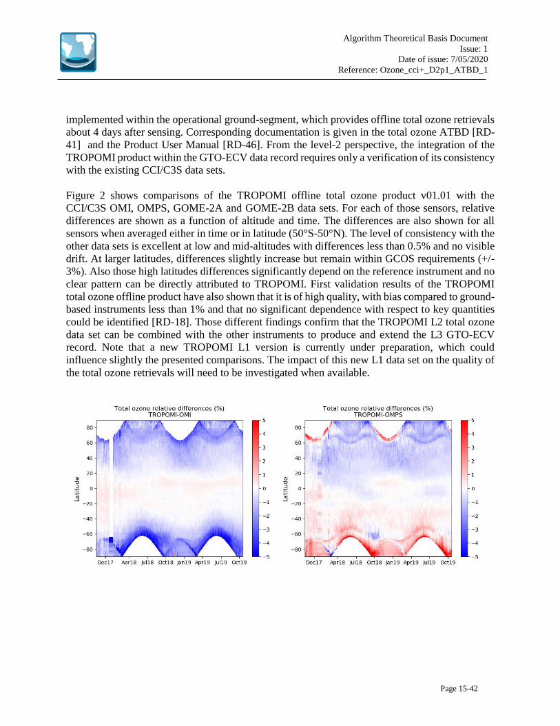
implemented within the operational ground-segment, which provides offline total ozone retrievals
about 4 days after sensing. Corresponding documentation is given in the total ozone ATBD [RD-
41] and the Product User Manual [RD-46]. From the level-2 perspective, the integration of the
TROPOMI product within the GTO-ECV data record requires only a verification of its consistency
with the existing CCI/C3S data sets.
Figure 2 shows comparisons of the TROPOMI offline total ozone product v01.01 with the
CCI/C3S OMI, OMPS, GOME-2A and GOME-2B data sets. For each of those sensors, relative
differences are shown as a function of altitude and time. The differences are also shown for all
sensors when averaged either in time or in latitude (50°S-50°N). The level of consistency with the
other data sets is excellent at low and mid-altitudes with differences less than 0.5% and no visible
drift. At larger latitudes, differences slightly increase but remain within GCOS requirements (+/-
3%). Also those high latitudes differences significantly depend on the reference instrument and no
clear pattern can be directly attributed to TROPOMI. First validation results of the TROPOMI
total ozone offline product have also shown that it is of high quality, with bias compared to ground-
based instruments less than 1% and that no significant dependence with respect to key quantities
could be identified [RD-18]. Those different findings confirm that the TROPOMI L2 total ozone
data set can be combined with the other instruments to produce and extend the L3 GTO-ECV
record. Note that a new TROPOMI L1 version is currently under preparation, which could
influence slightly the presented comparisons. The impact of this new L1 data set on the quality of
the total ozone retrievals will need to be investigated when available.
Algorithm Theoretical Basis Document
Issue: 1
Date of issue: 7/05/2020
Reference: Ozone_cci+_D2p1_ATBD_1
Page 16-42
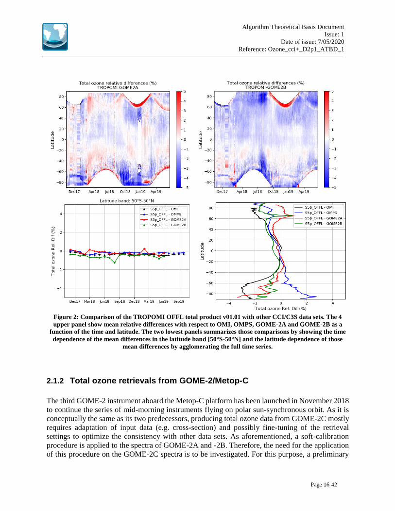
Figure 2: Comparison of the TROPOMI OFFL total product v01.01 with other CCI/C3S data sets. The 4
upper panel show mean relative differences with respect to OMI, OMPS, GOME-2A and GOME-2B as a
function of the time and latitude. The two lowest panels summarizes those comparisons by showing the time
dependence of the mean differences in the latitude band [50°S-50°N] and the latitude dependence of those
mean differences by agglomerating the full time series.
2.1.2 Total ozone retrievals from GOME-2/Metop-C
The third GOME-2 instrument aboard the Metop-C platform has been launched in November 2018
to continue the series of mid-morning instruments flying on polar sun-synchronous orbit. As it is
conceptually the same as its two predecessors, producing total ozone data from GOME-2C mostly
requires adaptation of input data (e.g. cross-section) and possibly fine-tuning of the retrieval
settings to optimize the consistency with other data sets. As aforementioned, a soft-calibration
procedure is applied to the spectra of GOME-2A and -2B. Therefore, the need for the application
of this procedure on the GOME-2C spectra is to be investigated. For this purpose, a preliminary

Algorithm Theoretical Basis Document
Issue: 1
Date of issue: 7/05/2020
Reference: Ozone_cci+_D2p1_ATBD_1
Page 17-42
process of the available L1 data has been carried out with GODFITv4 without any soft-calibration.
Figure 3 shows relative total ozone differences with respect to the columns measured by
TROPOMI as a function of time and latitude in the left panel. The right panel shows the time
dependence of those differences binned in different latitude bands. Overall, the differences are
quite small (<1%) for most latitudes. Nevertheless, they slightly increase at higher latitudes during
the local winter season. Although such larger differences are usually observed in those regions,
the low bias observed for GOME-2C might be a bit more important at high solar zenith angles.
Despite this concerns a limited range of geophysical conditions, we will further investigate this
during the second year of the project to better evaluate the level of consistency with the other data
sets and draw conclusions on the possible needs for retrieval optimization and/or for L1b soft-
calibration.
Figure 3: Comparison of the preliminary GOME-2C GODFITv4 total ozone product with the TROPOMI
OFFL total product v01. The left panel shows mean relative differences as a function of time and latitude. The
right panel shows the time dependence of mean differences in different latitude bands.
Algorithm Theoretical Basis Document
Issue: 1
Date of issue: 7/05/2020
Reference: Ozone_cci+_D2p1_ATBD_1
Page 18-42
2.2 GOME-type Total Ozone - Essential Climate Variable (GTO-ECV) (DLR)
2.2.1 Total ozone L3 algorithm
The individual level-2 total ozone observations as described in Sect. 2.1 are converted into a level-
3 product, i.e. they are mapped onto a regular global grid of 1°x1° in latitude and longitude to
construct daily averages for each sensor. Each grid cell contains an average of all level-2 data from
the same day, whose center coordinates fall in the respective grid cell.
2.2.2 Total ozone merging algorithm
Before combining the individual gridded daily level-3 data into a merged product, adjustments
are made in order to account for possible biases and drifts between the instruments. OMI
measurements serve as a baseline for the inter-sensor calibration. Their long-term stability with
respect to ground-based observation data is remarkable [RD-17] and the periods of overlap with
the other sensors are sufficiently long, i.e. at least 5 years. The calculation of the correction
factors for GOME, SCIAMACHY, GOME-2A, and GOME-2B with respect to OMI is based on
a comparison of 1° zonal monthly means during their overlap periods. The correction factors
depend on latitude and time and they are applied to the daily level-3 data. Subsequently, the
adjusted data sets are combined into one single record. All available daily measurements
(weighted by the number of measurements per day and grid box for the corresponding sensor)
are averaged. GOME and SCIAMACHY data are included until December 2004. Finally,
monthly means are computed taking into account the latitudinal constraints as defined in Table
xxx, in order to provide representative averages that contain a sufficient number of
measurements equally distributed over time (see also [RD-14]).
Month Latitudes Month Latitudes
January 60.0°N – 90.0°S July 90.0°N – 57.5°S
February 70.0°N – 90.0°S August 90.0°N – 62.5°S
March 80.0°N – 80.0°S September 82.5°N – 72.5°S
April 90.0°N – 65.0°S October 72.5°N – 85.5°S
May 90.0°N – 60.0°S November 65.0°N – 90.0°S
June 90.0°N – 57.5°S December 60.0°N – 90.0°S
2.2.3 GTO-ECV extension backward in time
For extending the GTO-ECV data record backward in time, we select the Adjusted-MERRA-2
reanalysis data set as described in [RD-15]. It covers the period from 1980 to 2018. We compare
5° zonal monthly means of GTO-ECV and Adjusted-MERRA-2 during the overlap period 1995-
2018 and compute corrections factors for the Adjusted-MERRA-2 data in order to calibrate them
with respect to GTO-ECV. The correction reduces potential biases between both data records. It
depends on latitude and month (January, February, ...) and is applied to the entire Adjusted-

Algorithm Theoretical Basis Document
Issue: 1
Date of issue: 7/05/2020
Reference: Ozone_cci+_D2p1_ATBD_1
Page 19-42
MERRA-2 data set starting in 1980. Finally, both data records are combined; we use the calibrated
Adjusted-MERRA-2 from 1980 through June 1995 and GTO-ECV from July 1995 to present.
Algorithm Theoretical Basis Document
Issue: 1
Date of issue: 7/05/2020
Reference: Ozone_cci+_D2p1_ATBD_1
Page 20-42
2.3 Multi-Sensor-Reanalysis scheme (KNMI)
2.3.1 Introduction MSR algorithm
A single coherent total ozone dataset, called the Multi Sensor Reanalysis (MSR), has been created
from all available ozone column data measured by polar orbiting satellites in the near-ultraviolet
Huggins band in the last thirty years. All available total ozone satellite retrieval datasets have been
used in the MSR. As first step a bias correction scheme is applied to all satellite observations,
based on independent ground-based total ozone data from the World Ozone and Ultraviolet Data
Center. The correction is a function of solar zenith angle, viewing angle, time (trend), and effective
ozone temperature. As second step data assimilation was applied to create a global dataset of total
ozone analyses. The data assimilation method is a sub-optimal implementation of the Kalman filter
technique, and is based on a chemical transport model driven by ECMWF meteorological fields.
The chemical transport model provides a detailed description of (stratospheric) transport and uses
parameterisations for gas-phase and ozone hole chemistry. The MSR dataset is available on a grid
of a 0.5x0.5 degrees with a sample frequency of 6 hours for the complete time period.
Constructing the MSR level 2 data set
Creating a consistent and coherent assimilated dataset of use for trend studies requires that
systematic offsets of each one of the satellite retrieval products is small. A practical way to
accomplish this is to choose a reference dataset which is available for the full reanalysis period,
and subsequently correct the systematic effects in the satellite datasets to bring them in line with
this reference. As reference we use the ground measurements from Brewer and Dobson monitoring
stations, which are present for the full 30-year period.
First of all, these ground measurements will also show biases, depending on geometry,
meteorological variability and ozone profile. The direct Sun measurement method used by the
Brewer instruments is very sensitive to small details in the ozone absorption cross section, and the
various available laboratory measurements of the ozone absorption coefficients give totally
different dependencies of the retrieved total ozone values as function of the effective ozone
temperature [RD-34]. Kerr (2002) [RD-22] has developed a new methodology for deriving total
ozone and effective ozone temperature values from the observations made with a Brewer
instrument. He concludes that the effective ozone temperature has little effect on the amount of
ozone derived with the standard algorithm. So in this study the data from the Brewer network has
been adopted as a primary reference. The Dobson data compared to Brewer data show a
temperature dependence. Therefore, the Dobson data has been corrected for effective ozone
temperature and added to this reference data set.
Algorithm Theoretical Basis Document
Issue: 1
Date of issue: 7/05/2020
Reference: Ozone_cci+_D2p1_ATBD_1
Page 21-42
For each satellite product an “overpass” dataset has been created for each ground instrument in
our list. The overpass value for an orbit is the satellite observation that has the centre of its footprint
closest to the ground station. For each satellite product a maximum allowed distance between the
centre of the ground pixel and the ground station was defined. This number is typically 50-200 km
depending on the ground pixel size. Apart from the local date/time and the total ozone value,
auxiliary data is also recorded, like the measurement error, the Solar Zenith Angle (SZA), the
Viewing Zenith Angle (VZA), cloud properties and the distance from the centre of the footprint to
the ground station. From all the overpasses each day only one is selected and used. This is the one
with the smallest reported observation error or the one closest to the ground station if the
observation error is not available.
For the purpose of data assimilation it is relevant to reduce offsets, trends and long-term variations
in the satellite data, so that the data can be used as input to the assimilation scheme without biases
and with known standard deviations. The satellite data set corrections are based on a few relevant
regression coefficients fitted for the overpass time series of all stations together. By fitting all data
together regional biases that may be caused by offsets of individual ground instruments are
avoided.
The ozone differences (satellite minus ground observation) show a clear seasonal cycle. This led
to the choice of SZA and effective ozone temperature as fit parameter, as these imply a clear
seasonal component. Some of the satellite products show a clear trend in time, so date/time is
another obvious choice. The Viewing Zenith Angle (VZA) is also used as fit parameter. These are
all critical parameters in the retrieval schemes and therefore constitute a satisfying choice to
estimate systematic biases. A ground-station dependent offset was allowed when the regression
coefficients were computed. This has been done to reduce the effect (e.g. spurious trends) of
“appearing” and “disappearing” ground stations during the lifetime of the satellite instrument from
the results. Thus, the total number of fit parameters is in the order of 150 per satellite dataset. A
basic assumption is that all the corrections are additive to the total ozone amount.
Based on the calculated corrections the merged MSR level 2 dataset has been created. The original
satellite datasets were read, filtered for bad data and corrected, and finally merged into a single
time ordered dataset. Essential information in the MSR level 2 dataset is time, location, satellite
product index and ozone.
Data assimilation
The satellite instrument observations are combined with meteorological, chemical and dynamical
knowledge of the atmosphere by using data assimilation. The data assimilation scheme used here
is called TM3DAM and is described in Eskes et al. (2003). The chemistry-transport model used in
this data assimilation is a simplified version of TM5 [RD-24], which is driven by ECMWF
analyses of wind, pressure and temperature fields. As input the MSR ozone values and the
estimates of the measurement uncertainty are used.
Algorithm Theoretical Basis Document
Issue: 1
Date of issue: 7/05/2020
Reference: Ozone_cci+_D2p1_ATBD_1
Page 22-42
The three-dimensional advection of ozone is described by the flux-based second order moments
scheme of Prather et al. (1986) [RD-32]. The model is driven by 6-hourly meteorological fields
(wind, surface pressure, and temperature) of the medium-range meteorological analyses of the
ECMWF. The assimilation is using the ERA interim or ERA5 reanalysis whenever available. The
ECMWF hybrid layers between 0.01 hPa and the surface have been converted into the 44 layers
used in TM3DAM. The horizontal resolution of the model version used in this study is 1 x 1
degrees. This resolution is compensated by the practically non-diffusive Prather scheme (with 10
explicit ozone tracers for each grid cell), which allows the model to produce ozone features with a
fair amount of detail.
Ozone chemistry in the stratosphere is described by the Cariolle version 2.9 parameterisation [RD-
11]. This consists of a linearization of the gas-phase chemistry with respect to production and loss,
the ozone amount, temperature and UV radiation. In addition, a second parameterization scheme
accounts for heterogeneous ozone loss. This scheme introduces a three-dimensional chlorine
activation tracer, which is formed when the temperature drops below the critical temperature of
polar stratospheric cloud formation. Ozone breakdown occurs in the presence of the chlorine
activation tracer, depending on the presence of sunlight. The rate of ozone decrease is described
by an exponential decay, with a rate proportional to the amount of activation tracer below the
critical temperature and with a minimal decay time of 12 days. The cold tracer is deactivated when
light is present with a time scale of respectively 5 and 10 days on the Northern and Southern
hemisphere.
The total ozone data are assimilated in TM3DAM by applying a parameterized Kalman filter
technique. In this approach the forecast error covariance matrix is written as a product of a time
independent correlation matrix and a time-dependent diagonal variance. The various parameters
in the approach are fixed and are based on the forecast minus observation statistics accumulated
over the period of one year (2000) using GOME observations. This approach produces detailed
and realistic time- and space-dependent forecast error estimates, which is included in the MSR
level 4 product.
More details of the MSR algorithm can be found in [RD-43] and [RD-42].
2.3.2 Algorithm update to extend the MSR data set into the past
Heterogeneous chemistry
An EESC dependent heterogeneous chemical destruction of stratospheric ozone factor has been
be incorporated within the exponent of the ozone depletion term within the Braesicke scheme.
The EESC correction factor fCFC is calculated according
FCFC = (EESC/EESCmax)2 where EESCmax = 4092.8508
Algorithm Theoretical Basis Document
Issue: 1
Date of issue: 7/05/2020
Reference: Ozone_cci+_D2p1_ATBD_1
Page 23-42
The EESC values are derived in [RD-29] and are calculated for the period 1957-2020.
Solar Zenith Angle dependence of photolysis factor
A linear correction factor fSZA for photolysis during twilight has been derived. The twilight is the
zone with a Solar Zenith Angle (SZA) between 85 and 94 degree.
fSA = (94.0 – SZA)/(94.0 – 85.0) for SZA between 84.0-95.0 degree
This factor has been multiplied with the chlorine activation term.
Error correlation length
For sparse observations it is likely that the error correlation length in the spatial distribution of
assimilated ozone is different. Therefore the correlation length is determined by assimilating ozone
using only sparse Dobson observations in 2017. The resulting ozone has been compared with the
MSR2 ozone distribution that represent the “true” ozone distribution. From analysing these
datasets we conclude that the correlation length is about 800 km.
Algorithm Theoretical Basis Document
Issue: 1
Date of issue: 7/05/2020
Reference: Ozone_cci+_D2p1_ATBD_1
Page 24-42
3 Nadir Profile ECV Retrieval Algorithms
3.1 RAL nadir profile ECV retrieval algorithms (RAL)
The RAL profile scheme applied to GOME, GOME-2, SCIAMACHY and OMI within the CCI
and C3S is described in ATBDs [RD-46], [RD-45], as well as [RD-27], [RD-35] and [RD-27].
The scheme is also currently being developed for application to Sentinel 4 and 5 via ESA contracts
and documented via related ATBDs [RD-38] and [RD-36]. In general, the scheme applies the
optimal estimation approach to retrieve the ozone profile in two main steps:
1. “B1 fit”: Fit ozone profile to the sun-normalised radiance in the Harley band (in GOME
Band 1) from 265-307nm. This provides information mainly on the stratospheric profile
and requires good absolute calibration of the sun-normalised radiance spectra. Soft
calibration of the B1 L1 radiances in usually required (i.e. radiances are corrected based on
differences between L1 radiances and calculated spectra based on radiative transfer
calculations from prior knowledge of the ozone distribution).
2. “B2 fit”: Add information on tropospheric ozone from the Huggins bands (320-340nm)
using the result from step 1) as prior constraint. This requires fitting of differential structure
to precision better than 0.1% (close to the noise level) to allow the ozone absorption cross-
section temperature dependence to be exploited for tropospheric information (though the
requirements on absolute radiometic calibration are less stringent). Extremely good
knowledge of the instrument spectral response function is critical for this step.
Work within CCI+ focuses on the application of the algorithm to new sensors GOME-2 Metop C
and S5P. For S5P several advances made for Sentinel 4 and 5 will be exploited, in particular:
The core radiative transfer model is LIDORT [RD-39].
The speed of the forward model is greatly increased using a “PCFM” approach which
requires the core RTM to be run for only a few monochromatic spectral points.
The B1 uv soft-calibration approach will be based on that developed for S5 [RD-36], based
on calculations based on ERA5 meteorology and ozone climatology.
A new approach to mitigate scene inhomogeneity effects on the spectral response function
will be tested using an approach developed for S4 [RD-38].
Algorithm Theoretical Basis Document
Issue: 1
Date of issue: 7/05/2020
Reference: Ozone_cci+_D2p1_ATBD_1
Page 25-42
3.2 IASI FORLI Ozone profile retrieval algorithm (ULB) The IASI ozone profile data product is based on the FORLI (Fast Optimal/Operational Retrieval
on Layers for IASI) algorithm. FORLI is a line-by-line radiative transfer model capable of
processing in near-real-time the numerous radiance measurements made by the high-spatial and
high-spectral resolution IASI, with the objective to provide global concentration distributions of
atmospheric trace gases.
The FORLI-O3 v20151001 product was developed and validated during the Ozone_cci Phase-II
and constitutes the reference product from 1rst October 2007 to 11 December 2019. That
IASI/Metop-A FORLI-O3 dataset has been extensively validated in [RD-10] and [RD-21].
An updated FORLI-O3 v20191122 is now used for the processing of the IASI dataset from 12
December 2019 till present. The FORLI-O3 datasets processed with FORLI-O3 v20151001 and
v20191122 for IASI-A, -B and –C can be downloaded from the Aeris portal at: http://iasi.aeris-
data.fr/O3/. The backprocessing of the whole IASI dataset with the last v20191122 is ongoing and
will be archived on the Aeris portal in the future.
This part describes the methods used for FORLI (most is extracted from [RD-20]) and is an update
of the Ozone_cci ATBD Phase-II. We refer the readers to the Ozone_cci ATBD Phase-II when the
section remains unchanged.
3.2.1 Basic retrieval equations
Refer to the Ozone_cci_ATBD_Phase2_V2
3.2.2 Assumptions, grid and sequence of operations
Spectral ranges FORLI-O3 (v20151001 and v20191122) uses the Level1C radiances disseminated by EumetCast.
A subset of the spectral range, covering 1025–1075 cm 1 , is used for the O3 retrieval. The spectral
range used in the forward model is 960-1075 cm-1 and the spectral oversampling is 100.
Vertical grid FORLI-O3 uses a vertical altitude grid in km with 1-km tick layers as discretization of the
atmosphere
Ozone state vector The ozone product from FORLI is a profile retrieved on 40 1km-thick layers between surface and
40 km, with an extra layer from 40 to TOA considered at 60 km.
Algorithm Theoretical Basis Document
Issue: 1
Date of issue: 7/05/2020
Reference: Ozone_cci+_D2p1_ATBD_1
Page 26-42
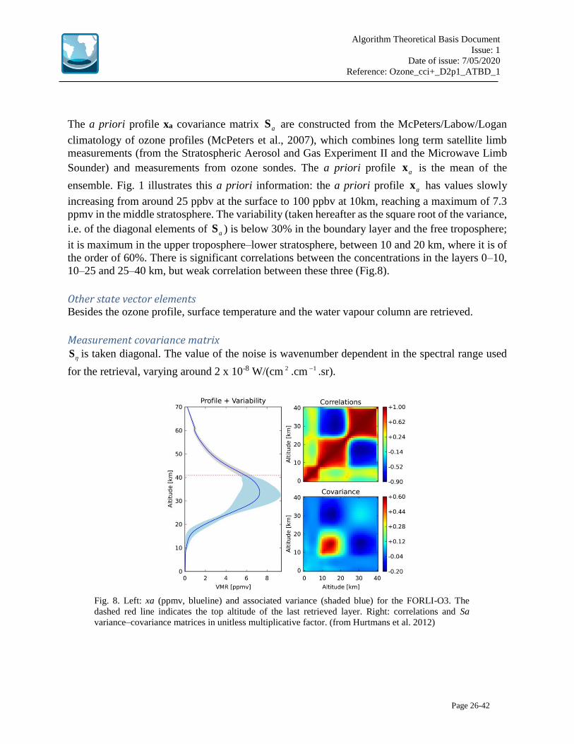
The a priori profile xa covariance matrix aS are constructed from the McPeters/Labow/Logan
climatology of ozone profiles (McPeters et al., 2007), which combines long term satellite limb
measurements (from the Stratospheric Aerosol and Gas Experiment II and the Microwave Limb
Sounder) and measurements from ozone sondes. The a priori profile ax is the mean of the
ensemble. Fig. 1 illustrates this a priori information: the a priori profile ax has values slowly
increasing from around 25 ppbv at the surface to 100 ppbv at 10km, reaching a maximum of 7.3
ppmv in the middle stratosphere. The variability (taken hereafter as the square root of the variance,
i.e. of the diagonal elements of aS ) is below 30% in the boundary layer and the free troposphere;
it is maximum in the upper troposphere–lower stratosphere, between 10 and 20 km, where it is of
the order of 60%. There is significant correlations between the concentrations in the layers 0–10,
10–25 and 25–40 km, but weak correlation between these three (Fig.8).
Other state vector elements Besides the ozone profile, surface temperature and the water vapour column are retrieved.
Measurement covariance matrix
S is taken diagonal. The value of the noise is wavenumber dependent in the spectral range used
for the retrieval, varying around 2 x 10⁻⁸ W/(cm 2 .cm 1 .sr).
Fig. 8. Left: xa (ppmv, blueline) and associated variance (shaded blue) for the FORLI-O3. The
dashed red line indicates the top altitude of the last retrieved layer. Right: correlations and Sa
variance–covariance matrices in unitless multiplicative factor. (from Hurtmans et al. 2012)

Algorithm Theoretical Basis Document
Issue: 1
Date of issue: 7/05/2020
Reference: Ozone_cci+_D2p1_ATBD_1
Page 27-42
3.2.3 Iterations and convergence
Refer to Ozone_cci_ATBD_Phase2_V2
3.2.4 Forward model
Atmospheric state input to the RTM
L1C radiances FORLI-O3 uses the Level1C radiances disseminated by EumetCast. A subset of the spectral range,
covering 1025–1075 cm 1 , is used for the O3 retrieval.
Temperature and humidity profiles Profiles of temperature and humidity are from the IASI L2 PPF (August et al., 2012). The
atmospheric temperatures are kept fixed whereas the water profile is used as a priori and further
adjusted.
Surface temperature Surface temperatures (land and sea) are from the IASI L2 PPF. Surface temperature is part of the
parameters to be retrieved.
Cloud fraction FORLI-O3 uses the cloud fraction from the IASI L2 PPF. All pixels with a cloud fraction equal to
or lower than 13 % are processed.
CO2 profile FORLI-O3 v20151001 assumes a constant vertical profile at 380 ppm for CO2, while the new
FORLI-O3 v20191122 considers time-varying CO2 concentrations according to the Keeling curve.
Orography Orography is from the GTOPO30 global digital elevation model and is integrated in the entire
IASI FOV (http://eros.usgs.gov/#/Find_Data/Products_and_Data_Available/gtopo30_info).
Emissivity A wavenumber-dependent surface emissivity above continental surfaces is used while for ocean a
single standard emissivity is considered. For continental surfaces, it relies on the climatology of
Zhou et al. (2011). In cases of missing values in the Zhou et al. climatology, the MODIS
climatology of Wan (2008) is used. It is available on a finer 0.05° 0.05° grid but is restricted to
only 12 channels in the IASI spectral range. In order to deal with this, the spectrally resolved mean
emissivity of the Zhou climatology is scaled to match as closely as possible the values in these 12
channels and it is this resulting emissivity that is considered. Finally when there is no
correspondence between the IASI FOV and either climatologies, then the mean emissivity of the
Zhou climatology is used.

Algorithm Theoretical Basis Document
Issue: 1
Date of issue: 7/05/2020
Reference: Ozone_cci+_D2p1_ATBD_1
Page 28-42
Lookup-tables Tabulated absorption cross-sections at various pressures and temperatures are used to speed up the
radiative transfer calculation. The spectral range for the LUTs used in FORLI-O3 is 960-1075 cm-
1 and the spectral oversampling is 100. The absorption cross-sections are computed on a
logarithmic grid for pressure from 4.510-5 to 1 atm with a grid step of 0.2 for the logarithm of
pressure, and on a linear grid for temperature (162.8–322.6 K with a grid step of 5K). Relative
humidity is also introduced in the LUT, varying linearly between 0 and 100%, by steps of 10%.
The FORLI-O3 v20191122 has undergone corrections in the computation of the look-up tables.
Spectroscopy Line integrated absorption cross section, air broadening, self-broadening, line shifting and
absorption cross section data are taken from the widely used HITRAN spectroscopic database
version 2008 (Rothman et al., 2009). Continuum formulations are taken from MT-CKD (Clough
et al., 2005).
The last FORLI version (v20191122) uses the Hitran database update to the latest available version
with largely corrected CO line intensities and positions and also updates for HNO3, as well as
MT_CKD update and the related use of Line-Mixing for CO2 lines.
Note that other corrections have also been implemented in FORLI-O3 v20191122: altitudes
computation, correct usage of humidity …
Radiative Transfer Model (RTM)
Refer to Ozone_cci_ATBD_Phase2 for a full description of the RTM (general formulations and
numerical approximations).
3.2.5 Error description
Refer to Ozone_cci_ATBD_Phase2.
3.2.6 Output product description
Formats The FORLI-O3 retrieval datasets for IASI-A, -B and -C processed with FORLI-O3 v20151001
from 1rst October 2007 to 11 December 2019 and processed with FORLI-O3 v20191122 from 12
December 2019 till present will be delivered in NetCDF (v4) format and can be downloaded from
the Aeris portal at: http://iasi.aeris-data.fr/O3/.
Algorithm Theoretical Basis Document
Issue: 1
Date of issue: 7/05/2020
Reference: Ozone_cci+_D2p1_ATBD_1
Page 29-42
Ozone profile and characterization The ozone product from FORLI is a profile retrieved on 40 layers between surface and 40 km,
with an extra layer from 40 km to the top of the atmosphere (TOA) considered at 60 km. The
dataset includes O3 total columns along with vertical profiles. It also includes other relevant
information such as the a priori profile, the total error profile and the averaging kernel (AK) matrix,
on the same vertical grid.
3.2.7 Retrievals and Quality flags
A series of Quality input and processing flags were applied to the FORLI-O3 datasets (v20151001
and v20191122) to exclude bad quality data, specifically when:
(i) The input values (T, Q, Cloud) are missing, or in case of negative surface altitudes or
unrealistic skin temperature
(ii) The spectral fit residual root mean square error (RMS) is higher than 3.5×10⁻⁸ W/(cm2
sr cm−1), reflecting a too large difference between observed and simulated radiances
(iii) The spectral fit residual bias is lower than -0.75 x 10⁻⁹ W/(cm2 sr cm−1) or higher than
1.25 x 10⁻⁹ W/(cm2 sr cm−1)
(iv) The spectral fit residual is sloped
(v) The partial O3 column or the humidity is negative
(vi) There were abnormal averaging kernel values
(vii) The spectral fit diverged or reached a fixed maximum number of iterations without
converging, or the Chi-Square value is too high
(viii) The total error covariance matrix is ill conditioned.
(ix) No retrieval is done due to incorrect inputs or other reasons
For an optimal use of the data (e.g. for validation application), users should also exclude data
when:
(i) The O3 profiles have an unrealistic C-shape (i.e. abnormal increase in O3 at the surface,
e.g. over desert due to emissivity issue), with a ratio of the surface – 6 km column to
the total column higher or equal to 0.085
(ii) The DOFS is lower than 2, which are mostly associated with bad quality data in the
Antarctic region.
The IASI/Metop-A, -B and -C O3 dataset are provided on the Aeris portal on the global scale from
October 2007 till present.
Algorithm Theoretical Basis Document
Issue: 1
Date of issue: 7/05/2020
Reference: Ozone_cci+_D2p1_ATBD_1
Page 30-42
3.3 Combined uv/vis/thermal-ir retrieval algorithm (RAL)
3.3.1 Overview
Within CCI+ (mainly in year 2) RAL will investigate improve the information content of the GOME-
2 nadir ozone profiles by adding information from (i) the visibile Chappuis band (also measured by
GOME-2) and (ii) thermal IR measurements by IASI (ii). The approach is to combine information
from indendent level 2 (L2) retrievals from the different spectral ranges, i.e. adopting a so-called “L2-
L2” combination approach. Sections below described the Chappuis and IR retrieval schemes to be
employed, following by an overview of the L2 combination methodology.
3.3.2 Chappuis retrieval scheme
The potential advantages of using the Chappuis bands (440-700nm) are well known [RD-12]: The
Chappuis absorption is generally optically thin with very little temperature dependence. There is
consequently little sensitivity to vertical profile shape (only total column information can be
retrieved from the Chappuis band alone). However it can complement the uv measurements of
total ozone because near-ground sensitivity to ozone in the Huggins bands is limited by the
typically low surface reflectance and Rayleigh / aerosol scattering. In the Chappuis range, the
albedo over land is typically larger and Rayleigh scattering much reduced, so that a larger
proportion of the observed photons will have passed through the lowest atmospheric layers.
Extracting the signal from the Chappuis bands is complicated by the fact that the amplitude of
differential structures (which are exploited by DOAS techniques) are relatively low and have a
relatively broad band structure compared to the features in the Huggins bands. Such features may
be easily confused with a number of other effects e.g. instrumental artefacts (such as polarisation
sensitivity, aliasing of spatial/spectral structure due to non-synchronous detector pixel read-out)
and spectral variations in surface reflectance. In addition, there are contaminating spectral features
from water vapour (H2O), oxygen dimer (O4) and nitrogen dioxide (NO2). Although Rayleigh
scattering is reduced, the Ring effect (due to inelastic scattering by air molecules) is still
significant. Inelastic scattering at the ocean surface is also important over sea, although in
conditions where this is important, the information content of the Chappuis bands is less useful (as
the ocean surface reflection is very low).
Via UK National Centre for Earth Observation (NCEO) funded work (to be consolidated in the
coming months) two approaches have been developed to extract the total (slant) column of ozone
from the Chappuis: (1) A DOAS based approach, which has a directly physical basis. This involves
fitting absorption cross sections for all relevant gases and scale factors for terms related to known
surface spectral variability and other known effects (Ring effect, spectral shifts, instrument
polarisation features etc); (2) A statistical approach based on regressing the Chappuis band
measurements to the ozone slant column retrieved from the Huggins bands. This involves
determine singular vectors of the Chappuis band spectral variability which is uncorrelated with the
total ozone variability enabling total ozone to be retrieved along with spatial patterns which are
related to other physical variables. In both cases the slant column of ozone is estimated. The
Algorithm Theoretical Basis Document
Issue: 1
Date of issue: 7/05/2020
Reference: Ozone_cci+_D2p1_ATBD_1
Page 31-42
sensitivity of the slant column to height resolved perturbations in ozone can be calculated, forming
effectively the averaging kernel of the retrieved slant column with respect to changes in ozone
profile. This information can then be combined with the uv retrieval using the L2-L2 approach
outlined below.
Further details of the consolidated approach will be given in the next version of this ATBD.
3.3.3 RAL Infra-red / Microwave sounder retrievals
Also within NCEO and supported by Eumetsat studies, RAL have developed an infra-red
microwave sounder (IMS) scheme which retrieves ozone profiles along with temperature,
humidity and other atmospheric variables from Metop IASI, AMSU and MHS. Products from the
scheme have been validated in CCI+ Water Vapour and will be used to generate a combined
limb/nadir sounder product in that project. The scheme is described in the CCI+ water vapour
ATBD [RD-37], though the current version of the scheme uses an extended set of channels to
improve the sensitivity to the ozone profile. The scheme is based on optimal estimation and
provides all the necessary information to enable L2-L2 combination with the uv profiles as
described below.
3.3.4 L2-L2 Combination
The L2-L2 combination is implemented by posing the problem as a linear retrieval in which we
wish to optimally estimate a profile by combining the information contained in different retrievals.
The approach should work for a retrieval of any property linearly related to the profile e.g.
(sub-)column amounts or mixing ratio profiles on a coarsely sampled vertical grid (provided the
transformation to a fine grid is clearly defined). For the approach to work, it is assumed that
averaging kernels are provided (or can be constructed) for all input retrievals, with respect to fine
scale perturbations in the true profile (defined in the same units on the same finely resolved grid).
We choose to represent the (output, optimised) profile in a flexible way on a fine vertical grid
using N basis functions (this can be different from the way the input retrievals represent the
profile):
𝒓(𝑧) = 𝑜(𝑧) + ∑ 𝑥𝑖𝐵𝑖(𝑧)
𝑖=1,𝑁
Equation 1
Where 𝑜(𝑧) is an “offset” profile (which can be considered as the new prior profile on the fine
grid). 𝐵(𝑧) are a set of suitable basis functions (e.g. triangular functions representing linear
interpolation from a coarse vertical grid, or principal components of the assumed profile variability
etc). The N element vector 𝒙 contains state vector elements to be retrieved.
Algorithm Theoretical Basis Document
Issue: 1
Date of issue: 7/05/2020
Reference: Ozone_cci+_D2p1_ATBD_1
Page 32-42
Alternatively, considering vector 𝒓 to describe the profile on a finely resolved vertical grid:
𝒓 = 𝒐 + 𝑩𝒙
Equation 2
Where B is a matrix containing the N basis functions.
The optimal 𝒙 (and hence 𝒓) can be obtained using the input retrievals as the “measurements” for
an OEM retrieval. These are contained in a measurement vector, 𝒚. We can relate each to 𝒙, using
the averaging kernels as the forward model function:
𝑦𝑗 = 𝑨𝑗(𝒓 − 𝒓𝒂𝒋) + 𝑎𝑗
Equation 3
Where index j represents a specific sub-column amount (from TIR or SWIR). 𝑨𝒋 is the averaging
kernel (vector) for this sub-column (from the TIR or SWIR retrieval), describing the derivative of
the sub-column with respect to perturbations on the fine grid. 𝒓𝒂𝒋 is the (finely resolved) prior
profile used in the previous (input) retrieval and 𝑎𝑗 is the corresponding prior sub-column amount.
Substituting for 𝒓 gives
𝑦𝑗 = 𝑨𝑗(𝒐 + 𝑩𝒙 − 𝒓𝒂𝒋) + 𝑎𝑗
Equation 4
Using this (linear) forward model for 𝐹(𝑥), 𝒙 can be estimated via minimisation of the usual cost
function, 𝜒2, i.e.
𝜒2 = (𝒙 − 𝒙𝒂)𝑇𝑺𝑎−1(𝒙 − 𝒙𝑎) + (𝒚 − 𝐹(𝒙))
𝑇𝑺𝑒
−1(𝒚 − 𝐹(𝒙)), Equation 5
Where the measurement covariance 𝑺𝒆 constains the estimated error covariances of the
(TIR+SWIR) subcolumns in 𝒚. A priori covariance 𝑺𝒂 describes the estimated prior errors on the
state vector (i.e. the basis function weights). In principle these are defined to represent realistic
prior knowledge in the profile, though tuning to match the information content of the joint retrieval
is likely to be needed in practise. The prior state itself, 𝒙𝑎 , is typically a vector of 0s, since the
state describes increments to the offset profile, 𝒐.
Since the forward model is linear, the solution which minimises the cost function is given by
�̂� = 𝒙𝒂 + ( 𝑲𝑻𝑺𝒆−𝟏𝑲 + 𝑺𝒂
−𝟏 )−1
𝑲𝑇𝑺𝒆−𝟏 ( 𝒚 − 𝐹(𝒙𝒂))
Equation 6
where weighting function matrix 𝑲 is the derivative of the forward model with respect to the state
parameters, i.e.
𝑲 = 𝑨 𝑩

Algorithm Theoretical Basis Document
Issue: 1
Date of issue: 7/05/2020
Reference: Ozone_cci+_D2p1_ATBD_1
Page 33-42
Equation 7
Where A is the matrix containing the averaging kernels of the input retrieved amounts with respect
to the fine scale profile (columns are 𝑨𝑗 in Equation 4). Note that (assuming linearity), using the
averaging kernel equation as the forward model operator, effectively removes the influence of the
original retrievals prior constraint on the joint retrieval (this is effectively replaced by the new
prior).
Given the solution state, it is trivial to compute the corresponding high-resolution version of the
profile, 𝒓 (Equation 2). Sub-column amounts for specific layers can then be calculated from that
profile. This step can be carried out by matrix multiplication by matrix, 𝑴, which contains the
weights needed to integrated the profile to a set of sub-column amounts, such that
𝒔 = 𝑴 𝒓 Equation 8
Via the usual OEM equations, the total a posteriori errors on �̂� are described by covariance
𝑺𝒙 = ( 𝑲𝑻𝑺𝒆−𝟏𝑲 + 𝑺𝒂
−𝟏 )−1
Equation 9
The (non-square) averaging kernel for �̂�, giving derivatives of the solution with respect to fine-
scale perturbations in the profile is given by
𝑨𝒙 = 𝑺𝒙𝑲𝑻𝑺𝒆−𝟏𝑨
Equation 10
(𝑨, without subscript, is the derivative of the input retrievals with respect to fine-scale
perturbations in the true profile).
The (square) averaging kernel for the output fine scale profile is:
𝑨𝒓 = 𝑩𝑨𝒙 Equation 11
The (non-square) averaging kernel for the derived sub-columns (with respect to fine scale
perturbations in the profile) is
𝑨𝒔 = 𝑴𝑨𝒓 Equation 12
Errors on the retrieval profile and sub-columns are described by covariances:
𝑺𝒓 = 𝑩𝑺𝒙𝑩𝑻

Algorithm Theoretical Basis Document
Issue: 1
Date of issue: 7/05/2020
Reference: Ozone_cci+_D2p1_ATBD_1
Page 34-42
Equation 13
𝑺𝒔 = (𝑴𝑩)𝑺𝒙(𝑴𝑩)𝑻
Equation 14
(The noise and smoothing error covariances can be similarly derived starting from the usual OEM
expression for these matrices for the state vector �̂�).
Algorithm Theoretical Basis Document
Issue: 1
Date of issue: 7/05/2020
Reference: Ozone_cci+_D2p1_ATBD_1
Page 35-42
4 Limb profile ECV Retrieval / Merging Algorithm
4.1 HARMonized dataset of OZone profiles (HARMOZ) (Bremen) The concept of the HARMonized dataset of OZone profiles (HARMOZ) is based on limb
and occultation measurements has been developed in the Ozone_CCI project (Sofieva et al., 2013).
HARMOZ consists of original retrieved ozone profiles from each satellite instrument, which are
screened for invalid data by the instrument teams. While the original ozone profiles are presented
in different units and on different vertical grids, the harmonized dataset is given on a common
vertical grid in netcdf-4 format. The vertical range of the ozone profiles is specific for each
instrument, thus all information contained in the original data is preserved. Provided altitude and
temperature profiles allow the representation of ozone profiles in number density or mixing ratio
on a pressure or altitude vertical grids. Geolocation, uncertainty estimates and vertical resolution
are provided for each profile. For each instrument, optional parameters, which are related to the
data quality, are also included.
In the CCI project, two versions of the HARMOZ datasets are developed and created: altitude-
gridded (HARMOZ_ALT) and pressure-gridded (HARMOZ_PRS) ozone concentration datasets.
The vertical sampling of HARMOZ_ALT profiles is 1 km. For HARMOZ_PRS, the pressure grid
corresponds to vertical sampling of ~1 km below 20 km and 2-3 km above 20 km. The information
about the available HARMOZ datasets is collected in Table 4.1. The datasets, which are developed
or extended in CCI + project, are highlighted.
Table 4.1 Information about the HARMOZ_ALT and HARMOZ_PRS dataset
Instrument/ satellite Level 2
processor Years Vertical range
Retrieval
vertical
coordinate MIPAS/Envisat KIT/IAA
V7R_O3_240
2002-2012 6-70 km/400- 0.05 hPa altitude
SCIAMACHY/Envisat UBr v3.5 2002-2012 5-65 km/250 – 0.05 hPa altitude
GOMOS/Envisat ALGOM2s v1 2002-2011 10-105 km/250- 10-4 hPa altitude
GOMOS bright limb/
Envisat
GBL v1.2 2002-2011 10-59 km/70 – 0.2 hPa altitude
POAM III/SPOT 4 NASA, v4 1998-2005 6-55 km /500 - 0.1 hPa altitude
SAGE III Meteor 3M NASA, AO3 v4 2002-2005 6-60 km /500 - 0.05 hPa altitude
OSIRIS/Odin USask v5.10 2001-2019 10-59 km/450 - 0.1 hPa altitude
ACE-FTS/SCISAT UoT v3.5/3.6 2004-2019 10-94 km/450 - 2⋅ 10-4
hPa
altitude
OMPS-LP/Suomi-NPP USask 2D v1.1.0 2012-2019 6-59 km/500 - 0.1 hPa altitude
MLS/Aura NASA_JPL v4.2 2004-2019 6-75 km /500 - 0.02 hPa pressure
SABER/Timed NASA_GATS v2 2002-2019 12-105 km/400- 1⋅ 10-4
hPa
pressure
SAGE III ISS NASA, AO3 v5.1 2017-2019 6-60 km /500 - 0.05 hPa altitude

Algorithm Theoretical Basis Document
Issue: 1
Date of issue: 7/05/2020
Reference: Ozone_cci+_D2p1_ATBD_1
Page 36-42
The dataset is available at http://dx.doi.org/10.5270/esa-ozone_cci-limb_occultation_profiles-
2001_2012-v_1-201308.
Algorithm Theoretical Basis Document
Issue: 1
Date of issue: 7/05/2020
Reference: Ozone_cci+_D2p1_ATBD_1
Page 37-42
4.2 OMPS Retrieval Schemes (Bremen)
4.2.1 OMPS-LP NASA retrieval algorithm version 2.5
The NASA Environmental Data Record algorithm to retrieve ozone profiles from OMPS-LP
measurements is based on the optimal estimation approach. Several versions of the retrieval
algorithm were released starting from April 2012; the most recent version 2.5 is described in
Kramarova et al. (2018). In this version, to improve the stability of the retrieval, a correlation
radius of 5 km was introduced in the a priori covariance matrix instead of the previously employed
Tikhonov parameter. To simulate limb radiance, the Gauss-Siedel radiative transfer model is used
and the Bass and Paur ozone cross section selected.
The algorithm is designed to retrieve ozone independently from two spectral ranges: the UV region
between 28.5 and 52.5 km and the Chappuis band between 12.5 (or cloud top height) and 37.5 km.
The doublet and triplet method is used to obtain the measurement vector, respectively, for the
Hartley-Huggins and Chappuis bands. Wavelengths characterized by a strong ozone absorption
are paired with weak absorbing ones. The normalization of the radiance is performed using an
upper tangent height measurement: 55.5 km in the UV and 40.5 km in the Vis. An additional TH
correction is applied by NASA on L1 gridded data, as described in Kramarova et al. (2018). A new
algorithm was developed to detect the cloud top height (Chen et al. 2016) and accordingly filter
out underneath THs. In addition, aerosol extinction profiles are currently derived for each
measurement, replacing the climatology profiles used in the previous versions, as described in
Loughmann et al. (2018).
Only the central slit of the instrument is considered and currently provided in L2 NASA product,
because of the uncertainties in the pointing and stray light issues affecting the two side slits.
4.2.2 OMPS-LP IUP retrieval algorithm version 2
In the UBR-IUP retrieval version five spectral segments are selected: three in the Hartley and
Huggins bands and two in the visible spectral range. We have to take into account the presence of
water vapor and O2 absorption features in the Chappuis band used for the lowest altitude range (*)
so that wavelengths in the intervals 585-605 nm and 620-635 nm are rejected. The treatment of
these absorption features requires line-by-line calculations, which are computationally expensive
to be implemented for the whole time series.
Considering the decreasing sensitivity above 55 km and the saturation of limb signal in the lower
stratosphere, the retrieval of ozone profiles is performed over the altitude range between 12 and
60 km, with the lower boundary that can be higher in the presence of a cloud. An evenly spaced
vertical grid spans this vertical range with steps every 1 km.
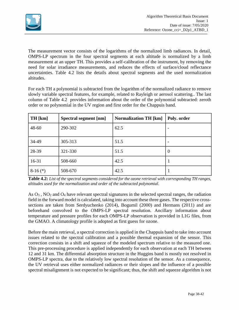
Algorithm Theoretical Basis Document
Issue: 1
Date of issue: 7/05/2020
Reference: Ozone_cci+_D2p1_ATBD_1
Page 38-42
The measurement vector consists of the logarithms of the normalized limb radiances. In detail,
OMPS-LP spectrum in the four spectral segments at each altitude is normalized by a limb
measurement at an upper TH. This provides a self-calibration of the instrument, by removing the
need for solar irradiance measurements, and reduces the effects of surface/cloud reflectance
uncertainties. Table 4.2 lists the details about spectral segments and the used normalization
altitudes.
For each TH a polynomial is subtracted from the logarithm of the normalized radiance to remove
slowly variable spectral features, for example, related to Rayleigh or aerosol scattering.. The last
column of Table 4.2 provides information about the order of the polynomial subtracted: zeroth
order or no polynomial in the UV region and first order for the Chappuis band.
TH [km] Spectral segment [nm] Normalization TH [km] Poly. order
48-60 290-302 62.5 -
34-49 305-313 51.5 -
28-39 321-330 51.5 0
16-31 508-660 42.5 1
8-16 (*) 508-670 42.5 1
Table 4.2: List of the spectral segments considered for the ozone retrieval with corresponding TH ranges,
altitudes used for the normalization and order of the subtracted polynomial.
As O3 , NO2 and O4 have relevant spectral signatures in the selected spectral ranges, the radiation
field in the forward model is calculated, taking into account these three gases. The respective cross-
sections are taken from Serdyuchenko (2014), Bogumil (2000) and Hermans (2011) and are
beforehand convolved to the OMPS-LP spectral resolution. Ancillary information about
temperature and pressure profiles for each OMPS-LP observation is provided in L1G files, from
the GMAO. A climatology profile is adopted as first guess for ozone.
Before the main retrieval, a spectral correction is applied in the Chappuis band to take into account
issues related to the spectral calibration and a possible thermal expansion of the sensor. This
correction consists in a shift and squeeze of the modeled spectrum relative to the measured one.
This pre-processing procedure is applied independently for each observation at each TH between
12 and 31 km. The differential absorption structure in the Huggins band is mostly not resolved in
OMPS-LP spectra, due to the relatively low spectral resolution of the sensor. As a consequence,
the UV retrieval uses either normalized radiances or their slopes and the influence of a possible
spectral misalignment is not expected to be significant; thus, the shift and squeeze algorithm is not
Algorithm Theoretical Basis Document
Issue: 1
Date of issue: 7/05/2020
Reference: Ozone_cci+_D2p1_ATBD_1
Page 39-42
applied. Typical values of the spectral shift are inside the range [+1,+4] nm for the first point of
the interval and [-2,+1] nm for the last spectral point.
For all spectral ranges, the measurement noise covariance matrix is obtained at this stage from the
fit residuals, after all the relevant gases in the selected spectral windows have been fitted. The
noise to signal ratio is taken as the root mean square of the fit residuals and fed into SCIATRAN.
Surface albedo is retrieved simultaneously, by assuming a Lambertian surface and using the sun-
normalized radiance. For the albedo retrieval, we selected two spectral ranges at TH around 38
km: 350-365 nm and 445-455 nm, where ozone absorption is weak.
4.2.3 OMPS-LP Usask retrieval algorithm
4.3 SAGE-CCI-OMPS Extension (FMI)
The merged monthly zonal mean dataset of ozone profiles, which is also referred to as the SAGE-
CCI-OMPS dataset, is created using the data from several satellite instruments: SAGE II on ERBS,
GOMOS, SCIAMACHY and MIPAS on Envisat, OSIRIS on Odin, ACE-FTS on SCISAT, and
OMPS on Suomi-NPP. This dataset has been created in the framework of Ozone_cci project
(Sofieva et al., 2017). Originally, the datasets covered the time period from 1984 to 2016, but now
it is regularly extended.
The stability of the individual-instrument data records has been extensively studied; only stable
data are used for the merged dataset.
All the data used for creating the merged dataset have a sufficiently good resolution of 2–3 km in
the UTLS. For all instruments, ozone profiles are retrieved on the geometric altitude grid. The
majority of the datasets -SAGE II, GOMOS, OSIRIS, SCIAMACHY and OMPS - provide number
density ozone profiles; therefore this representation is used for the merged dataset. For ACE-FTS
and MIPAS, the retrievals are in volume mixing ratio on altitude grid. Conversion to number
density profiles is performed using temperature profiles retrieved by these instruments, thus
providing consistent (i.e., without using external information about temperature and pressure
profiles) representation of number density ozone profiles.
The information about individual datasets is collected in Table 4.3.1. For some instruments, the
selected time period is shorter than the full operation period. The individual datasets have been
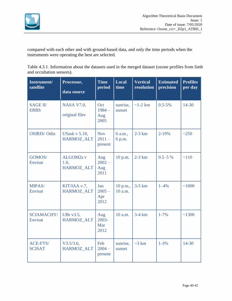
Algorithm Theoretical Basis Document
Issue: 1
Date of issue: 7/05/2020
Reference: Ozone_cci+_D2p1_ATBD_1
Page 40-42
compared with each other and with ground-based data, and only the time periods when the
instruments were operating the best are selected.
Table 4.3.1. Information about the datasets used in the merged dataset (ozone profiles from limb
and occultation sensors).
Instrument/
satellite
Processor,
data source
Time
period
Local
time
Vertical
resolution
Estimated
precision
Profiles
per day
SAGE II/
ERBS
NASA V7.0,
original files
Oct
1984 –
Aug
2005
sunrise,
sunset
~1-2 km 0.5-5% 14-30
OSIRIS/ Odin USask v 5.10,
HARMOZ_ALT
Nov
2011 –
present
6 a.m.,
6 p.m.
2-3 km 2-10% ~250
GOMOS/
Envisat
ALGOM2s v
1.0,
HARMOZ_ALT
Aug
2002 –
Aug
2011
10 p.m. 2-3 km 0.5–5 % ~110
MIPAS/
Envisat
KIT/IAA v.7,
HARMOZ_ALT
Jan
2005 –
Apr
2012
10 p.m.,
10 a.m.
3-5 km 1–4% ~1000
SCIAMACHY/
Envisat
UBr v3.5,
HARMOZ_ALT
Aug
2003-
Mar
2012
10 a.m. 3-4 km 1-7% ~1300
ACE-FTS/
SCISAT
V3.5/3.6,
HARMOZ_ALT
Feb
2004 –
present
sunrise,
sunset
~3 km 1-3% 14-30

Algorithm Theoretical Basis Document
Issue: 1
Date of issue: 7/05/2020
Reference: Ozone_cci+_D2p1_ATBD_1
Page 41-42
OMPS/ Suomi
NPP
USask 2D,
HARMOZ_ALT
Apr
2012-
present
1:30
p.m.
~2 km 2-10% ~1600
The merged dataset is created in 10° latitude zones from 90°S to 90°N, in the altitude range 10 –
50 km.
The merging is performed on the deseasonalized anomalies computed from each individual
dataset. The details of the merging procedure can be found in (Sofieva et al., 2017).
The main dataset consists of the merged deseasonalized anomalies and their uncertainties. For the
purpose of other applications (e.g., comparisons with models etc.), we presented the ozone profile
also in number density. The computing of merged number density profiles from the merged
deseasonalized anomalies is performed via restoring the seasonal cycle in the data. The best
estimate of the amplitude of seasonal cycle is given by MIPAS measurements, because they
provide all season pole-to-pole measurements with dense sampling. We take the absolute values
of the seasonal cycle from SAGE II and OSIRIS in the overlapping period (which are very close
to each other and also with GOMOS measurements), thus preserving the consistency in the dataset
through the whole observation period.
The merged SAGE-CCI_OMPS is actively used in ozone trends analyses and in ozone assessments
(WMO 2014. 2018; Petropavlovskikh et al., 2019; Weber et al., 2018, 2019).

Algorithm Theoretical Basis Document
Issue: 1
Date of issue: 7/05/2020
Reference: Ozone_cci+_D2p1_ATBD_1
Page 42-42
4.4 Gridded merged Level 3 dataset (FMI) The merged gridded dataset of ozone profiles is significantly developed further in the Ozone CCI+
project. The monthly zonal mean gridded ozone profile dataset is provided in the altitude range
from 10 km to 50 km. It covers the time period from late 2001 until now. The data are gridded
monthly in the 10° latitude x 20° longitude zones. Since the sampling of solar occultation
measurements is rather low, they are not included. The gridded ozone profiles are computed first
separately for GOMOS, MIPAS, SCIAMACHY, OSIRIS, OMPS-LP, MLS, and they are also
merged into one dataset. The information about the individual datasets can be found Tables 4.1
and 4.3. The principle of creating the Level 3 gridded data for individual datasets, as well as data
merging is the same as for the monthly zonal mean dataset.