Embed Size (px)
Citation preview
`p-Norm Multiple Kernel LearningMaking Learning with Multiple Kernels Effective

`p-Norm Multiple Kernel Learning
vorgelegt von Dipl.-Math.
Marius Kloft
Von der Fakultat IV - Elektrotechnik und Informatikder Technischen Universitat Berlin zur Erlangung des akademischen Grades
Doktor der Naturwissenschaften– Dr. rer. nat. –
genehmigte
Dissertation
Promotionsausschuss:
Vorsitzender: Prof. Dr. Manfred Opper
Fakultat IV – Elektrotechnik und Informatik
Technische Universitat Berlin
Berichter: Prof. Dr. Klaus-Robert MullerFakultat IV – Elektrotechnik und Informatik
Technische Universitat Berlin
Prof. Dr. Peter L. BartlettDepartment of EECS and Department of Statistics
University of California, Berkeley, USA
Prof. Dr. Gilles BlanchardInstitut fur Mathematik
Universitat Potsdam
Tag der mundlichen Aussprache: 26.09.2011
Berlin, 2011D 83

To my parents
Acknowledgements
I am deeply grateful for the opportunity to have worked with so many brilliant andcreative minds over the last years. First of all, I would like to thank my PhD advisorsProf. Dr. Klaus-Robert Muller, Prof. Dr. Peter L. Bartlett, and Prof. Dr. GillesBlanchard. Of course, I owe the utmost gratitude to Professor Muller, who initiallyintroduced me to the subject of machine learning in 2007; with his infectious optimism,wit, and curiosity, he created the open and stimulating atmosphere that characterizeshis Machine Learning Laboratory at TU Berlin. It was also Professor Muller who gaveme advice and support in various respects from the very beginning of my PhD studies,thus turning out to be much more than just a scientific advisor. I am deeply thankfulto him. By the same token, I would like to thank all members of his lab for creatingsuch a pleasurable working atmosphere in the office each day, most notably my formerand current office mates Pascal Lehwark, Nico Gornitz, Gregoire Montavon, and StefanHaufe.
Furthermore, I would like to thank Professor Bartlett very much indeed for kindlyinviting me over to visit his learning theory group at UC Berkeley, a most enjoyable andinspiring experience in many ways, and, most of all, for introducing me to the fascinat-ing world of learning theory; his readiness to share his vast knowledge with me allowedme to gain a deeper understanding of the field. I also thank all members of his group,especially Alekh, for our stimulating discussions, not limited tovarious mathematical subjects, but also in matters of the every-day life. I also thank all office mates in Sutardja Dai Hall forthe nice atmosphere, and the UC Berkeley for providing such agreat office with an absolutely stunning view of the SF Bay, all ofwhich contributed to making my stay (Oct 2009–Sep 2010) sucha memorable one.
Likewise, I am very grateful to Professor Blanchard for taking so much of his valu-able time for our extensive and fruitful discussions on various mathematical problems,sharing his immense knowledge and deep insights with me. I remember us sitting incafes for hours, trying to solve a mathematical puzzle arising from our joint research
III
projects. It is rare that a professor invests so much of his time in mentoring a studentand I owe him a big thanks!
My special thanks go to Dr. Ulf Brefeld for his caring mentoring and patientteaching in the initial phase of my PhD, which considerably eased the start. Hisencouragement gave me strength and confidence. Likewise, I thank Dr. Ulrich Ruckertfor his mentoring while both of us were with the UC Berkeley, which substantially spedup my introduction to learning theory. Moreover, I am indebted to Dr. AlexanderZien for countless stimulating discussions and to Dr. Soren Sonnenburg and AlexanderBinder for sharing their great insights in the SHOGUN toolbox with me. Furthermore,I would like to thank all members of the REMIND project team, especially Dr. KonradRieck and Dr. Pavel Laskov, for the warm and nice atmosphere that made working inthe team (2007–2009) such an effective and also fun experience.
I especially thank Claudia for so carefully proof-reading my manuscript in the finalstage with respect to grammar and spelling, and Helen, who suffered the most from myobsession with unfinished chapters and last-minute changes to the manuscript, for herpatience and support. Most of all, I would like to thank my parents for supporting mein every conceivable way.
Finally, I acknowledge financial support of the German Bundesministerium furBildung und Forschung (BMBF), under the project REMIND (FKZ 01-IS07007A), andthe European Community, under the PASCAL2 Network of Excellence of the FP7-ICTprogram (ICT-216886). I acknowledge the Berlin Institute of Technology (TU Berlin)and the German Academic Exchange Service (DAAD) for PhD student scholarships of1-year runtime each.
IV
Abstract
The goal of machine learning is to learn unknown concepts from data. In real-worldapplications such as bioinformatics and computer vision, data frequently arises frommultiple heterogeneous sources or is represented by various complementary views, theright choice—or even combination—of which being unknown. To this end, the multiplekernel learning (MKL) framework provides a mathematically sound solution. Previousapproaches to learning with multiple kernels promote sparse kernel combinations tosupport interpretability and scalability. Unfortunately, classical approaches to learningwith multiple kernels are rarely observed to outperform trivial baselines in practicalapplications.
In this thesis, I approach learning with multiple kernels from a unifying view whichshows previous works to be only particular instances of a much more general familyof multi-kernel methods. To allow for more effective kernel mixtures, I have developedthe `p-norm multiple kernel learning methodology, which, to sum it up, is both moreefficient and more accurate than previous approaches to multiple kernel learning, asdemonstrated on several data sets. In particular, I derive optimization algorithms thatare much faster than the commonly used ones, allowing to deal with up to ten thousandsof data points and thousands of kernels at the same time. Empirical applications of`p-norm MKL to diverse, challenging problems from the domains of bioinformatics andcomputer vision show that `p-norm MKL achieves accuracies that surpass the state-of-the-art.
The proposed techniques are underpinned by deep foundations in the theory oflearning: I prove tight lower and upper bounds on the local and global Rademachercomplexities of the hypothesis class associated with `p-norm MKL, which yields excessrisk bounds with fast convergence rates, thus being tighter than existing bounds forMKL, which only achieve slow convergence rates. I also connect the minimal values ofthe bounds with the soft sparsity of the underlying Bayes hypothesis, proving that fora large range of learning scenarios `p-norm MKL attains substantial stronger general-ization guarantees than classical approaches to learning with multiple kernels. Using amethodology based on the theoretical bounds, and exemplified by means of a controlledtoy experiment, I investigate why MKL is effective in real applications.
Data sets, source code and implementations of the algorithms, additional scriptsfor model selection, and further information are freely available online.
V

Zusammenfassung
Ziel des Maschinellen Lernens ist das Erlernen unbekannter Konzepte aus Daten. Invielen aktuellen Anwendungsbereichen des Maschinellen Lernens, wie zum Beispiel derBioinformatik oder der Computer Vision, sind die Daten auf vielfaltige Art und Weisein Merkmalsgruppierungen reprasentiert. Im Voraus ist allerdings die optimale Kom-bination jener Merkmalsgruppen oftmals unbekannt. Die Methodologie des Lernensmit mehreren Kernen bietet einen attraktiven und mathematisch fundierten Ansatz zudiesem Problem. Existierende Modelle konzentrieren sich auf dunn besetzte Merkmals-bzw. Kernkombinationen, um deren Interpretierbarkeit zu erleichtern. Allerdings er-weisen sich solche klassischen Ansatze zum Lernen mit mehreren Kernen in der Praxisals wenig effektiv.
In der vorliegenden Dissertation betrachte ich das Problem des Lernens mit meh-reren Kernen aus einer neuartigen, generelleren Perspektive. In dieser Sichtweise sindklassische Ansatze nur Spezialfalle eines wesentlich generelleren Systems des Lernensmit mehreren Kernen. Um effektivere Kernmischungen zu erhalten, entwickle ich die`p-norm multiple kernel learning Methodologie, die sich effizienter und effektiver alsvorherige Losungsansatze erweist. Insbesondere leite ich Algorithmen zur Optimierungdes Problems her, die wesentlich schneller sind als existierende und es erlauben, gle-ichzeitig Zehntausende von Trainingsbeispielen und Tausende von Kernen zu verar-beiten. Ich analysiere die Effektivitat unserer Methodologie in einer Vielzahl vonschwierigen und hochzentralen Problemen aus den Bereichen Bioinformatik und Com-puter Vision und zeige, dass `p-norm multiple kernel learning Vorhersagegenauigkeitenerreicht, die den neuesten Stand der Forschung ubertreffen.
Die entwickelten Techniken sind tief untermauert in der Theorie des MaschinellenLernens: Ich beweise untere und obere Schranken auf die Komplexitat der zugehorigenHypothesenklasse, was die Herleitung von Generalisierungsschranken erlaubt, die eineschnellere Konvergenzgeschwindigkeit haben als vorherige Schranken. Des Weiterenstelle ich den minimalen Wert der Schranken mit den geometrischen Eigenschaften derBayes-Hypothese in Verbindung. Darauf basierend beweise ich, dass fur eine große An-zahl von Szenarien `p-norm multiple kernel learning deutlich starkere Generalisierungs-garantien aufweist als vorherige Ansatze zum Lernen mit mehreren Kernen. Mit Hilfeeiner von mir vorgeschlagenen Methodik, basierend auf den theoretischen Schrankenund sogenannten kernel alignments, untersuche ich, warum sich `p-norm multiple ker-nel learning als hocheffektiv in praktischen Anwendungsgebieten erweist.
Die eingesetzten Datensatze, der Quellcode und die Implementierungen der Algo-rithmen sowie weitere Informationen zur Benutzung sind online frei verfugbar.
VII

Contents
I Introduction and Overview 1I Introduction and Overview 3
1 Introduction . . . . . . . . . . . . . . . . . . . . . . . . . . . . . . . . 3
1.1 Author’s PhD Thesis . . . . . . . . . . . . . . . . . . . . . . . . . 4
1.2 Organization of this Dissertation and Own Contributions . . . . 4
1.3 Multiple Kernel Learning in a Nutshell . . . . . . . . . . . . . . . 8
1.4 Basic Notation . . . . . . . . . . . . . . . . . . . . . . . . . . . . 12
2 A Unifying View of Multiple Kernel Learning . . . . . . . . . . . 13
2.1 A Regularized Risk Minimization Approach . . . . . . . . . . . . 13
2.2 Dual Problem . . . . . . . . . . . . . . . . . . . . . . . . . . . . . 15
2.3 Recovering Prevalent MKL Formulations as Special Cases . . . . 16
2.4 Summary and Discussion . . . . . . . . . . . . . . . . . . . . . . 20
II `p-norm Multiple Kernel Learning 23II `p-norm Multiple Kernel Learning 25
3 Algorithms . . . . . . . . . . . . . . . . . . . . . . . . . . . . . . . . . 31
3.1 Block Coordinate Descent Algorithm . . . . . . . . . . . . . . . . 31
3.2 Large-Scale Algorithm . . . . . . . . . . . . . . . . . . . . . . . . 33
3.3 Implementation . . . . . . . . . . . . . . . . . . . . . . . . . . . . 37
3.4 Runtime Experiments . . . . . . . . . . . . . . . . . . . . . . . . 40
3.5 Summary and Discussion . . . . . . . . . . . . . . . . . . . . . . 43
4 Theoretical Analysis . . . . . . . . . . . . . . . . . . . . . . . . . . . 45
4.1 Global Rademacher Complexity . . . . . . . . . . . . . . . . . . . 46
4.2 Local Rademacher Complexity . . . . . . . . . . . . . . . . . . . 49
4.3 Excess Risk Bounds . . . . . . . . . . . . . . . . . . . . . . . . . 61
4.4 Why Can Learning Kernels Help Performance? . . . . . . . . . . 67
4.5 Summary and Discussion . . . . . . . . . . . . . . . . . . . . . . 70
5 Empirical Analysis and Applications . . . . . . . . . . . . . . . . . 71
5.1 Goal and Experimental Methodology . . . . . . . . . . . . . . . . 71
5.2 Case Study 1: Toy Experiment . . . . . . . . . . . . . . . . . . . 74
IX
Contents
5.3 Case Study 2: Real-World Experiment (TSS) . . . . . . . . . . . 78
5.4 Bioinformatics Experiments . . . . . . . . . . . . . . . . . . . . . 82
5.5 Computer Vision Experiment . . . . . . . . . . . . . . . . . . . . 92
5.6 Summary and Discussion . . . . . . . . . . . . . . . . . . . . . . 97
Conclusion and Outlook 101
Appendix 105
A Foundations . . . . . . . . . . . . . . . . . . . . . . . . . . . . . . . . . 105
A.1 Why Using Kernels? . . . . . . . . . . . . . . . . . . . . . . . . . 105
A.2 Basic Learning Theory . . . . . . . . . . . . . . . . . . . . . . . . 107
A.3 Convex Optimization . . . . . . . . . . . . . . . . . . . . . . . . 110
B Relating Tikhonov and Ivanov Regularization . . . . . . . . . . . 111
C Supplements to the Theoretical Analysis . . . . . . . . . . . . . . 112
D Cutting Plane Algorithm . . . . . . . . . . . . . . . . . . . . . . . . 115
Bibliography 121
Curriculum Vitae 131
Publications 133
X

Part I
Introduction and Overview
1

I Introduction and Overview
1 Introduction
The goal of machine learning is to learn unknown concepts from data. But the success ofa learning machine crucially depends on the quality of the data representation. At thispoint, the paradigm of kernel-based learning (Scholkopf et al., 1998; Muller et al., 2001)offers an elegant way for decoupling the learning and data representation processes ina modular fashion. This allows to obtain complex learning machines from simple linearones in a canonical way. Nowadays, kernel machines are frequently employed in modernapplication domains that are characterized by vast amounts of data along with highlynon-trivial learning tasks such as bioinformatics or computer vision, for their favorablegeneralization performance while maintaining computational feasibility.
However, after more than a decade of research it still remains an unsolved problemto find the best kernel for a task at hand. Most frequently, the kernel is selectedfrom a candidate set according to its generalization performance on a validation set,which is held back at training time. Clearly, the performance of such an algorithm islimited by the performance of the best kernel in the set and can be arbitrarily bad ifthe kernel does not match the underlying learning task. Unfortunately, in the currentstate of research, there is little hope that in the near future a machine will be ableto automatically engineer the perfect kernel for a particular problem at hand (Searle,1980). However, by restricting ourselves to a less general problem, can we legitimatelyhope to obtain a mathematically sound solution? And if so, which restrictions have tobe imposed?
A first step towards a more realistic model of learning the kernel was achievedin Lanckriet et al. (2004a), who showed that, given a candidate set of kernels, it iscomputationally feasible to simultaneously learn a support vector machine and a linearkernel combination at the same time, if the so-formed kernel combinations are requiredto be positive-definite and trace-norm normalized. This framework was entitled mul-tiple kernel learning (MKL). Research in the following years focused on speeding upthe initially demanding optimization algorithms (e.g. Sonnenburg et al., 2006a; Rako-tomamonjy et al., 2008)—ignoring the fact that empirical evidence for the superiorityof learning with multiple kernels over single-kernel baselines was missing.
By imposing an `1-norm regularizer on the kernel weights, classical approaches tomultiple kernel learning promote sparse kernel combinations to support interpretabilityand scalability. Unfortunately, sparseness is not always beneficial and can be restrictivein practice, for example, in the presence of complementary kernel sets. However, nega-
3
I Introduction and Overview
tive results are less often published in science than positive ones. It took until 2008 forconcerns regarding the effectiveness of multiple kernel learning in practical applicationsto be raised, starting in the domains of bioinformatics (Noble, 2008) and computervision (Gehler and Nowozin, 2008): a multitude of researchers presented empirical evi-dence showing that, in practice, multiple kernel learning is frequently outperformed bya simple uniform kernel combination (Cortes et al., 2008, 2009a; Gehler and Nowozin,2009; Yu et al., 2010). The whole discussion peaked in the provocative question “Canlearning kernels help performance?” posed by Corinna Cortes in an invited talk atICML 2009 (Cortes, 2009).
Consequently, despite all the substantial progress in the field of multiple kernellearning, there still remains an unsatisfied need for an approach that is really useful forpractical applications: a model that has a good chance of improving the accuracy (overa plain sum kernel) together with an implementation that matches today’s standards(i.e., that can be trained on 10,000s of data points in a reasonable time). Even worse,despite the recent attempts for clarification (Lanckriet et al., 2009), underlying reasonsfor the empirical picture remain unclear. At this point, I argue that all of this is nowachievable, thus answering Corinna Cortes’s research question in the affirmative:
1.1 Author’s PhD Thesis
This dissertation concerns the validation of the following thesis:
`p-norm multiple kernel learning, a methodology that I developed and ofwhich I show that it enjoys favorable theoretical guarantees, is both fasterand more accurate than existing approaches to learning with multiple ker-nels, finally making multiple kernel learning effective in practical applica-tions.
1.2 Organization of this Dissertation and Own Contributions
Part I: Introduction and Overview
I start my dissertation in Chapter 1 with a short introduction to and motivation ofmultiple kernel learning (MKL), containing, in a nutshell, the statement of the problemto be solved and examples of practical applications where it arises, taken from thedomains of bioinformatics and computer vision.
In Chapter 2, I formally introduce a rigorous mathematical view of the prob-lem, deferring mathematical preliminaries to Appendix A. Deviating from standardintroductions, I phrase MKL as a general optimization criterion based on structuredregularization, covering and also unifying existing formulations under a common um-brella; from this point of view, classical MKL is only a particular instance of a moregeneral family of MKL methods. This allows to analyze a large variety of MKL meth-ods jointly, as exemplified by deriving a general dual representation of the criterion,
4
1 Introduction
without making assumptions on the employed norm or the loss, beside being convex.This not only delivers insights into connections between existing MKL formulations,but also allows to derive new ones as special cases of the unifying view.
Previously Published Work
This thesis is based on the following selected publications.
The core framework was published in:
[1] M. Kloft, U. Brefeld, P. Laskov, and S. Sonnenburg. Non-sparse multiple kernellearning. In Proc. of the NIPS 2008 Workshop on Kernel Learning: AutomaticSelection of Kernels, 2008.
[2] M. Kloft, U. Brefeld, S. Sonnenburg, P. Laskov, K.-R. Muller, and A. Zien.Efficient and accurate lp-norm multiple kernel learning. In Advances in Neural Infor-mation Processing Systems 22 (NIPS 2009), pages 997–1005. MIT Press, 2009.
[3] M. Kloft, U. Brefeld, S. Sonnenburg, and A. Zien. Lp-norm multiple kernellearning. Journal of Machine Learning Research (JMLR), 12:953–997, 2011.
The main idea of `p-norm MKL was initially presented in [1]. The core framework wassubsequently published in [2]-[3].
Theoretical aspects were presented in:
[4] M. Kloft, U. Ruckert, and P. L. Bartlett. A unifying view of multiple kernellearning. In Proceedings of the European Conference on Machine Learning (ECML),2010.
[5] M. Kloft and G. Blanchard. The local Rademacher Complexity of Multiple KernelLearning. ArXiv preprint 1103.0790v1, 2011. Short version submitted to NIPS 2011,Jun 2011. Full version submitted to Journal of Machine Learning Research (JMLR),Mar 2011.
Applications to computer vision were discussed in:
[6] A. Binder, S. Nakajima, M. Kloft, C. Muller, W. Wojcikiewicz, U. Brefeld, K.-R.Muller, and M. Kawanabe. Classifying Visual Objects with Multiple Kernels. Submit-ted to IEEE Transactions on Pattern Analysis and Machine Intelligence (TPAMI). Apreliminary version is published in Proceedings of the 12th Workshop on Information-based Induction Sciences, 2010.
The content of this thesis is related to the above publications in the following way. Chapter 2is based on [4]; Chapter 3 is based on [1]-[3]; Chapter 4 is based on [5]; Chapter 5 containsmaterial from [1]-[3] and [6].
Note: a complete list of all publications is shown at the end of the bibliographysection.
5
I Introduction and Overview
Part II: `p-norm Multiple Kernel Learning
In the main part of my dissertation, I introduce a novel instantiation of the proposedgeneral criterion, which I entitle `p-norm multiple kernel learning. Recognizing classicalapproaches to learning with multiple kernels as the special case of deploying `1-normand hinge loss, I argue that, from the structured point of view, it is more natural to chosean intermediate norm rather than an extreme `1-norm. I show the general connection ofthe structured formulation to the learning-kernels formulation that is usually consideredin the literature. For classical MKL, this connection is known from the seminal paperof Bach et al. (2004); here, I show that it applies to a whole family of MKL algorithms,no matter which convex loss function or structured `p-norm regularizer is employed.The remainder of my dissertation focuses on the analysis of `p-norm MKL in terms ofoptimization algorithms, theoretical justification, empirical analysis, and applicationsto bioinformatics and computer vision.
Chapter 3 is on optimization algorithms. Considering the gain in prediction accu-racy achieved by `p-norm MKL, established later in this dissertation, one might expecta substantial drawback with respect to execution time—the contrary is the case: thepresented algorithms allow us to deal with ten thousands of data points and thousandsof kernels at the same time, being up to two magnitudes faster than the state-of-the-art in MKL research, including HessianMKL and SimpleMKL. Some of these, like thecutting-plane strategy, which was designed by me and implemented with the help ofSoren Sonnenburg and Alexander Zien, are based on previous work by Sonnenburget al. (2006a), others like the analytical solver are completely novel. The latter one isbased on a simple analytical formula that can be evaluated in micro seconds, and thus,despite its efficiency, is even simpler than SimpleMKL, which requires a heuristic linesearch. I show it being provably convergent, using the usual regularity assumptions. Ialso wrote macro scripts, completely automating the whole process from training overmodel selection to evaluation. Currently, MKL can be trained and validated by a singleline of code including random subsampling, model search for the optimal parametersC and p, and collection of results.1
In Chapter 4, the proposed techniques are justified from a theoretical point of view.I prove tight lower and upper bounds on the local and global Rademacher complexitiesof the hypothesis class associated with `p-norm MKL, which yields excess risk boundswith fast convergence rates, thus being tighter than existing bounds for MKL, whichonly achieved slow convergence rates. For the results on the local complexities to hold,I find an assumption on the uncorrelatedness of the kernels; a similar assumption wasalso recently used by Raskutti et al. (2010), but in the different context of sparse re-covery.
Even the tightest previous theoretical analyses such as the one carried out by Corteset al. (2010a) for the special case of classical MKL were not able to answer the researchquestion “Can learning kernels help performance?” (Cortes, 2009). In contrast, beside
1Implementation freely available under the GPL license at http://doc.ml.tu-berlin.de/nonsparse_mkl/.
6
1 Introduction
reporting on the worst-case bounds, I also connect the minimal values of the theoreticalbounds with the geometry of the underlying learning scenario (namely, the soft spar-sity of the Bayes hypothesis), in particular, proving that for a large range of learningscenarios `p-norm MKL attains a strictly “better” (i.e., lower) bound than classical`1-norm MKL and the SVM using a uniform kernel combination. This theoreticallyjustifies using `p-norm MKL and multiple kernel learning in general.
Chapter 5 concerns the empirical analysis of `p-norm MKL and applications todiverse, challenging problems from the domains of bioinformatics and computer vision.From a practical point of view, this is the most important chapter of my dissertation asI show here that `p-norm MKL works well in practice. For the experiments, problemsfrom the domains of bioinformatics and computer vision were chosen, not only becausethey come with highly topical, challenging, small- and large-scale prediction tasks, butalso because researchers frequently encounter multiple kernels or data sources here.This renders these domains especially appealing for the use of MKL.
At this point, it has to be admitted that other researchers also deployed MKL to thosedomains: Lanckriet et al. (2004b) experimented on bioinformatics data and Varma andRay (2007) and Gehler and Nowozin (2009) on computer vision data. However, noneof those studies were able to prove the practical effectiveness of MKL. The first studyinvestigated whether MKL can help performance in genomic data fusion: indeed, MKLoutperformed the best single-kernel SVM as determined by model selection; however,the uniform kernel combination was not investigated at that point. Subsequent inves-tigations showed here that the latter outperforms MKL on the very same data set.2
In the second study, MKL was shown to substantially outperform the uniform kernelcombination on the caltech-101 object recogniction data set. This study turned out tobe incorrect due to a flaw in the kernel generation.3 Subsequently, MKL was studiedon the very same data set by Gehler and Nowozin (2009) and found to be outperformedby an SVM using a uniform kernel combination. To the best of my knowledge, theonly confirmed experiment concerning MKL outperforming the SVM using a uniformkernel combination is the one undertaken by Zien and Ong (2007) in the context ofprotein subcellular localization prediction.
In this thesis, I show that by considering `p-norms, MKL can in fact help performancein both of the above applications (genomic data fusion and object recognition). Besides,I study applications to gene transcription start site detection, protein fold prediction,and metabolic network reconstruction. While I observe that MKL helps performancein some applications (including the ones mentioned in the above paragraph, where re-searchers tried for years making MKL effective), I also show that sometimes MKL doesnot increase the performance (this is, for example, the case for the metabolic networkreconstruction experiment). The raises the question why it sometimes helps and whysometimes it does not. At this point, I introduce a methodology deploying both, the
2Personal correspondences with William S. Noble; see W. Noble’s talk at http://videolectures.
net/lkasok08_whistler/, June 20, 2011.3See errata on the first author’s personal homepage, http://research.microsoft.com/en-us/um/
people/manik/projects/trade-off/caltech101.html, June 20, 2011.
7
I Introduction and Overview
bounds that I prove in the theoretical chapter of this thesis and the kernel alignmenttechniques initially proposed in a different context by Cristianini et al. (2002). Whilethe theoretical bounds are used to investigate the optimal norm parameter p, showingthat the effectiveness of MKL is connected with the soft sparsity of the underlyingBayes hypothesis, the alignments are used to study whether the kernels at hand arecomplementary or rather redundant. The whole methodology is exemplified by meansof a toy experiment, where I artificially construct the Bayes hypothesis, controllingthe underlying soft sparsity of the problem. It is shown that MKL’s empirical per-formance can crucially depend on the choice of the norm parameter p and that theoptimality of such a parameter can highly depend on the geometry of the underlyingBayes hypothesis (it can make the difference between 4% or 43% test error, as shownin the simulations). The chapter concludes with my study, carried out with the helpof Shinichi Nakajima, on object recogniction, the very same application unsuccessfullystudied earlier by Varma and Ray (2007) and Gehler and Nowozin (2009)—see dis-cussion above—where classical MKL could not help performance. In contrast, I showthat, by deploying the proposed `p-norm multiple kernel learning and taking p = 1.11in median, the prediction accuracy can be raised over the SVM baselines, regardless ofthe class, by an AP score of 1.5 in average, and for 7 out of the 20 classes significantlyso, concluding the final Chapter 5 of my thesis.
1.3 Multiple Kernel Learning in a Nutshell
In this section, we introduce the problem of multiple kernel learning.
Problem setting In classical supervised machine learning we are given training exam-ples x1, . . . , xn lying in some input space X and labels y1, . . . , yn ∈ Y, in the simplestcase, X = Rd and Y = −1, 1. The goal in supervised learning is to find a predic-tion function f : X → Y from a given set H ⊂ YX that has a low error rate on newdata
(xn+1, yn+1
), . . . ,
(xn+l, yn+l
)stemming from the same data source but which is
unseen at training time. Clearly, we cannot learn anything useful at all if the trainingdata and the new data are not connected in any way. Therefore one usually assumes astochastic mechanism underlying the data generation process, most commonly, that allof the
(xi, yi
)are drawn independently from one and the same probability distribution
P . In this case the quality of the prediction function f is measured by the expectedrate of false predictions E(x,y)∼P1f(x)6=y.
Regularized risk minimization An often-employed approach to this problem is regu-larized risk minimization (RRM), where a minimizer
f∗ ∈ argminf∈H Ω(f) + CLn(f)
is found. Hereby Ln(f) =∑n
i=1 l (f(xi), yi) is the (cumulative) empirical loss of ahypothesis f with respect to a function l : R×Y → R (called loss function) that upperbounds the 0-1 loss 1f(x) 6=y and Ω : H → R is a mapping (called regularizer). Thename risk minimization stems from the fact that Ln is n-times the empirical risk. Wecan interpret RRM as minimizing a trade-off between the empirical loss (to classify the
8
1 Introduction
training data well) and a regularizer (to penalize the complexity of f and thus avoidoverfitting), where the trade-off is controlled by a positive parameter C.
Kernel methods Single-kernel approaches to RRM (Vapnik, 1998) simply use linearmodels of the form fw,b(x) = 〈w, x〉+ b but—this is the core idea of kernel methods—replace all resulting inner products 〈x, x〉 by so-called kernels k(x, x). Roughly speak-ing, a kernel k is a clever way to efficiently compute inner products in a possibly veryhigh-dimensional feature space. As outlined in the introduction, the ultimate goal ofkernel learning would be to find the best kernel for a problem at hand—but this is atask too hard to allow for a general solution so that, in practice, the kernel is usuallyeither fixed a priori or selected from a small candidate set k1, . . . , kM according toits prediction error on a validation set, which is held back at training time.
Multiple kernel learning A first step towards finding an optimal kernel is multiplekernel learning. Here, instead of just picking a kernel from a set, a new kernel k isconstructed by combining kernels from a possibly large given set. For example, thefollowing combination rules give rise to valid kernel:
k = θ1k1 + · · ·+ θMkM (sums)
k = kθ11 · . . . · kθMM , (products)
where θ ∈ RM+ . By searching for an optimal θ, we traverse an infinitely large set of“combined kernels”. Unfortunately, except for very small M (typically M ≤ 3), thesearch space is too large to be traversed by standard methods such as grid search.
The core idea of multiple kernel learning is based on the insight that most machinelearning problems are formulated as solutions of optimization problems. What if weinclude the parameter θ as a variable into the optimization? For example, for thesupport vector machine (SVM) this task becomes
minθ≥0
SVM
( M∑m=1
θmkm
).
A first difficulty we face is that, without any further restriction on θ, the optimizationproblem may be unbounded or, for example, yield a trivial solution that does notgeneralize to new, unseen data. In the past, this has been addressed by restricting thesearch space to convex combinations (i.e., sums that add up to one). In that case theabove problem becomes (Lanckriet et al., 2004a; Bach et al., 2004)
minθ≥0, ‖θ‖1=1
SVM
( M∑m=1
θmkm
).
For quite some time, the above regularization strategy was the prevalent one in multiplekernel learning research.
`p-Norm Multiple Kernel Learning Although having been folklore among researchersfor quite a while already, it took until 2008 that criticism was made public concerning
9
I Introduction and Overview
the usefulness of the above approach in practical applications (see citations in theintroduction): it is frequently observed being outperformed by a simple, regular SVMusing a uniform kernel combination.
In this thesis, we propose to discard the restrictive convex combination requirement(which corresponds to using an `1-norm regularizer on θ) and use a more flexible `p-norm regularizer instead, leading to the optimization problem
minθ≥0, ‖θ‖p=1
SVM
( M∑m=1
θmkm
).
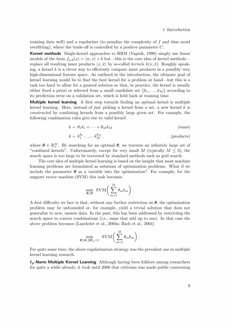
The difference between the two ways of regularizing is illustrated in the following figure,where the `1- and `2-norm regularized problems are compared. The blue line shows thenorm constraint and the green one the level sets of a quadratic function. The optimal
||x||1=1
quatric
||x||2=1
quatric
solution of the optimization problem is at-tained where the level sets of the objectivefunction touch the norm constraint. If theobjective function is convex (illustrated herefor a quadratic function), and for `1-norm thepoint of intersection is likely to be at one ofthe corners of the square (shown on the figure to the left). Because the corners arelikely to have zero-entries, sparsity is to be expected. This is in contrast to `2-normregularization, where, in general, a non-sparse solution is to be expected (shown on thefigure to the right).
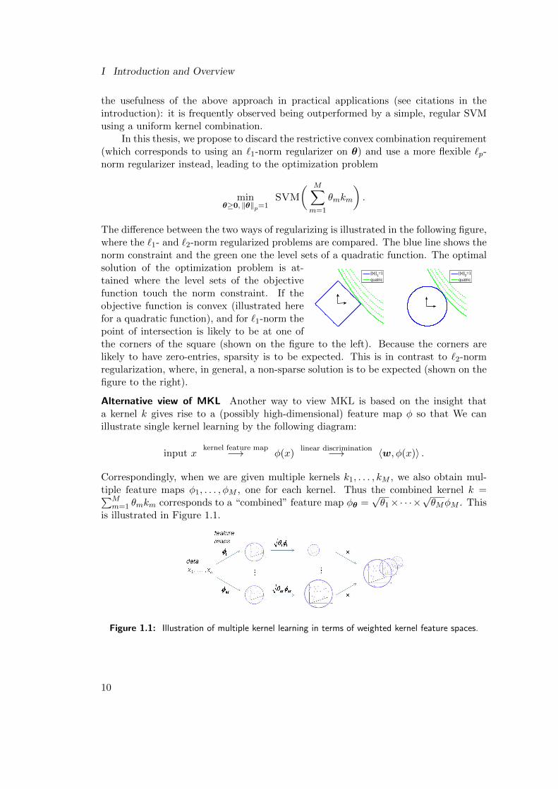
Alternative view of MKL Another way to view MKL is based on the insight thata kernel k gives rise to a (possibly high-dimensional) feature map φ so that We canillustrate single kernel learning by the following diagram:
input xkernel feature map−→ φ(x)
linear discrimination−→ 〈w, φ(x)〉 .
Correspondingly, when we are given multiple kernels k1, . . . , kM , we also obtain mul-tiple feature maps φ1, . . . , φM , one for each kernel. Thus the combined kernel k =∑M
m=1 θmkm corresponds to a “combined” feature map φθ =√θ1×· · ·×
√θMφM . This
is illustrated in Figure 1.1.
Figure 1.1: Illustration of multiple kernel learning in terms of weighted kernel feature spaces.
10
1 Introduction
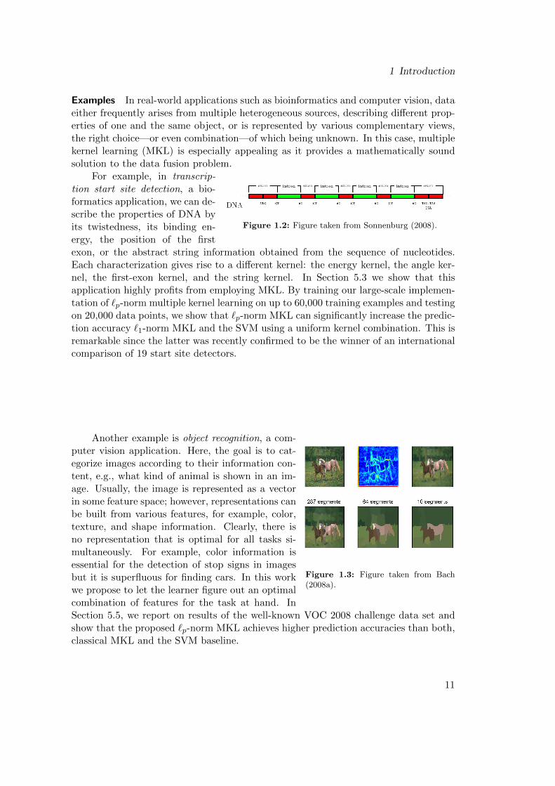
Examples In real-world applications such as bioinformatics and computer vision, dataeither frequently arises from multiple heterogeneous sources, describing different prop-erties of one and the same object, or is represented by various complementary views,the right choice—or even combination—of which being unknown. In this case, multiplekernel learning (MKL) is especially appealing as it provides a mathematically soundsolution to the data fusion problem.
Figure 1.2: Figure taken from Sonnenburg (2008).
For example, in transcrip-tion start site detection, a bio-formatics application, we can de-scribe the properties of DNA byits twistedness, its binding en-ergy, the position of the firstexon, or the abstract string information obtained from the sequence of nucleotides.Each characterization gives rise to a different kernel: the energy kernel, the angle ker-nel, the first-exon kernel, and the string kernel. In Section 5.3 we show that thisapplication highly profits from employing MKL. By training our large-scale implemen-tation of `p-norm multiple kernel learning on up to 60,000 training examples and testingon 20,000 data points, we show that `p-norm MKL can significantly increase the predic-tion accuracy `1-norm MKL and the SVM using a uniform kernel combination. This isremarkable since the latter was recently confirmed to be the winner of an internationalcomparison of 19 start site detectors.
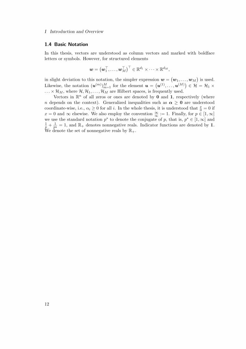
Figure 1.3: Figure taken from Bach(2008a).
Another example is object recognition, a com-puter vision application. Here, the goal is to cat-egorize images according to their information con-tent, e.g., what kind of animal is shown in an im-age. Usually, the image is represented as a vectorin some feature space; however, representations canbe built from various features, for example, color,texture, and shape information. Clearly, there isno representation that is optimal for all tasks si-multaneously. For example, color information isessential for the detection of stop signs in imagesbut it is superfluous for finding cars. In this workwe propose to let the learner figure out an optimalcombination of features for the task at hand. InSection 5.5, we report on results of the well-known VOC 2008 challenge data set andshow that the proposed `p-norm MKL achieves higher prediction accuracies than both,classical MKL and the SVM baseline.
11
I Introduction and Overview
1.4 Basic Notation
In this thesis, vectors are understood as column vectors and marked with boldfaceletters or symbols. However, for structured elements
w =(w>1 , . . . ,w
>M
)> ∈ Rd1 × · · · × RdM ,
in slight deviation to this notation, the simpler expression w =(w1, . . . ,wM
)is used.
Likewise, the notation (u(m))Mm=1 for the element u =(u(1), . . . ,u(M)
)∈ H = H1 ×
. . .×HM , where H,H1, . . . ,HM are Hilbert spaces, is frequently used.Vectors in Rn of all zeros or ones are denoted by 0 and 1, respectively (where
n depends on the context). Generalized inequalities such as α ≥ 0 are understoodcoordinate-wise, i.e., αi ≥ 0 for all i. In the whole thesis, it is understood that x
0 = 0 ifx = 0 and ∞ elsewise. We also employ the convention ∞∞ := 1. Finally, for p ∈ [1,∞]we use the standard notation p∗ to denote the conjugate of p, that is, p∗ ∈ [1,∞] and1p + 1
p∗ = 1, and R+ denotes nonnegative reals. Indicator functions are denoted by 1.We denote the set of nonnegative reals by R+.
12
2 A Unifying View of Multiple Kernel Learning
2 A Unifying View of Multiple Kernel Learning
In this chapter, we cast multiple kernel learning into a unified framework. We show thatit comprises many popular MKL variants currently discussed in the literature, includingseemingly different ones. Our approach is based on regularized risk minimization (Vap-nik, 1998). We derive generalized dual optimization problems without making specificassumptions regarding the norm or the loss function, beside that the latter is convex.Our formulation covers binary classification and regression tasks and can easily be ex-tended to multi-class classification and structural learning settings using appropriateconvex loss functions and joint kernel extensions. Prior knowledge on kernel mixturesand kernel asymmetries can be incorporated by non-isotropic norm regularizers. Thischapter is based on mathematical preliminaries introduced in Appendix A.
The main contributions in this chapter are the following:
• we present a novel, unifying view of MKL, subsuming prevalent MKL approachesunder a common umbrella
• this allows us to analyze the existing approaches jointly and is exemplified by derivinga unifying dual representation
• we show how prevalent models are contained in the framework as special cases.
Parts of this chapter are based on:
M. Kloft, U. Ruckert, and P. L. Bartlett. A unifying view of multiple kernel learning.In Proceedings of the European Conference on Machine Learning (ECML), 2010.
M. Kloft, U. Brefeld, S. Sonnenburg, and A. Zien. Lp-norm multiple kernel learning.Journal of Machine Learning Research (JMLR), 12:953–997, 2011.
2.1 A Regularized Risk Minimization Approach
We begin with reviewing the classical supervised learning setup, where we are given alabeled sample D = (xi, yi)i=1...,n with xi lying in some input space X and yi in someoutput space Y ⊂ R. The goal in supervised learning is to find a hypothesis f ∈ Hthat has a low error rate on new and unseen data. An often-employed approach to thisproblem is regularized risk minimization (RRM), where a minimizer
f∗ ∈ argminf Ω(f) + CLn(f)
is found. Hereby Ln(f) =∑n
i=1 l (f(xi), yi) is the (cumulative) empirical loss of ahypothesis f with respect to a function l : R × Y → R (called loss function); Ω :H → R is a mapping (called regularizer), and λ is a positive parameter. The namerisk minimization stems from the fact that Ln is n-times the empirical risk. We caninterpret RRM as minimizing a trade-off between the empirical loss (to classify thetraining data well) and a regularizer (to penalize the complexity of f and thus avoidoverfitting), where the trade-off is controlled by λ.
Single-kernel approaches to RRM consider linear models of the form
fw,b(x) = 〈w, φ(x)〉+ b
13
I Introduction and Overview
together with a (possibly non-linear) mapping φ : X → H to a Hilbert space H andregularizers
Ω(w) =1
2‖w‖22 (2.1)
(denoting by ‖w‖2 the Hilbert-Schmidt norm in H), which allows to “kernelize” (Schol-kopf et al., 1998) the resulting models and algorithms, that is, formulating them solelyin terms of inner products k(x, x′) := 〈φ(x), φ(x′)〉 in H.
In multiple kernel learning, the feature mapping φ decomposes into M differentfeature mappings φm : X → Hm, m = 1, . . .M :
φ :X → Hx 7→
(φ1(x), . . . , φM (x)
).
Thereby, each φm gives rise to a kernel km so that the particular multiple kernels kmare connected with the “joint” kernel k (the one corresponding to the composite featuremap φ) by the simple equation
k =
M∑m=1
km . (2.2)
As with every decomposition one can argue that nothing is won by writing the featuremap and the kernel as above. Indeed, in order to exploit the additional structure wecan extend the regularizer (2.1) to
Ωmkl(w) =1
2‖w‖22,O
where ‖ · ‖2,O denotes the 2, O block-norm is defined by
‖w‖2,O :=∥∥∥( ‖w1‖2 , . . . , ‖wM‖2
)∥∥∥O
and ‖·‖O is an arbitrary norm on RM . This allows to kernelize the resulting models andalgorithms in terms of the multiple kernels km instead of the joint kernel k as definedin (2.2). The general multiple kernel learning RRM problem thus becomes
Problem 2.1 (Primal MKL Problem).
infw,b,t
1
2‖w‖22,O + C
n∑i=1
l(ti, yi
)(P)
s.t. ∀i : 〈w, φ(xi)〉+ b = ti .
The above primal generalizes multiple kernel learning to arbitrary convex loss functionsand norms. Note that if the loss function is continuous (e.g., hinge loss) and theregularizer is such that its level sets form compact sets (e.g. `2,p-norm, p ≥ 1), thenthe supremum is in fact a maximum (this can be seen by rewriting the objective as aconstrained optimization problem).
14
2 A Unifying View of Multiple Kernel Learning
2.2 Dual Problem
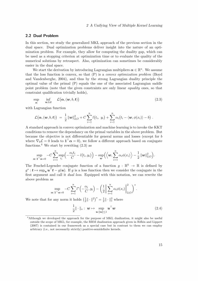
In this section, we study the generalized MKL approach of the previous section in thedual space. Dual optimization problems deliver insight into the nature of an opti-mization problem. For example, they allow for computing the duality gap, which canbe used as a stopping criterion at optimization time or to evaluate the quality of thenumerical solutions by retrospect. Also, optimization can sometimes be considerablyeasier in the dual space.
We start the derivation by introducing Lagrangian multipliers α ∈ Rn. We assumethat the loss function is convex, so that (P) is a convex optimization problem (Boydand Vandenberghe, 2004), and thus by the strong Lagrangian duality principle theoptimal value of the primal (P) equals the one of the associated Lagrangian saddlepoint problem (note that the given constraints are only linear equality ones, so thatconstraint qualification trivially holds),
supα
infw,b,t
L(α, (w, b, t)
)(2.3)
with Lagrangian function
L(α, (w, b, t)
)=
1
2‖w‖22,O + C
n∑i=1
l(ti, yi
)+
n∑i=1
αi(ti − 〈w, φ(xi)〉 − b
).
A standard approach in convex optimization and machine learning is to invoke the KKTconditions to remove the dependancy on the primal variables in the above problem. Butbecause the objective is not differentiable for general norms and losses (except for bwhere ∇bL = 0 leads to 1>α = 0), we follow a different approach based on conjugatefunctions.4 We start by rewriting (2.3) as
supα:1>α=0
−Cn∑i=1
supti
(−αiti
C− l(ti, yi
))− sup
w
(⟨w,
n∑i=1
αiφ(xi)⟩− 1
2‖w‖22,O
).
The Fenchel-Legendre conjugate function of a function g : Rk → R is defined byg∗ : t 7→ supu u
>t− g(u). If g is a loss function then we consider the conjugate in thefirst argument and call it dual loss. Equipped with this notation, we can rewrite theabove problem as
supα:1>α=0
−Cn∑i=1
l∗(−αiC, yi
)−(
1
2
∥∥∥∥ n∑i=1
αiφ(xi)
∥∥∥∥22,O
)∗.
We note that for any norm it holds(12‖ · ‖
2)∗
= 12‖ · ‖
2∗ where
1
2‖ · ‖∗ : w 7→ sup
u:‖u‖≤1u>w (2.4)
4Although we developed the approach for the purpose of MKL dualization, it might also be usefuloutside the scope of MKL; for example, the RRM dualization approach given in Rifkin and Lippert(2007) is contained in our framework as a special case but in contrast to them we can employarbitrary (i.e., not necessarily strictly) positive-semidefinite kernels.
15
I Introduction and Overview
denotes the dual norm (Boyd and Vandenberghe, 2004, , 3.26–3.27). Denoting the dualnorm of ‖·‖O by ‖·‖O∗ , we can remark that the norm dual to ‖·‖2,O is ‖·‖2,O∗ (e.g.,Aflalo et al., 2011). Thus we can further rewrite the above, resulting in the followingdual MKL optimization problem which now solely depends on α:
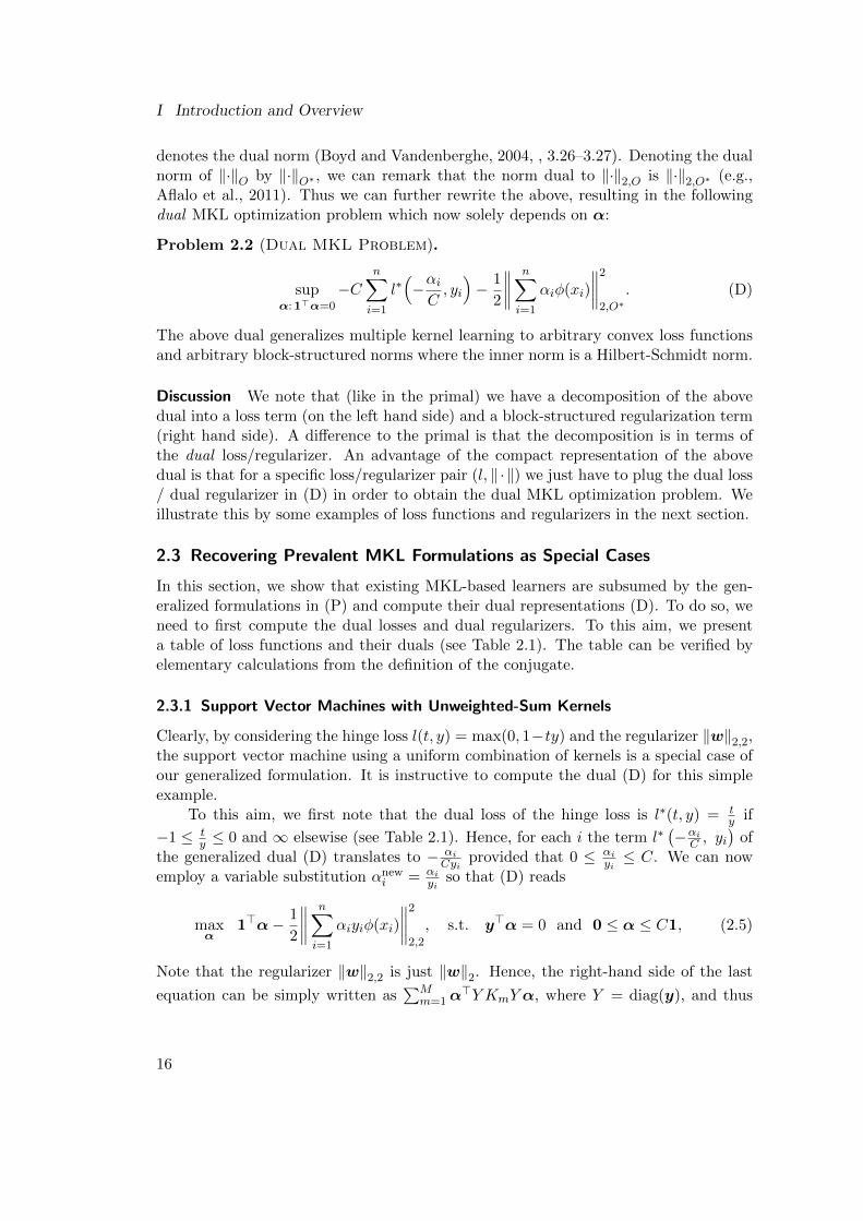
Problem 2.2 (Dual MKL Problem).
supα:1>α=0
−Cn∑i=1
l∗(−αiC, yi
)− 1
2
∥∥∥∥ n∑i=1
αiφ(xi)
∥∥∥∥22,O∗
. (D)
The above dual generalizes multiple kernel learning to arbitrary convex loss functionsand arbitrary block-structured norms where the inner norm is a Hilbert-Schmidt norm.
Discussion We note that (like in the primal) we have a decomposition of the abovedual into a loss term (on the left hand side) and a block-structured regularization term(right hand side). A difference to the primal is that the decomposition is in terms ofthe dual loss/regularizer. An advantage of the compact representation of the abovedual is that for a specific loss/regularizer pair (l, ‖ ·‖) we just have to plug the dual loss/ dual regularizer in (D) in order to obtain the dual MKL optimization problem. Weillustrate this by some examples of loss functions and regularizers in the next section.
2.3 Recovering Prevalent MKL Formulations as Special Cases
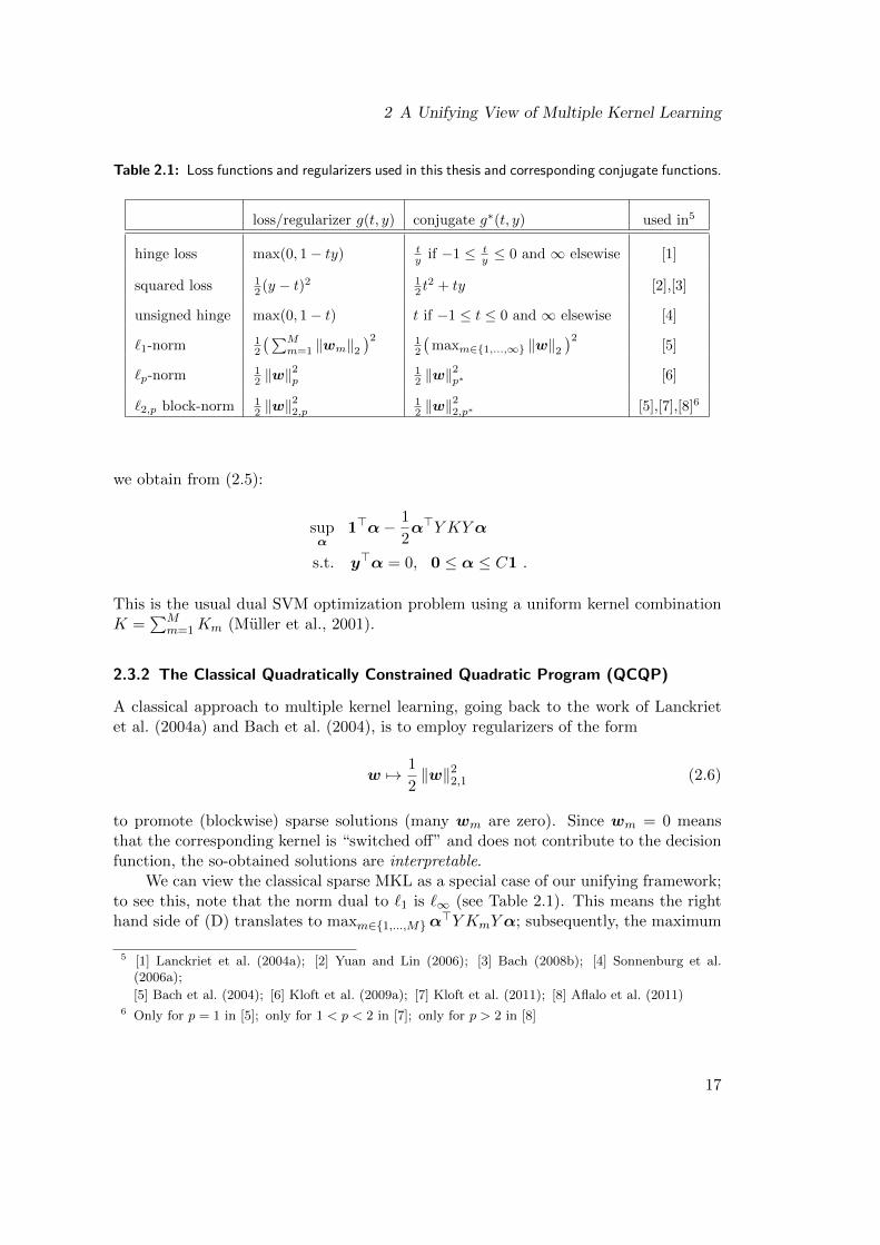
In this section, we show that existing MKL-based learners are subsumed by the gen-eralized formulations in (P) and compute their dual representations (D). To do so, weneed to first compute the dual losses and dual regularizers. To this aim, we presenta table of loss functions and their duals (see Table 2.1). The table can be verified byelementary calculations from the definition of the conjugate.
2.3.1 Support Vector Machines with Unweighted-Sum Kernels
Clearly, by considering the hinge loss l(t, y) = max(0, 1−ty) and the regularizer ‖w‖2,2,the support vector machine using a uniform combination of kernels is a special case ofour generalized formulation. It is instructive to compute the dual (D) for this simpleexample.
To this aim, we first note that the dual loss of the hinge loss is l∗(t, y) = ty if
−1 ≤ ty ≤ 0 and ∞ elsewise (see Table 2.1). Hence, for each i the term l∗
(−αiC , yi
)of
the generalized dual (D) translates to − αiCyi
provided that 0 ≤ αiyi≤ C. We can now
employ a variable substitution αnewi = αi
yiso that (D) reads
maxα
1>α− 1
2
∥∥∥∥ n∑i=1
αiyiφ(xi)
∥∥∥∥22,2
, s.t. y>α = 0 and 0 ≤ α ≤ C1, (2.5)
Note that the regularizer ‖w‖2,2 is just ‖w‖2. Hence, the right-hand side of the last
equation can be simply written as∑M
m=1α>Y KmYα, where Y = diag(y), and thus
16
2 A Unifying View of Multiple Kernel Learning
Table 2.1: Loss functions and regularizers used in this thesis and corresponding conjugate functions.
loss/regularizer g(t, y) conjugate g∗(t, y) used in5
hinge loss max(0, 1− ty) ty if −1 ≤ t
y ≤ 0 and ∞ elsewise [1]
squared loss 12 (y − t)2 1
2 t2 + ty [2],[3]
unsigned hinge max(0, 1− t) t if −1 ≤ t ≤ 0 and ∞ elsewise [4]
`1-norm 12
(∑Mm=1 ‖wm‖2
)2 12
(maxm∈1,...,∞ ‖w‖2
)2[5]
`p-norm 12 ‖w‖
2p
12 ‖w‖
2p∗ [6]
`2,p block-norm 12 ‖w‖
22,p
12 ‖w‖
22,p∗ [5],[7],[8]6
we obtain from (2.5):
supα
1>α− 1
2α>Y KYα
s.t. y>α = 0, 0 ≤ α ≤ C1 .
This is the usual dual SVM optimization problem using a uniform kernel combinationK =
∑Mm=1Km (Muller et al., 2001).
2.3.2 The Classical Quadratically Constrained Quadratic Program (QCQP)
A classical approach to multiple kernel learning, going back to the work of Lanckrietet al. (2004a) and Bach et al. (2004), is to employ regularizers of the form
w 7→ 1
2‖w‖22,1 (2.6)
to promote (blockwise) sparse solutions (many wm are zero). Since wm = 0 meansthat the corresponding kernel is “switched off” and does not contribute to the decisionfunction, the so-obtained solutions are interpretable.
We can view the classical sparse MKL as a special case of our unifying framework;to see this, note that the norm dual to `1 is `∞ (see Table 2.1). This means the righthand side of (D) translates to maxm∈1,...,Mα
>Y KmYα; subsequently, the maximum
5 [1] Lanckriet et al. (2004a); [2] Yuan and Lin (2006); [3] Bach (2008b); [4] Sonnenburg et al.(2006a);
[5] Bach et al. (2004); [6] Kloft et al. (2009a); [7] Kloft et al. (2011); [8] Aflalo et al. (2011)6 Only for p = 1 in [5]; only for 1 < p < 2 in [7]; only for p > 2 in [8]
17
I Introduction and Overview
can be expanded into a slack variable ξ, resulting in
supα,ξ
1>α− ξ
s.t. ∀m :1
2α>Y KmYα ≤ ξ ; y>α = 0 ; 0 ≤ α ≤ C1,
which is the original QCQP formulation of MKL, first given by Lanckriet et al. (2004a).
2.3.3 A Smooth Variant of Group Lasso
Yuan and Lin (2006) studied the following regularized risk minimization problem knownas the group lasso,
minw
C
2
n∑i=1
(yi −
M∑m=1
⟨wm, φm(xi)
⟩)2
+1
2
M∑m=1
‖wm‖2 (2.7)
for Hm = Rdm . The above problem has been solved by active set methods in theprimal (Roth and Fischer, 2008). We sketch an alternative approach based on dualoptimization. First, we note that the dual of l(t, y) = 1
2(y − t)2 is l∗(t, y) = 12 t
2 + tyand thus the corresponding group lasso dual according to (D) can be written as
maxα
y>α− 1
2C‖α‖22 −
1
2
∥∥∥∥(α>Y KmYα)Mm=1
∥∥∥∥∞, (2.8)
which can be expanded into the following QCQP
supα,ξ
y>α− 1
2C‖α‖22 − ξ (2.9)
s.t. ∀m :1
2α>Y KmYα ≤ ξ.
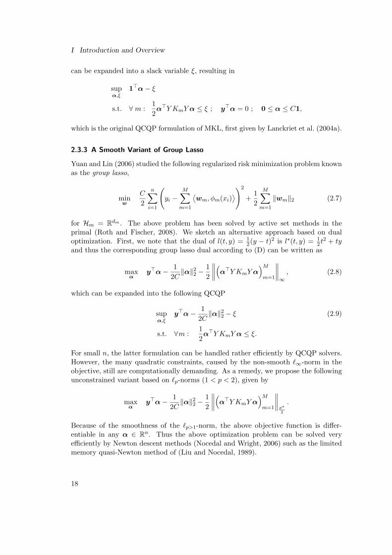
For small n, the latter formulation can be handled rather efficiently by QCQP solvers.However, the many quadratic constraints, caused by the non-smooth `∞-norm in theobjective, still are computationally demanding. As a remedy, we propose the followingunconstrained variant based on `p-norms (1 < p < 2), given by
maxα
y>α− 1
2C‖α‖22 −
1
2
∥∥∥∥(α>Y KmYα)Mm=1
∥∥∥∥p∗2
.
Because of the smoothness of the `p>1-norm, the above objective function is differ-entiable in any α ∈ Rn. Thus the above optimization problem can be solved veryefficiently by Newton descent methods (Nocedal and Wright, 2006) such as the limitedmemory quasi-Newton method of (Liu and Nocedal, 1989).
18
2 A Unifying View of Multiple Kernel Learning
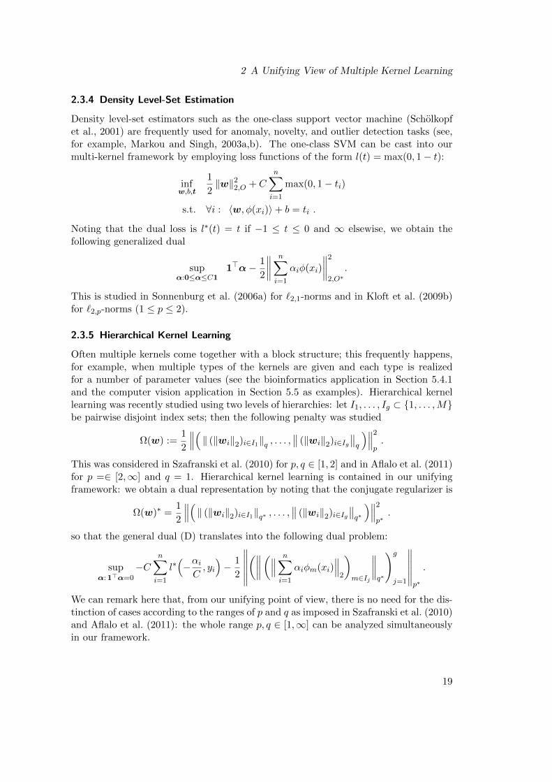
2.3.4 Density Level-Set Estimation
Density level-set estimators such as the one-class support vector machine (Scholkopfet al., 2001) are frequently used for anomaly, novelty, and outlier detection tasks (see,for example, Markou and Singh, 2003a,b). The one-class SVM can be cast into ourmulti-kernel framework by employing loss functions of the form l(t) = max(0, 1− t):
infw,b,t
1
2‖w‖22,O + C
n∑i=1
max(0, 1− ti)
s.t. ∀i : 〈w, φ(xi)〉+ b = ti .
Noting that the dual loss is l∗(t) = t if −1 ≤ t ≤ 0 and ∞ elsewise, we obtain thefollowing generalized dual
supα:0≤α≤C1
1>α− 1
2
∥∥∥∥ n∑i=1
αiφ(xi)
∥∥∥∥22,O∗
.
This is studied in Sonnenburg et al. (2006a) for `2,1-norms and in Kloft et al. (2009b)for `2,p-norms (1 ≤ p ≤ 2).
2.3.5 Hierarchical Kernel Learning
Often multiple kernels come together with a block structure; this frequently happens,for example, when multiple types of the kernels are given and each type is realizedfor a number of parameter values (see the bioinformatics application in Section 5.4.1and the computer vision application in Section 5.5 as examples). Hierarchical kernellearning was recently studied using two levels of hierarchies: let I1, . . . , Ig ⊂ 1, . . . ,Mbe pairwise disjoint index sets; then the following penalty was studied
Ω(w) :=1
2
∥∥∥( ‖ (‖wi‖2)i∈I1‖q , . . . ,∥∥ (‖wi‖2)i∈Ig
∥∥q
)∥∥∥2p.
This was considered in Szafranski et al. (2010) for p, q ∈ [1, 2] and in Aflalo et al. (2011)for p =∈ [2,∞] and q = 1. Hierarchical kernel learning is contained in our unifyingframework: we obtain a dual representation by noting that the conjugate regularizer is
Ω(w)∗ =1
2
∥∥∥( ‖ (‖wi‖2)i∈I1‖q∗ , . . . ,∥∥ (‖wi‖2)i∈Ig
∥∥q∗
)∥∥∥2p∗.
so that the general dual (D) translates into the following dual problem:
supα:1>α=0
−Cn∑i=1
l∗(−αiC, yi
)− 1
2
∥∥∥∥∥∥(∥∥∥∥(∥∥∥ n∑
i=1
αiφm(xi)∥∥∥2
)m∈Ij
∥∥∥∥q∗
)gj=1
∥∥∥∥∥∥p∗
.
We can remark here that, from our unifying point of view, there is no need for the dis-tinction of cases according to the ranges of p and q as imposed in Szafranski et al. (2010)and Aflalo et al. (2011): the whole range p, q ∈ [1,∞] can be analyzed simultaneouslyin our framework.
19
I Introduction and Overview
2.3.6 Non-Isotropic Norms
In practice, it is often desirable for an expert to incorporate prior knowledge about theproblem domain. For instance, an expert could provide estimates of the interactions ofthe kernel matrices K1, . . . ,KM in the form of an M×M matrix E. For example, if thekernels are related by an underlying graph structure, E could be the graph Laplacian(von Luxburg, 2007) encoding the similarities of the kernel matrices.
Alternatively, E could be estimated from data by computing the pairwise kernelalignments Eij =
<Ki,Kj>‖Ki‖ ‖Kj‖ (given an inner product on the space of kernel matrices
such as the Frobenius dot product).In a third scenario, E could be a diagonal matrix encoding the a priori importance
of kernels—it might be known from pilot studies that a subset of the employed kernelsis inferior to the remaining ones.
All those scenarios are subsumed by the proposed framework by considering non-isotropic regularizers of the form
Ω(w) :=1
2‖w‖2E−1
where‖w‖E−1 :=
√w>E−1w
for some E 0, where E−1 is the matrix inverse of E. The dual norm of ‖ · ‖E−1 is‖ ·‖E (this is easily verified by setting the gradient of the conjugate of 1
2‖ ·‖2E−1 to zero)
so that we obtain from (D) the dual optimization problem
supα:1>α=0
− Cn∑i=1
l∗(−αiC, yi
)− 1
2
∥∥∥∥ n∑i=1
αiφ(xi)
∥∥∥∥2E
,
which is a non-isotropic MKL problem. The usage of non-isotropic MKL was firstproposed in Varma and Ray (2007) for the very simple case of E being a diagonalmatrix and generalized in Kloft et al. (2011).
2.4 Summary and Discussion
The standard view of multiple kernel learning (introduced in the introduction) has afew limitations: first, obviously, it is incomplete since it does not account for p > 2(Kloft et al., 2010a); second, there exist convex MKL variants (again, correspondingto p > 2) that, in the standard view, cannot be represented in convex form, althoughinherently being convex (Aflalo et al., 2011); third, as it will turn out, the standardview is inconvenient for a theoretical generalization analysis such as the one carried outin Chapter 4 of this thesis.
As a remedy, we developed a rigorous mathematical framework for the problem ofmultiple kernel learning in this chapter. It comprises most existing lines of research inthat area, including very recent and seemingly different ones (e.g., the one consideredin Aflalo et al., 2011). Deviating from standard introductions, we phrased MKL as
20
2 A Unifying View of Multiple Kernel Learning
a general optimization criterion based on structured regularization, covering and alsounifying existing formulations under a common umbrella. By plugging arbitrary convexloss functions and norms into the general framework, many existing approaches can berecovered as instantiations of our model.
The unifying framework allows us to analyze a large variety of MKL methodsjointly, as exemplified by deriving a general dual representation of the criterion, withoutmaking assumptions on the employed norms and losses, besides the latter being convex.This delivers insights into connections between existing MKL formulations and, evenmore importantly, can be used to derive novel MKL formulations as special cases of ourframework, as done in the next part of the thesis, where we propose `p-norm multiplekernel learning. We note that in the most basic special case, the classical `1-normMKL formulation of Lanckriet et al. (2004a) is recovered by plugging the hinge lossand the `1-norm into the framework. Historically, the structured view of classical MKLis known since Bach et al. (2004). Here, we show that, more generally, the whole familyof MKL methods can be viewed as structured regularization (Obozinski et al., 2011), ofwhich we argue that it is a more elegant way to view MKL than the standard approach.
21

Part II
`p-norm Multiple Kernel Learning
23

II `p-norm Multiple Kernel Learning
In the previous chapter we presented a general view of MKL. However, at some pointwe have to make a particular choice of a norm, for example, in order to employ MKLin practical applications.
The main contribution of this thesis is a novel MKL formulation called `p-norm mul-tiple kernel learning. Our interest in this stems from the fact that (in contrast to theprevalent MKL variants) it has a good chance to improve on the trivial uniform-kernel-combination baseline in practical applications (we show this later in the Chapter 5 ofthis thesis).
We obtain `p-norm MKL from the unifying MKL framework by using the regularizer
Ωmkl(w) =1
2‖w‖22,p, p ∈ 1, . . . ,∞,
where the `2,p-norm is defined as
‖w‖2,p :=
( M∑m=1
‖wm‖p2) 1p
for p ∈ [1,∞[ and ‖w‖2,p := supm=1,...,M ‖wm‖2 for p = ∞. Plugging this into theunifying optimization problems (Problems 2.1 and 2.2) we obtain the `p-norm MKLprimal and dual problems:
Problem II.3 (`p-norm MKL). For any p ∈ [1,∞],
infw,b,t
1
2‖w‖22,p + C
n∑i=1
l(ti, yi
)(Primal)
s.t. ∀i : 〈w, φ(xi)〉+ b = ti ,
supα:1>α=0
− Cn∑i=1
l∗(−αiC, yi
)− 1
2
∥∥∥∥ n∑i=1
αiφ(xi)
∥∥∥∥22,p∗
. (Dual)
The key difference of `p>1-norm MKL to previous MKL approaches, which are basedon `1-norms, is that the obtained weight vectors are unlikely to be sparse. This wasalready indicated in the introduction and is now discussed in more detail here: theoptimal solution of the `p-norm MKL optimization problem is attained when the norm
25
II `p-norm Multiple Kernel Learning
||x||1=1
quatric
||x||2=1
quatric
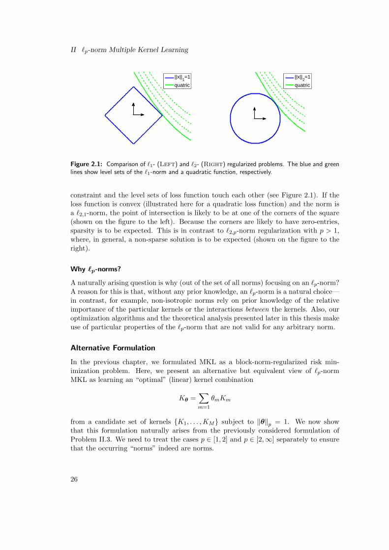
Figure 2.1: Comparison of `1- (Left) and `2- (Right) regularized problems. The blue and greenlines show level sets of the `1-norm and a quadratic function, respectively.
constraint and the level sets of loss function touch each other (see Figure 2.1). If theloss function is convex (illustrated here for a quadratic loss function) and the norm isa `2,1-norm, the point of intersection is likely to be at one of the corners of the square(shown on the figure to the left). Because the corners are likely to have zero-entries,sparsity is to be expected. This is in contrast to `2,p-norm regularization with p > 1,where, in general, a non-sparse solution is to be expected (shown on the figure to theright).
Why `p-norms?
A naturally arising question is why (out of the set of all norms) focusing on an `p-norm?A reason for this is that, without any prior knowledge, an `p-norm is a natural choice—in contrast, for example, non-isotropic norms rely on prior knowledge of the relativeimportance of the particular kernels or the interactions between the kernels. Also, ouroptimization algorithms and the theoretical analysis presented later in this thesis makeuse of particular properties of the `p-norm that are not valid for any arbitrary norm.
Alternative Formulation
In the previous chapter, we formulated MKL as a block-norm-regularized risk min-imization problem. Here, we present an alternative but equivalent view of `p-normMKL as learning an “optimal” (linear) kernel combination
Kθ =∑m=1
θmKm
from a candidate set of kernels K1, . . . ,KM subject to ‖θ‖p = 1. We now showthat this formulation naturally arises from the previously considered formulation ofProblem II.3. We need to treat the cases p ∈ [1, 2] and p ∈ [2,∞] separately to ensurethat the occurring “norms” indeed are norms.
26
The case p ∈ [1, 2[
We first deal with the case p ∈ [1, 2[, which corresponds to the established standardview of MKL. To this aim, we reconsider the regularizer of Problem II.3 and note thatfor p ∈ [1, 2] we can rewrite it as
∥∥ n∑i=1
αiφ(xi)∥∥22,p∗
=∥∥∥(α>Kmα
)Mm=1
∥∥∥p∗/2
(2.4)= sup
θ: ‖θ‖(p∗/2)∗≤1
M∑m=1
θmα>Kmα (II.1)
where we use the definition of the dual norm (Equation (2.4)). Note that the choiceof p ∈ [1, 2] ensures that the above “norm” really is a norm: indeed, p ∈ [1, 2] impliesthat p∗/2 is in the valid interval [1,∞]. We also note that (p∗/2)∗ = p
2−p and that theoptimal θ is nonnegative so that we can use (II.1) to rewrite Problem II.3 as
infθ: ‖θ‖p/(2−p)≤1
svm(Kθ), s.t. Kθ =
M∑m=1
θmKm , (II.2)
where we use the shorthand
svm(Kθ) := supα:1>α=0
−Cn∑i=1
l∗(−αiC, yi
)− 1
2α>Kθα (II.3)
to denote the optimal value of the SVM optimization problem. Note that we exchangedthe sequence of minimization and maximization to obtain (II.2), which is justified bySion’s Minimax theorem (Sion, 1958). Equation (II.2) gives an alternative formulationof the `p-norm MKL problem: training a support vector machine which simultaneouslyalso optimizes over the optimal kernel combination (subject to a norm constraint onthe combination coefficients to avoid overfitting).
The case p ∈ ]2,∞]
Unfortunately, we cannot use the above approach in the case p ∈ [2,∞] as then thenorm parameter p/(2− p) lies outside the valid range of [1,∞]. However, we can usea similar argument as above by considering the primal of Problem II.3 instead of thedual: the primal regularizer of Problem II.3 can be rewritten as
‖w‖22,p =∥∥∥( ‖wm‖22
)Mm=1
∥∥∥p/2
(2.4)= sup
θ: ‖θ‖(p/2)∗≤1
M∑m=1
θm ‖wm‖22
= supθ:
∑m θ−(p/2)∗m ≤1
M∑m=1
θ−1m ‖wm‖22 . (II.4)
27
II `p-norm Multiple Kernel Learning
since p/2 is in the valid interval [1,∞] for p ∈ [2,∞]. We note that −(p/2)∗ = p/(2−p)and that the optimal θ is nonnegative; hence, the primal of Problem II.3 translatesinto
supθ:
∑m θ
p/(2−p)m ≤1
svm(Kθ), s.t. Kθ =
M∑m=1
θmKm ,
with svm(Kθ) := infw,b
1
2
M∑m=1
θ−1m ‖wm‖22 + Cn∑i=1
l(〈w, φ(xi)〉+ b, yi
).
Remark
Note that in the above definition of the svm function there is no collision with thedefinition in (II.3) since both formulations are dual to each other, for any fixed θ ≥ 0.One way to see this is by introducing slack variables ti := 〈w, φ(xi)〉+ b to write theabove as
svm(Kθ) = infw,b,t
1
2
M∑m=1
θ−1m ‖wm‖22 + Cn∑i=1
l(ti, yi
)and then incorporating the constraints by Lagrangian multipliers αi:
supα
infw,b,t
1
2
M∑m=1
θ−1m ‖wm‖22 + C
n∑i=1
l(ti, yi
)+
n∑i=1
αi(ti − 〈w, φ(xi)〉 − b
).
The KKT conditions, which can be used to compute the decision function and to recoverthe treshold b, hold for the pair (w,α) and yield
∀m = 1, . . . ,M : ‖wm‖22 = θ2mαKmα . (II.5)
Note, furthermore, that applying the KKT conditions to (2.3) for `p-norms yields:
∃ c > 0 : ‖wm‖ = c (αKmα)1
2(p−1) , (II.6)
The remainder of the dualization is analogue to what we have seen above and yields(II.3).
Putting the Pieces Together...
Putting things together, we obtain the following alternative MKL optimization problem.
Problem II.4 (`p-norm MKL, Alternative Formulation). The alternative for-mulation of `p-norm multiple kernel learning is given by
infθ≥0
svm(Kθ), ( if p ∈ [1, 2[ )
supθ≥0
svm(Kθ), ( if p ∈]2,∞] )
s.t. Kθ =
M∑m=1
θmKm,∑m
θp/(2−p)m ≤ 1,
28
where svm denotes the optimal objective value of the SVM optimization problem,
svm(Kθ) := infw,b
1
2
M∑m=1
θ−1m ‖wm‖22 + C
n∑i=1
l(〈w, φ(xi)〉+ b, yi
)= supα:1>α=0
− Cn∑i=1
l∗(−αiC, yi
)− 1
2α>Kθα .
The above problem can be interpreted as finding or “learning” an optimal kernel com-bination from a set of kernels where the quality of the mixtures is evaluated in termsof the SVM objective function. This alternative view is much in the original learning-kernels spirit of Lanckriet et al. (2004a): “Learning the kernel matrix with semi-definiteprogramming”.
Remaining Contents of this Part
In the remainder of this part we derive optimization algorithms for `p-norm MKL andapply them in order to empirically analyze the generalization performance of `p-normMKL in controlled artificial environments as well as real-world applications from thedomains of bioinformatics and computer vision. We also investigate `p-norm MKLtheoretically and show that for a large range of learning scenarios it enjoys strongergeneralization guarantees than classical MKL and the SVM using a uniform kernelcombination.
29

3 Algorithms
3 Algorithms
In this chapter, we present two optimization algorithms for the `p-norm MKL prob-lem II.3. Each algorithm has its own advantage: while the first one is provably conver-gent, easier to implement, and also to modify, due to its modular design, the secondone is expected to be faster in practice and also less memory-intensive. For the sakeof performance, both algorithms were implemented in C++ and made available as apart of the open source machine learning toolbox SHOGUN (Sonnenburg et al., 2010),which also contains interfaces to MATLAB, Octave, Phyton, and R.
Both algorithms are based on the alternative `p-norm MKL formulation (Prob-lem II.4) in contrast to the original problem (Problem II.3). This is because the formerconsists of an “inner” and an “outer” optimization problem, where the inner problemis a standard SVM optimization problem. This has the advantage that existing (highlyoptimized) SVM solvers can be exploited.
We remark that the proposed algorithms can, in particular, be used to optimizethe classical `p=1-norm MKL formulation. In the computational experiments at theend of this chapter, we show that the proposed algorithms outperform the prevalentstate-of-the-art solvers by up to two magnitudes.
The main contributions in this chapter are the following:
• We present a novel optimization method based on a simple, analytical formula, which,in particular, can be used to optimize classical MKL.
• We prove its convergence for p > 1.
• We implement the algorithm as an interleaved chunking optimizer in C++ within theSHOGUN toolbox with interfaces to MATLAB, Octave, Phyton, and R.
• We show that our implementation allows for training with up to ten thousands of datapoints and thousands of kernels, while the state-of-the-art approaches run already outof memory with a few thousand of data points and hundreds of kernels.
• Even for moderate sizes of the training and kernel sets, our approach outperformsprevalent ones by up to two magnitudes.
Parts of this chapter are based on:
M. Kloft, U. Brefeld, S. Sonnenburg, P. Laskov, K.-R. Muller, and A. Zien. Efficientand accurate lp-norm multiple kernel learning. In Advances in Neural InformationProcessing Systems 22 (NIPS 2009), pages 997–1005. MIT Press, 2009.
M. Kloft, U. Brefeld, S. Sonnenburg, and A. Zien. Lp-norm multiple kernel learning.Journal of Machine Learning Research (JMLR), 12:953–997, 2011.
3.1 Block Coordinate Descent Algorithm
The main idea of the first approach is to divide the set of optimization variables (whichis θ1, . . . , θM , α1, . . . , αn) into two groups—the set θ1, . . . , θM on one hand and theset α1, ..., αM on the other—and then alternating the optimization with respect to θwith the one with respect to α.
31
II `p-norm Multiple Kernel Learning
We observe that in the α-step this boils down to training a standard SVM. Incontrast, the θ-step can simply be performed by means of an analytical formula, as thefollowing proposition shows.
Proposition 3.1. Given any (possibly suboptimal) w 6= 0 in the objective of Prob-lem II.4, the optimal θ is attained for
∀m = 1, . . . ,M : θm =‖wm‖2−p2(∑M
m′=1 ‖wm′‖p2)(2−p)/p . ( if p ∈ [1, 2[ )
Assume at least one of the kernel matrices Km is strictly positive-definite. Then, givenany (possibly suboptimal) α 6= 0, the optimal θ is attained for
∀m = 1, . . . ,M : θm =
(α>Kmα
)− 2−p2−2p(∑M
m′=1
(α>Km′α
)− p2−2p
)(2−p)/p . ( if p ∈]2,∞] )
Proof To start the proof, we consider Problem II.4, fix the variables w, b, and onlyoptimize w.r.t θ. By Lemma B.1 we can write this as Tikhonov regularized problem:
infθ≥0
1
2
M∑m=1
θ−1m ‖wm‖22 + C
n∑i=1
l(〈w, φ(xi)〉+ b, yi
)+ µ
M∑m=1
θp/(2−p)m .
for a suitable chosen constant µ > 0. Let us ignore the positivity constraint θ ≥ 0 forthe moment; the above objective is differentiable in θ for θ 6= 0 so that the optimumis attained for the gradient w.r.t. θ being zero, i.e.,
∀m = 1, . . . ,M : −1
2θ−2m ‖wm‖2 + µ p/(2− p) θ(p/(2−p))−1m = 0 .
Solving this for θ, we observe that the optimal θ is indeed positive and we have theproportionality
∀m = 1, . . . ,M : θm ∝ ‖wm‖2−p2 .
Normalizing θ to fulfill the constraint∑
m θp/(2−p)m = 1 (which is possible because
w 6= 0) yields the first part of the proposition. Note that θm 6= 0 is no restriction asθm = 0 can only be when ‖wm‖2 = 0 so that the proposition trivially holds in thatcase.
For the second part, we proceed similarly but use the dual formulation as a startingpoint: we write
infθ≥0
C
n∑i=1
l∗(−αiC, yi
)+
1
2α>
M∑m=1
θmKmα+ µ
M∑m=1
θp/(2−p)m
32
3 Algorithms
so that setting the gradient w.r.t. θ to zero yields
∀m = 1, . . . ,M : −1
2α>Kmα+ µ p/(2− p) θ(p/(2−p))−1m = 0 .
Solving this for θ results in the proportionality
∀m = 1, . . . ,M : θm ∝(α>Kmα
)− 2−p2−2p .
Again, we observe that the so-obtained θ is nonnegative and normalizing θ to fulfill
the constraint∑
m θp/(2−p)m = 1 (which is possible because ∃m : Km 0) yields the
second part of the proposition.
We now have all ingredients to formulate a simple macro-wrapper algorithm for `p-normMKL training:
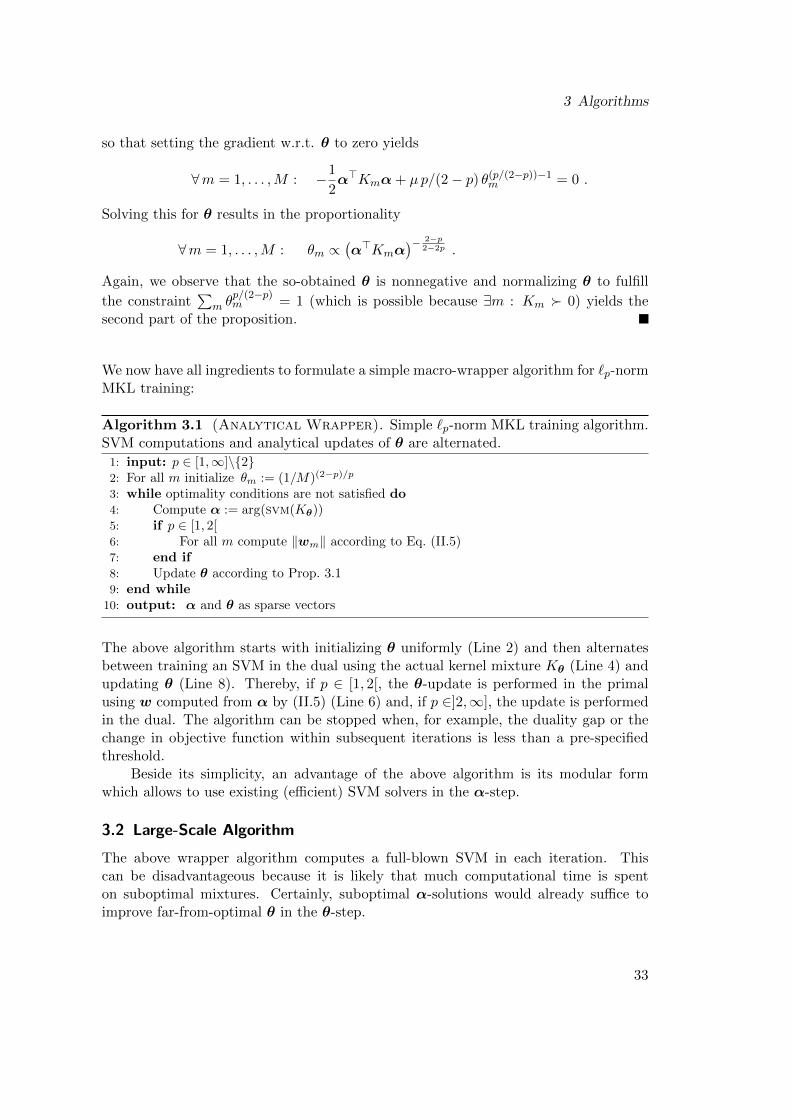
Algorithm 3.1 (Analytical Wrapper). Simple `p-norm MKL training algorithm.SVM computations and analytical updates of θ are alternated.
1: input: p ∈ [1,∞]\22: For all m initialize θm := (1/M)(2−p)/p
3: while optimality conditions are not satisfied do4: Compute α := arg(svm(Kθ))5: if p ∈ [1, 2[6: For all m compute ‖wm‖ according to Eq. (II.5)7: end if8: Update θ according to Prop. 3.19: end while
10: output: α and θ as sparse vectors
The above algorithm starts with initializing θ uniformly (Line 2) and then alternatesbetween training an SVM in the dual using the actual kernel mixture Kθ (Line 4) andupdating θ (Line 8). Thereby, if p ∈ [1, 2[, the θ-update is performed in the primalusing w computed from α by (II.5) (Line 6) and, if p ∈]2,∞], the update is performedin the dual. The algorithm can be stopped when, for example, the duality gap or thechange in objective function within subsequent iterations is less than a pre-specifiedthreshold.
Beside its simplicity, an advantage of the above algorithm is its modular formwhich allows to use existing (efficient) SVM solvers in the α-step.
3.2 Large-Scale Algorithm
The above wrapper algorithm computes a full-blown SVM in each iteration. Thiscan be disadvantageous because it is likely that much computational time is spenton suboptimal mixtures. Certainly, suboptimal α-solutions would already suffice toimprove far-from-optimal θ in the θ-step.
33
II `p-norm Multiple Kernel Learning
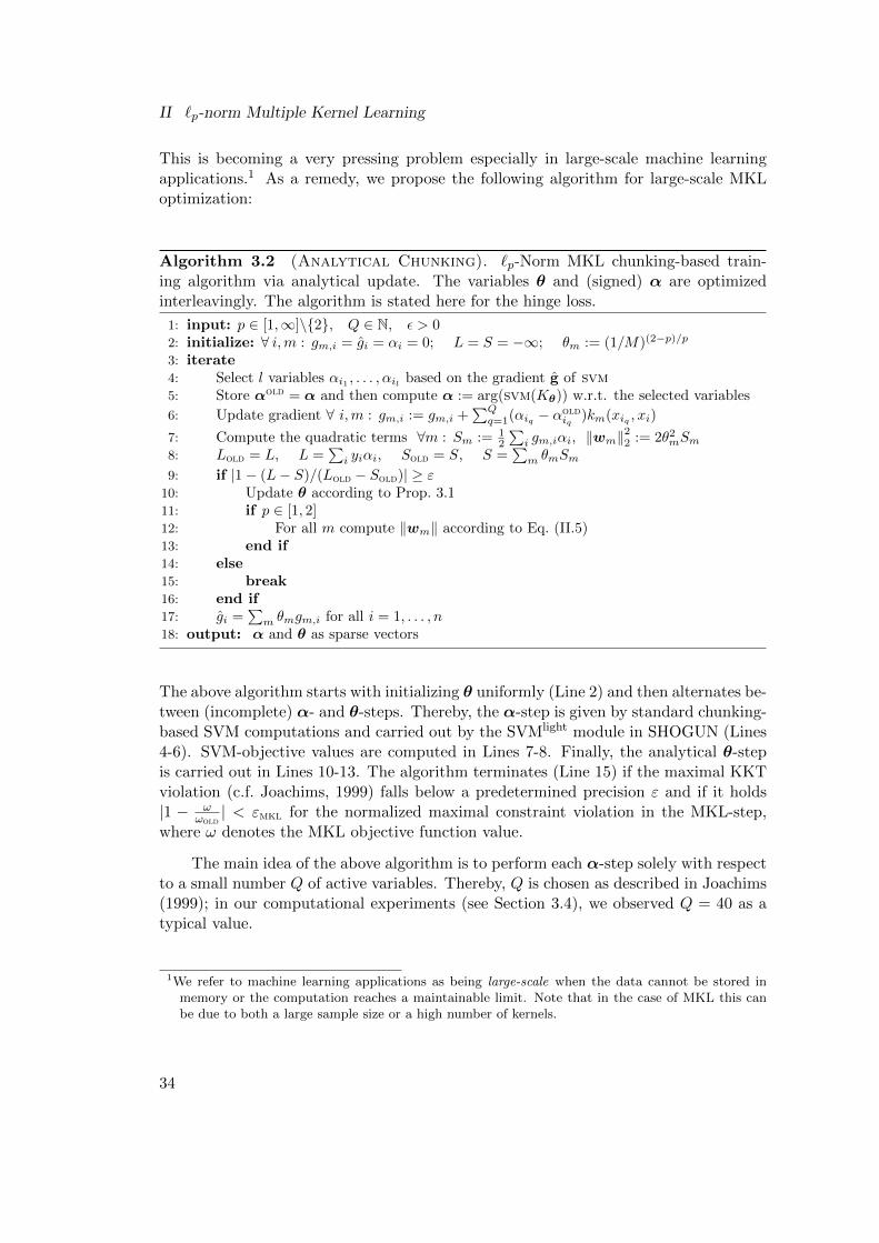
This is becoming a very pressing problem especially in large-scale machine learningapplications.1 As a remedy, we propose the following algorithm for large-scale MKLoptimization:
Algorithm 3.2 (Analytical Chunking). `p-Norm MKL chunking-based train-ing algorithm via analytical update. The variables θ and (signed) α are optimizedinterleavingly. The algorithm is stated here for the hinge loss.
1: input: p ∈ [1,∞]\2, Q ∈ N, ε > 02: initialize: ∀ i,m : gm,i = gi = αi = 0; L = S = −∞; θm := (1/M)(2−p)/p
3: iterate4: Select l variables αi1 , . . . , αil based on the gradient g of svm5: Store αold = α and then compute α := arg(svm(Kθ)) w.r.t. the selected variables
6: Update gradient ∀ i,m : gm,i := gm,i +∑Qq=1(αiq − αold
iq)km(xiq , xi)
7: Compute the quadratic terms ∀m : Sm := 12
∑i gm,iαi, ‖wm‖22 := 2θ2mSm
8: Lold = L, L =∑i yiαi, Sold = S, S =
∑m θmSm
9: if |1− (L− S)/(Lold − Sold)| ≥ ε10: Update θ according to Prop. 3.111: if p ∈ [1, 2]12: For all m compute ‖wm‖ according to Eq. (II.5)13: end if14: else15: break16: end if17: gi =
∑m θmgm,i for all i = 1, . . . , n
18: output: α and θ as sparse vectors
The above algorithm starts with initializing θ uniformly (Line 2) and then alternates be-tween (incomplete) α- and θ-steps. Thereby, the α-step is given by standard chunking-based SVM computations and carried out by the SVMlight module in SHOGUN (Lines4-6). SVM-objective values are computed in Lines 7-8. Finally, the analytical θ-stepis carried out in Lines 10-13. The algorithm terminates (Line 15) if the maximal KKTviolation (c.f. Joachims, 1999) falls below a predetermined precision ε and if it holds|1 − ω
ωold| < εmkl for the normalized maximal constraint violation in the MKL-step,
where ω denotes the MKL objective function value.
The main idea of the above algorithm is to perform each α-step solely with respectto a small number Q of active variables. Thereby, Q is chosen as described in Joachims(1999); in our computational experiments (see Section 3.4), we observed Q = 40 as atypical value.
1We refer to machine learning applications as being large-scale when the data cannot be stored inmemory or the computation reaches a maintainable limit. Note that in the case of MKL this canbe due to both a large sample size or a high number of kernels.
34
3 Algorithms
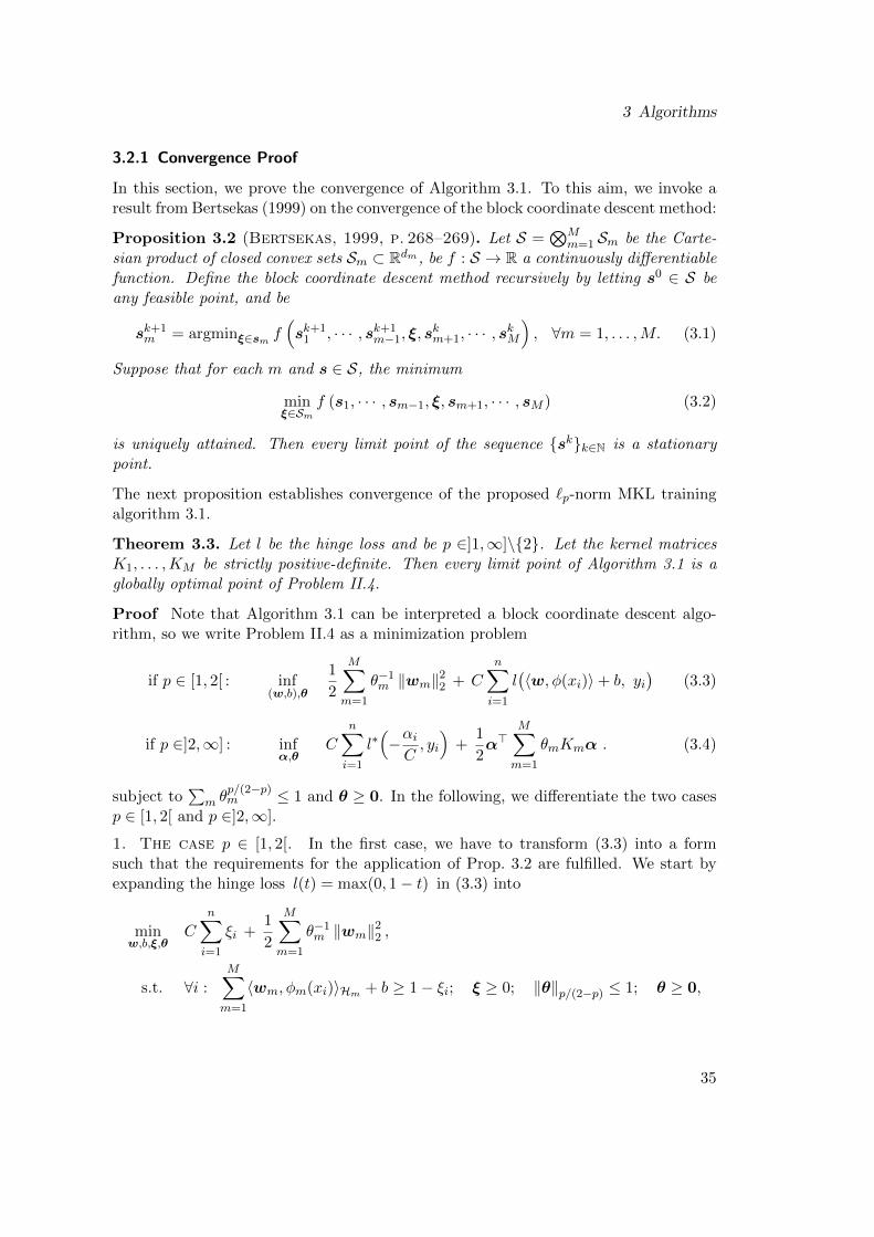
3.2.1 Convergence Proof
In this section, we prove the convergence of Algorithm 3.1. To this aim, we invoke aresult from Bertsekas (1999) on the convergence of the block coordinate descent method:
Proposition 3.2 (Bertsekas, 1999, p. 268–269). Let S =⊗M
m=1 Sm be the Carte-sian product of closed convex sets Sm ⊂ Rdm, be f : S → R a continuously differentiablefunction. Define the block coordinate descent method recursively by letting s0 ∈ S beany feasible point, and be
sk+1m = argminξ∈sm f
(sk+11 , · · · , sk+1
m−1, ξ, skm+1, · · · , skM
), ∀m = 1, . . . ,M. (3.1)
Suppose that for each m and s ∈ S, the minimum
minξ∈Sm
f (s1, · · · , sm−1, ξ, sm+1, · · · , sM ) (3.2)
is uniquely attained. Then every limit point of the sequence skk∈N is a stationarypoint.
The next proposition establishes convergence of the proposed `p-norm MKL trainingalgorithm 3.1.
Theorem 3.3. Let l be the hinge loss and be p ∈]1,∞]\2. Let the kernel matricesK1, . . . ,KM be strictly positive-definite. Then every limit point of Algorithm 3.1 is aglobally optimal point of Problem II.4.
Proof Note that Algorithm 3.1 can be interpreted a block coordinate descent algo-rithm, so we write Problem II.4 as a minimization problem
if p ∈ [1, 2[ : inf(w,b),θ
1
2
M∑m=1
θ−1m ‖wm‖22 + Cn∑i=1
l(〈w, φ(xi)〉+ b, yi
)(3.3)
if p ∈]2,∞] : infα,θ
Cn∑i=1
l∗(−αiC, yi
)+
1
2α>
M∑m=1
θmKmα . (3.4)
subject to∑
m θp/(2−p)m ≤ 1 and θ ≥ 0. In the following, we differentiate the two cases
p ∈ [1, 2[ and p ∈]2,∞].
1. The case p ∈ [1, 2[. In the first case, we have to transform (3.3) into a formsuch that the requirements for the application of Prop. 3.2 are fulfilled. We start byexpanding the hinge loss l(t) = max(0, 1− t) in (3.3) into
minw,b,ξ,θ
C
n∑i=1
ξi +1
2
M∑m=1
θ−1m ‖wm‖22 ,
s.t. ∀i :
M∑m=1
〈wm, φm(xi)〉Hm + b ≥ 1− ξi; ξ ≥ 0; ‖θ‖p/(2−p) ≤ 1; θ ≥ 0,
35
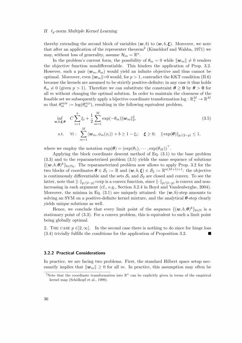
II `p-norm Multiple Kernel Learning
thereby extending the second block of variables (w, b) to (w, b, ξ). Moreover, we notethat after an application of the representer theorem2 (Kimeldorf and Wahba, 1971) wemay, without loss of generality, assume Hm = Rn.
In the problem’s current form, the possibility of θm = 0 while ‖wm‖ 6= 0 rendersthe objective function nondifferentiable. This hinders the application of Prop. 3.2.However, such a pair (wm, θm) would yield an infinite objective and thus cannot beoptimal. Moreover, even ‖wm‖=0 would, for p > 1, contradict the KKT condition (II.6)because the kernels are assumed to be strictly positive-definite; in any case it thus holdsθm 6= 0 (given p > 1). Therefore we can substitute the constraint θ ≥ 0 by θ > 0 forall m without changing the optimal solution. In order to maintain the closeness of thefeasible set we subsequently apply a bijective coordinate transformation log : RM+ → RMso that θnewm := log(θoldm ), resulting in the following equivalent problem,
infw,b,ξ,θ
Cn∑i=1
ξi +1
2
M∑m=1
exp(−θm)‖wm‖22, (3.5)
s.t. ∀i :M∑m=1
〈wm, φm(xi)〉+ b ≥ 1− ξi; ξ ≥ 0; ‖ exp(θ)‖p/(2−p) ≤ 1,
where we employ the notation exp(θ) = (exp(θ1), · · · , exp(θM ))>.Applying the block coordinate descent method of Eq. (3.1) to the base problem
(3.3) and to the reparameterized problem (3.5) yields the same sequence of solutions(w, b,θ)kk∈N0 . The reparameterized problem now allows to apply Prop. 3.2 for thetwo blocks of coordinates θ ∈ S1 := R and (w, b, ξ) ∈ S2 := Rn(M+1)+1: the objectiveis continuously differentiable and the sets S1 and S2 are closed and convex. To see thelatter, note that ‖·‖p/(2−p)exp is a convex function, since ‖·‖p/(2−p) is convex and non-increasing in each argument (cf., e.g., Section 3.2.4 in Boyd and Vandenberghe, 2004).Moreover, the minima in Eq. (3.1) are uniquely attained: the (w, b)-step amounts tosolving an SVM on a positive-definite kernel mixture, and the analytical θ-step clearlyyields unique solutions as well.
Hence, we conclude that every limit point of the sequence (w, b,θ)kk∈N is astationary point of (3.3). For a convex problem, this is equivalent to such a limit pointbeing globally optimal.
2. The case p ∈]2,∞]. In the second case there is nothing to do since for hinge loss(3.4) trivially fulfills the conditions for the application of Proposition 3.2.
3.2.2 Practical Considerations
In practice, we are facing two problems. First, the standard Hilbert space setup nec-essarily implies that ‖wm‖ ≥ 0 for all m. In practice, this assumption may often be
2Note that the coordinate transformation into Rn can be explicitly given in terms of the empiricalkernel map (Scholkopf et al., 1999).
36
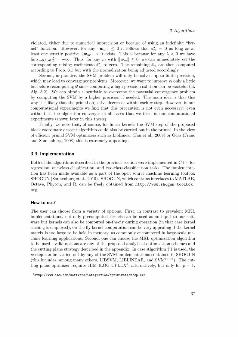
3 Algorithms
violated, either due to numerical imprecision or because of using an indefinite “ker-nel” function. However, for any ‖wm‖ ≤ 0 it follows that θ?m = 0 as long as atleast one strictly positive ‖wm′‖ > 0 exists. This is because for any λ < 0 we havelimh→0,h>0
λh = −∞. Thus, for any m with ‖wm‖ ≤ 0, we can immediately set the
corresponding mixing coefficients θ?m to zero. The remaining θm are then computedaccording to Prop. 3.1 but with the normalization being adjusted accordingly.
Second, in practice, the SVM problem will only be solved up to finite precision,which may lead to convergence problems. Moreover, we want to improve α only a littlebit before recomputing θ since computing a high precision solution can be wasteful (cf.Alg. 3.2). We can obtain a heuristic to overcome the potential convergence problemby computing the SVM by a higher precision if needed. The main idea is that thisway it is likely that the primal objective decreases within each α-step. However, in ourcomputational experiments we find that this precaution is not even necessary: evenwithout it, the algorithm converges in all cases that we tried in our computationalexperiments (shown later in this thesis).
Finally, we note that, of course, for linear kernels the SVM-step of the proposedblock coordinate descent algorithm could also be carried out in the primal. In the viewof efficient primal SVM optimizers such as LibLinear (Fan et al., 2008) or Ocas (Francand Sonnenburg, 2008) this is extremely appealing.
3.3 Implementation
Both of the algorithms described in the previous section were implemented in C++ forregression, one-class classification, and two-class classification tasks. The implementa-tion has been made available as a part of the open source machine learning toolboxSHOGUN (Sonnenburg et al., 2010). SHOGUN, which contains interfaces to MATLAB,Octave, Phyton, and R, can be freely obtained from http://www.shogun-toolbox.
org.
How to use?
The user can choose from a variety of options. First, in contrast to prevalent MKLimplementations, not only precomputed kernels can be used as an input to our soft-ware but kernels can also be computed on-the-fly during operation (in that case kernelcaching is employed); on-the-fly kernel computation can be very appealing if the kernelmatrix is too large to be held in memory, as commonly encountered in large-scale ma-chine learning applications. Second, one can choose the MKL optimization algorithmto be used—valid options are any of the proposed analytical optimization schemes andthe cutting plane strategy described in the appendix. In case Algorithm 3.1 is used, theα-step can be carried out by any of the SVM implementations contained in SHOGUN(this includes, among many others, LIBSVM, LIBLINEAR, and SVMlight). The cut-ting plane optimizer requires IBM ILOG CPLEX3; alternatively, but only for p = 1,
3http://www.ibm.com/software/integration/optimization/cplex/.
37
II `p-norm Multiple Kernel Learning
the free LP solver GLPK4 can be chosen.
Implementation Details
Both, the cutting plane strategy and the analytical algorithm (Algorithm 3.2) performinterleaved optimization and thus require modification of the core SVM optimization al-gorithm. This is currently integrated into the chunking-based SVRlight and SVMlight.To reduce the implementation effort, we implement a single function perform mkl -
step(lin, quad), that has two arguments: first, the linear term lin :=∑n
i=1 αi and
second, an array quad =(quadm
)Mm=1
containing the quadratic terms of the respective
kernels quadm := 12α
TKmα. This function is either, in the interleaved optimizationcase, called as a callback function (after each chunking step), or it is called by thewrapper algorithm (after each SVM optimization to full precision).
One-class classification is trivially implemented using lin = 0 and support vectorregression (SVR) is typically performed by internally translating the SVR probleminto a standard SVM classification problem with twice the number of examples (oncepositively and once negatively labeled with corresponding α and α∗). Thus one needsdirect access to α∗ and computes lin = −
∑ni=1(αi+α
∗i )ε−
∑ni=1(αi−α∗i )yi. Since this
requires modification of the core SVM solver, we implement SVR only for interleavedoptimization and SVMlight.
Note that the choice of the size of the kernel cache becomes crucial when applyingMKL to large-scale learning applications. While conventional wrapper algorithms onlysolve a single kernel SVM in each iteration and thus use a single large kernel cache,interleaved optimization methods must keep track of several partial MKL objectivesobjm and thus require access to individual kernel rows. Therefore, the same cache sizeshould be used for all sub-kernels.
3.3.1 Kernel Normalization
In practice, the normalization of kernels is as important for MKL as the normalizationof features is for training regularized linear or single-kernel models. This is owed to thebias introduced by the regularization: optimal feature / kernel weights are requestedto be small. This is easier to achieve for features (or entire feature spaces, as impliedby kernels) that are scaled to be of large magnitude, while downscaling them wouldrequire a correspondingly upscaled weight for representing the same predictive model.Upscaling (downscaling) features is thus equivalent to modifying regularizers so thatthey penalize those features less (more). We here use isotropic regularizers, whichpenalize all dimensions uniformly. This implies that the kernels have to be normalizedin a sensible way in order to represent an “uninformative prior” as to which kernels areuseful.
There exist several approaches to kernel normalization, of which we use two in thecomputational experiments below. They are fundamentally different. The first one gen-eralizes the common practice of standardizing features to entire kernels, thereby directly
4http://www.gnu.org/software/glpk/.
38
3 Algorithms
implementing the spirit of the discussion above. In contrast, the second normalizationapproach rescales the data points to unit norm in feature space. Nevertheless, it canhave a beneficial effect on the scaling of kernels, as we argue below.
Both normalization approaches, as well as a number of additional ones, were imple-mented and made available as a part of our SHOGUN implementation (see SHOGUNdocumentation for a complete list of normalization methods).
Method 1: Multiplicative Normalization
As proposed in Ong and Zien (2008), we can multiplicatively normalize the kernels tohave uniform variance of data points in feature space. Formally, we find a positiverescaling ρm of the kernel so that the rescaled kernel km(·, ·) = ρmkm(·, ·) and thecorresponding feature map Φm(·) =
√ρmΦm(·) satisfy
1
n
n∑i=1
∥∥∥Φm(xi)− Φm(x)∥∥∥2 = 1
for each m = 1, . . . ,M , where Φm(x) := 1n
∑ni=1 Φm(xi) is the empirical mean of the
data in feature space. It is straightforward to verify that the above equation can beequivalently be expressed in terms of kernel functions as
1
n
n∑i=1
km(xi, xi)−1
n2
n∑i=1
n∑j=1
km(xi, xj) = 1,
so that the final normalization rule is
k(x, x) 7−→ k(x, x)1n
∑ni=1 k(xi, xi)− 1
n2
∑ni,j=1, k(xi, xj)
. (3.6)
Note that in case the kernel is centered (i.e. the empirical mean of the data points lieson the origin), the above rule simplifies to k(x, x) 7−→ k(x, x)/ 1
ntr(K), where tr(K) :=∑ni=1 k(xi, xi) is the trace of the kernel matrix K.
Method 2: Spherical Normalization
Another approach, which is frequently applied in the MKL literature, is to normalize
k(x, x) 7−→ k(x, x)√k(x, x)k(x, x)
. (3.7)
After this operation, ‖x‖ = k(x, x) = 1 holds for each data point x; this means that eachdata point is rescaled to lie on the unit sphere. Still, this also may have an effect on thescale of the features: a centered, spherically normalized kernel is also multiplicativelynormalized because, for centered kernels, the multiplicative normalization rule becomesk(x, x) 7−→ k(x, x)/ 1
ntr(K) = k(x, x)/1.
39
II `p-norm Multiple Kernel Learning
Thus, spherical normalization may be seen as an approximation of multiplicativenormalization and may be used as a substitute for it. Note, however, that it changesthe data points themselves by eliminating length information; whether this is desiredor not depends on the learning task at hand (for example, in text classification, thecategory of a text rather depends on its word frequency distribution than on its lengthso that spherical normalization is desired).
3.4 Runtime Experiments
In this section, we analyze the efficiency of our implementation of `p-norm MKL. Weexperiment on the MNIST data set, where the task is to separate odd and even dig-its. The digits in this n = 60, 000-elemental data set, which we downloaded fromhttp://yann.lecun.com/exdb/mnist/, are of size 28x28, leading to d = 784 dimen-sional examples. We compare the proposed optimization approaches for `p-norm MKLwith the state-of-the-art for `1-norm MKL, namely, SimpleMKL (Rakotomamonjyet al., 2008), HessianMKL (Chapelle and Rakotomamonjy, 2008), and the cutting planemethod (CPM) proposed in Sonnenburg et al. (2006a).5 We also experiment with theanalytical method for p = 1, although convergence is only guaranteed by Theorem 3.3for p > 1. In addition, we compare all approaches to a standard single-kernel SVM,namely, SVMlight using a uniform kernel mixture (`2-norm MKL).
We experiment with MKL using precomputed kernels (excluding the kernel compu-tation time from the timings) and MKL based on on-the-fly computed kernel matricesmeasuring training time including kernel computations. Naturally, runtimes of on-the-fly methods should be expected to be higher than the ones of the precomputed coun-terparts; on the other hand, on-the-fly methods are not subject to memory constraintswhile precomputation-based methods eventually run out of memory with increasing n.
We optimize all of our methods up to a precision of εsvm = 10−3 in the α-stepand εmkl = 10−5 in the θ-step (those values have proven to be adequate in practice).Subsequently, we compute the relative duality gaps of the `1-cutting-plane method foreach run and input them as stopping criteria of SimpleMKL and HessianMKL. Thisis to ensure that the comparison is fair (i.e., all methods are optimized to the sameprecision). The SVM trade-off parameters are set to C = 1 for all methods (which isa natural choice; but note that even a different value of C should affect all methodsequally as it only affects the α-step of the MKL optimizers). The runtime differencesbetween the p-norms were marginal for p ∈]1,∞[ so that for non-sparse `p>1-normMKL we only plot the results for p = 4
3 (which is a natural value as it lies right in themiddle between the extreme cases `1-norm MKL and uniform-sum-kernel SVM).
Experiment 1: Runtime in the Number of Training Examples
Figure 3.1 (top) displays the results for varying sample sizes but a fixed number of 50precomputed or on-the-fly computed Gaussian kernels with bandwidths 2σ2 ∈ 1.20,...,49.
5The implementations were obtained from http://asi.insa-rouen.fr/enseignants/~arakotom/
code/ (SimpleMKL) and http://olivier.chapelle.cc/ams/hessmkl.tgz (HessianMKL).
40
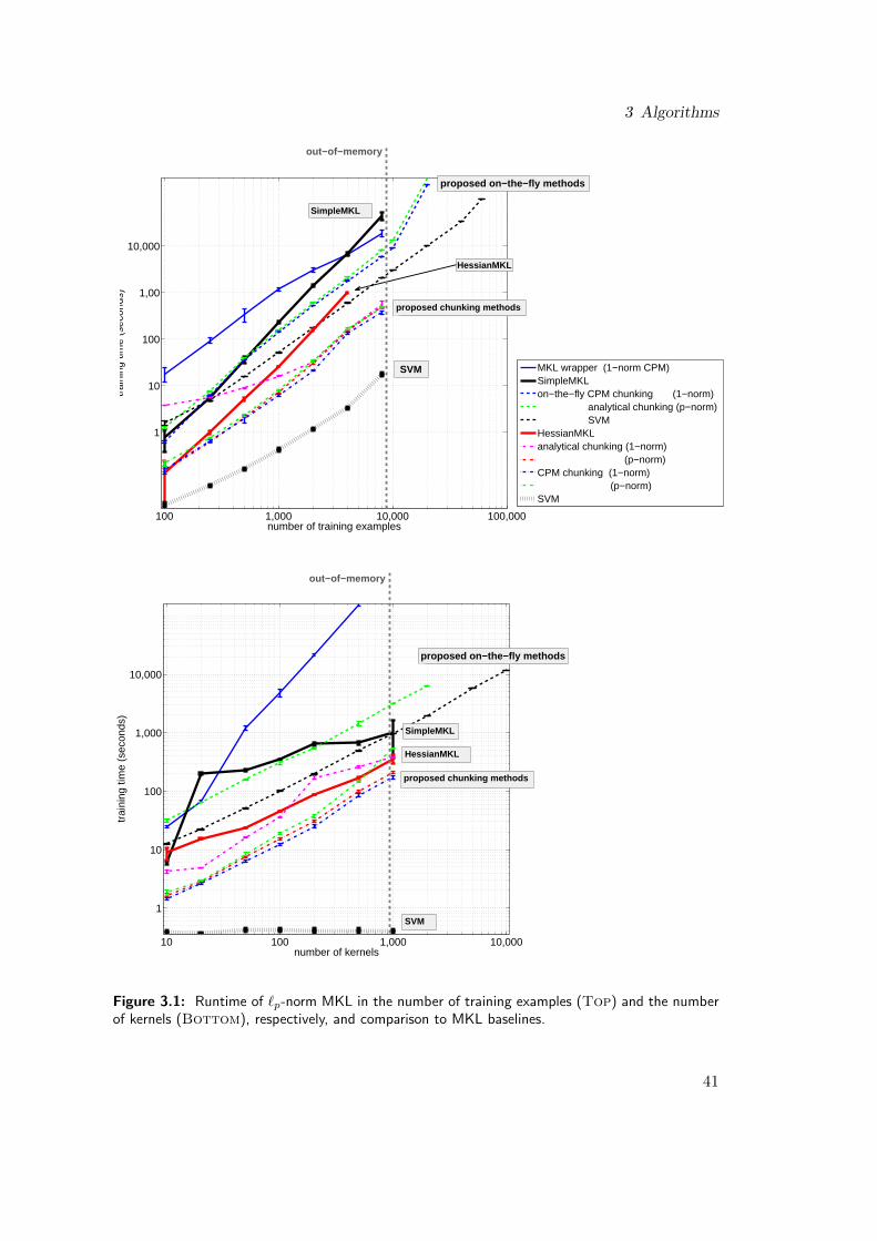
3 Algorithms
100 1,000 10,000 100,000
1
10
100
1,00
10,000
number of training examples
trai
ning
tim
e (s
econ
ds)
MKL wrapper (1−norm CPM)SimpleMKLon−the−fly CPM chunking (1−norm) analytical chunking (p−norm) SVM HessianMKLanalytical chunking (1−norm) (p−norm)CPM chunking (1−norm) (p−norm)SVM
proposed chunking methods
SVM
proposed on−the−fly methods
HessianMKL
SimpleMKL
out−of−memory
10 100 1,000 10,000
1
10
100
1,000
10,000
number of kernels
trai
ning
tim
e (s
econ
ds)
SVM
proposed on−the−fly methods
out−of−memory
proposed chunking methods
HessianMKL
SimpleMKL
Figure 3.1: Runtime of `p-norm MKL in the number of training examples (Top) and the numberof kernels (Bottom), respectively, and comparison to MKL baselines.
41
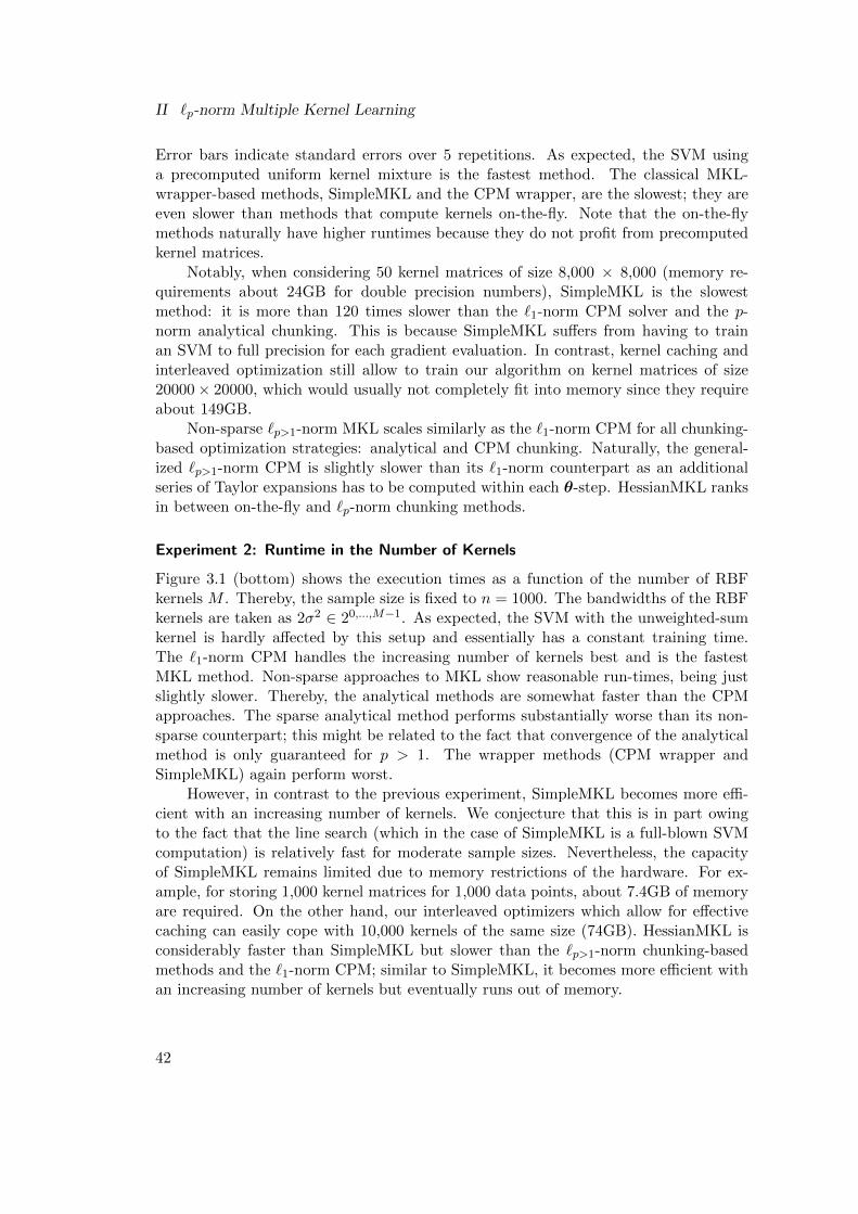
II `p-norm Multiple Kernel Learning
Error bars indicate standard errors over 5 repetitions. As expected, the SVM usinga precomputed uniform kernel mixture is the fastest method. The classical MKL-wrapper-based methods, SimpleMKL and the CPM wrapper, are the slowest; they areeven slower than methods that compute kernels on-the-fly. Note that the on-the-flymethods naturally have higher runtimes because they do not profit from precomputedkernel matrices.
Notably, when considering 50 kernel matrices of size 8,000 × 8,000 (memory re-quirements about 24GB for double precision numbers), SimpleMKL is the slowestmethod: it is more than 120 times slower than the `1-norm CPM solver and the p-norm analytical chunking. This is because SimpleMKL suffers from having to trainan SVM to full precision for each gradient evaluation. In contrast, kernel caching andinterleaved optimization still allow to train our algorithm on kernel matrices of size20000× 20000, which would usually not completely fit into memory since they requireabout 149GB.
Non-sparse `p>1-norm MKL scales similarly as the `1-norm CPM for all chunking-based optimization strategies: analytical and CPM chunking. Naturally, the general-ized `p>1-norm CPM is slightly slower than its `1-norm counterpart as an additionalseries of Taylor expansions has to be computed within each θ-step. HessianMKL ranksin between on-the-fly and `p-norm chunking methods.
Experiment 2: Runtime in the Number of Kernels
Figure 3.1 (bottom) shows the execution times as a function of the number of RBFkernels M . Thereby, the sample size is fixed to n = 1000. The bandwidths of the RBFkernels are taken as 2σ2 ∈ 20,...,M−1. As expected, the SVM with the unweighted-sumkernel is hardly affected by this setup and essentially has a constant training time.The `1-norm CPM handles the increasing number of kernels best and is the fastestMKL method. Non-sparse approaches to MKL show reasonable run-times, being justslightly slower. Thereby, the analytical methods are somewhat faster than the CPMapproaches. The sparse analytical method performs substantially worse than its non-sparse counterpart; this might be related to the fact that convergence of the analyticalmethod is only guaranteed for p > 1. The wrapper methods (CPM wrapper andSimpleMKL) again perform worst.
However, in contrast to the previous experiment, SimpleMKL becomes more effi-cient with an increasing number of kernels. We conjecture that this is in part owingto the fact that the line search (which in the case of SimpleMKL is a full-blown SVMcomputation) is relatively fast for moderate sample sizes. Nevertheless, the capacityof SimpleMKL remains limited due to memory restrictions of the hardware. For ex-ample, for storing 1,000 kernel matrices for 1,000 data points, about 7.4GB of memoryare required. On the other hand, our interleaved optimizers which allow for effectivecaching can easily cope with 10,000 kernels of the same size (74GB). HessianMKL isconsiderably faster than SimpleMKL but slower than the `p>1-norm chunking-basedmethods and the `1-norm CPM; similar to SimpleMKL, it becomes more efficient withan increasing number of kernels but eventually runs out of memory.
42
3 Algorithms
Overall, the proposed chunking-based optimization strategies (analytic and CPM)achieve a speedup of up to one and two orders of magnitude over HessianMKL andSimpleMKL, respectively. Using efficient kernel caching, they allow for truly large-scalemultiple kernel learning—well beyond the limits imposed by having to precompute andstore the complete kernel matrices.
3.5 Summary and Discussion
In this chapter, we derived two efficient algorithms for solving the `p-norm MKL op-timization problem. Both algorithms were, for the sake of performance, implementedin C++ and made available as a part of the open source machine learning toolboxSHOGUN (Sonnenburg et al., 2010), which also contains interfaces to MATLAB, Oc-tave, Phyton, and R. In our computational experiments, we found these large-scaleoptimization algorithms allowing us to deal with ten thousands of data points andthousands of kernels at the same time, as demonstrated on the MNIST data set. Wecompared our algorithms to the state-of-the-art in MKL research, namely HessianMKL(Chapelle and Rakotomamonjy, 2008) and SimpleMKL (Rakotomamonjy et al., 2008),and found ours to be up to two magnitudes faster. Both algorithms are based on thealternative, wrapper-based `p-norm MKL formulation (Problem II.4) in contrast to theoriginal problem (Problem II.3).
The first algorithm, the analytical wrapper, consists of an iterate 2-step proce-dure, alternatingly performing the analytical MKL step and calling an SVM solver(to this end, both, SVMlight and LIBSVM, are implemented in SHOGUN). Clearly,AnalyticalMKL is even simpler than SimpleMKL since the latter requires a heuristicline search in the MKL step. We showed AnalyticalMKL being provably convergent,using the usual regularity assumptions. The second algorithm, the analytical chunking,is directly integrated into the SVM light code (i.e., the MKL step is called after eachchunking iteration), allowing for truly large-scale MKL.
We remark that the proposed algorithms can, in particular, be used to optimize theclassical `p=1-norm MKL formulation. However, we found the algorithms in some casesto converge considerably faster in the non-sparse case p > 1, where the smoothnessof the objective can be exploited. Considering the gain in prediction accuracy that isalso achieved by `p>1-norm MKL, established later in this dissertation, this might beremarkable. Note that we also wrote scripts completely automating the whole processfrom training over model selection to evaluation. Currently, MKL can be trained andvalidated by a single line of MATLAB code including random subsampling, modelsearch for the optimal parameters C and p, and collection of results. Our software isfreely available under the GPL license. We also remark that another fast algorithmbased on cutting planes is described in Appendix D. We found this algorithm to beeven faster in some cases but it requires a commercial QCQP solver so that it cannotbe released under the GPL license.
Finally, we note that performing MKL with 1,000 precomputed kernel matrices of
43

II `p-norm Multiple Kernel Learning
size 1,000 × 1,000 requires less than 3 minutes for the chunking methods. This suggeststo focus future research efforts rather on improving the accuracy of MKL models ratherthan accelerating the optimization algorithms.
44
4 Theoretical Analysis
4 Theoretical Analysis
In this chapter, we derive upper bounds on the global and local Rademacher com-plexities of `p-norm MKL, from which we deduce excess risk bounds that achieve fast
convergence rates of the order O(n−α
1+α ), where α is the minimum eigenvalue decay rate
of the individual kernels (previous bounds for `p-norm MKL only achieved O(n−12 )).
We also give a lower bound that, up to constants, matches the upper bounds, showingthat our results are tight. Finally, the generalization performance of `p-norm MKL, asguaranteed by the excess risk bound, is studied for varying values of p, shedding lighton why learning kernels can help performance. This chapter is based on mathematicalpreliminaries introduced in Appendix A.
The main contributions in this chapter are the following:
• We derive an upper bound on the local Rademacher complexity of `p-norm multiplekernel learning that yields an excess risk bound achieving fast convergence rates, whileprevious approaches only yielded slow rates.
• We also prove a lower bound that matches the upper one, showing that our result istight.
• As a byproduct, we extend a previous upper bound of Cortes et al. (2010a) on theglobal Rademacher complexity to the full range of p ∈ [1,∞], yet presenting a sub-stantially easier proof and improved constants.
• We exemplarily evaluate the bound for several scenarios that differ in the soft sparsityof the underlying Bayes hypothesis, shedding light on why learning kernels can helpperformance.
Parts of this chapter are based on:
M. Kloft and G. Blanchard. The local Rademacher Complexity of Multiple KernelLearning. ArXiv preprint 1103.0790v1. Submitted to Journal of Machine LearningResearch (JMLR) , Mar 2011.
A short version has been submitted to Twenty-Fifth Annual Conference on NeuralInformation Processing Systems (NIPS 2011), Jun 2011.
Notation
For the upcoming analysis it is convenient to view MKL as an empirical minimizationalgorithm acting on the hypothesis class
Hp,D,M =fw : x 7→ 〈w, φ(x)〉
∣∣ w = (w(1), . . . ,w(M)), ‖w‖2,p ≤ D
(4.1)
(if D or M are clear from the context, we sometimes denote Hp = Hp,D = Hp,D,M ).This is equivalent to the original formulation in Problem 2.1, where we viewed MKL asregularized risk minimization problem. To see the equivalence between the regulariza-tion and hypothesis-class views, note that we can equivalently translate the Tikhonov-regularized MKL problem in an Ivanov-regularized problem by applying Lemma B.1(presented in Appendix B).
45
II `p-norm Multiple Kernel Learning
Furthermore, let P be a probability measure on X independently generating thedata x1, . . . , xn and denote by E the corresponding expectation operator. Note that forx ∼ P we can view φ(x) and φm(x) as random variables taking values in the Hilbertspaces H and Hm, respectively. Correspondingly, we will work with covariance opera-tors in Hilbert spaces. In a finite dimensional vector space, the (uncentered) covarianceoperator can be defined in the usual vector/matrix notation as Eφ(x)φ(x)>. Since weare working with potentially infinite-dimensional vector spaces, instead of φ(x)φ(x)> wewill use the tensor notation φ(x)⊗φ(x) ∈ HS(H), which is a Hilbert-Schmidt operatorH 7→ H defined as (φ(x) ⊗ φ(x))u = 〈φ(x),u〉φ(x). The space HS(H) of Hilbert-Schmidt operators on H is itself a Hilbert space, and the expectation Eφ(x) ⊗ φ(x)is well-defined and belongs to HS(H) as soon as E ‖φ(x)‖2 is finite, which will alwaysbe assumed as such (as a matter of fact, we will often assume that ‖φ(x)‖ is boundeda.s.). We denote by J = Eφ(x) ⊗ φ(x) and Jm = Eφm(x) ⊗ φm(x) the uncenteredcovariance operators corresponding to variables φ(x) and φm(x), respectively; it holdsthat tr(J) = E ‖φ(x)‖22 and tr(Jm) = E ‖φm(x)‖22.
4.1 Global Rademacher Complexity
We first review global Rademacher complexities (GRC) in multiple kernel learning. Letx1, . . . , xn be an i.i.d. sample drawn from P . The global Rademacher complexity isdefined as R(Hp) = E supfw∈Hp〈w,
1n
∑ni=1 σiφ(xi)〉, where (σi)1≤i≤n is an i.i.d. family
(independent of φ(xi)) of Rademacher variables (random signs). Its empirical counter-part is denoted by R(Hp) = E
[R(Hp)
∣∣x1, . . . , xn] = Eσ supfw∈Hp〈w,1n
∑ni=1 σiφ(xi)〉.
The interest in the global Rademacher complexity comes from the fact that, if known, itcan be used to bound the generalization error (Koltchinskii, 2001; Bartlett and Mendel-son, 2002); see Appendix A.
In the recent paper of Cortes et al. (2010a) it was shown, using a combinatorial argu-ment, that the empirical version of the global Rademacher complexity can be boundedas
R(Hp) ≤D
n
√cp∗∥∥∥(tr(Km)
)Mm=1
∥∥∥p∗2
(for p ∈ [1, 2] and p∗ being an integer)
where c = 2322 . We will now show a quite short proof of this result (extending it to
the whole range p ∈ [1,∞]) and then present a novel bound on the population versionof the GRC. The proof presented here is based on the Khintchine-Kahane inequality(Kahane, 1985) using the constants taken from Lemma 3.3.1 and Proposition 3.4.1 inKwapien and Woyczynski (1992).
Lemma 4.1 (Khintchine-Kahane inequality). Let v1, . . . ,vM ∈ H. Then, forany q ≥ 1, it holds
Eσ∥∥ n∑i=1
σivi∥∥q2≤(c
n∑i=1
∥∥vi∥∥22) q2 ,where c = max(1, p∗ − 1). In particular, the result holds for c = p∗.
46
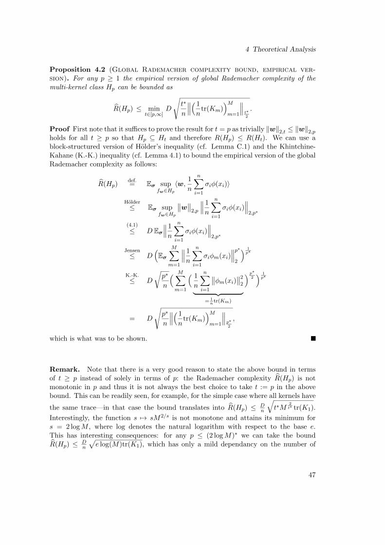
4 Theoretical Analysis
Proposition 4.2 (Global Rademacher complexity bound, empirical ver-sion). For any p ≥ 1 the empirical version of global Rademacher complexity of themulti-kernel class Hp can be bounded as
R(Hp) ≤ mint∈[p,∞]
D
√t∗
n
∥∥∥( 1
ntr(Km)
)Mm=1
∥∥∥t∗2
.
Proof First note that it suffices to prove the result for t = p as trivially ‖w‖2,t ≤ ‖w‖2,pholds for all t ≥ p so that Hp ⊆ Ht and therefore R(Hp) ≤ R(Ht). We can use ablock-structured version of Holder’s inequality (cf. Lemma C.1) and the Khintchine-Kahane (K.-K.) inequality (cf. Lemma 4.1) to bound the empirical version of the globalRademacher complexity as follows:
R(Hp)def.= Eσ sup
fw∈Hp〈w, 1
n
n∑i=1
σiφ(xi)〉
Holder≤ Eσ sup
fw∈Hp
∥∥w∥∥2,p
∥∥∥ 1
n
n∑i=1
σiφ(xi)∥∥∥2,p∗
(4.1)
≤ D Eσ∥∥∥ 1
n
n∑i=1
σiφ(xi)∥∥∥2,p∗
Jensen≤ D
(Eσ
M∑m=1
∥∥∥ 1
n
n∑i=1
σiφm(xi)∥∥∥p∗2
) 1p∗
K.-K.≤ D
√p∗
n
( M∑m=1
( 1
n
n∑i=1
∥∥φm(xi)∥∥22︸ ︷︷ ︸
= 1ntr(Km)
) p∗2) 1p∗
= D
√p∗
n
∥∥∥( 1
ntr(Km)
)Mm=1
∥∥∥p∗2
,
which is what was to be shown.
Remark. Note that there is a very good reason to state the above bound in termsof t ≥ p instead of solely in terms of p: the Rademacher complexity R(Hp) is notmonotonic in p and thus it is not always the best choice to take t := p in the abovebound. This can be readily seen, for example, for the simple case where all kernels have
the same trace—in that case the bound translates into R(Hp) ≤ Dn
√t∗M
2t∗ tr(K1).
Interestingly, the function s 7→ sM2/s is not monotone and attains its minimum fors = 2 logM , where log denotes the natural logarithm with respect to the base e.This has interesting consequences: for any p ≤ (2 logM)∗ we can take the boundR(Hp) ≤ D
n
√e log(M)tr(K1), which has only a mild dependancy on the number of
47
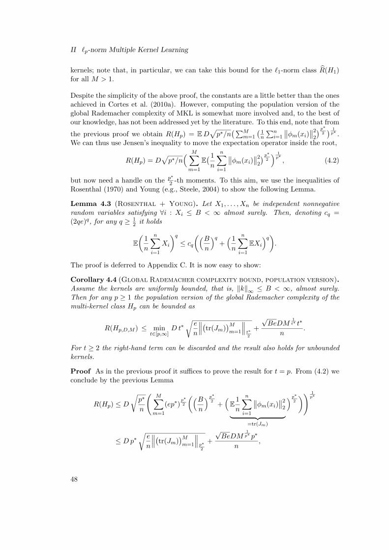
II `p-norm Multiple Kernel Learning
kernels; note that, in particular, we can take this bound for the `1-norm class R(H1)for all M > 1.
Despite the simplicity of the above proof, the constants are a little better than the onesachieved in Cortes et al. (2010a). However, computing the population version of theglobal Rademacher complexity of MKL is somewhat more involved and, to the best ofour knowledge, has not been addressed yet by the literature. To this end, note that from
the previous proof we obtain R(Hp) = ED√p∗/n
(∑Mm=1
(1n
∑ni=1
∥∥φm(xi)∥∥22
) p∗2) 1p∗ .
We can thus use Jensen’s inequality to move the expectation operator inside the root,
R(Hp) = D√p∗/n
( M∑m=1
E( 1
n
n∑i=1
∥∥φm(xi)∥∥22
) p∗2
) 1p∗, (4.2)
but now need a handle on the p∗
2 -th moments. To this aim, we use the inequalities ofRosenthal (1970) and Young (e.g., Steele, 2004) to show the following Lemma.
Lemma 4.3 (Rosenthal + Young). Let X1, . . . , Xn be independent nonnegativerandom variables satisfying ∀i : Xi ≤ B < ∞ almost surely. Then, denoting cq =(2qe)q, for any q ≥ 1
2 it holds
E(
1
n
n∑i=1
Xi
)q≤ cq
((Bn
)q+( 1
n
n∑i=1
EXi
)q).
The proof is deferred to Appendix C. It is now easy to show:
Corollary 4.4 (Global Rademacher complexity bound, population version).Assume the kernels are uniformly bounded, that is, ‖k‖∞ ≤ B < ∞, almost surely.Then for any p ≥ 1 the population version of the global Rademacher complexity of themulti-kernel class Hp can be bounded as
R(Hp,D,M ) ≤ mint∈[p,∞]
D t∗√e
n
∥∥∥(tr(Jm))Mm=1
∥∥∥t∗2
+
√BeDM
1t∗ t∗
n.
For t ≥ 2 the right-hand term can be discarded and the result also holds for unboundedkernels.
Proof As in the previous proof it suffices to prove the result for t = p. From (4.2) weconclude by the previous Lemma
R(Hp) ≤ D√p∗
n
(M∑m=1
(ep∗)p∗2
((Bn
) p∗2
+(E
1
n
n∑i=1
∥∥φm(xi)∥∥22︸ ︷︷ ︸
=tr(Jm)
) p∗2
)) 1p∗
≤ Dp∗√e
n
∥∥∥(tr(Jm))Mm=1
∥∥∥p∗2
+
√BeDM
1p∗ p∗
n,
48
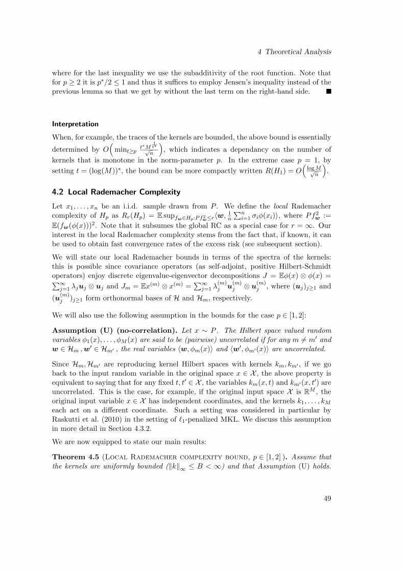
4 Theoretical Analysis
where for the last inequality we use the subadditivity of the root function. Note thatfor p ≥ 2 it is p∗/2 ≤ 1 and thus it suffices to employ Jensen’s inequality instead of theprevious lemma so that we get by without the last term on the right-hand side.
Interpretation
When, for example, the traces of the kernels are bounded, the above bound is essentially
determined by O(
mint≥pt∗M
1t∗√n
), which indicates a dependancy on the number of
kernels that is monotone in the norm-parameter p. In the extreme case p = 1, by
setting t = (log(M))∗, the bound can be more compactly written R(H1) = O(logM√
n
).
4.2 Local Rademacher Complexity
Let x1, . . . , xn be an i.i.d. sample drawn from P . We define the local Rademachercomplexity of Hp as Rr(Hp) = E supfw∈Hp:Pf2w≤r〈w,
1n
∑ni=1 σiφ(xi)〉, where Pf2w :=
E(fw(φ(x)))2. Note that it subsumes the global RC as a special case for r = ∞. Ourinterest in the local Rademacher complexity stems from the fact that, if known, it canbe used to obtain fast convergence rates of the excess risk (see subsequent section).
We will state our local Rademacher bounds in terms of the spectra of the kernels:this is possible since covariance operators (as self-adjoint, positive Hilbert-Schmidtoperators) enjoy discrete eigenvalue-eigenvector decompositions J = Eφ(x) ⊗ φ(x) =∑∞
j=1 λjuj ⊗ uj and Jm = Ex(m) ⊗ x(m) =∑∞
j=1 λ(m)j u
(m)j ⊗ u(m)
j , where (uj)j≥1 and
(u(m)j )j≥1 form orthonormal bases of H and Hm, respectively.
We will also use the following assumption in the bounds for the case p ∈ [1, 2]:
Assumption (U) (no-correlation). Let x ∼ P . The Hilbert space valued randomvariables φ1(x), . . . , φM (x) are said to be (pairwise) uncorrelated if for any m 6= m′ andw ∈ Hm ,w′ ∈ Hm′ , the real variables 〈w, φm(x)〉 and 〈w′, φm′(x)〉 are uncorrelated.
Since Hm,Hm′ are reproducing kernel Hilbert spaces with kernels km, km′ , if we goback to the input random variable in the original space x ∈ X , the above property isequivalent to saying that for any fixed t, t′ ∈ X , the variables km(x, t) and km′(x, t
′) areuncorrelated. This is the case, for example, if the original input space X is RM , theoriginal input variable x ∈ X has independent coordinates, and the kernels k1, . . . , kMeach act on a different coordinate. Such a setting was considered in particular byRaskutti et al. (2010) in the setting of `1-penalized MKL. We discuss this assumptionin more detail in Section 4.3.2.
We are now equipped to state our main results:
Theorem 4.5 (Local Rademacher complexity bound, p ∈ [1, 2] ). Assume thatthe kernels are uniformly bounded (‖k‖∞ ≤ B < ∞) and that Assumption (U) holds.
49
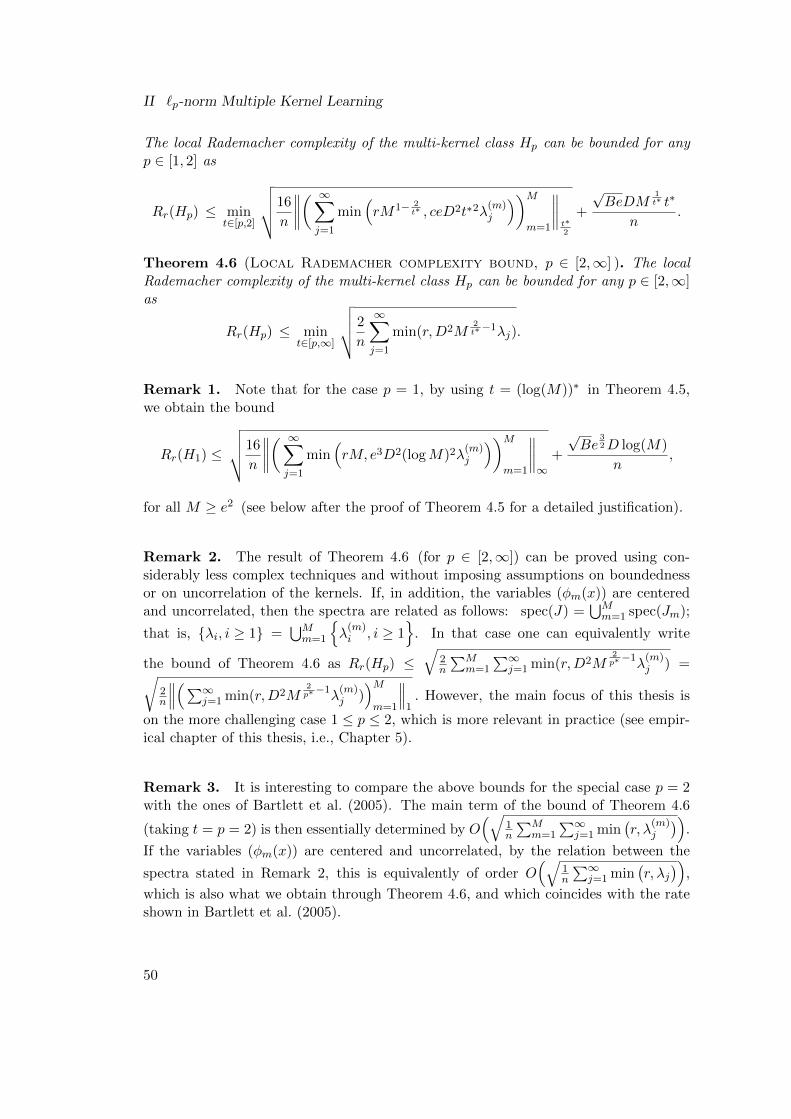
II `p-norm Multiple Kernel Learning
The local Rademacher complexity of the multi-kernel class Hp can be bounded for anyp ∈ [1, 2] as
Rr(Hp) ≤ mint∈[p,2]
√√√√16
n
∥∥∥∥( ∞∑j=1
min(rM1− 2
t∗ , ceD2t∗2λ(m)j
))Mm=1
∥∥∥∥t∗2
+
√BeDM
1t∗ t∗
n.
Theorem 4.6 (Local Rademacher complexity bound, p ∈ [2,∞] ). The localRademacher complexity of the multi-kernel class Hp can be bounded for any p ∈ [2,∞]as
Rr(Hp) ≤ mint∈[p,∞]
√√√√ 2
n
∞∑j=1
min(r,D2M2t∗−1λj).
Remark 1. Note that for the case p = 1, by using t = (log(M))∗ in Theorem 4.5,we obtain the bound
Rr(H1) ≤
√√√√16
n
∥∥∥∥( ∞∑j=1
min(rM, e3D2(logM)2λ
(m)j
))Mm=1
∥∥∥∥∞
+
√Be
32D log(M)
n,
for all M ≥ e2 (see below after the proof of Theorem 4.5 for a detailed justification).
Remark 2. The result of Theorem 4.6 (for p ∈ [2,∞]) can be proved using con-siderably less complex techniques and without imposing assumptions on boundednessor on uncorrelation of the kernels. If, in addition, the variables (φm(x)) are centeredand uncorrelated, then the spectra are related as follows: spec(J) =
⋃Mm=1 spec(Jm);
that is, λi, i ≥ 1 =⋃Mm=1
λ(m)i , i ≥ 1
. In that case one can equivalently write
the bound of Theorem 4.6 as Rr(Hp) ≤√
2n
∑Mm=1
∑∞j=1 min(r,D2M
2p∗−1λ
(m)j ) =√
2n
∥∥∥(∑∞j=1 min(r,D2M2p∗−1λ
(m)j )
)Mm=1
∥∥∥1. However, the main focus of this thesis is
on the more challenging case 1 ≤ p ≤ 2, which is more relevant in practice (see empir-ical chapter of this thesis, i.e., Chapter 5).
Remark 3. It is interesting to compare the above bounds for the special case p = 2with the ones of Bartlett et al. (2005). The main term of the bound of Theorem 4.6
(taking t = p = 2) is then essentially determined by O(√
1n
∑Mm=1
∑∞j=1 min
(r, λ
(m)j
)).
If the variables (φm(x)) are centered and uncorrelated, by the relation between the
spectra stated in Remark 2, this is equivalently of order O(√
1n
∑∞j=1 min
(r, λj
)),
which is also what we obtain through Theorem 4.6, and which coincides with the rateshown in Bartlett et al. (2005).
50
4 Theoretical Analysis
Proof of Theorem 4.5. The proof is based on first relating the complexity of theclass Hp to its centered counterpart, i.e., where all functions fw ∈ Hp are centeredaround their expected value. Then we compute the complexity of the centered classby decomposing the complexity into blocks, applying the no-correlation assumption,and using the inequalities of Holder and Rosenthal. Then we relate it back to theoriginal class, which, in the final step, we relate to a bound involving the truncationof the particular spectra of the kernels. Note that it suffices to prove the result fort = p as trivially ‖w‖2,t ≤ ‖w‖2,p holds for all t ≥ p so that Hp ⊆ Ht and thereforeRr(Hp) ≤ Rr(Ht).
Step 1: Relating the original class with the centered class. In orderto exploit the no-correlation assumption, we will work in large parts of the proof withthe centered class Hp =
fw∣∣ ‖w‖2,p ≤ D
, wherein fw : x 7→ 〈w, φ(x)〉, and φ(x) :=
φ(x)−Eφ(x). We start the proof by noting that fw(x) = fw(x)−〈w,Eφ(x)〉 = fw(x)−E 〈w, φ(x)〉 = fw(φ(x)) − Efw(φ(x)), so that, by the bias-variance decomposition, itholds that
Pf2w = Efw(x)2 = E (fw(x)− Efw(x))2 + (Efw(φ(x)))2 = P f2w +(Pfw
)2. (4.3)
Furthermore, we note that by Jensen’s inequality
∥∥Eφ(x)∥∥2,p∗
=
( M∑m=1
∥∥Eφm(x)∥∥p∗2
) 1p∗
=
( M∑m=1
⟨Eφm(x),Eφm(x)
⟩ p∗2
) 1p∗
Jensen≤
( M∑m=1
E⟨φm(x), φm(x)
⟩ p∗2
) 1p∗
=
√∥∥∥(tr(Jm))Mm=1
∥∥∥p∗2
(4.4)
so that we can express the complexity of the centered class in terms of the uncenteredone as follows:
Rr(Hp) = E supfw∈Hp,Pf2w≤r
⟨w,
1
n
n∑i=1
σiφ(xi)⟩
≤ E supfw∈Hp,Pf2w≤r
⟨w,
1
n
n∑i=1
σiφ(xi)⟩
+ E supfw∈Hp,Pf2w≤r
⟨w,
1
n
n∑i=1
σiEφ(x)⟩.
Concerning the first term of the above upper bound, using (4.3) we have P f2w ≤ Pf2w,and thus
E supfw∈Hp,Pf2w≤r
⟨w,
1
n
n∑i=1
σiφ(xi)⟩≤ E sup
fw∈Hp,P f2w≤r
⟨w,
1
n
n∑i=1
σiφ(xi)⟩
= Rr(Hp).
51
II `p-norm Multiple Kernel Learning
Now to bound the second term, we write
E supfw∈Hp,Pf2w≤r
⟨w,
1
n
n∑i=1
σiEφ(x)⟩
= E
∣∣∣∣∣ 1nn∑i=1
σi
∣∣∣∣∣ supfw∈Hp,Pf2w≤r
〈w,Eφ(x)〉
≤ supfw∈Hp,Pf2w≤r
⟨w,Eφ(x)
⟩E
(1
n
n∑i=1
σi
)2 1
2
=√n supfw∈Hp,Pf2w≤r
〈w,Eφ(x)〉 .
We finally observe
〈w,Eφ(x)〉Holder≤ ‖w‖2,p ‖Eφ(x)‖2,p∗
(4.4)
≤ ‖w‖2,p
√∥∥(tr(Jm))Mm=1
∥∥p∗2
as well as
〈w,Eφ(x)〉 = Efw(x) ≤√Pf2w .
Putting the above steps together, we obtain as a result
Rr(Hp) ≤ Rr(Hp) + n−12 min
(√r,D
√∥∥(tr(Jm))Mm=1
∥∥p∗2
). (4.5)
This shows that, at the expense of the additional summand on the right-hand side, wecan work with the centered class instead of the uncentered one.
Step 2: Bounding the complexity of the centered class. Since the (cen-tered) covariance operator Eφm(x)⊗ φm(x) is also a self-adjoint Hilbert-Schmidt oper-ator on Hm, there exists an eigendecomposition
Eφm(x)⊗ φm(x) =
∞∑j=1
λ(m)j u
(m)j ⊗ u(m)
j , (4.6)
wherein (u(m)j )j≥1 is an orthogonal basis of Hm. Furthermore, the no-correlation as-
sumption (U) entails Eφl(x)⊗ φm(x) = 0 for all l 6= m. As a consequence,
P f2w = E(fw(x))2 = E( M∑m=1
⟨wm, φm(x)
⟩)2=
M∑l,m=1
⟨wl,
(Eφl(x)⊗ φm(x)
)wm
⟩(U)=
M∑m=1
⟨wm,
(Eφm(x)⊗ φm(x)
)wm
⟩=
M∑m=1
∞∑j=1
λ(m)j
⟨wm, u
(m)j
⟩2(4.7)
52
4 Theoretical Analysis
and, for all j and m,
E⟨ 1
n
n∑i=1
σiφm(xi), u(m)j
⟩2= E
1
n2
n∑i,l=1
σiσl
⟨φm(xi), u
(m)j
⟩⟨φm(xl), u
(m)j
⟩σ i.i.d.
= E1
n2
n∑i=1
⟨φm(xi), u
(m)j
⟩2=
1
n
⟨u(m)j ,
( 1
n
n∑i=1
E φm(xi)⊗ φm(xi)︸ ︷︷ ︸=Eφm(x)⊗φm(x)
)u(m)j
⟩
=λ(m)j
n. (4.8)
Let now h1, . . . , hM be arbitrary nonnegative integers. We can express the localRademacher complexity in terms of the eigendecompositon (4.6) as follows
Rr(Hp)
= E supfw∈Hp:P f2w≤r
⟨w,
1
n
n∑i=1
σiφ(xi)⟩
= E supfw∈Hp:P f2w≤r
⟨(w(m)
)Mm=1
,( 1
n
n∑i=1
σiφm(xi))Mm=1
⟩
≤ E supP f2w≤r
⟨ ( hm∑j=1
√λ(m)j 〈w
(m), u(m)j 〉u
(m)j
)Mm=1
,
( hm∑j=1
√λ(m)j
−1〈 1n
n∑i=1
σiφm(xi), u(m)j 〉u
(m)j
)Mm=1
⟩+ E sup
fw∈Hp
⟨w,( ∞∑j=hm+1
〈 1n
n∑i=1
σiφm(xi), u(m)j 〉u
(m)j
)Mm=1
⟩
C.-S., Jensen≤ sup
P f2w≤r
[ M∑m=1
hm∑j=1
λ(m)j 〈w
(m), u(m)j 〉
2
12
×
M∑m=1
hm∑j=1
(λ(m)j
)−1E⟨ 1
n
n∑i=1
σiφm(xi), u(m)j
⟩2 12 ]
+ E supfw∈Hp
⟨w,( ∞∑j=hm+1
〈 1n
n∑i=1
σiφm(xi), u(m)j 〉u
(m)j
)Mm=1
⟩
53
II `p-norm Multiple Kernel Learning
so that (4.7) and (4.8) yield
Rr(Hp)
(4.7), (4.8)
≤
√r∑M
m=1 hmn
+ E supfw∈Hp
⟨w,( ∞∑j=hm+1
〈 1n
n∑i=1
σiφm(xi), u(m)j 〉u
(m)j
)Mm=1
⟩Holder≤
√r∑M
m=1 hmn
+D E∥∥∥∥( ∞∑
j=hm+1
〈 1n
n∑i=1
σiφm(xi), u(m)j 〉u
(m)j
)Mm=1
∥∥∥∥2,p∗
.
(4.9)
Step 3: Khintchine-Kahane’s and Rosenthal’s inequalities. We can nowuse the Khintchine-Kahane (K.-K.) inequality (see Lemma 4.1 in Appendix C) to fur-ther bound the right term in the above expression as follows
E∥∥∥∥( ∞∑
j=hm+1
〈 1n
n∑i=1
σiφm(xi), u(m)j 〉u
(m)j
)Mm=1
∥∥∥∥2,p∗
Jensen≤ E
( M∑m=1
Eσ∥∥∥∥ ∞∑j=hm+1
〈 1n
n∑i=1
σiφm(xi), u(m)j 〉u
(m)j
∥∥∥∥p∗Hm
) 1p∗
K.-K.≤
√p∗
nE( M∑m=1
( ∞∑j=hm+1
1
n
n∑i=1
〈φm(xi), u(m)j 〉
2) p∗
2
) 1p∗
Jensen≤
√p∗
n
( M∑m=1
E( ∞∑j=hm+1
1
n
n∑i=1
〈φm(xi), u(m)j 〉
2) p∗
2
) 1p∗
.
Note that for p ≥ 2 it holds that p∗/2 ≤ 1, and thus it suffices to employ Jensen’sinequality once again in order to move the expectation operator inside the inner term.In the general case, we need a handle on the p∗
2 -th moments and to this end employ
54
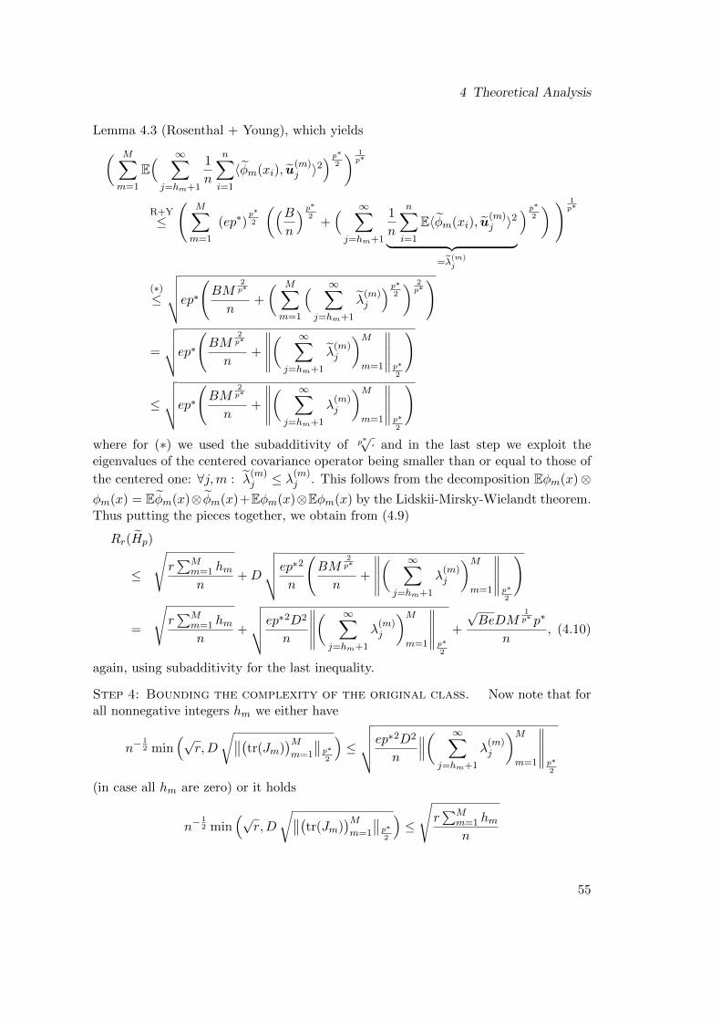
4 Theoretical Analysis
Lemma 4.3 (Rosenthal + Young), which yields( M∑m=1
E( ∞∑j=hm+1
1
n
n∑i=1
〈φm(xi), u(m)j 〉
2) p∗
2
) 1p∗
R+Y≤
(M∑m=1
(ep∗)p∗2
((Bn
) p∗2
+( ∞∑j=hm+1
1
n
n∑i=1
E〈φm(xi), u(m)j 〉
2
︸ ︷︷ ︸=λ
(m)j
) p∗2
) ) 1p∗
(∗)≤
√√√√ep∗
(BM
2p∗
n+
( M∑m=1
( ∞∑j=hm+1
λ(m)j
) p∗2
) 2p∗)
=
√√√√ep∗
(BM
2p∗
n+
∥∥∥∥∥( ∞∑j=hm+1
λ(m)j
)Mm=1
∥∥∥∥∥p∗2
)
≤
√√√√ep∗
(BM
2p∗
n+
∥∥∥∥∥( ∞∑j=hm+1
λ(m)j
)Mm=1
∥∥∥∥∥p∗2
)
where for (∗) we used the subadditivity of p∗√· and in the last step we exploit the
eigenvalues of the centered covariance operator being smaller than or equal to those of
the centered one: ∀j,m : λ(m)j ≤ λ(m)
j . This follows from the decomposition Eφm(x)⊗φm(x) = Eφm(x)⊗ φm(x)+Eφm(x)⊗Eφm(x) by the Lidskii-Mirsky-Wielandt theorem.Thus putting the pieces together, we obtain from (4.9)
Rr(Hp)
≤
√r∑M
m=1 hmn
+D
√√√√ep∗2
n
(BM
2p∗
n+
∥∥∥∥∥( ∞∑j=hm+1
λ(m)j
)Mm=1
∥∥∥∥∥p∗2
)
=
√r∑M
m=1 hmn
+
√√√√ep∗2D2
n
∥∥∥∥∥( ∞∑j=hm+1
λ(m)j
)Mm=1
∥∥∥∥∥p∗2
+
√BeDM
1p∗ p∗
n, (4.10)
again, using subadditivity for the last inequality.
Step 4: Bounding the complexity of the original class. Now note that forall nonnegative integers hm we either have
n−12 min
(√r,D
√∥∥(tr(Jm))Mm=1
∥∥p∗2
)≤
√√√√ep∗2D2
n
∥∥∥( ∞∑j=hm+1
λ(m)j
)Mm=1
∥∥∥∥∥p∗2
(in case all hm are zero) or it holds
n−12 min
(√r,D
√∥∥(tr(Jm))Mm=1
∥∥p∗2
)≤
√r∑M
m=1 hmn
55
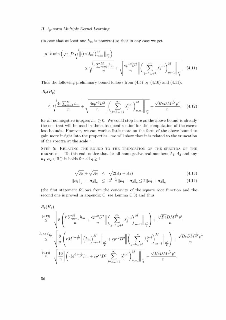
II `p-norm Multiple Kernel Learning
(in case that at least one hm is nonzero) so that in any case we get
n−12 min
(√r,D
√∥∥(tr(Jm))Mm=1
∥∥p∗2
)≤
√r∑M
m=1 hmn
+
√√√√ep∗2D2
n
∥∥∥∥∥( ∞∑j=hm+1
λ(m)j
)Mm=1
∥∥∥∥∥p∗2
. (4.11)
Thus the following preliminary bound follows from (4.5) by (4.10) and (4.11):
Rr(Hp)
≤
√4r∑M
m=1 hmn
+
√√√√4ep∗2D2
n
∥∥∥∥∥( ∞∑j=hm+1
λ(m)j
)Mm=1
∥∥∥∥∥p∗2
+
√BeDM
1p∗ p∗
n, (4.12)
for all nonnegative integers hm ≥ 0. We could stop here as the above bound is alreadythe one that will be used in the subsequent section for the computation of the excessloss bounds. However, we can work a little more on the form of the above bound togain more insight into the properties—we will show that it is related to the truncationof the spectra at the scale r.
Step 5: Relating the bound to the truncation of the spectra of thekernels. To this end, notice that for all nonnegative real numbers A1, A2 and anya1,a2 ∈ Rm+ it holds for all q ≥ 1
√A1 +
√A2 ≤
√2(A1 +A2) (4.13)
‖a1‖q + ‖a2‖q ≤ 21− 1
q ‖a1 + a2‖q ≤ 2 ‖a1 + a2‖q (4.14)
(the first statement follows from the concavity of the square root function and thesecond one is proved in appendix C; see Lemma C.3) and thus
Rr(Hp)
(4.13)
≤
√√√√√8
r∑Mm=1 hmn
+ep∗2D2
n
∥∥∥∥( ∞∑j=hm+1
λ(m)j
)Mm=1
∥∥∥∥p∗2
+
√BeDM
1p∗ p∗
n
`1-to-` p∗2
≤
√√√√√ 8
n
rM1− 2p∗
∥∥∥∥(hm)Mm=1
∥∥∥∥p∗2
+ ep∗2D2
∥∥∥∥( ∞∑j=hm+1
λ(m)j
)Mm=1
∥∥∥∥p∗2
+
√BeDM
1p∗ p∗
n
(4.14)
≤
√√√√16
n
∥∥∥∥(rM1− 2p∗ hm + ep∗2D2
∞∑j=hm+1
λ(m)j
)Mm=1
∥∥∥∥p∗2
+
√BeDM
1p∗ p∗
n,
56
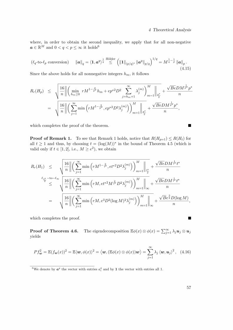
4 Theoretical Analysis
where, in order to obtain the second inequality, we apply that for all non-negativea ∈ RM and 0 < q < p ≤ ∞ it holds6
(`q-to-`p conversion) ‖a‖q = 〈1,aq〉1q
Holder≤
(‖1‖(p/q)∗ ‖a
q‖p/q)1/q
= M1q− 1p ‖a‖p .
(4.15)Since the above holds for all nonnegative integers hm, it follows
Rr(Hp) ≤
√√√√16
n
∥∥∥∥( minhm≥0
rM1− 2
p∗ hm + ep∗2D2
∞∑j=hm+1
λ(m)j
)Mm=1
∥∥∥∥p∗2
+
√BeDM
1p∗ p∗
n
=
√√√√16
n
∥∥∥∥( ∞∑j=1
min(rM
1− 2p∗ , ep∗2D2λ
(m)j
))Mm=1
∥∥∥∥p∗2
+
√BeDM
1p∗ p∗
n,
which completes the proof of the theorem.
Proof of Remark 1. To see that Remark 1 holds, notice that R(Hp=1) ≤ R(Ht) forall t ≥ 1 and thus, by choosing t = (log(M))∗ in the bound of Theorem 4.5 (which isvalid only if t ∈ [1, 2], i.e., M ≥ e2), we obtain
Rr(H1) ≤
√√√√16
n
∥∥∥∥( ∞∑j=1
min(rM1− 2
t∗ , et∗2D2λ(m)j
))Mm=1
∥∥∥∥t∗2
+
√BeDM
1t∗ t∗
n
` t∗2−to−`∞
≤
√√√√16
n
∥∥∥∥( ∞∑j=1
min(rM, et∗2M
2t∗D2λ
(m)j
))Mm=1
∥∥∥∥∞
+
√BeDM
1t∗ t∗
n
=
√√√√16
n
∥∥∥∥( ∞∑j=1
min(rM, e3D2(logM)2λ
(m)j
))Mm=1
∥∥∥∥∞
+
√Be
32D(logM)
n,
which completes the proof.
Proof of Theorem 4.6. The eigendecomposition Eφ(x)⊗ φ(x) =∑∞
j=1 λjuj ⊗ ujyields
Pf2w = E(fw(x))2 = E〈w, φ(x)〉2 =⟨w, (Eφ(x)⊗ φ(x))w
⟩=∞∑j=1
λj 〈w,uj〉2 , (4.16)
6We denote by aq the vector with entries aqi and by 1 the vector with entries all 1.
57
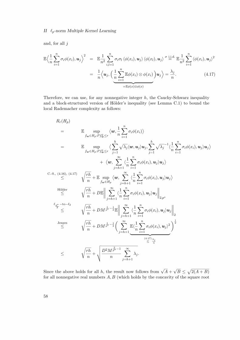
II `p-norm Multiple Kernel Learning
and, for all j
E⟨ 1
n
n∑i=1
σiφ(xi),uj
⟩2= E
1
n2
n∑i,l=1
σiσl 〈φ(xi),uj〉 〈φ(xl),uj〉σ i.i.d.
= E1
n2
n∑i=1
〈φ(xi),uj〉2
=1
n
⟨uj ,( 1
n
n∑i=1
Eφ(xi)⊗ φ(xi)︸ ︷︷ ︸=Eφ(x)⊗φ(x)
)uj
⟩=λjn. (4.17)
Therefore, we can use, for any nonnegative integer h, the Cauchy-Schwarz inequalityand a block-structured version of Holder’s inequality (see Lemma C.1) to bound thelocal Rademacher complexity as follows:
Rr(Hp)
= E supfw∈Hp:Pf2w≤r
⟨w,
1
n
n∑i=1
σiφ(xi)⟩
= E supfw∈Hp:Pf2w≤r
⟨ h∑j=1
√λj〈w,uj〉uj ,
h∑j=1
√λj−1〈 1
n
n∑i=1
σiφ(xi),uj〉uj⟩
+⟨w,
∞∑j=h+1
〈 1n
n∑i=1
σiφ(xi),uj〉uj⟩
C.-S., (4.16), (4.17)
≤√rh
n+ E sup
fw∈Hp
⟨w,
∞∑j=h+1
〈 1n
n∑i=1
σiφ(xi),uj〉uj⟩
Holder≤
√rh
n+DE
∥∥∥∥ ∞∑j=h+1
〈 1n
n∑i=1
σiφ(xi),uj〉uj∥∥∥∥2,p∗
` p∗2
−to−`2
≤√rh
n+DM
1p∗−
12E∥∥∥∥ ∞∑j=h+1
〈 1n
n∑i=1
σiφ(xi),uj〉uj∥∥∥∥2
Jensen≤
√rh
n+DM
1p∗−
12
( ∞∑j=h+1
E〈 1n
n∑i=1
σiφ(xi),uj〉2︸ ︷︷ ︸(4.17)
≤λjn
) 12
≤√rh
n+
√√√√D2M2p∗−1
n
∞∑j=h+1
λj .
Since the above holds for all h, the result now follows from√A +
√B ≤
√2(A+B)
for all nonnegative real numbers A,B (which holds by the concavity of the square root
58
4 Theoretical Analysis
function):
Rr(Hp) ≤
√√√√ 2
nmin
0≤h≤n
(rh+D2M
2p∗−1
∞∑j=h+1
λj
)=
√√√√ 2
n
∞∑j=1
min(r,D2M2p∗−1λj) .
4.2.1 Lower Bound
In this subsection we investigate the tightness of our bound on the local Rademachercomplexity of Hp. To derive a lower bound, we consider the particular case wherevariables φ1(x), . . . , φM (x) are i.i.d. For example, this happens if the original inputspace X is RM , the original input variable x ∈ X has i.i.d. coordinates, and the kernelsk1, . . . , kM are equal, but each acts on a different coordinate of x.
Lemma 4.7. Assume that the variables φ1(x), . . . , φM (x) are centered and identi-cally independently distributed. Then, the following lower bound holds for the localRademacher complexity of Hp for any p ≥ 1:
Rr(Hp,D,M ) ≥ RrM (H1,DM1/p∗ ,1).
Proof First note that, since the x(i) are centered and uncorrelated,
Pf2w =( M∑m=1
⟨wm, φm(x)
⟩)2=
M∑m=1
⟨wm, φm(x)
⟩2.
59
II `p-norm Multiple Kernel Learning
Now it follows
Rr(Hp,D,M ) = E sup
w:Pf2w≤r‖w‖2,p≤D
⟨w,
1
n
n∑i=1
σiφ(xi)⟩
= E sup
w:
∑Mm=1〈w(m),φm(x)〉2≤r
‖w‖2,p≤D
⟨w,
1
n
n∑i=1
σiφ(xi)
⟩
≥ E sup
w:
∀m: 〈w(m),φm(x)〉2≤r/M‖w(m)‖
2,p≤D
‖w(1)‖=···=‖w(M)‖
⟨w,
1
n
n∑i=1
σiφ(xi)
⟩
= E sup
w:∀m: 〈w(m),φm(x)〉2≤r/M∀m: ‖w(m)‖
2≤DM−
1p
M∑m=1
⟨w(m),
1
n
n∑i=1
σiφm(xi)
⟩
=M∑m=1
E sup
w(m):〈w(m),φm(x)〉2≤r/M‖w(m)‖
2≤DM−
1p
⟨w(m),
1
n
n∑i=1
σiφm(xi)
⟩
so that we can use the i.i.d. assumption on φm(x) to equivalently rewrite the last termas
Rr(Hp,D,M )(φm(x))1≤m≤M i.i.d.
≥ E sup
w(1):〈w(1),φ1(x)〉2≤r/M‖w(1)‖
2≤DM−
1p
⟨Mw(1),
1
n
n∑i=1
σiφ1(xi)
⟩
= E sup
w(1):〈Mw(1),φ1(x)〉2≤rM‖Mw(1)‖
2≤DM
1p∗
⟨Mw(1),
1
n
n∑i=1
σiφ1(xi)
⟩
= E sup
w(1):〈w(1),φ1(x)〉2≤rM‖w(1)‖
2≤DM
1p∗
⟨w(1),
1
n
n∑i=1
σiφ1(xi)
⟩
= RrM (H1,DM1/p∗ ,1) .
60
4 Theoretical Analysis
In Mendelson (2003) it was shown that there is an absolute constant c so that if λ(1) ≥ 1n
then for all r ≥ 1n it holds Rr(H1,1,1) ≥
√cn
∑∞j=1 min(r, λ
(1)j ). Closer inspection of the
proof reveals that more generally it holds Rr(H1,D,1) ≥√
cn
∑∞j=1 min(r,D2λ
(1)j ) if
λ(m)1 ≥ 1
nD2 so that we can use that result together with the previous lemma to obtain:
Theorem 4.8 (Lower bound). Assume that the kernels are centered and identi-cally independently distributed. Then the following lower bound holds for the localRademacher complexity of Hp. There is an absolute constant c such that if λ(1) ≥ 1
nD2
then for all r ≥ 1n and p ≥ 1,
Rr(Hp,D,M ) ≥
√√√√ c
n
∞∑j=1
min(rM,D2M2/p∗λ
(1)j
). (4.18)
We would like to compare the above lower bound with the upper bound of Theorem 4.5.To this end, note that for centered identical independent kernels the upper bound reads
Rr(Hp) ≤
√√√√16
n
∞∑j=1
min(rM, ceD2p∗2M
2p∗ λ
(1)j
)+
√BeDM
1p∗ p∗
n,
which is of the order O(√∑∞
j=1 min(rM,D2M
2p∗ λ
(1)j
))and, disregarding the quickly
converging term on the right hand side and absolute constants, again matches the upperbounds of the previous section. A similar comparison can be performed for the upperbound of Theorem 4.6: by Remark 2 the bound reads
Rr(Hp) ≤
√√√√ 2
n
∥∥∥( ∞∑j=1
min(r,D2M
2p∗−1λ
(m)j
))Mm=1
∥∥∥1,
which for i.i.d. kernels becomes
√2/n
∑∞j=1 min
(rM,D2M
2p∗ λ
(1)j
)and thus, up to
constants, matches the lower bound. This shows that the upper bounds of the previoussection are tight.
4.3 Excess Risk Bounds
In this section, we show an application of our results to prediction problems, such asclassification or regression. To this aim, in addition to the data x1, . . . , xn introducedearlier in this thesis, let also a label sequence y1, . . . , yn ⊂ [−1, 1] be given so that thepairs (x1, y1), . . . , (xn, yn) are i.i.d. generated from a probability distribution. The goalin statistical learning is to find a hypothesis f from a given class F that minimizesthe expected loss E l(f(x), y), where l : R2 7→ [0, 1] is a predefined loss function thatencodes the objective of the given learning/prediction task at hand. For example, the
61
II `p-norm Multiple Kernel Learning
hinge loss l(t, y) = max(0, 1− yt) and the squared loss l(t, y) = (t− y)2 are frequentlyused in classification and regression problems, respectively.
Since the distribution generating the example/label pairs is unknown, the optimaldecision function
f∗ := argminf∈F E l(f(x), y)
cannot be computed directly and a frequently used method consists in minimizing theempirical loss instead
f := argminf∈F1
n
n∑i=1
l(f(xi), yi).
In order to evaluate the performance of this so-called empirical risk minimization al-gorithm, we study the excess loss
P (lf − lf∗) := E l(f(x), y)− E l(f∗(x), y).
In Bartlett et al. (2005) and Koltchinskii (2006) it was shown that the rate of con-vergence of the excess risk is basically determined by the fixed point of the localRademacher complexity. For example, the following result is a slight modificationof Corollary 5.3 in Bartlett et al. (2005) that is well-taylored to the class studied inthis thesis.7
Lemma 4.9 (Bartlett et al., 2005). Let F be an absolute convex class rangingin the interval [a, b] and let l be a Lipschitz continuous loss with constant L. Assumethere is a positive constant F such that ∀f ∈ F : P (f − f∗)2 ≤ F P (lf − lf∗). Then,denoting by r∗ the fixed point of
2FLR r4L2
(F)
for all z > 0 with probability at least 1− e−z the excess loss can be bounded as
P (lf − lf∗) ≤ 7r∗
F+
(11L(b− a) + 27F )z
n.
The above result shows that in order to obtain an excess risk bound on the multi-kernelclass Hp it suffices to compute the fixed point of our bound on the local Rademachercomplexity presented in Section 4.2. To this end, we show:
Lemma 4.10. Assume that ‖k‖∞ ≤ B almost surely and let p ∈ [1, 2]. For the fixedpoint r∗ of the local Rademacher complexity 2FLR r
4L2(Hp) it holds
r∗ ≤
min0≤hm≤∞
4F 2∑M
m=1 hmn
+ 8FL
√√√√ep∗2D2
n
∥∥∥∥( ∞∑j=hm+1
λ(m)j
)Mm=1
∥∥∥∥p∗2
+4√BeDFLM
1p∗ p∗
n.
7We exploit the improved constants from Theorem 3.3 in Bartlett et al. (2005) because an absoluteconvex class is star-shaped. Compared to Corollary 5.3 in Bartlett et al. (2005) we also use aslightly more general function class ranging in [a, b] instead of the interval [−1, 1]. This is justifiedby Theorem 3.3 as well.
62
4 Theoretical Analysis
Proof For this proof we make use of the bound (4.12) on the local Rademacher
complexity. Defining a =4F 2
∑Mm=1 hmn and
b = 4FL
√√√√ep∗2D2
n
∥∥∥∥( ∞∑j=hm+1
λ(m)j
)Mm=1
∥∥∥∥p∗2
+2√BeDFLM
1p∗ p∗
n,
in order to find a fixed point of (4.12), we need to solve for r =√ar + b, which is
equivalent to solving r2 − (a + 2b)r + b2 = 0 for a positive root. Denote this solutionby r∗. It is then easy to see that r∗ ≥ a+ 2b. Re-substituting the definitions of a andb yields the result.
We now address the issue of computing actual rates of convergence of the fixed pointr∗ under the assumption of algebraically decreasing eigenvalues of the kernel matrices,
this means, we assume ∃dm : λ(m)j ≤ dmj
−αm for some αm > 1. This is a commonassumption and, for example, fulfilled by finite rank kernels and convolution kernels(Williamson et al., 2001). Note that this implies
∞∑j=hm+1
λ(m)j ≤ dm
∞∑j=hm+1
j−αm ≤ dm
∫ ∞hm
x−αmdx = dm
[ 1
1− αmx1−αm
]∞hm
= − dm1− αm
h1−αmm . (4.19)
To exploit the above fact, first note that by `p-to-`q conversion
4F 2∑M
m=1 hmn
≤ 4F
√F 2M
∑Mm=1 h
2m
n2≤ 4F
√F 2M
2− 2p∗∥∥(h2m)
)Mm=1
∥∥2/p∗
n2
so that we can translate the result of the previous lemma by (4.13), (4.14), and (4.15)into
r∗ ≤ min0≤hm≤∞
8F
√√√√ 1
n
∥∥∥∥(F 2M2− 2
p∗ h2mn
+ 4ep∗2D2L2
∞∑j=hm+1
λ(m)j
)Mm=1
∥∥∥∥p∗2
+4√BeDFLM
1p∗ p∗
n. (4.20)
Inserting the result of (4.19) into the above bound and setting the derivative withrespect to hm to zero we find the optimal hm as
hm =(
4dmep∗2D2F−2L2M
2p∗−2n
) 11+αm .
Re-substituting the above into (4.20) we note that
r∗ = O
(√∥∥∥(n− 2αm1+αm
)Mm=1
∥∥∥p∗2
)
63
II `p-norm Multiple Kernel Learning
so that we observe that the asymptotic rate of convergence in n is determined by thekernel with the smallest decreasing spectrum (i.e., smallest αm).
Therefore, denoting dmax := maxm=1,...,M dm, αmin := minm=1,...,M αm, and hmax :=(4dmaxep
∗2D2F−2L2M2p∗−2n
) 11+αmin , we can upper bound (4.20) by
r∗ ≤ 8F
√3− αm1− αm
F 2M2h2maxn−2 +
4√BeDFLM
1p∗ p∗
n
≤ 8
√3− αm1− αm
F 2Mhmaxn−1 +
4√BeDFLM
1p∗ p∗
n
≤ 16
√e
3− αm1− αm
(dmaxD2L2p∗2)
11+αmin F
2αmin1+αminM
1+ 21+αmin
(1p∗−1
)n− αmin
1+αmin
+4√BeDFLM
1p∗ p∗
n. (4.21)
We have thus proved the following theorem, which follows by the above inequality,
Lemma 4.9, and the fact that our class Hp ranges in BDM1p∗ .
Theorem 4.11. Assume that ‖k‖∞ ≤ B and ∃dmax > 0 and α := αmin > 1 such that
for all m = 1, . . . ,M it holds λ(m)j ≤ dmaxj
−α. Let l be a Lipschitz continuous loss with
constant L and assume there is a positive constant F such that ∀f ∈ F : P (f − f∗)2 ≤F P (lf − lf∗). Then for all z > 0 with probability at least 1− e−z the excess loss of themulti-kernel class Hp can be bounded for p ∈ [1, . . . , 2] as
P (lf − lf∗)
≤ mint∈[p,2]
186
√3− αm1− αm
(dmaxD
2L2t∗2) 1
1+αFα−1α+1M1+ 2
1+α
(1t∗−1
)n−
α1+α
+47√BDLM
1t∗ t∗
n+
(22BDLM1t∗ + 27F )z
n.
We see from the above bound that convergence can be almost as slow as O(p∗M
1p∗ n−
12
)(if at least one αm ≈ 1 is small and thus αmin is small) and almost as fast as O
(n−1
)(if αm is large for all m and thus αmin is large). For example, the latter is the case ifall kernels have finite rank and also the convolution kernel is an example of this type.
Note that, of course, we could repeat the above discussion to obtain excess riskbounds for the case p ≥ 2 as well, but since it is very questionable that this will leadto new insights, it is omitted for the sake of simplicity.
4.3.1 Discussion of Bounds
In this section, we discuss the rates obtained from the bound in Theorem 4.11 forthe excess risk and compare them to the rates obtained using the global Rademachercomplexity bound of Corollary 4.4. To somewhat simplify the discussion, we assume
64
4 Theoretical Analysis
that the eigenvalues satisfy λ(m)j ≤ dj−α (with α > 1) for all m and concentrate on
the rates obtained as a function of the parameters n, α,M,D and p, while consideringother parameters fixed and hiding them in a big-O notation. Using this simplification,the bound of Theorem 4.11 reads
∀t ∈ [p, 2] : P (lf − lf∗) = O((t∗D
) 21+αM1+ 2
1+α
(1t∗−1
)n−
α1+α
). (4.22)
On the other hand, the global Rademacher complexity directly leads to a bound on thesupremum of the centered empirical process indexed by F (see Appendix A) and thusalso provides a bound on the excess risk (see, e.g., Bousquet et al., 2004). Therefore,using Corollary 4.4, wherein we upper bound the trace of each Jm by the constant B(and subsume it under the O-notation), we have a second bound on the excess risk ofthe form
∀t ∈ [p, 2] : P (lf − lf∗) = O(t∗DM
1t∗ n−
12
). (4.23)
To start the discussion, we first consider the case where p ≥ (logM)∗, that is, the bestchoice in (4.22) and (4.23) is t = p. Clearly, if we hold all other parameters fixed andlet n grow to infinity, the rate obtained through the local Rademacher analysis is bettersince α > 1. However, it is also of interest to consider what happens when the numberof kernels M and the radius D of the `p-ball can grow with n. In general, we have abound on the excess risk given by the minimum of (4.22) and (4.23); a straightforwardcalculation shows that the local Rademacher analysis surpasses the global one whenever
M1p
D= O(
√n).
Interestingly, we note that this “phase transition” does not depend on α (i.e. the“complexity” of the individual kernels), but only on p.
If p ≤ (logM)∗, the best choice in (4.22) and (4.23) is t = (logM)∗. In this casetaking the minimum of the two bounds reads
P (lf − lf∗) ≤ O(
min(D(logM)n−
12 ,(D logM
) 21+αM
α−11+αn−
α1+α
)), (4.24)
and the phase transition when the local Rademacher bound improves over the globalone occurs for
M
D logM= O(
√n).
Finally, it is also interesting to observe the behavior of (4.22) and (4.23) as α → ∞.In this case, it means that only one eigenvalue is nonzero for each kernel, that is, eachkernel space is one-dimensional. In other words, here we are in the case of “classical”aggregation of M basis functions, and the minimum of the two bounds reads
P (lf − lf∗) ≤ O(
min(Mn−1, min
t∈[p,2]t∗DM
1t∗ n−
12
)). (4.25)
65
II `p-norm Multiple Kernel Learning
In this configuration, observe that the local Rademacher bound is O(M/n) and doesnot depend on D, nor p, any longer; in fact, it is the same bound that one wouldobtain for the empirical risk minimization over the space of all linear combinations ofthe M base functions, without any restriction on the norm of the coefficients—the `p-norm constraint becomes void. The global Rademacher bound, on the other hand, stilldepends crucially on the `p-norm constraint. This situation is to be compared to thesharp analysis of the optimal convergence rates of convex aggregation of M functionsobtained by Tsybakov (2003) in the framework of squared error loss regression, whichare shown to be
O
(min
(M
n,
√1
nlog
(M√n
))).
This corresponds to the setting studied here with D = 1, p = 1 and α → ∞, and wesee that the bound (4.24) recovers (up to log factors) the above bound and the relatedphase transition phenomenon.
4.3.2 Discussion of Assumption (U)
Assumption (U) is arguably quite a strong hypothesis for the validity of our results(needed for 1 ≤ p ≤ 2), which was not required for the global Rademacher bound.A similar assumption was made in the recent work of Raskutti et al. (2010), where arelated MKL algorithm using an `1-type penalty is studied, and bounds are derivedthat depend on the “sparsity pattern” of the Bayes function, i.e. how many coefficientsw∗m are non-zero. If the kernel spaces are one-dimensional, in which case `1-penalizedMKL reduces qualitatively to standard lasso-type methods, this assumption can beseen as a strong form of the so-called Restricted Isometry Property (RIP), which isknown to be necessary to grant the validity of bounds taking into account the sparsitypattern of the Bayes function.
In the present work, our analysis stays deliberately “agnostic” (or worst-case) withrespect to the true sparsity pattern (in part because experimental evidence seems topoint towards the fact that the Bayes function is not strongly sparse), correspondinglyit could legitimately be hoped that the RIP condition, or Assumption (U), could besubstantially relaxed. Considering again the special case of one-dimensional kernelspaces and the discussion about the qualitatively equivalent case α→∞ in the previoussection, it can be seen that Assumption (U) is indeed unnecessary for bound (4.25) tohold, and more specifically for the rate of M/n obtained through local Rademacheranalysis in this case. However, as we discussed, what happens in this specific case isthat the local Rademacher analysis becomes oblivious to the `p-norm constraint, andwe are left with the standard parametric convergence rate in dimension M . In otherwords, with one-dimensional kernel spaces, the two constraints (on the L2(P )-norm ofthe function and on the `p block-norm of the coefficients) appearing in the definition oflocal Rademacher complexity are essentially not simultaneously active. Unfortunately,it is clear that this property is not true anymore for kernels of higher complexity (i.e.with a non-trivial decay rate of the eigenvalues). This is a specificity of the kernel setting
66
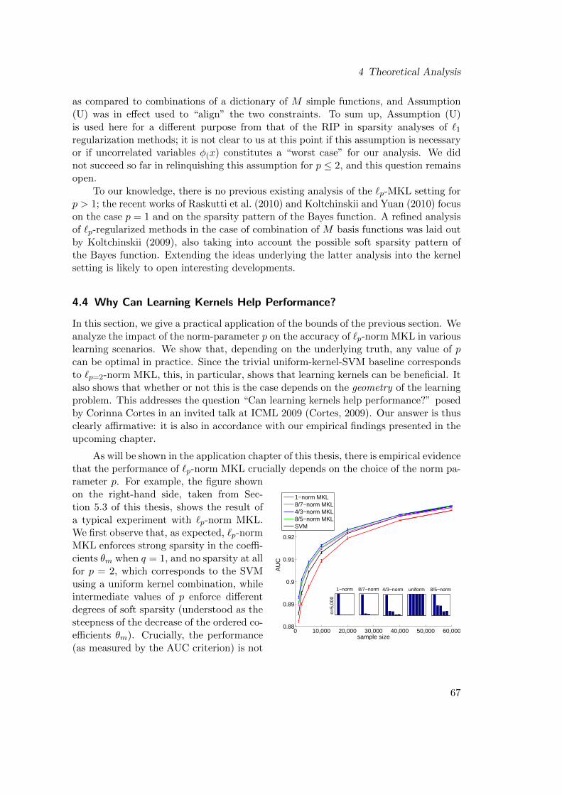
4 Theoretical Analysis
as compared to combinations of a dictionary of M simple functions, and Assumption(U) was in effect used to “align” the two constraints. To sum up, Assumption (U)is used here for a different purpose from that of the RIP in sparsity analyses of `1regularization methods; it is not clear to us at this point if this assumption is necessaryor if uncorrelated variables φ(x) constitutes a “worst case” for our analysis. We didnot succeed so far in relinquishing this assumption for p ≤ 2, and this question remainsopen.
To our knowledge, there is no previous existing analysis of the `p-MKL setting forp > 1; the recent works of Raskutti et al. (2010) and Koltchinskii and Yuan (2010) focuson the case p = 1 and on the sparsity pattern of the Bayes function. A refined analysisof `p-regularized methods in the case of combination of M basis functions was laid outby Koltchinskii (2009), also taking into account the possible soft sparsity pattern ofthe Bayes function. Extending the ideas underlying the latter analysis into the kernelsetting is likely to open interesting developments.
4.4 Why Can Learning Kernels Help Performance?
In this section, we give a practical application of the bounds of the previous section. Weanalyze the impact of the norm-parameter p on the accuracy of `p-norm MKL in variouslearning scenarios. We show that, depending on the underlying truth, any value of pcan be optimal in practice. Since the trivial uniform-kernel-SVM baseline correspondsto `p=2-norm MKL, this, in particular, shows that learning kernels can be beneficial. Italso shows that whether or not this is the case depends on the geometry of the learningproblem. This addresses the question “Can learning kernels help performance?” posedby Corinna Cortes in an invited talk at ICML 2009 (Cortes, 2009). Our answer is thusclearly affirmative: it is also in accordance with our empirical findings presented in theupcoming chapter.
As will be shown in the application chapter of this thesis, there is empirical evidencethat the performance of `p-norm MKL crucially depends on the choice of the norm pa-
0 10,000 20,000 30,000 40,000 50,000 60,0000.88
0.89
0.9
0.91
0.92
0.93
sample size
AU
C
1−norm MKL8/7−norm MKL4/3−norm MKL8/5−norm MKLSVM
8/5−normuniform4/3−norm8/7−norm1−norm
n=5,
000
rameter p. For example, the figure shownon the right-hand side, taken from Sec-tion 5.3 of this thesis, shows the result ofa typical experiment with `p-norm MKL.We first observe that, as expected, `p-normMKL enforces strong sparsity in the coeffi-cients θm when q = 1, and no sparsity at allfor p = 2, which corresponds to the SVMusing a uniform kernel combination, whileintermediate values of p enforce differentdegrees of soft sparsity (understood as thesteepness of the decrease of the ordered co-efficients θm). Crucially, the performance(as measured by the AUC criterion) is not
67
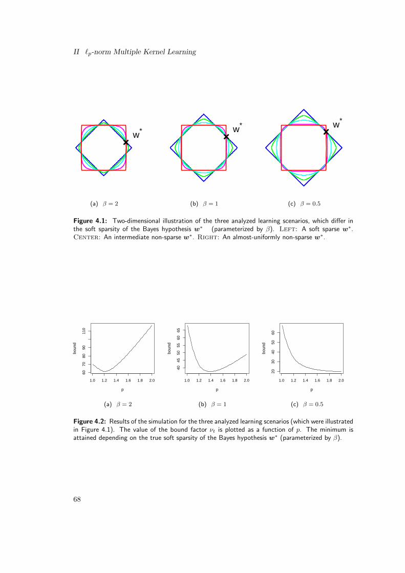
II `p-norm Multiple Kernel Learning
w*
(a) β = 2
w*
(b) β = 1
w*
(c) β = 0.5
Figure 4.1: Two-dimensional illustration of the three analyzed learning scenarios, which differ inthe soft sparsity of the Bayes hypothesis w∗ (parameterized by β). Left: A soft sparse w∗.Center: An intermediate non-sparse w∗. Right: An almost-uniformly non-sparse w∗.
1.0 1.2 1.4 1.6 1.8 2.0
6070
8090
110
p
boun
d
(a) β = 2
1.0 1.2 1.4 1.6 1.8 2.0
4045
5055
6065
p
boun
d
(b) β = 1
1.0 1.2 1.4 1.6 1.8 2.0
2030
4050
60
p
boun
d
(c) β = 0.5
Figure 4.2: Results of the simulation for the three analyzed learning scenarios (which were illustratedin Figure 4.1). The value of the bound factor νt is plotted as a function of p. The minimum isattained depending on the true soft sparsity of the Bayes hypothesis w∗ (parameterized by β).
68
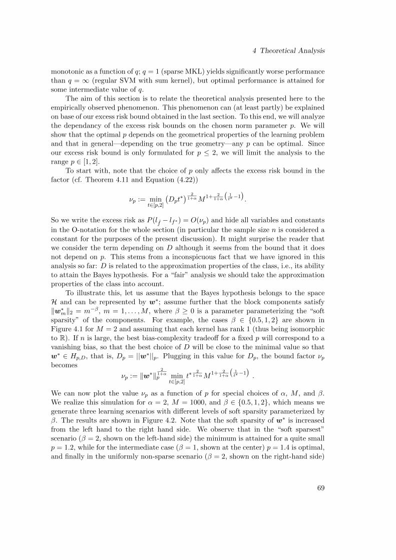
4 Theoretical Analysis
monotonic as a function of q; q = 1 (sparse MKL) yields significantly worse performancethan q = ∞ (regular SVM with sum kernel), but optimal performance is attained forsome intermediate value of q.
The aim of this section is to relate the theoretical analysis presented here to theempirically observed phenomenon. This phenomenon can (at least partly) be explainedon base of our excess risk bound obtained in the last section. To this end, we will analyzethe dependancy of the excess risk bounds on the chosen norm parameter p. We willshow that the optimal p depends on the geometrical properties of the learning problemand that in general—depending on the true geometry—any p can be optimal. Sinceour excess risk bound is only formulated for p ≤ 2, we will limit the analysis to therange p ∈ [1, 2].
To start with, note that the choice of p only affects the excess risk bound in thefactor (cf. Theorem 4.11 and Equation (4.22))
νp := mint∈[p,2]
(Dpt
∗) 21+αM1+ 2
1+α
(1t∗−1
).
So we write the excess risk as P (lf − lf∗) = O(νp) and hide all variables and constants
in the O-notation for the whole section (in particular the sample size n is considered aconstant for the purposes of the present discussion). It might surprise the reader thatwe consider the term depending on D although it seems from the bound that it doesnot depend on p. This stems from a inconspicuous fact that we have ignored in thisanalysis so far: D is related to the approximation properties of the class, i.e., its abilityto attain the Bayes hypothesis. For a “fair” analysis we should take the approximationproperties of the class into account.
To illustrate this, let us assume that the Bayes hypothesis belongs to the spaceH and can be represented by w∗; assume further that the block components satisfy‖w∗m‖2 = m−β, m = 1, . . . ,M , where β ≥ 0 is a parameter parameterizing the “softsparsity” of the components. For example, the cases β ∈ 0.5, 1, 2 are shown inFigure 4.1 for M = 2 and assuming that each kernel has rank 1 (thus being isomorphicto R). If n is large, the best bias-complexity tradeoff for a fixed p will correspond to avanishing bias, so that the best choice of D will be close to the minimal value so thatw∗ ∈ Hp,D, that is, Dp = ||w∗||p. Plugging in this value for Dp, the bound factor νpbecomes
νp := ‖w∗‖2
1+αp min
t∈[p,2]t∗
21+αM1+ 2
1+α
(1t∗−1
).
We can now plot the value νp as a function of p for special choices of α, M , and β.We realize this simulation for α = 2, M = 1000, and β ∈ 0.5, 1, 2, which means wegenerate three learning scenarios with different levels of soft sparsity parameterized byβ. The results are shown in Figure 4.2. Note that the soft sparsity of w∗ is increasedfrom the left hand to the right hand side. We observe that in the “soft sparsest”scenario (β = 2, shown on the left-hand side) the minimum is attained for a quite smallp = 1.2, while for the intermediate case (β = 1, shown at the center) p = 1.4 is optimal,and finally in the uniformly non-sparse scenario (β = 2, shown on the right-hand side)
69
II `p-norm Multiple Kernel Learning
the choice of p = 2 is optimal (although even a higher p could be optimal, but ourbound is only valid for p ∈ [1, 2]).
This means that if the true Bayes hypothesis has an intermediately dense repre-sentation, our bound gives the strongest generalization guarantees to `p-norm MKLusing an intermediate choice of p. This is also intuitive: if the truth exhibits some softsparsity but is not strongly sparse, we expect non-sparse MKL to perform better thanstrongly sparse MKL or the unweighted-sum kernel SVM.
4.5 Summary and Discussion
We justified the proposed `p-norm multiple kernel learning methodology from a the-oretical point of view. Our analysis is built upon the established framework of localRademacher complexities (Koltchinskii and Panchenko, 2002; Koltchinskii, 2006): wederived tight upper bounds on the local Rademacher complexity of the hypothesis classassociated with `p-norm MKL, yielding excess risk bounds with fast convergence rates
of the order O(n−α
1+α ), where α is the minimum eigenvalue decay rate of the individ-ual kernels, thus being tighter than existing bounds for `p>1-norm MKL, which only
achieved slow convergence rates of the order O(n−12 ). We also showed a lower bound
on the local complexity, which, up to constants, matches the upper bounds, showingthat our results are tight. For the upper bounds to hold, we used an assumption on theuncorrelatedness of the kernels; a similar assumption was also recently used by Raskuttiet al. (2010), but in the different context of sparse recovery. We also remark that itwould be interesting to even refine the analysis beyond local Rademacher complexities;Bartlett and Mendelson (2006) would be a good starting point for such an undertaking.
Beside reporting on the worst-case bounds, we also connected the minimal valuesof the bounds with the geometry of the underlying learning scenario (namely, thesoft sparsity of the Bayes hypothesis), in particular, demonstrating that for a largerange of learning scenarios `p-norm MKL attains a strictly “better” (i.e., lower) boundthan classical `1-norm MKL and the SVM using a uniform kernel combination. Thistheoretically justifies using `p-norm MKL and multiple kernel learning in general. Thisis notable since even the tightest previous analyses such as the one carried out by Corteset al. (2010a) were not able to answer the research question “Can learning kernels helpperformance?” (Cortes, 2009).
70
5 Empirical Analysis and Applications
5 Empirical Analysis and Applications
In this chapter, we present an empirical analysis of `p-norm MKL. We first exemplifyour experimental methodology on artificial data and real-world data, shedding lighton the appropriateness of a high/low p in several learning scenarios that differ in thesparseness of the underlying Bayes hypothesis. We then apply the proposed `p-normMKL on diverse, highly topical real-world problems from the domains of bioinformaticsand computer vision that traditionally come with various heterogeneous feature groups/ kernels and thus are very attractive for multiple kernel learning.
The main contributions in this chapter are the following:
• We investigate why learning kernels can help performance on artificial data, where wefind the bounds well predicting the optimal value of the parameter p.
• We show that `p-norm MKL achieves accuracies in highly topical and central real-world applications from the domains of bioinformatics and computer vision that gobeyond the state-of-the-art:
(a) we apply `p-norm MKL to protein fold prediction, experimenting on the recentlyreleased dingshen data, yielding an accuracy improvement of 6%
(b) we apply `p-norm MKL to DNA transcription start site (TSS) prediction, train-ing our large-scale implementation on 60,000 training examples and outperform-ing the uniform-sum kernel SVM (which recently was confirmed to be leading ina comparison of 19 DNA TSS predictors)
(c) we apply `p-norm MKL to visual image classification, a computer vision applica-tion, significantly increasing the predictive accuracy for all concept classes andby 1.5 AP point in average.
• We introduce a methodology based on kernel alignments and the theoretical boundsto investigate/estimate our findings, i.e., the optimality of a particular p.
Parts of this chapter are based on:
M. Kloft, U. Brefeld, S. Sonnenburg, P. Laskov, K.-R. Muller, and A. Zien. Efficientand accurate lp-norm multiple kernel learning. In NIPS 2009, pages 997–1005. MITPress, 2009.
M. Kloft, U. Brefeld, S. Sonnenburg, and A. Zien. Lp-norm multiple kernel learning.Journal of Machine Learning Research (JMLR), 12:953–997, 2011.
A. Binder, S. Nakajima, M. Kloft, C. Muller, W. Wojcikiewicz, U. Brefeld, K.-R.Muller, and M. Kawanabe. Multiple kernel learning for object classification. Submit-ted to IEEE TPAMI. A preliminary version is published in IBIS 2010.
5.1 Goal and Experimental Methodology
Goal The goal of the application chapter of this thesis is to confirm the followinghypotheses:
1. In practical applications that are characterized by multiple heterogeneous kernels/ feature mappings, `p-norm MKL often yields more accurate prediction models
71
II `p-norm Multiple Kernel Learning
than `1-norm MKL, the SVM using a uniform kernel combination, and the single-kernel SVM with the kernel tuned by model selection.
2. For medium and large training set sizes n, the bounds presented in the previ-ous chapter reflect the empirically best-performing parameter p (rendering themattractive for model selection) while for small n the Bayes hypothesis might beinsufficiently approximated, leading to an overestimation of the optimal p.
5.1.1 Methodology
To investigate the validity of the above hypotheses, we experiment on cutting-edgedata sets taken from diverse application domains. Thereby, we deploy the followingexperimental protocol:
1. Application description and goal First, the application’s problem settingis described and the goal is defined; usually this is maximizing the predictionaccuracy or an application-specific standard performance measure such as MCC,AUC, or AP (see below for definitions of this measures).
2. Experimental setup Second, we report on the employed data set and theexperimental setup. Usually, we deploy random sampling of disjoint training,validation, and test sets, where the number of repetitions is chosen such that thestandard errors indicate significance of the results (usually 100–250 repetitions).We always compare our results to the ones achieved by `1-norm MKL and theSVM using a uniform kernel combination. Often, the single-kernel-SVM perfor-mance is known from the literature, where it was either compared to `1-normMKL or the SVM using an uniform kernel combination; in all of our experiments,the latter two baselines are contained in the set of models, thus allowing to alsocompare `p-norm MKL to the single-kernel SVM without actually recomputingit. However, if the single-kernel performance is not known from the literature, wecompute this baseline. We compare various `p-norm MKL variants and deploy alocal search for the optimal p. In all experiments, we optimize the relative dualitygap up to a precision of 0.001.
3. Results The results of the experiment are shown in terms of an application-specific standard performance measure along with corresponding standard errors.In one case we use a benchmark data set that comes with a single test set; here,we compute the standard deviation by repeatedly and randomly splitting the testset in two parts of equal size.
4. Interpretation The kernel weights θ as output by MKL are shown. Thisindicates which kernels contribute most to the final MKL solution. We also reporton the alignments of the given kernel matrices with respect to the Frobenius scalarproduct. This can be of help in identifying redundant and complementary kernels.
72
5 Empirical Analysis and Applications
5. Bound We compute the factor of the theoretical bound that depends on thenorm parameter p, thus being relevant for the estimation of the appropriateness ofa small/large p. We focus on global Rademacher complexity as it does not involvethe additional parameter α that is unknown in practice, which corresponds totaking α ≈ 1 in the local complexity (this can be seen as a conservative choice:the (empirical) global bound can directly be evaluated from the kernel matricesat hand without knowledge of the true spectra of the kernels). As discussed inSection 4.4, we require the Bayes hypothesis to be in the hypothesis set so that therelevant bound factor is νglobp = mint≥p
√t∗ ‖wBayes‖2,pM
1/t∗ . Since this requiresknowledge of the Bayes hypothesis wBayes, we take the one hypothesis wmkl
output by MKL that performed best in the experiments (using the empiricallyoptimal p) as an approximation ofwBayes. Note that we expect this approximationgetting tighter with increasing n. For the computation of wmkl, we take mediansover 100 runs; for the multi-class data sets the medians are also computed overthe classes.
6. Summary and discussion Each experiment is concluded by a short discussion.
5.1.2 Evaluation measures
To assess the effectiveness of the compared methods, we use the following evaluationmeasures. Let (xt, yt)t∈T be a set of example/label test pairs and f : X → Y ahypothesis function; let Y = −1, 1.
• The test error is defined as TE =∑
t∈T 1f(xt)6=yt , where 1 denotes the indicatorfunction.
• The area under the receiver operating characteristic curve (AUC) is defined asthe integral of the receiver operating characteristic (ROC) curve. Thereby, theROC curve is the true positive rate (fraction of correctly positively classified datapoints) as a function of the false positive rate (fraction of incorrectly positivelyclassified data points). For (multi-) kernel methods and linear methods the vari-ous values of the false positive rate correspond to translating the bias b. The AUCranges in the interval [0, 1], where 0.5 is attained by a completely random clas-sifier (random label assignment); thus, reasonable classifiers should attain valueshigher than 0.5.
• The Matthews correlation coefficient (MCC) or φ coefficient is defined as
MCC =TP× TN− FP× FN√
(TP + FP)(TP + FN)(TN + FP)(TN + FN),
where FP and TP are the number of correctly and incorrectly positively classifieddata points, respectively, and FN and TN are defined analogously for negativelyclassified data points. The MCC ranges in the interval [−1, 1] where MCC = 0corresponds to a random prediction.
73
II `p-norm Multiple Kernel Learning
• Average precision: let t1, . . . , tn be the indexes corresponding to sorting the clas-sifier outputs f(xt) in decreasing order. Denote the number of positive andnegative examples by n+ and n−, respectively; define the precision at k bypk = 1
k
∑ki=1 1yti=1 (the number of correctly positively classified examples among
the top-k ranked ones). Then, the average precision is defined as
AP =1
n+
n∑k=1
pk1ytk=1
(thus it is the precision at k averaged over all k). The AP ranges in the interval[0, 1] and somewhat depends on the skewness of the classes: a random classifierattains AP = n+
n++n−.
Probably the most standard measure in machine learning is the test error. However, inapplications with unbalanced class sizes it is recommended to use one of the alternativemeasures, that is, MCC, AUC, or AP. Traditionally, some applications come withcertain standard evaluation measures. For example, in image categorization, as aninformation retrieval application, AP is the standard measure and, in bioinformatics,MCC and AUC are frequently used.
Kernel aligments As a tool for the explorative analysis of the obtained results, we alsoemploy the kernel alignment introduced by Cristianini et al. (2002), which measuresthe similarity of two matrices and can be interpreted as a (hyper-) kernel acting onthe space of kernel functions (Ong et al., 2005). Let K and K be two kernel matricescorresponding to kernels k and k, respectively; then, the alignment of K and K isdefined as the cosine of the angle between K and K:
A(K, K) :=〈K, K〉F‖K‖F ‖K‖F
, (5.1)
where 〈K, K〉F :=∑n
i,j=1 k(xi, xj)k(xi, xj) denotes the Frobenius scalar product and
‖K‖F :=√〈K,K〉F the corresponding norm.
In many applications, centering of the kernels is recommended before comput-ing the alignment (Cortes et al., 2010b); for example, SVMs and many other kernel-based learning algorithms are invariant against mean shifts in the corresponding Hilbertspaces. Centering K in the corresponding feature space can easily be achieved by com-puting the product HKH, where H := I − 1
n11> with I being the identity matrix ofsize n and 1 a column vector of all ones.
5.2 Case Study 1: Toy Experiment
We now present a toy experiment that serves the following purposes:
• empirically confirming some of our claims in a controlled environment, that is,one where we know the underlying distribution generating the data
74
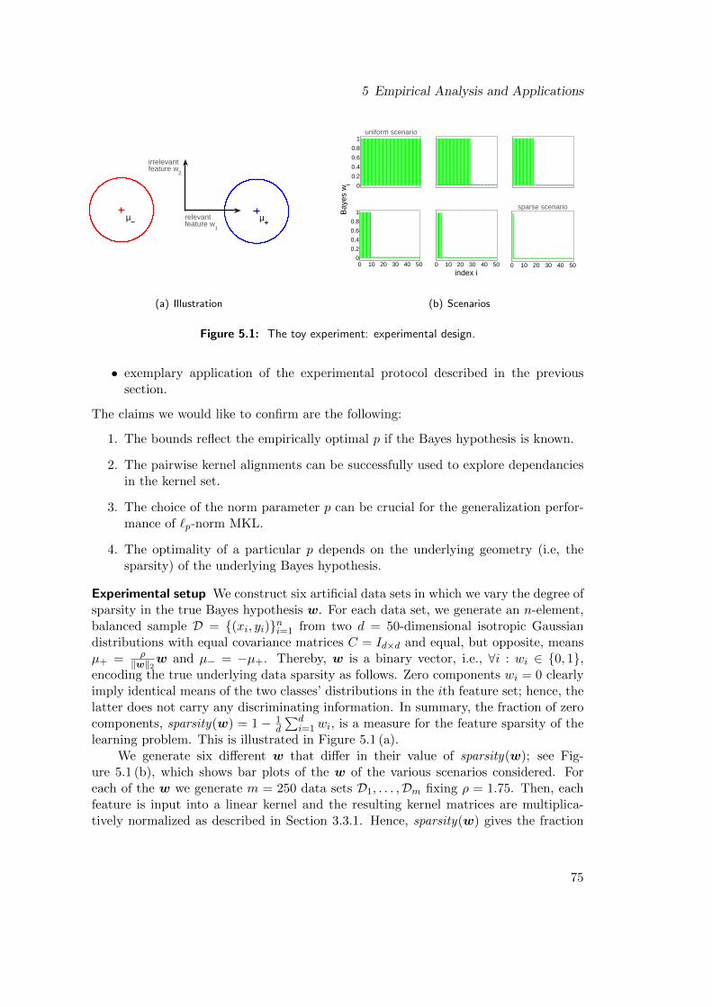
5 Empirical Analysis and Applications
irrelevantfeature w
2
relevantfeature w
1
µ+
µ−
(a) Illustration
0
0.2
0.4
0.6
0.8
1uniform scenario
0 10 20 30 40 500
0.2
0.4
0.6
0.8
1Bay
es w
i
0 10 20 30 40 50
index i0 10 20 30 40 50
sparse scenario
(b) Scenarios
Figure 5.1: The toy experiment: experimental design.
• exemplary application of the experimental protocol described in the previoussection.
The claims we would like to confirm are the following:
1. The bounds reflect the empirically optimal p if the Bayes hypothesis is known.
2. The pairwise kernel alignments can be successfully used to explore dependanciesin the kernel set.
3. The choice of the norm parameter p can be crucial for the generalization perfor-mance of `p-norm MKL.
4. The optimality of a particular p depends on the underlying geometry (i.e, thesparsity) of the underlying Bayes hypothesis.
Experimental setup We construct six artificial data sets in which we vary the degree ofsparsity in the true Bayes hypothesis w. For each data set, we generate an n-element,balanced sample D = (xi, yi)ni=1 from two d = 50-dimensional isotropic Gaussiandistributions with equal covariance matrices C = Id×d and equal, but opposite, meansµ+ = ρ
‖w‖2w and µ− = −µ+. Thereby, w is a binary vector, i.e., ∀i : wi ∈ 0, 1,encoding the true underlying data sparsity as follows. Zero components wi = 0 clearlyimply identical means of the two classes’ distributions in the ith feature set; hence, thelatter does not carry any discriminating information. In summary, the fraction of zerocomponents, sparsity(w) = 1− 1
d
∑di=1wi, is a measure for the feature sparsity of the
learning problem. This is illustrated in Figure 5.1 (a).We generate six different w that differ in their value of sparsity(w); see Fig-
ure 5.1 (b), which shows bar plots of the w of the various scenarios considered. Foreach of the w we generate m = 250 data sets D1, . . . ,Dm fixing ρ = 1.75. Then, eachfeature is input into a linear kernel and the resulting kernel matrices are multiplica-tively normalized as described in Section 3.3.1. Hence, sparsity(w) gives the fraction
75
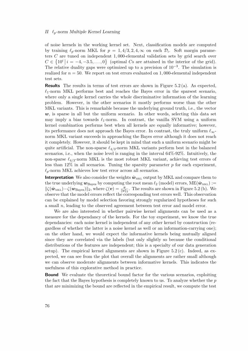
II `p-norm Multiple Kernel Learning
of noise kernels in the working kernel set. Next, classification models are computedby training `p-norm MKL for p = 1, 4/3, 2, 4,∞ on each Di. Soft margin parame-ters C are tuned on independent 1, 000-elemental validation sets by grid search overC ∈
10i∣∣ i = −4,−3.5, . . . , 0
(optimal Cs are attained in the interior of the grid).
The relative duality gaps were optimized up to a precision of 10−3. The simulation isrealized for n = 50. We report on test errors evaluated on 1, 000-elemental independenttest sets.
Results The results in terms of test errors are shown in Figure 5.2 (a). As expected,`1-norm MKL performs best and reaches the Bayes error in the sparsest scenario,where only a single kernel carries the whole discriminative information of the learningproblem. However, in the other scenarios it mostly performs worse than the otherMKL variants. This is remarkable because the underlying ground truth, i.e., the vectorw, is sparse in all but the uniform scenario. In other words, selecting this data setmay imply a bias towards `1-norm. In contrast, the vanilla SVM using a uniformkernel combination performs best when all kernels are equally informative; however,its performance does not approach the Bayes error. In contrast, the truly uniform `∞-norm MKL variant succeeds in approaching the Bayes error although it does not reachit completely. However, it should be kept in mind that such a uniform scenario might bequite artificial. The non-sparse `4/3-norm MKL variants perform best in the balancedscenarios, i.e., when the noise level is ranging in the interval 64%-92%. Intuitively, thenon-sparse `4/3-norm MKL is the most robust MKL variant, achieving test errors ofless than 12% in all scenarios. Tuning the sparsity parameter p for each experiment,`p-norm MKL achieves low test error across all scenarios.
Interpretation We also consider the weights wmkl output by MKL and compare them tothe true underlyingwBayes by computing the root mean `2 (model) errors, ME(wmkl) :=‖ζ(wmkl)−ζ(wBayes)‖2, where ζ(v) = v
‖v‖2 . The results are shown in Figure 5.2 (b). Weobserve that the model errors reflect the corresponding test errors well. This observationcan be explained by model selection favoring strongly regularized hypotheses for sucha small n, leading to the observed agreement between test error and model error.
We are also interested in whether pairwise kernel alignments can be used as ameasure for the dependancy of the kernels. For the toy experiment, we know the truedependancies: each noise kernel is independent of any other kernel by construction (re-gardless of whether the latter is a noise kernel as well or an information-carrying one);on the other hand, we would expect the informative kernels being mutually alignedsince they are correlated via the labels (but only slightly so because the conditionaldistributions of the features are independent; this is a specialty of our data generationsetup). The empirical kernel alignments are shown in Figure 5.2 (c). Indeed, as ex-pected, we can see from the plot that overall the alignments are rather small althoughwe can observe moderate alignments between informative kernels. This indicates theusefulness of this explorative method in practice.
Bound We evaluate the theoretical bound factor for the various scenarios, exploitingthe fact that the Bayes hypothesis is completely known to us. To analyze whether the pthat are minimizing the bound are reflected in the empirical result, we compute the test
76
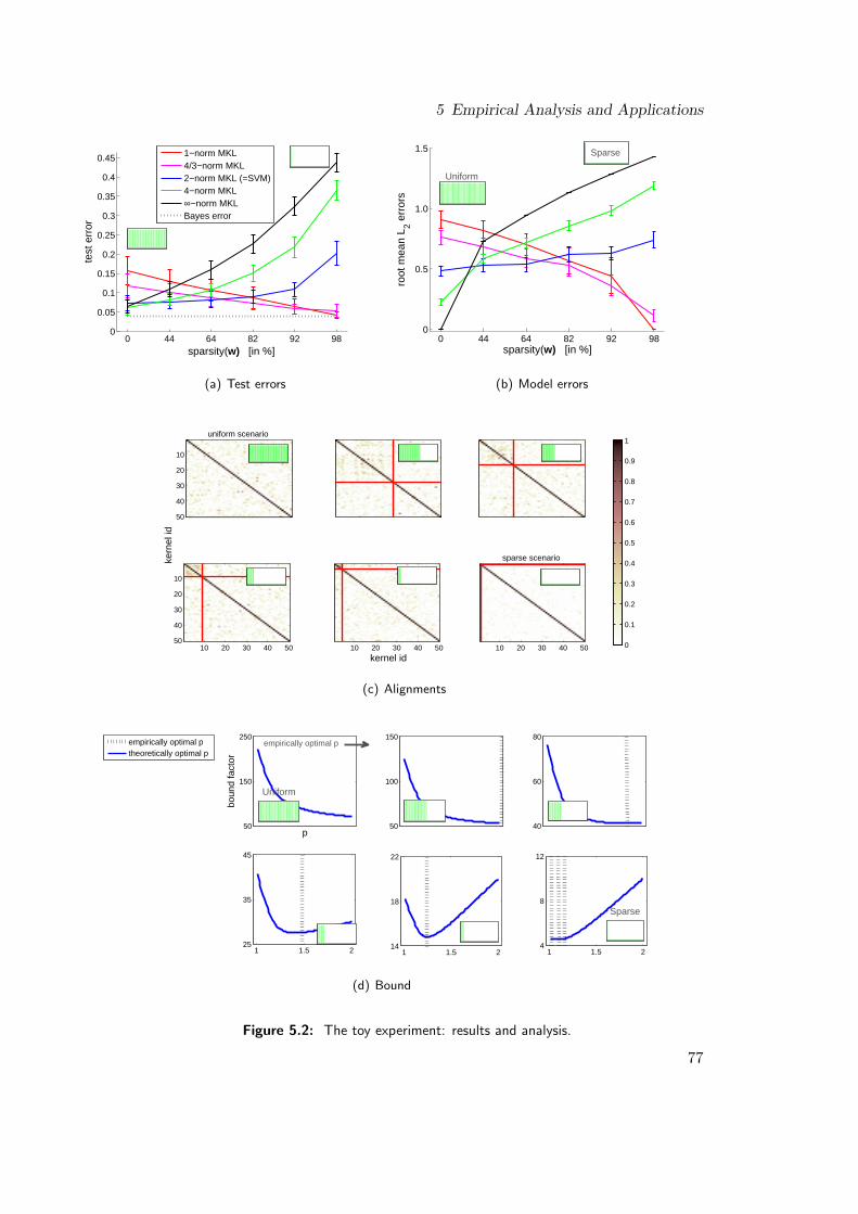
5 Empirical Analysis and Applications
0 44 64 82 92 980
0.05
0.1
0.15
0.2
0.25
0.3
0.35
0.4
0.45
sparsity(w) [in %]
test
err
or
Uniform
1−norm MKL4/3−norm MKL2−norm MKL (=SVM)4−norm MKL∞−norm MKLBayes error
(a) Test errors
0 44 64 82 92 980
0.5
1.0
1.5
sparsity(w) [in %]
root
mea
n L 2 e
rror
s
Uniform
Sparse
Uniform
(b) Model errors
uniform scenario
10
20
30
40
50
10 20 30 40 50
10
20
30
40
50
10 20 30 40 50
sparse scenario
10 20 30 40 50 0
0.1
0.2
0.3
0.4
0.5
0.6
0.7
0.8
0.9
1
kern
el id
kernel id
(c) Alignments
50
150
250
p
boun
d fa
ctor
50
100
150
40
60
80
1 1.5 225
35
45
1 1.5 214
18
22
1 1.5 24
8
12
Uniform
Sparse
empirically optimal ptheoretically optimal p
empirically optimal p
(d) Bound
Figure 5.2: The toy experiment: results and analysis.
77
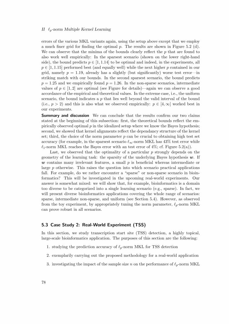
II `p-norm Multiple Kernel Learning
errors of the various MKL variants again, using the setup above except that we employa much finer grid for finding the optimal p. The results are shown in Figure 5.2 (d).We can observe that the minima of the bounds clearly reflect the p that are found toalso work well empirically: In the sparsest scenario (shown on the lower right-handside), the bound predicts p ∈ [1, 1.14] to be optimal and indeed, in the experiments, allp ∈ [1, 1.15] performed best (and equally well) while the next higher p contained in ourgrid, namely p = 1.19, already has a slightly (but significantly) worse test error—instriking match with our bounds. In the second sparsest scenario, the bound predictsp = 1.25 and we empirically found p = 1.26. In the non-sparse scenarios, intermediatevalues of p ∈ [1, 2] are optimal (see Figure for details)—again we can observe a goodaccordance of the empirical and theoretical values. In the extreme case, i.e., the uniformscenario, the bound indicates a p that lies well beyond the valid interval of the bound(i.e., p > 2) and this is also what we observed empirically: p ∈ [4,∞] worked best inour experiments.
Summary and discussion We can conclude that the results confirm our two claimsstated at the beginning of this subsection: first, the theoretical bounds reflect the em-pirically observed optimal p in the idealized setup where we know the Bayes hypothesis;second, we showed that kernel alignments reflect the dependancy structure of the kernelset; third, the choice of the norm parameter p can be crucial to obtaining high test setaccuracy (for example, in the sparsest scenario `∞-norm MKL has 43% test error while`1-norm MKL reaches the Bayes error with an test error of 4%; cf. Figure 5.2(a)).
Last, we observed that the optimality of a particular p strongly depends on thegeometry of the learning task: the sparsity of the underlying Bayes hypothesis w. Ifw contains many irrelevant features, a small p is beneficial whereas intermediate orlarge p otherwise. This raises the question into which scenario practical applicationsfall. For example, do we rather encounter a “sparse” or non-sparse scenario in bioin-formatics? This will be investigated in the upcoming real-world experiments. Ouranswer is somewhat mixed: we will show that, for example, bioinformatics is a domaintoo diverse to be categorized into a single learning scenario (e.g., sparse). In fact, wewill present diverse bioinformatics applications covering the whole range of scenarios:sparse, intermediate non-sparse, and uniform (see Section 5.4). However, as observedfrom the toy experiment, by appropriately tuning the norm parameter, `p-norm MKLcan prove robust in all scenarios.
5.3 Case Study 2: Real-World Experiment (TSS)
In this section, we study transcription start site (TSS) detection, a highly topical,large-scale bioinformatics application. The purposes of this section are the following:
1. studying the prediction accuracy of `p-norm MKL for TSS detection
2. exemplarily carrying out the proposed methodology for a real-world application
3. investigating the impact of the sample size n on the performance of `p-norm MKL
78
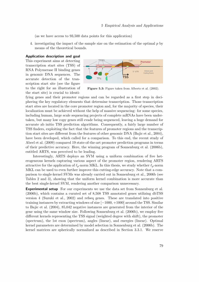
5 Empirical Analysis and Applications
(as we have access to 93,500 data points for this application)
4. investigating the impact of the sample size on the estimation of the optimal p bymeans of the theoretical bounds.
Figure 5.3: Figure taken from Alberts et al. (2002).
Application description and goalThis experiment aims at detectingtranscription start sites (TSS) ofRNA Polymerase II binding genesin genomic DNA sequences. Theaccurate detection of the tran-scription start site (see the figureto the right for an illustration ofthe start site) is crucial to identi-fying genes and their promoter regions and can be regarded as a first step in deci-phering the key regulatory elements that determine transcription. Those transcriptionstart sites are located in the core promoter region and, for the majority of species, theirlocalization must be achieved without the help of massive sequencing: for some species,including human, large scale sequencing projects of complete mRNAs have been under-taken, but many low copy genes still evade being sequenced, leaving a huge demand foraccurate ab initio TSS prediction algorithms. Consequently, a fairly large number ofTSS finders, exploiting the fact that the features of promoter regions and the transcrip-tion start sites are different from the features of other genomic DNA (Bajic et al., 2004),have been developed, which called for a comparison. To this end, the recent study ofAbeel et al. (2009) compared 19 state-of-the-art promoter prediction programs in termsof their predictive accuracy. Here, the winning program of Sonnenburg et al. (2006b),entitled ARTS, was perceived to be leading.
Interestingly, ARTS deploys an SVM using a uniform combination of five het-erogeneous kernels capturing various aspect of the promoter region, rendering ARTSattractive for the application of `p-norm MKL. In this thesis, we study whether `p-normMKL can be used to even further improve this cutting-edge accuracy. Note that a com-parison to single-kernel SVMs was already carried out in Sonnenburg et al., 2006b (seeTables 2 and 3), showing that the uniform kernel combination is more accurate thanthe best single-kernel SVM, rendering another comparison unnecessary.
Experimental setup For our experiments we use the data set from Sonnenburg et al.(2006b), which contains a curated set of 8,508 TSS annotated genes utilizing dbTSSversion 4 (Suzuki et al., 2002) and refseq genes. These are translated into positivetraining instances by extracting windows of size [−1000,+1000] around the TSS. Similarto Bajic et al. (2004), 85,042 negative instances are generated from the interior of thegene using the same window size. Following Sonnenburg et al. (2006b), we employ fivedifferent kernels representing the TSS signal (weighted degree with shift), the promoter(spectrum), the 1st exon (spectrum), angles (linear), and energies (linear). Optimalkernel parameters are determined by model selection in Sonnenburg et al. (2006b). Thekernel matrices are spherically normalized as described in Section 3.3.1. We reserve
79
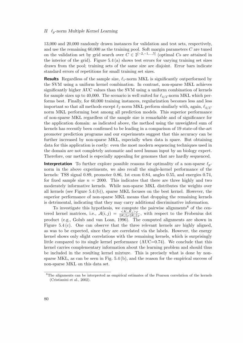
II `p-norm Multiple Kernel Learning
13,000 and 20,000 randomly drawn instances for validation and test sets, respectively,and use the remaining 60,000 as the training pool. Soft margin parameters C are tunedon the validation set by grid search over C ∈ 2[−2,−1,...,5] (optimal Cs are attained inthe interior of the grid). Figure 5.4 (a) shows test errors for varying training set sizesdrawn from the pool; training sets of the same size are disjoint. Error bars indicatestandard errors of repetitions for small training set sizes.
Results Regardless of the sample size, `1-norm MKL is significantly outperformed bythe SVM using a uniform kernel combination. In contrast, non-sparse MKL achievessignificantly higher AUC values than the SVM using a uniform combination of kernelsfor sample sizes up to 40,000. The scenario is well suited for `4/3-norm MKL which per-forms best. Finally, for 60,000 training instances, regularization becomes less and lessimportant so that all methods except `1-norm MKL perform similarly with, again, `4/3-norm MKL performing best among all prediction models. This superior performanceof non-sparse MKL regardless of the sample size is remarkable and of significance forthe application domain: as indicated above, the method using the unweighted sum ofkernels has recently been confirmed to be leading in a comparison of 19 state-of-the-artpromoter prediction programs and our experiments suggest that this accuracy can befurther increased by non-sparse MKL, especially when data is spare. But obtainingdata for this application is costly: even the most modern sequencing techniques used inthe domain are not completely automatic and need human input by an biology expert.Therefore, our method is especially appealing for genomes that are hardly sequenced.
Interpretation To further explore possible reasons for optimality of a non-sparse `p-norm in the above experiments, we also recall the single-kernel performance of thekernels: TSS signal 0.89, promoter 0.86, 1st exon 0.84, angles 0.55, and energies 0.74,for fixed sample size n = 2000. This indicates that there are three highly and twomoderately informative kernels. While non-sparse MKL distributes the weights overall kernels (see Figure 5.4 (b)), sparse MKL focuses on the best kernel. However, thesuperior performance of non-sparse MKL means that dropping the remaining kernelsis detrimental, indicating that they may carry additional discriminative information.
To investigate this hypothesis, we compute the pairwise alignments8 of the cen-tered kernel matrices, i.e., A(i, j) =
<Ki,Kj>F‖Ki‖F ‖Kj‖F , with respect to the Frobenius dot
product (e.g., Golub and van Loan, 1996). The computed alignments are shown inFigure 5.4 (c). One can observe that the three relevant kernels are highly aligned,as was to be expected, since they are correlated via the labels. However, the energykernel shows only slight correlations with the remaining kernels, which is surprisinglylittle compared to its single kernel performance (AUC=0.74). We conclude that thiskernel carries complementary information about the learning problem and should thusbe included in the resulting kernel mixture. This is precisely what is done by non-sparse MKL, as can be seen in Fig. 5.4 (b), and the reason for the empirical success ofnon-sparse MKL on this data set.
8The alignments can be interpreted as empirical estimates of the Pearson correlation of the kernels(Cristianini et al., 2002).
80
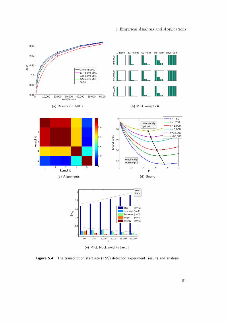
5 Empirical Analysis and Applications
0 10,000 20,000 30,000 40,000 50,000 60,0000.88
0.89
0.9
0.91
0.92
0.93
sample size
AU
C
1−norm MKL8/7−norm MKL4/3−norm MKL8/5−norm MKLSVM
(a) Results (in AUC)
1−norm
n=5,
000
8/7−norm 4/3−norm 8/5−norm unw.−sum
n=20
,000
n=60
,000
(b) MKL weights θ
(c) Alignments
1 1.2 1.4 1.6 1.8 2
2.2
2.4
2.6
2.8
3
p
boun
d fa
ctor
empiricallyoptimal p
n= 50n= 250n= 1,000n= 5,000n=15,000n=60,000
theoreticallyoptimal p
(d) Bound
50 250 1,000 5,000 15,000 60,000
0
0.2
0.4
0.6
0.8
1
n
||wm
||
TSS (m=1)promoter (m=2)1st exon (m=3)angle (m=4)energy (m=5)
trendlines
(e) MKL block weights ‖wm‖
Figure 5.4: The transcription start site (TSS) detection experiment: results and analysis.
81
II `p-norm Multiple Kernel Learning
Bounds For various training set sizes n, we compute the bound factor as a function of p.The results are shown in Figure 5.4 (d). We can observe the optimal p, as predicted bythe theoretical bounds, apparently converging towards the empirically optimal p (whichis p = 4/3) when increasing the training set size n. This results from the approximationof the Bayes hypothesis being tighter for large n: we compute wmkl as output by MKLfor various n (shown in Figure 5.4 (e)) and observe that, with increasing n, MKL tendsto discard the angle and energy kernels; the latter two kernels are of finite rank. Theirlimited complexity renders them less effective for large n. We thus conjecture that theBayes hypothesis is likely to focus on the first three kernels (with an emphasis on theTSS kernel, which also empirically performs best). In this sense, it is not surprisingthat the bound “overestimates” the optimal p: since wmkl is “too uniform” comparedto the Bayes-w, the bound (which has wmkl as an input) leads to overly high estimatesof the optimal p. However, it is interesting that already for n = 60, 000 the bound givesa good estimate (p = 1.48) of the empirically optimal p = 1.33.
Summary and discussion Exemplarily, we carried out the proposed experimentalmethodology for transcription start site detection, a cutting-edge bioinformatics ap-plication. The data set we experimented on was also used in the previous study ofSonnenburg et al. (2006a) and comprises 93,500 instances. We showed that regardlessof the sample size, `p-norm MKL can improve the prediction accuracy over `1-normMKL and the SVM using a uniform kernel combination (which itself outperforms thesingle-kernel SVM using the kernel determined by model selection). This is remarkableand of significance for the application domain: the method using a uniform kernel com-bination was recently confirmed to be the most accurate TSS detector in a comparisonof 19 state-of-the-art models Abeel et al. (2009). Furthermore, we observed that thechoice of n had no impact on the empirical optimality of a particular p. We also eval-uated the theoretical bounds and found that with increasing n they give a more andmore accurate estimation of the optimal p through an increasingly tight approximationof the Bayes hypothesis.
5.4 Bioinformatics Experiments
In this section, we apply `p-norm MKL to diverse, highly topical applications takenfrom the domain of bioinformatics. Many bioinformatics applications are too complexto be described by a single type of feature descriptors; for example, finding transcriptionstart sites in genes can only be done moderately well on the raw sequence information—incorporating complementary information such as binding energies or twistedness ofDNA increases the chance of finding a transcription start site. A challenge is here todeal with the additional noise introduced by those so-called weak features, making itvery appealing for multiple kernel learning.
We recall the toy experiment, which showed that the amount by which `p-normMKL is beneficial in such applications crucially depends on the sparsity/uniformnessof the learning task at hand. We are therefore interested in finding out into which
82
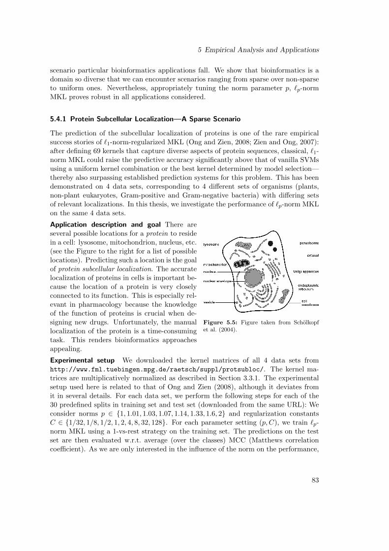
5 Empirical Analysis and Applications
scenario particular bioinformatics applications fall. We show that bioinformatics is adomain so diverse that we can encounter scenarios ranging from sparse over non-sparseto uniform ones. Nevertheless, appropriately tuning the norm parameter p, `p-normMKL proves robust in all applications considered.
5.4.1 Protein Subcellular Localization—A Sparse Scenario
The prediction of the subcellular localization of proteins is one of the rare empiricalsuccess stories of `1-norm-regularized MKL (Ong and Zien, 2008; Zien and Ong, 2007):after defining 69 kernels that capture diverse aspects of protein sequences, classical, `1-norm MKL could raise the predictive accuracy significantly above that of vanilla SVMsusing a uniform kernel combination or the best kernel determined by model selection—thereby also surpassing established prediction systems for this problem. This has beendemonstrated on 4 data sets, corresponding to 4 different sets of organisms (plants,non-plant eukaryotes, Gram-positive and Gram-negative bacteria) with differing setsof relevant localizations. In this thesis, we investigate the performance of `p-norm MKLon the same 4 data sets.
Figure 5.5: Figure taken from Scholkopfet al. (2004).
Application description and goal There areseveral possible locations for a protein to residein a cell: lysosome, mitochondrion, nucleus, etc.(see the Figure to the right for a list of possiblelocations). Predicting such a location is the goalof protein subcellular localization. The accuratelocalization of proteins in cells is important be-cause the location of a protein is very closelyconnected to its function. This is especially rel-evant in pharmacology because the knowledgeof the function of proteins is crucial when de-signing new drugs. Unfortunately, the manuallocalization of the protein is a time-consumingtask. This renders bioinformatics approachesappealing.
Experimental setup We downloaded the kernel matrices of all 4 data sets fromhttp://www.fml.tuebingen.mpg.de/raetsch/suppl/protsubloc/. The kernel ma-trices are multiplicatively normalized as described in Section 3.3.1. The experimentalsetup used here is related to that of Ong and Zien (2008), although it deviates fromit in several details. For each data set, we perform the following steps for each of the30 predefined splits in training set and test set (downloaded from the same URL): Weconsider norms p ∈ 1, 1.01, 1.03, 1.07, 1.14, 1.33, 1.6, 2 and regularization constantsC ∈ 1/32, 1/8, 1/2, 1, 2, 4, 8, 32, 128. For each parameter setting (p, C), we train `p-norm MKL using a 1-vs-rest strategy on the training set. The predictions on the testset are then evaluated w.r.t. average (over the classes) MCC (Matthews correlationcoefficient). As we are only interested in the influence of the norm on the performance,
83
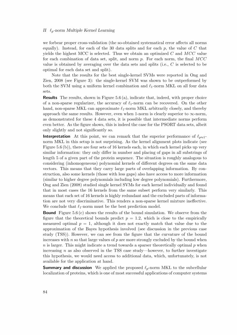
II `p-norm Multiple Kernel Learning
we forbear proper cross-validation (the so-obtained systematical error affects all normsequally). Instead, for each of the 30 data splits and for each p, the value of C thatyields the highest MCC is selected. Thus we obtain an optimized C and MCC valuefor each combination of data set, split, and norm p. For each norm, the final MCCvalue is obtained by averaging over the data sets and splits (i.e., C is selected to beoptimal for each data set and split).
Note that the results for the best single-kernel SVMs were reported in Ong andZien, 2008 (see Figure 3): the single-kernel SVM was shown to be outperformed byboth the SVM using a uniform kernel combination and `1-norm MKL on all four datasets.
Results The results, shown in Figure 5.6 (a), indicate that, indeed, with proper choiceof a non-sparse regularizer, the accuracy of `1-norm can be recovered. On the otherhand, non-sparse MKL can approximate `1-norm MKL arbitrarily closely, and therebyapproach the same results. However, even when 1-norm is clearly superior to ∞-norm,as demonstrated for these 4 data sets, it is possible that intermediate norms performeven better. As the figure shows, this is indeed the case for the PSORT data sets, albeitonly slightly and not significantly so.
Interpretation At this point, we can remark that the superior performance of `p≈1-norm MKL in this setup is not surprising. As the kernel alignment plots indicate (seeFigure 5.6 (b)), there are four sets of 16 kernels each, in which each kernel picks up verysimilar information: they only differ in number and placing of gaps in all substrings oflength 5 of a given part of the protein sequence. The situation is roughly analogous toconsidering (inhomogeneous) polynomial kernels of different degrees on the same datavectors. This means that they carry large parts of overlapping information. By con-struction, also some kernels (those with less gaps) also have access to more information(similar to higher degree polynomials including low degree polynomials). Furthermore,Ong and Zien (2008) studied single kernel SVMs for each kernel individually and foundthat in most cases the 16 kernels from the same subset perform very similarly. Thismeans that each set of 16 kernels is highly redundant and the excluded parts of informa-tion are not very discriminative. This renders a non-sparse kernel mixture ineffective.We conclude that `1-norm must be the best prediction model.
Bound Figure 5.6 (c) shows the results of the bound simulation. We observe from thefigure that the theoretical bounds predict p = 1.2, which is close to the empiricallymeasured optimal p = 1, although it does not exactly match that value due to theapproximation of the Bayes hypothesis involved (see discussion in the previous casestudy (TSS)). However, we can see from the figure that the curvature of the boundincreases with n so that large values of p are more strongly excluded by the bound whenn is larger. This might indicate a trend towards a sparser theoretically optimal p whenincreasing n as also observed in the TSS case study—however, to further investigatethis hypothesis, we would need access to additional data, which, unfortunately, is notavailable for the application at hand.
Summary and discussion We applied the proposed `p-norm MKL to the subcellularlocalization of proteins, which is one of most successful applications of computer systems
84
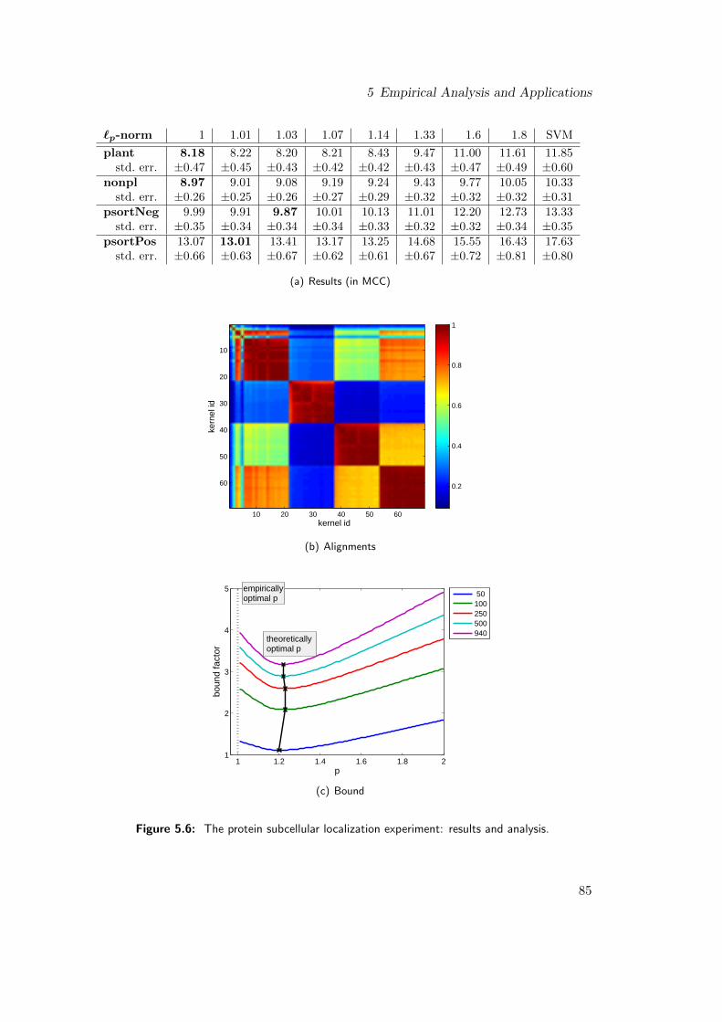
5 Empirical Analysis and Applications
`p-norm 1 1.01 1.03 1.07 1.14 1.33 1.6 1.8 SVM
plant 8.18 8.22 8.20 8.21 8.43 9.47 11.00 11.61 11.85std. err. ±0.47 ±0.45 ±0.43 ±0.42 ±0.42 ±0.43 ±0.47 ±0.49 ±0.60
nonpl 8.97 9.01 9.08 9.19 9.24 9.43 9.77 10.05 10.33std. err. ±0.26 ±0.25 ±0.26 ±0.27 ±0.29 ±0.32 ±0.32 ±0.32 ±0.31
psortNeg 9.99 9.91 9.87 10.01 10.13 11.01 12.20 12.73 13.33std. err. ±0.35 ±0.34 ±0.34 ±0.34 ±0.33 ±0.32 ±0.32 ±0.34 ±0.35
psortPos 13.07 13.01 13.41 13.17 13.25 14.68 15.55 16.43 17.63std. err. ±0.66 ±0.63 ±0.67 ±0.62 ±0.61 ±0.67 ±0.72 ±0.81 ±0.80
(a) Results (in MCC)
kernel id
kern
el id
10 20 30 40 50 60
10
20
30
40
50
60 0.2
0.4
0.6
0.8
1
(b) Alignments
1 1.2 1.4 1.6 1.8 21
2
3
4
5
p
boun
d fa
ctor
empiricallyoptimal p
theoreticallyoptimal p
50100250500940
(c) Bound
Figure 5.6: The protein subcellular localization experiment: results and analysis.
85
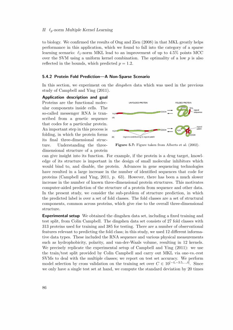
II `p-norm Multiple Kernel Learning
to biology. We confirmed the results of Ong and Zien (2008) in that MKL greatly helpsperformance in this application, which we found to fall into the category of a sparselearning scenario: `1-norm MKL lead to an improvement of up to 4.5% points MCCover the SVM using a uniform kernel combination. The optimality of a low p is alsoreflected in the bounds, which predicted p = 1.2.
5.4.2 Protein Fold Prediction—A Non-Sparse Scenario
In this section, we experiment on the dingshen data which was used in the previousstudy of Campbell and Ying (2011).
Figure 5.7: Figure taken from Alberts et al. (2002).
Application description and goalProteins are the functional molec-ular components inside cells. Theso-called messenger RNA is tran-scribed from a genetic sequencethat codes for a particular protein.An important step in this process isfolding, in which the protein formsits final three-dimensional struc-ture. Understanding the three-dimensional structure of a proteincan give insight into its function. For example, if the protein is a drug target, knowl-edge of its structure is important in the design of small molecular inhibitors whichwould bind to, and disable, the protein. Advances in gene sequencing technologieshave resulted in a large increase in the number of identified sequences that code forproteins (Campbell and Ying, 2011, p. 63). However, there has been a much slowerincrease in the number of known three-dimensional protein structures. This motivatescomputer-aided prediction of the structure of a protein from sequence and other data.In the present study, we consider the sub-problem of structure prediction, in whichthe predicted label is over a set of fold classes. The fold classes are a set of structuralcomponents, common across proteins, which give rise to the overall three-dimensionalstructure.
Experimental setup We obtained the dingshen data set, including a fixed training andtest split, from Colin Campbell. The dingshen data set consists of 27 fold classes with313 proteins used for training and 385 for testing. There are a number of observationalfeatures relevant to predicting the fold class; in this study, we used 12 different informa-tive data types. These included the RNA sequence and various physical measurementssuch as hydrophobicity, polarity, and van-der-Waals volume, resulting in 12 kernels.We precisely replicate the experimental setup of Campbell and Ying (2011): we usethe train/test split provided by Colin Campbell and carry out MKL via one-vs.-restSVMs to deal with the multiple classes; we report on test set accuracy. We performmodel selection by cross validation on the training set over C ∈ 10[−4,−3.5,...,4]. Sincewe only have a single test set at hand, we compute the standard deviation by 20 times
86
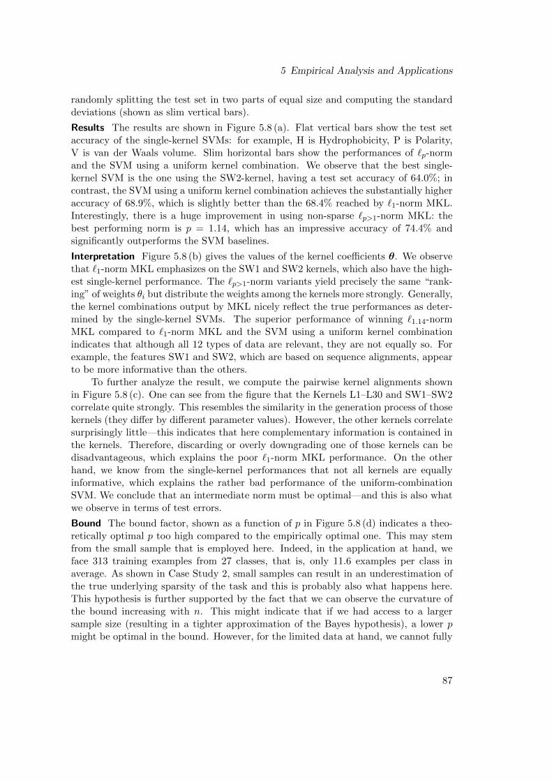
5 Empirical Analysis and Applications
randomly splitting the test set in two parts of equal size and computing the standarddeviations (shown as slim vertical bars).
Results The results are shown in Figure 5.8 (a). Flat vertical bars show the test setaccuracy of the single-kernel SVMs: for example, H is Hydrophobicity, P is Polarity,V is van der Waals volume. Slim horizontal bars show the performances of `p-normand the SVM using a uniform kernel combination. We observe that the best single-kernel SVM is the one using the SW2-kernel, having a test set accuracy of 64.0%; incontrast, the SVM using a uniform kernel combination achieves the substantially higheraccuracy of 68.9%, which is slightly better than the 68.4% reached by `1-norm MKL.Interestingly, there is a huge improvement in using non-sparse `p>1-norm MKL: thebest performing norm is p = 1.14, which has an impressive accuracy of 74.4% andsignificantly outperforms the SVM baselines.
Interpretation Figure 5.8 (b) gives the values of the kernel coefficients θ. We observethat `1-norm MKL emphasizes on the SW1 and SW2 kernels, which also have the high-est single-kernel performance. The `p>1-norm variants yield precisely the same “rank-ing” of weights θi but distribute the weights among the kernels more strongly. Generally,the kernel combinations output by MKL nicely reflect the true performances as deter-mined by the single-kernel SVMs. The superior performance of winning `1.14-normMKL compared to `1-norm MKL and the SVM using a uniform kernel combinationindicates that although all 12 types of data are relevant, they are not equally so. Forexample, the features SW1 and SW2, which are based on sequence alignments, appearto be more informative than the others.
To further analyze the result, we compute the pairwise kernel alignments shownin Figure 5.8 (c). One can see from the figure that the Kernels L1–L30 and SW1–SW2correlate quite strongly. This resembles the similarity in the generation process of thosekernels (they differ by different parameter values). However, the other kernels correlatesurprisingly little—this indicates that here complementary information is contained inthe kernels. Therefore, discarding or overly downgrading one of those kernels can bedisadvantageous, which explains the poor `1-norm MKL performance. On the otherhand, we know from the single-kernel performances that not all kernels are equallyinformative, which explains the rather bad performance of the uniform-combinationSVM. We conclude that an intermediate norm must be optimal—and this is also whatwe observe in terms of test errors.
Bound The bound factor, shown as a function of p in Figure 5.8 (d) indicates a theo-retically optimal p too high compared to the empirically optimal one. This may stemfrom the small sample that is employed here. Indeed, in the application at hand, weface 313 training examples from 27 classes, that is, only 11.6 examples per class inaverage. As shown in Case Study 2, small samples can result in an underestimation ofthe true underlying sparsity of the task and this is probably also what happens here.This hypothesis is further supported by the fact that we can observe the curvature ofthe bound increasing with n. This might indicate that if we had access to a largersample size (resulting in a tighter approximation of the Bayes hypothesis), a lower pmight be optimal in the bound. However, for the limited data at hand, we cannot fully
87
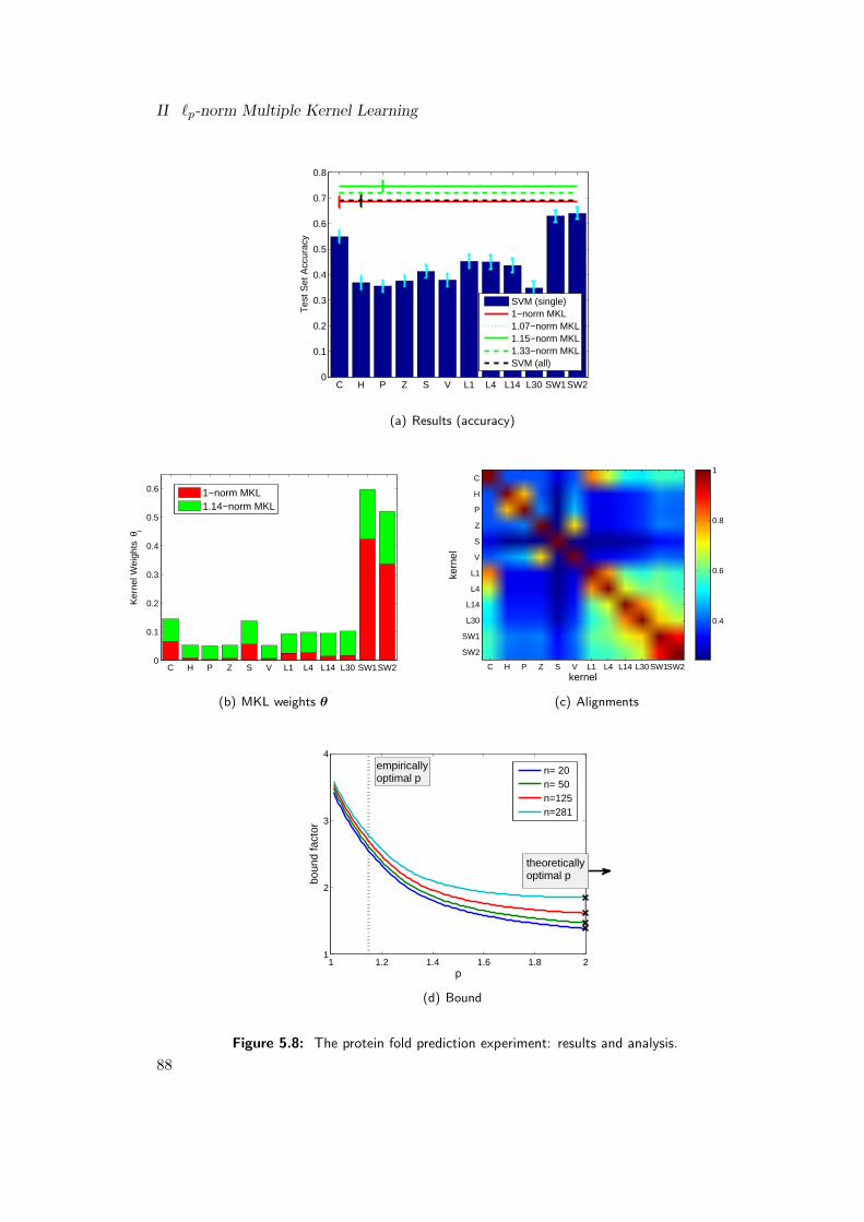
II `p-norm Multiple Kernel Learning
C H P Z S V L1 L4 L14 L30 SW1SW20
0.1
0.2
0.3
0.4
0.5
0.6
0.7
0.8
Tes
t Set
Acc
urac
y
SVM (single)1−norm MKL1.07−norm MKL1.15−norm MKL1.33−norm MKLSVM (all)
(a) Results (accuracy)
C H P Z S V L1 L4 L14 L30 SW1SW20
0.1
0.2
0.3
0.4
0.5
0.6
Ker
nel W
eigh
ts θ
i
1−norm MKL1.14−norm MKL
(b) MKL weights θ
kernel
kern
el
C H P Z S V L1 L4 L14 L30 SW1SW2
C
H
P
Z
S
V
L1
L4
L14
L30
SW1
SW2
0.4
0.6
0.8
1
(c) Alignments
1 1.2 1.4 1.6 1.8 21
2
3
4
p
boun
d fa
ctor
empiricallyoptimal p
n= 20n= 50n=125n=281
theoreticallyoptimal p
(d) Bound
Figure 5.8: The protein fold prediction experiment: results and analysis.
88
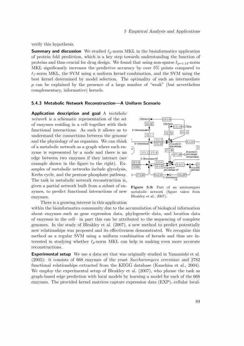
5 Empirical Analysis and Applications
verify this hypothesis.
Summary and discussion We studied `p-norm MKL in the bioinformatics applicationof protein fold prediction, which is a key step towards understanding the function ofproteins and thus crucial for drug design. We found that using non-sparse `p=1.14-normMKL significantly increases the predictive accuracy by over 5% points compared to`1-norm MKL, the SVM using a uniform kernel combination, and the SVM using thebest kernel determined by model selection. The optimality of such an intermediatep can be explained by the presence of a large number of “weak” (but neverthelesscomplementary, informative) kernels.
5.4.3 Metabolic Network Reconstruction—A Uniform Scenario
Figure 5.9: Part of an aminosugarsmetabolic network (figure taken fromBleakley et al., 2007).
Application description and goal A metabolicnetwork is a schematic representation of the setof enzymes residing in a cell together with theirfunctional interactions. As such it allows us tounderstand the connections between the genomeand the physiology of an organism. We can thinkof a metabolic network as a graph where each en-zyme is represented by a node and there is anedge between two enzymes if they interact (seeexample shown in the figure to the right). Ex-amples of metabolic networks include glycolysis,Krebs cycle, and the pentose phosphate pathway.The task in metabolic network reconstruction is,given a partial network built from a subset of en-zymes, to predict functional interactions of newenzymes.
There is a growing interest in this applicationwithin the bioinformatics community due to the accumulation of biological informationabout enzymes such as gene expression data, phylogenetic data, and location dataof enzymes in the cell—in part this can be attributed to the sequencing of completegenomes. In the study of Bleakley et al. (2007), a new method to predict potentiallynew relationships was proposed and its effectiveness demonstrated. We recognize thismethod as a regular SVM using a uniform combination of kernels and thus are in-terested in studying whether `p-norm MKL can help in making even more accuratereconstructions.
Experimental setup We use a data set that was originally studied in Yamanishi et al.(2005): it consists of 668 enzymes of the yeast Saccharomyces cerevisiae and 2782functional relationships extracted from the KEGG database (Kanehisa et al., 2004).We employ the experimental setup of Bleakley et al. (2007), who phrase the task asgraph-based edge prediction with local models by learning a model for each of the 668enzymes. The provided kernel matrices capture expression data (EXP), cellular local-
89
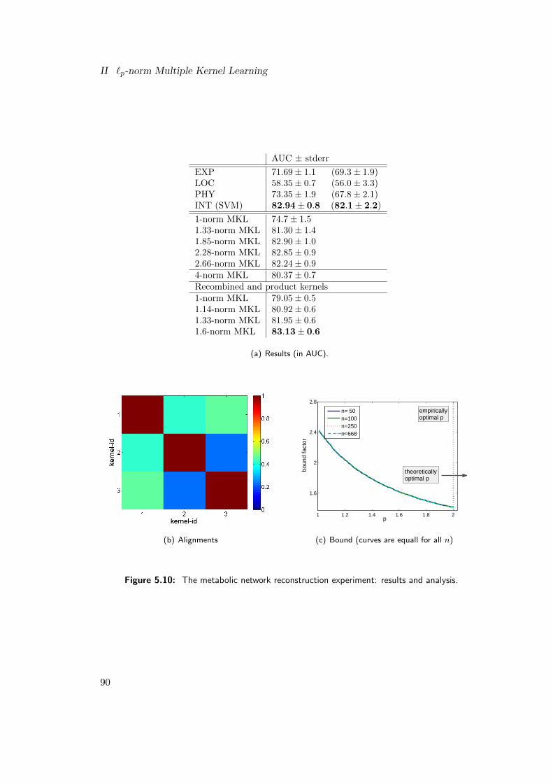
II `p-norm Multiple Kernel Learning
AUC ± stderr
EXP 71.69± 1.1 (69.3± 1.9)LOC 58.35± 0.7 (56.0± 3.3)PHY 73.35± 1.9 (67.8± 2.1)INT (SVM) 82.94± 0.8 (82.1± 2.2)
1-norm MKL 74.7± 1.51.33-norm MKL 81.30± 1.41.85-norm MKL 82.90± 1.02.28-norm MKL 82.85± 0.92.66-norm MKL 82.24± 0.94-norm MKL 80.37± 0.7Recombined and product kernels1-norm MKL 79.05± 0.51.14-norm MKL 80.92± 0.61.33-norm MKL 81.95± 0.61.6-norm MKL 83.13± 0.6
(a) Results (in AUC).
(b) Alignments
1 1.2 1.4 1.6 1.8 2
1.6
2
2.4
2.8
p
boun
d fa
ctor
empiricallyoptimal p
n= 50n=100n=250n=668
theoreticallyoptimal p
(c) Bound (curves are equall for all n)
Figure 5.10: The metabolic network reconstruction experiment: results and analysis.
90
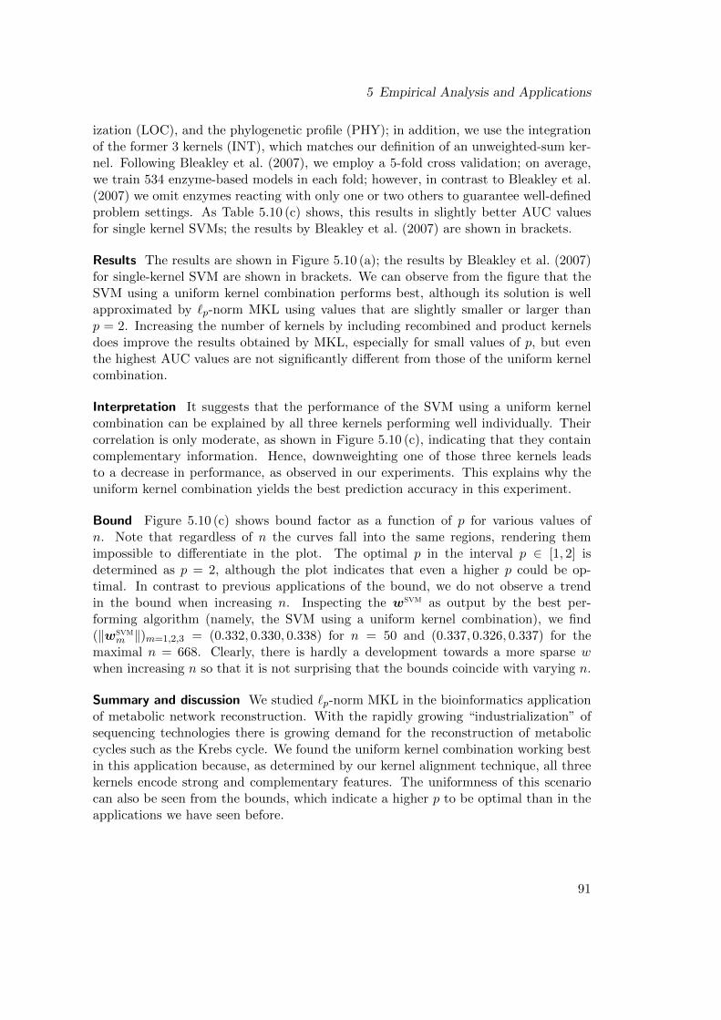
5 Empirical Analysis and Applications
ization (LOC), and the phylogenetic profile (PHY); in addition, we use the integrationof the former 3 kernels (INT), which matches our definition of an unweighted-sum ker-nel. Following Bleakley et al. (2007), we employ a 5-fold cross validation; on average,we train 534 enzyme-based models in each fold; however, in contrast to Bleakley et al.(2007) we omit enzymes reacting with only one or two others to guarantee well-definedproblem settings. As Table 5.10 (c) shows, this results in slightly better AUC valuesfor single kernel SVMs; the results by Bleakley et al. (2007) are shown in brackets.
Results The results are shown in Figure 5.10 (a); the results by Bleakley et al. (2007)for single-kernel SVM are shown in brackets. We can observe from the figure that theSVM using a uniform kernel combination performs best, although its solution is wellapproximated by `p-norm MKL using values that are slightly smaller or larger thanp = 2. Increasing the number of kernels by including recombined and product kernelsdoes improve the results obtained by MKL, especially for small values of p, but eventhe highest AUC values are not significantly different from those of the uniform kernelcombination.
Interpretation It suggests that the performance of the SVM using a uniform kernelcombination can be explained by all three kernels performing well individually. Theircorrelation is only moderate, as shown in Figure 5.10 (c), indicating that they containcomplementary information. Hence, downweighting one of those three kernels leadsto a decrease in performance, as observed in our experiments. This explains why theuniform kernel combination yields the best prediction accuracy in this experiment.
Bound Figure 5.10 (c) shows bound factor as a function of p for various values ofn. Note that regardless of n the curves fall into the same regions, rendering themimpossible to differentiate in the plot. The optimal p in the interval p ∈ [1, 2] isdetermined as p = 2, although the plot indicates that even a higher p could be op-timal. In contrast to previous applications of the bound, we do not observe a trendin the bound when increasing n. Inspecting the wsvm as output by the best per-forming algorithm (namely, the SVM using a uniform kernel combination), we find(‖wsvm
m ‖)m=1,2,3 = (0.332, 0.330, 0.338) for n = 50 and (0.337, 0.326, 0.337) for themaximal n = 668. Clearly, there is hardly a development towards a more sparse wwhen increasing n so that it is not surprising that the bounds coincide with varying n.
Summary and discussion We studied `p-norm MKL in the bioinformatics applicationof metabolic network reconstruction. With the rapidly growing “industrialization” ofsequencing technologies there is growing demand for the reconstruction of metaboliccycles such as the Krebs cycle. We found the uniform kernel combination working bestin this application because, as determined by our kernel alignment technique, all threekernels encode strong and complementary features. The uniformness of this scenariocan also be seen from the bounds, which indicate a higher p to be optimal than in theapplications we have seen before.
91
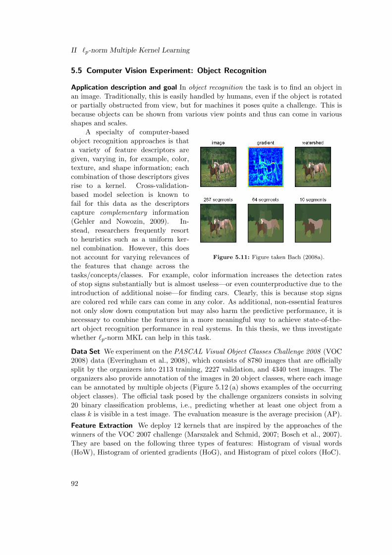
II `p-norm Multiple Kernel Learning
5.5 Computer Vision Experiment: Object Recognition
Application description and goal In object recognition the task is to find an object inan image. Traditionally, this is easily handled by humans, even if the object is rotatedor partially obstructed from view, but for machines it poses quite a challenge. This isbecause objects can be shown from various view points and thus can come in variousshapes and scales.
Figure 5.11: Figure taken Bach (2008a).
A specialty of computer-basedobject recognition approaches is thata variety of feature descriptors aregiven, varying in, for example, color,texture, and shape information; eachcombination of those descriptors givesrise to a kernel. Cross-validation-based model selection is known tofail for this data as the descriptorscapture complementary information(Gehler and Nowozin, 2009). In-stead, researchers frequently resortto heuristics such as a uniform ker-nel combination. However, this doesnot account for varying relevances ofthe features that change across thetasks/concepts/classes. For example, color information increases the detection ratesof stop signs substantially but is almost useless—or even counterproductive due to theintroduction of additional noise—for finding cars. Clearly, this is because stop signsare colored red while cars can come in any color. As additional, non-essential featuresnot only slow down computation but may also harm the predictive performance, it isnecessary to combine the features in a more meaningful way to achieve state-of-the-art object recognition performance in real systems. In this thesis, we thus investigatewhether `p-norm MKL can help in this task.
Data Set We experiment on the PASCAL Visual Object Classes Challenge 2008 (VOC2008) data (Everingham et al., 2008), which consists of 8780 images that are officiallysplit by the organizers into 2113 training, 2227 validation, and 4340 test images. Theorganizers also provide annotation of the images in 20 object classes, where each imagecan be annotated by multiple objects (Figure 5.12 (a) shows examples of the occurringobject classes). The official task posed by the challenge organizers consists in solving20 binary classification problems, i.e., predicting whether at least one object from aclass k is visible in a test image. The evaluation measure is the average precision (AP).
Feature Extraction We deploy 12 kernels that are inspired by the approaches of thewinners of the VOC 2007 challenge (Marszalek and Schmid, 2007; Bosch et al., 2007).They are based on the following three types of features: Histogram of visual words(HoW), Histogram of oriented gradients (HoG), and Histogram of pixel colors (HoC).
92
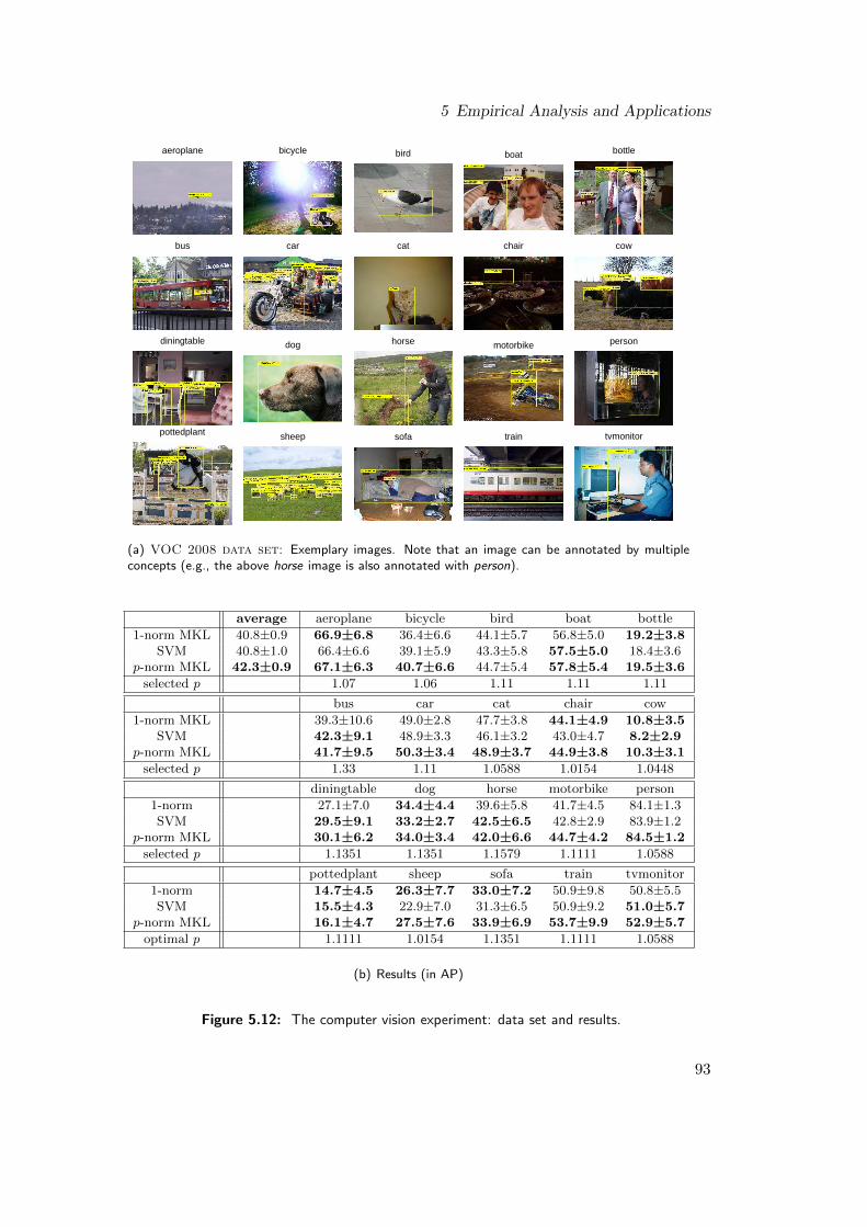
5 Empirical Analysis and Applications
aeroplane bicycle bird boat bottle
bus car cat chair cow
diningtable dog horse motorbike person
pottedplant sheep sofa train tvmonitor
(a) VOC 2008 data set: Exemplary images. Note that an image can be annotated by multipleconcepts (e.g., the above horse image is also annotated with person).
average aeroplane bicycle bird boat bottle
1-norm MKL 40.8±0.9 66.9±6.8 36.4±6.6 44.1±5.7 56.8±5.0 19.2±3.8SVM 40.8±1.0 66.4±6.6 39.1±5.9 43.3±5.8 57.5±5.0 18.4±3.6
p-norm MKL 42.3±0.9 67.1±6.3 40.7±6.6 44.7±5.4 57.8±5.4 19.5±3.6
selected p 1.07 1.06 1.11 1.11 1.11
bus car cat chair cow
1-norm MKL 39.3±10.6 49.0±2.8 47.7±3.8 44.1±4.9 10.8±3.5SVM 42.3±9.1 48.9±3.3 46.1±3.2 43.0±4.7 8.2±2.9
p-norm MKL 41.7±9.5 50.3±3.4 48.9±3.7 44.9±3.8 10.3±3.1
selected p 1.33 1.11 1.0588 1.0154 1.0448
diningtable dog horse motorbike person
1-norm 27.1±7.0 34.4±4.4 39.6±5.8 41.7±4.5 84.1±1.3SVM 29.5±9.1 33.2±2.7 42.5±6.5 42.8±2.9 83.9±1.2
p-norm MKL 30.1±6.2 34.0±3.4 42.0±6.6 44.7±4.2 84.5±1.2
selected p 1.1351 1.1351 1.1579 1.1111 1.0588
pottedplant sheep sofa train tvmonitor
1-norm 14.7±4.5 26.3±7.7 33.0±7.2 50.9±9.8 50.8±5.5SVM 15.5±4.3 22.9±7.0 31.3±6.5 50.9±9.2 51.0±5.7
p-norm MKL 16.1±4.7 27.5±7.6 33.9±6.9 53.7±9.9 52.9±5.7
optimal p 1.1111 1.0154 1.1351 1.1111 1.0588
(b) Results (in AP)
Figure 5.12: The computer vision experiment: data set and results.
93
II `p-norm Multiple Kernel Learning
1. The HoW features are constructed in a standard way as in Csurka et al. (2004):first, the SIFT descriptors (Lowe, 2004) are calculated on a grid of 10 pixel pitchesfor each image using a code book of size 1200, which is learned by k-means clusteringdeploying the SIFT descriptors extracted from the training images. Then, all SIFTdescriptors are assigned to visual words (prototypes) and summarized into histogramswithin entire images or sub-regions, deploying HoW features over the grey and huechannels.
2. The HoG features over the grey channel are computed by discretizing the orientationof the gradient vector at each pixel into 40 bins and by summarizing the discretizedorientations into histograms within image regions (Dalal and Triggs, 2005; Bosch et al.,2007). Canny detectors (Canny, 1986) are used to discard contributions from pixels,around which the image is almost uniform.
3. The HoC features over the hue channel are constructed by pixel-wise discretizingcolor values and computing their histograms within image regions.
The above features are histograms containing no spatial information. We thereforeenrich the respective representations by a pyramidal approach (Lazebnik et al., 2006)to also capture the spatial context of an image. Furthermore, we apply a χ2 kernel(Zhang et al., 2007) on top of the enriched histogram features, where the bandwidth ofthe χ2 kernel is heuristically chosen (proportional to the mean of the squared Euclideandistance averaged over all training example pairs (Lampert and Blaschko, 2008)). Intotal, we prepared 12 kernels by mutually combining 4 feature types/colors HoWg,HoWh, HoGg, HoCh with 3 pyramid levels. All kernels were spherically normalizedaccording to Eq. (3.7).
Experimental setup The original data set contains a test set, but with the labelsbeing undisclosed. We therefore create 10 random splits of the unified training andvalidation sets into new, smaller sets containing 2111 training, 1111 validation, and1110 test images. For each of the 10 splits, the training images are used for learningclassifiers, while the SVM regularization parameter C and the MKL norm parameterp are chosen based on the maximal AP score on the validation images. Thereby, theregularization constant C and the norm parameter p are optimized class-wise from thecandidates 2−4, 2−3, . . . , 24.
For a thorough evaluation, we would have to construct another codebook for eachcross-validation split. However, creating codebooks and assigning descriptors to visualwords is a time-consuming process. In our experiments, we therefore resort to thecommon practice of using a single codebook created from all training images containedin the official split. Although this could result in a slight overestimation of the APscores, this affects all methods equally and does not favor any classification methodover another—our focus lies on a relative comparison of the different classificationmethods; therefore there is no loss in exploiting this computational shortcut.
Note that we exclude a comparison to single-kernel SVMs since it is clear for thisapplication that a single kernel alone cannot capture the relevant information neededfor this task (see, e.g., Gehler and Nowozin, 2009, and references therein).
94
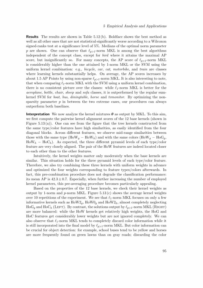
5 Empirical Analysis and Applications
Results The results are shown in Table 5.12 (b). Boldface shows the best method aswell as all other ones that are not statistical-significantly worse according to a Wilcoxonsigned-ranks test at a significance level of 5%. Medians of the optimal norm parameterp are shown. One can observe that `p>1-norm MKL is among the best algorithmsindependent of the concept class, except for bird where it attains the maximal APscore, but insignificantly so. For many concepts, the AP score of `p>1-norm MKLis considerably higher than the one attained by 1-norm MKL or the SVM using theuniform kernel combination: e.g., bicycle, car, cat, motorbike, and train are classeswhere learning kernels substantially helps. On average, the AP scores increases byabout 1.5 AP Points by using non-sparse `p>1-norm MKL. It is also interesting to note,that when comparing `1-norm MKL with the SVM using a uniform kernel combination,there is no consistent picture over the classes: while `1-norm MKL is better for theaeroplane, bottle, chair, sheep and sofa classes, it is outperformed by the regular sum-kernel SVM for boat, bus, diningtable, horse and tvmonitor. By optimizing the non-sparsity parameter p in between the two extreme cases, our procedures can alwaysoutperform both baselines.
Interpretation We now analyze the kernel mixtures θ as output by MKL. To this aim,we first compute the pairwise kernel alignment scores of the 12 base kernels (shown inFigure 5.13 (a)). One can see from the figure that the tree kernels constructed fromthe same type/color features have high similarities, as easily identified from the fourdiagonal blocks. Across different features, we observe mid-range similarities betweenthose with the same type (HoWg − HoWh) and with the same colors (HoWg − HoGg,HoWh − HoCh). As expected, the three different pyramid levels of each type/colorfeature are very closely aligned. The pair of the HoW features are indeed located closerto each other than to the other features.
Intuitively, the kernel weights matter only moderately when the base kernels aresimilar. This situation holds for the three pyramid levels of each type/color feature.Therefore, we also try combining these three kernels with uniform weights in advanceand optimized the four weights corresponding to feature types/colors afterwards. Infact, this pre-combination procedure does not degrade the classification performance:its mean AP is 42.3± 0.7. Especially, when further increasing the number of employedkernel parameters, this pre-averaging procedure becomes particularly appealing.
Based on the properties of the 12 base kernels, we check their kernel weights asoutput by 1-norm and p-norm MKL. Figure 5.13 (c) shows the average kernel weightsover 10 repetitions of the experiment. We see that `1-norm MKL focuses on only a fewinformative kernels such as HoW2g, HoW0g and HoW2h, almost completely neglectingHoGg and HoCh (Left). By contrast, the solutions output by `p>1-norm MKL (Right)are more balanced: while the HoW kernels get relatively high weights, the HoG andHoC features get considerably lower weights but are not ignored completely. We canalso observe that `1-norm MKL tends to completely discard color information while itis still incorporated into the final model by `p>1-norm MKL. But color information canbe crucial for object detection: for example, school buses tend to be yellow and horsesare more frequently found on green lawns than on gray roads; discarding the color
95
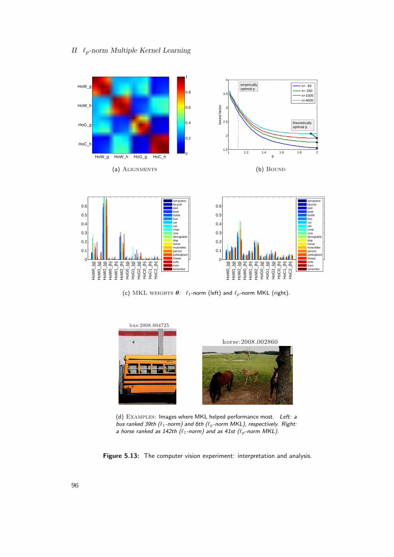
II `p-norm Multiple Kernel Learning
HoW_g HoW_h HoG_g HoC_h
HoW_g
HoW_h
HoG_g
HoC_h
0
0.2
0.4
0.6
0.8
1
(a) Alignments
1 1.2 1.4 1.6 1.8 21.5
2
2.5
3
3.5
4
p
boun
d fa
ctor
empiricallyoptimal p
n= 60n= 260n=1000n=4000
theoreticallyoptimal p
(b) Bound
0
0.1
0.2
0.3
0.4
0.5
0.6
HoW
0_g
H
oW1_
g
HoW
2_g
H
oW0_
h
HoW
1_h
H
oW2_
h
HoG
0_g
H
oG1_
g
HoG
2_g
H
oC0_
h
HoC
1_h
H
oC2_
h
aeroplanebicyclebirdboatbottlebuscarcatchaircowdiningtabledoghorsemotorbikepersonpottedplantsheepsofatraintvmonitor
0
0.1
0.2
0.3
0.4
0.5
0.6
HoW
0_g
H
oW1_
g
HoW
2_g
H
oW0_
h
HoW
1_h
H
oW2_
h
HoG
0_g
H
oG1_
g
HoG
2_g
H
oC0_
h
HoC
1_h
H
oC2_
h
aeroplanebicyclebirdboatbottlebuscarcatchaircowdiningtabledoghorsemotorbikepersonpottedplantsheepsofatraintvmonitor
(c) MKL weights θ: `1-norm (left) and `p-norm MKL (right).
bus:2008 004725
horse:2008 002860
(d) Examples: Images where MKL helped performance most. Left: abus ranked 39th (`1-norm) and 6th (`p-norm MKL), respectively. Right:a horse ranked as 142th (`1-norm) and as 41st (`p-norm MKL).
Figure 5.13: The computer vision experiment: interpretation and analysis.
96
5 Empirical Analysis and Applications
information, as done by `1-norm MKL, hurts performance on concept classes that arewell characterized by colors—this might be one of the major reasons for the superiorperformance of `p-norm MKL on these images compared to the `1-norm MKL.
Figure 5.13 (d) shows example images where `p-norm MKL greatly helps general-ization performance. In both cases, `1-norm MKL tends to focus on the finest pyramidlayer, and tries to capture layout information. However, since the VOC dataset includesa substantial number of not-so-well-aligned images (such as the examples shown in thefigure), focusing on layout might sometimes fail. In contrast, `p-norm MKL distributesmore weights to coarser pyramid layers, and thus successfully identifies these images.
Bound From the bound shown in Figure 5.13 (b), we observe an overestimation ofthe optimal p. The empirical best p was p = 1.11 in median. In contrast, the boundpredicts a p with p ≈ 2. This is very similar to what be have already observed inthe protein fold prediction experiment, presented in Section 5.4.2. Interestingly, bothexperiments, the present one and the protein folding experiment, consist of multi-labelclassification tasks with 20 and 27 classes, respectively. This indicates that, for small n,the bounds are not reliable in multi-label classification problems. Nevertheless, we canobserve a trend towards a more accurate prediction of the optimal p with increasing n,which is similar to the previous experiments. It could thus be conjectured that withincreasing n the bound’s prediction will eventually coincide with what is also measuredempirically.
Summary and discussion In this chapter, we applied `p-norm MKL to object recogni-tion in computer vision. While humans can easily recognize objects in images, even ifthey are rotated or partly covered, machines frequently fail in this task. Since imagesare characterized by heterogeneous kernels arising from color, texture, or shape infor-mation, but the usefulness of a particular kernel strongly depends on the object to bediscovered (for example, cows are frequently found in front of green lawns while carscan come in any color), it is very appealing to use MKL in this application. Indeed,in our experiments on the official VOC08 challenge data set, we observed a substantialimprovement in using `p-norm MKL—this holds over the whole range of object classes.Using the alignment technique we connected this fact with the color information be-ing discarded by `1-norm MKL while it is overly incorporated into the uniform kernelcombination. This is especially remarkable since the uniform SVM was shown to be atough competitor in the past (Gehler and Nowozin, 2009). The latter might also beconnected with prior knowledge that is incorporated by researchers when the set ofkernels is chosen a priori.
5.6 Summary and Discussion
We empirically analyzed the generalization performance of `p-norm MKL in terms ofthe test error and application-specific evaluation measures, respectively. To this end,we measured the accuracy of `p-norm MKL and compared it to the one achieved bythe SVM baselines, using either a uniform kernel combination or a single kernel tunedby model selection. To analyze the results we developed a methodology based on
97
II `p-norm Multiple Kernel Learning
theoretical bounds (investigating the theoretically optimal p) and kernel alignments(analyzing the complementariness of the kernel set). We exemplified the methodologyby means of a toy experiment, where we constructed data by gradually increasingthe true underlying sparsity (as measured by the size of the sparsity pattern of theBayes hypothesis), resulting in several constructed learning scenario that differ in theirunderlying sparsity. First, we observed the theoretical bounds reflecting the empiricallyobserved optimal p in the idealized setup where we know the Bayes hypothesis; second,we showed that kernel alignments reflect the dependancy structure of the kernel set;third, we found that the choice of the norm parameter p can be crucial to obtain a hightest set accuracy, concluding that in the presence of many irrelevant kernels, a smallp is expected to be beneficial and an intermediate/large p will prove to be beneficialotherwise.
We then applied `p-norm MKL to diverse, highly topical and challenging prob-lems from the domains of bioinformatics and computer vision on small and large scales.Data frequently arises in those domains from multiple heterogeneous sources or is repre-sented by various complementary views, the right combination of which being unknown,rendering them especially appealing for the use of MKL. Beside investigating the ef-fectiveness of `p-norm MKL in terms of test set accuracy, we were also interested inunderstanding the results, implementing the proposed methodology.
We exemplarily carried out the proposed experimental methodology for transcrip-tion start site detection, a cutting-edge bioinformatics application. The data set weexperimented on was also used in the previous study of Sonnenburg et al. (2006a) andcomprises 93,500 instances. We showed that regardless of the sample size, `p-normMKL can improve the prediction accuracy over `1-norm MKL and the SVM using auniform kernel combination (which itself outperforms the single-kernel SVM using thekernel determined by model selection). This is remarkable and of significance for theapplication domain: the method using a uniform kernel combination was recently con-firmed to be the most accurate TSS detector in a comparison of 19 state-of-the-artmodels Abeel et al. (2009). Furthermore, we observed that the choice of n had noimpact on the empirical optimality of a particular p. We also evaluated the theoreticalbounds and found that with increasing n they give a more and more accurate estimationof the optimal p through an increasingly tight approximation of the Bayes hypothesis.
Moreover, we also studied other applications from the domain of bioinformatics:protein subcellular localization, protein fold prediction, and metabolic network recon-struction. In a nutshell, we found this domain being too diverse to be categorized intoa single learning scenario (e.g., sparse). In fact, we presented diverse bioinformaticsapplications covering the whole range of scenarios: sparse, intermediate non-sparse,and uniform. However, by appropriately tuning the norm parameter, `p-norm MKLproved robust in all scenarios.
Finally, we applied `p-norm MKL to object recognition, a burning topic in com-puter vision. The same setting was also studied earlier by Varma and Ray (2007) andGehler and Nowozin (2009), who found classical MKL to not increase the predictionaccuracy compared to the uniform kernel SVM baseline. We applied the developed `p-
98

5 Empirical Analysis and Applications
norm MKL to this application domain and showed that, by taking p = 1.11 in median,the prediction accuracy could be raised over the SVM baselines, regardless of the objectclass, by an AP score of 1.5 in average, and for 7 out of the 20 classes significantly so.
99

Conclusion and Outlook
To successfully cope with the most recent challenges imposed by application domainssuch as bioinformatics and computer vision, machine learning systems need to effec-tively deal with the multiple data representations—or kernels—naturally arising inthose domains. Previous approaches to learning with multiple kernels restrict the searchspace by convex combinations, promoting sparse solutions to support interpretabilityand scalability. Unfortunately, this is often too restrictive and hinders MKL beingeffective in practice, as demonstrated in a variety of recent works (e.g. Cortes et al.,2008; Gehler and Nowozin, 2008; Kloft et al., 2008b; Noble, 2008; Cortes, 2009; Gehlerand Nowozin, 2009; Kloft et al., 2009a).
In this thesis, we addressed the problem of learning with multiple kernels by propos-ing the `p-norm multiple kernel learning methodology, deduced from a rigorous math-ematical framework for learning with multiple kernels, unifying previous approachesto learning with multiple kernels under a common umbrella. In an extensive study,we evaluated `p-norm multiple kernel learning empirically in controlled environmentsas well as in highly topical real-work applications from the domains of computer vi-sion and bioinformatics, comparing our methodology to even its strongest competitorssuch as the support vector machine using a uniform kernel combination. We found`p-norm multiple kernel learning being more efficient and more accurate than previousapproaches to learning with multiple kernels, allowing us to deal with up to ten thou-sands of data points and thousands of kernels at the same time, as demonstrated onseveral data sets.
Our methodology is underpinned by deep foundations in the theory of learning:we proved tight lower and upper bounds on the complexity of the hypothesis classassociated with `p-norm multiple kernel learning, giving theoretical guarantees on thefit of our method and showing that, depending on the true underlying learning task,our framework can attain stronger theoretical guarantees than classical approaches tolearning with multiple kernels. Stimulated by recent attempts to catalyze research inthe direction of understanding learning with multiple kernels (Lanckriet et al., 2009), weshowed that the optimality of `p-norm multiple kernel learning can be connected withthe stronger theoretical guarantees that it attains in practice, compared to classicalapproaches.
The proposed framework does not generally require the incorporation of expertknowledge; however, such application-specific knowledge can be used to further improveits performance, for example, by pre-selecting or upscaling kernels with high informationcontent. In combination with this technique, `p-norm multiple kernel learning can evencope with the most challenging problems posed by application domains.
101
II `p-norm Multiple Kernel Learning
Summary of Results
The main results of this thesis can be summarized as follows.
Chapter 2. We presented a mathematical framework for learning with multiplekernels, comprising most existing lines of research in that area and rigorously gener-alizing the classic approach of Bach et al. (2004). We unified previous formulationsunder a common umbrella, which allowed us to analyze a large variety of MKL meth-ods jointly, as exemplified by deriving a general dual representation of the criterion,without making assumptions on the employed norms and losses, beside the latter beingconvex. This delivered insights into connections between existing MKL formulationsand, even more importantly, can be used to derive novel MKL formulations as specialcases of the framework.
Chapter 3. We derived efficient algorithms to solve the `p-norm MKL optimizationproblem. All algorithms, for the sake of performance, are implemented in C++, but forusability, are equipped with interfaces to MATLAB, Octave, Phyton, and R. We alsowrote macro scripts completely automating the whole process from training over modelselection to evaluation. Our software is freely available under the GPL license. In ourcomputational experiments, we found these large-scale optimization algorithms allowingus to deal with ten thousands of data points and thousands of kernels at the sametime, as demonstrated on the MNIST data set. We compared our algorithms to thestate-of-the-art in MKL research, namely HessianMKL (Chapelle and Rakotomamonjy,2008) and SimpleMKL (Rakotomamonjy et al., 2008), and found ours to be up to twomagnitudes faster. We proved the convergence of our AnalyticalMKL using the usualregularity assumptions.
Chapter 4. The proposed techniques are also theoretically founded: we provedtight lower and upper bounds on the local and global Rademacher complexities ofthe hypothesis class associated with `p-norm MKL, from which we derived excess riskbounds with fast convergence rates, thus being tighter than existing bounds for `p-norm MKL (Cortes et al., 2010a), which only achieved slow convergence rates. Whilefor our results to hold we employed an assumption on the independence of the kernels,related works on sparse recovery required similar assumptions (Raskutti et al., 2010;Koltchinskii and Yuan, 2010). We connected the minimal values of the bounds withthe structured soft sparsity of the underlying Bayes hypothesis, demonstrating thatfor a large range of learning scenarios `p-norm MKL attains substantially strongergeneralization guarantees than classical MKL, justifying the use of `p-norm MKL andmultiple kernel learning in general.
Chapter 5. In an extensive evaluation, we empirically measured the generaliza-tion performance of `p-norm MKL on diverse and relevant real-world applications frombioinformatics and computer vision. We developed a methodology based on the theoret-ical bounds and kernel alignments for analyzing the results, as exemplified by means ofa toy experiment, where we observed the theoretical bounds and the kernel alignmentswell reflecting the empirically observed optimal p. We carried out the experimentalmethodology for genomic transcription start site detection. We showed that regardless
102
5 Empirical Analysis and Applications
of the sample size, by taking p = 4/3, `p-norm MKL can improve the prediction ac-curacy over `1-norm MKL and SVM using a uniform kernel combination, which wasrecently confirmed to be the most accurate TSS detector in an international compar-ison of 19 models Abeel et al. (2009). We also evaluated the theoretical bounds andfound them with increasing n increasingly accurate reflecting the optimal p. We ap-plied `p-norm MKL to protein fold prediction, achieving an significant improvementof 6% in accuracy. Finally, we applied `p-norm MKL to object recognition, a burningtopic in computer vision, studied earlier by Varma and Ray (2007) and Gehler andNowozin (2009) who found no improvement in using classical MKL. In contrast, weshowed that, by taking p = 1.11 in median, `p-norm MKL outperforms even the bestSVM competitors, regardless of the object class.
Future Work
As recently argued in Kloft et al. (2010b), among the most important challenges inmultiple kernel learning is the exploration of new objectives and parameterizations.To this end, an interesting approach was recently undertaken by Yan et al. (2010),who studied a `2-norm MKL variant based on a Fisher discriminant objective functionwith very promising results on object categorization tasks. Similar objectives werealso explored in Yu et al. (2010), who presented a more general formulation. Firststeps towards new ways of combining kernels were undertaken in Varma and Babu(2009) and Cortes et al. (2009b), respectively, where non-linear combinations (productsand polynomials, respectively) were studied. Unfortunately, in the current state ofresearch, both formulations in general lead to non-convex optimization problems andthe corresponding objectives are hard to optimize accurately.
Besides classification, which forms the core of machine learning and on which wefocused in this thesis, it is interesting to study the proposed methodology also in otherlearning tasks such as regression or novelty detection tasks. A first step in this directionwas undertaken in Cortes et al. (2009a), where `p-norm MKL was applied to regressiontasks on Reuters and various sentiment analysis datasets, but restricted to the casep = 4/3. Here it would be interesting to exploit the full power of our framework bystudying the whole range of p ∈ [1,∞]. Another approach towards different learningtasks was undertaken in Kloft et al. (2009b), where density-level set estimation andnovelty detection were studied with promising first results. Likewise, semi-supervisedlearning (Chapelle et al., 2006) is to be explored. Also, online learning recently gainedconsiderable attention (Orabona et al., 2010) and is subject to current work (Martinset al., 2011; Orabona and Jie, 2011).
Future work could also aim at further exploring applications of `p-norm MKL.Ongoing work in the field of computer vision is based on Nakajima et al. (2009b), in-vestigating `p-norm multiple kernel learning on photo annotation tasks with promisingfirst results. Also, effectively learning taxonomies (Binder et al., 2011) has recentlygained attention from the scientific community and could benefit from the use of MKL.Also, in the bioinformatics domain, we observed applications of `p-norm MKL, most
103
II `p-norm Multiple Kernel Learning
notably, the study by Yu et al. (2010) on two real-world genomic data sets for clinicaldecision support in cancer diagnosis and disease relevant gene prioritization, respec-tively, showing a substantial improvement in using `4/3-norm MKL compared to theSVM baselines. Again, it would be interesting to refine the analysis by searching for anoptimal p and, moreover, evaluate our bounds and kernel alignments. Another interest-ing application is computer security, where MKL was successfully applied to networkintrusion detection tasks (Kloft et al., 2008a), using appropriate loss functions.
It would also be interesting to further theoretically explore the `p-norm multiplekernel learning framework, for example, beyond the traditional borders of the localRademacher complexities. Clearly, future work here could built upon Bartlett andMendelson (2006). Another theoretical challenge is to analyze more complex hypothesisclasses. The unifying framework presented in this thesis might serve as a good startingpoint for such an undertaking, as exemplified for the case of generalized elastic-net-style classes in Kloft et al. (2010a). This is becoming especially pressing with respectto non-isotropic hypothesis classes that might also be profitable in practice since theyallow for the incorporation of expert knowledge. A considerable amount of work onthose non-standard classes would also have to focus on optimization algorithms.
Finally, an innovative approach was recently taken in Widmer et al. (2010), where`p>1-norm MKL was exploited as a methodical tool to learn hierarchy structures inmulti-task learning, thus extending the work of Evgeniou and Pontil (2004) to thestructured domain. This indicates the many possibilities for further exploration of ourframework beyond the standard setting, for example, exploring the relations to learningdistance metrics or learning the covariance function of a Gaussian process—clearly, thisrequires research that goes beyond the classical setup.
104
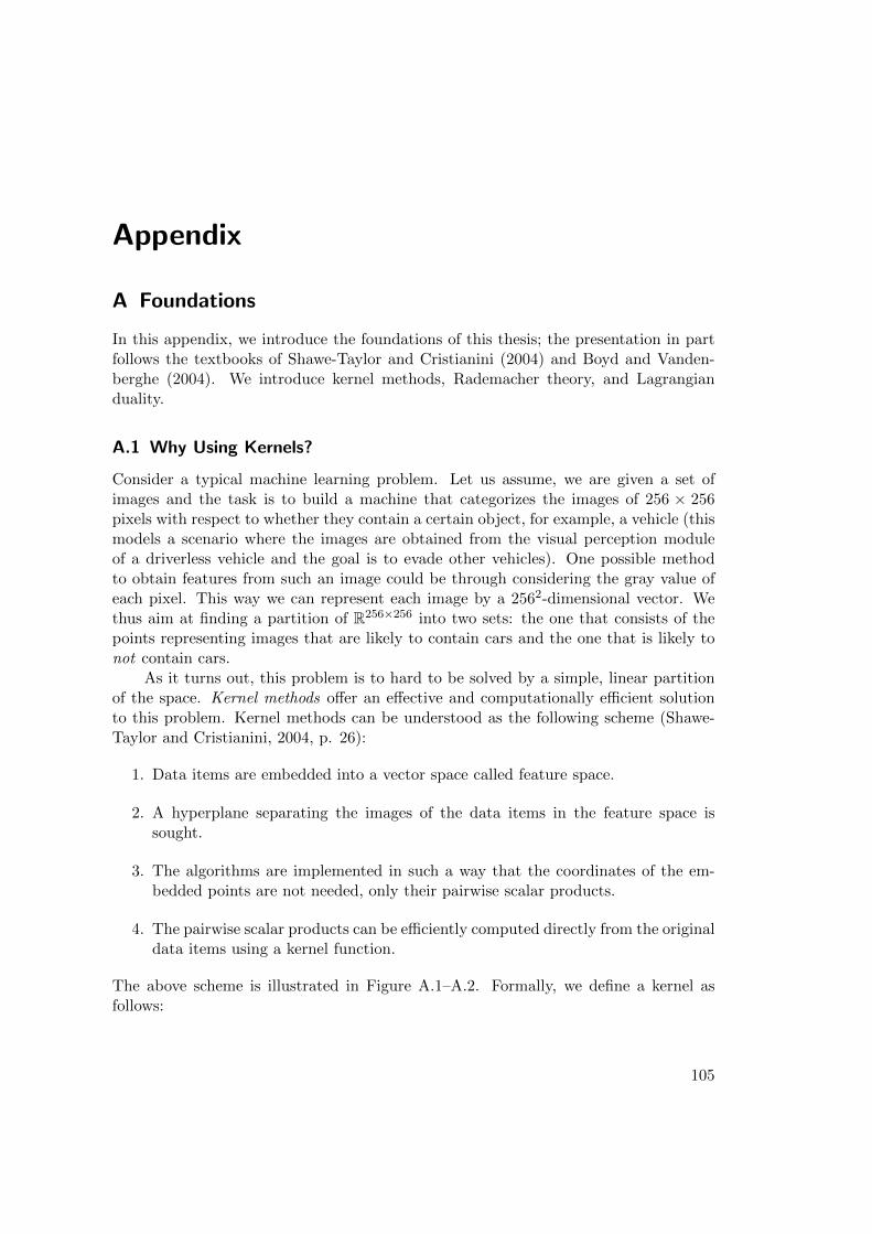
Appendix
A Foundations
In this appendix, we introduce the foundations of this thesis; the presentation in partfollows the textbooks of Shawe-Taylor and Cristianini (2004) and Boyd and Vanden-berghe (2004). We introduce kernel methods, Rademacher theory, and Lagrangianduality.
A.1 Why Using Kernels?
Consider a typical machine learning problem. Let us assume, we are given a set ofimages and the task is to build a machine that categorizes the images of 256 × 256pixels with respect to whether they contain a certain object, for example, a vehicle (thismodels a scenario where the images are obtained from the visual perception moduleof a driverless vehicle and the goal is to evade other vehicles). One possible methodto obtain features from such an image could be through considering the gray value ofeach pixel. This way we can represent each image by a 2562-dimensional vector. Wethus aim at finding a partition of R256×256 into two sets: the one that consists of thepoints representing images that are likely to contain cars and the one that is likely tonot contain cars.
As it turns out, this problem is to hard to be solved by a simple, linear partitionof the space. Kernel methods offer an effective and computationally efficient solutionto this problem. Kernel methods can be understood as the following scheme (Shawe-Taylor and Cristianini, 2004, p. 26):
1. Data items are embedded into a vector space called feature space.
2. A hyperplane separating the images of the data items in the feature space issought.
3. The algorithms are implemented in such a way that the coordinates of the em-bedded points are not needed, only their pairwise scalar products.
4. The pairwise scalar products can be efficiently computed directly from the originaldata items using a kernel function.
The above scheme is illustrated in Figure A.1–A.2. Formally, we define a kernel asfollows:
105
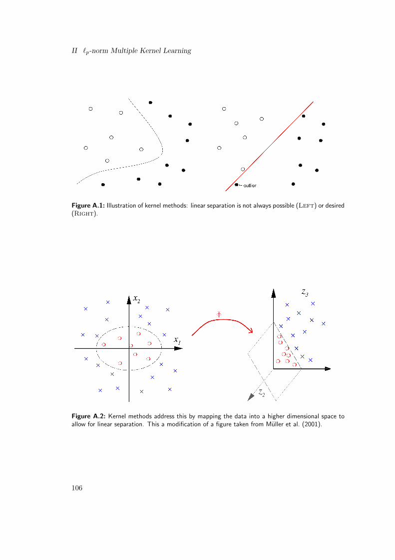
II `p-norm Multiple Kernel Learning
Figure A.1: Illustration of kernel methods: linear separation is not always possible (Left) or desired(Right).
Figure A.2: Kernel methods address this by mapping the data into a higher dimensional space toallow for linear separation. This a modification of a figure taken from Muller et al. (2001).
106
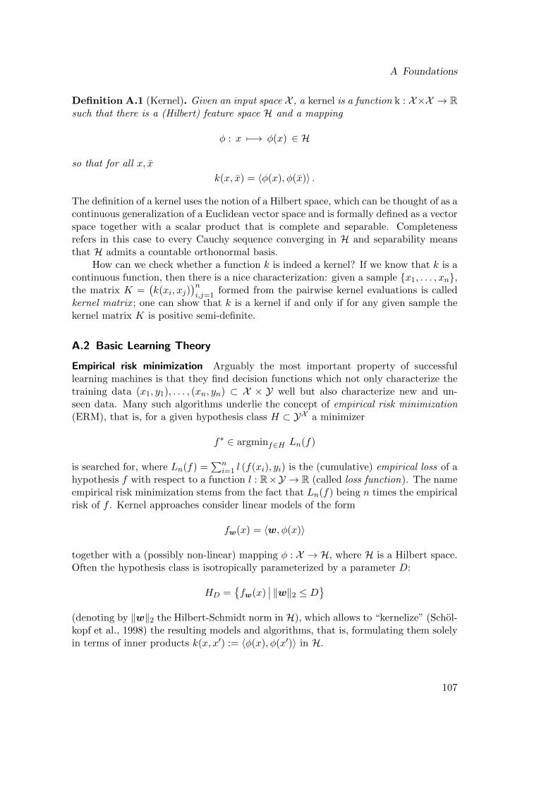
A Foundations
Definition A.1 (Kernel). Given an input space X , a kernel is a function k : X×X → Rsuch that there is a (Hilbert) feature space H and a mapping
φ : x 7−→ φ(x) ∈ H
so that for all x, x
k(x, x) = 〈φ(x), φ(x)〉 .
The definition of a kernel uses the notion of a Hilbert space, which can be thought of as acontinuous generalization of a Euclidean vector space and is formally defined as a vectorspace together with a scalar product that is complete and separable. Completenessrefers in this case to every Cauchy sequence converging in H and separability meansthat H admits a countable orthonormal basis.
How can we check whether a function k is indeed a kernel? If we know that k is acontinuous function, then there is a nice characterization: given a sample x1, . . . , xn,the matrix K =
(k(xi, xj)
)ni,j=1
formed from the pairwise kernel evaluations is calledkernel matrix ; one can show that k is a kernel if and only if for any given sample thekernel matrix K is positive semi-definite.
A.2 Basic Learning Theory
Empirical risk minimization Arguably the most important property of successfullearning machines is that they find decision functions which not only characterize thetraining data (x1, y1), . . . , (xn, yn) ⊂ X × Y well but also characterize new and un-seen data. Many such algorithms underlie the concept of empirical risk minimization(ERM), that is, for a given hypothesis class H ⊂ YX a minimizer
f∗ ∈ argminf∈H Ln(f)
is searched for, where Ln(f) =∑n
i=1 l (f(xi), yi) is the (cumulative) empirical loss of ahypothesis f with respect to a function l : R×Y → R (called loss function). The nameempirical risk minimization stems from the fact that Ln(f) being n times the empiricalrisk of f . Kernel approaches consider linear models of the form
fw(x) = 〈w, φ(x)〉
together with a (possibly non-linear) mapping φ : X → H, where H is a Hilbert space.Often the hypothesis class is isotropically parameterized by a parameter D:
HD =fw(x)
∣∣ ‖w‖2 ≤ D(denoting by ‖w‖2 the Hilbert-Schmidt norm in H), which allows to “kernelize” (Schol-kopf et al., 1998) the resulting models and algorithms, that is, formulating them solelyin terms of inner products k(x, x′) := 〈φ(x), φ(x′)〉 in H.
107
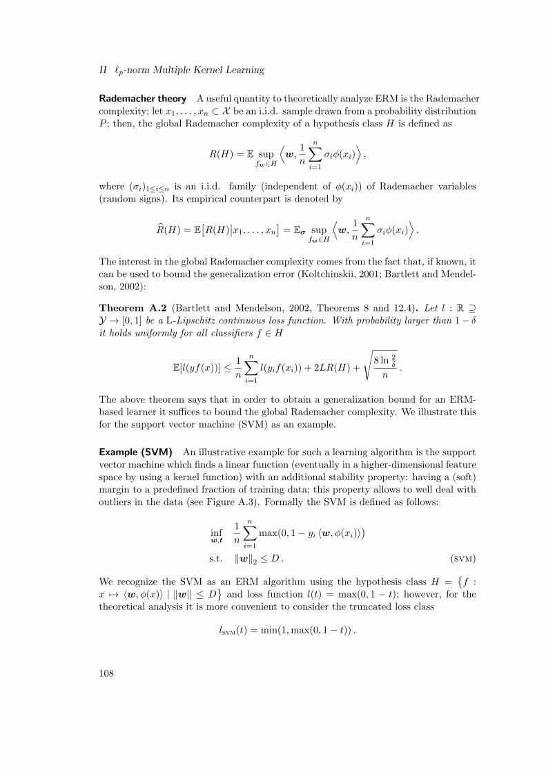
II `p-norm Multiple Kernel Learning
Rademacher theory A useful quantity to theoretically analyze ERM is the Rademachercomplexity; let x1, . . . , xn ⊂ X be an i.i.d. sample drawn from a probability distributionP ; then, the global Rademacher complexity of a hypothesis class H is defined as
R(H) = E supfw∈H
⟨w,
1
n
n∑i=1
σiφ(xi)⟩,
where (σi)1≤i≤n is an i.i.d. family (independent of φ(xi)) of Rademacher variables(random signs). Its empirical counterpart is denoted by
R(H) = E[R(H)
∣∣x1, . . . , xn] = Eσ supfw∈H
⟨w,
1
n
n∑i=1
σiφ(xi)⟩.
The interest in the global Rademacher complexity comes from the fact that, if known, itcan be used to bound the generalization error (Koltchinskii, 2001; Bartlett and Mendel-son, 2002):
Theorem A.2 (Bartlett and Mendelson, 2002, Theorems 8 and 12.4). Let l : R ⊇Y → [0, 1] be a L-Lipschitz continuous loss function. With probability larger than 1− δit holds uniformly for all classifiers f ∈ H
E[l(yf(x))] ≤ 1
n
n∑i=1
l(yif(xi)) + 2LR(H) +
√8 ln 2
δ
n.
The above theorem says that in order to obtain a generalization bound for an ERM-based learner it suffices to bound the global Rademacher complexity. We illustrate thisfor the support vector machine (SVM) as an example.
Example (SVM) An illustrative example for such a learning algorithm is the supportvector machine which finds a linear function (eventually in a higher-dimensional featurespace by using a kernel function) with an additional stability property: having a (soft)margin to a predefined fraction of training data; this property allows to well deal withoutliers in the data (see Figure A.3). Formally the SVM is defined as follows:
infw,t
1
n
n∑i=1
max(0, 1− yi 〈w, φ(xi)〉)
s.t. ‖w‖2 ≤ D . (svm)
We recognize the SVM as an ERM algorithm using the hypothesis class H =f :
x 7→ 〈w, φ(x)〉 | ‖w‖ ≤ D
and loss function l(t) = max(0, 1 − t); however, for thetheoretical analysis it is more convenient to consider the truncated loss class
lsvm(t) = min(1,max(0, 1− t)) .
108
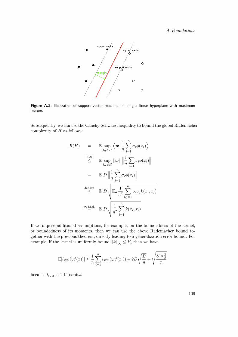
A Foundations
Figure A.3: Illustration of support vector machine: finding a linear hyperplane with maximummargin.
Subsequently, we can use the Cauchy-Schwarz inequality to bound the global Rademachercomplexity of H as follows:
R(H) = E supfw∈H
⟨w,
1
n
n∑i=1
σiφ(xi)⟩
C.-S.≤ E sup
fw∈H‖w‖
∥∥∥ 1
n
n∑i=1
σiφ(xi)∥∥∥
= E D∥∥∥ 1
n
n∑i=1
σiφ(xi)∥∥∥
Jensen≤ E D
√√√√Eσ1
n2
n∑i,j=1
σiσjk(xi, xj)
σi i.i.d.= E D
√√√√ 1
n2
n∑i=1
k(xi, xi)
If we impose additional assumptions, for example, on the boundedness of the kernel,or boundedness of its moments, then we can use the above Rademacher bound to-gether with the previous theorem, directly leading to a generalization error bound. Forexample, if the kernel is uniformly bound ‖k‖∞ ≤ B, then we have
E[lsvm(yf(x))] ≤ 1
n
n∑i=1
lsvm(yif(xi)) + 2D
√B
n+
√8 ln 2
δ
n
because lsvm is 1-Lipschitz.
109
II `p-norm Multiple Kernel Learning
A.3 Convex Optimization
A convex optimization problem (Boyd and Vandenberghe, 2004) is one of the form
minv∈Rn
f(v)
s.t. fi(v) ≤ 0, i = 1, . . . ,m
hi(v) = 0, i = 1, . . . , l, (A.1)
where the functions h1, . . . , hl : Rn 7→ R are affine linear and f0, . . . , fm : Rn 7→ R areconvex, i.e., satisfy fi(αv + βv) ≤ αfi(v) + βfi(v) for all v, v ∈ Rn and all α, β ∈ Rwith α, β = 1, α ≥ 0, and β ≥ 0.
There is no general analytical formula for the solution of such an optimizationproblem, but there are very effective methods for solving them, for example, interior-point methods and limited-memory quasi-Newton methods (Nocedal and Wright, 2006).If we can formulate a problem as a convex optimization problem, then we have solvedthe problem as we can usually solve it efficiently. In contrast, general, non-linearoptimization problems can be very challenging, even with ten variables and intractablewith a few hundreds of variables (Boyd and Vandenberghe, 2004, p. 8–9).
Lagrangian duality An important concept in optimization theory is the Lagrangianduality. The basic idea is to take the constraints in (A.1) into account by augmentingthe objective function with a weighted sum of the constraint functions: we definethe Lagrangian L : Rn × Rm+ × Rl associated with the problem (A.1) as (Boyd andVandenberghe, 2004, p. 215)
L(v,α,β) = f0(v) +m∑i=1
αifi(v) +l∑
i=1
βihi .
We refer to αi as the Lagrangian multiplier associated with the ith inequality constraintand to βi as the Lagrangian multiplier associated with the ith equality constraint. TheLagrangian dual function is defined as the minimum value of the Lagrangian over v:
g(α,β) := infv∈Rn
L(v,α, β) . (A.2)
It is evident that the Lagrangian dual function yields a lower bound for the optimalvalue of the original problem (A.1); to see this, note that violated constraints con-tribute positively in (A.2). It is therefore recommended to maximize the lower bound.This raises the question “what is the best lower bound that can be obtained from theLagrangian dual function?”, leading to the optimization problem
minα,β
g(α,β)
s.t. αi ≥ 0, i = 1, . . . ,m,
110
B Relating Tikhonov and Ivanov Regularization
which is known as the dual problem associated with (A.1). In this context the originalproblem is called primal problem. But how are the optima of the primal and dualproblems related? For convex problems, we have the nice result that both optimalvalues are identical, under rather mild assumptions, which are known as constraintqualifications (CQs). For example, Slater’s condition is such a CQ: there exists a pointv such that hi(v) = 0 and fi(v) < 0 for all i active in the optimum v∗ (Boyd andVandenberghe, 2004, p. 225-226).
B Relating Tikhonov and Ivanov Regularization
In this section, we show a useful result that justifies switching from Tikhonov to Ivanovregularization and vice versa, if the bound on the regularizing constraint is tight. It isa key ingredient of the proof of Theorem 3.1. We state the result for arbitrary convexfunctions, so that it can be applied beyond the multiple kernel learning framework ofthis thesis.
Lemma B.1. Let D ⊂ Rd be a convex set, let f, g : D → R be convex functions.Consider the convex optimization tasks
minv∈D
f(v) + σg(v), (B.1a)
minv∈D:g(v)≤τ
f(v). (B.1b)
Assume that the minima exist and that a constraint qualification holds in (B.1b), whichgives rise to strong duality, e.g., that Slater’s condition is satisfied. Furthermore, as-sume that the constraint is active at the optimal point, i.e.
infv∈D
f(v) < infv∈D:g(v)≤τ
f(v). (B.2)
Then we have the case that for each σ > 0 there exists τ > 0—and vice versa—suchthat the optimization problem (B.1a) is equivalent to (B.1b), i.e., each optimal solutionof one is an optimal solution of the other, and vice versa.
Proof(a). Let be σ > 0 and v∗ be the optimal of (B.1a). We have to show that there existsa τ > 0 such that v∗ is optimal in (B.1b). We set τ = g(v∗). Suppose v∗ is not optimalin (B.1b), i.e., it exists v ∈ D : g(v) ≤ τ such that f(v) < f(v∗). Then we have
f(v) + σg(v) < f(v∗) + στ,
which by τ = g(v∗) translates to
f(v) + σg(v) < f(v∗) + σg(v∗).
This contradicts the optimality of v∗ in (B.1a), and hence proves that v∗ is optimal in(B.1b), which was to be shown.
111
II `p-norm Multiple Kernel Learning
(b). Vice versa, let τ > 0 be v∗ optimal in (B.1b). The Lagrangian of (B.1b) is givenby
L(σ) = f(v) + σ (g(v)− τ) , σ ≥ 0.
By strong duality v∗ is optimal in the saddle point problem
σ∗ := argmaxσ≥0 minv∈D
f(v) + σ (g(v)− τ) ,
and by the strong max-min property (cf. (Boyd and Vandenberghe, 2004), p. 238) wemay exchange the order of maximization and minimization. Hence v∗ is optimal in
minv∈D
f(v) + σ∗ (g(v)− τ) . (B.3)
Removing the constant term −σ∗τ , and setting σ = σ∗, we have that v∗ is optimal in(B.1a), which was to be shown. Moreover by (B.2) we have that
v∗ 6= argminv∈D f(v),
and hence we see from Eq. (B.3) that σ∗ > 0, which completes the proof of the propo-sition.
C Supplements to the Theoretical Analysis
The following result gives a block-structured version of Holder’s inequality (e.g., Steele,2004).
Lemma C.1 (Block-structured Holder inequality). Let v = (v1, . . . ,vM ), w =(w1, . . . ,wM ) ∈ H = H1 × · · · × HM . Then, for any p ≥ 1, it holds
〈v,w〉 ≤ ‖v‖2,p‖w‖2,p∗ .
Proof By the Cauchy-Schwarz inequality (C.-S.), we have for all x,y ∈ H:
〈v,w〉 =M∑m=1
〈vm,wm〉C.-S.≤
M∑m=1
‖vm‖2‖wm‖2
=⟨(‖v1‖2, . . . , ‖vM‖2), (‖w1‖2, . . . , ‖wM‖2)
⟩.
Holder≤ ‖v‖2,p‖w‖2,p∗
Proof of Lemma 4.3 (Rosenthal + Young) It is clear that the result triviallyholds for 1
2 ≤ p ≤ 1 with cq = 1 by Jensen’s inequality . In the case p ≥ 1, we apply
112
C Supplements to the Theoretical Analysis
Rosenthal’s inequality (Rosenthal, 1970) to the sequence X1, . . . , Xn thereby using theoptimal constants computed in Ibragimov and Sharakhmetov (2001), that are, cq = 2(q ≤ 2) and cq = EZq (q ≥ 2), respectively, where Z is a random variable distributedaccording to a Poisson law with parameter λ = 1. This yields
E(
1
n
n∑i=1
Xi
)q≤ cq max
(1
nq
n∑i=1
EXqi ,
(1
n
n∑i=1
Xi
)q). (C.1)
By using the fact that Xi ≤ B holds almost surely, we could readily obtain a bound ofthe form Bq
nq−1 on the first term. However, this is loose and for q = 1 does not convergeto zero when n → ∞. Therefore, we follow a different approach based on Young’sinequality (e.g. Steele, 2004):
1
nq
n∑i=1
EXqi ≤
(B
n
)q−1 1
n
n∑i=1
EXi
Young≤ 1
q∗
(B
n
)q∗(q−1)+
1
q
(1
n
n∑i=1
EXi
)q
=1
q∗
(B
n
)q+
1
q
(1
n
n∑i=1
EXi
)q.
It thus follows from (C.1) that for all q ≥ 12
E(
1
n
n∑i=1
Xi
)q≤ cq
((Bn
)q+( 1
n
n∑i=1
EXi
)q),
where cq can be taken as 2 (q ≤ 2) and EZq (q ≥ 2), respectively, where Z is Poisson-distributed. In the subsequent Lemma C.2 we show EZq ≤ (q + e)q. Clearly, for q ≥ 1
2it holds q + e ≤ qe + eq = 2eq so that in any case cq ≤ max(2, 2eq) ≤ 2eq, whichcompletes the proof.
We use the following Lemma, which gives a handle on the q-th moment of a Poisson-distributed random variable and is used in the previous Lemma.
Lemma C.2. For the q-moment of a random variable Z distributed according to aPoisson law with parameter λ = 1, the following inequality holds for all q ≥ 1:
EZq def.=
1
e
∞∑k=0
kq
k!≤ (q + e)q.
113
II `p-norm Multiple Kernel Learning
Proof We start by decomposing EZq as follows:
Eq =1
e
0 +
q∑k=1
kq
k!+
∞∑k=q+1
kq
k!
=
1
e
q∑k=1
kq−1
(k − 1)!+
∞∑k=q+1
kq
k!
≤ 1
e
qq +∞∑
k=q+1
kq
k!
(C.2)
(C.3)
Note that by Stirling’s approximation it holds k! =√
2πeτkk(ke
)qwith 1
12k+1 < τk <1
12kfor all q. Thus
∞∑k=q+1
kq
k!=
∞∑k=q+1
1√2πeτkk
ekk−(k−q)
=
∞∑k=1
1√2πeτk+q(k + q)
ek+qk−k
= eq∞∑k=1
1√2πeτk+q(k + q)
( ek
)k(∗)≤ eq
∞∑k=1
1√2πeτkk
( ek
)kStirling
= eq∞∑k=1
1
k!
= eq+1
where for (∗) note that eτkk ≤ eτk+q(k + q) can be shown by some algebra using1
12k+1 < τk <1
12k . Now by (C.2)
EZq =1
e
(qq + eq+1
)≤ qq + eq ≤ (q + e)q,
which was to show.
Lemma C.3. For any a, b ∈ Rm+ it holds for all q ≥ 1
‖a‖q + ‖b‖q ≤ 21− 1
q ‖a+ b‖q ≤ 2 ‖a+ b‖q .
114
D Cutting Plane Algorithm
Proof Let a = (a1, . . . , am) and b = (b1, . . . , bm). Because all components of a, b arenonnegative, we have
∀i = 1, . . . ,m : aqi + bqi ≤(ai + bi
)qand thus
‖a‖qq + ‖b‖qq ≤ ‖a+ b‖qq . (C.4)
We conclude by `q-to-`1 conversion (see (4.15))
‖a‖q + ‖b‖q =∥∥( ‖a‖q , ‖b‖q )∥∥1 (4.15)
≤ 21− 1
q∥∥( ‖a‖q , ‖b‖q )∥∥q
= 21− 1
q(‖a‖qq + ‖b‖qq
) 1q
(C.4)
≤ 21− 1
q ‖a+ b‖q ,
which completes the proof.
D Cutting Plane Algorithm
In this section, we present an alternative optimization strategy for the case p ∈ [1, 2],based on the cutting plane method; to this end, we denote q = p/(2 − p) (note thatthus q ∈ [1,∞] since p ∈ [1, 2]). Our algorithm is based on the MKL optimizationproblem II.4. We focus on the hinge loss, i.e., l(t, y) = max(0, 1− ty). Thus, employinga variable substitution of the form αnew
i = αiyi, Problem II.4 translates into
minθ
maxα
1>α− 1
2α>
M∑m=1
θmQmα
s.t. 0 ≤ α ≤ C1; y>α = 0; θ ≥ 0; ‖θ‖qq ≤ 1,
where Qj = Y KjY for 1 ≤ j ≤ m and Y = diag(y). The above optimization problem isa saddle point problem and, as we have seen, can be solved by a block coordinate descentalgorithm, using an analytical formula. We take a different approach and translate themin-max problem into an equivalent semi-infinite program (SIP) as follows. Denotethe value of the target function by t(α,θ) and suppose α∗ is optimal. Then, accordingto the max-min inequality (Boyd and Vandenberghe, 2004, p. 115), we have t(α∗,θ) ≥t(α,θ) for all α and θ. Hence, we can equivalently minimize an upper bound η on theoptimal value and arrive at the following semi-infinite program:
minη
η
s.t. ∀α ∈ A : η ≥ 1>α− 1
2α>
M∑m=1
θmQmα; (SIP)
θ ≥ 0; ‖θ‖qq ≤ 1,
115
II `p-norm Multiple Kernel Learning
Algorithm D.1 (Chunking CPM) Chunking-based `p-Norm MKL cutting plane trainingalgorithm. It simultaneously optimizes the variables α and the kernel weighting θ. The accuracyparameter ε and the subproblem size Q are assumed to be given to the algorithm. For simplicity,a few speed-up tricks are not shown, e.g., hot-starts of the SVM and the QCQP solver.
1: gm,i = 0, gi = 0, αi = 0, η = −∞, θm = q√
1/M for m = 1, . . . ,M and i = 1, . . . , n
2: for t = 1, 2, . . . and while SVM and MKL optimality conditions are not satisfied do3: Select Q suboptimal variables αi1 , . . . , αiQ based on the gradient g and α; store αold = α
4: Solve SVM dual with respect to the selected variables and update α
5: Update gradient gm,i ← gm,i +∑Ql=1(αil − αoldil )yilkm(xil , xi) for all m = 1, . . . ,M and
i = 1, . . . , n
6: for m = 1, . . . ,M do7: Stm = 1
2
∑i gm,iαiyi
8: end for9: Lt =
∑i αi, St =
∑m θmS
tm
10: if |1− Lt−St
η | ≥ ε11: while MKL optimality conditions are not satisfied do12: θold = θ13: (θ, η)← argmin η14: w.r.t. θ ∈ RM , η ∈ R15: s.t. 0 ≤ θ ≤ 1,
16:q(q−1)
2
∑m(θoldm )q−2 θ2m −
∑m q(q − 2)(θoldm )q−1 θm ≤ q(3−q)
2 and17: Lr −
∑m θmS
rm ≤ η for r = 1, . . . , t
18: θ ← θ/||θ||qq19: Remove inactive constraints20: end while21: end if22: gi =
∑m θmgm,i for all i = 1, . . . , n
23: end for
where A =α ∈ Rn | 0 ≤ α ≤ C1,y>α = 0
.
Sonnenburg et al. (2006a) optimize the above SIP for p = 1 with interleavingcutting plane algorithms. The solution of a quadratic program (here the regular SVM)generates the most strongly violated constraint for the actual mixture θ. The optimal(θ∗, η) is then identified by solving a linear program with respect to the set of activeconstraints. The optimal mixture is then used for computing a new constraint and soon.
Unfortunately, for q > 1, a non-linearity is introduced by requiring ‖θ‖qq ≤ 1 andsuch constraint is unlikely to be found in standard optimization toolboxes that oftenhandle only linear and quadratic constraints. As a remedy, we propose to approximate
116
D Cutting Plane Algorithm
the constraint ‖θ‖qq ≤ 1 by a sequence of second-order Taylor expansions9
||θ||qq ≈ ||θ||qq + q(θq−1)> (
θ − θ)
+q(q − 1)
2
(θ − θ
)>diag
(θq−2)(
θ − θ)
= 1 +q(q − 3)
2−
M∑m=1
q(q − 2)(θm)q−1 θm +q(q − 1)
2
M∑m=1
θq−2m θ2m,
where θq is defined element-wise, that is θq := (θq1, . . . , θqM ). The sequence (θ0,θ1, · · · )
is initialized with a uniform mixture satisfying ||θ0||qq = 1 as a starting point. Succes-sively, θt+1 is computed using θ = θt. Note that the Hessian of the quadratic termin the approximation is diagonal, strictly positive and very-well conditioned, for whichreason the resulting quadratically constrained problem can be solved efficiently. Infact, since there is only one quadratic constraint, its complexity should rather be com-pared to that of a considerably easier quadratic program. Moreover, in order to ensureconvergence, we enhance the resulting sequential quadratically constrained quadraticprogramming by projection steps onto the boundary of the feasible set, as given inLine 18. Finally, note that this approach can be further sped-up by additional level-setprojections in the θ-optimization phase similar to Xu et al. (2009). In our case, thelevel-set projection is a convex quadratic problem with `p-norm constraints and canagain be approximated by a successive sequence of second-order Taylor expansions.
Algorithm D.1 outlines the interleaved α,θ MKL training algorithm. Lines 3-5are standard in chunking based SVM solvers and carried out by SVMlight. Lines 6-9compute (parts of) SVM objective values for each kernel independently. Finally lines11 to 19 solve a sequence of semi-infinite programs with the `p-norm constraint beingapproximated as a sequence of second-order constraints. The algorithm terminates ifthe maximal KKT violation (see Joachims, 1999) falls below a predetermined precisionεsvm and if the normalized maximal constraint violation |1− L−St
η | < εmkl for the MKL.The following proposition shows the convergence of the semi-infinite programming loopin Algorithm D.1.
Proposition D.1. Let the kernel matrices K1, . . . ,KM be positive-definite and be q >1. Suppose that the SVM computation is solved exactly in each iteration. Moreover,suppose there exists an optimal limit point of nested sequence of QCCPs. Then thesequence generated by Algorithm D.1 has at least one point of accumulation that solves(P).
Proof By assumption, the SVM is solved to infinite precision in each MKL step,which simplifies our analysis in that the numerical details in Algorithm D.1 can beignored. We conclude that the outer loop of Alg. D.1 amounts to a cutting-plane algo-rithm for solving the semi-infinite program of Optimization Problem (SIP). It is well
9We also tried out first-order Taylor expansions, whereby our algorithm basically boils down therenowned sequential quadratic programming, but, empirically, it turned out to be inferior. Intu-itively, second-order expansions work best when the approximated function is almost quadratic, asgiven in our case.
117
II `p-norm Multiple Kernel Learning
known (Sonnenburg et al., 2006a) that this algorithm converges, in the sense that thereexists at least one point of accumulation that solves the primal problem (P). E.g.,this can be seen by viewing the cutting plane algorithm as a special instance of theclass of so-called exchange methods and subsequently applying Theorem 7.2 in Hettichand Kortanek (1993). A difference to the analysis in Sonnenburg et al. (2006a) is the`p>1-norm constraint in our algorithm. However, according to our assumption that thenonlinear subprogram is solved correctly, a quick inspection of the preliminaries of thelatter theorem clearly reveals, that they remain fulfilled when introducing an `p-normconstraint.
In order to complete our convergence analysis, it remains to show that the inner loop(lines 11-18), that is, the sequence of QCQPs, converges against an optimal point.Existing analyses of this so-called sequential quadratically constrained quadratic pro-gramming (SQCQP) can be divided into two classes. First, one class establishes localconvergence, i.e., convergence in an open neighborhood of the optimal point, at a rateof O(n2), under relatively mild smoothness and constraint qualification assumptions(Fernandez and Solodov, 2008; Anitescu, 2002), whereas Anitescu (2002) addition-ally requires quadratic growth of the nonlinear constraints. Those analyses basicallyguarantee local convergence the nested sequences of QCQPs in our `q-norm trainingalgorithm, for all q ∈ (1,∞) (Fernandez and Solodov, 2008) and q ≥ 2 (Anitescu, 2002),respectively.
A second class of papers additionally establishes global convergence (e.g. Solodov,2004; Fukushima et al., 2002), so they need more restrictive assumptions. Moreover,in order to ensure feasibility of the subproblems when the actual iterate is too faraway from the true solution, a modification of the algorithmic protocol is needed. Thisis usually dealt with by performing a subsequent line search and downweighting thequadratic term by a multiplicative adaptive constant Di ∈ [0, 1]. Unfortunately, thelatter involves a complicated procedure to tune Di (Fukushima et al., 2002, p. 7).Employing the above modifications, the analysis in Fukushima et al. (2002) togetherwith our Prop. D.1 would guarantee the convergence of our Alg. D.1.
However, due to the special form of our SQCQP, we chose to discard the com-fortable convergence guarantees and to proceed with a much more simple and efficientstrategy, which renders both the expensive line search and the tuning of the constantDi unnecessary. The idea of our method is that the projection of θ onto the boundaryof the feasible set, given by line 18 in Alg. D.1, can be performed analytically. Thisprojection ensures the feasibility of the QCQP subproblems. Note that in general, thisprojection can be as expensive as performing a QCQP step, which is why, to the best ofour knowledge, projection-type algorithms for solving SQCQPs have not been studiedyet by the optimization literature.
Although the projection procedure is appealingly simple and—as we found outempirically—seemingly shares nice convergence properties (the sequence of SQCQPsconverged optimally in all cases we tried, usually after 3-4 iterations), it unfortunatelyprohibits exploitation of existing analyses for global convergence. However, the discus-
118

D Cutting Plane Algorithm
sions in Fukushima et al. (2002) and Solodov (2004) identify the reason of occasionaldivergence of the vanilla SQCQP as the infeasibility of the subproblems. But in con-trast, our projection algorithm always ensures the feasibility of the subproblem. Wetherefore conjecture that, based on the superior empirical results and the discussions inFukushima et al. (2002) and Solodov (2004), our algorithm is designated to converge.The theoretical analysis of this new class of SQCQP projection algorithms is beyondthe scope of this thesis.
119

Bibliography
T. Abeel, Y. V. de Peer, and Y. Saeys. Towards a gold standard for promoter predictionevaluation. Bioinformatics, 2009.
J. Aflalo, A. Ben-Tal, C. Bhattacharyya, J. S. Nath, and S. Raman. Variable sparsity kernellearning—algorithms and applications. Journal of Machine Learning Research, 12:565–592,Feb 2011.
B. Alberts, A. Johnson, J. Lewis, M. Raff, K. Roberts, and P. Walter. Molecular biology of thecell. Garland Science, 4 edition, 2002. ISBN 0815332181.
M. Anitescu. A superlinearly convergent sequential quadratically constrained quadratic pro-gramming algorithm for degenerate nonlinear programming. SIAM J. on Optimization, 12(4):949–978, 2002.
F. Bach. Eccv 2008 tutorial on supervised learning, 2008a.
F. R. Bach. Consistency of the group lasso and multiple kernel learning. J. Mach. Learn. Res.,9:1179–1225, 2008b.
F. R. Bach, G. R. G. Lanckriet, and M. I. Jordan. Multiple kernel learning, conic duality, andthe SMO algorithm. In Proc. 21st ICML. ACM, 2004.
V. B. Bajic, S. L. Tan, Y. Suzuki, and S. Sugano. Promoter prediction analysis on the wholehuman genome. Nature Biotechnology, 22(11):1467–1473, 2004.
P. Bartlett and S. Mendelson. Rademacher and gaussian complexities: Risk bounds and struc-tural results. Journal of Machine Learning Research, 3:463–482, Nov. 2002.
P. L. Bartlett and S. Mendelson. Empirical minimization. Probability Theory and RelatedFields, 135(3):311–334, 2006.
P. L. Bartlett, O. Bousquet, and S. Mendelson. Local Rademacher complexities. Annals ofStatistics, 33(4):1497–1537, 2005.
D. Bertsekas. Nonlinear Programming, Second Edition. Athena Scientific, Belmont, MA, 1999.
A. Binder, K.-R. Muller, and M. Kawanabe. On taxonomies for multi-class image categorization.International Journal of Computer Vision, January 2011.
K. Bleakley, G. Biau, and J.-P. Vert. Supervised reconstruction of biological networks withlocal models. Bioinformatics, 23:i57–i65, 2007.
A. Bosch, A. Zisserman, and X. Munoz. Representing shape with a spatial pyramid kernel. InProceedings of the 6th ACM international conference on Image and video retrieval (CIVR’07), pages 401–408, 2007. ISBN 978-1-59593-733-9.
121
Bibliography
O. Bousquet, S. Boucheron, and G. Lugosi. Introduction to statistical learning theory. InO. Bousquet, U. von Luxburg, and G. Ratsch, editors, Advanced Lectures on Machine Learn-ing, volume 3176 of Lecture Notes in Computer Science, pages 169–207. Springer Berlin /Heidelberg, 2004.
S. Boyd and L. Vandenberghe. Convex Optimization. Cambrigde University Press, Cambridge,UK, 2004.
C. Campbell and Y. Ying. Learning with Support Vector Machines. Synthesis Lectures onArtificial Intelligence and Machine Learning. Morgan & Claypool Publishers, 2011.
J. Canny. A computational approach to edge detection. IEEE Trans. on Pattern Analysis andMachine Intelligence, 8:679–714, 1986.
O. Chapelle and A. Rakotomamonjy. Second order optimization of kernel parameters. In Proc.of the NIPS Workshop on Kernel Learning: Automatic Selection of Optimal Kernels, 2008.
O. Chapelle, B. Scholkopf, and A. Zien, editors. Semi-Supervised Learning. MIT Press, Cam-bridge, MA, 2006. URL http://www.kyb.tuebingen.mpg.de/ssl-book.
C. Cortes. Invited talk: Can learning kernels help performance? In Proceedings of the 26th An-nual International Conference on Machine Learning, ICML ’09, pages 1:1–1:1, New York, NY,USA, 2009. ACM. ISBN 978-1-60558-516-1. Video http://videolectures.net/icml09_
cortes_clkh/.
C. Cortes, A. Gretton, G. Lanckriet, M. Mohri, A. Rostamizadeh, and editors, editors. Proceed-ings of the NIPS 2008 workshop on kernel learning: automatic selection of optimal kernels,2008. URL http://www.cs.nyu.edu/learning_kernels, Video http://videolectures.
net/lkasok08_whistler/.
C. Cortes, M. Mohri, and A. Rostamizadeh. L2 regularization for learning kernels. In Proceed-ings of the International Conference on Uncertainty in Artificial Intelligence, 2009a.
C. Cortes, M. Mohri, and A. Rostamizadeh. Learning non-linear combinations of kernels. InY. Bengio, D. Schuurmans, J. Lafferty, C. K. I. Williams, and A. Culotta, editors, Advancesin Neural Information Processing Systems 22, pages 396–404, 2009b.
C. Cortes, M. Mohri, and A. Rostamizadeh. Generalization bounds for learning kernels. InProceedings, 27th ICML, 2010a.
C. Cortes, M. Mohri, and A. Rostamizadeh. Two-stage learning kernel algorithms. In Proceed-ings of the 27th Conference on Machine Learning (ICML 2010), 2010b.
N. Cristianini, J. Shawe-Taylor, A. Elisseeff, and J. Kandola. On kernel-target alignment. InT. Fawcett and N. Mishra, editors, Advances in Neural Information Processing Systems,volume 14, pages 367–373, 2002.
G. Csurka, C. Bray, C. Dance, and L. Fan. Visual categorization with bags of keypoints. InWorkshop on Statistical Learning in Computer Vision, ECCV, volume 2, pages 1–22, Prague,Czech Republic, May 2004.
N. Dalal and B. Triggs. Histograms of oriented gradientsfor human detection. In IEEE Com-puter Society Conference on Computer Vision and Pattern Recognition, volume 1, pages886–893, San Diego, USA, June 2005.
122
Bibliography
M. Everingham, L. Van Gool, C. K. I. Williams, J. Winn, and A. Zisserman. The PAS-CAL Visual Object Classes Challenge 2008 (VOC2008) Results, 2008. URL http://www.
pascal-network.org/challenges/VOC/voc2008/workshop/index.html.
T. Evgeniou and M. Pontil. Regularized multi–task learning. In W. Kim, R. Kohavi, J. Gehrke,and W. DuMouchel, editors, KDD, pages 109–117. ACM, 2004. ISBN 1-58113-888-1.
R. Fan, K. Chang, C. Hsieh, X. Wang, and C. Lin. LIBLINEAR: A library for large linearclassification. Journal of Machine Learning Research, 9:1871–1874, 2008.
D. Fernandez and M. Solodov. On local convergence of sequential quadratically-constrainedquadratic-programming type methods, with an extension to variational problems. Comput.Optim. Appl., 39(2):143–160, 2008.
V. Franc and S. Sonnenburg. OCAS optimized cutting plane algorithm for support vectormachines. In Proceedings of the 25nd International Machine Learning Conference. ACMPress, 2008.
M. Fukushima, Z.-Q. Luo, and P. Tseng. A sequential quadratically constrained quadraticprogramming method for differentiable convex minimization. SIAM J. on Optimization, 13(4):1098–1119, 2002.
P. Gehler and S. Nowozin. Infinite kernel learning. In Proceedings of the NIPS 2008 Workshopon Kernel Learning: Automatic Selection of Optimal Kernels, 2008.
P. V. Gehler and S. Nowozin. On feature combination for multiclass object classification. InICCV, pages 221–228, 2009.
G. Golub and C. van Loan. Matrix Computations. John Hopkins University Press, Baltimore,London, 3rd edition, 1996.
N. Gornitz, M. Kloft, and U. Brefeld. Active and semi-supervised data domain description.In W. L. Buntine, M. Grobelnik, D. Mladenic, and J. Shawe-Taylor, editors, Proceedingsof the European Conference on Machine Learning and Knowledge Discovery in Databases(ECML/PKDD), pages 407–422, 2009a.
N. Gornitz, M. Kloft, K. Rieck, and U. Brefeld. Active learning for network intrusion detection.In Proc. of CCS Workshop on Security and Artificial Intelligence (AISEC), pages 47–54, NewYork, NY, USA, 2009b. ACM.
N. Gornitz, M. Kloft, K. Rieck, and U. Brefeld. Active and semi-supervised domain descriptionsin theory and practice. Journal of Artificial Intelligence Research (JAIR), 2010. submitted07/2010.
R. Hettich and K. O. Kortanek. Semi-infinite programming: theory, methods, and applications.SIAM Rev., 35(3):380–429, 1993.
R. Ibragimov and S. Sharakhmetov. The best constant in the rosenthal inequality for non-negative random variables. Statistics & Probability Letters, 55(4):367 – 376, 2001. ISSN0167-7152.
R. Jenssen, M. Kloft, A. Zien, S. Sonnenburg, and K.-R. Muller. A multi-class support vectormachine based on scatter criteria. Technical Report 014-2009, Technische Universitat Berlin,Jul 2009. Revised version submitted to Pattern Recognition, Apr 2011.
123
Bibliography
T. Joachims. Making large–scale SVM learning practical. In B. Scholkopf, C. Burges, andA. Smola, editors, Advances in Kernel Methods — Support Vector Learning, pages 169–184,Cambridge, MA, 1999. MIT Press.
J.-P. Kahane. Some random series of functions. Cambridge University Press, 2nd edition, 1985.
M. Kanehisa, S. Goto, S. Kawashima, Y. Okuno, and M. Hattori. The KEGG resource fordeciphering the genome. Nucleic Acids Res, 32:D277–D280, 2004.
G. Kimeldorf and G. Wahba. Some results on tchebycheffian spline functions. J. Math. Anal. Ap-plic., 33:82–95, 1971.
M. Kloft and G. Blanchard. The local rademacher complexity of lp-norm multiple kernellearning. Technical report, Arxiv preprint 1103.0790v1, Mar 2011. URL http://arxiv.org/
abs/1103.0790v1. Full version submitted to Journal of Machine Learning Research, Mar2011. Short Version submitted to Twenty-Fifth Annual Conference on Neural InformationProcessing Systems (NIPS 2011).
M. Kloft and P. Laskov. Online anomaly detection under adversarial impact. In Y. W. Tehand M. Titterington, editors, JMLR Workshop and Conference Proceedings, Volume 9: AIS-TATS, pages 405–412. MIT Press, 2010a.
M. Kloft and P. Laskov. Security analysis of online centroid anomaly detection. Technical Re-port UCB/EECS-2010-22, EECS Department, University of California, Berkeley, Feb 2010b.URL http://www.eecs.berkeley.edu/Pubs/TechRpts/2010/EECS-2010-22.html. CoRRabs/1003.0078. Revised version submitted to Journal of Machine Learning Resarch, Feb 2011.
M. Kloft, U. Brefeld, P. Dussel, C. Gehl, and P. Laskov. Automatic feature selection for anomalydetection. In D. Balfanz and J. Staddon, editors, AISec, pages 71–76. ACM, 2008a.
M. Kloft, U. Brefeld, P. Laskov, and S. Sonnenburg. Non-sparse multiple kernel learning. InProc. of the NIPS Workshop on Kernel Learning: Automatic Selection of Kernels, Dec 2008b.URL http://www.cs.nyu.edu/learning_kernels/abstracts/ws_mkl.pdf.
M. Kloft, U. Brefeld, S. Sonnenburg, P. Laskov, K.-R. Muller, and A. Zien. Efficient andaccurate lp-norm multiple kernel learning. In Y. Bengio, D. Schuurmans, J. Lafferty, C. K. I.Williams, and A. Culotta, editors, Advances in Neural Information Processing Systems 22,pages 997–1005. MIT Press, 2009a.
M. Kloft, S. Nakajima, and U. Brefeld. Feature selection for density level-sets. In W. L. Bun-tine, M. Grobelnik, D. Mladenic, and J. Shawe-Taylor, editors, Proceedings of the EuropeanConference on Machine Learning and Knowledge Discovery in Databases (ECML/PKDD),pages 692–704, 2009b.
M. Kloft, U. Ruckert, and P. L. Bartlett. A unifying view of multiple kernel learning. InProceedings of the European Conference on Machine Learning and Knowledge Discovery inDatabases (ECML/PKDD), pages 66–81, 2010a.
M. Kloft, U. Ruckert, C. S. Ong, A. Rakotomamonjy, S. Sonnenburg, and F. Bach, editors.Proceedings of the NIPS 2010 workshop on new directions in multiple kernel learning, 2010b.URL http://doc.ml.tu-berlin.de/mkl_workshop/, Video http://videolectures.net/
nipsworkshops2010_kernel_learning/.
124
Bibliography
M. Kloft, U. Brefeld, S. Sonnenburg, and A. Zien. Lp-norm multiple kernel learning. Journalof Machine Learning Research, 12:953–997, Mar 2011.
V. Koltchinskii. Rademacher penalties and structural risk minimization. IEEE Transactionson Information Theory, 47(5):1902–1914, 2001.
V. Koltchinskii. Local Rademacher complexities and oracle inequalities in risk minimization.Annals of Statistics, 34(6):2593–2656, 2006.
V. Koltchinskii. Sparsity in penalized empirical risk minimization. Annales de l’Institut HenriPoincare, Probabilites et Statistiques, 45(1):7–57, 2009.
V. Koltchinskii and D. Panchenko. Empirical margin distributions and bounding the general-ization error of combined classifiers. Annals of Statistics, 30:1–50, 2002.
V. Koltchinskii and M. Yuan. Sparsity in multiple kernel learning. Annals of Statistics, 38(6):3660–3695, 2010.
S. Kwapien and W. A. Woyczynski. Random Series and Stochastic Integrals: Single and Mul-tiple. Birkhauser, Basel and Boston, M.A., 1992.
C. Lampert and M. Blaschko. A multiple kernel learning approach to joint multi-class objectdetection. In DAGM, pages 31–40, 2008.
G. Lanckriet, N. Cristianini, L. E. Ghaoui, P. Bartlett, and M. I. Jordan. Learning the kernelmatrix with semi-definite programming. JMLR, 5:27–72, 2004a.
G. Lanckriet, F. Bach, N. Srebro, and B. McFee, editors. Proceedings of the NIPS 2009 Work-shop on Understanding Multiple Kernel Learning Methods, 2009. URL http://mkl.ucsd.
edu/workshop.
G. R. G. Lanckriet, T. De Bie, N. Cristianini, M. I. Jordan, and W. S. Noble. A statisticalframework for genomic data fusion. Bioinformatics, 20:2626–2635, November 2004b. ISSN1367-4803.
P. Laskov and M. Kloft. A framework for quantitative security analysis of machine learning. InD. Balfanz and J. Staddon, editors, Proceedings of the 2nd ACM Workshop on Security andArtificial Intelligence (AISEC), pages 1–4, 2009.
S. Lazebnik, C. Schmid, and J. Ponce. Beyond bags of features: Spatial pyramid matchingfor recognizing natural scene categories. In Proceedings of the 2006 IEEE Computer SocietyConference on Computer Vision and Pattern Recognition (CVPR ’06), volume 2, pages 2169–2178, New York, USA, 2006.
D. Liu and J. Nocedal. On the limited memory method for large scale optimization. Mathe-matical Programming B, 45(3):503–528, 1989.
D. G. Lowe. Distinctive image features from scale-invariant keypoints. International Journalof Computer Vision, 60(2):91–110, 2004.
M. Markou and S. Singh. Novelty detection: a review – part 1: statistical approaches. SignalProcessing, 83:2481–2497, 2003a.
125
Bibliography
M. Markou and S. Singh. Novelty detection: a review – part 2: neural network based approaches.Signal Processing, 83:2499–2521, 2003b.
M. Marszalek and C. Schmid. Learning representations for visual object class recognition. InProceedings of the PASCAL Visual Object Classes Challenge 2007 (VOC2007), 2007.
A. F. Martins, M. A. Figueiredo, P. M. Aguiar, N. A. Smith, and E. P. Xing. Online learning ofstructured predictors with multiple kernels. In JMLR Workshop and Conference Proceedings:AISTATS 2011. MIT Press, 2011. To appear.
S. Mendelson. On the performance of kernel classes. J. Mach. Learn. Res., 4:759–771, December2003.
K.-R. Muller, S. Mika, G. Ratsch, K. Tsuda, and B. Scholkopf. An introduction to kernel-basedlearning algorithms. IEEE Neural Networks, 12(2):181–201, May 2001.
S. Nakajima, A. Binder, C. Muller, W. Wojcikiewicz, M. Kloft, U. Brefeld, K.-R. Muller, andM. Kawanabe. Multiple kernel learning for object classification. In Proceedings of the 12thWorkshop on Information-based Induction Sciences, 2009a.
S. Nakajima, A. Binder, C. Muller, W. Wojcikiewicz, M. Kloft, U. Brefeld, K.-R. Muller, andM. Kawanabe. Multiple kernel learning for object classification. In Proceedings of the 12thWorkshop on Information-based Induction Sciences, 2009b.
S. Nakajima, A. Binder, C. Muller, W. Wojcikiewicz, M. Kloft, U. Brefeld, K.-R. Muller, andM. Kawanabe. Multiple kernel learning for object classification. IEEE Transactions onPattern Analysis and Machine Intelligence (TPAMI), 2010. submitted 09/2010.
W. S. Noble. Multi-kernel learning for biology. In Proceedings of the NIPS Workshop on KernelLearning: Automatic Selection of Optimal Kernels, 2008. URL http://videolectures.net/
lkasok08_noble_mklfb/.
J. Nocedal and S. J. Wright. Numerical Optimization. Springer, New York, 2nd edition, 2006.
G. Obozinski, M. J. Wainwright, and M. I. Jordan. Support union recovery in high-dimensionalmultivariate regression. Ann. Stat., 39(1):1–47, 2011.
C. S. Ong and A. Zien. An Automated Combination of Kernels for Predicting Protein Subcel-lular Localization. In Proc. of the 8th Workshop on Algorithms in Bioinformatics, 2008.
C. S. Ong, A. J. Smola, and R. C. Williamson. Learning the kernel with hyperkernels. Journalof Machine Learning Research, 6:1043–1071, 2005.
F. Orabona and L. Jie. Ultra-fast optimization algorithm for sparse multi kernel learning. InProceedings of the 28th Annual International Conference on Machine Learning, ICML ’11,2011. To appear.
F. Orabona, J. Luo, and B. Caputo. Online-batch strongly convex multi kernel learning. InCVPR, pages 787–794. IEEE, 2010.
A. Rakotomamonjy, F. Bach, S. Canu, and Y. Grandvalet. SimpleMKL. Journal of MachineLearning Research, 9:2491–2521, 2008.
126
Bibliography
G. Raskutti, M. J. Wainwright, and B. Yu. Minimax-optimal rates for sparse additive modelsover kernel classes via convex programming. CoRR, abs/1008.3654, 2010.
R. M. Rifkin and R. A. Lippert. Value regularization and Fenchel duality. J. Mach. Learn.Res., 8:441–479, 2007.
H. Rosenthal. On the subspaces of Lp (p > 2) spanned by sequences of independent randomvariables. Israel J. Math., 8:273–303, 1970.
V. Roth and B. Fischer. The group-lasso for generalized linear models: uniqueness of solutionsand efficient algorithms. In Proceedings of the Twenty-Fifth International Conference onMachine Learning (ICML 2008), volume 307, pages 848–855. ACM, 2008.
U. Ruckert and M. Kloft. Transfer learning with adaptive regularizers. In Proceedingsof the European Conference on Machine Learning and Knowledge Discovery in Databases(ECML/PKDD), 2011.
B. Scholkopf, A. Smola, and K.-R. Muller. Nonlinear component analysis as a kernel eigenvalueproblem. Neural Computation, 10:1299–1319, 1998.
B. Scholkopf, S. Mika, C. Burges, P. Knirsch, K.-R. Muller, G. Ratsch, and A. Smola. Inputspace vs. feature space in kernel-based methods. IEEE Transactions on Neural Networks, 10(5):1000–1017, September 1999.
B. Scholkopf, J. Platt, J. Shawe-Taylor, A. Smola, and R. Williamson. Estimating the supportof a high-dimensional distribution. Neural Computation, 13(7):1443–1471, 2001.
B. Scholkopf, K. Tsuda, and J. P. Vert, editors. Kernel Methods in Computational Biology.MIT Press, 2004.
J. R. Searle. Minds, brains, and programs. Behavioral and Brain Sciences, 3(03):417–424, 1980.
J. Shawe-Taylor and N. Cristianini. Kernel methods for pattern analysis. Cambridge UniversityPress, 2004.
M. Sion. On general minimax theorems. Pacific J. Math., 8(1):171–176, 1958.
M. V. Solodov. On the sequential quadratically constrained quadratic programming methods.Math. Oper. Res., 29(1):64–79, 2004.
S. Sonnenburg. Machine Learning for Genomic Sequence Analysis. PhD thesis, FraunhoferInstitute FIRST, December 2008.
S. Sonnenburg, G. Ratsch, C. Schafer, and B. Scholkopf. Large scale multiple kernel learning.Journal of Machine Learning Research, 7:1531–1565, July 2006a.
S. Sonnenburg, A. Zien, and G. Ratsch. Arts: Accurate recognition of transcription starts inhuman. Bioinformatics, 22(14):e472–e480, 2006b.
S. Sonnenburg, G. Ratsch, S. Henschel, C. Widmer, J. Behr, A. Zien, F. de Bona, A. Binder,C. Gehl, and V. Franc. The SHOGUN Machine Learning Toolbox. Journal of MachineLearning Research, 2010.
127
Bibliography
J. M. Steele. The Cauchy-Schwarz Master Class: An Introduction to the Art of MathematicalInequalities. Cambridge University Press, New York, NY, USA, 2004. ISBN 052154677X.
Y. Suzuki, R. Yamashita, K. Nakai, and S. Sugano. dbTSS: Database of human transcriptionalstart sites and full-length cDNAs. Nucleic Acids Research, 30(1):328–331, 2002.
M. Szafranski, Y. Grandvalet, and A. Rakotomamonjy. Composite kernel learning. Mach.Learn., 79(1-2):73–103, 2010.
A. Tsybakov. Optimal rates of aggregation. In B. Scholkopf and M. Warmuth, editors, Compu-tational Learning Theory and Kernel Machines (COLT-2003), volume 2777 of Lecture Notesin Artificial Intelligence, pages 303–313. Springer, 2003.
V. N. Vapnik. Statistical Learning Theory. Wiley-Interscience, Sept. 1998.
M. Varma and B. R. Babu. More generality in efficient multiple kernel learning. In Proceedingsof the 26th Annual International Conference on Machine Learning (ICML), pages 1065–1072,New York, NY, USA, 2009. ACM.
M. Varma and D. Ray. Learning the discriminative power-invariance trade-off. In IEEE 11thInternational Conference on Computer Vision (ICCV), pages 1–8, 2007.
U. von Luxburg. A tutorial on spectral clustering. Statistics and Computing, 17(4):395–416,2007.
C. Widmer, N. Toussaint, Y. Altun, and G. Ratsch. Inferring latent task structure for multitasklearning by multiple kernel learning. BMC Bioinformatics, 11(Suppl 8):S5, 2010.
R. C. Williamson, A. J. Smola, and B. Scholkopf. Generalization performance of regularizationnetworks and support vector machines via entropy numbers of compact operators. IEEETransactions on Information Theory, 47(6):2516–2532, 2001.
Z. Xu, R. Jin, I. King, and M. Lyu. An extended level method for efficient multiple kernellearning. In D. Koller, D. Schuurmans, Y. Bengio, and L. Bottou, editors, Advances inNeural Information Processing Systems 21, pages 1825–1832, 2009.
Y. Yamanishi, , J.-P. Vert, and M. Kanehisa. Supervised enzyme network inference from theintegration of genomic data and chemical information. Bioinformatics, 21:i468–i477, 2005.
F. Yan, K. Mikolajczyk, M. Barnard, H. Cai, and J. Kittler. Lp norm multiple kernel fisherdiscriminant analysis for object and image categorisation. In IEEE International Conferenceon Computer Vision and Pattern Recognition, 2010.
S. Yu, T. Falck, A. Daemen, L.-C. Tranchevent, J. Suykens, B. De Moor, and Y. Moreau.L2-norm multiple kernel learning and its application to biomedical data fusion. BMC Bioin-formatics, 11(1):309, 2010. ISSN 1471-2105.
M. Yuan and Y. Lin. Model selection and estimation in regression with grouped variables.Journal of the Royal Statistical Society, Series B, 68:49–67, 2006.
J. Zhang, M. Marszalek, S.Lazebnik, and C. Schmid. Local features and kernels for classificationof texture and object categories: A comprehensive study. International Journal of ComputerVision, 73(2):213–238, 2007.
128

Bibliography
A. Zien and C. S. Ong. Multiclass multiple kernel learning. In Proceedings of the 24th interna-tional conference on Machine learning (ICML), pages 1191–1198. ACM, 2007.
129

Curriculum Vitae
Personal Information
Name Marius KloftDate of birth July 16, 1980Place of birth Dernbach, Rhineland-Palatinate, GermanyCitizenship GermanEmail [email protected]
Education and Employment
since 01/2007 PhD studies in Computer Science at the Machine Learning Laboratory, Depart-ment of EECS, Berlin Institute of Technology (TU Berlin). Advisor: Prof. Dr.Klaus-Robert Muller.
since 10/2010 PhD scholarship by the Berlin Institute of Technology (TU Berlin).
10/2009–09/2010 Research stay at the Learning Theory Group, EECS department, University ofCalifornia, Berkeley, USA. Founded by a scholarship of the German ForeignExchange Service (DAAD). Advisor: Prof. Dr. Peter L. Bartlett.
06/2007–09/2009 Employment in the BMBF project Real-time Machine Learning for IntrusionDetection (REMIND) in collaboration with the Fraunhofer FIRST Institute,Berlin. Supervisor: Pavel Laskov, PhD.
01/2007–04/2007 Employment in the BMBF project FASOR.
07/2006 Diploma in mathematics (M.Sc. equivalent) with GPA 1.0 (1.0 is max).
Diploma thesis in algebraic geometry on Stable Base Loci and the Theorem ofZariski-Fujita. Advisor: Prof. Dr. Thomas Bauer.
10/2001–07/2006 Studies in mathematic with minor computer science at the University of Mar-burg, Germany.
Majors: Algebraic geometry, algebra, complex geometry, probability theory,universal algebra.
10/2000–09/2001 Studies in physics at the University of Marburg, Germany.
09/2000 Internship at Klockner Pentaplast of America, Gordonsville, VA, USA.
07/2000 Award by the German physical society for achievements in the high schoolmajor physics.
08/1989–07/2000 Mons-Tabor Gymnasium Montabaur (high school)
131

Publications
Publications related to this thesis are marked with •, others with .
Preprints (submitted)
D. Deb, J. Lassig, and M. Kloft. Effects of Seedling Age and Land Type on Grain Yield inthe System of Rice Intensification. Submitted to Experimental Agriculture, Jun 2011. [27]
• M. Kloft and G. Blanchard. The Local Rademacher Complexity of `p-Norm Multiple KernelLearning. ArXiv preprint 1103.0790, Mar 2011. Submitted to Journal of Machine LearningResearch (JMLR). Status: Accepted pending minor revision. [26]
R. Jenssen, M. Kloft, A. Zien, S. Sonnenburg, and K.-R. Muller. A Multi-Class SupportVector Machine based on Scatter Criteria. Technical Report 14/2009, Technische UniversitatBerlin, Jun 2009. Submitted to Pattern Recognition. Status: revision. Revision submitted,Apr 2011. [25]
M. Kloft and P. Laskov. Security Analysis of Online Centroid Anomaly Detection. TechnicalReport UCB/EECS-2010-22, University of California, Berkeley, Feb 2010. Submitted to Jour-nal of Machine Learning Research (JMLR). Status: Accepted pending minor revision. [24]
• A. Binder, S. Nakajima, M. Kloft, C. Muller, W. Wojcikiewicz, U. Brefeld, K.-R. Muller,and M. Kawanabe. Classifying Visual Objects with many Kernels. Submitted to Transactionsof Pattern Analysis and Machine Intelligence (TPAMI). Status: major revision. Revision inpreparation. [23]
N. Gornitz, M. Kloft, K. Rieck, and U. Brefeld. From Unsupervised towards SupervisedAnomaly Detection. Submitted to Journal of Artificial Intelligence Research (JAIR). Status:major revision. Revision in preparation. [22]
S. Sonnenburg, C. S. Ong, F. Bach, M. Kloft, U. Ruckert, and A. Rakotomamonjy. Intro-duction to the JMLR Special Topic on Metric and Kernel Learning. Journal of MachineLearning Research (JMLR). Editorial paper. Manuscript in preparation. [21]
2011
• M. Kloft and G. Blanchard. The Local Rademacher Complexity of `p-Norm Multiple KernelLearning. Advances in Neural Information Processing Systems 24 (NIPS), to appear. [20]
133
A. Binder, S. Samek, M. Kloft, C. Muller, K.-R. Muller, and M. Kawanabe. The jointsubmission of the TU Berlin and Fraunhofer FIRST (TUBFI) to the ImageCLEF2011 PhotoAnnotation Task. Proceedings of the 12th Workshop of the Cross-Language Evaluation Forum(CLEF 2011), (to appear) 2011. [19]
R. Jenssen, M. Kloft, A. Zien, S. Sonnenburg, and K.-R. Muller. A New Scatter-Based Multi-Class Support Vector Machine. Proceedings of the IEEE International Workshop on MachineLearning for Signal Processing (MLSP), (to appear) 2011. [18]
U. Ruckert and M. Kloft. Transfer Learning with Adaptive Regularizers. Proceedings ofthe European Conference on Machine Learning (ECML), (to appear) 2011. [17]
• M. Kloft, U. Brefeld, S. Sonnenburg, and A. Zien. `p-Norm Multiple Kernel Learning.Journal of Machine Learning Research (JMLR), volume 12, pages 953-997, 2011. [16]
2010
M. Kloft, U. Ruckert, C. S. Ong, A. Rakotomamonjy, S. Sonnenburg, and F. Bach,editors, Proceedings of the NIPS 2010 Workshop on New Directions in Multiple Kernel Learn-ing, 2010. [15]
• M. Kloft, U. Ruckert, and P. L. Bartlett. A Unifying View of Multiple Kernel Learning.In Proceedings of the European Conference on Machine Learning (ECML), pages 66–81, 2010.[14]
M. Kloft and P. Laskov. Online Anomaly Detection under Adversarial Impact. In JMLRWorkshop and Conference Proceedings 9 (AISTATS 2010), pages 405-412. MIT Press, 2010.[13]
2009
• M. Kloft, U. Brefeld, S. Sonnenburg, and A. Zien. Comparing Sparse and Non-sparseMultiple Kernel Learning. Proceedings of the NIPS 2009 Workshop on Understanding MultipleKernel Learning Methods, 2009. [12]
• A. Binder, M. Kawanabe, M. Kloft, and S. Nakajima. Enhancing Image Annotation withPrimitive Color Histograms via Non-sparse Multiple Kernel Learning. In Proceedings of theNIPS 2009 Workshop on Understanding Multiple Kernel Learning Methods, 2009. [11]
• M. Kloft, U. Brefeld, S. Sonnenburg, P. Laskov, K.-R. Muller, and A. Zien. Efficient andAccurate `p-norm Multiple Kernel Learning. In Advances in Neural Information ProcessingSystems 22 (NIPS), pages 997-1005, 2009.10 [10]
1054 citations, http://scholar.google.com, June 19, 2011.
134
• S. Nakajima, A. Binder, C. Muller, W. Wojcikiewicz, M. Kloft, U. Brefeld, K.-R. Muller,and M. Kawanabe. Multiple Kernel Learning for Object Classification. In Proceedings of the12th Workshop on Information-based Induction Sciences (IBIS), 2009. [9]
N. Gornitz, M. Kloft, K. Rieck, and U. Brefeld. Active Learning for Network IntrusionDetection. In Proceedings of the 2nd ACM Workshop on Security and Artificial Intelligence(AISec), pages 47-54. ACM, 2009. [8]
P. Laskov and M. Kloft. A Framework for Quantitative Security Analysis of MachineLearning. In Proceedings of the 2nd ACM Workshop on Security and Artificial Intelligence(AISec), pages 1-4. ACM, 2009. [7]
N. Gornitz, M. Kloft, and U. Brefeld. Active and Semi-supervised Data Domain Description.In Proceedings of the European Conference on Machine Learning and Knowledge Discovery inDatabases (ECML/PKDD), pages 407-422, 2009. [6]
• M. Kloft, S. Nakajima, and U. Brefeld. Feature selection for density level-sets. In Proceed-ings of the European Conference on Machine Learning and Knowledge Discovery in Databases(ECML/PKDD), pages 692-704, 2009. [5]
• M. Kloft, U. Brefeld, S. Sonnenburg, A. Zien, P. Laskov, and K.-R. Muller. Learning Non-sparse Kernel Mixtures. In Proceedings of the PASCAL2 Workshop on Sparsity in MachineLearning and Statistics, 2009. [4]
2008
• M. Kloft, U. Brefeld, P. Laskov, and S. Sonnenburg. Non-sparse Multiple Kernel Learning.In Proceedings of the NIPS 2008 Workshop on Kernel Learning: Automatic Selection of OptimalKernels, 2008. [3]
• M. Kloft, U. Brefeld, P. Dussel, C. Gehl, and P. Laskov. Automatic feature selectionfor anomaly detection. In Proceedings of the 1st ACM Workshop on Security and ArtificialIntelligence (AISec), pages 71-76. ACM, 2008. [2]
M. Kloft and P. Laskov. A Poisoning Attack Against Online Anomaly Detection. InProceedings of the NIPS 2007 Workshop on Machine Learning in Adversarial Environments,2008. [1]
135


![§ 15 Schranken der inhaltlichen Gestaltung von Verträgen ... · PDF file§ 15 Schranken Vertragsinhalt (OR 19, OR 20, ZGB 27) [ S. 238 - 269 ] 239 und ZGB 27 der Vertragsfreiheit](https://img.pdfslide.net/doc/110x75/5a7957fb7f8b9ac3268c4aea/15-schranken-der-inhaltlichen-gestaltung-von-vertrgen-15-schranken-vertragsinhalt.jpg)