Embed Size (px)
Citation preview

P = NP: Linear Programming Formulation of the Traveling Salesman Problem
Moustapha DIABY [email protected]
Operations and Information Management Dept. School of Business
University of Connecticut Storrs, CT 06268
(Revised: 12 / 24 / 06)
Copyright © 2004 by Moustapha Diaby, Ph.D.

2Abstract
In this paper, we present a polynomial-sized linear programming formulation of the
Traveling Salesman Problem (TSP). The proposed linear program is a network flow-based model
with O(n9) variables and O(n7) constraints. Numerical implementation issues and results are
discussed.
Keywords: Combinatorial Optimization, Traveling Salesman Problem, TSP, Scheduling,
Sequencing, Computational Complexity, NP-Hardness, NP-Completeness.

31. Introduction
The Traveling Salesman Problem (TSP) is the problem of finding a least-cost sequence in which
to visit a set of cities, starting and ending at the same city, and in such a way that each city is
visited exactly once. This problem has received a tremendous amount of attention over the years
due in part to its wide applicability in practice (see Lawler et al. [1985] among others, for
examples). Also, since its seminal formulation as a mathematical programming problem in the
1950’s (Dantzig, Fulkerson, and Johnson [1954]), the problem has been at the core of most of the
developments in the area of Combinatorial Optimization (see Nemhauser and Wolsey [1988],
among others). A key issue has been the question of whether there exists a polynomial-time
algorithm for solving the problem (see Garey and Johnson [1979]). For example, Johnson and
Papadimitriou ([1985]) wrote:
“… researchers have for years been attempting without success to find
polynomial-time algorithms for certain problems in NP, such as the TSP. … This
question is the central open problem in computer science today, and one of the
most important open problems in mathematics.” (Johnson and Papadimitriou
[1985, p. 56]).
Similar comments have been made by many others over the years.
In this paper, we present a polynomial-sized linear programming formulation of the
Traveling Salesman Problem (TSP). The proposed linear program is a network flow-based model
with O(n9) variables and O(n7) constraints. Numerical implementation issues and results are
discussed.
The plan of the paper is as follows. The proposed linear programming formulation is
developed in section 2. Numerical implementation and computational results are discussed in
section 3. Conclusions are discussed in section 4.
2. Development of the Formulation

4Different classical formulations of the TSP are analyzed and compared in Padberg and Sung
[1991]. The approach used in this paper is different from that of any of the existing models that
we know of. In this section, we first present a nonlinear integer programming (NIP) formulation of
the TSP. Then, we develop an integer linear programming (ILP) reformulation of this NIP model
using a network flow modeling framework. Finally, we show that the linear programming (LP)
relaxation of our ILP reformulation has extreme points that correspond to TSP tours respectively.
2.1 Nonlinear Integer Programming Model
Consider the TSP defined on n nodes belonging to the set N = {1, 2, …, n}, with arc set E = N2,
and travel costs ((i,j) ∈ E; tijt ii = ∞, ∀ i∈N) associated with the arcs. Assume, without loss of
generality, that city 1 is the starting point and the ending point of travel. Denote the set of the
remaining cities as M = N \ {1}. Define S = N \ {n} as the index set for the stage of travel
corresponding to the order of visit of the cities in M. Let R ≡ S \ {n-1}.
Let (i ∈ M, s ∈ S) be a 0/1 binary variable that takes on the value “1” if city i ∈ M is
visited at stage s ∈ S. Then, in order to properly account the TSP travel costs, consecutive travel
stages must be considered jointly. Hence, re-define the travel costs as:
isu
⎪⎪⎪
⎩
⎪⎪⎪
⎨
⎧
∈−=+
∈−∈
∈=+
=
21,jij
2ij
2i,1ij
isj
M)j,i(,2sfortt
M)j,i(},2,1{\Rsfort
M)j,i(,1sfortt
c
n
n (2.1)
Then, the cost incurred if city i ∈ M is visited at stage s ∈ R followed by city j ∈ M at stage (s+1)
can be expressed as ((i, j) ∈ M1s,jisisj uuc +2, s∈R). For example, would represent
the cost function associated with the situation where cities 2 and 5 are the 3
5423235 uuc
rd and 4th cities to be
visited (after city 1), respectively.
Note that from expression 2.1 above, and correctly model
the costs of the travels 1 → i → j and i → j → 1, respectively. Hence, the TSP can be formulated
2,j1,ij,1,i uuc 1n,j2n,ij,2n,i uuc −−−

5as the following nonlinear bipartite matching problem:
Problem TSP:
Minimize
ZTSP(u) = (2.2) ∑ ∑ ∑∈ ∈ ∈
+Rs Mi })i{\M(j
1s,jisisj uuc
Subject to:
∑∈Mi
isu = 1 s ∈ S (2.3)
∑∈Ss
isu = 1 i ∈ M (2.4)
isu ∈ { 0, 1 } i ∈ M; s ∈ S (2.5)
The objective function 2.2 aims to minimize the total cost of all travels. Constraints 2.3
stipulate (in light of the binary requirements constraints 2.5) that only one city can be visited from
city 1 and that only one city is visited at each stage of travel. Constraints 2.4 on the other hand
ensure (in light of the binary requirements 2.5) that a given city is visited at exactly one stage of
travel. The quadratic objective function terms (i.e., the ’s) ensure (in light of the
binary requirements constraints 2.5) that a travel cost is incurred from city i to city j iff those two
cities are visited at consecutive stages of travel with i preceding j, as discussed above. Hence,
Problem TSP accurately models the TSP.
1s,jisisj uuc +
2.2 Integer Linear Programming Model
Note that the polytope associated with Problem TSP is the standard assignment polytope (see
Bazaraa, Jarvis, and Sherali [1990; pp. 499-513], or Evans and Minieka [1992, pp. 250-267]), and
that there is a one-to-one correspondence between TSP tours and extreme points of this
polytope. Our modeling consists essentially of lifting this polytope in higher dimension in such a
way that the quadratic cost function of Problem TSP is correctly captured using a linear function.

6To do this, we use the framework of the graph G = (V, A) illustrated in Figure 2.1, where the
nodes in V correspond to (city, travel stage) pairs (i, s) ∈ (M, S), and the arcs correspond to
binary variables ((i, j) ∈ (M, M\{i}); r ∈ R). Clearly, there is a one-to-one
correspondence between the perfect bipartite matching solutions of Problem TSP (and therefore,
TSP tours) and paths in this graph that simultaneously span the set of stages, S, and the set of
cities, M. For simplicity of exposition we refer to such paths as “city and stage spanning”
(“c.a.s.s.”) paths. Also, we refer to the set of all the nodes of the graph that have a given city
index in common as a “level” of the graph, and to the set of all the nodes of the graph that have a
given travel stage index in common as a “stage” of the graph.
1r,jirirj uux +=
------------------------------------------------ Figure 2.1 Here
------------------------------------------------
The idea of our approach to reformulating Problem TSP is to develop constraints that
“force” flow in Graph G to propagate along c.a.s.s. paths of the graph only. Hence, we do not deal
directly with the TSP polytope per se (see Grötschel and Padberg [1985, pp. 256-261]) in this
paper. More specifically, our approach in the paper consists of developing a reformulation of
standard assignment polytope using variables that are functions of the flow variables associated
with the arcs of Graph G. The correspondence between vertices of our model and TSP tours is
achieved through the association of costs to the vertices of the model, much in the same way as
is done in Problem TSP. Therefore, developments that are concerned with descriptions of the
TSP polytope specifically (see Padberg and Grötschel [1985], or Yannakakis [1991] for example)
are not applicable in the context of this paper.
Our model has somewhat of an analogy to a multi-commodity network flow model (see
Bazaraa, Jarvis, and Sherali [1990, pp. 588-625]). This analogy comes from the fact that our
model can be thought of as having “layers” of flow (like commodity flows) linked through some
consistency requirements constraints (like capacity constraints in a multi-commodity flow
context). However, in particular, the “commodities” flows in our framework do not necessarily

7
)
originate from source nodes of the network. Rather some of the “commodities” are “created”
within the network itself, at intermediate nodes. Our proposed ILP reformulation will now be
developed in the following discussion.
For (i, j, u, v, k, t) ∈ M6, (p, r, s) ∈ R3 such that r < p < s, let be a 0/1 binary
variable that takes on the value “1” if and only if the flow on arc (i, r, j) of Graph G subsequently
flows on arcs (u, p, v) and (k, s, t), respectively. Similarly, for (i, j, k, t) ∈ M
irjupvkstz
4, (s, r) ∈ R2 such that r
< s, let be a binary variable that indicates whether the flow on arc (i, r, j) subsequently
flows on arc (k, s, t) ( = 1) or not ( = 0). Finally, denote by the binary variable
that indicates whether there is flow on arc (i, r, j) or not. Then, with respect to our multi-commodity
framework analogy discussed above, we liken to a “commodity” that propagates onto
stages succeeding stage r in the graph through the (s > r) variables. Hence, given an
instance of (y, z), we use the term “flow layer” to refer to the sub-graph of G induced by the arc (i,
r, j) corresponding to a given positive and the arcs (k, s, t) (s ∈ R, s > r) corresponding to
the corresponding ’s that are positive. Hence, the flow on arc (i, r, j) also flows on arc (k, s,
t) (for a given s > r) iff arc (k, s, t) belongs to the flow layer originating from arc (i, r, j). Also, we
say that flow on a given arc (i, r, j) of Graph G “visits” a given level of the graph, say level t,
if
irjksty
irjksty irjksty irjirjy
irjirjy
irjksty
irjirjy
irjksty
0yy1rs;Rs }t,j,i{\M(k
irjkst1rs;Rs })t,j,i{\M(k
tskirj >+ ∑ ∑∑ ∑+≥∈ ∈−≤∈ ∈
.
Logical constraints of our model are that: 1) flow must be conserved; 2) flow must be
connected; and, 3) flow layers must be consistent with one another. By “consistency” of the flow
layers, we are referring to the requirement that any flow layer originating from a given arc (i, r, j)
with r ≥ 2 must be a sub-graph of one or more flow layers originating from a set of arcs at any
other given stage preceding r. More specifically, consider the arc (i, r, j) corresponding to a given
positive component of (y), > 0. For s < r (s ∈ R), define (i, r, j) irjirjy sF }0yM)t,k{( kstirj2 >∈≡ .

8Then, by “consistency of flow layers” we are referring to the condition that the flow layer
originating from arc (i, r, j) must be a sub-graph of the union of the flow layers originating from the
arcs comprising each of the (i, r, j)’s, respectively. In addition to the logical constraints, the
bipartite matching constraints 2.3 and 2.4 of Problem TSP must be respectively enforced. These
ideas are developed in the following.
sF
1) Flow Conservations:
Any flow through Graph G must be initiated at stage 1. Also, for (i, j) ∈ M2, r ∈ R, r ≥ 2, the
flow on arc (i, r, j) must be equal to the sum of the flows from stage 1 that propagate onto arc
(i, r, j).
∑ ∑∈ ∈Mi Mj
j,1,i,j,1,iy = 1 (2.6)
∑ ∑∈ ∈
−Mu Mv
irjv,1,uirjirj yy = 0 i, j ∈ M; r ∈ R, r ≥ 2 (2.7)
2) Flow Connectivities:
All flows must propagate through the graph, on to stage n-1, in a connected manner. Each
flow layer must be a connected graph, and must conserve flow.
∑∑∈
+∈
−Mk
k1,srjt,iMk
stkrji yy = 0 i, j, t ∈ M; r, s ∈ R, r ≤ n-3, r ≤ s ≤ n-3 (2.8)
3) Consistency of Flow Layers:
For p, s ∈ R (1 < p < s) and (u, v, k, t) ∈ , flow on (u, p, v) subsequently flows onto (k, s, t)
iff for each r < p (r ∈ R) there exists (i, j) ∈ such that flow from (i, r, j) propagates onto (k,
s, t) via (u, p, v). This results in the following three types of constraints:
4M
2M
i) Layering Constraints A
∑ ∑∈ ∈
−Mk Mt
irjupvkstirjupv zy = 0, i, j, u, v ∈ M; p, r, s ∈ R, 2 ≤ p ≤ n-3,
r ≤ p-1, s ≥ p+1 (2.9)
ii) Layering Constraints B

9
∑ ∑∈ ∈
−Mu Mv
irjupvkstirjkst zy = 0, i, j, k, t ∈ M; p, r, s ∈ R, 2 ≤ p ≤ n-3,
r ≤ p-1, s ≥ p+1 (2.10)
ii) Layering Constraints C
∑ ∑∈ ∈
−Mi Mj
irjupvkstupvkst zy = 0, ̀ u, v, k, t ∈ M; p, r, s ∈ R, 2 ≤ p ≤ n-3,
r ≤ p-1, s ≥ p+1 (2.11)
4) “Visit” Requirements:
Flow within any layer must visit every level of Graph G.
∑ ∑≥∈ ∈
−2s;Rs Mk
vkstu,1,v,1,vu,1,u yy = 0 u, v ∈ M; t ∈ M\{u, v} (2.12)
∑ ∑∑ ∑+≥∈ ∈−≤∈ ∈
−−1rs;Rs Mk
virjkstu,1,1rs;Rs Mk
vtskirju,1,virj,1,u zzy = 0
r ∈ R\{1}; u, v, i, j ∈ M; t ∈ M\{u, v, i, j} (2.13)
5) “Visit” Restrictions:
Flow must be connected with respect to the stages of Graph G. There can be no flow between
nodes belonging to the same level of the graph; No level of the graph can be visited at more
than one stage, and vice versa.
∑≠∈ j)(i,t)(k,Mt)(k,
irjkrt2
y + ∑∈+∈
+A)t,1r,k()M},j{\M()t,k(t1,rirjk,y + ∑ ∑
+≥∈ ∈1rs R;s Mkirjksiy +
+ + ∑ ∑+≥∈ ∈1rs R;s Mk
irjisky ∑ ∑+≥∈ ∈1rs R;s Mk
irjksjy + ∑ ∑+≥∈ ∈2rs R;s Mk
irjjsky +
+ + ∑ ∑ ∑≥∈ ∈ ∈rsR,s Mk Mt
iriksty ∑ ∑ ∑≤∈ ∈ ∈rsR,s Mk Mt
kstjrjy = 0, i, j ∈ M; r ∈ R (2.14)
Note that constraints 2.3 of Problem TSP are enforced through the combination of the
“Flow Connectivities” requirements and the “’Visit’ Restrictions” constraints, and that constraints
2.4 are enforced through the “’Visit’ Requirements” constraints.
The complete statement of our integer linear programming model is as follows:

10Problem IP:
Minimize
ZIP(y, z) = (2.15) ∑ ∑ ∑∈ ∈ ∈Rr Mi Mj
irjirjirjyc
Subject to:
Constraints 2.6 – 2.14
}1,0{z,y irjupvkstirjkst ∈ i, j, k, t, u, v ∈ M; p, r, s ∈ R (2.16)
We formally establish the equivalence between Problem IP and Problem TSP in the
following proposition.
Proposition 1
Problem IP and Problem TSP are equivalent.
Proof:
i) For a feasible solution to Problem TSP, u = ( ), let (y(u), z(u)) be a vector with components
specified as follows:
isu
⎪⎩
⎪⎨
⎧
<<∈∈=
≥∈∈=
+++
++
sprR,sr,p,M;tk,j,i,b,a,;uuuuuu))((
rsR,sr,M;tk,j, i,;uuuu))((
1t,sks1b,pap1j,rirkstapbirj
1t,sks1j,ririrjkst
uz
uy
It is easy to verify that (y(u), z(u)) satisfies each of the constraints of Problem IP.
ii) Let (y, z) = ( , ) be a feasible solution to Problem IP. Because of constraints 2.6-
2.8, and 2.16, (y, z) must be such that there exists a set of city indices with:
irjksty abirjkstz
}i,,i,i{ 1n21 −L
∀ r ∈ R 1y1rr1rr i,r,i,i,r,i =++
Because of constraints 2.9 - 2.11, and 2.16, we must also have:
∀ (r, s) ∈ R⎪⎩
⎪⎨⎧ =
=++
otherwise0
),i,i,i,i()d,c,b,a(for1y
1ss1rr
arbcsd2 with r < s

11
∀ (r, p, s) ∈ R⎪⎩
⎪⎨⎧ =
=+++
otherwise0
);i,i,i,i,i,i()f,e,d,c,b,a(for1z
1ss1pp1rrarbcpdesf
3 with r < p < s
Hence, by constraints 2.14, the ’s must be such that: si
for all (r, s) ∈ Rsr ii ≠ 2 such that s ≠ r.
Hence, a unique feasible solution to Problem TSP is obtained from (y, z) by setting:
∀ j ∈ M, r ∈ S ⎪⎩
⎪⎨⎧ =
=otherwise0
ijif1u
rjr
iii) Clearly, from i) and ii) above, Problem IP and Problem TSP have equivalent feasible sets. The
proposition follows from this and the fact that the two problems also have equivalent objective
functions.
Q.E.D.
Hence, according to Proposition 1, each feasible solution to Problem IP corresponds to a
perfect bipartite matching solution of Problem TSP, and therefore, to a c.a.s.s path in Graph G,
and a TSP tour, and conversely. Let n1n21 ,,,,)( llLlll −=ϕ denote the ordered set of city
indices visited along a given TSP tour, Tour l (i.e., with as the index of the city visited at
stage t according to Tour ) . In the remainder of this paper, we will use the term “feasible
solution corresponding to (Given) Tour ” to refer to the vector
tl
l
l ( )))(()),(( ll ϕϕ zy obtained as
follows:
⎪⎩
⎪⎨⎧ =≥∈
=++
ϕotherwise0
);,,,()d,c,b,a(;rs,Rs,rfor1 1ss1rr
arbcsd)))(((llll
ly
⎪⎪
⎩
⎪⎪
⎨
⎧
=
>>∈
=ϕ +++
otherwise0
);,,,,,()f,e,d,c,b,a(
;prs,Rs,r,pfor1
)))((( 1ss1rr1ppapbcrdesf lllllllz

12Our proposed linear programming model will now be developed.
2.3 Linear Programming Model
Our basic linear programming model consists of the linear programming relaxation of Problem IP.
This problem can be stated as follows:
Problem BLP:
Minimize
ZLP(y, z) = (2.17) ∑ ∑ ∑∈ ∈ ∈Mi Rr Mj
irjirjirjyc
Subject to:
Constraints 2.6 – 2.14
1z,y0 upvirjkstirjkst ≤≤ u, v, i, j, k, t ∈ F; p, r, s ∈ R (2.18)
We begin the development of the structure of Problem BLP with the following result.
Lemma 1
The following constraints are valid for Problem BLP:
i) = 0 i, j ∈ M; r, s ∈ R, s ≥ r+1 ∑ ∑∈ ∈
−Mk Mt
irjkstirjirj yy
ii) = 0 i, j ∈ M; r, s, b ∈ R, r < s < b −irjirjy ∑ ∑ ∑ ∑∈ ∈ ∈ ∈Mk Mt
abckstirjMa Mc
z
Proof:
i) i, j ∈ M; r ∈ R (Using 2.7) ∑ ∑∈ ∈
=Mu Mv
irjv,1,uirjirj yy
= i, j ∈ M; r ∈ R, s ≥ r+1 (Using 2.9) ∑ ∑ ∑ ∑∈ ∈ ∈ ∈Mu Mv Mk Mt
virjkst,1,uz
= i, j ∈ M; r, s ∈ R, s ≥ r+1 (Re-arranging) ∑ ∑ ∑ ∑∈ ∈ ∈ ∈Mk Mt Mu Mv
virjkst,1,uz

13 = i, j ∈ M; r, s ∈ R, s ≥ r+1 (Using 2.11) ∑ ∑
∈ ∈Mk Mtirjksty
Combining the above with constraints 2.8 (for r = 1), we have:
irjirjy = i, j ∈ F; r, s ∈ R, s ≥ r+1 ∑ ∑∈ ∈Mk Mt
irjksty
ii) Condition ii) follows directly from the combination of Lemma 1-i) and constraints 2.9.
Q.E.D.
For a feasible solution (y, z) = ( , ) to Problem BLP, let G(y, z) = (V(y, z),
A(y, z)) be the sub-graph of G induced by the arcs of G corresponding to the positive components
of (y). For r ∈ R, define = ∈ M
irjksty upvirjkstz
),(Wr zy )j,i{( 2 ⏐ ∈ }. Denote the arc corresponding
to the element of
)j,r,i{( ),(A zy
thν ),(Wr zy )};,(,,2,1{( r zyχ∈ν L ))2n)(1n(),(1 r −−≤χ≤ zy as =
. Then, can be alternatively represented as =
, where =
),(,r zyνa
)j,r,i( ,r,r νν ),(Wr zy ),(Xr zy
)},(N);j,r,i{( r,r,r zy∈ννν ),(Nr zy )},(,,2,1{ r zyχL is the index set for the arcs of
Graph G(y, z) originating at stage r.
For (r, s) ∈ R2 with s ≥ r+2, ),(Nr zy∈ρ , and ),(Ns zy∈σ we refer to a set of arcs of
G(y, z),
{ ),(,s),(,1r),(,rt),,s(),,r( t),,s(),,r(,st),,s(),,r(,1rt),,s(),,r(,r ,,,),(U zyzyzyzy σρσρ+σρ νν+νσρ ≡ aaa L
;t),,s(),,r(,r ρ=ν σρ ;t),,s(),,r(,s σ=ν σρ ),,(Npt),,s(),,r(,p zy∈ν σρ ∀ ]1s,1r[R(p −+∩∈ ;
, ∀t),,s(),,r(,1pt),,s(),,r(,p ,1p,p ji σρ−σρ ν−ν = ]s,1r[R(p +∩∈ ; and
> 0, σσσρ+ν+σρνσρ+ν+σρν ,s,s,t),,s(),,r(,1q,1qt),,s(),,r(,q,qt),,s(),,r(,1p,1pt),,s(),,r(,p,p j,s,ii,q,i,i,p,iz
∀ (p, q) such that q > p2])1s,r[R( −∩∈ } (2.19)
as a “path in (y, z) from (r, ρ) to (s, σ).” Hence, for convenience, a path in (y, z) from (r,ρ) to (s,σ),
, can be alternatively represented as an ordered set of city indices, ),(U t),,s(),,r( zyσρ

14 (y, z) = (2.20) t),,s(),,r( σρP ⟩⟨ σρ+σρ+σρ ν+ν+ν t),,s(),,r(,1st),,s(),,r(,1rt),,s(),,r(,r ,1s,1r,r i,,i,i L
where , ρ=ν σρ t),,s(),,r(,r σ=ν σρ t),,s(),,r(,s , = , = , t),,s(),,r(,1r,1ri σρ+ν+ ρ,rj t),,s(),,r(,1s,1si σρ+ν+ σ,sj
and ∈ , ∀ p ∈ )i,p,i( t),,s(),,r(,1pt),,s(),,r(,p ,1p,p σρ+σρ ν+ν ),(Xp zy ]s,r[R( ∩ );
and , ∀t),,s(),,r(,1pt),,s(),,r(,p ,1p,p ji σρ−σρ ν−ν = ]s,1r[R(p +∩∈ .
Finally, we denote the set of all paths in (y, z) from (r,ρ) to (s, σ) as , and
associate to it the index set
),(Q ),s(),,r( zyσρ
),(),s(),,r( zyσρΨ ≡ {1, 2, ,L ),(),s(),,r( zyσρϕ }, where
is the cardinality of . ),(),s(),,r( zyσρϕ ),(Q ),s(),,r( zyσρ
We have the following.
Proposition 2
Let (y, z) = ( , ) be a feasible solution to Problem BLP. For (r, s) ∈ Rirjksty upvirjkstz 2 (s ≥ r+2), ρ
∈ , and σ ∈ , if > 0, then we must have: ),(Nr zy ),(Ns zy σσρρ ,s,s,r,r j,s,i,j,r,iy
i) ≠ ∅; and ),(Q ),s(),,r( zyσρ
ii) ∀ g ∈ (R ∩ [r+1, s-1]) and γ ∈ : > 0 ⇒
∃ ∈ ∋ : ( ) ∈ ( (y, z)) .
),(Ng zy σσγγρρ ,s,s,g,g,r,r j,s,i,j,g,i,j,r,iz
ι ),(),s(),,r( zyσρΨ γγ ,g,g j,i ισρ ),,s(),,r(P 2
Proof:
First, (i) we will show that the proposition holds for all (r, s) ∈ R2 such that s = r+2. Then, (ii) we
will show that if the proposition holds for all (r, s) ∈ R2 such that s ∈ [r+2, r+ω ] for some integer ω
≥ 2, then the proposition must hold for all (r, s) ∈ R2 such that s = r+ω+1 (if there exists such a
pair).
i) Because of constraints 2.14, constraints 2.10 for any (r, s) ∈ R2 such that s = r+2 can be written
as:
= 0; i ∈ M; j ∈ M\{ i }; u ∈ M\{i, j}; v ∈ M\{i, j, u} (2.21) v,2r,u,u,1r,j,j,r,iv,2r,u,j,r,i zy +++ −

15It follows from 2.21 that for σ ∈ , ),(N 2r zy+
> 0 ⇔ > 0 (2.22) σ+σ+ρρ + ,2r,2r,r,r j,2r,i,j,r,iy σ+σ+σ+ρρρ ++ ,2r,2r,2r,r,r,r j,2r,i,i,1r,j,j,r,iz
Hence, for σ ∈ such that > 0, we have: ),(N 2r zy+ σ+σ+ρρ + ,2r,2r,r,r j,2r,i,j,r,iy
= 1, so that: ),(),2r(),,r( zyσ+ρϕ
= { }, where ),(Q ),2r(),,r( zyσ+ρ ),(1),,2r(),,r( zyσ+ρP
= ⟨ , , ⟩ (2.23) ),(1),,2r(),,r( zyσ+ρP ρρ ,r,r j,i σ+ ,2ri σ+ ,2rj
Hence, the proposition holds for all (r, s) ∈ R2 such that s = r+2.
ii) Suppose the proposition holds for all (r, s) ∈ R2 such that r+2 ≤ s ≤ r+ω for some integer ω ≥
2. If is such that there does not exist (r, t) ∈ Rω 2 with t = r+ω+1, then the proposition is
proven. Hence, assume there exist some (r, t) ∈ R2 such that t = r+ω+1. Consider one such (r,
t) pair, and τ ∈ such that: ),(Nt zy
> 0. (2.24) ττρρ ,t,t,r,r j,t,i,j,r,iy
Then, from the combination of constraints 2.10, 2.8, and 2.14 (see the first and second terms),
condition 2.24 implies that there must exist a set:
≡ { ),(C ),t(),,r( zyτρ ),(N 1r zy+∈α ⎢ > 0 } (2.25) ττα+ρρρ + ,t,t,1r,r,r,r j,t,i,j,1r,j,j,r,iz
such that:
= ττρρ ,t,t,r,r j,t,i,j,r,iy ∑
τρττα+ρρρ
∈α+
),(Cj,t,i,j,1r,j,j,r,i
),t(),,r(,t,t,1r,r,r,rz
zy (2.26)
( is the index set of the arcs at stage r+1 along which flow from arc ( )
propagates onto arc ( )).
),(C ),t(),,r( zyτρ ρρ ,r,r j,r,i
ττ ,t,t j,t,i
By constraints 2.11, expression 2.25 implies:
> 0 ∀ α ∈ (2.27) ττα+ρ + ,t,t,1r,r j,t,i,j,1r,jy ),(C ),t(),,r( zyτρ
Hence, by assumption, the proposition holds for t, τ, r+1, and each α ∈

16),(C ),t(),,r( zyτρ . Combining this with 2.26 and the connectivity requirement constraints 2.8, we
must have that for all h ∈ (R ∩ [r+2, t-1]) and μ ∈ : ),(Nh zy
> 0 ⇒ ∃ α ∈ and ττμμρρ ,t,t,h,h,r,r j,t,i,j,h,i,j,r,iz ),(C ),t(),,r( zyτρ
k ∈ : ( ) ∈ ( (y, z)) 2 . (2.28) ),(),t(),,1r( zyτα+Ψ ∋ μμ ,h,h j,i kP ),,t(),,1r( τα+
Condition 2.28 combined with constraints 2.8 and 2.14, imply that:
∃ ⊆ ∋:
> 0
∀ α ∈ , β ∈ , and p ∈ (R ∩ [r+1, t-1]). (2.29)
),(J ),t(),,1r( zyτα+ ),(),t(),,1r( zyτα+Ψ
ττβτα++ν+βτα+νρρ ,t,t),,t(),,1r(,1p,1p),,t(),,1r(,p,p,r,r j,t,i,i,p,i,j,r,iz
),(C ),t(),,r( zyτρ ),(J ),t(),,1r( zyτα+
( is the index set of the paths in (y, z) from (r+1, α) to (t, τ) along which flow
from arc ( ) propagates onto arc ( )).
),(J ),t(),,1r( zyτα+
ρρ ,r,r j,r,i ττ ,t,t j,t,i
Now, for α ∈ and β ∈ , let: ),(C ),t(),,r( zyτρ ),(J ),t(),,1r( zyτα+
= { } ∪ , (2.30) ),(T ),t)(,(),,r( zyτβαρ ρ,ri ),(P ),,t(),,1r( zyβτα+
(where is added to in such a way that it occupies the first position in
).
ρ,ri ),(P ),,t(),,1r( zyβτα+
),(T ),t)(,(),,r( zyτβαρ
It is easy to verify that is a path in (y, z) from (r, ρ) to (t, τ). Hence,
we have ≠ ∅. Moreover, it follows directly from 2.28 above that condition ii) of
the proposition must hold for r, ρ, t, and τ.
),(T ),t)(,(),,r( zyτβαρ
),(Q ),t(),,r( zyτρ
Q.E.D.
Proposition 3
Let (y, z) = ( , ) be a feasible solution to Problem BLP. Let (r, s) ∈ , s ≥ r+2; ρ ∈ irjksty upvirjkstz 2R
),(Nr zy ; and σ ∈ be such that > 0. Then, we must have: ),(Ns zyσσρρ ,s,s,r,r j,s,i,j,r,iy

17i) ≠ ∅; ),(Q ),s(),,r( zyσρ
Furthermore, for each l ∈ we must have: ),(),s(),,r( zyσρΨ
ii) = for q ∈ R; r+1 ≤ q ≤ s; l),,s(),,r(,q,qi σρν l),,s(),,r(,1q,1qj σρ−ν−
iii) > 0
∀ (p, q) ∈ (R ∩ [r, s]) , r ≤ p < q ≤ s-1;
σσσρ+ν+σρνσρ+ν+σρν ,s,s),,s(),,r(,1q,1q),,s(),,r(,q,q),,s(),,r(,1p,1p),,s(),,r(,p,p j,s,i,i,q,i,i,p,izllll
2
iv) ∀ (p, q) ∈ ll ),,s(),,r(,q),,s(),,r(,p ,q,p ii
σρσρ νν ≠ ( )2S [r,s 1]∩ + ∋: p ≠ q.
Proof:
Conditions i) –iii) follow directly from definitions and Proposition 2;
Condition iv) follows from the combination of condition iii) and the visit restrictions constraints
2.14.
Q.E.D.
Hence, every path in (y, z) from (1, •) to (n-2, •) corresponds to a c.a.s.s. path of Graph G
(and therefore, to a TSP tours). Hence, for convenience, we refer to each (y, z)
simply as a “TSP tour in (y, z),” and denote it by (y, z). To a TSP tour in (y, z), (y, z),
we attach a “flow value”
kP ),,2n(),,1( σ−ρ
kT ,,σρ kT ,,σρ
k,,σρλ (y, z) defined as:
k,,σρλ (y, z) ≡
(2.31) ⎭⎬⎫
⎩⎨⎧
σ−σ−σ−ρ+ν+σ−ρνρρ −−∩∈ ,2n,2n),,2n(),,1(,1p,1p),,2n(),,1(,p,p,1,1 j,2n,i,i,p,i,j,1,i
])3n,2[R(pzmin
kk
A set of TSP tours in (y, z), Γ = { , …, } with
associated set of arc sets in G, { , , …, } (where =
{
) ,(111 ,, zykT σρ ) ,(222 ,, zykT σρ ) ,(mmm ,, zykT σρ
1e 2e me pe
2nq1;)i,q,i(p),p2,-(n),p,1(,1qp),p2,-(n),p,1(,q ,1q,q −≤≤σρ+σρ ν+ν kk }, for p = 1, …, m), is said to
“cover” (y, z) if = . Moreover, we say that (y, z) “consists of” Γ if Γ covers (U mp1 p≤≤ e ) ),(A z y

18(y, z), and the following conditions hold:
i) ∑∈∈
σρρρ
ρρρρ λ=p,r,r
ppp,r,r,r,r)j,r,i(]m,1[p
,,j,r,i,j,r,i ),(ye
zyk
for all (r, ρ) ∈ (R, ); (2.32) )(Nr z y,
ii) ∑∈∈
σρ
σσρρ
σσρρ λ=2p,s,s,r,r
ppp,s,s,r,r))j,s,i(),j,r,i((]m,1[p
,,j,s,i,j,r,i ),(ye
zyk
for all (r, s) ∈ , s > r; (ρ, σ) ∈ ( , ); (2.33) 2R ),(Nr z y ),(Ns z y
iii)
=
=ττσσρρ ,t,t,s,s,r,r j,t,i,j,s,i,j,r,iz
∑∈∈
σρ
ττσσρρ
λ3p,t,t,s,s,r,r
ppp))j,t,i(),j,s,i(),j,r,i((]m,1[p
,, ),(e
zyk
for all (r, s, t) ∈ , t > s > r; (ρ, σ, τ) ∈ ( , , ). (2.34) 3R ),(Nr z y ),(Ns z y ),(Nt z y
Clearly, if (y, z) consists of Γ, then (y, z) is equal to the convex combination of the feasible
solutions corresponding to the TSP tours in (y, z) that comprise Γ, with weights equal to the
associated flow values, respectively. Hence, the following proposition shows that (y, z) is a
convex combination of the feasible solutions corresponding to (all) the TSP tours in (y, z).
Proposition 4
Let (y, z) = ( , ) be a feasible solution to Problem BLP. Let Π(y, z) denote the set of
all the TSP tours in (y, z).Then, (y, z) consists of Π(y, z).
irjksty irjupvkstz
Proof:
First, for convenience, associate to Π(y, z) the index set ),( zyπ ≡ { 1, 2, …, m(y, z)} , where:
( )∑ ∑∈ρ ∈σ
σ−ρ−
ϕ≡),(N ),(N
),2n(),,1(1 2n
),(),(zy zy
zyzym , (2.35)
Rewrite Π(y, z) as:
Π(y, z) = { ; p = 1, 2, …, m(y, z)} ) ,(ppp ,, zyκβαL

19Denote the arc set associated with (y, z) ∈ Π(y, z), as: ppp ,, κβαL
(y, z) ≡ { ; q = 1, 2, …, n-2}. pa ),(p),p2,-(n),p,1(,q,q zyκβανa
Then, from constraints 2.7-2.11 and Proposition 3, we must have:
= (2.36) ( )U),(p
p ),(zy
zyπ∈
a ) ,(A zy
Hence, Π(y, z) must cover (y, z).
Note that because of constraints 2.14 and the connectivity requirements 2.8, arcs
originating at the same stage of Graph G(y, z) must belong to distinct TSP tours in (y, z). Note
also that a given TSP tour in (y, z) cannot be represented as a convex combination of other TSP
tours in (y, z). Hence, the flows along distinct TSP tours in (y, z) must be additive at any given
stage of Graph G(y, z).
We will now consider conditions 2.32 - 2.34 in turn.
i) Condition 2.32. Constraints 2.8 combined with the additivity of the flow amounts discussed
above imply that we must have:
ρρρρ ,1,1,1,1 j,1,i,j,1,iy = ∑ ∑∈σ ∈ρ=απ∈
κβα
σσ
λ),(N )()j,s,(i;),(p
,,s p,s,sp
ppp ))((zy zy,zy
zy,a
∀ ρ ∈ ; and s ∈ R\{1} (2.37) ),(N1 zy
From Lemma 1-i), we must also have:
∑∈σ
σσρρρρρρ =),(N
j,s,i,j,1,ij,1,i,j,1,is
,s,s,1,1,1,1,1,1 yyzy
, ∀ s ∈ R\{1} (2.38)
Combining 2.37 with 2.38 and re-arranging gives:
( σσρρ∑∈σ
,s,s,1,1s
j,s,i,j,1,i),(N
yzy
+
∑σ,,s ∈ρ=απ∈
κβα
σ
λ−
),()j,s(i;),(p,,
p,sp
ppp )),((zyzy
zya
) = 0
∀ ρ ∈ , and s ∈ R\{1}, (2.39) ),(N1 zy

20From the additivity of the flows along distinct TSP tours in (y, z) at any given stage
discussed above, we must also have:
σσρρ ,s,s,1,1 j,s,i,j,1,iy ≥ ∑∈ρ=απ∈
κβα
σσ
λ
)()j,s,(i;),(p,,
p,s,sp
ppp ))((zy,zy
zy,a
∀ ρ ∈ , s ∈ R\{1}, and σ ∈ (2.40) ),(N1 zy ),(Ns zy
Combining 2.40 and 2.39 gives:
σσρρ ,s,s,1,1 j,s,i,j,1,iy = ∑∈ρ=απ∈
κβα
μμ
λ
)()j,s,(i;),(p,,
p,s,sp
ppp ))((zy,zy
zy,a
∀ ρ ∈ , s ∈ R\{1}, and σ ∈ (2.41) ),(N1 zy ),(Ns zy
Condition 2.32 follows from 2.37, and the combination of 2.41 and constraints 2.7.
ii) Condition 2.33. From Proposition 3, we have:
∀ (r, s) ∈ R , r < s; and (ρ, σ) ∈ ( , 2 )),(N),,(N sr zyzy
> 0 . (2.42) σσρρ ,s,s,r,1 j,s,i,j,r,ry ⇔ 2p,s,s,r,r )),(())j,s,i(),j,r,i((:),(p zyzy a∈∋π∈∃ σσρρ
Combining 2.42 with Condition 2.36, we must have:
ρρρρ ,r,r,r,r j,r,i,j,r,iy =
= ∑ ∑∈σ ∈π∈
κβα
σσρρ
λ),(N )),(())j,s,(i,)j,r,(i(),(p
,,s 2
p,s,s,r,r
ppp )),((zy zyzy
zya
∀ (r, s) ∈ , s > r; and ρ ∈ (2.43) 2R ),(Nr zy
Also, from Lemma 1-i), we must have:
∑∈σ
σσρρρρρρ =),(N
j,s,i,j,r,ij,r,i,j,r,is
,s,s,r,r,r,r,r,r yyzy
,
∀ (r, s) ∈ , s > r; and ρ ∈ (2.44) 2R ),(Nr zy
Combining 2.43 with 2.44 and re-arranging gives:
( σσρρ∑∈σ
,s,s,r,rs
j,s,i,j,r,i),(N
yzy
+
21 ∑
∈π∈κβα
σσρρ
λ−2
p,s,s,r,r
ppp)),(())j,s,(i,)j,r,(i(),(p
,, )),((zyzy
zya
) = 0
∀ (r, s) ∈ , s > r; and ρ ∈ (2.45) 2R ),(Nr zy
From 2.42 and the additivity of the flows along distinct TSP tours in (y, z) at any given
stage discussed above, we must also have:
σσρρ ,s,s,rr j,s,i,j,r,iy ≥ ∑∈π∈
κβα
σσρρ
λ2
p,s,s,r,r
ppp)),(())j,s,(i,)j,r,(i(),(p
,, )),((zyzy
zya
∀ (r, s) ∈ R , s > r; and (ρ, σ) ∈ ( , ) (2.46) 2 ),(Nr zy ),(Ns zy
Condition 2.33 follows from the combination of 2.45 and 2.46.
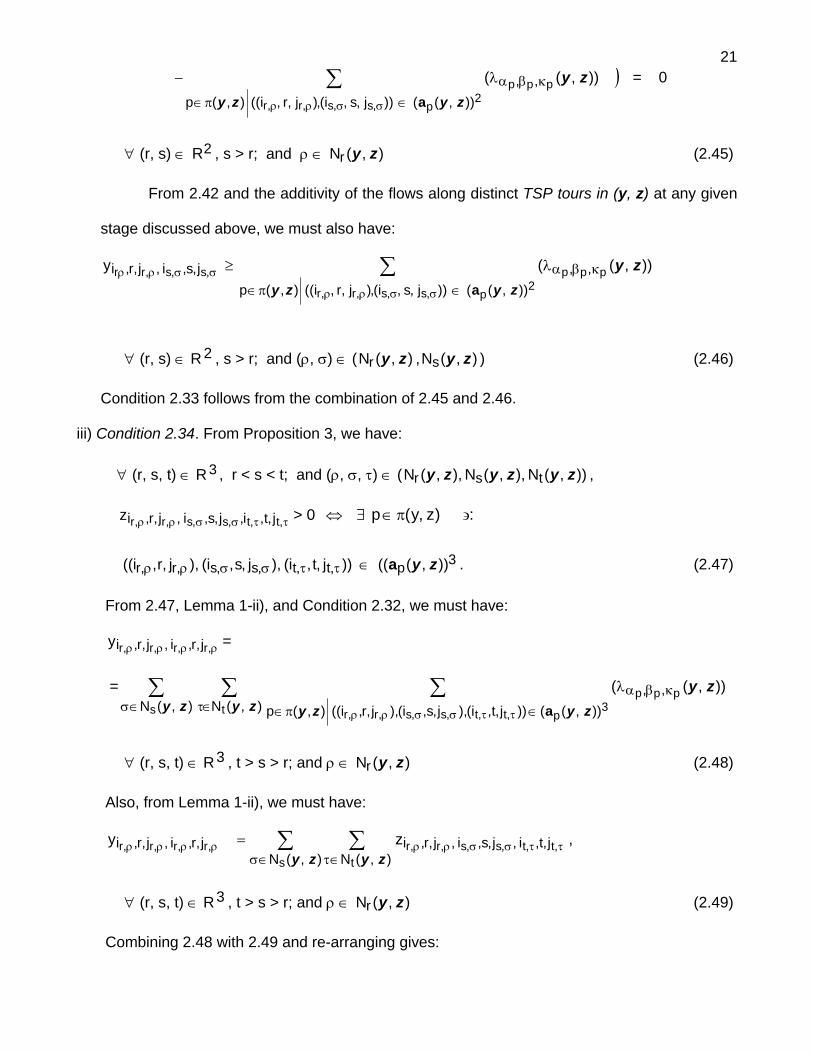
iii) Condition 2.34. From Proposition 3, we have:
∀ (r, s, t) ∈ R , r < s < t; and (ρ, σ, τ) ∈ ( ,
> 0
3 )),(N),,(N),,(N tsr zyzyzy
ττσσρρ ,t,t,s,s,r,r j,t,i,j,s,i,j,r,iz ⇔ )z,y(p π∈∃ :∋
. (2.47) 3p,t,t,s,s,r,r )),((())j,t,i(),j,s,i(),j,r,i(( zya∈ττσσρρ
From 2.47, Lemma 1-ii), and Condition 2.32, we must have:
ρρρρ ,r,r,r,r j,r,i,j,r,iy =
= ∑ ∑ ∑∈σ ∈τ ∈π∈
κβα
ττσσρρ
λ),(N ),(N )),(())j,t,i(),j,s,i(),j,r,i((),(p
,,s t 3
p,t,t,s,s,r,r
ppp )),((zy zy zyzy
zya
∀ (r, s, t) ∈ R3 , t > s > r; and ρ ∈ (2.48) ),(Nr zy
Also, from Lemma 1-ii), we must have:
∑ ∑∈σ ∈τ
ττσσρρρρρρ =),(N ),(N
j,t,i,j,s,i,j,r,ij,r,i,j,r,is t
,t,t,s,s,r,r,r,r,r,r zyzy zy
,
∀ (r, s, t) ∈ R3 , t > s > r; and ρ ∈ (2.49) ),(Nr zy
Combining 2.48 with 2.49 and re-arranging gives:

22( ττσσρρ∑ ∑
∈σ ∈τ,t,t,s,s,r,r
s tj,t,i,j,s,i,j,r,i
),(N ),(Nz
zy zy +
∑∈π∈
κβα
ττσσρρ
λ−3
p,t,t,s,s,r,r
ppp))(y,())j,t,i(),j,s,i(),j,r,i((),(p
,, ))((zzy
zy,a
) = 0
∀ (r, s, t) ∈ R3 , t > s > r; and ρ ∈ (2.50) ),(Nr zy
From 2.47 and the additivity of the flows along distinct TSP tours in (y, z) discussed
above, we must also have:
ττσσρρ ,t,t,s,s,r,r j,t,i,j,s,i,j,r,iz ≥
∑∈π∈
κβα
ττσσρρ
λ3
p,t,t,s,s,r,r
ppp))(())j,t,i(),j,s,i(),j,r,i((),(p
,, ))((zy,zy
zy,a
∀ (r, s, t) ∈ R3 , t > s > r; and (ρ, σ, τ) ∈ ( , , ) (2.51) ),(Nr zy ),(Ns zy ),(Nt zy
Condition 2.34 follows from the combination of 2.50 and 2.51.
Q.E.D.
Proposition 4 is illustrated in Figure 2.2, along with the notation discussed above.
----------------------------------------------- Figure 2.2 Here
------------------------------------------------
Proposition 5
The following statements are true of basic feasible solutions (BFS) of Problem BLP and TSP
tours:
1) Every BFS of Problem BLP corresponds to a TSP tour;
2) Every TSP tour corresponds to a BFS of Problem BLP;
3) The mapping of BFS’s of Problem BLP onto TSP tours is surjective.
Proof:
1) Correspondence of a BFS of Problem BLP to a TSP tour follows from the fact that every TSP
tour corresponds to a feasible solution to Problem BLP (Proposition 1), the fact that every
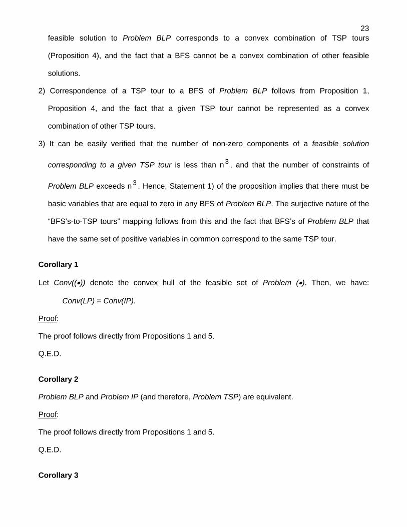
23feasible solution to Problem BLP corresponds to a convex combination of TSP tours
(Proposition 4), and the fact that a BFS cannot be a convex combination of other feasible
solutions.
2) Correspondence of a TSP tour to a BFS of Problem BLP follows from Proposition 1,
Proposition 4, and the fact that a given TSP tour cannot be represented as a convex
combination of other TSP tours.
3) It can be easily verified that the number of non-zero components of a feasible solution
corresponding to a given TSP tour is less than n3 , and that the number of constraints of
Problem BLP exceeds n . Hence, Statement 1) of the proposition implies that there must be
basic variables that are equal to zero in any BFS of Problem BLP. The surjective nature of the
“BFS’s-to-TSP tours” mapping follows from this and the fact that BFS’s of Problem BLP that
have the same set of positive variables in common correspond to the same TSP tour.
3
Corollary 1
Let Conv((•)) denote the convex hull of the feasible set of Problem (•). Then, we have:
Conv(LP) = Conv(IP).
Proof:
The proof follows directly from Propositions 1 and 5.
Q.E.D.
Corollary 2
Problem BLP and Problem IP (and therefore, Problem TSP) are equivalent.
Proof:
The proof follows directly from Propositions 1 and 5.
Q.E.D.
Corollary 3

24Computational complexity classes P and NP are equal.
Proof:
First, note that Problem BLP has O(n9) variables and O(n7) constraints. Hence, it can be explicitly
stated in polynomial time. The proposition follows from this, Corollary 2, the NP-Completeness of
the TSP decision problem (see Garey and Johnson [1979], or Nemhauser and Wolsey [1988],
among others), and the fact that an explicitly-stated instance of Problem BLP can be solved in
polynomial-time (see Katchiyan [1979], or Karmarkar [1984]).
Q.E.D.
3. Numerical Implementation
Note that because of Proposition 4, the upper bounds on the and variables in
constraints 2.18 are redundant in Problem BLP. Also, it is easy to observe that the visits
requirements constraints 2.12 – 2.13 are not used (and hence, are not needed) in any of the
proofs in section 2 of this paper. Hence, those constraints (i.e., constraints 2.12 - 2.13) are
redundant in Problem BLP (and therefore, in Problem IP). Hence, in implementing the model, we
discarded constraints 2.12 – 2.13 and replaced constraints 2.18 with simple non-negativity
constraints on the and variables. In addition, we did not explicitly consider
constraints 2.14 and the variables they restrict to zero. This required appropriately re-
writing/expanding the other constraints of the model. The resulting “streamlined” model that we
implemented is as follows:
irjksty irjupvkstz
irjksty irjupvkstz
Problem SLP:
Minimize
ZLP(y, z) = (3.1) ∑ ∑ ∑∈ ∈ ∈Rr Mi })i{\Mj
irjirjirjyc
Subject to:
• Flow Conservations (Corresponding to 2.6 and 2.7):

25
+−− − t,1p,vupvu,1p,iupvu,1p,i zy
∑ ∑∈ ∈Mi }i{\Mj
j,1,i,j,1,iy = 1 (3.2)
∑∈
−j}){i,\M(u
jii,2,u,1,j,2,ji,2,i yy = 0 i ∈ M; j ∈ M\{i} (3.3)
∑ ∑∈ ∈
−j}){i,\M(u u})j,{i,\M(v
virju,1,irjirj yy = 0 r ∈ R, r ≥ 3; i ∈ M; j ∈ M\{i} (3.4)
• Flow Connectivities (Corresponding to 2.8):
∑∈
+−j}){i,\M(t
t1,rirjj,irjirj yy = 0 r ∈ R, r ≤ n-3; i ∈ M; j ∈ M\{i} (3.5)
∑∈
++ −})t,j,i{\M(k
k,2r,irjtt,1r,irjj yy = 0 i ∈ M; j ∈ M\{i}; t ∈ M\{i,j};
r ∈ R, r ≤ n-4, (3.6)
∑∑∈
+∈
−Mk
k1,srjt,iMk
stkrji yy = 0 i, j, t ∈ M; s, r ∈ R,
r ≤ n-5, r+2 ≤ s ≤ n-3 (3.7)
• Flow Layering Consistencies A (Corresponding to 2.9):
∑∈ }v,u,i{\Mt
= 0 i ∈ M; u ∈ M\{i}; v ∈ M\{i,u};
p ∈ R, 2 ≤ p ≤ n-3 (3.8)
∑ ∑ −− −∈ ∈
kstupvu,1p,iupvu,1p,i zy
+− t,1p,vupvirjupvirj zy
}v,u,i{\Mk }k,v,u,i{\Mt= 0 i ∈ M; u ∈ M\{i}; v ∈ M\{i,u};
p, s ∈ R, 2 ≤ p ≤ n-4, s ≥ p+2 (3.9)
∑∈ }v,u,j,i{\Mt
= 0 i ∈ M; j ∈ M\{i}; u ∈ M\{i,j}; v ∈ M\{i,j,u};
p, r ∈ R, 3 ≤ p ≤ n-3, r ≤ p-2 (3.10)
∑ ∑−∈ ∈
kstupvirjupvirj zy
• Flow Layering Consistencies B (Corresponding to 2.11):
t,2r,kk,1r,jirjt,2r,kirj +++ = 0 i ∈ M; j ∈ M\{i}; k ∈ M\{i, j}; t ∈ M\{i,j,k};
}v,u,j,i{\Mk }k,v,u,j,i{\Mt= 0 i ∈ M; j ∈ M\{i}; u ∈ M\{i, j}; v ∈ M\{i,j, u};
p, r, s ∈ R, 3 ≤ p ≤ n-4, r ≤ p-2, s ≥ p+2 (3.11)
zy −

26 r ∈ R, r ≤ n-4 (3.12)
∑∈
+−}t,k,j,i{\Mv
kstv,1r,jirjkstirj zy = 0 i ∈ M; j ∈ M\{i}; k ∈ M\{i, j}; t ∈ M\{i,j, k};
r, s ∈ R, r ≤ n-5, s ≥ r+3 (3.13)
∑∈
−−}t,k,j,i{\Mu
kstk,1s,uirjkstirj zy = 0 i ∈ M; j ∈ M\{i}; k ∈ M\{i,j}; t ∈ M\{i,j,k}
r, s ∈ R, r ≤ n-5, s ≥ r+3 (3.14)
∑ ∑∈ ∈
−}t,k,j,i{\Mu }u,t,k,j,i{\Mv
kstupvirjkstirj zy = 0 i ∈ M; j ∈ M\{i}; k ∈ M\{i, j}; t ∈ M\{i,j, k}; p, r, s ∈ R,
r ≤ n-6, s ≥ r+4 r+2 ≤ p ≤ s -2 (3.15)
• Flow Layering Consistencies C (Corresponding to 2.11):
∑∈
+−+ −}t,v,u{\Mi
t,1p,vupvu,1p,it,1p,vupv zy = 0 u ∈ M; v ∈ M\{u}; t ∈ M\{u,v};
p ∈ R, 2 ≤ p ≤ n-3 (3.16)
∑ ∑∈ ∈
++ −}t,v,u{\Mi }i,t,v,u{\Mj
t,1p,vupvirjt,1p,vupv zy = 0 u ∈ M; v ∈ M\{u}; t ∈ M\{u,v};
p, r ∈ R, 3 ≤ p ≤ n-3, r ≤ p-2 (3.17)
∑∈
−−}t,k,v,u{\Mi
kstupvu,1p,iupvkst zy = 0 u ∈ M; v ∈ M\{u}; k ∈ M\{u, v}; t ∈ M\{u,v,k}
p, s ∈ R, 2 ≤ p ≤ n-4, s ≥ p+2 (3.18)
∑ ∑∈ ∈
−}t,k,v,u{\Mi }i,t,k,v,u{\Mj
kstupvirjupvkst zy = 0 u ∈ M; v ∈ M\{u}; k ∈ M\{u, v}; t ∈ M\{u,v,k};
p, r, s ∈ R, 3 ≤ p ≤ n-4; r ≤ p-2, s ≥ p+2 (3.19)
• Non-negativities (Corresponding to (2.18)):
irjksty , ≥ 0 ∀ i, r, j, u, p, v, k, s, t (3.20) irjupvkstz
We used the simplex method implementation of the OSL optimization package (IBM) to
solve a set of randomly-generated 7-city and 8-city problems. The travel costs in these randomly-
generated problems were taken as uniform integer numbers between 1 and 300. For each
problem size, 3 instances had symmetric costs, and 3 instances had asymmetric costs. We also

27solved an additional set of 7-city problems we refer to as “extreme-symmetry” problems. These
“extreme-symmetry” problems are labeled “xtsp71,” “xtsp72,” and “xtsp73,” respectively. In
Problem xtsp71, all travel costs, , are equal to (-1), except for tijt 12 and t21 which are equal to 1,
respectively. In Problem xtsp72, all travel costs, , are equal to 1, except for tijt 12 and t21 which are
equal to (-100), respectively. Finally, in Problem xtsp73, all travel costs, , are equal to 0, except
for t
ijt
12 and t21 which are equal to 1, respectively.
We solved each of the test problems described above using their dual forms, respectively.
We also solved the primal forms of the 7-city problems. The costs data and solutions obtained
using the dual forms (except for Problems xtsp71 and xtsp73) are shown in Appendix A of this
paper. Details of the solutions from the dual forms for Problems xtsp71 and xtsp73, respectively,
are given in Appendices B through E. The computational results are summarized in Tables 3.1
and 3.2, for the dual and primal forms, respectively.
Using the dual forms, the averages of the numbers of iterations for the 7-city problems
were 592.7, 1,825.7, and 8,433.3 for the asymmetric, symmetric, and “extreme-symmetry”
problems, respectively. The corresponding average computational times were 0.0993, 0.3230,
and 14.5523 CPU seconds of Sony VAIO VGN-FE 770G notebook computer (1.8 GHz Intel Core
2 Duo Processor) time, respectively. For the 8-city problems the averages of the numbers of
iterations were 19,622.3 and 42,082.7 for the asymmetric and symmetric problems, respectively.
The corresponding average computational times were 182.4433 and 700.9897 CPU seconds,
respectively.
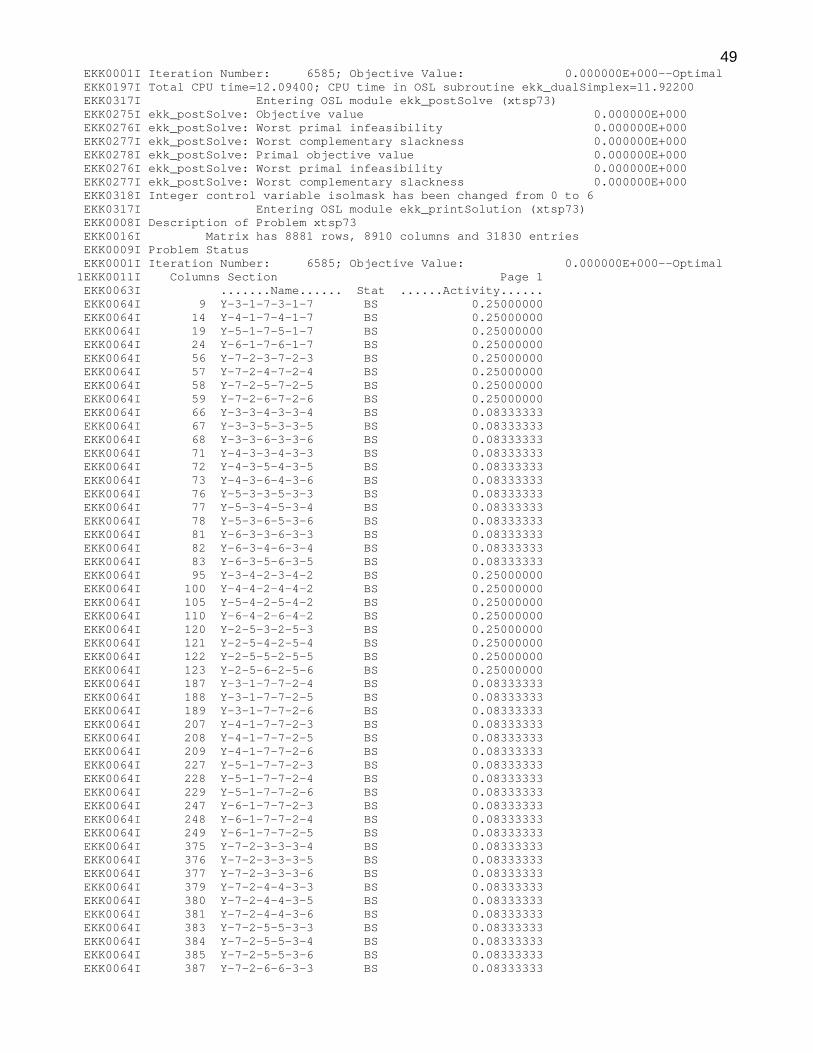
For the “extreme-symmetry” Problems xtsp71 and xtsp73, the simplex method using the
dual forms stopped with optimal, but non-extreme-point solutions, respectively. It appears from
the OSL outputs for these problems (shown in Appendices B and D, respectively) that this may
be due to numerical difficulties. Note also, that in both cases the solutions obtained (using the
dual form) are consistent with Proposition 4 of section 2 of this paper in that they respectively are

28indeed convex combinations of feasible solutions corresponding to TSP tours. The TSP tours that
comprise the solution obtained for Problem xtsp71 are: 1→3→6→2→4→7→5→1,
1→3→6→4→2→5→7→1, 1→6→3→2→4→5→7→1, and 1→6→3→4→2→7→5→1,
respectively, each with “weight” (or, flow value) λ = 0.25 (see Appendix C). Similarly, the solution
obtained using the dual form for Problem xtsp73 consists of the twelve (12) TSP tours shown in
Appendix E. Hence, we believe that these solutions further validate, somewhat, our Proposition 4
in particular. Finally, note that the TSP tours that comprise any given feasible solution to our LP
model, as stipulated by Proposition 4, can be systematically identified in a straightforward manner
using the “paths” defined/developed in section 2 of this paper. Hence, an optimal TSP tour can be
retrieved from any given (feasible) non-extreme-point optimum in a straightforward manner.
For the primal forms, the average number of iterations was 10,862.3, 13,996.7, and
19,858.3 for the asymmetric, symmetric, and “extreme-symmetry” problems, respectively. The
corresponding average computational times were 28.7080, 40.4533, and 62.2340 CPU seconds,
respectively. The average number of TSP tours examined in the simplex procedure was 2.3, 1.3,
and 1.0 for the asymmetric, symmetric, and “extreme-symmetry” problems, respectively.
Overall, we believe our computational experience provided the empirical validation of our
theoretical developments in section 2 of this paper that we expected. The dual forms consistently
outperformed the primal forms. However, the primal form appears to hold some promise with
respect to future developments aimed at solving large-sized problems because of the small
number of TSP tours that are examined when the primal form is used. We believe that greater
overall computational performance may be achieved using the primal form if the simplex pivoting
step can be customized judiciously-enough to take advantage of the special (TSP tour) nature of
the basic feasible solutions of our proposed linear programming model.
4. Conclusions
We have presented a first polynomial-sized linear programming formulation of the TSP. Our

29approach can be used to formulate general integer programming problems as linear programs,
since the general integer programming problem is polynomially transformable to a Hamiltonian
Path problem (see Johnson and Papadimitriou [1985, pp. 61-74]. Note however, that the
Hamiltonian Path problem resulting from the transformation involved is very-large-scale. Hence,
we believe a key issue at this point is the question of whether the suggested modeling approach
can be developed into a more general, unified framework that would extend in a more natural way
to other NP-Complete problems (see Garey and Johnson [1979], or Nemhauser and Wolsey
[1988], among others).

30
s=n-1s=1 s=2 s=n-2
i = 2
i = 3
i =n-1
i = n
j, s+1i, s xisj j, s+1i, s xisj
Figure 2.1: Illustration of the Network Sub-Structure of Problem TSP

31
• Graphical illustration of a feasible solution
• Graph theoretical notation G(y, z) = (V(y, z), A(y, z)); V(y, z) = {(4,1), (3,2), (5,3), (2,4), (6,4), (7,5), (2,6A(y, z) = {(4,1,3), (3,2,5), (5,3,2), (5,3,6), (2,4,7), (6,4,7), (7,5,2), (7,5,6)}.
), (6,6)},
1X (y, z) = { (4,1,3) }; y, z) = { (3,2,5) }; y, z) = { (5,3,1), (5,3,6 }; 2 3( , ) ( , ) = { (7,5,1), (7,5,6 }.
X ( X (
4X y z = { (1,4,7), (6,4,7 }; 5X y z
• on- onVector y (n zero comp ents) y = y = λ + λ = 1;413413 325325 1,1,1 1,2,1 y532532 = y247247 = y756756 = λ1,1,1;
y λ1,2,1; + = 1
y325647 = y325752 = y536647 = y536752 = y647752 = λ1,2,1.
•
y536536 = y647647 = 752752 = y413325 = λ1,1,1 λ1,2,1
y413532 = y413247 = y413756 = y325532 = y325247 = y325756 = y532247 = y532752 = y247756 = λ1,1,1; y413536 = y413647 = y413752 = y325536 =
Vector z (non-zero components) z413 325 532 = z413 325 247 = z413 325 756 = z413 532 247 = z413 532 752 = z413 247 756 = λ1,1,1;
3 647 752 = λ1,2,1;
52 = z325 647 752 = λ1,2,1; z536 647 752 = λ1,2,1.
•
z325 532 247 = z325 532 756 = z 325 247 756 = λ1,1,1; z532 247 756 = λ1,1,1; z413 325 536 = z413 325 647 = z413 325 752 = z413 536 647 = z413 536 752 = z41
z325 536 647 = z325 536 7
TSP Tours in (y, z) T1,1,1 = , 5, 2, 7, 6 ⟩, flow value = λ1,1,1; L1,2,1 = ⟨ 4, 3, 5, 6, 7, 2 ⟩, flow value = λ1,2,1.
Figure 2.2: Illustration of a Feasible Solution to Problem BLP
⟨ 4, 3
s=1 s=2 s=3 s=4 s=5 s=6
j = 2
j = 3
j = 4
j = 5
j = 6
j = 7

32
Computational Performance Problem
Size1Problem Name2
Number of Iterations
CPU Seconds3
Problem Value
atsp71 774 0.141 414
atsp72 605 0.094 468
atsp73 399 0.063 354
Average 592.7 0.0993 ---
stsp71 1,710 0.297 503
stsp72 2,091 0.375
1: (a): number of cities; (b): number of variables; (c): number of constraints
2: “atsp⋅⋅” ⇒ asymmetric costs; “stsp⋅⋅” ⇒ symmetric costs;
“xtsp⋅⋅” ⇒ “extreme symmetry” problem
3: Sony VAIO VGN-FE 770G notebook computer (1.8 GHz Intel Core 2 Duo Processor)
4: Non-extreme-point optimal solution
Table 3.1: Summary of the Computational Results for the Dual Forms
531
stsp73 1,676 0.297 637
Average 1,825.7 0.3230 ---
xtsp71 9,914 19.563 (-7) (4)
xtsp72 8,801 12.172 (-94)
xtsp73 6,585 11.922 0 (4)
7a
(8,910b; 8881c)
Average 8,433.3 14.5523 ---
atsp81 23,297 265.157 331
atsp82 20,967 212.157 371
atsp83 14,603 70.016 608
Average 19,622.3 182.4433 ---
stsp81 30,452 452.890 411
stsp82 65,507 1,299.454 799
stsp85 30,289 350.625 707
8
(63,462b; 40,321c)
Average 42,082.7 700.9897 ---

33
Computational Performance Problem
Size1Problem Name2
Number of Tours3
Number of Iterations
CPU Seconds4
Problem Value
atsp71 2 9,413 22.781 414
atsp72 2 4,327 4.109 468
atsp73 3 18,847 59.234 354
Average 2.3 10,862.3 28.7080 ---
stsp71 2 8,959 21.891 503
stsp72 1 10,542 26.859 531
stsp73 1 22,489 72.610 637
Average 1.3 13,996.7 40.4533 ---
xtsp71 1 8,264 17.984 (-7)
xtsp72 1 37,698 130.828 (-94)
xtsp73 1 13,613 37.890 0
7a
(8,910b; 8,881c)
Average 1.0 19,858.3 62.2340 ---
1: (a): number of cities; (b): number of variables; (c): number of constraints
2: “atsp⋅⋅” ⇒ asymmetric costs; “stsp⋅⋅” ⇒ symmetric costs;
“xtsp⋅⋅” ⇒ “extreme symmetry” problem
3: Total number of TSP tours (including the optimal tour) examined
4: Sony VAIO VGN-FE 770G notebook computer (1.8 GHz Intel Core 2 Duo Processor)
Table 3.2: Summary of the Computational Results for the Primal Forms
34References
Bazaraa, M.S., J.J. Jarvis, and H.D. Sherali, Linear Programming and Network Flows (Wiley, New York, 1990).
Dantzig, G.B., D.R. Fulkerson, and S.M. Johnson, “Solution of a large-scale traveling-salesman problem,” Operations Research 2 (1954) pp. 393-410.
Evans, J.R. and E. Minieka, Optimization Algorithms for Networks and Graphs (Marcel Dekker, New York, 1992).
Garey, M.R. and D.S. Johnson, Computers and Intractability: A Guide to the Theory of NP-Completeness (Freeman, San Francisco, 1979).
Grötschel, M. and M. W. Padberg, “Polyhedral Theory,” in: Lawler, E.L., J.K. Lenstra, A.H.G. Rinnooy Kan, and D.B. Shmoys, eds, The Traveling Salesman Problem: A Guided Tour of Combinatorial Optimization (Wiley, New York, 1985) pp. 251-305.
Johnson, D.S. and C.H. Papadimitriou, “Computational Complexity,” in: Lawler, E.L., J.K. Lenstra, A.H.G. Rinnooy Kan, and D.B. Shmoys, eds, The Traveling Salesman Problem: A Guided Tour of Combinatorial Optimization (Wiley, New York, 1985) pp. 37-85.
Karmarkar, N., “A new polynomial-time algorithm for linear programming,” Combinatorica 4 (1984) pp. 373-395.
Khachiyan, L.G., “A Polynomial algorithm in linear programming,” Soviet Mathematics Doklady 20 (1979) pp. 191-194.
Lawler, E.L., J.K. Lenstra, A.H.G. Rinnooy Kan, and D.B. Shmoys, eds, The Traveling Salesman Problem: A Guided Tour of Combinatorial Optimization (Wiley, New York, 1985).
Nemhauser, G.L. and L.A. Wolsey, Integer and Combinatorial Optimization, (Wiley, New York, 1988).
Padberg, M. W. and M. Grötschel, “Polyhedral Computations,” in: Lawler, E.L., J.K. Lenstra, A.H.G. Rinnooy Kan, and D.B. Shmoys, eds, The Traveling Salesman Problem: A Guided Tour of Combinatorial Optimization (Wiley, New York, 1985) pp. 307-360.
Padberg, M. and T.-Y. Sung, “An analytical comparison of diffferent formulations of the traveling salesman problem,” Mathematical Programming 52 (1991) pp. 315-357.
Yannakakis, M., “Expressing Combinatorial Optimization Problems by Linear Programs,” Journal of Computer and System Sciences 43 (1991) pp. 441-466.

35
Appendix A:
Cost and Solution* Data for the
Test Problems Solved
(*: All reported solutions are from the dual-form runs, unless indicated otherwise)

36
1 2 3 4 5 6 7 Cost 1 5000 181 157 91 209 153 100 100 2 180 5000 240 141 139 65 286 141 3 143 272 5000 45 127 20 121 20 4 40 63 212 5000 144 129 94 40 5 199 182 14 140 5000 281 16 14 6 293 61 79 164 287 5000 296 61 7 51 108 78 247 38 146 5000 38
Optimal Tour: 1 - 7 - 5 - 3 - 6 - 2 - 4 - 1 414
Table A.1: Cost Data and Solution Information for Problem atsp71
1 2 3 4 5 6 7 Cost 1 5000 267 79 46 284 167 219 46 2 222 5000 213 242 155 115 157 115 3 32 107 5000 102 195 216 232 32 4 184 29 116 5000 73 281 177 73 5 190 10 174 200 5000 280 40 10 6 161 238 165 86 243 5000 72 72 7 65 227 120 220 139 163 5000 120
Optimal Tour: 1 - 4 - 5 - 2 - 6 - 7 - 3 - 1 468
Table A.2: Cost Data and Solution Information for Problem atsp72
1 2 3 4 5 6 7 Cost 1 5000 40 15 248 68 12 258 68 2 39 5000 98 298 296 223 144 144 3 2 130 5000 202 285 178 278 2 4 197 221 71 5000 2 287 252 71 5 58 41 172 297 5000 140 174 41 6 151 218 237 23 146 5000 155 23 7 209 266 236 106 196 5 5000 5
Optimal Tour: 1 - 5 - 2 - 7 - 6 - 4 - 3 - 1 354
Table A.3: Cost Data and Solution Information for Problem atsp73

37
1 2 3 4 5 6 7 Cost 1 5000 173 149 83 201 145 92 149 2 173 5000 172 232 133 131 57 133 3 149 172 5000 277 135 263 37 37 4 83 232 277 5000 119 12 113 83 5 201 133 135 119 5000 32 55 32 6 145 131 263 12 32 5000 204 12 7 92 57 37 113 55 204 5000 57
Optimal Tour: 1 - 3 - 7 - 2 - 5 - 6 - 4 - 1 503
Table A.4: Cost Data and Solution Information for Problem stsp71
1 2 3 4 5 6 7 Cost 1 5000 48 23 257 76 20 266 20 2 48 5000 47 106 7 5 231 7 3 23 47 5000 152 10 138 211 23 4 257 106 152 5000 293 186 286 106 5 76 7 10 293 5000 205 229 10 6 20 5 138 186 205 5000 79 79 7 266 231 211 286 229 79 5000 286
Optimal Tour: 1 - 6 - 7- 4 - 2 - 5 - 3 - 1 531
Table A.5: Cost Data and Solution Information for Problem stsp72
1 2 3 4 5 6 7 Cost 1 5000 33 8 241 60 5 251 8 2 33 5000 31 91 291 289 215 91 3 8 31 5000 137 293 123 195 31 4 241 91 137 5000 277 171 271 171 5 60 291 293 277 5000 190 213 60 6 5 289 123 171 190 5000 63 63 7 251 215 195 271 213 63 5000 213
Optimal Tour: 1 - 3 - 2 - 4 - 6 - 7 - 5 - 1 637
Table A.6: Cost Data and Solution Information for Problem stsp73

38
1 2 3 4 5 6 7 Cost 1 5000 1 0 0 0 0 0 0 2 1 5000 0 0 0 0 0 0 3 0 0 5000 0 0 0 0 0 4 0 0 0 5000 0 0 0 0 5 0 0 0 0 5000 0 0 0 6 0 0 0 0 0 5000 0 0 7 0 0 0 0 0 0 5000 0
Optimal Tour: 1 - 6 - 4 – 2 - 5 - 3 - 7 - 1 0
Table A.7: Cost Data and Solution Information for Problem xtsp71 (Solution from Primal Form)
1 2 3 4 5 6 7 Cost 1 5000 -100 1 1 1 1 1 -100 2 -100 5100 1 1 1 1 1 1 3 1 1 5000 1 1 1 1 1 4 1 1 1 5000 1 1 1 1 5 1 1 1 1 5000 1 1 1 6 1 1 1 1 1 5000 1 1 7 1 1 1 1 1 1 5000 1
Optimal Tour: 1 - 2 - 6 - 7- 5 - 3 - 4 - 1 -94
Table A.8: Cost Data and Solution Information for Problem xtsp72
1 2 3 4 5 6 7 Cost 1 5000 1 -1 -1 -1 -1 -1 -1 2 1 5000 -1 -1 -1 -1 -1 -1 3 -1 -1 5000 -1 -1 -1 -1 -1 4 -1 -1 -1 5000 -1 -1 -1 -1 5 -1 -1 -1 -1 5000 -1 -1 -1 6 -1 -1 -1 -1 -1 5000 -1 -1 7 -1 -1 -1 -1 -1 -1 5000 -1
Optimal Tour: 1 - 3 - 2 - 5 - 6 – 4 - 7 - 1 -7
Table A.9: Cost Data and Solution Information for Problem xtsp73 (Solution from Primal Form)

39
1 2 3 4 5 6 7 8 Cost 1 5000 108 84 18 136 80 27 107 27 2 167 5000 68 66 291 213 70 199 68 3 271 54 5000 247 48 266 289 139 48 4 71 56 21 5000 126 109 240 67 71 5 208 242 220 287 5000 6 91 215 6 6 223 277 35 5 174 5000 264 73 73 7 189 1 267 206 89 141 5000 144 1 8 135 163 77 37 78 253 29 5000 37
Optimal Tour: 1 - 7 - 2 - 3 - 5 - 6 - 8 - 4 - 1 331
Table A.10: Cost Data and Solution Information for Problem atsp81
1 2 3 4 5 6 7 8 Cost 1 5000 125 101 35 153 97 44 124 35 2 184 5000 85 83 9 229 87 215 9 3 288 71 5000 263 65 283 7 156 7 4 88 73 38 5000 143 126 257 84 38 5 225 259 237 5 5000 23 108 231 23 6 240 294 52 22 191 5000 281 90 90 7 206 17 284 223 106 158 5000 161 17 8 152 180 94 54 95 270 45 5000 152
Optimal Tour: 1 - 4 - 3 - 7 - 2 - 5 - 6 - 8 - 1 371
Table A.11: Cost Data and Solution Information for Problem atsp82
1 2 3 4 5 6 7 8 Cost 1 5000 223 198 132 250 195 142 221 132 2 281 5000 182 180 106 28 184 14 14 3 86 168 5000 62 162 81 105 253 162 4 185 170 135 5000 241 223 55 181 55 5 23 57 35 102 5000 120 206 30 57 6 38 93 149 119 289 5000 80 188 38 7 4 115 82 21 204 255 5000 259 82 8 249 278 192 151 193 68 143 5000 68
Optimal Tour: 1 - 4 - 7 - 3 - 5 - 2 - 8 - 6 - 1 608
Table A.12: Cost Data and Solution Information for Problem atsp83

40
1 2 3 4 5 6 7 8 Cost 1 5000 143 118 52 170 115 62 141 62 2 143 5000 201 102 100 26 247 104 26 3 118 201 5000 233 6 88 281 82 82 4 52 102 233 5000 1 24 173 105 52 5 170 100 6 1 5000 90 55 161 6 6 115 26 88 24 90 5000 143 274 24 7 62 247 281 173 55 143 5000 101 55 8 141 104 82 105 161 274 101 5000 104
Optimal Tour: 1 - 7 - 5 - 3 - 8 - 2 - 6 - 4 - 1 411
Table A.13: Cost Data and Solution Information for Problem stsp81
1 2 3 4 5 6 7 8 Cost 1 5000 226 201 135 254 198 145 225 225 2 226 5000 284 185 183 110 31 188 31 3 201 284 5000 17 90 172 65 165 90 4 135 185 17 5000 84 108 257 189 135 5 254 183 90 84 5000 174 139 244 84 6 198 110 172 108 174 5000 227 59 110 7 145 31 65 257 139 227 5000 185 65 8 225 188 165 189 244 59 185 5000 59
Optimal Tour: 1 - 8 - 6 - 2 - 7 - 3 - 5 - 4 - 1 799
Table A.14: Cost Data and Solution Information for Problem stsp82
1 2 3 4 5 6 7 8 Cost 1 5000 214 190 124 242 186 133 213 213 2 214 5000 273 174 172 98 20 176 20 3 190 273 5000 6 78 160 54 154 78 4 124 174 6 5000 73 96 245 177 124 5 242 172 78 73 5000 162 127 232 73 6 186 98 160 96 162 5000 215 47 98 7 133 20 54 245 127 215 5000 173 54 8 213 176 154 177 232 47 173 5000 47
Optimal Tour: 1 - 8 - 6 - 2 - 7 - 3 - 5 - 4 - 1 707
Table A.15: Cost Data and Solution Information for Problem stsp83

41
Appendix B:
OSL Outputs for the Dual Form of Problem xtsp71

42EKK0330I New logfile is .\TSPLP\Outputs\xtsp71D.txt EKK0317I Entering OSL module ekk_importModelFree () EKK0078I 1 NAME xtsp71 FREE EKK0185I ekk_importModelFree will read this file in free format EKK0078I 2 ROWS EKK0078I 8885 COLUMNS EKK0078I 40856 RHS EKK0078I 40858 ENDATA EKK0014I Using Matrix xtsp71 EKK0014I Using Objective LP_Obj EKK0014I Using RHS rhs(1) EKK0016I Matrix has 8881 rows, 8910 columns and 31830 entries EKK0019I There are 140 objective row entries EKK0197I Total CPU time=0.1410000; CPU time in OSL subroutine ekk_importModelFree=0.1410000 EKK0317I Entering OSL module ekk_scale (xtsp71) EKK0021I The initial range of the matrix coefficients is 1.000000 - 1.000000 EKK0023I OSL subroutine ekk_scale is creating a new copy of the matrix or is modifying an old copy EKK0317I Entering OSL module ekk_preSolve (xtsp71) EKK0026I After presolving the matrix, there are 7685 active columns, 7656 active rows, and 29105 active elements EKK0023I OSL subroutine ekk_preSolve is creating a new copy of the matrix or is modifying an old copy EKK0317I Entering OSL module ekk_dualSimplex (xtsp71) EKK0038I Iterations/Objective Primal/Dual Infeasibilities EKK0057I 0 0.000000E+000 1.0000000( 1) 1640.000( 1140) EKK0057I 188 -3.000000 109.8000( 196) 839.9999( 540) EKK0057I 376 -4.000000 141.2000( 301) 812.7499( 545) EKK0057I 564 -4.000000 145.1667( 420) 812.7499( 545) EKK0057I 752 -4.155280 307.6242( 835) 783.4906( 731) EKK0057I 940 -4.298487 330.8847( 870) 764.5193( 688) EKK0057I 1128 -4.430100 712.7988( 1185) 748.9151( 664) EKK0057I 1316 -5.438122 2572.205( 1240) 682.1998( 634) EKK0057I 1504 -5.972183 1837.227( 1361) 654.9869( 640) EKK0057I 1692 -6.546775 1531.542( 1608) 577.7235( 581) EKK0057I 1880 -6.900262 1352.695( 1698) 553.4781( 561) EKK0057I 2068 -7.299845 1147.476( 1828) 486.9874( 542) EKK0057I 2256 -7.507376 940.7844( 2016) 444.7846( 480) EKK0057I 2444 -7.667893 2959.317( 2218) 414.3482( 438) EKK0057I 2632 -7.779031 1457.246( 2250) 384.6767( 435) EKK0057I 2820 -7.849022 1100.049( 2328) 362.1770( 432) EKK0057I 3008 -7.902891 1540.380( 2333) 352.4042( 422) EKK0057I 3196 -8.071280 2207.014( 2611) 333.2466( 439) EKK0057I 3384 -8.226040 1300.982( 2729) 314.5320( 407) EKK0057I 3572 -8.360975 826.9534( 2851) 296.3863( 393) EKK0038I Iterations/Objective Primal/Dual Infeasibilities EKK0057I 3760 -8.496420 6137.426( 2932) 260.7155( 395) EKK0057I 3948 -8.810094 1212.428( 3028) 237.1471( 348) EKK0057I 4136 -9.329431 3440.589( 3320) 206.1470( 296) EKK0057I 4324 -9.606298 1793.925( 3283) 183.2834( 272) EKK0057I 4512 -9.730574 1246.524( 3305) 162.1169( 261) EKK0057I 4700 -9.848850 1569.965( 3402) 139.5732( 248) EKK0057I 4888 -9.938386 1112.217( 3392) 115.0372( 230) EKK0057I 5076 -9.972635 3254.101( 3485) 84.54723( 192) EKK0057I 5264 -9.978044 1830.853( 3476) 59.18764( 157) EKK0057I 5452 -9.913020 1098.767( 3474) 45.78632( 138) EKK0057I 5640 -9.934679 3209.067( 3533) 34.31379( 94) EKK0057I 5828 -10.11241 6244.435( 3555) 21.53697( 83) EKK0057I 6016 -10.37490 4169.223( 3655) 11.39882( 44) EKK0057I 6204 -10.55943 1694.127( 3663) 5.927413( 31) EKK0057I 6392 -10.55018 1402.171( 3646) 1.514788( 9) EKK0057I 6580 -10.02637 18287.54( 3692) 0.000000E+000( 0)

43 EKK0057I 6768 -9.524849 4415.787( 3605) 0.000000E+000( 0) EKK0057I 6949 -9.105607 1363.484( 3680) 0.000000E+000( 0) EKK0057I 7120 -8.864572 5886.949( 3710) 0.000000E+000( 0) EKK0057I 7295 -8.636312 12902.63( 3733) 0.000000E+000( 0) EKK0038I Iterations/Objective Primal/Dual Infeasibilities EKK0057I 7457 -8.375790 8882.901( 3729) 0.000000E+000( 0) EKK0057I 7634 -8.077060 5406.381( 3677) 0.000000E+000( 0) EKK0057I 7809 -7.000000 1226.547( 3695) 0.000000E+000( 0) EKK0057I 7963 -7.000000 397.1772( 3725) 0.000000E+000( 0) EKK0057I 8122 -7.000000 236.0282( 3709) 0.000000E+000( 0) EKK0057I 8297 -7.000000 107.7196( 3693) 0.000000E+000( 0) EKK0057I 8471 -7.000000 134.6710( 3649) 0.000000E+000( 0) EKK0057I 8640 -7.000000 78.53908( 3563) 0.000000E+000( 0) EKK0057I 8828 -7.000000 110.0945( 3622) 0.000000E+000( 0) EKK0057I 9016 -7.000000 127.0596( 3687) 0.000000E+000( 0) EKK0057I 9204 -7.000000 58.69941( 3416) 0.000000E+000( 0) EKK0057I 9392 -7.000000 84.00530( 3507) 1.392577E-012( 1) EKK0057I 9580 -7.000000 80.00985( 3367) 0.000000E+000( 0) EKK0033I The problem has been perturbed EKK0057I 9768 -7.000000 80.19672( 3482) 0.000000E+000( 0) EKK0001I Iteration Number: 9914; Objective Value: -7.000000--Optimal EKK0197I Total CPU time=19.73500; CPU time in OSL subroutine ekk_dualSimplex=19.56300 EKK0317I Entering OSL module ekk_postSolve (xtsp71) EKK0275I ekk_postSolve: Objective value -7.000000 EKK0276I ekk_postSolve: Worst primal infeasibility 0.000000E+000 EKK0277I ekk_postSolve: Worst complementary slackness 0.000000E+000 EKK0278I ekk_postSolve: Primal objective value -7.000000 EKK0276I ekk_postSolve: Worst primal infeasibility 0.000000E+000 EKK0277I ekk_postSolve: Worst complementary slackness 0.000000E+000 EKK0318I Integer control variable isolmask has been changed from 0 to 6 EKK0317I Entering OSL module ekk_printSolution (xtsp71) EKK0008I Description of Problem xtsp71 EKK0016I Matrix has 8881 rows, 8910 columns and 31830 entries EKK0009I Problem Status EKK0001I Iteration Number: 9914; Objective Value: -7.000000--Optimal 1EKK0011I Columns Section Page 1 EKK0063I .......Name...... Stat ......Activity...... EKK0064I 8 Y-3-1-6-3-1-6 BS 0.50000000 EKK0064I 21 Y-6-1-3-6-1-3 BS 0.50000000 EKK0064I 35 Y-3-2-2-3-2-2 BS 0.25000000 EKK0064I 36 Y-3-2-4-3-2-4 BS 0.25000000 EKK0064I 50 Y-6-2-2-6-2-2 BS 0.25000000 EKK0064I 52 Y-6-2-4-6-2-4 BS 0.25000000 EKK0064I 61 Y-2-3-4-2-3-4 BS 0.50000000 EKK0064I 70 Y-4-3-2-4-3-2 BS 0.50000000 EKK0064I 92 Y-2-4-5-2-4-5 BS 0.25000000 EKK0064I 94 Y-2-4-7-2-4-7 BS 0.25000000 EKK0064I 102 Y-4-4-5-4-4-5 BS 0.25000000 EKK0064I 104 Y-4-4-7-4-4-7 BS 0.25000000 EKK0064I 139 Y-5-5-7-5-5-7 BS 0.50000000 EKK0064I 148 Y-7-5-5-7-5-5 BS 0.50000000 EKK0064I 182 Y-3-1-6-6-2-2 BS 0.25000000 EKK0064I 183 Y-3-1-6-6-2-4 BS 0.25000000 EKK0064I 234 Y-6-1-3-3-2-2 BS 0.25000000 EKK0064I 235 Y-6-1-3-3-2-4 BS 0.25000000 EKK0064I 290 Y-3-2-2-2-3-4 BS 0.25000000 EKK0064I 294 Y-3-2-4-4-3-2 BS 0.25000000 EKK0064I 351 Y-6-2-2-2-3-4 BS 0.25000000 EKK0064I 358 Y-6-2-4-4-3-2 BS 0.25000000 EKK0064I 395 Y-2-3-4-4-4-5 BS 0.25000000 EKK0064I 397 Y-2-3-4-4-4-7 BS 0.25000000 EKK0064I 431 Y-4-3-2-2-4-5 BS 0.25000000 EKK0064I 433 Y-4-3-2-2-4-7 BS 0.25000000 EKK0064I 521 Y-2-4-5-5-5-7 BS 0.25000000 EKK0064I 528 Y-2-4-7-7-5-5 BS 0.25000000 EKK0064I 561 Y-4-4-5-5-5-7 BS 0.25000000 EKK0064I 568 Y-4-4-7-7-5-5 BS 0.25000000

44 EKK0064I 918 Y-3-1-6-2-3-4 BS 0.25000000 EKK0064I 921 Y-3-1-6-4-3-2 BS 0.25000000 EKK0064I 931 Y-3-1-6-2-4-5 BS 0.25000000 EKK0064I 935 Y-3-1-6-4-4-7 BS 0.25000000 EKK0064I 950 Y-3-1-6-5-5-7 BS 0.25000000 EKK0064I 953 Y-3-1-6-7-5-5 BS 0.25000000 EKK0064I 1386 Y-6-1-3-2-3-4 BS 0.25000000 EKK0064I 1389 Y-6-1-3-4-3-2 BS 0.25000000 EKK0064I 1400 Y-6-1-3-2-4-7 BS 0.25000000 EKK0064I 1402 Y-6-1-3-4-4-5 BS 0.25000000 EKK0064I 1418 Y-6-1-3-5-5-7 BS 0.25000000 EKK0064I 1421 Y-6-1-3-7-5-5 BS 0.25000000 EKK0064I 1830 Y-3-2-2-4-4-5 BS 0.25000000 EKK0064I 1847 Y-3-2-2-5-5-7 BS 0.25000000 EKK0064I 1856 Y-3-2-4-2-4-7 BS 0.25000000 EKK0064I 1876 Y-3-2-4-7-5-5 BS 0.25000000 EKK0064I 2195 Y-6-2-2-4-4-7 BS 0.25000000 EKK0064I 2213 Y-6-2-2-7-5-5 BS 0.25000000 EKK0064I 2239 Y-6-2-4-2-4-5 BS 0.25000000 EKK0064I 2258 Y-6-2-4-5-5-7 BS 0.25000000 EKK0064I 2447 Y-2-3-4-5-5-7 BS 0.25000000 EKK0064I 2452 Y-2-3-4-7-5-5 BS 0.25000000 EKK0064I 2555 Y-4-3-2-5-5-7 BS 0.25000000 1EKK0011I Columns Section Page 2 EKK0063I .......Name...... Stat ......Activity...... EKK0064I 2560 Y-4-3-2-7-5-5 BS 0.25000000 EKK0064I 3120 Z(613322234) BS 0.25000000 EKK0064I 3123 Z(613322445) BS 0.25000000 EKK0064I 3132 Z(613322557) BS 0.25000000 EKK0064I 3180 Z(613324432) BS 0.25000000 EKK0064I 3184 Z(613324247) BS 0.25000000 EKK0064I 3194 Z(613324755) BS 0.25000000 EKK0064I 3990 Z(316622234) BS 0.25000000 EKK0064I 3994 Z(316622447) BS 0.25000000 EKK0064I 4004 Z(316622755) BS 0.25000000 EKK0064I 4125 Z(316624432) BS 0.25000000 EKK0064I 4128 Z(316624245) BS 0.25000000 EKK0064I 4137 Z(316624557) BS 0.25000000 EKK0064I 4674 Z(322234445) BS 0.25000000 EKK0064I 4678 Z(322234557) BS 0.25000000 EKK0064I 4694 Z(622234447) BS 0.25000000 EKK0064I 4700 Z(622234755) BS 0.25000000 EKK0064I 4715 Z(316234447) BS 0.25000000 EKK0064I 4716 Z(316234557) BS 0.25000000 EKK0064I 4734 Z(613234445) BS 0.25000000 EKK0064I 4737 Z(613234755) BS 0.25000000 EKK0064I 5432 Z(324432247) BS 0.25000000 EKK0064I 5437 Z(324432755) BS 0.25000000 EKK0064I 5449 Z(624432245) BS 0.25000000 EKK0064I 5454 Z(624432557) BS 0.25000000 EKK0064I 5470 Z(316432245) BS 0.25000000 EKK0064I 5473 Z(316432755) BS 0.25000000 EKK0064I 5491 Z(613432247) BS 0.25000000 EKK0064I 5492 Z(613432557) BS 0.25000000 EKK0064I 7235 Z(432245557) BS 0.25000000 EKK0064I 7245 Z(316245557) BS 0.25000000 EKK0064I 7281 Z(624245557) BS 0.25000000 EKK0064I 7354 Z(432247755) BS 0.25000000 EKK0064I 7381 Z(613247755) BS 0.25000000 EKK0064I 7386 Z(324247755) BS 0.25000000 EKK0064I 7832 Z(234445557) BS 0.25000000 EKK0064I 7857 Z(613445557) BS 0.25000000 EKK0064I 7873 Z(322445557) BS 0.25000000 EKK0064I 7951 Z(234447755) BS 0.25000000 EKK0064I 7973 Z(316447755) BS 0.25000000 EKK0064I 8005 Z(622447755) BS 0.25000000 EKK0317I Entering OSL module ekk_deleteModel (xtsp71)

45
Appendix C:
Summary of the TSP Tours Comprising the
Solution from the Dual Form of Problem xtsp71

46
TSP Tours Arcs of Graph G in the LP Solution
ID # Sequence Weight (3,1,6) (6,1,3) (3,2,2) (3,2,4) (6,2,2) (6,2,4) (2,3,4) (4,3,2)
1 1-3-6-2-4-7-5-1 0.25 1 1 1 2 1-3-6-4-2-5-7-1 0.25 1 1 1 3 1-6-3-2-4-5-7-1 0.25 1 1 1 4 1-6-3-4-2-7-5-1 0.25 1 1 1
Total Flow on Arc 0.50 0.50 0.25 0.25 0.25 0.25 .50 .50
Table C.1: Details of the TSP Tours in the Solution for the
Dual Form of Problem xtsp71- Part I
TSP Tours Arcs of Graph G in the LP Solution
ID # Sequence Weight (2,4,5) (2,4,7) (4,4,5) (4,4,7) (5,5,7) (7,5,5)
1 1-3-6-2-4-7-5-1 0.25 1 1 2 1-3-6-4-2-5-7-1 0.25 1 1 3 1-6-3-2-4-5-7-1 0.25 1 1 4 1-6-3-4-2-7-5-1 0.25 1 1
Total Flow on Arc 0.25 0.25 0.25 0.25 0.50 0.50
Table C.2: Details of the TSP Tours in the Solution for the
Dual Form of Problem xtsp71 - Part II

47
Appendix D:
OSL Outputs for the Dual Form of Problem xtsp73

48 EKK0330I New logfile is .\TSPLP\Outputs\xtsp73D.txt EKK0317I Entering OSL module ekk_importModelFree () EKK0078I 1 NAME xtsp73 FREE EKK0185I ekk_importModelFree will read this file in free format EKK0078I 2 ROWS EKK0078I 8885 COLUMNS EKK0078I 40726 RHS EKK0078I 40728 ENDATA EKK0014I Using Matrix xtsp73 EKK0014I Using Objective LP_Obj EKK0014I Using RHS rhs(1) EKK0016I Matrix has 8881 rows, 8910 columns and 31830 entries EKK0019I There are 10 objective row entries EKK0197I Total CPU time=0.1410000; CPU time in OSL subroutine ekk_importModelFree=0.1410000 EKK0317I Entering OSL module ekk_scale (xtsp73) EKK0021I The initial range of the matrix coefficients is 1.000000 - 1.000000 EKK0023I OSL subroutine ekk_scale is creating a new copy of the matrix or is modifying an old copy EKK0317I Entering OSL module ekk_preSolve (xtsp73) EKK0026I After presolving the matrix, there are 7705 active columns, 7676 active rows, and 29365 active elements EKK0023I OSL subroutine ekk_preSolve is creating a new copy of the matrix or is modifying an old copy EKK0317I Entering OSL module ekk_dualSimplex (xtsp73) EKK0038I Iterations/Objective Primal/Dual Infeasibilities EKK0057I 0 0.000000E+000 1.0000000( 1) 0.000000E+000( 0) EKK0057I 188 0.000000E+000 18.00000( 18) 0.000000E+000( 0) EKK0057I 376 0.000000E+000 35.00000( 163) 0.000000E+000( 0) EKK0057I 564 0.000000E+000 24.64865( 231) 0.000000E+000( 0) EKK0057I 752 0.000000E+000 23.44660( 454) 0.000000E+000( 0) EKK0057I 940 0.000000E+000 56.53779( 833) 0.000000E+000( 0) EKK0057I 1128 0.000000E+000 52.37572( 1011) 0.000000E+000( 0) EKK0057I 1316 0.000000E+000 55.31298( 1177) 0.000000E+000( 0) EKK0057I 1504 0.000000E+000 32.39207( 1338) 0.000000E+000( 0) EKK0057I 1692 0.000000E+000 51.67132( 1680) 0.000000E+000( 0) EKK0057I 1880 0.000000E+000 68.58153( 1793) 0.000000E+000( 0) EKK0057I 2068 0.000000E+000 61.22473( 1971) 0.000000E+000( 0) EKK0057I 2256 0.000000E+000 69.37150( 2049) 0.000000E+000( 0) EKK0057I 2444 0.000000E+000 86.25787( 2301) 0.000000E+000( 0) EKK0057I 2632 0.000000E+000 58.83881( 2317) 0.000000E+000( 0) EKK0057I 2820 0.000000E+000 120.1363( 2541) 0.000000E+000( 0) EKK0057I 3008 0.000000E+000 92.90198( 2685) 0.000000E+000( 0) EKK0057I 3196 0.000000E+000 92.50184( 2774) 0.000000E+000( 0) EKK0057I 3384 0.000000E+000 76.06881( 2937) 0.000000E+000( 0) EKK0057I 3572 0.000000E+000 59.77006( 2944) 0.000000E+000( 0) EKK0038I Iterations/Objective Primal/Dual Infeasibilities EKK0057I 3760 0.000000E+000 72.17296( 3001) 0.000000E+000( 0) EKK0057I 3948 0.000000E+000 72.28140( 3190) 0.000000E+000( 0) EKK0057I 4136 0.000000E+000 70.64216( 3213) 0.000000E+000( 0) EKK0057I 4324 0.000000E+000 57.71482( 3258) 0.000000E+000( 0) EKK0057I 4512 0.000000E+000 117.7179( 3386) 0.000000E+000( 0) EKK0057I 4700 0.000000E+000 102.5654( 3457) 0.000000E+000( 0) EKK0057I 4888 0.000000E+000 85.19144( 3430) 0.000000E+000( 0) EKK0057I 5076 0.000000E+000 53.51423( 3543) 0.000000E+000( 0) EKK0057I 5264 0.000000E+000 85.42116( 3600) 0.000000E+000( 0) EKK0057I 5452 0.000000E+000 64.88131( 3597) 0.000000E+000( 0) EKK0057I 5640 0.000000E+000 55.33657( 3615) 0.000000E+000( 0) EKK0057I 5828 0.000000E+000 96.87463( 3708) 0.000000E+000( 0) EKK0057I 6016 0.000000E+000 132.2508( 3836) 0.000000E+000( 0) EKK0057I 6204 0.000000E+000 30.17316( 3550) 0.000000E+000( 0) EKK0057I 6390 0.000000E+000 63.49333( 3790) 0.000000E+000( 0) EKK0057I 6578 0.000000E+000 77.24236( 3692) 0.000000E+000( 0)
49 EKK0001I Iteration Number: 6585; Objective Value: 0.000000E+000--Optimal EKK0197I Total CPU time=12.09400; CPU time in OSL subroutine ekk_dualSimplex=11.92200 EKK0317I Entering OSL module ekk_postSolve (xtsp73) EKK0275I ekk_postSolve: Objective value 0.000000E+000 EKK0276I ekk_postSolve: Worst primal infeasibility 0.000000E+000 EKK0277I ekk_postSolve: Worst complementary slackness 0.000000E+000 EKK0278I ekk_postSolve: Primal objective value 0.000000E+000 EKK0276I ekk_postSolve: Worst primal infeasibility 0.000000E+000 EKK0277I ekk_postSolve: Worst complementary slackness 0.000000E+000 EKK0318I Integer control variable isolmask has been changed from 0 to 6 EKK0317I Entering OSL module ekk_printSolution (xtsp73) EKK0008I Description of Problem xtsp73 EKK0016I Matrix has 8881 rows, 8910 columns and 31830 entries EKK0009I Problem Status EKK0001I Iteration Number: 6585; Objective Value: 0.000000E+000--Optimal 1EKK0011I Columns Section Page 1 EKK0063I .......Name...... Stat ......Activity...... EKK0064I 9 Y-3-1-7-3-1-7 BS 0.25000000 EKK0064I 14 Y-4-1-7-4-1-7 BS 0.25000000 EKK0064I 19 Y-5-1-7-5-1-7 BS 0.25000000 EKK0064I 24 Y-6-1-7-6-1-7 BS 0.25000000 EKK0064I 56 Y-7-2-3-7-2-3 BS 0.25000000 EKK0064I 57 Y-7-2-4-7-2-4 BS 0.25000000 EKK0064I 58 Y-7-2-5-7-2-5 BS 0.25000000 EKK0064I 59 Y-7-2-6-7-2-6 BS 0.25000000 EKK0064I 66 Y-3-3-4-3-3-4 BS 0.08333333 EKK0064I 67 Y-3-3-5-3-3-5 BS 0.08333333 EKK0064I 68 Y-3-3-6-3-3-6 BS 0.08333333 EKK0064I 71 Y-4-3-3-4-3-3 BS 0.08333333 EKK0064I 72 Y-4-3-5-4-3-5 BS 0.08333333 EKK0064I 73 Y-4-3-6-4-3-6 BS 0.08333333 EKK0064I 76 Y-5-3-3-5-3-3 BS 0.08333333 EKK0064I 77 Y-5-3-4-5-3-4 BS 0.08333333 EKK0064I 78 Y-5-3-6-5-3-6 BS 0.08333333 EKK0064I 81 Y-6-3-3-6-3-3 BS 0.08333333 EKK0064I 82 Y-6-3-4-6-3-4 BS 0.08333333 EKK0064I 83 Y-6-3-5-6-3-5 BS 0.08333333 EKK0064I 95 Y-3-4-2-3-4-2 BS 0.25000000 EKK0064I 100 Y-4-4-2-4-4-2 BS 0.25000000 EKK0064I 105 Y-5-4-2-5-4-2 BS 0.25000000 EKK0064I 110 Y-6-4-2-6-4-2 BS 0.25000000 EKK0064I 120 Y-2-5-3-2-5-3 BS 0.25000000 EKK0064I 121 Y-2-5-4-2-5-4 BS 0.25000000 EKK0064I 122 Y-2-5-5-2-5-5 BS 0.25000000 EKK0064I 123 Y-2-5-6-2-5-6 BS 0.25000000 EKK0064I 187 Y-3-1-7-7-2-4 BS 0.08333333 EKK0064I 188 Y-3-1-7-7-2-5 BS 0.08333333 EKK0064I 189 Y-3-1-7-7-2-6 BS 0.08333333 EKK0064I 207 Y-4-1-7-7-2-3 BS 0.08333333 EKK0064I 208 Y-4-1-7-7-2-5 BS 0.08333333 EKK0064I 209 Y-4-1-7-7-2-6 BS 0.08333333 EKK0064I 227 Y-5-1-7-7-2-3 BS 0.08333333 EKK0064I 228 Y-5-1-7-7-2-4 BS 0.08333333 EKK0064I 229 Y-5-1-7-7-2-6 BS 0.08333333 EKK0064I 247 Y-6-1-7-7-2-3 BS 0.08333333 EKK0064I 248 Y-6-1-7-7-2-4 BS 0.08333333 EKK0064I 249 Y-6-1-7-7-2-5 BS 0.08333333 EKK0064I 375 Y-7-2-3-3-3-4 BS 0.08333333 EKK0064I 376 Y-7-2-3-3-3-5 BS 0.08333333 EKK0064I 377 Y-7-2-3-3-3-6 BS 0.08333333 EKK0064I 379 Y-7-2-4-4-3-3 BS 0.08333333 EKK0064I 380 Y-7-2-4-4-3-5 BS 0.08333333 EKK0064I 381 Y-7-2-4-4-3-6 BS 0.08333333 EKK0064I 383 Y-7-2-5-5-3-3 BS 0.08333333 EKK0064I 384 Y-7-2-5-5-3-4 BS 0.08333333 EKK0064I 385 Y-7-2-5-5-3-6 BS 0.08333333 EKK0064I 387 Y-7-2-6-6-3-3 BS 0.08333333
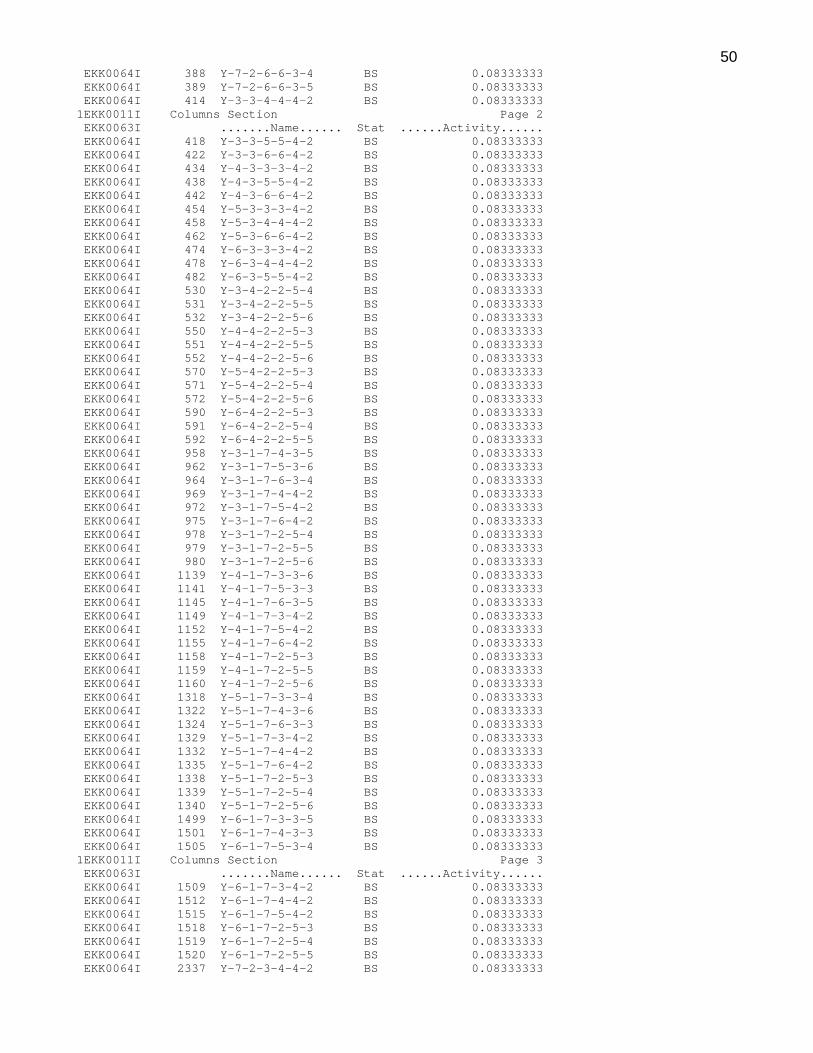
50 EKK0064I 388 Y-7-2-6-6-3-4 BS 0.08333333 EKK0064I 389 Y-7-2-6-6-3-5 BS 0.08333333 EKK0064I 414 Y-3-3-4-4-4-2 BS 0.08333333 1EKK0011I Columns Section Page 2 EKK0063I .......Name...... Stat ......Activity...... EKK0064I 418 Y-3-3-5-5-4-2 BS 0.08333333 EKK0064I 422 Y-3-3-6-6-4-2 BS 0.08333333 EKK0064I 434 Y-4-3-3-3-4-2 BS 0.08333333 EKK0064I 438 Y-4-3-5-5-4-2 BS 0.08333333 EKK0064I 442 Y-4-3-6-6-4-2 BS 0.08333333 EKK0064I 454 Y-5-3-3-3-4-2 BS 0.08333333 EKK0064I 458 Y-5-3-4-4-4-2 BS 0.08333333 EKK0064I 462 Y-5-3-6-6-4-2 BS 0.08333333 EKK0064I 474 Y-6-3-3-3-4-2 BS 0.08333333 EKK0064I 478 Y-6-3-4-4-4-2 BS 0.08333333 EKK0064I 482 Y-6-3-5-5-4-2 BS 0.08333333 EKK0064I 530 Y-3-4-2-2-5-4 BS 0.08333333 EKK0064I 531 Y-3-4-2-2-5-5 BS 0.08333333 EKK0064I 532 Y-3-4-2-2-5-6 BS 0.08333333 EKK0064I 550 Y-4-4-2-2-5-3 BS 0.08333333 EKK0064I 551 Y-4-4-2-2-5-5 BS 0.08333333 EKK0064I 552 Y-4-4-2-2-5-6 BS 0.08333333 EKK0064I 570 Y-5-4-2-2-5-3 BS 0.08333333 EKK0064I 571 Y-5-4-2-2-5-4 BS 0.08333333 EKK0064I 572 Y-5-4-2-2-5-6 BS 0.08333333 EKK0064I 590 Y-6-4-2-2-5-3 BS 0.08333333 EKK0064I 591 Y-6-4-2-2-5-4 BS 0.08333333 EKK0064I 592 Y-6-4-2-2-5-5 BS 0.08333333 EKK0064I 958 Y-3-1-7-4-3-5 BS 0.08333333 EKK0064I 962 Y-3-1-7-5-3-6 BS 0.08333333 EKK0064I 964 Y-3-1-7-6-3-4 BS 0.08333333 EKK0064I 969 Y-3-1-7-4-4-2 BS 0.08333333 EKK0064I 972 Y-3-1-7-5-4-2 BS 0.08333333 EKK0064I 975 Y-3-1-7-6-4-2 BS 0.08333333 EKK0064I 978 Y-3-1-7-2-5-4 BS 0.08333333 EKK0064I 979 Y-3-1-7-2-5-5 BS 0.08333333 EKK0064I 980 Y-3-1-7-2-5-6 BS 0.08333333 EKK0064I 1139 Y-4-1-7-3-3-6 BS 0.08333333 EKK0064I 1141 Y-4-1-7-5-3-3 BS 0.08333333 EKK0064I 1145 Y-4-1-7-6-3-5 BS 0.08333333 EKK0064I 1149 Y-4-1-7-3-4-2 BS 0.08333333 EKK0064I 1152 Y-4-1-7-5-4-2 BS 0.08333333 EKK0064I 1155 Y-4-1-7-6-4-2 BS 0.08333333 EKK0064I 1158 Y-4-1-7-2-5-3 BS 0.08333333 EKK0064I 1159 Y-4-1-7-2-5-5 BS 0.08333333 EKK0064I 1160 Y-4-1-7-2-5-6 BS 0.08333333 EKK0064I 1318 Y-5-1-7-3-3-4 BS 0.08333333 EKK0064I 1322 Y-5-1-7-4-3-6 BS 0.08333333 EKK0064I 1324 Y-5-1-7-6-3-3 BS 0.08333333 EKK0064I 1329 Y-5-1-7-3-4-2 BS 0.08333333 EKK0064I 1332 Y-5-1-7-4-4-2 BS 0.08333333 EKK0064I 1335 Y-5-1-7-6-4-2 BS 0.08333333 EKK0064I 1338 Y-5-1-7-2-5-3 BS 0.08333333 EKK0064I 1339 Y-5-1-7-2-5-4 BS 0.08333333 EKK0064I 1340 Y-5-1-7-2-5-6 BS 0.08333333 EKK0064I 1499 Y-6-1-7-3-3-5 BS 0.08333333 EKK0064I 1501 Y-6-1-7-4-3-3 BS 0.08333333 EKK0064I 1505 Y-6-1-7-5-3-4 BS 0.08333333 1EKK0011I Columns Section Page 3 EKK0063I .......Name...... Stat ......Activity...... EKK0064I 1509 Y-6-1-7-3-4-2 BS 0.08333333 EKK0064I 1512 Y-6-1-7-4-4-2 BS 0.08333333 EKK0064I 1515 Y-6-1-7-5-4-2 BS 0.08333333 EKK0064I 1518 Y-6-1-7-2-5-3 BS 0.08333333 EKK0064I 1519 Y-6-1-7-2-5-4 BS 0.08333333 EKK0064I 1520 Y-6-1-7-2-5-5 BS 0.08333333 EKK0064I 2337 Y-7-2-3-4-4-2 BS 0.08333333

51 EKK0064I 2340 Y-7-2-3-5-4-2 BS 0.08333333 EKK0064I 2343 Y-7-2-3-6-4-2 BS 0.08333333 EKK0064I 2346 Y-7-2-3-2-5-4 BS 0.08333333 EKK0064I 2347 Y-7-2-3-2-5-5 BS 0.08333333 EKK0064I 2348 Y-7-2-3-2-5-6 BS 0.08333333 EKK0064I 2361 Y-7-2-4-3-4-2 BS 0.08333333 EKK0064I 2364 Y-7-2-4-5-4-2 BS 0.08333333 EKK0064I 2367 Y-7-2-4-6-4-2 BS 0.08333333 EKK0064I 2370 Y-7-2-4-2-5-3 BS 0.08333333 EKK0064I 2371 Y-7-2-4-2-5-5 BS 0.08333333 EKK0064I 2372 Y-7-2-4-2-5-6 BS 0.08333333 EKK0064I 2385 Y-7-2-5-3-4-2 BS 0.08333333 EKK0064I 2388 Y-7-2-5-4-4-2 BS 0.08333333 EKK0064I 2391 Y-7-2-5-6-4-2 BS 0.08333333 EKK0064I 2394 Y-7-2-5-2-5-3 BS 0.08333333 EKK0064I 2395 Y-7-2-5-2-5-4 BS 0.08333333 EKK0064I 2396 Y-7-2-5-2-5-6 BS 0.08333333 EKK0064I 2409 Y-7-2-6-3-4-2 BS 0.08333333 EKK0064I 2412 Y-7-2-6-4-4-2 BS 0.08333333 EKK0064I 2415 Y-7-2-6-5-4-2 BS 0.08333333 EKK0064I 2418 Y-7-2-6-2-5-3 BS 0.08333333 EKK0064I 2419 Y-7-2-6-2-5-4 BS 0.08333333 EKK0064I 2420 Y-7-2-6-2-5-5 BS 0.08333333 EKK0064I 2503 Y-3-3-4-2-5-6 BS 0.08333333 EKK0064I 2514 Y-3-3-5-2-5-4 BS 0.08333333 EKK0064I 2527 Y-3-3-6-2-5-5 BS 0.08333333 EKK0064I 2562 Y-4-3-3-2-5-5 BS 0.08333333 EKK0064I 2575 Y-4-3-5-2-5-6 BS 0.08333333 EKK0064I 2586 Y-4-3-6-2-5-3 BS 0.08333333 EKK0064I 2623 Y-5-3-3-2-5-6 BS 0.08333333 EKK0064I 2634 Y-5-3-4-2-5-3 BS 0.08333333 EKK0064I 2647 Y-5-3-6-2-5-4 BS 0.08333333 EKK0064I 2682 Y-6-3-3-2-5-4 BS 0.08333333 EKK0064I 2695 Y-6-3-4-2-5-5 BS 0.08333333 EKK0064I 2706 Y-6-3-5-2-5-3 BS 0.08333333 EKK0064I 4367 Z(417723336) BS 0.08333333 EKK0064I 4372 Z(417723642) BS 0.08333333 EKK0064I 4375 Z(417723256) BS 0.08333333 EKK0064I 4381 Z(517723334) BS 0.08333333 EKK0064I 4385 Z(517723442) BS 0.08333333 EKK0064I 4389 Z(517723254) BS 0.08333333 EKK0064I 4397 Z(617723335) BS 0.08333333 EKK0064I 4402 Z(617723542) BS 0.08333333 EKK0064I 4405 Z(617723255) BS 0.08333333 EKK0064I 4426 Z(317724435) BS 0.08333333 EKK0064I 4430 Z(317724542) BS 0.08333333 1EKK0011I Columns Section Page 4 EKK0063I .......Name...... Stat ......Activity...... EKK0064I 4434 Z(317724255) BS 0.08333333 EKK0064I 4442 Z(517724436) BS 0.08333333 EKK0064I 4447 Z(517724642) BS 0.08333333 EKK0064I 4450 Z(517724256) BS 0.08333333 EKK0064I 4456 Z(617724433) BS 0.08333333 EKK0064I 4460 Z(617724342) BS 0.08333333 EKK0064I 4464 Z(617724253) BS 0.08333333 EKK0064I 4487 Z(317725536) BS 0.08333333 EKK0064I 4492 Z(317725642) BS 0.08333333 EKK0064I 4495 Z(317725256) BS 0.08333333 EKK0064I 4501 Z(417725533) BS 0.08333333 EKK0064I 4505 Z(417725342) BS 0.08333333 EKK0064I 4509 Z(417725253) BS 0.08333333 EKK0064I 4517 Z(617725534) BS 0.08333333 EKK0064I 4522 Z(617725442) BS 0.08333333 EKK0064I 4525 Z(617725254) BS 0.08333333 EKK0064I 4546 Z(317726634) BS 0.08333333 EKK0064I 4550 Z(317726442) BS 0.08333333 EKK0064I 4554 Z(317726254) BS 0.08333333

52 EKK0064I 4562 Z(417726635) BS 0.08333333 EKK0064I 4567 Z(417726542) BS 0.08333333 EKK0064I 4570 Z(417726255) BS 0.08333333 EKK0064I 4576 Z(517726633) BS 0.08333333 EKK0064I 4580 Z(517726342) BS 0.08333333 EKK0064I 4584 Z(517726253) BS 0.08333333 EKK0064I 5121 Z(723334442) BS 0.08333333 EKK0064I 5125 Z(723334256) BS 0.08333333 EKK0064I 5150 Z(517334442) BS 0.08333333 EKK0064I 5152 Z(517334256) BS 0.08333333 EKK0064I 5205 Z(723335542) BS 0.08333333 EKK0064I 5208 Z(723335254) BS 0.08333333 EKK0064I 5246 Z(617335542) BS 0.08333333 EKK0064I 5248 Z(617335254) BS 0.08333333 EKK0064I 5289 Z(723336642) BS 0.08333333 EKK0064I 5293 Z(723336255) BS 0.08333333 EKK0064I 5318 Z(417336642) BS 0.08333333 EKK0064I 5320 Z(417336255) BS 0.08333333 EKK0064I 5541 Z(724433342) BS 0.08333333 EKK0064I 5544 Z(724433255) BS 0.08333333 EKK0064I 5582 Z(617433342) BS 0.08333333 EKK0064I 5584 Z(617433255) BS 0.08333333 EKK0064I 5625 Z(724435542) BS 0.08333333 EKK0064I 5629 Z(724435256) BS 0.08333333 EKK0064I 5654 Z(317435542) BS 0.08333333 EKK0064I 5656 Z(317435256) BS 0.08333333 EKK0064I 5709 Z(724436642) BS 0.08333333 EKK0064I 5712 Z(724436253) BS 0.08333333 EKK0064I 5750 Z(517436642) BS 0.08333333 EKK0064I 5752 Z(517436253) BS 0.08333333 EKK0064I 5961 Z(725533342) BS 0.08333333 EKK0064I 5965 Z(725533256) BS 0.08333333 EKK0064I 5990 Z(417533342) BS 0.08333333 EKK0064I 5992 Z(417533256) BS 0.08333333 1EKK0011I Columns Section Page 5 EKK0063I .......Name...... Stat ......Activity...... EKK0064I 6045 Z(725534442) BS 0.08333333 EKK0064I 6048 Z(725534253) BS 0.08333333 EKK0064I 6086 Z(617534442) BS 0.08333333 EKK0064I 6088 Z(617534253) BS 0.08333333 EKK0064I 6129 Z(725536642) BS 0.08333333 EKK0064I 6133 Z(725536254) BS 0.08333333 EKK0064I 6158 Z(317536642) BS 0.08333333 EKK0064I 6160 Z(317536254) BS 0.08333333 EKK0064I 6381 Z(726633342) BS 0.08333333 EKK0064I 6384 Z(726633254) BS 0.08333333 EKK0064I 6422 Z(517633342) BS 0.08333333 EKK0064I 6424 Z(517633254) BS 0.08333333 EKK0064I 6465 Z(726634442) BS 0.08333333 EKK0064I 6469 Z(726634255) BS 0.08333333 EKK0064I 6494 Z(317634442) BS 0.08333333 EKK0064I 6496 Z(317634255) BS 0.08333333 EKK0064I 6549 Z(726635542) BS 0.08333333 EKK0064I 6552 Z(726635253) BS 0.08333333 EKK0064I 6590 Z(417635542) BS 0.08333333 EKK0064I 6592 Z(417635253) BS 0.08333333 EKK0064I 7410 Z(433342255) BS 0.08333333 EKK0064I 7414 Z(533342256) BS 0.08333333 EKK0064I 7416 Z(633342254) BS 0.08333333 EKK0064I 7427 Z(417342256) BS 0.08333333 EKK0064I 7432 Z(517342254) BS 0.08333333 EKK0064I 7439 Z(617342255) BS 0.08333333 EKK0064I 7465 Z(724342256) BS 0.08333333 EKK0064I 7466 Z(725342254) BS 0.08333333 EKK0064I 7469 Z(726342255) BS 0.08333333 EKK0064I 7711 Z(334442256) BS 0.08333333 EKK0064I 7713 Z(534442253) BS 0.08333333

53 EKK0064I 7717 Z(634442255) BS 0.08333333 EKK0064I 7726 Z(317442255) BS 0.08333333 EKK0064I 7733 Z(517442256) BS 0.08333333 EKK0064I 7738 Z(617442253) BS 0.08333333 EKK0064I 7764 Z(723442255) BS 0.08333333 EKK0064I 7767 Z(725442256) BS 0.08333333 EKK0064I 7768 Z(726442253) BS 0.08333333 EKK0064I 8010 Z(335542254) BS 0.08333333 EKK0064I 8014 Z(435542256) BS 0.08333333 EKK0064I 8016 Z(635542253) BS 0.08333333 EKK0064I 8027 Z(317542256) BS 0.08333333 EKK0064I 8032 Z(417542253) BS 0.08333333 EKK0064I 8039 Z(617542254) BS 0.08333333 EKK0064I 8065 Z(723542256) BS 0.08333333 EKK0064I 8066 Z(724542253) BS 0.08333333 EKK0064I 8069 Z(726542254) BS 0.08333333 EKK0064I 8311 Z(336642255) BS 0.08333333 EKK0064I 8313 Z(436642253) BS 0.08333333 EKK0064I 8317 Z(536642254) BS 0.08333333 EKK0064I 8326 Z(317642254) BS 0.08333333 EKK0064I 8333 Z(417642255) BS 0.08333333 EKK0064I 8338 Z(517642253) BS 0.08333333 1EKK0011I Columns Section Page 6 EKK0063I .......Name...... Stat ......Activity...... EKK0064I 8364 Z(723642254) BS 0.08333333 EKK0064I 8367 Z(724642255) BS 0.08333333 EKK0064I 8368 Z(725642253) BS 0.08333333 EKK0317I Entering OSL module ekk_deleteModel (xtsp73)

54Appendix E:
Summary of the TSP Tours Comprising the
Solution for the Dual Form of Problem xtsp73

55
Tour # Sequence “Weight” (Flow Value)
1 1-5-7-3-4-2-6-1 0.083333
2 1-5-7-4-6-2-3-1 0.083333
3 1-5-7-6-3-2-4-1 0.083333
4 1-6-7-3-5-2-4-1 0.083333
5 1-6-7-4-3-2-5-1 0.083333
6 1-6-7-5-4-2-3-1 0.083333
7 1-3-7-4-5-2-6-1 0.083333
8 1-3-7-5-6-2-4-1 0.083333
9 1-3-7-6-4-2-5-1 0.083333
10 1-4-7-3-6-2-5-1 0.083333
11 1-4-7-5-3-2-6-1 0.083333
12 1-4-7-6-5-2-3-1 0.083333
Table E.1: Summary of the TSP tours in the Solution
to Problem xtsp73 Using the Dual Form