P r a c t ic a l s - scienceandmathsrevision.co.uk

MODULE 1

Practicals This guide goes through each of the practicals, outlining the methods and any analysis or evaluation which will be helpful.

Determining g There are two experiments used to find the value of g which you will need to know. Trap door and electromagnet method: Apparatus required:

● Electromagnet ● Steel ball ● Trap door ● Timer circuit ● Ruler

Method: 1. Set up apparatus so the ball is just held up by the electromagnet -

measure the distance from electromagnet to trapdoor 2. Switch off electromagnet, this starts the timer and releases the ball 3. When the ball hits the trapdoor, the timer is stopped 4. Change height of ball and test for a range of different heights

Analysis and evaluation: ● Produce a graph of distance against time squared (as , )t ats = u + 2

1 2 so s atu = 0 = 21 2

● The gradient is half of g ( )g =t22s

● If current too high, the ball will release after delay, make sure ball only just held ● If the distance to fall is too great, air resistance might have a big impact on the result ● Measurement of distance will be another source of uncertainty

Light gate method: Apparatus:

● Card ● Light gate ● Data logger ● Ruler

Method: 1. Drop the card vertically through the light gate, measuring the distance it is above the light gate and the length of

the card 2. The light gate measures the velocity of the card 3. Vary the height at which the card is dropped from

Analysis and evaluation: ● Plot a graph of against s ( , u is 0 so )v2 asv2 = u2 + 2 asv2 = 2 ● Gradient is equal to 2g as g = 2s

v2

● The method assumes velocity of the card will be constant as it passes through gate, measure the height from the centre of the card to reduce the error

Determining terminal velocity An experiment can be carried out in a lab to calculate the terminal velocity of a mass as it falls through a fluid. Liquids which are ideal include heavy oil and wallpaper paste - as they are denser making the object fall slower and therefore makes determining speeds easier. Equipment required: ball bearing, cylinder, clamps, elastic band, viscous liquid, stop watch, metre rule

Made by Sophie Drew for www.scienceandmathsrevision.co.uk

MODULE 1 Brief method:

● Set up a clamped cylinder filled with the liquid ● Drop the ball bearing into the liquid and start the stopwatch ● At set time periods put elastic bands onto the cylinder at the place where the ball is ● When the ball reaches the bottom, measure the distance between each elastic band ● Using the time period, find the velocity in between each section ● Plot a graph of velocity against time, they will be joined with as smooth curve, the

point where the gradient is 0 will be the terminal velocity Improvements:

● Attach ball to ticker tape which punches holes at a set time interval and use the distance between the dots to find the velocities

● Use a more viscous fluid to slow the ball more, improving accuracy of placement of bands

Investigating force-extension characteristics In the lab you can investigate the force-extension characteristics of different materials. The experiment is outlined below:

● The material will be suspended using a clamp stand, clamp and boss ● A ruler will be placed alongside, with a ficidual marker showing the original length ● A range of masses are placed onto the spring and a measurement of extension is made ● Analyse the results by plotting graphs of force against extension ● The force constant can be found by finding the gradient of the graph before the elastic limit is reached (this part of

the graph will be a straight line)

Determining Young modulus The Young modulus of a metal can be found using the following procedure:

● Measure the diameter of the wire using a micrometer (measure at a range of places to determine an average) then use this to find the cross-sectional area

● Clamp the wire at one end and attach to a pulley on the other - measure the length with a meter rule ● Place a ruler parallel to the wire and attach a ficidual mark ● Apply different forces to the wire using masses at the end, measure the extension using the ficidual mark to help ● Calculate the stress and strain from the results and plot a stress-strain graph. The Young-modulus will be the

gradient of this graph. Investigating electrical characteristics of ohmic and non-ohmic conductors The following experiment can be done to investigate I-V characteristics of different components:

● Set up a circuit containing a variable power supply, ammeter, voltmeter and component testing ● Take readings for the current and potential difference as the voltage of the power supply is changed ● Use these readings to plot an I-V graph for the component

Determining resistivity You can determine the resistivity of a wire by finding the current and pd for different lengths of wire. This experiment is outlined below:

● Set up a circuit with the wire and a battery. Use an ammeter and voltmeter to find the current and voltage. A variable resistor is also used to ensure the current is kept low - this reduces errors from heating effect

● Take readings for voltage and current for a range of lengths and use them to find resistance

● Measure the diameter of the wire using a micrometer - measure in more than one place as the wire may not be perfectly cylindrical. Use this to find cross-sectional area


MODULE 1

● Plot R against l and find the gradient, this gives . The graph should be a straight linelR

● As resistivity is , multiply the gradient by the cross section to find resistivitylRA

Determining internal resistance An experiment can be carried out in order to determine the internal resistance of a cell. The procedure is described below:

● Connect the cell in series with a variable resistor ● Measure the current through the circuit and the terminal pd as you adjust the variable resistor ● Plot a graph of V against I - it should produce a straight line

○ We can rearrange the equation to rε = V + I − rV = I + ε ○ Thinking of this in the form , we see that -r is the gradient and is the y-interceptxy = m + c ε

● Find the gradient of the line to determine the internal resistance. Investigating potential dividers An investigation of potential divider circuits can be carried out to find how the changes in different conditions.V out

● Start by setting up a potential divider circuit containing either a thermistor or an LDR, with a voltmeter across this component.

● For a thermistor circuit, alter the conditions using a water bath at different temperatures. Make readings for the output voltages at each temperature

● For an LDR circuit, place a bulb at a set distance away in a dark room. Alter the brightness (or distance) of the bulb and take readings for the voltage for each set up.

● You can then plot a graph to show the variation of voltage with changing condition.

Using oscilloscopes You can use an oscilloscope to find properties of waves, such as their frequency.

● A wave is produced by a signal generator or a microphone which is plugged into the oscilloscope ● The oscilloscope produces a graphical depiction of the wave with displacement on the y-axis and time along the x ● You will need to work out the timebase of the oscilloscope (usually labelled on axis), from this you can find the

period of the wave ● You can then find the frequency using the equation f = 1

T Demonstrate wave effects with ripple tank

● A ripple tank produces water waves with an oscillating paddle disturbing the water ● A light is shone above the waves and a screen below the tank shows the waves produced

○ Bright bands are crests ○ Dark bands are troughs ○ The wavelength is found by finding the distance between two crests

● A glass sheet can be placed in the water, changing its depth. ○ This demonstrates refraction as depth alters its speed ○ Measure the wavelength, if the wavelength has decreased the waves are slower

● Diffraction can be demonstrated by placing an obstacle in the water. If the gap as altered to be similar size to the wavelength, more diffraction occurs

Polarising effects of microwaves and light Polarising light:

● Polarisation of light can be demonstrated using two polarising filters ● Place them together at an angle of , no light will pass through90° ● Rotate by and the light intensity will increase to a maximum90° ● This demonstrates Malus’ law:

○ When the angle is , will be zero so the intensity is 090° θcos2 ○ When the angle is , will be 1, the maximum value it can take so the intensity is at a maximum0° θcos2

Polarising microwaves:


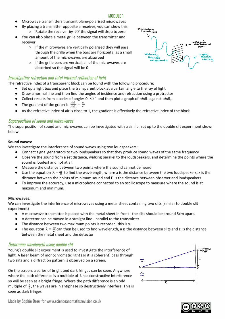
MODULE 1 ● Microwave transmitters transmit plane-polarised microwaves ● By placing a transmitter opposite a receiver, you can show this:

○ Rotate the receiver by the signal will drop to zero90° ● You can also place a metal grille between the transmitter and

receiver. ○ If the microwaves are vertically polarised they will pass

through the grille when the bars are horizontal as a small amount of the microwaves are absorbed

○ If the grille bars are vertical, all of the microwaves are absorbed so the signal will be 0

Investigating refraction and total internal reflection of light The refractive index of a transparent block can be found with the following procedure:

● Set up a light box and place the transparent block at a certain angle to the ray of light ● Draw a normal line and then find the angles of incidence and refraction using a protractor ● Collect results from a series of angles 0- and then plot a graph of against 0 8 ° inθs 1 inθs 2

● The gradient of the graph is sinθ2

sinθ1 = n1

n2

● As the refractive index of air is close to 1, the gradient is effectively the refractive index of the block. Superposition of sound and microwaves The superposition of sound and microwaves can be investigated with a similar set up to the double slit experiment shown below. Sound waves: We can investigate the interference of sound waves using two loudspeakers:

● Connect signal generators to two loudspeakers so that they produce sound waves of the same frequency ● Observe the sound from a set distance, walking parallel to the loudspeakers, and determine the points where the

sound is loudest and not at all. ● Measure the distance between two points where the sound cannot be heard. ● Use the equation to find the wavelength, where a is the distance between the two loudspeakers, x is theλ = D

ax distance between the points of minimum sound and D is the distance between observer and loudspeakers.

● To improve the accuracy, use a microphone connected to an oscilloscope to measure where the sound is at maximum and minimum.

Microwaves: We can investigate the interference of microwaves using a metal sheet containing two slits (similar to double slit experiment)

● A microwave transmitter is placed with the metal sheet in front - the slits should be around 5cm apart. ● A detector can be moved in a straight line - parallel to the transmitter. ● The distance between two maximum points is recorded, this is x. ● The equation can then be used to find wavelength, a is the distance between slits and D is the distanceλ = D

ax between the metal sheet and the detector

Determine wavelength using double slit Young’s double slit experiment is used to investigate the interference of light. A laser beam of monochromatic light (so it is coherent) pass through two slits and a diffraction pattern is observed on a screen. On the screen, a series of bright and dark fringes can be seen. Anywhere where the path difference is a multiple of has constructive interferenceλ so will be seen as a bright fringe. Where the path difference is an odd multiple of , the waves are in antiphase so destructively interfere. This is2

λ seen as dark fringes.


MODULE 1 From this experiment, you can calculate the wavelength of the light from the laser. The formula is:

λ = Dax

Where is wavelength, is the separation between the two slits, is the separation between two bright fringes and isλ a x D the distance between the screen and the slits.

Determine wavelength with diffraction grating A diffraction grating can be used to find the wavelength of light. The method is outlined below:

● A diffraction grating is put in front of a beam of monochromatic light ● A series of dark and bright fringes appear on the screen ● The spacing between the slits can be found with the following equation: where x is the number of slits perd = x

1 metre

● The angle theta is found either using a protractor or finding the distance between two fringes and the total distance to the screen then using trigonometry

● The equation can then be used to find the wavelengthλ sinθn = d

Using LEDs to find Planck constant An experiment using LEDs can be used to calculate the value of Planck’s constant. LEDs come in many different colours and each of these colours are linked to a specific wavelength which we know. We can use the activation voltages to determine planck’s constant. The method is outlined below:

● Set up the circuit as shown below:

● Measure the current as the voltage is changed by altering the variable resistor. ● Plot a graph of current against pd for each LED ● The activation voltage is the point where the current starts to increase linearly (this can also be determined by

finding the voltage when the LED turns on - but this is less accurate) ● Plot a graph of activation voltage against 1 over wavelength:

● The photon energy is equal to the energy of the electrons going through the LED (eV), so: ○ Ve = λ

hc ○ This is rearranged to:V = e

hcλ1

○ Compare this with , the gradient is xy = m + c ehc

● Find the gradient of the line and multiply by (a constant) to find Planck’s constant.ce


MODULE 1 Demonstrate photoelectric effect The photoelectric effect can be observed using a gold-leaf electroscope, shown below: The metal plate is negatively charged, making the stem and leaf also negative - they repel and the leaf moves away. When visible light is incident on the plate, nothing happens. However, when UV light is incident, the leaf moves back in, the charge is reduced. This is due to the photoelectric effect, UV light has high enough photon energy to remove electrons from the metal surface, thus reducing the charge on the stem and leaf. Determine SHC of metal electrically The specific heat capacity of a material can be found electronically, using an immersion heater. The methods for determining SHC for a solid and a liquid are very similar but with slight differences in set up.

● Measure the mass of the substance that you are finding the SHC of ● The material is placed inside an insulating material, for a liquid

also use a lid ● An immersion heater is placed into the material along with a

thermometer, record the starting temperature ● Turn on the immersion heater and take readings for the current

and pd using an ammeter and voltmeter ● Start the timer and, after a set time, take a reading for the final

temperature ● Use the equation to find the electrical energy suppliedItE = V ● Use the equation and rearrange it to cΔθE = m c = E

mΔθ ● Substitute in values of E,m and to find the specific heat capacityθ

of the substance Determine SLH Specific latent heat of fusion: This experiment determines the specific latent heat of fusion for ice as it changes to water:

● Start by setting up the equipment, place the ice into a funnel above a beaker. Place the electric heater into the ice. Set up two of these arrangements

● Connect one of the heaters to a power supply in a circuit containing an ammeter and voltmeter and leave the other one, this is the control

● Turn the heater on for 15 minutes and record the current and voltage in the circuit.


MODULE 1 ● Measure the mass of water in the two beakers at the end, the difference in these masses will be the ice melted due

to the heater ● Find the energy supplied to the heater using and then divide by mass to find the specific latent heatItE = V

Specific latent heat of vaporisation: This experiment determines the specific latent heat of vaporisation of a liquid:

● Set up the equipment as in the diagram shows ● Heat the liquid with a heater, measuring the pd and current using an ammeter and

a voltmeter ● When the liquid boils, the vapour passes out into the condenser and collects in a

beaker below ● Over a certain time, measure the mass collected in the beaker. ● Using the latent heat equation, we produce the equation I t LV 1 1 = m1 + Q

○ Q is the energy wasted as heat ○ is the energy suppliedI tV 1 1

● Repeat the experiment but use a different pd and current but same time period ● The equation for this experiment will be I t LV 2 2 = m2 + Q ● By subtracting one equation from the other, we can remove the unknown Q, this

leaves: ○ V I I )t m )L( 2 2 − V 1 1 = ( 2 − m1 ○ We know all of these values except L, so can rearrange to find the specific latent heat of vaporisation.

Investigating circular motion with whirling bung Circular motion can be investigated using a whirling bung. The experiment is outlined below:

● Tie a bung to one end of the string ● Attach a 1N weight to the other side of the string, a set distance apart ● Rotate the bung (with a fixed radius) and adjust the speed so that the radius stays constant. ● Time how long it takes to do ten rotations ● Use this, along with the radius, in order to calculate speed of rotation ● Repeat this method with a range of forces and then plot a graph of F against v2

Determine period and frequency of SHM We can carry out an experiment to investigate how different factors will affect the frequency/period of oscillations, the experiment below can use a pendulum or a spring

● Start by setting up equipment as shown in the diagrams below:

● A stopwatch can be used to determine how long it takes for 10 oscillations (lower percentage uncertainty than one

oscillation) ● Use a fiducial marker to improve accuracy here. A plumb line can be used for a pendulum and the oscillation

starting and ending as it crosses this. For a spring you can use a ruler in a background and start and stop the timer at a certain point.

● The period can then be found for a single oscillation by dividing the time by 10. The reciprocal of the period gives frequency

● Changing either the mass or the amplitude of oscillations for each experiment can be used to investigate how these factors affect the frequency of oscillation.


MODULE 1 Investigating capacitors in series and parallel We can investigate the capacitance of capacitors in series and parallel to check that these rules work. The method for this is outlined below:

● Start by setting up the circuit as in the diagram below - putting the chosen combination of capacitors where the capacitor is shown

● Close the switch and use the variable resistor to keep the current constant. ● At the same time as closing the switch, start the timer ● Record values for current and pd until there is no longer a current flowing - the capacitors are now fully charged ● Use the equation to find the charge stored by the capacitors.tQ = I

● We can now calculate the capacitance of the combination using: C = QV

● The measured values of capacitance can be compared to the calculated ones Investigating charge and discharge of capacitors An experiment can be carried out to investigate how the potential difference and current change as capacitors charge and discharge. The method is given below:

● A circuit is set up as shown below, using a capacitor with high capacitance and a resistor of high resistance slows down the changes (higher time constant) so it is easier to measure:

● The switch is closed at A and the capacitor begins to charge ● Record the current and pd every 20 seconds ● Once the capacitor is fully charged, close the switch at B and measure the current and pd every 20 seconds. ● Plot graphs for the current and pd as the capacitor is first charged then discharged.

Determining flux density using balance An experiment can be used to find the flux density of a magnetic field between two poles of a magnet, by measuring the force experienced by a wire in the field. The experiment is outlined below:

● The equipment is set up as shown to the right, with the magnets on the balance and the wires above, not touching it.

● Supply is turned on and the current measured. A force is exerted on the wire, it will exert an equal and opposite force on the magnet.

● The force on the magnet will change the weight. We can record the change in mass and calculate the force with gF = m

● We know that and when so we can use ILsinθF = B inθs = 1 0θ = 9 ILF = B ● Measure the length of the wire ● Rearrange the equation for B: and use it to calculate the flux density.B = F

IL


MODULE 1 Investigating transformers We can carry out an experiment to investigate how the change in the turns will affect the emf in the primary and secondary coils, this experiment is outlined below:

● Wrap two coils around an iron bar, each with 30 coils. Attach the primary coil to a power supply and a voltmeter in parallel. Connect the secondary coil to a voltmeter.

● Record the primary and secondary voltages. ● Keep the number of coils on the primary coil the same, but alter the coils on the secondary coil. ● Plot a graph to show that the equation is true.np

ns = V sV p

Investigating absorption of radiation An experiment can be carried out to investigate which materials will absorb the different types of radiation. The method is outlined below:

● First measure the background radiation using the Geiger-Muller tube and record the count rate ● The activity of a radioactive source emitting alpha radiation is measured with a Geiger-Muller tube ● The initial count rate is recorded ● Different materials are placed between the source and the tube - paper, aluminium and then lead. Record the

count rate for each of the materials ● Repeat for a Beta and then a Gamma source ● Subtract the background count rate from all the results and then use the final results to determine which type of

radiation was stopped by each material Determining half-life of isotopes We can experimentally determine the half-life of a radioactive isotope such as protactinium. The method is outlined below:

● A bottle containing uranium salt solution and protactinium in an immiscible layer of solvent is used ● The bottle is shaken and the protactinium-234 is dissolved into the other layer ● Start by measuring the background radiation with the Geiger-Muller tube ● The beta decay of the protactinium is measured with a Geiger-Muller tube connected to a data-logger ● The uranium sample also decays but releases alpha radiation, which is absorbed by the bottle ● The activity is monitored against time, allowing the half-life to be determined - make sure the background activity

is subtracted from the activity first. Modelling radioactive decay Radioactive decay can be modelled using a spreadsheet or with dice. The two investigations are described below: Spreadsheet: We can model decay using the equation . We can set up a spreadsheet to complete multiple iterations to model− NΔt

ΔN = λ decay:

● Lay out four columns, titled: time, number of nuclei, number of decays and new nuclei: ● We know that number of decays can be found using: N − N tΔ = λ × Δ ● Set this as the formula for number of decays in that column, make tΔ = 1 ● In the time column put the numbers 0-100 increasing by 1 each time ● Now write new nuclei to be , this can then be put into the number of nuclei cell in the row belowNN − Δ ● Put in a start number of nuclei and the spreadsheet will model decay

Dice: We can simulate radioactive decay with dice, a large number of dice is required for the model to work. Each dice represents an undecayed nucleus and when a 6 is throw it is said to have decayed:

● Roll all of the dice ● Remove any which roll a 6, record the new number of dice remaining ● Continue to record the number of dice and those removed for each roll ● Repeat until there are no dice left


MODULE 1 ● Use the data to determine the half-life and the decay constant ● As the decay constant is the probability of an individual nucleus decaying, we would expect it to be as this is the6

1 probability of the dice ‘decaying’ by rolling a 6

● By using dice with a different number of sides or by allowing more than one number to result in decay, the simulation can be repeated for an isotope with a different half-life.


Documents

P r a c t ic a l s - scienceandmathsrevision.co.uk