Embed Size (px)
Citation preview

OSHPC BARKI TOJIK
TECHNO-ECONOMIC ASSESSMENT STUDY FOR ROGUN HYDROELECTRIC CONSTRUCTION PROJECT
HYDROLOGY
JANUARY 2013

TEAS for Rogun HPP Construction Project
Hydrology - January 2013
TECHNO-ECONOMIC ASSESSMENT STUDY FOR ROGUN HYDROELECTRIC CONSTRUCTION PROJECT
HYDROLOGY
JANUARY 2013
Report No. P.002378 RP 07 rev.D
D 15/01/2013 Draft Version for Disclosure H. GARROS NSA NSA
C 07/01/2013 Final H. GARROS ALA NSA
B 10/08/2012 Rev B H. GARROS R. ALBERT NSA
A 11/07/2011 First Draft H.GARROS R.ALBERT R ALBERT
Revision Date Subject of revision Drafted Checked Approved

TEAS for Rogun HPP Construction Project
Hydrology - January 2013
January 2013 3/104
Table of Content
Table of Content 3
References 5
Notations 6
List of Tables 8
1. INTRODUCTION 9
2. GENERAL SITUATION 9
2.1 Geography 9
2.2 Hydrological regime 10
2.3 hydrometeorologic data 13
2.4 Climatic data 13
2.5 Hydrometric data 14
3. INFLOWS 15
3.1 Inflows assessment 15
3.2 Yearly and Seasonal Inflows 15
3.3 Monthly Inflows 19
4. FLOODS 20
4.1 Data for Flood Study 20
4.2 Regional flood samples – General Approach 20
4.3 Regional Approach 22
4.3.1. First Step – Vakhsh River Basin 28
4.3.2. Second Step – Vakhsh River + Indus River + Chenab River 34
4.3.3. Third Step – Second Step + Syr Darya River 38
4.3.4. Flood Frequency and Flood Hydrographs 41
4.4 PMF Computation 44
4.4.1. Probable Maximum Flood (PMF) assessment 44
4.4.2. PMF According to 2006 study 46
4.4.3. Degree-Day Approach 48

TEAS for Rogun HPP Construction Project
Hydrology - January 2013
January 2013 4/104
4.4.4. Maximisation Procedures to Obtain PMF 52
4.4.5. First Maximisation: 55
4.4.6. Second Maximisation: 58
4.4.7. Third Maximisation: 60
4.4.8. PMF Choice and PMF Hydrograph 63
5. CLIMATE CHANGE 65
5.1 Data for Climate Change Analysis 66
5.2 Trend Analysis of Precipitation, Temperature and Discharge 66
5.2.1 Trend Analysis of Precipitation 66
5.2.2 Trend Analysis of Temperature 72
5.2.3 Trend Analysis of Discharges 76
5.2.4 Existing models in Central Asia – Temperature and Precipitation Projections 81
5.3 Snow Accumulation and Glacier Melt 83
5.3.1. Analysis of Regional Information 83
5.3.2. Analysis of Tajikistan and Vakhsh Contexts 88
5.3.3. Scenario 1: Impacts of Glacier Disappearance 95
5.4 Scenario 2: Evolution of Discharges from 1990 to 21 00 99
5.5 Climate Change and Adaptive Management: 103
5.5.1. Climate Change models as a tool to set up priorities: 103
5.5.2. Adaptation measures to Climate Change: 104

TEAS for Rogun HPP Construction Project
Hydrology - January 2013
January 2013 5/104
References
Author(s) Date Title
Palgov, N. N. 1947Relationship between air temperature and melting of glaciers in Zailiyskiy Alateau. Vestnik of Academy of Science of Kazakhstan SSR, n°10(10).
Shults, V. 1958 Hydrography of Central Asia. Tashkent: CAGU publishers.
Krenke, A. N., & Khodakov, V. G. 1966Relationship between glacier surface melting and air temperature. Materials of glacier studies, chronicles of discussions n°12.
Tronov, M. V. 1966 Glaciers and climate. L. Gidrometeoizdat.
Francou, J., & Rodier, J. 1967Essai de classification des crues maximales observées dans le monde. Cahier O.R.S.T.O.M. série hydrologie, Vol IV n°3.
UNESCO 1976 World Catalogue of Very Large Floods.Krenke, A. N. 1982 Mass exchange in glacier systems in the USSR territory. L. Gidrometeoizdat.Rodier, J. A., & Roche M. 1984 World Catalogue of Maximum Obseved Floods. IAHS Publication n°143.WMO 1986 Manual for Estimation of Probable Maximum Precipitation.World Meteorological Organisation 1986 Intercomparison of models of snowmelt runoff, report n°23. Genève.Hydrometheoizdat, L. 1988 Applied scientific Reference Book on Climate of the USSR, issue 31.
Garros-Berthet, H 1994Station‐Year Approach: A Tool for Estimation of Design Floods.Journal of Water Resources Planning and Management 120(2), 135–160.
Kuchment L.S. 1997Estimating the risk of rainfall and snowmelt disastrous floods using physically-based models of river runoff generation.
Garros-Berthet, H. 1998Station-year and Lombardi's approach: tools for estimation of design floods. ICOLD Barcelona Symposium on Dam Safety. Barcelona.
Gibb and al. 2000 Nurek Dam - Safety Assessment Refort.
Ohmura, A. 2001Physical basis for the temperature-based melt method. Journal of Applied Meteorology, 40(4), 753-761.
Makhmadaliev, Novikov and al. 2002The First National Communication of the Republic of Tajikistan on the UN Framework Convention on Climate Change.
Makhmadaliev, Novikov and al. 2003The First National Communication of the Republic of Tajikistan on the UN Framework Convention on Climate Change. Phase 2. Capacity Building in Priority Areas.
Savoskul 2003 Water, Climate, Food and Environment in the Syr Darya Basin.
Homidov A. 2006Field Research of glaciers and glacial lakes located in Karatag, VakhshAnd Zeravshan river basins.
Lahmeyer 2006 Volume 3 D - Hydrology.Christensen and al. 2007 Climate Change 2007 - Chapter 11 - Regional Climate Projections.Perelet 2007 Central Asia: Background Paper on Climate Change.
Makhmadaliev, Novikov and al. 2008The Second National Communication of the Republic of Tajikistan on the UN Framework Convention on Climate Change.
Hydroproject 2009 Final Design - Hydrometeorological Conditions.
Roy 2009Potential impacts of Climate Change on the hydrological regime of Tajikistan and the Kyrgyz Republic at the horizons 2050 and 2080.
World Meteorological Organisation. 2009 Manual on Estimation of Probable Maximum Precipitation, WMO n°1045. Geneva.
Siegfried and al. 2010 Will Climate Change Exacerbate or Mitigate Water Stress in Central Asia?
Siegfred and al. 2010Coping with International Water Confloct in Central Asia: Implications of Climate Change and Melting Ice in the Syr Darya Catchment.
Yasinkiy V.A, Mironenkov A.P, Sarsembekov T.T 2012Priorities for cooperation in transboundary river basins in Central Asia - Eurasian Development Bank - Almaty

TEAS for Rogun HPP Construction Project
Hydrology - January 2013
January 2013 6/104
Notations
A Catchment area (km2).
Cv Coefficient of variation (Cv = S/M).
DDF Degree-Day factor (°C)
F Frequency.
K(Qp) Francou-Rodier’s Flood Rating. (Q/106) = (A/109)(1-01.K).
M Average of sampled data.
Max Maximum of sampled data.
Me Median of sampled data.
Min Minimum of sampled data.
n Sample size.
PMP Probable Maximum Precipitation (mm).
PMF Probable Maximum Flood (m3/s).
P(Oct/May) Seasonal Precipitation form October to May (mm).
Pyr Yearly precipitation (mm).
Q Discharge (m3/s).
Qd Daily discharge (m3/s).
Qdmx Maximum daily discharge (m3/s).
Qp Instantaneous peak discharge (m3/s).
QFit Fitted discharge (m3/s).
r Coefficient of correlation.
r2 Coefficient of determination.
RF Daily rainfall (mm).
RH Relative humidity (%).
RO Runoff (mm).
RO Flood runoff, (mm).
S Standard deviation of sampled data
T Return Period (years).

TEAS for Rogun HPP Construction Project
Hydrology - January 2013
January 2013 7/104
V Volume (Mm3).
Vyr Yearly inflow (Mm3).
Z Elevation (m).

TEAS for Rogun HPP Construction Project
Hydrology - January 2013
January 2013 8/104
List of Tables
Table 1: Gauging stations in the Vakhsh River Basin ................................................................... 14
Table 2:Data about Yearly and Seasonal Inflows at Rogun Damsite ........................................... 16
Table 3: Statistical parameters of monthly, yearly and seasonal inflows series 1932/2008: ........ 19
Table 4: Analogies between Regional River Basins ..................................................................... 23
Table 5: Cluster analysis of considered series of data .................................................................. 26
Table 6: First Step Regional Analysis ........................................................................................... 30
Table 7: Step 2 - Regional Sample of Flood Peaks at Rogun ...................................................... 35
Table 8: Step 3 - Regional Flood Sample at Rogun (287 Station-Years) ..................................... 39
Table 9: Rogun – Flood Frequency and Flood Hydrographs ........................................................ 42
Table 10: PMF Computation According to 2006 Study ................................................................. 47
Table 11: Second Maximisation - Using 40 Flood Events............................................................. 58
Table 12:Third Maximisation - Station Year Approach .................................................................. 61
Table 13: PMF Choice and PMF Hydrograph ............................................................................... 64
Table 14: Trend Analysis of Precipitation Data ............................................................................. 67
Table 15: Trend Analysis of Temperature Data ............................................................................ 73
Table 16: Trend Analysis of Discharges........................................................................................ 77
Table 17: Climate Change in Central Asia - Temperature and Precipitation ................................ 82
Table 18: Regional Information About Climate Change and Melt ................................................. 85
Table 19: Tajikistan and Vakhsh Contexts .................................................................................... 90
Table 20: Maximum Impact of Glacier Disappearance ................................................................. 95
Table 21: Evolution of Discharges from 1990 to 2100 ................................................................ 100
List of Figures Figure 2-1: Hydro meteorological network of the Vakhsh Basin, source Lahmeyer 2006 ............ 11
Figure 2-2 : Annual pattern of runoff at Rogun, and average precipitations and temperatures recorded at Obigam ....................................................................................................................... 12
Figure 2-3: Hydrographic network and hydrometeorological coverage of the Vakhsh River basin at the stretch between Rogun Dam Site and Sangtuda, source Lahmeyer 2006 ........................ 13

TEAS for Rogun HPP Construction Project
Hydrology - January 2013
January 2013 9/104
1. INTRODUCTION
The following hydrological studies aim at a comprehensive review of all existing
documentation provided by the Government / Barki Tojik (temperature, rainfall/snow
fall/glacier melt, discharge…) as well as existing studies on Rogun Hydroelectric Project.
This report therefore includes the following aspects:
• Assessment of the quality and reliability of data available,
• Review inflows assessment made for the project,
• Flood estimates with different return periods and the Maximum Probable Flood
and corresponding flood hydrographs at the project site,
• Review existing climate change previsions and address possible scenarios.
The outcomes of this report are fundamental design parameters for the Techno-
Economic Assessment Study for Rogun Hydroelectric Project.
2. GENERAL SITUATION
2.1 Geography
The proposed Rogun Dam site is located on the Vakhsh River which flows from the
Pamir Mountains. The dam site is located 34 km downstream of the confluence of
Surkhob and Obihingou Rivers, which are the two main tributaries of the catchment and
join to form the Vakhsh River. At the proposed Rogun dam site the Vakhsh drains a
catchment area of 30 390 km².
The Surkhob River flows from the east-northern part of the catchment, bordered to the
north by the Pamir-Alai mountain system. The Obihingou flows from the east-southern
part of the catchment (see Figure 2-2), drains high altitude mountains of the central
Pamir, particularly the Somoni Peak Range (7495 m.a.s.l.).
Approximately 30% of the catchment lies above 4000 m.a.s.l. within the snow and
glacier cover zone. Among the many glaciers which feed the Vahksh tributaries, it is
worth mentioning the Fedchenko Glacier, currently extending to 77 km, which

TEAS for Rogun HPP Construction Project
Hydrology - January 2013
January 2013 10/104
constitutes the world longest glacier outside the Polar Regions. Within the catchment the
total glacier area is estimated between 3882 km² and 5000 km², which represent
between 13 and 16% of the Vakhsh catchment at Rogun.
The projected dam site is located 74.6 km upstream of Nurek dam, and will constitute
the most upstream dam of the current Vakhsh Hydropower Cascade System.
Downstream hydropower facilities (constructed or under study) are: Nurek HEP, Shurob
HEP, Baïpaza HEP, Sangduta HEP 1 & 2, Goluvnaya HEP, and with diversion from the
Vakhsh: Centralnaya and Perepednaya HEP.
Further downstream, the Vakhsh River join the Panj River issued from central Pamir;
together they form the Amu-Darya River, which is a main tributary of the Aral Sea.
2.2 Hydrological regime
Consequently to its catchment morphology located next to the high mountains of the
Pamir range, the Vakhsh catchment is mainly controlled by snow melt and glacier
contribution. The region is under the continental climate, which is characterised by a
wide temperature range during the year. The coldest month occurs generally in January,
with minimal temperature reaching -30°C at Komsomolabad and -32°C at Garm.
The yearly amount of precipitations in the lower part of the catchment ranges from
816 mm (Obigarm) to 936 mm (Komsomolabad). In the upper part of the catchment, the
yearly amount of precipitations can be close to 2000 mm. A particularity of the climate of
central Asia, is that the maximum precipitation amount occurs during winter.
Approximately 60% of the annual precipitation falls during February and March. For this
period, the proportion of mixed precipitation (snow with rain) is estimated between 17 –
24% (Lahmeyer 2006 & Hydroproject Moscow 2009). Such proportion confirms that the
majority of precipitation in the Vakhsh catchment is stored during winter time in the snow
cover. Conversely during the summer season, precipitations are generally rare, mean
values recorded range from 8 to 16 mm (Obigarm and Garm met. stations) in July, and
range from 4 to 7 mm in August at the same stations. It is necessary to consider the
orographic effect on precipitations, which means that even during the summer season;
precipitations will be mixed between rain at low elevation and snow at higher elevation.

TEAS for Rogun HPP Construction Project
Hydrology - January 2013
January 2013 11/104
Figure 2-1 : Hydro meteorological network of the Vakhsh Basin, source Lahmeyer 2006

TEAS for Rogun HPP Construction Project
Hydrology - January 2013
P.002378 RP 07 rev.D Hydrology 12 / 104
The Vakhsh River exhibits a typically snowmelt and glacier driven hydrological regime
(Shults, 1958). It can be seen in Figure 2.2, which shows the annual pattern of runoff at the
proposed Rogun dam site. The majority of the runoff flows during the thaw season (spring
summer), up to 60% of the annual flow (Hydroproject Institute Moscow, 2009). Direct rainfall
runoff represents approximately 5% of the annual flows and the groundwater component
represents about 35%. The high flow season peak during July, and its average duration is
200 days. This is acknowledged to be characteristic of high altitude/glacier governed flows,
compared to snowmelt dominated flows, with thaw season peaks earlier in the year. In
addition, from Figure 2.2, it can be seen that the runoff is totally uncorrelated from the
precipitation pattern, but is clearly linked to the temperature pattern.
0
20
40
60
80
100
120
140
160
Nov Dec Jan Feb Mar Apr May Jun Jul Aug Sept Oct
Months
Run
off (
mm
)
-10,0
-5,0
0,0
5,0
10,0
15,0
20,0
25,0
30,0
Te
mpe
ratu
re (
°C)
Rogun - RO
Average-P
T (Obigram)
Figure 2-2 : Annual pattern of runoff at Rogun, and average prec ipitations and temperatures recorded at Obigam

TEAS for Rogun HPP Construction Project
Hydrology - January 2013
P.002378 RP 07 rev.D Hydrology 13 / 104
2.3 Hydrometeorology data
Figure 2-3 : Hydrographic network and hydro meteorological cover age of the Vakhsh River basin at the stretch between the proposed Rogun Dam Site and Sangtuda, source Lahmeyer 2006
2.4 Climatic data
Climatic conditions in the area of the proposed Rogun HEP are controlled by the following
meteorological stations: Garm (1316 m a.s.l.), Komsomolabad (1258 m a.s.l.), Obigarm
(1387 m a.s.l.). They are completed by additional stations located in the Vakhsh catchment:
Tavildara (1616 m a.s.l.),, Altyn Mazar (2782 m a.s.l.), Fedchenko Glacier (4169 m a.s.l.) and
Abramov Glacier (3837 m a.s.l.). The station of Anzob pass (3737 m a.s.l.) is situated outside

TEAS for Rogun HPP Construction Project
Hydrology - January 2013
P.002378 RP 07 rev.D Hydrology 14 / 104
the catchment, approximately 60 km north of Dushanbe. Meteorological stations are placed
in approximately equivalent natural environment, which allows using data without additional
corrections. All climate parameters are accepted according to applied scientific Reference
Book on Climate of the USSR (Hydrometheoizdat, L., 1988).
2.5 Hydrometric data
Observations at the gauging stations and discharge sites were carried out using
standardized instruments and unified methods of the Tajik Met Service. Gauging stations
used for the present hydrological study are summarised in Table 1. The gauging stations
location can be appreciated in Figure 2-1 and Figure 2-2. Moreover, in design studies of the
Rogun Dam Project, at different stages the Hydroproject of Tashkent has made verification of
the recorded hydrological data. These verifications have confirmed the reliability and usability
of direct discharge values from the gauging stations time series.
Table 1: Gauging stations in the Vakhsh River Basin
River Station location Catchment area (km²) Observation
Period
Surkhob Garm 20 000 1932-1994
Surkob Ustye 22 840 1973-present
Vakhsh Komsomolabad 29 500 1942-1957
1975-present
Vakhsh Rogun Dam Site 30 390 1973-1977
Vakhsh Tutkaul kishlak 31 200 1930-1967
Obihingou Tavildara kishlak 5 390 1953-present
Obihingou Ustye 6 660 1941-1975

TEAS for Rogun HPP Construction Project
Hydrology - January 2013
P.002378 RP 07 rev.D Hydrology 15 / 104
3. INFLOWS
3.1 Inflows assessment
Inflows at the proposed Rogun Dam site are issued from different sources:
• From 1932 to 1972, discharge recorded at Tutkaul gauging station are used,
• From 1973 to 1988, discharges at Tutkaul are reconstituted based on observations
made at Komsomolabad. Correlations between the two stations are based on period
of common recording (1949-1957 and 1963-1972),
• From 1988 to 2003: discharges are calculated based on Nurek HEP inflows issued
from Nurek maintenance service.
There is no appreciable difference between measurements made at Tutkaul gauging station
and the proposed Rogun Dam Site gauging station which was operated for 2-3 years. The
greatest difference observed was about 16 m3/s, which was only 1% of the observed
discharge. In addition Tutkaul station is situated just upstream of Nurek Dam. As it can be
seen in Figure 2-3, the drained catchment area between the proposed Rogun Dam site and
Nurek Dam is very limited in comparison of the rest of the Vakhsh catchment: less than 3%.
Considering this, discharge measurements or reconstitutions at Nurek are considered valid
for Rogun Dam Site.
3.2 Yearly and Seasonal Inflows
Next Table 2 details yearly and seasonal inflows (IV-IX = April to September, i.e. melt season
– X-III = October to March, i.e. cold season) at Rogun damsite. Besides the inflow data, the
Table below shows the frequency distribution of inflows at Rogun damsite.

TEAS for Rogun HPP Construction Project
Hydrology - January 2013
P.002378 RP 07 rev.D Hydrology 16 / 104
Table 2:Data about Yearly and Seasonal Inflows at R ogun Damsite
A. Data about Observed Discharge
Year Annual IV-IX X-III 1932 - 1933 621 1 052 187 1933 - 1934 609 1 008 208 1934 - 1935 696 1 163 227 1935 - 1936 562 919 204 1936 - 1937 647 1 101 190 1937 - 1938 640 1 057 222 1938 - 1939 561 919 200 1939 - 1940 588 973 200 1940 - 1941 527 845 208 1941 - 1942 721 1 171 268 1942 - 1943 737 1 188 282 1943 - 1944 615 977 252 1944 - 1945 621 1 018 223 1945 - 1946 680 1 117 240 1946 - 1947 612 986 235 1947 - 1948 516 850 182 1948 - 1949 703 1 153 251 1949 - 1950 785 1 268 299 1950 - 1951 597 979 214 1951 - 1952 559 880 239 1952 - 1953 730 1 207 250 1953 - 1954 689 1 101 274 1954 - 1955 733 1 200 264 1955 - 1956 575 923 226 1956 - 1957 704 1 184 222 Year Annual IV-IX X-III 1957 - 1958 493 765 220 1958 - 1959 718 1 197 237 1959 - 1960 705 1 158 252 1960 - 1961 632 1 039 223 1961 - 1962 580 945 213 1962 - 1963 522 839 204 1963 - 1964 582 956 209 1964 - 1965 652 1 083 220 1965 - 1966 514 816 211 1966 - 1967 652 1 101 202 1967 - 1968 569 917 220 1968 - 1969 654 1 052 254 1969 - 1970 867 1 438 293 1970 - 1971 667 1 092 239 1971 - 1972 591 973 209 1972 - 1973 513 814 210 1973 - 1974 765 1 290 237

TEAS for Rogun HPP Construction Project
Hydrology - January 2013
P.002378 RP 07 rev.D Hydrology 17 / 104
1974 - 1975 495 798 191 1975 - 1976 577 939 215 1976 - 1977 578 933 221 1977 - 1978 624 1 017 228 1978 - 1979 705 1 160 248 1979 - 1980 634 1 032 236 1980 - 1981 650 1 088 209 1981 - 1982 630 1 017 241 1982 - 1983 583 930 233 1983 - 1984 631 1 044 219 1984 - 1985 667 1 104 227 1985 - 1986 613 997 226 1986 - 1987 529 825 232 1987 - 1988 701 1 136 266 1988 - 1989 736 1 255 215 1989 - 1990 450 678 220 1990 - 1991 652 1 037 265 1991 - 1992 611 988 234 1992 - 1993 718 1 214 219 1993 - 1994 699 1 141 254 1994 - 1995 758 1 285 228 1995 - 1996 596 953 239 1996 - 1997 626 962 288 1997 - 1998 599 900 295 1998 - 1999 819 1 309 326 1999 - 2000 619 1 007 230 2000 - 2001 570 932 207 2001 - 2002 569 913 223 2002 - 2003 710 1 183 235 2003 - 2004 651 1 079 223 2004 - 2005 656 1 050 261 2005 - 2006 732 1 209 252 Year Annual IV-IX X-III 2006 - 2007 638 1 044 230 2007 - 2008 747 1 262 233 N 76 76 76 M 638 1 041 233 S 80 145 28 Cv 0,126 0,139 0,118 Me 632 1 038 228 Max 867 1 438 326 Min 450 678 182
(m3/s)

TEAS for Rogun HPP Construction Project
Hydrology - January 2013
P.002378 RP 07 rev.D Hydrology 18 / 104
B. Fit of Inflows to a Root-Gauss Distribution
T F u(Gauss) Annual-Fit IV-III Fit X-III Fit (years) (m3/s) (m3/s) (m3/s) 200 0,005 -2,5758 446 696 168 100 0,01 -2,3263 463 726 173
Dry Years 50 0,02 -2,0537 481 760 180 20 0,05 -1,6449 510 811 190 10 0,1 -1,2816 537 859 199 5 0,2 -0,8416 570 918 210 Median 2 0,5 0,0000 635 1 036 232 5 0,8 0,8416 705 1 162 255 10 0,9 1,2816 742 1 231 268 20 0,95 1,6449 774 1 289 278 Wet Years 50 0,98 2,0537 811 1 356 291
100 0,99 2,3263 836 1 401 299 200 0,995 2,5758 859 1 444 307
Note: In a Root-Gauss distribution, the square root of the variable of interest is normally distributed.
Vakhsh River at Rogun - Inflows vs. Gauss Variate
0
100
200
300
400
500
600
700
800
900
-2,5 -2 -1,5 -1 -0,5 0 0,5 1 1,5 2 2,5
Gauss Variate u(Gauss)
Yea
rly a
nd C
old
Sea
son
Inflo
ws
(m3/
s)
0
200
400
600
800
1 000
1 200
1 400
1 600
1 800
Mel
t Sea
son
Inflo
ws
(m3/
s)
Annual Annual-Fit X-III X-III Fit IV-IX IV-III Fit
Note: A Gauss Variate is a standard normal variable. If x is the variable of interest belonging to a sample with mean M and standard deviation S, the associated Gauss variate u(x)=(x-M)/S.

TEAS for Rogun HPP Construction Project
Hydrology - January 2013
P.002378 RP 07 rev.D Hydrology 19 / 104
3.3 Monthly Inflows
Tables of monthly, yearly and seasonal inflows are presented as supporting documents. The
following Table 3 details basic statistical information about the monthly inflows.
Table 3: Statistical parameters of monthly, yearly and seasonal inflows series 1932/2008:
Month Mean S Cv Min Me Max M-2S M-S M M+S M+2S April 469 135 0,287 292 437 839 200 334 469 604 738 May 831 203 0,244 512 793 1768 426 628 831 1 034 1 236 June 1 248 275 0,220 526 1 229 1892 698 973 1 248 1 523 1 798 July 1 594 292 0,183 995 1 580 2211 1 010 1 302 1 594 1 886 2 178 August 1 363 200 0,147 839 1 352 1814 963 1 163 1 363 1 563 1 763 September 721 139 0,193 479 711 1409 443 582 721 860 999 October 342 55 0,161 157 334 526 232 287 342 397 452 November 254 35 0,137 191 249 354 184 219 254 289 324 December 212 31 0,146 151 206 331 150 181 212 243 274 January 184 28 0,155 136 178 300 127 156 184 212 241 February 175 26 0,151 114 169 259 122 149 175 201 228 March 225 47 0,210 164 220 383 131 178 225 272 319 Year 638 79 0,124 450 632 867 480 559 638 717 796 April/September 1 041 145 0,139 678 1 038 1438 751 896 1 041 1 186 1 331 October/March 233 28 0,118 182 228 326 178 205 233 261 288

TEAS for Rogun HPP Construction Project
Hydrology - January 2013
P.002378 RP 07 rev.D Hydrology 20 / 104
4. FLOODS
Flood studies were approached in two stages. The first approach was a frequency analysis
of instantaneous and daily peaks. The second approach was an estimation of Probable
Maximum Flood (PMF). Simultaneously, the Consultant determined the flood hydrograph by
analysing three outstanding floods.
The flood study conducted for Rogun Hydroelectric construction project follows two main
points:
• First, a statistical analysis of Vakhsh discharge data, completed by a regional
analysis, using the station-year method,
• Second, a PMF assessment using the degree-day factor method.
4.1 Data for Flood Study
Data for flood study is presented either in the main text or in the supporting documents.
These data have been gathered from previous reports, from data provided by the Client or
data found in the literature (see references).
The set of data for flood study is mainly composed of:
• Daily and instantaneous peaks.
• Daily discharges and daily temperatures.
• Monthly and Seasonal Precipitations.
4.2 Regional flood samples – General Approach
Records obtained for the Vakhsh River at Tutkaul, and transposed to Rogun dam site are too
short in order to conduct a statistical analysis and to assess flood estimate for large return
period (10000 years). The station-year approach has been used as a pooling methodology in
order to extend flood discharge sample (Garros-Berthet, Station-Year Approach: A Tool for
Estimation of Design Floods, 1994). Samples from different gauging stations are

TEAS for Rogun HPP Construction Project
Hydrology - January 2013
P.002378 RP 07 rev.D Hydrology 21 / 104
standardised and pooled together. The method is built on the hypothesis of hydrological
homogeneity.
The standardisation is made by using Francou-Rodier Index (Kfr), which is defined by:
Francou-Rodier formula:
Francou-Rodier ‘s Index:
With Q the flood discharge (m3/s), and A the catchment area (km²).
The Francou-Rodier Index is used to assess the flood severity independently from the
catchment area of the considered River (Francou & Rodier, 1967). It is used to determine
equivalent severity flood to a catchment of interest (Garros-Berthet, Station-year and
Lombardi's approach: tools for estimation of design floods, 1998). In the case of Rogun study
the Francou-Rodier approach is used to transpose floods from regional sample to the
Vakhsh at the proposed Rogun dam site.
The Consultant performed the frequency analysis using a regional approach in three steps.
After considering the results of former studies, the Consultant defined regional flood samples
transposed to Rogun conditions. The three steps were:
• First step. Regional sample based on Vakhsh gauging stations.
• Second step. First regional sample and transposed floods from Indus (Attock)
and Chenab (Benzwar) rivers.
• Third step. Second regional sample and transposed floods from Syr Darya
(Tyumen Aryk).
−×=
)10ln(
)10ln(110
8
6
A
QK
KAQ
1.01
810610
−
=

TEAS for Rogun HPP Construction Project
Hydrology - January 2013
P.002378 RP 07 rev.D Hydrology 22 / 104
The statistical analysis was carried out on three different flood samples of rivers with similar
hydrological regime and close climate condition of mountain range. The analysis favoured
first time series within the catchment of interest and second, records from reference gauging
stations in close climatic and geographic conditions with long time series.
4.3 Regional Approach
As discussed above, the regional approach was carried out in three steps based on three
sets of data:
• A first sample is built using records from the Vakhsh River Basin. Records from
gauging stations on the Surkhob at Garm, Surkhob at Ustye, Obihingou at Tavildara
Kishlak and extended records from the Vakhsh at Tutkaul Kishlak are used. These
stations have close hydrological characteristics as they belong to the same river
basin.
• A second sample is built by adding records from gauging station on the Indus River at
Attock (catchment area of 264000 km²) and Chenab River at Benzwar (catchment
area of 10500 km²). A comparison of the mean monthly discharge of the Vakhsh, the
Indus1 and the Chenab Rivers, is presented in Table 4, showing a very good
agreement between the three hydrological regimes. Thus time series issued from the
measurement of the Indus and the Chenab are well documented and exploited in the
literature (Rodier & Roche, 1984). In particular the time series for the Indus is more
than 100 years long (1868-1978). Such time series are worth using considering the
fact that both the Indus and the Chenab Rivers flow from the Greater Himalaya
region, which has many similarities with the Pamir Catchments, located 500 km upper
north.
• A third sample is built by adding records from Syr-Darya River at Tyumen’Aryk
(Kazakhstan) (catchment area of 219000 km²). This River flows from the Pamir-Alai
1 Mean monthly discharge values presented in Table 2 are recorded at Basha Diamer located on the Indus River upstream Attock. Maximum discharge values were only available at Attock.

TEAS for Rogun HPP Construction Project
Hydrology - January 2013
P.002378 RP 07 rev.D Hydrology 23 / 104
Mountains. The hydrological regime is governed by snow and ice melt, under a very
similar climate as the Vakhsh catchment.
The following Table discloses the analogy between Vakhsh, Indus, Chenab and Syr Darya
river basins.
Table 4: Analogies between Regional River Basins
Rogun - Monthly Discharge
0
200
400
600
800
1 000
1 200
1 400
1 600
1 800
Jan Feb Mar Apr May Jun Jul Aug Sept Oct Nov Dec
Months
Mon
thly
Dis
char
ge R
ogun
& B
enzw
ar (
m3/
s)
0
1 000
2 000
3 000
4 000
5 000
6 000
7 000
8 000
9 000
Mon
thly
Dis
char
ge -
Bas
ha D
iam
er (m
3/s)Rogun
Chenab-Benzwar
Basha Diamer
Rogun - Comparison between Runoff and Temperature
0
20
40
60
80
100
120
140
160
Nov Dec Jan Feb Mar Apr May Jun Jul Aug Sept Oct
Months
Run
off
(mm
)
-10,0
-5,0
0,0
5,0
10,0
15,0
20,0
25,0
30,0
Te
mpe
ratu
re (
°C)
Rogun - RO
Average-P
T (Obigram)

TEAS for Rogun HPP Construction Project
Hydrology - January 2013
P.002378 RP 07 rev.D Hydrology 24 / 104
Rogun - Monthly Coefficient of Discharge - Comparison with India and Pakistan
0,00
0,50
1,00
1,50
2,00
2,50
3,00
3,50
Jan Feb Mar Apr May Jun Jul Aug Sept Oct Nov Dec
Months
Mon
thly
Coe
ffic
ient
of
Dis
char
ge
Basha Diamer
Rogun
Chenab-Benzwar
Monthly Rainfall - Comparison with India and Pakist an
0
20
40
60
80
100
120
140
160
180
Nov Dec Jan Feb Mar Apr May Jun Jul Aug Sept Oct
Months
Rai
nfal
l or
Run
off (
mm
/mon
th)
Garm -P Komsomolabad - P Obigarn-P Average-P Kishtwar - P
In India - Small monsoon rainfall in the mountains.

TEAS for Rogun HPP Construction Project
Hydrology - January 2013
P.002378 RP 07 rev.D Hydrology 25 / 104
Station Year Approach - Monthly Distribution of Yea rly Floods
0
10
20
30
40
50
60
70
80
March April May June July August
Months
Per
cent
age
of O
ccur
renc
e (%
)
Rogun - %Chenab-%Syr-Daria - %
The Consultant has selected Tiumen Aryk (Syr Darya), Attock (Indus) and Benzwar
(Chenab) flood data in addition for the following reasons:
• Their flood data were readily available. Indus and Syr Darya data were abstracted
from Rodier & Roche (1984). Chenab data came from Coyne et Bellier reports about
Dul Hasti HPP.
• Their hydrologic regime is influenced mainly by snow melt and ice melt. Syr Darya
regime is influenced by Tadjik and Kyrghiz mountain ranges. Indus upstream of
Attock is under mountainous and semi-arid conditions with several glaciers. For
Chenab, about 10 000 km² of its total area in India are largely above snow line.
• They had relatively long periods of records.
Chenab at Benzwar has a drainage area similar to drainage areas of Vakhsh subcatchments
whereas Syr Darya and Indus catchments are about seven to nine times the Tutkaul
catchment area.
The following table presents relevant statistics concerning the regional flood data bank used
in the study.

TEAS for Rogun HPP Construction Project
Hydrology - January 2013
P.002378 RP 07 rev.D Hydrology 26 / 104
Table 5: Cluster analysis of considered series of d ata
River Station A (km²) n M S Cv Me K(Me) G Q0 G/Me Q0/MeSyr Darya Tiumen Aryk 219 000 38 1 676 465 0,277 1 755 -0,36 361 1 467 0,206 0,836Surkhob Garn 20 000 57 1 398 385 0,276 1 300 2,20 300 1 225 0,231 0,943Vakhsh Tutkaul 31 200 77 2 350 485 0,206 2 320 2,49 377 2 132 0,163 0,919Obihingou Tavildara 5 390 33 649 115 0,178 634 2,51 90 597 0,141 0,942Obihingou Ustye 6 660 35 842 160 0,190 847 2,64 125 770 0,147 0,909Indus Attock 264 000 111 14 521 2 193 0,151 14 300 2,85 1 706 13 537 0,119 0,947Chenab Benzwar 10 500 27 2 145 465 0,217 2 106 3,27 362 1 936 0,172 0,919
The graph of Gumbel slope (G/Me) against the median flood severity index K(Me) shows that
Vakhsh data points are consistent with Attock and Benzwar data points. Tiumen Aryk has a
very small K(Me) which is due to the lowland sub catchments under arid conditions. However
the G/Me is within the range defined by the other stations.
Similarly, the graph of Gumbel intercept (Q0/Me) against the median flood severity index
show a satisfying grouping of data points except the Tiumen Aryk data, for the same reason
as given above.
A third graph is presented below which gives the plot of the Gumbel intercept (G/Me) as a
function of the Gumbel slope (G/Me). It can be seen that Indus (Attock) and Chenab
(Benzwar) data points are consistent with Vakhsh data points. Tiumen Aryk data point is
apart from the other data points for the same reason as given above.

TEAS for Rogun HPP Construction Project
Hydrology - January 2013
P.002378 RP 07 rev.D Hydrology 27 / 104
0,000
0,050
0,100
0,150
0,200
0,250
-1,00 -0,50 0,00 0,50 1,00 1,50 2,00 2,50 3,00 3,50
Slo
pe o
f Gum
bel L
ine;
G/M
e
Flood Severity Index ; K(Me)
Gumbel Slope (G/Me) as Function of Flood Severity Index K(Me)
Syr Darya Indus Chenab Vakhsh
0,820
0,840
0,860
0,880
0,900
0,920
0,940
0,960
-1,00 -0,50 0,00 0,50 1,00 1,50 2,00 2,50 3,00 3,50
Inte
rcep
t of G
umbe
l Lin
e; Q
0/M
e
Flood Severity Index; K(Me)
Gumbel Intercept (Q0/Me) as Fuction of Flood Severi ty Index K(Me)
Syr Darya Indus Chenab Vakhsh

TEAS for Rogun HPP Construction Project
Hydrology - January 2013
P.002378 RP 07 rev.D Hydrology 28 / 104
0,820
0,840
0,860
0,880
0,900
0,920
0,940
0,960
0,000 0,050 0,100 0,150 0,200 0,250
Inte
rcep
t of G
umbe
l Lin
e; Q
0/M
e
Slope of Gumbel Line; G/Me
Gumbel Intercept (Q0/Me) as Function of Slope of Gu mbel Line (G/Me)
Syr Darya Indus Chenab Vakhsh
This analysis allowed for selecting a proper approach:
• For transposition of data to Rogun conditions, each flood sample was transformed
into a sample of Francou-Rodier’s flood indexes. In second step; the flood indexes
were standardized using sample mean and sample standard deviation of K values. In
a third step; the mean and standard deviation of Tutkaul are used to obtain K values
and Qp values at Rogun.
• Since the regional sample is a mix of data from several stations, it was decided to
process the data in a progressive manner: Vakhsh data only (step 1) then adding
Attock and Benzwar data (step 2) and finally adding Tiumen Aryk data (step 3).
4.3.1. First Step – Vakhsh River Basin
The Consultant adopted a station-year method which consisted in transposing to Rogun the
flood data of Tutkaul (Vakhsh), Garm (Surkhob), Ustiye and Tavildara (Obihingou). The
Consultant used Francou-Rodier’s flood index (see notations) to perform the transposition to

TEAS for Rogun HPP Construction Project
Hydrology - January 2013
P.002378 RP 07 rev.D Hydrology 29 / 104
Rogun. After excluding the simultaneous events of lesser importance, the Consultant
obtained a final sample of 111 station-years.
The following Table 6 details the data processing. It gives:
• The time series of Francou-Rodier’s index. It can be seen that Francou-Rodier’s
indexes for Tutkaul, Garm, Tavildara and Ustiye have the same order of
magnitude.
• The first step regional sample (sample size n = 111 station-years).
• The fit to a Gumbel distribution which is fully satisfying. Note that the Consultant
gave floods estimates for return periods ranging from 2 years to 10 000 years. In
addition the Consultant detailed, in italics, estimates for 100 000 and 1 000 000
years. These estimates are representative of the PMF domain. For this first step,
the PMF domain is 6 920 / 7 870 m3/s.
• The time series of flood peaks at Rogun which discloses a very weak decreasing
trend of -2 m3/s/year. This trend might be linked to the decrease of glacier
feeding.

TEAS for Rogun HPP Construction Project
Hydrology - January 2013
P.002378 RP 07 rev.D Hydrology 30 / 104
Table 6: First Step Regional Analysis
A. Francou-Rodier’s Flood Index at Selected Stations
Vakhsh River Basin - Francou-Rodier's Flood Index a t Selected Locations
1
1,5
2
2,5
3
3,5
1930 1940 1950 1960 1970 1980 1990 2000 2010
Years
Fra
ncou
-Rod
ier's
Flo
od In
dex
- K
Tutkaul Garm Tavildara Ustiye
B. First Step Regional Sample
Year Date Station u(K) K Qp (Rogun) 1932 20/07/1932 Tutkaul 0,27 2,55 2 400 1933 16/07/1933 Garm 1,39 2,83 3 010 1934 24/06/1934 Tutkaul 0,14 2,52 2 340 1935 10/08/1935 Tutkaul 0,16 2,52 2 350 1936 06/07/1936 Tutkaul -0,25 2,42 2 160 1937 27/07/1937 Garm -0,31 2,40 2 130 1938 24/07/1938 Tutkaul -1,00 2,23 1 860 1939 26/06/1939 Garm -0,37 2,39 2 110 1939 26/07/1939 Tutkaul -0,61 2,33 2 010 1940 28/06/1940 Tutkaul -0,81 2,28 1 930 1941 28/04/1941 Ustiye 1,54 2,87 3 100 1941 02/07/1941 Garm 0,32 2,56 2 420 1942 10/07/1942 Tutkaul 1,28 2,80 2 940 1943 12/07/1943 Tutkaul 0,39 2,58 2 460 1943 05/08/1943 Garm -0,72 2,30 1 960 1944 01/08/1944 Tutkaul 1,73 2,91 3 220 1945 28/07/1945 Tutkaul 1,18 2,77 2 880 Year Date Station u(K) K Qp (Rogun) 1945 14/08/1945 Garm -0,99 2,23 1 860 1946 02/08/1946 Tutkaul -0,30 2,40 2 140

TEAS for Rogun HPP Construction Project
Hydrology - January 2013
P.002378 RP 07 rev.D Hydrology 31 / 104
1947 22/07/1947 Garm -0,49 2,36 2 050 1948 26/07/1948 Tutkaul 0,67 2,65 2 600 1948 05/08/1948 Ustiye 0,73 2,66 2 630 1949 22/05/1949 Ustiye 1,59 2,88 3 130 1949 09/07/1949 Tutkaul 0,57 2,62 2 550 1949 07/08/1949 Garm -0,78 2,28 1 940 1950 01/08/1950 Tutkaul -0,56 2,34 2 030 1950 11/08/1950 Ustiye 0,07 2,50 2 300 1951 30/05/1951 Ustiye 0,66 2,64 2 590 1951 03/08/1951 Garm -1,43 2,12 1 700 1952 21/07/1952 Garm 1,38 2,82 3 000 1952 22/08/2011 Tutkaul 0,91 2,71 2 730 1953 10/07/1953 Tutkaul 2,43 3,09 3 710 1954 04/06/1954 Garm 1,67 2,90 3 180 1954 02/08/1954 Tutkaul -0,87 2,26 1 910 1954 16/08/1954 Ustiye 0,41 2,58 2 470 1955 13/08/1955 Garm -0,19 2,43 2 180 1956 24/07/1956 Garm 1,52 2,86 3 090 1957 19/07/1957 Garm -0,82 2,28 1 920 1958 15/07/1958 Garm 2,54 3,12 3 790 1959 04/06/1959 Tutkaul 0,89 2,70 2 720 1959 03/07/1959 Tavildara 0,55 2,62 2 540 1960 11/07/1960 Tutkaul 0,98 2,73 2 770 1961 31/07/1961 Garm 1,06 2,75 2 810 1962 18/07/1962 Tavildara -1,42 2,12 1 700 1962 06/08/1962 Garm -1,07 2,21 1 830 1963 28/06/1963 Tutkaul -1,24 2,17 1 770 1963 12/07/1963 Tavildara 0,34 2,56 2 430 1964 13/07/1964 Tutkaul 0,33 2,56 2 430 1964 27/07/1964 Garm -0,37 2,39 2 110 1965 26/07/1965 Tavildara -0,17 2,44 2 190 1966 26/06/1966 Tavildara 1,00 2,73 2 780 1966 08/08/1966 Garm -0,14 2,45 2 210 1967 24/07/1967 Garm -0,19 2,43 2 180 1968 08/07/1968 Garm 0,19 2,53 2 360 1969 25/07/1969 Tavildara 1,94 2,97 3 360 1970 02/07/1970 Ustiye 0,40 2,58 2 460 1970 19/07/1970 Garm 1,22 2,79 2 910 1971 29/07/1971 Garm 0,63 2,64 2 580 1972 06/07/1972 Garm -0,82 2,28 1 920 1972 05/08/1972 Ustiye 1,59 2,88 3 130 1973 17/07/1973 Tavildara 2,06 2,99 3 440 1974 16/07/1974 Ustiye -0,44 2,37 2 080 1975 14/07/1975 Tutkaul 0,04 2,49 2 290 1975 15/08/1975 Garm 0,03 2,49 2 280 1976 22/07/1976 Garm 0,86 2,70 2 700 1977 22/07/1977 Garm 0,79 2,68 2 660 Year Date Station u(K) K Qp (Rogun) 1978 24/06/1978 Garm 0,87 2,70 2 710 1978 08/07/1978 Tavildara 2,11 3,01 3 480

TEAS for Rogun HPP Construction Project
Hydrology - January 2013
P.002378 RP 07 rev.D Hydrology 32 / 104
1979 Tutkaul 0,01 2,48 2 280 1980 05/07/1980 Garm 0,65 2,64 2 590 1980 Tutkaul 0,23 2,54 2 380 1981 24/06/1981 Tavildara -0,52 2,35 2 040 1981 09/07/1981 Garm -0,40 2,38 2 090 1981 Tutkaul 0,12 2,51 2 330 1982 15/07/1982 Tavildara -0,33 2,40 2 120 1982 Tutkaul 0,39 2,58 2 460 1983 05/08/1983 Tavildara 1,82 2,93 3 280 1984 03/08/1984 Garm 0,27 2,55 2 400 1985 28/06/1985 Tavildara -0,59 2,33 2 010 1985 18/08/1985 Garm 0,24 2,54 2 380 1986 17/07/1986 Tavildara -1,47 2,11 1 690 1986 31/07/1986 Garm -0,25 2,42 2 160 1986 Tutkaul 0,93 2,71 2 740 1987 25/07/1987 Tutkaul 0,08 2,50 2 310 1988 28/06/1988 Tavildara 0,20 2,53 2 360 1988 15/07/1988 Tutkaul 0,33 2,56 2 430 1989 30/07/1989 Garm -0,56 2,34 2 030 1990 22/06/1990 Tavildara 0,14 2,52 2 340 1990 02/08/1990 Garm 0,29 2,55 2 410 1991 16/06/1991 Tutkaul -1,44 2,12 1 700 1991 30/07/1991 Tavildara -2,01 1,98 1 510 1991 20/08/1991 Garm -1,22 2,17 1 770 1992 13/07/1992 Tavildara 0,20 2,53 2 360 1992 15/07/1992 Garm 0,27 2,55 2 400 1993 24/06/1993 Tutkaul 0,57 2,62 2 550 1993 27/08/1993 Garm -0,49 2,36 2 050 1994 Tutkaul 0,54 2,62 2 530 1995 Tutkaul 0,51 2,61 2 520 1996 Tutkaul -1,84 2,02 1 570 1997 21/07/1997 Tutkaul 0,08 2,50 2 310 1998 Tutkaul 0,61 2,63 2 570 1999 Tutkaul -1,38 2,13 1 720 2000 Tutkaul -1,53 2,10 1 670 2001 03/07/2001 Tutkaul -0,47 2,36 2 070 2002 22/07/2002 Tutkaul -0,21 2,43 2 180 2003 28/08/2003 Tutkaul -1,62 2,08 1 640 2004 08/07/2004 Tutkaul -0,21 2,43 2 180 2005 Tutkaul 0,98 2,73 2 770 2006 13/08/2006 Tutkaul 2,64 3,14 3 870 2007 Tutkaul 1,96 2,97 3 370 2008 Tutkaul -0,23 2,42 2 170
u(K) K Qp (Rogun)
n 111 111 111 M 0,20 2,53 2 414

TEAS for Rogun HPP Construction Project
Hydrology - January 2013
P.002378 RP 07 rev.D Hydrology 33 / 104
S 1,00 0,25 498 Cv 0,098 0,206 Me 0,20 2,53 2 360 Max 2,64 3,14 3 870 Min -2,01 1,98 1 510
Regional samples transposed to Rogun dam site are adjusted to Gumbel distribution. The
Gumbel variate U is defined as (with F the empirical frequency):
C. Fit to a Gumbel Distribution
T Qp(T) - Rogun T Qp(T) - Rogun (years) (m3/s) (years) (m3/s)
2 2 340 200 4 360 5 2 800 500 4 740
10 3 110 1 000 5 030 20 3 410 2 000 5 310 50 3 790 5 000 5 690
100 4 080 10 000 5 970 100 000 6 920 1 000 000 7 870

TEAS for Rogun HPP Construction Project
Hydrology - January 2013
P.002378 RP 07 rev.D Hydrology 34 / 104
D. Time Series of Qp
1 000
1 500
2 000
2 500
3 000
3 500
4 000
4 500
1925 1930 1935 1940 1945 1950 1955 1960 1965 1970 1975 1980 1985 1990 1995 2000 2005 2010 2015
Pea
k D
isch
arge
Qp(
Rog
un)
(m3/
s)
Years
First Step - Regional Sample (111 Station-Years)
Q (Rogun)
4.3.2. Second Step – Vakhsh River + Indus River + C henab River
As discussed above as a second step, the Consultant adopted a station-year method which
consisted in transposing to Rogun the flood data of Attock (Indus), Benzwar (Chenab) which
were added to the first step sample (111 station-years). Thus a second step sample was
obtained of 249 station-years.
The following Table details the data processing. It gives:
• The second step regional sample (sample size n = 249 station-years)
• The fit to a Gumbel distribution which is fully satisfying. For this second step, the
PMF domain is 6 650 / 7 560 m3/s.
• The time series of flood peaks at Rogun which does not show any significant
trend. It is to be noted that Indus transposed data provided 4 floods greater than
3 000 m3/s prior to 1930. The 1929 flood is the most important of the whole data
set. More extreme floods are present and allow reducing the uncertainty for the
high values range and in facto extrapolation of flood estimates for larger return

TEAS for Rogun HPP Construction Project
Hydrology - January 2013
P.002378 RP 07 rev.D Hydrology 35 / 104
periods. Outstanding Vakhsh floods are the ones observed in 1953, 1958 and
2006.
Table 7: Step 2 - Regional Sample of Flood Peaks at Rogun
A. Regional Sample – (249 Station-Years)
Basin Year Q(Rogun) Basin Year Q(Rogun) Basin Year Q(Rogun) Basin Year Q(Rogun) Basin Year Q(Rogun)
Indus 1868 2 250 Indus 1918 1 650 Indus 1948 2 380 Vakhsh 1965 2 190 Chenab 1981 2 640
Indus 1869 1 930 Indus 1919 2 300 Vakhsh 1948 2 600 Indus 1966 3 180 Vakhsh 1981 2 040
Indus 1870 2 100 Indus 1920 2 330 Vakhsh 1948 2 630 Chenab 1966 2 170 Vakhsh 1981 2 090
Indus 1871 2 220 Indus 1921 2 450 Indus 1949 2 090 Vakhsh 1966 2 780 Vakhsh 1981 2 330
Indus 1872 2 790 Indus 1922 2 650 Vakhsh 1949 3 130 Vakhsh 1966 2 210 Chenab 1982 2 230
Indus 1873 2 300 Indus 1923 2 150 Vakhsh 1949 2 550 Indus 1967 2 740 Vakhsh 1982 2 120
Indus 1874 2 690 Indus 1924 3 420 Vakhsh 1949 1 940 Chenab 1967 2 220 Vakhsh 1982 2 460
Indus 1875 2 150 Indus 1925 2 220 Indus 1950 2 460 Vakhsh 1967 2 180 Chenab 1983 2 350
Indus 1876 2 410 Indus 1926 1 930 Vakhsh 1950 2 030 Indus 1968 2 510 Vakhsh 1983 3 280
Indus 1877 1 890 Indus 1927 2 080 Vakhsh 1950 2 300 Chenab 1968 2 670 Chenab 1984 1 780
Indus 1878 3 320 Indus 1928 2 300 Indus 1951 1 800 Vakhsh 1968 2 360 Vakhsh 1984 2 400
Indus 1879 1 960 Indus 1929 4 330 Vakhsh 1951 2 590 Indus 1969 1 960 Chenab 1985 1 980
Indus 1880 1 920 Indus 1930 2 840 Vakhsh 1951 1 700 Chenab 1969 2 070 Vakhsh 1985 2 010
Indus 1881 1 860 Indus 1931 1 930 Indus 1952 2 110 Vakhsh 1969 3 360 Vakhsh 1985 2 380
Indus 1882 3 760 Indus 1932 2 930 Vakhsh 1952 3 000 Indus 1970 1 500 Chenab 1986 2 320
Indus 1883 2 150 Vakhsh 1932 2 400 Vakhsh 1952 2 730 Chenab 1970 1 660 Vakhsh 1986 1 690
Indus 1884 2 490 Indus 1933 2 290 Indus 1953 2 840 Vakhsh 1970 2 460 Vakhsh 1986 2 160
Indus 1885 2 220 Vakhsh 1933 3 010 Vakhsh 1953 3 710 Vakhsh 1970 2 910 Vakhsh 1986 2 740
Indus 1886 2 450 Indus 1934 2 460 Indus 1954 1 620 Indus 1971 1 920 Chenab 1987 2 600
Indus 1887 2 150 Vakhsh 1934 2 340 Vakhsh 1954 3 180 Chenab 1971 1 970 Vakhsh 1987 2 310
Indus 1888 1 640 Indus 1935 2 340 Vakhsh 1954 1 910 Vakhsh 1971 2 580 Chenab 1988 2 700
Indus 1889 3 000 Vakhsh 1935 2 350 Vakhsh 1954 2 470 Indus 1972 1 720 Vakhsh 1988 2 360
Indus 1890 2 470 Indus 1936 1 720 Indus 1955 2 100 Chenab 1972 1 660 Vakhsh 1988 2 430
Indus 1891 1 950 Vakhsh 1936 2 160 Vakhsh 1955 2 180 Vakhsh 1972 1 920 Chenab 1989 3 260
Indus 1892 2 840 Indus 1937 1 950 Indus 1956 2 250 Vakhsh 1972 3 130 Vakhsh 1989 2 030
Indus 1893 2 650 Vakhsh 1937 2 130 Vakhsh 1956 3 090 Indus 1973 2 500 Vakhsh 1990 2 340
Indus 1894 3 000 Indus 1938 2 090 Indus 1957 2 120 Chenab 1973 2 410 Vakhsh 1990 2 410
Indus 1895 1 920 Vakhsh 1938 1 860 Vakhsh 1957 1 920 Vakhsh 1973 3 440 Vakhsh 1991 1 700
Indus 1896 2 210 Indus 1939 2 320 Indus 1958 3 290 Indus 1974 1 690 Vakhsh 1991 1 510
Indus 1897 2 590 Vakhsh 1939 2 110 Vakhsh 1958 3 790 Chenab 1974 1 680 Vakhsh 1991 1 770
Indus 1898 2 010 Vakhsh 1939 2 010 Indus 1959 2 610 Vakhsh 1974 2 080 Vakhsh 1992 2 360
Indus 1899 1 960 Indus 1940 1 960 Vakhsh 1959 2 720 Indus 1975 2 550 Vakhsh 1992 2 400

TEAS for Rogun HPP Construction Project
Hydrology - January 2013
P.002378 RP 07 rev.D Hydrology 36 / 104
Basin Year Q(Rogun) Basin Year Q(Rogun) Basin Year Q(Rogun) Basin Year Q(Rogun) Basin Year Q(Rogun)
Indus 1900 2 220 Vakhsh 1940 1 930 Vakhsh 1959 2 540 Chenab 1975 3 280 Vakhsh 1993 2 550
Indus 1901 2 300 Indus 1941 1 910 Indus 1960 2 690 Vakhsh 1975 2 290 Vakhsh 1993 2 050
Indus 1902 1 310 Vakhsh 1941 3 100 Vakhsh 1960 2 770 Vakhsh 1975 2 280 Vakhsh 1994 2 530
Indus 1903 1 740 Vakhsh 1941 2 420 Indus 1961 1 890 Indus 1976 2 550 Vakhsh 1995 2 520
Indus 1904 2 080 Indus 1942 2 930 Vakhsh 1961 2 810 Chenab 1976 2 270 Vakhsh 1996 1 570
Indus 1905 2 150 Vakhsh 1942 2 940 Indus 1962 1 870 Vakhsh 1976 2 700 Vakhsh 1997 2 310
Indus 1906 2 770 Indus 1943 2 310 Vakhsh 1962 1 700 Indus 1977 2 170 Vakhsh 1998 2 570
Indus 1907 1 930 Vakhsh 1943 2 460 Vakhsh 1962 1 830 Chenab 1977 2 280 Vakhsh 1999 1 720
Indus 1908 2 840 Vakhsh 1943 1 960 Indus 1963 1 890 Vakhsh 1977 2 660 Vakhsh 2000 1 670
Indus 1909 2 040 Indus 1944 2 330 Chenab 1963 1 720 Indus 1978 2 840 Vakhsh 2001 2 070
Indus 1910 2 110 Vakhsh 1944 3 220 Vakhsh 1963 1 770 Chenab 1978 2 550 Vakhsh 2002 2 180
Indus 1911 2 370 Indus 1945 2 490 Vakhsh 1963 2 430 Vakhsh 1978 2 710 Vakhsh 2003 1 640
Indus 1912 2 370 Vakhsh 1945 2 880 Indus 1964 2 990 Vakhsh 1978 3 480 Vakhsh 2004 2 180
Indus 1913 2 300 Vakhsh 1945 1 860 Chenab 1964 2 580 Chenab 1979 2 140 Vakhsh 2005 2 770
Indus 1914 2 650 Indus 1946 1 860 Vakhsh 1964 2 430 Vakhsh 1979 2 280 Vakhsh 2006 3 870
Indus 1915 1 580 Vakhsh 1946 2 140 Vakhsh 1964 2 110 Chenab 1980 3 200 Vakhsh 2007 3 370
Indus 1916 2 370 Indus 1947 1 580 Indus 1965 2 600 Vakhsh 1980 2 590 Vakhsh 2008 2 170
Indus 1917 2 410 Vakhsh 1947 2 050 Chenab 1965 1 900 Vakhsh 1980 2 380

TEAS for Rogun HPP Construction Project
Hydrology - January 2013
P.002378 RP 07 rev.D Hydrology 37 / 104
B. Fit to a Gumbel Distribution
T Qp(T) - Rogun T Qp(T) - Rogun (years) (m3/s) (years) (m3/s)
2 2 280 200 4 210 5 2 730 500 4 570
10 3 020 1 000 4 850 20 3 300 2 000 5 120 50 3 670 5 000 5 480
100 3 940 10 000 5 750 100 000 6 650 1 000 000 7 560

TEAS for Rogun HPP Construction Project
Hydrology - January 2013
P.002378 RP 07 rev.D Hydrology 38 / 104
C. Time Series of Qp
1 000
1 500
2 000
2 500
3 000
3 500
4 000
4 500
1860 1880 1900 1920 1940 1960 1980 2000 2020
Max
imum
Dis
char
ge a
t Rog
un Q
(m
3/s)
Years
Regional Approach (Step 2) to Floods at Rogun - 249 Station-Years
Indus Chenab Vakhsh Q(Rogun)
4.3.3. Third Step – Second Step + Syr Darya River
The Consultant thereafter adopted a station-year method which consisted in transposing to
Rogun the flood data of Tyumen Aryk (Syr Darya) which were added to the second step
sample (249 station-years). Thus we obtained a third step sample of 287 station-years.
The following Table details the data processing. It gives:
• The transposition to Rogun of Tyumen Aryk data set (38 values). Thus, the third
step regional sample has a sample size n = 287 station-years.
• The fit to a Gumbel distribution which is fully satisfying. For this third step, the
PMF domain is 6 580 / 7 460 m3/s.
• The time series of flood peaks at Rogun which does not show significant trend.

TEAS for Rogun HPP Construction Project
Hydrology - January 2013
P.002378 RP 07 rev.D Hydrology 39 / 104
Table 8: Step 3 - Regional Flood Sample at Rogun (2 87 Station-Years)
A. Transposed data from Syr Darya
Year Month Day Qdmx Qp(Rogun) 1914 7 6 2 090 2 720 1915 5 17 1 250 1 980 1916 6 16 1 010 1 730 1917 8 16 567 1 210 1919 6 19 1 430 2 150 1920 7 18 1 520 2 230 1927 5 10 1 020 1 740 1928 6 17 2 260 2 860 1929 5 3 1 570 2 280 1930 6 26 1 770 2 460 1931 7 19 2 220 2 830 1932 5 31 1 580 2 290 1933 6 10 1 530 2 240 1934 6 30 2 730 3 210 1935 6 23 2 000 2 650 1936 6 9 2 420 2 980 1937 5 22 1 930 2 590 1938 5 21 1 160 1 890 1939 5 18 1 700 2 390 1940 6 9 1 570 2 280 1941 6 21 1 830 2 510 1942 7 3 2 070 2 710 1943 6 14 1 340 2 070 1944 7 14 1 010 1 730 1947 5 30 890 1 600 1948 5 3 1 270 2 000 1949 6 2 1 840 2 520 1950 5 25 1 740 2 430 1951 6 6 1 860 2 530 1952 5 19 2 130 2 750 1953 6 24 1 990 2 640 1954 5 8 1 850 2 520 1955 6 22 1 870 2 540 1956 6 12 1 530 2 240 1957 3 13 1 120 1 850 1958 7 24 1 840 2 520 1959 4 13 2 090 2 720 1960 6 1 2 080 2 710 n 38 38 M 1 676 2 350 S 465 424

TEAS for Rogun HPP Construction Project
Hydrology - January 2013
P.002378 RP 07 rev.D Hydrology 40 / 104
Cv 0,277 0,180
B. Fit to a Gumbel Distribution
T Qp(T) - Rogun T Qp(T) - Rogun (years) (m3/s) (years) (m3/s)
2 2 280 200 4 180 5 2 720 500 4 530
10 3 010 1 000 4 800 20 3 280 2 000 5 070 50 3 640 5 000 5 420
100 3 910 10 000 5 690 100 000 6 580 1 000 000 7 460

TEAS for Rogun HPP Construction Project
Hydrology - January 2013
P.002378 RP 07 rev.D Hydrology 41 / 104
C. Time Series of Qp
1 000
1 500
2 000
2 500
3 000
3 500
4 000
4 500
1860 1870 1880 1890 1900 1910 1920 1930 1940 1950 1960 1970 1980 1990 2000 2010 2020
Flo
od P
eak
at R
ogun
Qp
(m3/
s)
Years
Regional Approach (Step 3) - Flood Peaks at Rogun (2 87 Station-Years)
Q(Rogun)
4.3.4. Flood Frequency and Flood Hydrographs
The following Table 9 outlines the obtained results. Note that for the Vakhsh river, the
following relation can be used: Qp = Qdmx × 1.05. This relation is derived from observed data
and has also been used in previous studies.
Results from sample 1, based on the Vakhsh discharge records are finally adopted in the
study. It is to be noted that flood estimates are consistent with previous studies (Lahmeyer
2006 and HPI, 2009).

TEAS for Rogun HPP Construction Project
Hydrology - January 2013
P.002378 RP 07 rev.D Hydrology 42 / 104
Table 9: Rogun – Flood Frequency and Flood Hydrogra phs
A. Conclusions on Flood Frequency
T Regional Approach Former Studies Synthesis of Results
Step 1 Step 2 Step 3 2006 2009 M S M+2S/√5 Adopted Daily 2 2 340 2 280 2 280 2 370 2 210 2 296 62 2 351 2 360 2 250 5 2 800 2 730 2 720 2 740 2 660 2 730 50 2 775 2 780 2 650
10 3 110 3 020 3 010 2 980 3 000 3 024 50 3 069 3 070 2 930 20 3 410 3 300 3 280 3 190 3 260 3 288 80 3 359 3 360 3 200 50 3 790 3 670 3 640 3 520 3 660 3 656 96 3 742 3 750 3 580
100 4 080 3 940 3 910 3 730 3 900 3 912 125 4 024 4 030 3 840 200 4 360 4 210 4 180 3 970 4 170 4 178 139 4 302 4 310 4 110 500 4 740 4 570 4 530 4270 4 370 4 496 182 4 659 4 660 4 440
1 000 5 030 4 850 4 800 4 550 4 700 4 786 178 4 945 4 950 4 720 2 000 5 310 5 120 5 070 4 720 5 100 5 064 214 5 255 5 260 5 010 5 000 5 690 5 480 5 420 5 020 5 460 5 414 244 5 632 5 640 5 380
10 000 5 970 5 750 5 690 5 200 5 880 5 698 299 5 966 5 970 5 690
T in years; Qdmx and Qp in m3/s.
B. Oustanding Floods
Typical Hydrograph Shapes
0
500
1 000
1 500
2 000
2 500
3 000
3 500
4 000
0 20 40 60 80 100 120 140 160 180 200 220 240 260 280 300 320 340 360 380
Day N° (1 is January 1st)
Dai
ly D
isch
arge
(m
3/s)
yr-1953 yr-1958 yr-1969

TEAS for Rogun HPP Construction Project
Hydrology - January 2013
P.002378 RP 07 rev.D Hydrology 43 / 104
C. Typical Design Hydrograph
Adimensional Hydrograph Shape for Design
0,00
0,10
0,20
0,30
0,40
0,50
0,60
0,70
0,80
0,90
1,00
0 20 40 60 80 100 120 140 160 180 200 220 240 260 280 300 320 340 360 380
Day N° (1 is January 1st)
Dai
ly D
isch
arge
/ D
aily
Pea
k
yr-1953 yr-1958 yr-1969 Average Shape
D. Hydrographs of Extreme Floods
Hydrographs for 10 000-yr Flood and Probable Maximu m Flood
0
1 000
2 000
3 000
4 000
5 000
6 000
7 000
8 000
9 000
0 20 40 60 80 100 120 140 160 180 200 220 240 260 280 300 320 340 360 380
Day N° (1 is January 1st)
Dai
ly D
isch
arge
(m
3/s)
10 000 yr PMF

TEAS for Rogun HPP Construction Project
Hydrology - January 2013
P.002378 RP 07 rev.D Hydrology 44 / 104
4.4 PMF Computation
4.4.1. Probable Maximum Flood (PMF) assessment
As presented above the Vakhsh is a snow and glaciers melt influenced river, high flows are
related to the thaw season, which peaks principally in July/August. As previously mentioned
the Vakhsh discharge is totally uncorrelated from the precipitations. Consequently as
mentioned in this hydrology report and also mentioned in Lahmeyer 2006 and Hydroproject
Moscow, 2009, the PMF cannot be assessed by the conventional method (World
Meteorological Organisation, 2009), involving for example Probably Maximum Precipitation
concept (PMP). It is therefore needed to study climate variables which control the flow
regime.
The Consultant derived its own approach based on the basic observation of the two principal
phenomena that are dominant in the Vakhsh basin:
• First the availability of snow and ice cover, which is determined by the quantity of the
winter precipitations,
• Second the melting process in spring and summer, which is controlled by solar
radiations (as described by Krenke, Mass exchange in glacier systems in the USSR
territory, 1982).
This problem has been partially addressed in Lahmeyer study, which has highlighted the
possibility of the existence of a certain physically validated limit of the maximum air
temperature corresponding, in conjunction with other factors, to the most intensive snow and
ice melting possible.
Practically, it may be taken that total heat supply onto the snow and ice surface and thus the
ablation magnitude are proportional to mean daily temperatures (Tronov, 1966). Without
consideration herein of complicated factors of radiation balance and air temperature
relationship which are interacting and form the required conditions for snow and ice melting
in mountain areas, temperature characteristics have been used for PMF estimation. Many

TEAS for Rogun HPP Construction Project
Hydrology - January 2013
P.002378 RP 07 rev.D Hydrology 45 / 104
publications give credit to the concept of prevailing air temperatures in the melting process
(Krenke & Khodakov, 1966) (Palgov, 1947).
The degree-day method has been widely used to determine the quantity of snow or ice
ablation in relation with the number of degrees above 0°C during 24 h. In this study this
variable is correlated to the maximum discharge observed on the Vakhsh. Many studies
showed that simple empirical approaches give comparable results than more complex
methods or mass-balance modelling (Ohmura, 2001) (World Meteorological Organisation,
1986).
Considering the extent and the complexity of the Vakhsh catchment (30900 km²) and
regarding the scarce meteorological network density, establishment of a physical based
model would bring more uncertainty than direct established correlations between key climatic
variables and observed discharges.
In this study the degree-day factor is calculated on the record of Anzob Pass (3737 m a.s.l.),
using the average daily temperature derived from recorded series. This station is the most
representative of the lower limit of glacier areas, with the longest and most reliable time
series. Thus, it is also the station which best represents the Vakhsh catchment, with its mean
elevation is 3250 m a.s.l., which corresponds approximately to Anzob pass.
The following calculation approach has been followed for derivation of PMF value:
a. The following input data were found relevant and representative: Daily
discharges at Tutkaul / Sarygusar, daily temperatures at Anzob Pass,
seasonal precipitation at Tavildara. Availability of data resulted in selecting a
40-year period from 1940 to 1980.
b. For each year of the 40-year periods, the degree-day factor was computed
and a correlation was performed between maximum daily discharge and
degree-day factor. Meaningful linear correlations with significant R² were
obtained. The parameters of the linear relations varied from year to year but
are related either to the seasonal precipitation or to the degree-day factor for
the occurrence of flood peak.
c. Making use of these different features, the Consultant was able to perform
several maximisations in line with accepted procedures about PMP and PMF

TEAS for Rogun HPP Construction Project
Hydrology - January 2013
P.002378 RP 07 rev.D Hydrology 46 / 104
(WMO and others). The final choice of PMF was based on all available
information. It is to be reminded that this PMF estimate is basically an ice melt
and a snow melt flood. No provisions were made in this value for GLOF and
mud floods, which shall be addressed separately in the design criteria of the
project.
4.4.2. PMF According to 2006 study
In 2006, the PMF has been computed using correlations between maximum temperatures
and daily discharges. Three types of floods were considered: floods for wet years, floods for
average years and floods for dry years. Exponential functions were fitted to each of these
three subsets of data and provided the basis for PMF computation by extrapolation.
Correlations are meaningful on a subset basis whereas the overall scatter of data is very
important.
The Consultant retrieved the 2006 data for wet years and adjusted exponential functions to
Altyn Mazar and Tavildara temperatures. Similarly the Consultant defined linear correlations
which were also meaningful.
The extrapolation to the PMF was made for a temperature calculated with the formula
M(temp)+ 3.7σ(temp), which correspond to a probability of exceedance of 1/10 000. As shown
in the Table, the linear extrapolation gives PMF values which are comparable to the 10 000-
year daily peak. The exponential extrapolation leads to much higher PMF estimate. The
maximum temperature for which the PMF has been computed in 2006 corresponds to an
occurrence of 1 / 10 000.
The selection of three types of year (dry, average, and wet) is a manner to overcome the
problem of estimating the water available for melting. Extrapolating the PMF using the
maximum temperature exceeded with a probability of 1 / 10 000 is acceptable, but neglecting
the snow and ice reserves seems inaccurate. Thus, the main default of the 2006 approach is
to neglect the impact of precipitation (stored as ice and snow) on the melt peak discharge.
Our own approach relies heavily on the well-known degree-day approach.

TEAS for Rogun HPP Construction Project
Hydrology - January 2013
P.002378 RP 07 rev.D Hydrology 47 / 104
Table 10: PMF Computation According to 2006 Study
A. Daily Peaks vs. Air Temperature
Wet Years - Maximum Daily Discharge vs. Altyn Mazar Air Temperature
y = 294x - 2 543R2 = 0,878
y = 352e0,113x
R2 = 0,914
1 500
2 000
2 500
3 000
3 500
4 000
4 500
5 000
5 500
6 000
6 500
7 000
7 500
8 000
8 500
12 13 14 15 16 17 18 19 20 21 22 23 24 25 26 27 28 29
Maximum Air Temperature (Altyn Mazar, °C)
Max
imum
Dai
ly D
isch
arge
(m
3/s)
Wet Years (m3/s) PMF- Linear PMF- Exponential Linear (Wet Years) Exponential (Wet Years)
Wet Years - Maximum Daily Discharge vs. Tavildara A ir Temperature
y = 313x - 4 373R2 = 0,799
y = 161e0,124x
R2 = 0,839
1 500
2 000
2 500
3 000
3 500
4 000
4 500
5 000
5 500
6 000
6 500
7 000
7 500
8 000
18 19 20 21 22 23 24 25 26 27 28 29 30 31 32
Maximum Air Temperature (Tavildara, °C)
Max
imum
Dai
ly D
isch
arge
(m
3/s)
Wet Years (m3/s) PMF- Linear PMF- Exponential Linear (Wet Years) Exponential (Wet Years)

TEAS for Rogun HPP Construction Project
Hydrology - January 2013
P.002378 RP 07 rev.D Hydrology 48 / 104
B. PMF computed by Extrapolation
Station Tmax PMF- Linear PMF- Exponential (°C) (m3/s) (m3/s) Altyn Mazar 27,5 5 550 7 880 Tavildara 31,0 5 330 7 530
4.4.3. Degree-Day Approach
In the degree-day approach, the Consultant defines a degree-day factor by adding up the
daily average temperatures when they are positive. By doing so, some kind of measure of
the heat available for melting the stock of snow and ice is quantified. For our analysis, Anzob
Pass temperatures series were adopted, for which 40 years of data are available. In addition,
the elevation of Anzob Pass (3 737 m) is representative of glacier elevation.
The following Table 9 shows the discharge and temperature features of typical years (one
wet and one dry). The correlation between degree-days and discharge are obvious (see first
graph for each typical year). Moreover, the correlation between the daily discharge and the
degree-day factor (cumulative degree-day at a given date) is significant (see second graph
for each typical day).
The last part of the Table presents a chart summarising the results of the investigation of the
40 available years. Related graphs are given in supporting documents. The table gives the
degree-day factor for both the daily peak and the yearly discharge. It quotes also each yearly
equation and each yearly R².

TEAS for Rogun HPP Construction Project
Hydrology - January 2013
P.002378 RP 07 rev.D Hydrology 49 / 104
Table 9 - Presentation of Degree-Day Approch
A. Temperature and Discharge Data for Typical Years
Tutkaul - 1953 Flood
0
500
1 000
1 500
2 000
2 500
3 000
3 500
4 000
22/11/1952 22/12/1952 21/01/1953 20/02/1953 22/03/1953 21/04/1953 21/05/1953 20/06/1953 20/07/1953 19/08/1953 18/09/1953 18/10/1953 17/11/1953 17/12/1953 16/01/1954 15/02/1954
Days
Dis
char
ge (
m3/
s) -
Cum
ulat
ive
Deg
ree-
Day
(°C
)
0
2
4
6
8
10
12
14
16
Tem
pera
ture
(°C
) -
Dai
ly D
egre
e-D
ay (
°C)
Tutkaul (m3/s) SDD Anzob (°C) d-day
Tutkaul - 1953 Flood - Daily Discharge vs. Degree-d ay Factor
y = 4,93x + 830R 2 = 0,801
0
500
1 000
1 500
2 000
2 500
3 000
3 500
4 000
0 50 100 150 200 250 300 350 400
Degree-day Factor (°C)
Dai
ly D
isch
arge
(m
3/s)
Tutkaul (m3/s) Daily Discharge vs. Degree-day Factor

TEAS for Rogun HPP Construction Project
Hydrology - January 2013
P.002378 RP 07 rev.D Hydrology 50 / 104
Tutkaul - 1962 Flood
0
200
400
600
800
1 000
1 200
1 400
1 600
1 800
05/12/1961 04/01/1962 03/02/1962 05/03/1962 04/04/1962 04/05/1962 03/06/1962 03/07/1962 02/08/1962 01/09/1962 01/10/1962 31/10/1962 30/11/1962 30/12/1962 29/01/1963
Days
Dis
char
ge (
m3/
s) -
Cum
ulat
ive
Deg
ree-
Day
(°C
)
0
2
4
6
8
10
12
14
16
18
Tem
pera
ture
(°C
) -
Dai
ly D
egre
e-D
ay (
°C)
Tutkaul (m3/s) SDD Anzob (°C) d-day
Tutkaul - 1962 Flood - Daily Discharge vs. Degree-d ay Factor
y = 2,91x + 600R 2 = 0,849
0
200
400
600
800
1 000
1 200
1 400
1 600
1 800
0 50 100 150 200 250 300 350 400
Degree-day Factor (°C)
Dai
ly D
isch
arge
(m
3/s)
Tutkaul (m3/s) Daily discharge vs. Degree-day factor
TEAS for Rogun HPP Construction Project
Hydrology - January 2013
P.002378 RP 07 rev.D Hydrology 51 / 104
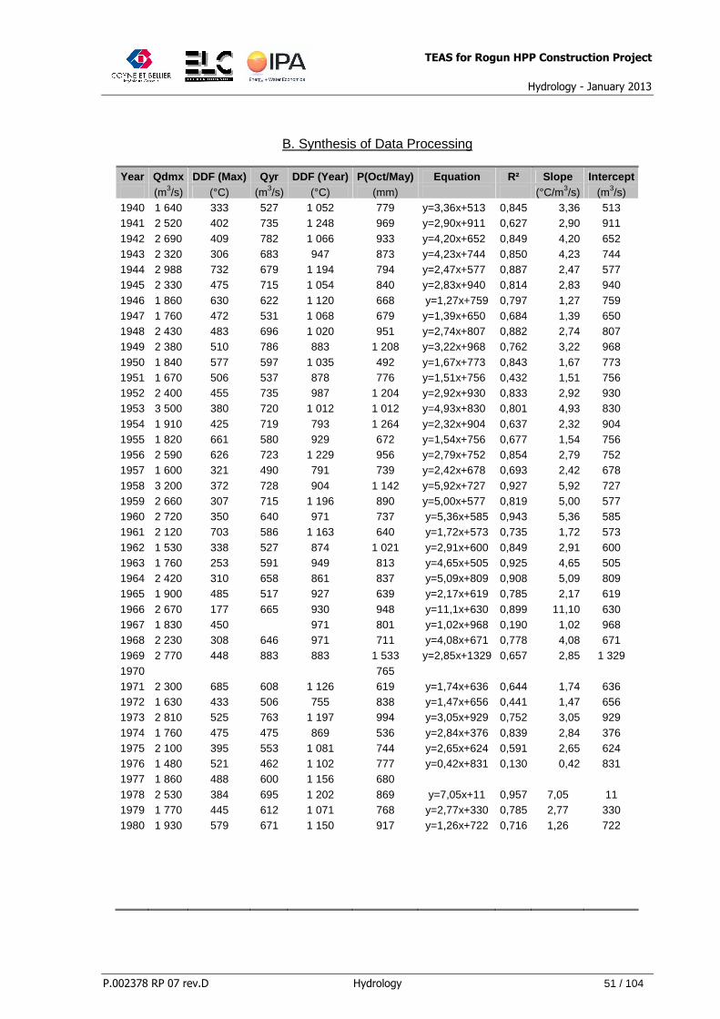
B. Synthesis of Data Processing
Year Qdmx DDF (Max) Qyr DDF (Year) P(Oct/May) Equation R² Slope Intercept (m3/s) (°C) (m3/s) (°C) (mm) (°C/m3/s) (m3/s)
1940 1 640 333 527 1 052 779 y=3,36x+513 0,845 3,36 513 1941 2 520 402 735 1 248 969 y=2,90x+911 0,627 2,90 911 1942 2 690 409 782 1 066 933 y=4,20x+652 0,849 4,20 652 1943 2 320 306 683 947 873 y=4,23x+744 0,850 4,23 744 1944 2 988 732 679 1 194 794 y=2,47x+577 0,887 2,47 577 1945 2 330 475 715 1 054 840 y=2,83x+940 0,814 2,83 940 1946 1 860 630 622 1 120 668 y=1,27x+759 0,797 1,27 759 1947 1 760 472 531 1 068 679 y=1,39x+650 0,684 1,39 650 1948 2 430 483 696 1 020 951 y=2,74x+807 0,882 2,74 807 1949 2 380 510 786 883 1 208 y=3,22x+968 0,762 3,22 968 1950 1 840 577 597 1 035 492 y=1,67x+773 0,843 1,67 773 1951 1 670 506 537 878 776 y=1,51x+756 0,432 1,51 756 1952 2 400 455 735 987 1 204 y=2,92x+930 0,833 2,92 930 1953 3 500 380 720 1 012 1 012 y=4,93x+830 0,801 4,93 830 1954 1 910 425 719 793 1 264 y=2,32x+904 0,637 2,32 904 1955 1 820 661 580 929 672 y=1,54x+756 0,677 1,54 756 1956 2 590 626 723 1 229 956 y=2,79x+752 0,854 2,79 752 1957 1 600 321 490 791 739 y=2,42x+678 0,693 2,42 678 1958 3 200 372 728 904 1 142 y=5,92x+727 0,927 5,92 727 1959 2 660 307 715 1 196 890 y=5,00x+577 0,819 5,00 577 1960 2 720 350 640 971 737 y=5,36x+585 0,943 5,36 585 1961 2 120 703 586 1 163 640 y=1,72x+573 0,735 1,72 573 1962 1 530 338 527 874 1 021 y=2,91x+600 0,849 2,91 600 1963 1 760 253 591 949 813 y=4,65x+505 0,925 4,65 505 1964 2 420 310 658 861 837 y=5,09x+809 0,908 5,09 809 1965 1 900 485 517 927 639 y=2,17x+619 0,785 2,17 619 1966 2 670 177 665 930 948 y=11,1x+630 0,899 11,10 630 1967 1 830 450 971 801 y=1,02x+968 0,190 1,02 968 1968 2 230 308 646 971 711 y=4,08x+671 0,778 4,08 671 1969 2 770 448 883 883 1 533 y=2,85x+1329 0,657 2,85 1 329 1970 765 1971 2 300 685 608 1 126 619 y=1,74x+636 0,644 1,74 636 1972 1 630 433 506 755 838 y=1,47x+656 0,441 1,47 656 1973 2 810 525 763 1 197 994 y=3,05x+929 0,752 3,05 929 1974 1 760 475 475 869 536 y=2,84x+376 0,839 2,84 376 1975 2 100 395 553 1 081 744 y=2,65x+624 0,591 2,65 624 1976 1 480 521 462 1 102 777 y=0,42x+831 0,130 0,42 831 1977 1 860 488 600 1 156 680 1978 2 530 384 695 1 202 869 y=7,05x+11 0,957 7,05 11 1979 1 770 445 612 1 071 768 y=2,77x+330 0,785 2,77 330 1980 1 930 579 671 1 150 917 y=1,26x+722 0,716 1,26 722

TEAS for Rogun HPP Construction Project
Hydrology - January 2013
P.002378 RP 07 rev.D Hydrology 52 / 104
Item Qdmx DDF (Max) Qyr DDF (Year) P(Oct/May) R² Slope Intercept N 40 40 39 40 41 39 39 39 M 2 206 453 640 1 015 854 0,745 3,18 708 S 492 127 98 132 206 0,185 1,97 215 Cv 0,223 0,281 0,154 0,130 0,241 0,248 0,620 0,303 Me 2 175 449 646 1 016 813 0,797 2,83 722 Max 3 500 732 883 1 248 1 533 0,957 11,10 1 329 Min 1 480 177 462 755 492 0,130 0,42 11
4.4.4. Maximisation Procedures to Obtain PMF
The next Table 10 details the relationships needed to estimate the daily peak by equations of
the following form:
• Qdmx = Slope x Degree-day factor at Peak + Intercept.
• Slope = f (Degree-day factor).
• Intercept = g (Seasonal Precipitation).
In such a model, the Consultant took into account both the precipitation (responsible for
available water amount) and the temperature (responsible for melt intensity) during the melt
season prior to the peak of discharge. The four graphs show that the relationships are
significant and that the proposed model is apt to reproduce observed daily peaks with an
underestimating bias of 11%.
On the two first graphs, the linear correlations obtained were drawn by taking into account
the set of 40 flood events. The R² values are about 0,42 / 0,44 which is significant although
indicating a scatter of data. Lower values would have been encountered in the 2006
approach when considering the whole data set instead of three subsets. For the slope versus
degree day factor, the trend is decreasing. Small degree day factor at yearly peak means
early flood and a larger slope (i.e. a larger amount of m3/s per °C/day). Large degree day at
yearly peak means late flood and a smaller slope (i.e. a smaller amount of m3/s per °C/day).
For the intercept versus seasonal precipitation, the trend is increasing. This means that
bigger precipitation will provide bigger floods. In addition to the correlation lines, some
envelopes were shown allowing for maximising observed events.

TEAS for Rogun HPP Construction Project
Hydrology - January 2013
P.002378 RP 07 rev.D Hydrology 53 / 104
The third graph displays the independence between seasonal precipitation and degree day
factor.
Finally, the fourth graph compares observed daily peak with computed peaks according to
the 40 relations detailed in the recapitulative table. There is a good adequacy but a bias of
11% is noticeable.
Table 10 - Slope and Intercept vs. Degree-day Facto r and Seasonal Precipitation
Slope vs. Degree Day Factor (DDF(Max))
y = -0,0102x + 7,78R 2 = 0,444
0
2
4
6
8
10
12
0 100 200 300 400 500 600 700 800
Degree Day Factor DDF (max) (°C)
Slo
pe (
m3/
s/°C
/day
)
Slope Envelope Linear - Slope
y=-0,0102x + 11,61

TEAS for Rogun HPP Construction Project
Hydrology - January 2013
P.002378 RP 07 rev.D Hydrology 54 / 104
Intercept vs. Seasonal Precipitation at Tavildara
y = 0,562x + 242R 2 = 0,417
0
200
400
600
800
1 000
1 200
1 400
1 600
0 200 400 600 800 1 000 1 200 1 400 1 600 1 800
Seasonal Precipitation at Tavildara - P(Oct / May) (mm)
Inte
rcep
t (m
3/s)
Intercept Envelope Intercept vs. Seasonal Precipitation
y=0,562x + 610
Degree Day Factor (SDD(Max)) vs. Seasonal Precipita tion at Tavildara
R 2 = 0,0595
0
100
200
300
400
500
600
700
800
0 200 400 600 800 1 000 1 200 1 400 1 600 1 800
Seasonal Precipitation at Tavildara - P (Oct / May) (mm)
Deg
ree
Day
Fac
tor
for
the
Max
imum
Dai
ly
Dis
char
ge (
°C)
SDD (Max) SDD(Max) vs. P(Oct / May)
SDD (Max) and P(Oct / May) are independent.

TEAS for Rogun HPP Construction Project
Hydrology - January 2013
P.002378 RP 07 rev.D Hydrology 55 / 104
Test of Model Adequacy
0
500
1 000
1 500
2 000
2 500
3 000
3 500
4 000
0 500 1 000 1 500 2 000 2 500 3 000 3 500
Computed Maximum Max(Computed) (m3/s)
Obs
erve
d M
axim
um D
isch
arge
Max
(Obs
erve
d)
(m3/
s)
Max (Observed) y=1,11x BI BS
R²=0,789
4.4.5. First Maximisation:
The Consultant proceeded to a first maximisation by considering the frequency distribution
of seasonal rainfall and degree day-factor at peak. The next Table details this first
maximisation.
It was found that a Root-Gauss distribution was suitable for the two independent variables as
shown by the two graphs. Thus it was possible to compute the slope and intersect
parameters for extreme degree-day factors and extreme seasonal precipitation. This
computation is summarised by part B in which the frequency domain varies from 0,90 to
0,9999. Such a scatter is consistent since it was shown that seasonal precipitation and
degree day factors are independent.
From 10 realisations of intercept and 10 realisations of the product (slope x degree day
factor), the Consultant deduced 100 flood peaks candidates for PMF. Part C details this first
maximisation.

TEAS for Rogun HPP Construction Project
Hydrology - January 2013
P.002378 RP 07 rev.D Hydrology 56 / 104
By this first approach, the PMF amounts to 6 710 m3/s that is 1,92 times the maximum
observed daily peak of 3 500 m3/s.
Table 11 - First Maximisation - Using Frequency Dis tributions
A. Frequency Distribution for Degree-Day Factor and for Seasonal Precipitation
Degree day Factor vs. Gauss Variate
0
100
200
300
400
500
600
700
800
-2,5 -2 -1,5 -1 -0,5 0 0,5 1 1,5 2 2,5
Gauss Variate u(Gauss)
Deg
ree
Day
Fac
tor
DD
F (
Max
) (°
C)
SDD (Max) Root-Gauss
Seasonal Precipitation at Tavildara vs. Gauss Varia te
0
200
400
600
800
1 000
1 200
1 400
1 600
1 800
-2,5 -2 -1,5 -1 -0,5 0 0,5 1 1,5 2 2,5
Gauss Variate u(Gauss)
Sea
sona
l Pre
cipi
tatio
n P
(Oct
/ M
ay)
(mm
)
P(Oct/May) Root-Gauss

TEAS for Rogun HPP Construction Project
Hydrology - January 2013
P.002378 RP 07 rev.D Hydrology 57 / 104
B. Intercept and Slope vs. Frequency
Fr u(Gauss) P(Oct/May) Intercept DDF(Max) Slope Product (mm) (m3/s) (°C) (m3/s) (m3/s)
0,9000 1,2816 1 115 1 237 623 5,26 3 274 0,9500 1,6449 1 199 1 284 679 4,69 3 181 0,9800 2,0537 1 298 1 339 745 4,01 2 989 0,9900 2,3263 1 365 1 377 790 3,55 2 804 0,9950 2,5758 1 429 1 413 833 3,55 2 957 0,9980 2,8782 1 508 1 457 887 3,55 3 147 0,9990 3,0902 1 564 1 489 926 3,55 3 284 0,9995 3,2905 1 619 1 520 963 3,55 3 416 0,9998 3,5401 1 688 1 558 1 010 3,55 3 584 0,9999 3,7190 1 738 1 587 1045 3,55 3707
C. First Maximisation
Intercept
Product 1 237 1 284 1 339 1 377 1 413 1 457 1 489 1 520 1 558 1 587 3 274 5 010 5 060 5 130 5 170 5 210 5 260 5 290 5 330 5 370 5 400 3 181 4 910 4 960 5 020 5 060 5 100 5 150 5 190 5 220 5 270 5 300 2 989 4 700 4 750 4 810 4 850 4 890 4 940 4 980 5 010 5 050 5 080 2 804 4 490 4 540 4 600 4 650 4 690 4 740 4 770 4 800 4 850 4 880 2 957 4 660 4 710 4 770 4 820 4 860 4 900 4 940 4 970 5 020 5 050 3 147 4 870 4 920 4 980 5 030 5 070 5 120 5 150 5 180 5 230 5 260 3 284 5 020 5 080 5 140 5 180 5 220 5 270 5 300 5 340 5 380 5 410 3 416 5 170 5 220 5 280 5 330 5 370 5 410 5 450 5 480 5 530 5 560 3 584 5 360 5 410 5 470 5 510 5 550 5 600 5 640 5 670 5 710 5 740 3 707 5 490 5 550 5 610 5 650 5 690 5 740 5 770 5 810 5 850 5 880
(m3/s) Item Result Result/ 3 500
n 100 M 5 178 1,48 S 323 Cv 0,062 Me 5 170 1,48 Max 5 880 1,68 Min 4 490 1,28 PMF (daily) 6 390 1,83 PMF (peak) 6 710 1,92
(m3/s)

TEAS for Rogun HPP Construction Project
Hydrology - January 2013
P.002378 RP 07 rev.D Hydrology 58 / 104
4.4.6. Second Maximisation:
For the second maximisation , the Consultant made use of the envelope curves defined for
slope and intercept parameters. The associated Table discloses that a daily PMF of
5 830 m3/s is obtained whereas the upper bound for PMF is 7 130 m3/s. Part A lists the 40
flood events considered. In this table the input data is recalled (DDF and P), the envelope
parameters (slope and intercept) together with observed and maximised daily peaks. Part B
gives the results of the second maximisation. On the basis of the mean maximised daily peak
(4 433 m3/s) and its standard deviation (374 m3/s), it was found that a daily PMF of
5 830 m3/s is acceptable. Making use of the ratio 5 830 / (Observed daily peak), a possible
upper bound of 6 790 m3/s for the daily peak was derived.
Table 11: Second Maximisation - Using 40 Flood Even ts
A. Table of Observed and Maximised Events
Input Data Envelope Parameters Daily Peaks Ratios
Year DDF(Max) P(Oct/May) Slope-max Intercept-max Observed Maximised Maxim./Obs 5830/Qdmx
(°C) (mm) (m3/s/°C) (m3/s) (m3/s) (m3/s)
1953 380 1 012 7,73 1 179 3 500 4 450 1,27 1,67
1958 372 1 142 7,82 1 252 3 200 4 480 1,40 1,82
1944 732 794 4,14 1 056 2 988 4 430 1,48 1,95
1973 525 994 6,26 1 169 2 810 4 820 1,72 2,07
1969 448 1 533 7,04 1 471 2 770 4 980 1,80 2,10
1960 350 737 8,04 1 024 2 720 4 150 1,53 2,14
1942 409 933 7,44 1 134 2 690 4 520 1,68 2,17
1966 177 948 9,80 1 143 2 670 3 070 1,15 2,18
1959 307 890 8,48 1 110 2 660 4 000 1,50 2,19
1956 626 956 5,22 1 147 2 590 4 780 1,85 2,25
1978 384 869 7,69 1 098 2 530 4 380 1,73 2,30
1941 402 969 7,51 1 154 2 520 4 510 1,79 2,31
1948 483 951 6,68 1 144 2 430 4 730 1,95 2,40
1964 310 837 8,45 1 081 2 420 3 990 1,65 2,41
1952 455 1 204 6,97 1 287 2 400 4 810 2,00 2,43
1949 510 1 208 6,41 1 289 2 380 4 920 2,07 2,45
1945 475 840 6,76 1 082 2 330 4 650 2,00 2,50
1943 306 873 8,49 1 100 2 320 3 990 1,72 2,51
1971 685 619 4,62 958 2 300 4 480 1,95 2,53
1968 308 711 8,47 1 009 2 230 3 910 1,75 2,61
1961 703 640 4,44 970 2 120 4 440 2,09 2,75
1975 395 744 7,58 1 028 2 100 4 360 2,08 2,78
1980 579 917 5,70 1 125 1 930 4 800 2,49 3,02
1954 425 1 264 7,28 1 320 1 910 4 760 2,49 3,05
1965 485 639 6,66 969 1 900 4 560 2,40 3,07
1946 630 668 5,18 985 1 860 4 620 2,48 3,13
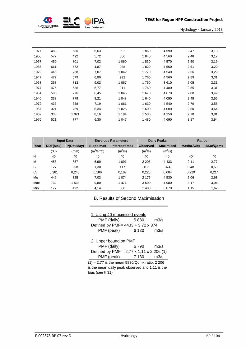
TEAS for Rogun HPP Construction Project
Hydrology - January 2013
P.002378 RP 07 rev.D Hydrology 59 / 104
1977 488 680 6,63 992 1 860 4 590 2,47 3,13
1950 577 492 5,72 886 1 840 4 560 2,48 3,17
1967 450 801 7,02 1 060 1 830 4 570 2,50 3,19
1955 661 672 4,87 988 1 820 4 560 2,51 3,20
1979 445 768 7,07 1 042 1 770 4 540 2,56 3,29
1947 472 679 6,80 992 1 760 4 560 2,59 3,31
1963 253 813 9,03 1 067 1 760 3 610 2,05 3,31
1974 475 536 6,77 911 1 760 4 480 2,55 3,31
1951 506 776 6,45 1 046 1 670 4 670 2,80 3,49
1940 333 779 8,21 1 048 1 640 4 090 2,49 3,55
1972 433 838 7,19 1 081 1 630 4 540 2,79 3,58
1957 321 739 8,34 1 025 1 600 4 000 2,50 3,64
1962 338 1 021 8,16 1 184 1 530 4 250 2,78 3,81
1976 521 777 6,30 1 047 1 480 4 690 3,17 3,94
Input Data Envelope Parameters Daily Peaks Ratios
Year DDF(Max) P(Oct/May) Slope-max Intercept-max Observed Maximised Maxim./Obs 5830/Qdmx
(°C) (mm) (m3/s/°C) (m3/s) (m3/s) (m3/s)
N 40 40 40 40 40 40 40 40
M 453 857 6,99 1 091 2 206 4 433 2,11 2,77
S 127 208 1,30 117 492 374 0,48 0,59
Cv 0,281 0,243 0,186 0,107 0,223 0,084 0,229 0,214
Me 449 825 7,03 1 074 2 175 4 530 2,06 2,68
Max 732 1 533 9,80 1 471 3 500 4 980 3,17 3,94
Min 177 492 4,14 886 1 480 3 070 1,15 1,67
B. Results of Second Maximisation
1. Using 40 maximised events PMF (daily) 5 830 m3/s
Defined by PMF= 4433 + 3,72 x 374 PMF (peak) 6 130 m3/s
2. Upper bound on PMF
PMF (daily) 6 790 m3/s Defined by PMF = 2,77 x 1,11 x 2 206 (1)
PMF (peak) 7 130 m3/s (1) – 2.77 is the mean 5830/Qdmx ratio, 2 206
is the mean daily peak observed and 1.11 is the bias (see § 31)

TEAS for Rogun HPP Construction Project
Hydrology - January 2013
P.002378 RP 07 rev.D Hydrology 60 / 104
C. Illustration of Second Maximisation
Maximisation of 40 Flood Events
3 000
3 500
4 000
4 500
5 000
5 500
6 000
6 500
7 000
1 000 1 200 1 400 1 600 1 800 2 000 2 200 2 400 2 600 2 800 3 000 3 200 3 400 3 600 3 800
Observed Maximum Daily Peak (m3/s)
Max
imis
ed D
aily
Pea
k (m
3/s)
Qdmx-Maximised PMF (daily) Upper Bound (PMF-daily)
4.4.7. Third Maximisation:
The third maximisation corresponds to a hypothetical case for which degree day and
seasonal precipitation are linked. For this, the Consultant adopted a rank correlation
approach.
In this approach, the Consultant defined a multiple correlation between daily peak discharge
as a dependent variable and degree day factor together with seasonal rainfall as
independent variables, but after having ranked separately the three samples (DDF, Qdmx
and P(Oct/May)) in ascending order.
The following equation was obtained:
Qdmx = 1,165 x P(Oct/May) + 1,903 x DDF + 345. (R²=0;956).

TEAS for Rogun HPP Construction Project
Hydrology - January 2013
P.002378 RP 07 rev.D Hydrology 61 / 104
This formula was applied for several values of DDF and P(Oct / May) providing estimates of
maximised daily discharges. Next Table details the third maximisation. It shows successively
the graphical description of the initial samples, the table of maximised daily peaks and the
final results.
The first graph displays the relationship (presented for P = 500, 1 000 and 1 500 mm)
together with the real set of data (DDF and Qdmx values).
The second graph shows the ranked values allowing for finding the model equation. Table B
gives 5 PMF candidates based on extreme events.
Table B gives also our estimate of PMF (daily PMF = 5 600 m3/s and instantaneous
PMF = 5 880 m3/s).
Table 12:Third Maximisation - Station Year Approach
A. Graphical Display of multiple correlation on Ranked values (2 graphs)
0
500
1 000
1 500
2 000
2 500
3 000
3 500
4 000
0 100 200 300 400 500 600 700 800
Max
imum
Dai
ly D
isch
arge
(m3/
s)
Degree Day Factor SDD (Max) (°C)
Maximum Daily Discharge vs. Degree-Day Factor and S easonal Precipitation
Max (Qdmx) P=500 P=1 000 P= 1500
Qdmx = 1,903 DDF + 1,165 P (Oct/May) + 345

TEAS for Rogun HPP Construction Project
Hydrology - January 2013
P.002378 RP 07 rev.D Hydrology 62 / 104
TB. Table of Maximised Daily Floods (m3/s)
T (years) Pseas (mm) SDD (°C) Qdmax (m3/s) 10 000 1 738 1 045 4 360
20 000 1 787 1 079 4 480
50 000 1 850 1 122 4 640 100 000 1 896 1 154 4 760
200 000 1 942 1 186 4 870
500 000 2 0001 226 5 010
1 000 000 2 044 1 257 5 120
N 5 M 4 880 S 191
Cv 0,039 Me 4 870
Max 5 120
Min 4 640
PMF (daily) 5 600
PMF (peak) 5 880
Data for Ranked Correlation
R2 = 0,946
R2 = 0,943
0
500
1 000
1 500
2 000
2 500
3 000
3 500
4 000
0 100 200 300 400 500 600 700 800
Ranked Degree-Day Factor (°C)
Ran
ked
Dis
char
ge a
nd R
anke
d P
reci
pita
tion
P* Max(Obs) P* Q Max

TEAS for Rogun HPP Construction Project
Hydrology - January 2013
P.002378 RP 07 rev.D Hydrology 63 / 104
4.4.8. PMF Choice and PMF Hydrograph
Computation of flood hydrographs is based on three major observed floods at Tutkaul. These
floods are:
• July 1953 the largest flood recorded on the Vakhsh, with daily discharge of 3500 m3/s
and a peak discharge of 3730 m3/s. Note that first estimation of peak discharge was
4290 m3/s but was recalculated in 1978 for Rogun Project Report by Hydroproject
(1978),
• July 1958, with a daily discharge of 3250 m3/s,
• July 1969, with a daily discharge of 2800 m3/s, but this flood is the major event in
terms of volume recorded on the Vakhsh.
The choice of an a-dimensional hydrograph shape was made in order to combine the aspect
of flood peaking issued from July 1953 and July 1958, and flood volume from July 1969. The
peak coefficient was derived from observed discharge made in July 1953, and equals 1.05.
The following Table summarises the obtained results and the choice of PMF together with a
plot of the PMF hydrograph. In part A the various PMF estimates were ranked in ascending
order. The rank correlation (third maximisation) is the smallest estimate ( 5 600 m3/s)
followed by the maximisation of 40 floods (second maximisation, 5 830 m3/s). The frequency
approach (first maximisation) arrives at the third place with a daily peak of 6 390 m3/s. As
shown in the observation column, these three estimates are within the domain of the 10 000
year flood. Thus, they are discarded for the choice of PMF.
The upper bound of the maximisation of 40 floods together with the PMF estimate of 2006
are retained. They provide a mean value of 6 950 m3/s associated to a standard deviation of
220 m3/s. These results lead to recommend a daily PMF of 7 770 m3/s associated to an
instantaneous peak of 8 160 m3/s.

TEAS for Rogun HPP Construction Project
Hydrology - January 2013
P.002378 RP 07 rev.D Hydrology 64 / 104
Table 13: PMF Choice and PMF Hydrograph
A. PMF Choice
Approach PMF (daily) PMF (peak) Peak / 5 970 Observations
(m3/s) (m3/s) Ranked Correlation (3rd maxim.) 5 600 5 880 0,98 Domain Maximisation of 40 floods (2nd maxim.) 5 830 6 130 1,03 of the Frequency approach (1st maxim) 6 390 6 710 1,12 10 000 yr flood 2nd maxim.- Upper Bound 6 790 7 130 1,19 Retained 2006 – approach (Lahmeyer) 7 100 7 460 1,25 Retained M 6 950 Of retained values S 220 Of retained values Proposed PMF: M+3,72S 7 770 8 160 1,42
B. PMF Hydrograph
Hydrographs for 10 000-yr Flood and Probable Maximu m Flood
0
1 000
2 000
3 000
4 000
5 000
6 000
7 000
8 000
9 000
0 20 40 60 80 100 120 140 160 180 200 220 240 260 280 300 320 340 360 380
Day N° (1 is January 1st)
Dai
ly D
isch
arge
(m
3/s)
10 000 yr PMF

TEAS for Rogun HPP Construction Project
Hydrology - January 2013
P.002378 RP 07 rev.D Hydrology 65 / 104
5. CLIMATE CHANGE
The Consultant tried to develop its own approach based on trend analysis of historical data
as well as available literature on Climate Change in Central Asia and Tajikistan. Even if
downscaling of climate models to local conditions is still subject to lot of uncertainties, this
approach of confronting deducted trends to global models results was found useful in order
to define potential scenarios.
The study was therefore conducted in the following steps:
• Firstly an analysis of the observed trends concerning the period 1930 / 2010 for
precipitation, discharge, and temperatures. The correlations found are not fully
convincing, but some trend for increased precipitation and discharges could be
assumed. Concerning temperatures at Anzob Pass and Tavildara, there is no
significant trend. For Gorbunov (Fedchenko Glacier), an increase of 0,5°C per 100
years is noticeable but linked to a weak R² (0,190). It is however in the same order of
magnitude as existing models.
• Thereafter, a review of the literature quoted in the reference list was made to obtain a
general understanding of the current status of Climate Change predictions in Central
Asia and Tajikistan. It became obvious from the extensive records that glacier melt
was an important issue, and a recorded fact based on a close monitoring of Glaciers
in Central Asia. Data enclosed in Aral Sea depletion studies indicate that as per
projections, in 2080 / 2100, the glaciers feeding Aral Sea could disappear. Studies
carried out by Tajik institutes clearly show that the glaciers are receding.
• It was therefore found of interest to carry out a specific analysis about glacier
vanishing and try to evaluate its impact on Vakhsh river regime. After this specific
study about the vanishing of glacier, the Consultant tried to make an assessment of
the evolution of Vakhsh discharges under the assumption of a discharge increasing
trend (at same level as the historical trend) associated to an ice feeding reduction due
to temperature increase as suggested by the Climate Models.

TEAS for Rogun HPP Construction Project
Hydrology - January 2013
P.002378 RP 07 rev.D Hydrology 66 / 104
5.1 Data for Climate Change Analysis
Data for climate change study is either included in the main text or in the supporting
documents. These data have been taken from previous reports, from data provided by the
Client or data found in the existing literature (see references).
The main inputs for this climate change study are:
• For Trend Analysis: Yearly and seasonal discharges; yearly temperatures; yearly
precipitations (1932/2010)
• For Climate Forecasts: Increase / Decrease of temperature as given by several
climate models. Percentage change of precipitation as given by several climate
models. Forecast about glacier melts as given by several researchers about
Central Asia and Aral Sea Basin (see reference list).
5.2 Trend Analysis of Precipitation, Temperature an d Discharge
5.2.1 Trend Analysis of Precipitation
The following Table 4 presents the results of our trend analysis for precipitation. It consists of
three tables and five graphs. Part A details the available data concerning five rain gauges:
Racht, Altynmazar, Komsomolabad and Tavildara. Part B illustrates the graphs of
precipitation time series. The trends were computed using the 5-year moving averages. The
R² values are often rather weak, but trends can be assessed from the observed data. Part C
presents the results and gives a forecast of average precipitation and yearly discharge until
2100. If precipitation trends are not modified, the rainfall and runoff could increase by about
15% by 2100. Such increase is in line with a temperature increase resulting in a more humid
atmospheric column. As it will be detailed in the general review of existing climate change
models, precipitation trends are difficult to determine and still subject to a large uncertainty.
Consequently, a no change option is still the most prudent scenario to be considered for
precipitation trend forecast.

TEAS for Rogun HPP Construction Project
Hydrology - January 2013
P.002378 RP 07 rev.D Hydrology 67 / 104
Table 14: Trend Analysis of Precipitation Data
A. Yearly Precipitation Data
Year Racht Altynmazar Komsomolabad Anzob Tavildara 1933 700 157 620 1934 807 91 1 035 1935 872 155 1 047 1936 501 128 642 1937 741 185 944 1938 542 106 661 1939 753 119 946 1940 599 120 268 790 1941 736 157 248 910 1942 791 155 349 1 045 1943 717 145 285 1 012 1944 574 117 230 724 1945 195 263 921 1946 154 259 630 1947 473 94 271 654 1948 851 180 1 008 313 1 150 1949 932 247 1 136 318 1 179 1950 512 84 675 270 568 1951 817 233 941 595 1 001 1952 929 139 1 176 528 1 065 1953 1 260 331 1 376 572 1 480 1954 817 213 919 457 978 1955 654 115 865 266 855 1956 703 133 864 216 806 1957 816 177 1 028 511 1 050 1958 1 008 223 1 129 498 1 186 1959 635 109 709 514 839 1960 904 172 869 510 842 1961 588 123 758 384 714 1962 686 131 887 511 1 056 1963 765 144 887 739 781 1964 837 194 758 482 918 1965 735 168 872 382 848 1966 763 212 964 470 1 088 1967 611 119 811 354 809 1968 909 167 1 038 451 943 1969 1 336 240 1 539 590 1 525 1970 708 150 838 491 771 1971 439 88 590 230 580 1972 833 171 973 529 959 1973 729 177 868 443 893 1974 784 167 814 500 825 1975 685 111 751 505 791 1976 690 179 901 518 842

TEAS for Rogun HPP Construction Project
Hydrology - January 2013
P.002378 RP 07 rev.D Hydrology 68 / 104
Year Racht Altynmazar Komsomolabad Anzob Tavildara 1977 660 174 797 520 914 1978 736 143 891 534 817 1979 584 153 767 456 718 1980 797 159 937 468 1 048 1981 897 187 1 116 527 1 120 1982 718 168 870 542 843 1983 589 122 680 470 765 1984 687 142 999 464 1 102 1985 612 165 805 438 943 1986 625 157 786 411 855 1987 946 261 1 081 548 1 357 1988 781 224 870 466 1 031 1989 720 145 758 478 948 1990 770 138 970 509 922 1991 1 018 257 1 266 728 1 336 1992 766 150 571 1 107 1993 911 269 847 1 358 1994 763 87 591 1 012 1995 519 248 306 656 1996 651 382 807 1997 607 460 834 1998 890 537 1 482 1999 769 462 2000 686 249 2001 593 129 2002 828 237 2003 707 395 2004 905 722 2005 696 474 2006 667 542 2007 843 492 2008 583 272 2009 929 541 2010 1 002 349 N 76 63 44 71 66 M 753 164 921 443 938 S 159 50 185 138 216 Cv 0,211 0,307 0,201 0,312 0,231 Me 736 157 879 468 919 Max 1 336 331 1 539 847 1 525 Min 439 84 590 129 568
(mm/year)
TEAS for Rogun HPP Construction Project
Hydrology - January 2013
P.002378 RP 07 rev.D Hydrology 69 / 104
B. Graphs about Precipitation Trend
Racht - Yearly Precipitation
y = 0,249x + 256R 2 = 0,007
400
500
600
700
800
900
1 000
1 100
1 200
1 300
1 400
1920 1930 1940 1950 1960 1970 1980 1990 2000 2010 2020
Years
Yea
rly P
reci
pita
tion
Pyr
(m
m)
Racht MAV-5yr M=753 Trend based on 5-yr moving average
Altynmazar - Yearly Precipitation
y = 0,531x - 879R 2 = 0,205
50
100
150
200
250
300
350
1920 1930 1940 1950 1960 1970 1980 1990 2000
Years
Yea
rly P
reci
pita
tion
Pyr
(m
m)
Altynmazar MAV-5yr M=164 Trend based on 5-yr moving average

TEAS for Rogun HPP Construction Project
Hydrology - January 2013
P.002378 RP 07 rev.D Hydrology 70 / 104
Komsomolabad - Yearly Rainfall
y = -2,90x + 6627R 2 = 0,195
500
700
900
1 100
1 300
1 500
1 700
1945 1950 1955 1960 1965 1970 1975 1980 1985 1990 1995
Years
Yea
rly P
reci
pita
tion
Pyr
(m
m)
Komsomolabad MAV-5yr M=921 Trend based on 5-yr moving average
Anzob - Yearly Precipitation
y = 1,81x - 3 131R 2 = 0,168
100
200
300
400
500
600
700
800
900
1930 1940 1950 1960 1970 1980 1990 2000 2010 2020
Years
Yea
rly P
reci
pita
tion
Pyr
(m
m)
Anzob MAV-5yr M=443 Trend based on 5-yr moving average

TEAS for Rogun HPP Construction Project
Hydrology - January 2013
P.002378 RP 07 rev.D Hydrology 71 / 104
Tavildara - Yearly Precipitation
y = 2,20x - 3395R 2 = 0,197
400
600
800
1 000
1 200
1 400
1 600
1920 1930 1940 1950 1960 1970 1980 1990 2000 2010
Years
Yea
rly P
reci
pita
tion
Pyr
(m
m)
Tavildara MAV-5yr M=443 Trend based on 5-yr moving average
C. Results concerning Precipitation Trend
Observed Trend
Station Period n M(Pyr) Trend (mm/yr) Trend (%) R² Trend(%) x R²
Altynmazar 1933-1995 63 164 0,53 0,32 0,205 0,066 Anzob 1940-2010 71 443 1,81 0,41 0,168 0,069 Racht 1933-2010 76 753 0,25 0,03 0,007 0,000 Komsomolabad 1948-1991 44 921 -2,90 -0,31 0,195 -0,061 Tavildara 1933-1998 66 938 2,20 0,23 0,197 0,046 Average 0,14 % Regional trend 0,16 %
TEAS for Rogun HPP Construction Project
Hydrology - January 2013
P.002378 RP 07 rev.D Hydrology 72 / 104
Precipitation Forecast Year Pyr % Change % Tavildara Seasonal Qyr % Change
(mm) (mm) (m3/s) 2010 1 090 100,0 0,0 866 638 100,0 0,0 2015 1 099 100,8 0,8 873 643 100,8 0,8 2020 1 108 101,6 1,6 880 648 101,6 1,6 2025 1 116 102,4 2,4 887 653 102,4 2,4 2030 1 125 103,2 3,2 894 658 103,2 3,2 2035 1 134 104,1 4,1 901 663 104,0 4,0 2040 1 144 104,9 4,9 908 669 104,8 4,8 2050 1 162 106,6 6,6 923 679 106,5 6,5 2055 1 171 107,5 7,5 930 684 107,3 7,3 2060 1 181 108,3 8,3 938 690 108,1 8,1 2065 1 190 109,2 9,2 945 695 109,0 9,0 2070 1 200 110,1 10,1 953 701 109,8 9,8 2075 1 209 111,0 11,0 961 706 110,7 10,7 2080 1 219 111,8 11,8 968 712 111,6 11,6 2085 1 229 112,7 12,7 976 717 112,4 12,4 2090 1 239 113,6 13,6 984 723 113,3 13,3 2095 1 249 114,6 14,6 992 729 114,2 14,2 2100 1 259 115,5 15,5 1 000 734 115,1 15,1
5.2.2 Trend Analysis of Temperature
The analysis of temperature trend was based on three stations: Fedchenko (Gorbunov),
Anzob Pass and Tavildara. These stations are in a mountainous context. Part A details the
available data concerning these three stations. Part B illustrates the graphs of precipitation
time series. Trends were computed using the 5-year moving averages. The R² values are
often rather weak, but trends can be assessed for Tavildara and Fedchenko (Gorbunov). For
Tavildara, the observed trend is about 0,8°C per century and for Fedchenko (Gorbunov) it is
0,5°C per century . These trends are much smaller than those given by the climate change
models, but in a rather similar range of magnitude.

TEAS for Rogun HPP Construction Project
Hydrology - January 2013
P.002378 RP 07 rev.D Hydrology 73 / 104
Table 15: Trend Analysis of Temperature Data
A. Yearly Temperature Data
Year Gorbunov Anzob Pass Tavildara 1934 -8,2 1935 -7,4 1936 -7,3 1937 -7,3 1938 -7,1 1939 -6,9 1940 -5,7 -0,60 1941 -6,4 -0,46 1942 -7,1 -1,47 1943 -7,0 -2,33 1944 -7,4 -1,60 1945 -7,4 -2,26 1946 -6,5 -1,18 1947 -7,3 -1,11 1948 -7,6 -2,11 1949 -7,6 -2,90 1950 -6,8 -2,69 1951 -6,7 -2,31 1952 -7,8 -1,70 1953 -7,1 -1,99 1954 -6,0 -2,63 1955 -8,1 -1,62 1956 -7,0 -0,93 1957 -6,7 -3,04 1958 -7,2 -1,72 1959 -7,1 -1,36 1960 -7,4 -1,99 1961 -7,7 -1,71 9,1 1962 -7,4 -2,27 8,6 1963 -7,3 -1,02 9,6 1964 -7,4 -2,83 7,6 1965 -7,3 -1,87 8,8 1966 -7,1 -1,57 9,5 1967 -6,8 -2,30 8,6 1968 -6,2 -2,23 8,6 1969 -7,6 -2,61 8,0 1970 -6,3 -1,35 9,7 1971 -7,6 -0,76 10,0 1972 -7,4 -2,99 7,7 1973 -7,0 -1,10 9,6 1974 -6,2 -2,69 8,2 1975 -7,8 -2,10 8,2 1976 -6,3 -2,36 8,9 1977 -7,6 -0,97 10,5

TEAS for Rogun HPP Construction Project
Hydrology - January 2013
P.002378 RP 07 rev.D Hydrology 74 / 104
Year Gorbunov Anzob Pass Tavildara 1978 -7,4 -1,43 9,2 1979 -7,0 -1,00 9,8 1980 -6,2 -1,01 9,9 1981 -6,3 9,0 1982 -6,6 8,1 1983 -6,1 9,0 1984 -6,9 8,5 1985 -7,3 9,1 1986 -6,9 8,7 1987 -6,9 8,9 1988 -6,2 9,6 1989 -7,9 7,9 1990 -6,1 9,7 1991 -7,1 1992 -7,0 1993 -7,2 1994 -6,8 1995 N 61 41 30 M -7,0 -1,8 9,0 S 0,6 0,7 0,7 Cv -0,080 -0,390 0,083 Me -7,1 -1,7 9,0 Max -5,7 -0,5 10,5 Min -8,2 -3,0 7,6
(°C)

TEAS for Rogun HPP Construction Project
Hydrology - January 2013
P.002378 RP 07 rev.D Hydrology 75 / 104
B. Graphs about Temperature Trend
Gorbunov (Fedchenko Glacier) - Yearly Temperature
y = 0,005x - 16,6R 2 = 0,105
-8,5
-8,0
-7,5
-7,0
-6,5
-6,0
-5,5
-5,0
1930 1940 1950 1960 1970 1980 1990 2000
Years
Yea
rly T
eper
atur
e T
yr (
°C°
Gorbunov Mav-5yr Mean (61/90)=-6,9°C Trend Based on 5-year moving average
Anzob Pass - Yearly Temperature
R 2 = 0,0003
-3,50
-3,00
-2,50
-2,00
-1,50
-1,00
-0,50
0,00
1935 1940 1945 1950 1955 1960 1965 1970 1975 1980 1985
Years
Yea
rly T
empe
ratu
re T
yr (
°C)
Tyr (°C) MAV-5yr M(40yrs)=-1,81 Trend based on 5-yr moving average
TEAS for Rogun HPP Construction Project
Hydrology - January 2013
P.002378 RP 07 rev.D Hydrology 76 / 104
Tavildara - Yearly Temperature
y = 0,009x - 8,71R 2 = 0,058
6,0
6,5
7,0
7,5
8,0
8,5
9,0
9,5
10,0
10,5
11,0
1955 1960 1965 1970 1975 1980 1985 1990 1995
Years
Yea
rly T
empe
ratu
re T
yr (
°C)
Tyr - Tavildara Mav-5yr M=9,0°C Trend based on 5-yr average
5.2.3 Trend Analysis of Discharges
The following Table 16 details our trend analysis for discharges. The coefficients of
correlation R² are rather weak. The best R² is obtained for the cold season discharge (base
flow). An increase of discharge of about 0,26 / 0,30 m3/s/year could be assumed. The Table
presents forecast until 2100 according to these trends.

TEAS for Rogun HPP Construction Project
Hydrology - January 2013
P.002378 RP 07 rev.D Hydrology 77 / 104
Table 16: Trend Analysis of Discharges
A. Data about Observed Discharge
Year Annual IV-IX X-III 1932 - 1933 621 1 052 187 1933 - 1934 609 1 008 208 1934 - 1935 696 1 163 227 1935 - 1936 562 919 204 1936 - 1937 647 1 101 190 1937 - 1938 640 1 057 222 1938 - 1939 561 919 200 1939 - 1940 588 973 200 1940 - 1941 527 845 208 1941 - 1942 721 1 171 268 1942 - 1943 737 1 188 282 1943 - 1944 615 977 252 1944 - 1945 621 1 018 223 1945 - 1946 680 1 117 240 1946 - 1947 612 986 235 1947 - 1948 516 850 182 1948 - 1949 703 1 153 251 1949 - 1950 785 1 268 299 1950 - 1951 597 979 214 1951 - 1952 559 880 239 1952 - 1953 730 1 207 250 1953 - 1954 689 1 101 274 1954 - 1955 733 1 200 264 1955 - 1956 575 923 226 1956 - 1957 704 1 184 222 1957 - 1958 493 765 220 1958 - 1959 718 1 197 237 1959 - 1960 705 1 158 252 1960 - 1961 632 1 039 223 1961 - 1962 580 945 213 1962 - 1963 522 839 204 1963 - 1964 582 956 209 1964 - 1965 652 1 083 220 1965 - 1966 514 816 211 1966 - 1967 652 1 101 202 1967 - 1968 569 917 220 1968 - 1969 654 1 052 254 1969 - 1970 867 1 438 293 1970 - 1971 667 1 092 239 1971 - 1972 591 973 209 1972 - 1973 513 814 210 1973 - 1974 765 1 290 237 1974 - 1975 495 798 191 1975 - 1976 577 939 215

TEAS for Rogun HPP Construction Project
Hydrology - January 2013
P.002378 RP 07 rev.D Hydrology 78 / 104
1976 - 1977 578 933 221 Year Annual IV-IX X-III 1977 - 1978 624 1 017 228 1978 - 1979 705 1 160 248 1979 - 1980 634 1 032 236 1980 - 1981 650 1 088 209 1981 - 1982 630 1 017 241 1982 - 1983 583 930 233 1983 - 1984 631 1 044 219 1984 - 1985 667 1 104 227 1985 - 1986 613 997 226 1986 - 1987 529 825 232 1987 - 1988 701 1 136 266 1988 - 1989 736 1 255 215 1989 - 1990 450 678 220 1990 - 1991 652 1 037 265 1991 - 1992 611 988 234 1992 - 1993 718 1 214 219 1993 - 1994 699 1 141 254 1994 - 1995 758 1 285 228 1995 - 1996 596 953 239 1996 - 1997 626 962 288 1997 - 1998 599 900 295 1998 - 1999 819 1 309 326 1999 - 2000 619 1 007 230 2000 - 2001 570 932 207 2001 - 2002 569 913 223 2002 - 2003 710 1 183 235 2003 - 2004 651 1 079 223 2004 - 2005 656 1 050 261 2005 - 2006 732 1 209 252 2006 - 2007 638 1 044 230 2007 - 2008 747 1 262 233 n 76 76 76 M 638 1 041 233 S 80 145 28 Cv 0,126 0,139 0,118 Me 632 1 038 228 Max 867 1 438 326 Min 450 678 182

TEAS for Rogun HPP Construction Project
Hydrology - January 2013
P.002378 RP 07 rev.D Hydrology 79 / 104
B. Discharge Time Series
Vakhsh River at Rogun Damsite - Yearly Discharges - 1932/33 to 2007/08
y = 0,275x + 95R 2 = 0,040
400
450
500
550
600
650
700
750
800
850
900
1930 1935 1940 1945 1950 1955 1960 1965 1970 1975 1980 1985 1990 1995 2000 2005 2010
Water-Years
Yea
rly D
isch
arge
Qyr
(m
3/s)
0
5 000
10 000
15 000
20 000
25 000
30 000
35 000
40 000
45 000
50 000
Cum
ulat
ive
Yea
rly D
isch
arge
(m
3/s)
Qyear M = 638 MAV-5yr S-Qyr Trend based on 5yr moving average
Vakhsh River at Rogun Damsite - Melt Season Dischar ges - 1932/33 to 2007/08
y = 0,294x + 459R2 = 0,017
600
700
800
900
1 000
1 100
1 200
1 300
1 400
1 500
1930 1935 1940 1945 1950 1955 1960 1965 1970 1975 1980 1985 1990 1995 2000 2005 2010
Water-Years
Mel
t Sea
son
Dis
char
ge Q
IV-I
X (
m3/
s)
0
10 000
20 000
30 000
40 000
50 000
60 000
70 000
80 000
90 000
Cum
ulat
ive
Mel
t Sea
son
Dis
char
ge
(m3/
s)
QIV-IX M = 1 041 MAV-5yr S-QIV-IX Trend based on 5-yr moving average

TEAS for Rogun HPP Construction Project
Hydrology - January 2013
P.002378 RP 07 rev.D Hydrology 80 / 104
Vakhsh River at Rogun Damsite - Cold Season Discha rge - 1932/33 to 2007/08
y = 0,260x - 278R2 = 0,120
150
170
190
210
230
250
270
290
310
330
350
1930 1935 1940 1945 1950 1955 1960 1965 1970 1975 1980 1985 1990 1995 2000 2005 2010
Water-Years
Col
d S
easo
n D
isch
arge
QX
-III
(m3/
s)
0
2 000
4 000
6 000
8 000
10 000
12 000
14 000
16 000
18 000
20 000
Cum
ulat
ed C
old
Sea
son
Dis
char
ge
(m3/
s)
QX-III M = 233 MAV-5yr S-QX-III Trend based on 5-yr moving average
C. Results concerning Discharge Trend
Observed Trend
Period Mean (m3/s) Trend (m3/s/yr) Trend (%)
Year 638 0,275 0,043 Melt Season 1 041 0,294 0,028 Cold Season 233 0,260 0,112
Discharge Forecast
Year Mean Melt Season Cold Season Mean Melt Season Cold Season
(m3/s) (m3/s) (m3/s) (%) (%) (%) 2010 638 1 041 233 100,0 100,0 100,0 2015 639 1 042 234 100,2 100,1 100,6 2020 641 1 044 236 100,4 100,3 101,1 2025 642 1 045 237 100,6 100,4 101,7 2030 644 1 047 238 100,9 100,6 102,2 2035 645 1 048 240 101,1 100,7 102,8 2040 646 1 050 241 101,3 100,8 103,3 2045 648 1 051 242 101,5 101,0 103,9 2050 649 1 053 243 101,7 101,1 104,5 2055 650 1 054 245 101,9 101,3 105,0 2060 652 1 056 246 102,2 101,4 105,6 2065 653 1 057 247 102,4 101,6 106,1 2070 654 1 059 249 102,6 101,7 106,7 2075 656 1 060 250 102,8 101,8 107,3

TEAS for Rogun HPP Construction Project
Hydrology - January 2013
P.002378 RP 07 rev.D Hydrology 81 / 104
Year Mean Melt Season Cold Season Mean Melt Season Cold Season 2080 657 1 062 251 103,0 102,0 107,8 2085 659 1 063 252 103,2 102,1 108,4 2090 660 1 065 254 103,4 102,3 108,9 2095 661 1 066 255 103,7 102,4 109,5 2100 663 1 067 256 103,9 102,5 110,0
5.2.4 Existing models in Central Asia – Temperature and Precipitation Projections
This section presents the temperature and precipitation forecasts which are quoted in the
report of René Roy about Tajikistan and Kyrgyz Republic. Next Table details the values of
interest for Rogun project.
From René Roy report, the distribution of climate change given by several models for the
years 2020, 2050 and 2080 was extracted and extrapolated until 2100:
• For temperature the models are rather consistent since they all imply an increase of
temperature.
• For precipitation, as quoted by Roy and several other authors, the dispersion of the
results is of the same order of magnitude as the percentage change. Thus some
models forecast decrease of precipitation whereas some forecast increase of
precipitation, leading to opposite conclusions.
In part A, the anticipated temperature increase given by the climate models is presented. The
historical trend that could be assumed from trend analysis has also been added to the graph.
It is to be noted that the historic trend corresponds to an increase which is about one third of
the minimum increase given by climate models.
Part B concerns the change in precipitation. The wide scatter given by the climate models is
evident. The no change option corresponds more or less to the median results. The historical
trend, based on five rain gauges would lead to an increase of about 16% in 2100. The
historical trend is within the range provided by the climate models, but a no change option
would be a safe approach given the uncertainties carried by the models.

TEAS for Rogun HPP Construction Project
Hydrology - January 2013
P.002378 RP 07 rev.D Hydrology 82 / 104
Table 17: Climate Change in Central Asia - Temperat ure and Precipitation
A. Temperature Change (°C)
Year Min 25% 50% 75% Max Historical Trend 2020 0,6 1,1 1,4 1,6 2,3 0,2 2050 1,2 2,2 2,5 3,1 4,0 0,4 2080 1,7 2,9 3,6 4,5 5,9 0,6 2100 2,0 3,4 4,3 5,4 7,2 0,8
Central Asia - Temperature Changes with respect to 1980-1999 Conditions
0
1
2
3
4
5
6
7
8
2010 2020 2030 2040 2050 2060 2070 2080 2090 2100 2110
Years
Cha
nge
in M
ean
Tem
pera
ture
dT
yr (
°C)
Min 25% 50% 75% Max Historical Trend
B. Precipitaton Change (%)
Year Min 25% 50% 75% Max Historical Trend 1990 0,0 0,0 0,0 0,0 0,0 0,0 2020 -7,0 0,0 2,0 4,5 12,5 1,6 2050 -9,5 -1,0 1,5 5,0 15,0 6,6 2080 -12,5 -1,5 1,5 5,0 15,5 11,8 2100 -14,5 -1,8 1,5 5,0 15,8 15,5
TEAS for Rogun HPP Construction Project
Hydrology - January 2013
P.002378 RP 07 rev.D Hydrology 83 / 104
Central Asia - Precipitation Change from 1990 to 21 00
-17,5
-15
-12,5
-10
-7,5
-5
-2,5
0
2,5
5
7,5
10
12,5
15
17,5
1980 1990 2000 2010 2020 2030 2040 2050 2060 2070 2080 2090 2100 2110
Years
Pre
cipi
tatio
n C
hang
e dP
yr (
%)
Min 25% 50% 75% Max Historical Trend
5.3 Snow Accumulation and Glacier Melt
5.3.1. Analysis of Regional Information
Homidov (2006) and Makmadaliev, Novikov and al. (2002, 2003 and 2008) show that the
glacier are receding in Tajikistan. Analysis of present climate discloses that temperature can
either increase or decrease or remain stable according to the location. Roy (2009) and
Siegfried (2010) have reviewed data and results of climate change model for Central Asia.
Tajik experts forecast a disappearance of small glaciers and a decrease of about 50% of
glaciers in low elevations. At higher elevations and according to them the reduction could be
between 20 and 50% or smaller than 20%.
Next Table illustrates findings quoted by Tajik experts, Roy and Siegfried together with
extrapolations until 2100. Part A presents a broad picture of conditions in Tajikistan and
Kyrgyz Republic as presented by Roy. Roy evokes disappearance of glaciers. That might be
right for low and medium elevations. But, high altitude glaciers will still exist. Similarly, the
30% decrease of Amu Darya flows might be debatable. Such a value might be inapplicable

TEAS for Rogun HPP Construction Project
Hydrology - January 2013
P.002378 RP 07 rev.D Hydrology 84 / 104
to Vakhsh case. Roy quotes also a runoff decrease of 100 mm for Tajikistan. Transposed to
Vakhsh case, this would mean a reduction of 96 m3/s compared to the present average of
638 m3/s (a 15% reduction).
Part B details the decrease of Ice Reserve within Aral Sea Basin which, under the
assumption of linear correlation, might lead to a total disappearance before 2100. The
Consultant believes that such a strong linear assumption is not realistic. With an exponential
extrapolation, in 2100, Ice reserve could be 22% of 1957 value.
Part C concerns the Tien Shan glaciers for which Siegfried and others studied Ice reserves
for two climate scenarios. The lower one leads to an ice reserve of 87% of 1990 ice reserve,
whereas the higher one leads to an ice reserve of 44% of 1990 ice reserve.
As a conclusion part D compares Aral Sea and Tien Shan ice reserves. From this
comparison the Consultant has derived an average trend that could represent a realistic
assumption for Tajik glaciers. According to this average trend, in 2100, 36% of ice reserves
will remain in 2100.

TEAS for Rogun HPP Construction Project
Hydrology - January 2013
P.002378 RP 07 rev.D Hydrology 85 / 104
Table 18: Regional Information About Climate Change and Melt
A. Climate Evolution for Tajikistan and Kyrgyz Republic
Time Step Recent Past (1950 -2000) 2050 2080
Temperature
Annual Increase by 0,6 to 1,2°C Increase of about 2,5°C Increase of about 3,6°C
Seasonal Same as annual Summer, increase of about 2,8°C Summer, increase of about 3,9°C
Monthly August, +2,9°C August, +4,2°C
Precipitation
Annual No trend Slight increase (3%) but dispersion Slight increase (3%) but dispersion
Seasonal Increase in spring precipitation -10% in summer and +10% in winter -12% in summer and +12% in winter
Monthly March with most important increase -15% in August and +15% in December -22% in August and +23% in December
Glacier Melt
Glacier retreat in the Aral Sea Basin of Expected glacier retreat: Expected glacier retreat: >-1%
About -35% of the 1957 volume. Between -0,2% and -1%/year. Until disappearance.
River Discharge Runoff
Annual Increase annual runoff (glacier melt) Decrease in Tajikistan: -5%. Runoff may decrease upt to 25 mm (Kyr)
Increase in Kyrgyz Republic: +4%. and 100 mm (Tjk)
Important regional variations -30% decrease of Amu Darya flows.
Seasonal Earlier (1week) and decreased summer Changes in hydrograph shape: Changes in hydrograph shape:
flood peak and increased winter flows. increased spring and summer runoff increased spring runoff
(glacier melt) decreased summer runoff
Monthly Good match between irrigation demand Maximum positive differences in: Maximum negative differences in:
and natural flow pattern. May, June, July July and August
Adapted from René Roy (2009).
B. Evolution of Ice Reserve – Aral Sea Basin
Ice Reserve (km3) Ice Reserve (%) Year 1957/2020 Linear Exponential 1957/2020 Linear Exponential 1957 780 100 1980 624 80 2000 515 66 2020 398 51 2040 274 325 35 42 2060 153 263 20 34 2080 33 213 4 27 2085 3 202 0,36 26 2090 191 25 2095 181 23 2100 172 22
Adapted from René Roy (2009) and Agalsteva (2008).
TEAS for Rogun HPP Construction Project
Hydrology - January 2013
P.002378 RP 07 rev.D Hydrology 86 / 104
Aral Sea Basin - Evolution of Ice Reserves
y = -6,02 x + 12 551R 2 = 0,998
y = 8E+11e -0,0106x
R 2 = 0,995
0
100
200
300
400
500
600
700
800
900
1940 1950 1960 1970 1980 1990 2000 2010 2020 2030 2040 2050 2060 2070 2080 2090 2100 2110
Years
Ice
Res
erve
(km
3)
Ice Reserve Aral Sea Glaciers - Ice Reserve vs. Time Exponential (Ice Reserve)
Adapted from Agalsteva (2008) quoted by René Roy
(2009)
Possible glacier disappearance by 2080/2100 (???)
C. Evolution of Ice Reserve – Tien Shan
Scenario BL Scenario A2 Year Ice Reserve BL Extrapolation BL % Ice Reserve A2 Extrapolation A2 % 1990 200 100 200 100 2010 190 95 180 90 2020 180 90 165 83 2030 177 88 150 75 2040 173 87 139 70 2050 170 85 131 65 2060 161 80 122 61 2070 156 78 112 56 2080 152 76 103 52 2090 148 74 95 47 2100 144 72 87 44
Adapted from Siegfried (2010) – Units (km3)

TEAS for Rogun HPP Construction Project
Hydrology - January 2013
P.002378 RP 07 rev.D Hydrology 87 / 104
Evolution of Tien Shan Ice Reserves
y = 4E+09e -0,0084x
R 2 = 0,971
y = 51 347e -0,0028x
R 2 = 0,971
0
50
100
150
200
250
1980 1990 2000 2010 2020 2030 2040 2050 2060 2070 2080 2090 2100 2110
Ice Reserve of Tien Shan
Yea
rs
Ice Reserve BL Ice Reserve A2 Extrapolation BL Extrapolation A2Exp - Scenario A2 Exp- Scenario BL
Adapted from Siegfred (2010)
D. Synthesis on Ice Reserves
Year Aral Sea Low Aral Sea High Tien Shan Low Tien Shan High 1990 570 570 200 200 2010 515 515 190 180 2020 398 398 180 165 2030 362 336 177 150 2040 325 274 173 139 2050 294 214 170 131 2060 263 153 161 122 2070 238 94 156 112 2080 213 33 152 103 2090 191 0 148 95 2100 172 0 144 87
(km3)

TEAS for Rogun HPP Construction Project
Hydrology - January 2013
P.002378 RP 07 rev.D Hydrology 88 / 104
Year Aral Sea Low Aral Sea High Tien Shan Low Tien Shan High Average 1990 100 100 100 100 100 2010 90 90 95 90 91 2020 70 70 90 83 78 2030 63 59 88 75 71 2040 57 48 87 70 65 2050 52 37 85 65 60 2060 46 27 80 61 54 2070 42 16 78 56 48 2080 37 6 76 52 43 2090 34 0 74 47 39 2100 30 0 72 44 36
(%)
Central Asia - Evolution of Ice Reserves
0
10
20
30
40
50
60
70
80
90
100
1980 1990 2000 2010 2020 2030 2040 2050 2060 2070 2080 2090 2100 2110
Years
Ice
Res
erve
(%
)
Aral Sea Low Aral Sea High Tien Shan Low Tien Shan High Average
5.3.2. Analysis of Tajikistan and Vakhsh Contexts
In the next Table 19 a number of relevant information about Tajikistan and Vakhsh river
basin was gathered after a review of existing information. These data have been abstracted
and / or adapted from the several references quoted above: Homidov, Hydroproject,
Lahmeyer, Makhmadaliev and Novikov, Roy.

TEAS for Rogun HPP Construction Project
Hydrology - January 2013
P.002378 RP 07 rev.D Hydrology 89 / 104
Part A details data about Glaciers. It should be noted that Vakhsh glaciers have an area of
about 3 900 km² (see part B) which is about 50% of the area of Tajik glaciers. Time for
depleting ice stock is highly variable. For Tajikistan, the value is low (38 years), this low
values reflects the fact that the low elevation glaciers are vanishing. Yearly loss for
Fedchenko and Garmo glaciers amounts to about 0.8 m3/s. The increasing trend of Vakhsh
discharge is 0.3 m3/s which is not contradictory since the loss contributes to melt (river
discharge), evaporation and contribution to groundwater flow.
Part B details the glacier areas within Vakhsh catchment. Abramov, Garmo and Fedchenko
glaciers are the most prominent glaciers within the Vakhsh catchment. Note that the glacier
area amounts to 13% of Vakhsh catchment area and to 26% of Vakhsh discharge.
Part C describes the main features of Vakhsh river basin in terms of elevation, temperature
and precipitation. Average temperature of the catchment is -0,2°C and average precipitation
is 1 090 mm/year.
Part D details the evolution of the 0°C line and the snow / Ice areas according to the 50%
evolution of temperature quoted by Roy for Central Asia. Glacier areas and discharge trends
are also given in this part. The 0°C line will rise progressively from 3 170 m in 1990 to
3 900 m in 2100. Thus, the snow and ice caps will decrease from 15 200 to 7 500 km².
Assuming a uniform distribution, the glacier area will decrease from 3 880 km² to 1 900 km²
which means 49% of the initial glacier area. Making use of the historic trend of discharge, the
discharge would increase from 638 m3/s to 663 m3/s.

TEAS for Rogun HPP Construction Project
Hydrology - January 2013
P.002378 RP 07 rev.D Hydrology 90 / 104
Table 19: Tajikistan and Vakhsh Contexts
A. General Information About Tajikistan Glaciers
Item Unit Value
Tajikistan Glaciers Area km² 8 000 ± 400 Stock cub.km 500 Melt cub.km 13 m3/s 412 Melt / Stock % 2,60 Melt / Area m 1,63 Ice Thickness m 62,5 Time for depleting stock years 38 Fedchenko Glacier Fedchenko Loss (100 years) 106 m3 2 000 Fedchenko Loss (yearly) 106 m3 20 m3/s 0,634 L (Fedchenko-Muksu) km 171 Garmo Glacier Garmo Loss (69 / 86) L(Garmo) km 73 Stock 106 m3 1 235 Yearly Loss 106 m3 5,81 m3/s 0,184 Melt/Stock % 0,47 Time for depleting stock years 213 Fedchenko + Garmo Loss m3/s 0,818 Vakhsh Glaciers Glacier feeding cub.km 5 m3/s 159 % 26 Snow and ground feeding cub.km 14 m3/s 444 % 74 Total cub.km 19 m3/s 602 % 100
B. Vakhsh Glaciers
Basin Glacier Area (km²) % (Total) % (Rogun)
Western Kysilsu 649 16,7 2,1 Muksu 2 120 54,6 7,0 Surkhob (Vaksh) DS of Kysilsu and Muksu 401 10,3 1,3 Obihingou 712 18,3 2,3 Vakhsh (Total) 3 882 100,0 12,8

TEAS for Rogun HPP Construction Project
Hydrology - January 2013
P.002378 RP 07 rev.D Hydrology 91 / 104
C. Description of Vakhsh River Basin
Hypsometric Curve Z (m) % Cumulative
1 000 0,06 0,1 1 250 2,24 2,3 1 750 6,25 8,6 2 250 9,11 17,7 2 750 15,00 32,7 3 250 20,60 53,3 3 750 17,40 70,7 4 500 23,00 93,7 5 500 5,82 99,5 6 000 0,48 100,0
Yearly Temperature and Precipitation % Z T(°C) Tm (°C) Pyr (mm) Pm (mm) 0 1 000 12,8 775
10 1 900 7,5 10,1 903 839 20 2 300 5,1 6,3 960 931 30 2 700 2,8 4,0 1 016 988 40 2 900 1,6 2,2 1 045 1 031 50 3 150 0,1 0,9 1 080 1 063 60 3 400 -1,4 -0,6 1 116 1 098 70 3 750 -3,4 -2,4 1 166 1 141 80 4 100 -5,5 -4,5 1 215 1 190 90 4 300 -6,7 -6,1 1 244 1 229 100 6 000 -16,7 -11,7 1 485 1 364
Average -0,2 1 087 rounded to 1 090
Station Z Pyr (mm) Gradient (mm/ 1 00m) Source Duchambe 803 610 Makhmadaliev, 2002 Komsomolabad 1 258 936 71,6 LI, 2006 Garm 1 316 837 -170,7 LI, 2006 Obigarm 1 387 816 -29,6 LI, 2006 Tavildara 1 616 900 36,7 Makhmadaliev, 2002 Fedchenko Glacier 4 169 1 200 11,8 Makhmadaliev, 2002

TEAS for Rogun HPP Construction Project
Hydrology - January 2013
P.002378 RP 07 rev.D Hydrology 92 / 104
Vakhsh River Basin at Rogun Dam Site - Hypsometric Curve
0
2,5
5
7,5
10
12,5
15
17,5
20
22,5
25
750 1 000 1 250 1 500 1 750 2 000 2 250 2 500 2 750 3 000 3 250 3 500 3 750 4 000 4 250 4 500 4 750 5 000 5 250 5 500 5 750 6 000 6 250
Ground Elevation Z (m)
Diff
eren
tial C
atch
men
t Are
a (%
)
0
10
20
30
40
50
60
70
80
90
100
Cum
ulat
ive
Cat
chm
ent A
rea
(%)%
Cumulative
Vakhsh River Basin - Yearly Precipitation vs. Groun d Elevation
y = 0,142x + 633R 2 = 0,801
400
500
600
700
800
900
1 000
1 100
1 200
1 300
500 1 000 1 500 2 000 2 500 3 000 3 500 4 000 4 500
Ground Elevation (m)
Yea
rly P
reci
pita
tion
(mm
/yea
r)
Pyr (mm) Yearly Rainfall vs. Elevation

TEAS for Rogun HPP Construction Project
Hydrology - January 2013
P.002378 RP 07 rev.D Hydrology 93 / 104
Maximum Daily Temperature vs. Ground Elevation
0
5
10
15
20
25
30
1 000 1 250 1 500 1 750 2 000 2 250 2 500 2 750 3 000 3 250 3 500 3 750 4 000 4 250 4 500
Ground Elevation Z (m)
Max
imum
Dai
ly T
empe
ratu
re T
max
(°C
°
tmax (°C)
Adapted from Lahmeyer and Hydroproject (2006)
D. Projections of Temperature and Snow / Ice Areas until 2100
Station Z Tyr (°C) 2020 2050 2080 2100 Gradient (°C/1 00m) Source
Duchambe 803 14,4 15,4 16,5 17,6 18,3 Makhmadaliev, 2002 Komsomolabad 1 258 11,2 12,8 13,9 15,0 15,7 -0,70 LI, 2006 Garm 1 316 10,7 12,5 13,6 14,7 15,4 -0,86 LI, 2006 Obigarm 1 387 9,9 12,1 13,2 14,3 15,0 -1,13 LI, 2006 Tavildara 1 616 9,0 10,7 11,8 12,9 13,6 -0,39 Makhmadaliev, 2002 Dehavz 2 561 4,0 5,2 6,3 7,4 8,1 -0,53 Makhmadaliev, 2002 Murgab 3 576 -1,2 -0,6 0,5 1,6 2,3 -0,51 Makhmadaliev, 2002 Fedchenko Glacier 4 169 -6,9 -4,1 -3,0 -1,9 -1,2 -0,96 Makhmadaliev, 2002 Z(0°C) 3 170 3 240 3 600 3 780 3 900
Year Z(0°C) A - Snow/Ice A/A(1990) 3882/A-S/I A-Glacier Change Discharge (trend)
(m) (km²) (%) (%) (km²) (%) (m3/s) 1990 3 170 15 194 100 26 3 882 0 638 2020 3 240 14 317 94 27 3 658 6 641 2050 3 600 10 491 69 37 2 680 31 649 2080 3 780 8 588 57 45 2 194 43 657 2100 3 900 7 506 49 52 1 918 51 663

TEAS for Rogun HPP Construction Project
Hydrology - January 2013
P.002378 RP 07 rev.D Hydrology 94 / 104
Vakhsh River Basin - Temperature vs. Ground Elevati on
y = -0,0059x + 18,7R 2 = 0,991
-10
-5
0
5
10
15
20
0 250 500 750 1 000 1 250 1 500 1 750 2 000 2 250 2 500 2 750 3 000 3 250 3 500 3 750 4 000 4 250 4 500
Ground Elevation (m)
Mea
n A
nnua
l Tem
pera
ture
Tyr
(°C
)
Tyr (°C) 2020 2050 2080 2100 Temperature vs. Elevation
Vakhsh River Basin - Evolution of Snow and Ice Area s until 2100
0
500
1 000
1 500
2 000
2 500
3 000
3 500
4 000
1980 1990 2000 2010 2020 2030 2040 2050 2060 2070 2080 2090 2100 2110
Years
0°C
Ele
vatio
n (m
) an
d G
laci
er A
rea
A
(km
²)
0
2 000
4 000
6 000
8 000
10 000
12 000
14 000
16 000
Sno
w /
Ice
Are
a (k
m²)
Z(0°C) A-Glacier A - Snow/Ice

TEAS for Rogun HPP Construction Project
Hydrology - January 2013
P.002378 RP 07 rev.D Hydrology 95 / 104
5.3.3. Scenario 1: Impacts of Glacier Disappearance
In this part, the Consultant assessed the impacts of glacier disappearance, assuming all
other hydrological parameters staying the same as present, as supported by several climate
models. This will not be the case in the future as Climate Change impact is a more complex
phenomenon. However, by doing so, it is believed that this scenario gives a preliminary
estimate of the maximum perturbation in Vakhsh hydrology.
Data about Aral Sea might lead to the conclusion that in 2080 / 2100, the Aral Sea glaciers
could disappear. Studies carried out by Tajik institutes show clearly that the glaciers are
receding.
The total discharge is the sum of three components as shown in the following graphs, a
ground component, a snow component and an ice component.
The yearly discharge of Vakhsh is computed for a glacier reduction of 0 % (actual condition)
25 % reduction, 50% reduction, 75% reduction and total disappearance of glacier
contribution. It is foreseen, that the total disappearance of glacier in the Vakhsh catchment
leads to a decrease of 28% of the ice contribution to the Vakhsh yearly discharge, and a
diminution of the mean annual flood linked to the thaw season by 42%.
To illustrate this point, the following Table 20 and Graphs presents the evolution of Vakhsh
discharges according to given glacier recession:
Table 20: Maximum Impact of Glacier Disappearance
Glacier Reduction Yearly Discharge % Maximum Discharge % (%) (m3/s) (m3/s) 0 638 100 2 592 100 25 593 93 2 137 82 50 548 86 1 682 65 75 492 77 1 500 58 100 458 72 1 500 58

TEAS for Rogun HPP Construction Project
Hydrology - January 2013
P.002378 RP 07 rev.D Hydrology 96 / 104
Impact of Glacier Reduction on Yearly and Maximum D ischarges - Average Year
0
100
200
300
400
500
600
700
0 5 10 15 20 25 30 35 40 45 50 55 60 65 70 75 80 85 90 95 100
Glacier Reduction (%)
Yea
rly D
isch
arge
Qyr
(m
3/s)
0
500
1 000
1 500
2 000
2 500
3 000
3 500
Max
imum
Dis
char
ge Q
max
(m
3/s)
Yearly Discharge Maximum Discharge
No variation in Precipitation Amounts
Average year - Qyr = 593 m3/s - 25% Reduction of Ic e Feeding
0
500
1 000
1 500
2 000
2 500
0 15 30 45 60 75 90 105 120 135 150 165 180 195 210 225 240 255 270 285 300 315 330 345 360 375 390
Days N° (1 is 1st January)
Dai
ly D
isch
arge
(m
3/s)
Ground Snow Ice Total

TEAS for Rogun HPP Construction Project
Hydrology - January 2013
P.002378 RP 07 rev.D Hydrology 97 / 104
Average Year - Qyr = 548 m3/s - 50% Reduction of Ic e Feeding
0
200
400
600
800
1 000
1 200
1 400
1 600
1 800
0 15 30 45 60 75 90 105 120 135 150 165 180 195 210 225 240 255 270 285 300 315 330 345 360 375 390
Days N° (1 is January 1st)
Dai
ly D
isch
arge
(m
3/s)
Ground Snow Ice Total
Average Year - Qyr = 492 m3/s - 75% Reduction of I ce Feeding
0
200
400
600
800
1 000
1 200
1 400
1 600
0 15 30 45 60 75 90 105 120 135 150 165 180 195 210 225 240 255 270 285 300 315 330 345 360 375 390
Days N° (1 is January 1st)
Dai
ly D
isch
arge
(m
3/s)
Ground Snow Ice Total
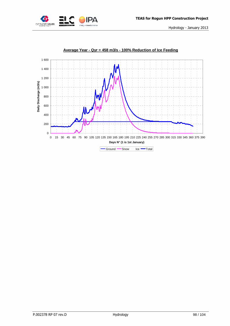
TEAS for Rogun HPP Construction Project
Hydrology - January 2013
P.002378 RP 07 rev.D Hydrology 98 / 104
Average Year - Qyr = 458 m3/s - 100% Reduction of I ce Feeding
0
200
400
600
800
1 000
1 200
1 400
1 600
0 15 30 45 60 75 90 105 120 135 150 165 180 195 210 225 240 255 270 285 300 315 330 345 360 375 390
Days N° (1 is 1st January)
Dai
ly D
isch
arge
(m
3/s)
Ground Snow Ice Total

TEAS for Rogun HPP Construction Project
Hydrology - January 2013
P.002378 RP 07 rev.D Hydrology 99 / 104
5.4 Scenario 2: Evolution of Discharges from 1990 t o 2100
After this specific study about the vanishing of glacier, an assessment of the evolution of
Vakhsh discharges was made by the Consultant under the assumption of a discharge
increasing trend (at same level as the historical trend of 0.8°C/century) associated to an ice
feeding reduction due to temperature increase as suggested by the Climate Models and
presented above. Two phenomenon were therefore coupled in this scenario: an ice feeding
reduction due to temperature rise and an increase in ground water contribution following the
historical trend.
The following Table 21 illustrates our results. The projections show that the ice feeding
contribution will weight in 2100, in the Vakhsh average discharge for 88 m3/s instead of
180 m3/s at the present time (i.e. 50% decrease of ice contribution). Conversely, assuming
the ground water contribution increase at the same level as historical trend, its contribution is
estimated in 2100 at 344 m3/s (i.e. 50% increase compared to actual ground water
contribution).
The impact of this two contribution evolution represents a clear diminution of maximum flood
in 2100. However the ground water increase contribution allows preserving a mean annual
flow as actual.
Note that a number of uncertainties affect the results:
• The 50% hypothesis for temperature increase might not be right
• The precipitation projections by climate models have such dispersion that the
no change option is the most prudent.
• Assuming a continuation of discharge trend might be right for the next 10 to
30 years and wrong on the long term.
• Knowledge of precipitation pattern is limited.
For operation study, a conservative assumption is to keep the present data set as it reflects
the glacier recession of past century.

TEAS for Rogun HPP Construction Project
Hydrology - January 2013
P.002378 RP 07 rev.D Hydrology 100 / 104
Table 21: Evolution of Discharges from 1990 to 2100
Item Present (1990) 2020 2050 2080 2100
Average (m3/s) 638 641 649 657 663 % 100 100,5 102 103 104 Daily Peak (m3/s) 2 600 2 500 2 100 1 910 1 790 % 100 96 81 74 69
Year Ground Snow Ice Total Qdmx 1 990 227 230 180 638 2 600 2 020 241 230 169 641 2 500 2 050 294 230 124 649 2 100 2 080 324 230 103 657 1 910 2 100 344 230 88 663 1 790
(m3/s)
Year 2020 - Average Year - Discharge Trend and Ice Feeding Reduction
0
500
1 000
1 500
2 000
2 500
3 000
0 15 30 45 60 75 90 105 120 135 150 165 180 195 210 225 240 255 270 285 300 315 330 345 360 375 390
Days N° (1 is 1st January)
Dai
ly D
isch
arge
(m
3/s)
Ground Snow Ice Total

TEAS for Rogun HPP Construction Project
Hydrology - January 2013
P.002378 RP 07 rev.D Hydrology 101 / 104
Year 2050 - Average Year - Discharge Trend and Ice Feeding Reduction
0
500
1 000
1 500
2 000
2 500
0 15 30 45 60 75 90 105 120 135 150 165 180 195 210 225 240 255 270 285 300 315 330 345 360 375 390
Days N° (1 is 1st January)
Dai
ly D
isch
arge
(m
3/s)
Ground Snow Ice Total
Year 2080 - Average Year - Discharge Trend and Ice Feeding Reduction
0
500
1 000
1 500
2 000
2 500
0 15 30 45 60 75 90 105 120 135 150 165 180 195 210 225 240 255 270 285 300 315 330 345 360 375 390
Days N° (1 is 1st January)
Dai
ly D
isch
arge
(m
3/s)
Ground Snow Ice Total

TEAS for Rogun HPP Construction Project
Hydrology - January 2013
P.002378 RP 07 rev.D Hydrology 102 / 104
Year 2100 - Average Year - Discharge Trend and Ice Feeding Reduction
0
200
400
600
800
1 000
1 200
1 400
1 600
1 800
2 000
0 15 30 45 60 75 90 105 120 135 150 165 180 195 210 225 240 255 270 285 300 315 330 345 360 375 390
Days N° (1 is January 1st)
Dai
ly D
isch
arge
(m
3/s)
Ground Snow Ice Total
Average Year - Comparison of Discharges from 1990 t o 2100
0
500
1 000
1 500
2 000
2 500
3 000
0 15 30 45 60 75 90 105 120 135 150 165 180 195 210 225 240 255 270 285 300 315 330 345 360 375 390
Days N° (1 is 1st January)
Dai
ly D
isch
arge
(m
3/s)
Present (1990) 2020 2050 2080 2100

TEAS for Rogun HPP Construction Project
Hydrology - January 2013
P.002378 RP 07 rev.D Hydrology 103 / 104
5.5 Climate Change and Adaptive Management:
5.5.1. Climate Change models as a tool to set up pr iorities:
Current Climate Change models give meaningful large scale projections that correlate with
long term physical observation of dramatic changes in climate, as for example glacier retreat.
These models are therefore excellent tools to set up adaption priorities as they already point
out major future impacts: changes in flow regimes on glacier melt driven rivers, changes in
seasonal discharge distribution, higher extreme event variability etc. These phenomena have
a large impact on hydropower facilities and should therefore be considered when planning
new projects as Rogun HPP.
However, as shown in the critical review of existing models on Climate Change in Central
Asia and in particular in Tajikistan and Amu-Darya basin, there is no doubt that further
research is required in order to reduce the uncertainties of the downscaled results, and make
them compatible with the level of accuracy required when designing a project as Rogun
HPP.
As on today, in particular in terms of precipitation patterns, trends provided by models, are
not accurate enough in order to try to understand the local impact of Climate Change on a
project as Rogun. Deriving adaptive measures in terms of design criteria based on the
current projections at a project level would be inappropriate. However, adaptation to climate
change must be incorporated in the overall planning of hydropower and irrigation
development in Central Asia.
The peculiarity of a project as Rogun is the transboundary aspect of water resources
competing with national interests, requiring integrated approach at a basin level for water use
(as already coordinated by ICWC and BVO Amudarya) but also for handling climate change
impacts on water regimes. Adaptation to Climate Change will require efficient use and
protection of water resources subject to new stresses, improving irrigation technologies for
better conservation of the resources and an international cooperation in the use of
hydropower resources at national and regional level.

TEAS for Rogun HPP Construction Project
Hydrology - January 2013
P.002378 RP 07 rev.D Hydrology 104 / 104
5.5.2. Adaptation measures to Climate Change:
Coping with Climate Change requires high level cooperation based on a step by step
approach:
• Reduce uncertainty: Research on climate change shall aim at better understanding
and modelling climate variations and allow accurate downscaling of results to derive
reliable trends on short as well as long term periods. This would allow incorporating
trends in the planning of facilities (design criteria) but also in the economic viability of
a project (inflow variability could be incorporated in financial and economic forecasts
for project viability).
• Reduce Vulnerability: Better understanding the potential threats would allow also
identifying the most vulnerable populations expected to be affected and incorporate
mitigation measures in the planning of projects (flood control etc.).
• Change use, location etc.: When such mitigation measures appear to be difficult or
non-viable to implement, then direct adjustment to human systems in response to
climatic stimuli shall be planned. This could also incorporate potential benefits from
climate change impacts as a change in economic opportunities.
• Adapt measures and inform: In the current status of knowledge, any measures
taken in order to cope with Climate Change are by essence, subject to adaptation on
the short term based on observations. Even a very robust and conservative design
shall allow some flexibility for updating to cope with the anticipated drastic changes.
This requires a strong observation network and environmental monitoring to be sure
to revise and renew adaptation measures as for example upgrade existing facilities.
This monitoring system could also strengthen weather forecast and early warning
system for minimization of natural disaster risks and increase preparedness to
extreme phenomena.
These key aspects are being brought up on the international scene for discussions at river
basin level to promote cooperation between countries that will be directly affected in quite a
short term horizon by Climate Change.