Embed Size (px)
Citation preview

SVEND HIPPS
Reliability Block Diagram
Markov Model – 2oo3 Voting
Master Thesis: Quantitative reliability modelling and functional safety calculations of
Svend topside High Integrity Pressure Protection System
Aalborg University Esbjerg
10th semester M.Sc. in Offshore Energy Systems – group OES10-2-F17
Jacob Glæsner
Printed June 8 th 2017

(This page is intentionally left blank)
10th semester master thesis Jacob Glæsner
Page | i
Project title: Master Thesis: Quantitative reliability modelling and functional safety calcu-
lations of Svend topside High Integrity Pressure Protection System
University: Aalborg University Esbjerg
Study program: Master of Science Programme in Sustainable Energy Engineering with
specialization in Offshore Energy Systems
Semester, group: 10th semester, OES10-2-F17
Semester theme: Master Thesis in Offshore Energy Systems
Project period: February 1st 2017 to June 8th 2017
ECTS: 30
Supervisor: Mohsen Soltani
Number of pages: 109 numbered pages, including appendix
Front page picture: Own creation
By signing this document or uploading it to the project data base each group member confirms to have
participated equally in the project and share the responsibility of the content of the report. In addition, all
group members confirm that plagiarism is not present in the report.
Jacob Glæsner
Title Page

10th semester master thesis Jacob Glæsner
Page | ii
(This page is intentionally left blank)
10th semester master thesis Jacob Glæsner
Page | iii
A conducted Layers Of Protection Analysis of Svend oil & gas platform predicted a hazardous incident to
cause up to 10 fatalities and up to 1000 MMUSD so an upgrade of the High Integrity Pressure Protection
System (HIPPS) was suggested. A HIPPS is a Safety Instrumented System that must have a certain level of
reliability in order to fulfill the required Safety Integrity Level (SIL) 2. The Svend HIPPS architecture and
different quantitative reliability methods i.e. Reliability Block Diagrams (RBD), Fault Tree Analysis (FTA) and
Markov modelling are described. Functional safety calculations i.e. the Probability of Failure on Demand
(PFDAvg) are performed with each method and compared. RBD and FTA are much similar in approach but
the complexity increases when using Markov modelling as the number of states may increase
exponentially. However, the SIS can be described more detailed with Markov modelling. The results of the
PFDAvg show a deviation within 1 % regardless of chosen method and the required SIL 2 is obtained with the
proposed components and architecture for Svend topside HIPPS. It is more important that the user of a
particular method is competent in using the chosen method than the method, which is actually used.
Abstract

10th semester master thesis Jacob Glæsner
Page | iv
(This page is intentionally left blank)

10th semester master thesis Jacob Glæsner
Page | v
During a 9th semester internship at Maersk Oil I worked with Safety Instrumented Systems (SIS) and particu-
larly installation of a High Integrity Pressure Protection System (HIPPS) at the unmanned Svend Platform –
see Chapter 3 page 15 for a more detailed description of the Svend platform and HIPPS. Installation of a
HIPPS is a long process with many considerations and calculations especially regarding safety. I was
introduced to reliability and functional safety calculations during the internship and concluded that it would
be a natural continuation of the internship to study this further in my master thesis.
This 10th semester master thesis is written by Jacob Glæsner as part of the M.Sc. in Offshore Energy
Systems study program at Aalborg University Esbjerg (AAUE). The master thesis is a continuation of the
work done in a 9th semester internship but with a dedicated focus on the reliability and functional safety of
the HIPPS and different means to calculate the reliability. In this context the thesis contains sections, which
would have been excluded in a commercial report.
The report is written in a language that requires prior knowledge to the Oil and Gas Industry. Even though
the Oil and Gas Industry is the foundation for this master thesis, reliability engineering is used in several
other industries. Relevant figures, tables and text from the 9th semester report will be included.
References to documentation and literature are placed in [brackets].
Used acronyms are explained in the text. A list of used acronyms can also be found at page xi.
Maersk Oil legends are used throughout the report. A list of used legends is provided at page xiii.
The PDF version of this report has bookmarks that ease navigation.
Special thanks are given to my supervisor Mohsen Soltani (assistant professor at AAUE) and colleagues at
Maersk Oil for technical assistance throughout the project period.
Preface

10th semester master thesis Jacob Glæsner
Page | vi
Title Page ............................................................................................ i
Abstract ............................................................................................ iii
Preface .............................................................................................. v
Table of Contents .............................................................................. vi
Abbreviations, Acronyms and Symbols ............................................. xi
Legends .......................................................................................... xiii
Introduction Section .......................................................................... 1
1 Scope of Thesis ............................................................................ 3
1.1 Motivation .............................................................................................................. 3
1.2 Objective ................................................................................................................ 3
1.3 Limitations .............................................................................................................. 4
Quantitative approaches .......................................................................................... 5 1.3.1
Modes of operation .................................................................................................. 6 1.3.2
Conclusion of limitations .......................................................................................... 6 1.3.3
1.4 Method ................................................................................................................... 6
1.5 Literature ................................................................................................................ 6
IEC and ISO standards ............................................................................................... 7 1.5.1
Maersk Oil documents .............................................................................................. 8 1.5.2
Books ........................................................................................................................ 8 1.5.3
Articles ...................................................................................................................... 9 1.5.4
1.6 State of the art Analysis ........................................................................................... 9
‘Reliability Engineering and Safety Systems’ Journal ............................................. 10 1.6.1
Other Articles .......................................................................................................... 10 1.6.2
1.7 Structure of the Report .......................................................................................... 11
Introduction Section ................................................................................................ 11 1.7.1
Modelling Section ................................................................................................... 11 1.7.2
Concluding Section .................................................................................................. 11 1.7.3
2 Safety Instrumented Systems .................................................... 12
2.1 Elements in SIS ...................................................................................................... 12
Sensors .................................................................................................................... 12 2.1.1
Table of Contents
10th semester master thesis Jacob Glæsner
Page | vii
Logic Solver ............................................................................................................. 12 2.1.2
Final Element .......................................................................................................... 13 2.1.3
Design principle – fail safe ...................................................................................... 13 2.1.4
2.2 Safety Instrumented Function ................................................................................ 13
2.3 Safety Integrity Level ............................................................................................. 13
3 Svend Platform & HIPPS Installation ......................................... 15
3.1 Equipment Under Control ...................................................................................... 16
3.2 HIPPS .................................................................................................................... 17
Current Svend HIPPS ............................................................................................... 17 3.2.1
Future HIPPS ........................................................................................................... 17 3.2.2
SIL requirement of future HIPPS ............................................................................. 18 3.2.3
Modelling Section ............................................................................. 21
4 Failure Modes ............................................................................. 23
4.1 No Effect Failure .................................................................................................... 23
4.2 Safe Failure ........................................................................................................... 23
4.3 Dangerous Failure ................................................................................................. 23
4.4 Failure Rate ........................................................................................................... 24
4.5 Common Cause Failure (CCF) ................................................................................. 25
𝜷-factor standard ................................................................................................... 25 4.5.1
𝜷-factor corrected .................................................................................................. 26 4.5.2
𝜷-factor – non-identical components ..................................................................... 27 4.5.3
4.6 Svend HIPPS Failure Modes ................................................................................... 28
5 Probability of Failure on Demand ............................................... 29
5.1 Definition of PFD ................................................................................................... 29
5.2 Requirements........................................................................................................ 30
5.3 PFD Formulas Relevant for Svend HIPPS ................................................................. 30
IEC 61508-6 Formulas ............................................................................................. 30 5.3.1
Simplified Formulas ................................................................................................ 31 5.3.2
CCF .......................................................................................................................... 32 5.3.3
5.4 Summary of Formulas ............................................................................................ 33
6 Reliability Block Diagrams .......................................................... 34
6.1 Assumptions and Definitions ................................................................................. 34

10th semester master thesis Jacob Glæsner
Page | viii
State of system ....................................................................................................... 34 6.1.1
State of components ............................................................................................... 34 6.1.2
6.2 Graphical & Mathematical Illustration of Boolean Logic [40] ................................... 35
Series structures ...................................................................................................... 35 6.2.1
Parallel structures and m out of n (moon) structures ............................................. 35 6.2.2
Other structures ...................................................................................................... 36 6.2.3
6.3 Probability Calculations ......................................................................................... 36
Constant probability of failure or success ............................................................... 37 6.3.1
MooN (non-identical components) IEC 11.8.2 ........................................................ 37 6.3.2
6.4 Svend HIPPS – RBD and PFD Calculations ............................................................... 38
Sensor subsystem.................................................................................................... 38 6.4.1
Logic Solver subsystem ........................................................................................... 39 6.4.2
Final Element subsystem ........................................................................................ 39 6.4.3
6.5 Table Determination ............................................................................................. 39
Table Analysis ......................................................................................................... 40 6.5.1
Summary ................................................................................................................. 42 6.5.2
6.6 Results of Svend HIPPS Calculations ....................................................................... 42
Article Comparison ................................................................................................. 43 6.6.1
7 Fault Tree Analysis [4] [3] [41] ................................................. 46
7.1 FTA Boolean Operators and Symbols ..................................................................... 47
Events...................................................................................................................... 48 7.1.1
7.2 FTA Mathematics .................................................................................................. 48
AND-gate ................................................................................................................ 48 7.2.1
OR-gate ................................................................................................................... 49 7.2.2
Minimal Cut Sets ..................................................................................................... 49 7.2.3
Average Probability of Failure on Demand ............................................................. 49 7.2.4
7.3 FTA of Svend HIPPS ............................................................................................... 50
Sensor Subsystem ................................................................................................... 50 7.3.1
Logic Solver Subsystem ........................................................................................... 51 7.3.2
Final Element Subsystem ........................................................................................ 52 7.3.3
7.4 Results: Svend HIPPS Basic Events .......................................................................... 52
8 Markov Modelling ....................................................................... 54
10th semester master thesis Jacob Glæsner
Page | ix
8.1 Basic Markov Modelling ........................................................................................ 54
8.2 Markov Mathematics ............................................................................................ 55
Kolmogorov Differential Equation [3] ..................................................................... 56 8.2.1
Time-dependent Solution ........................................................................................ 57 8.2.2
Steady State Solution .............................................................................................. 58 8.2.3
8.3 Results: Svend HIPPS – Markov Modelling .............................................................. 59
Sensor Subsystem ................................................................................................... 59 8.3.1
Logic Solver Subsystem ........................................................................................... 61 8.3.2
Final Element Subsystem ........................................................................................ 64 8.3.3
8.4 Summary of Results ............................................................................................... 65
9 Proof Test Interval ..................................................................... 67
9.1 Perfect Proof Testing ............................................................................................. 67
9.2 Imperfect Proof Testing ......................................................................................... 68
Concluding Section .......................................................................... 69
10 Conclusion .................................................................................. 71
10.1 SIS of Svend HIPPS ................................................................................................. 71
10.2 Comparison of RBD, FTA, and Markov Modelling .................................................... 72
10.3 Results of PFDAvg .................................................................................................... 73
10.4 Conclusive Summary ............................................................................................. 73
11 Bibliography ............................................................................... 74
12 Appendix .................................................................................... 79
12.1 Hazard Scenarios [42] ............................................................................................ 80
12.2 TMEL Values for existing installations [37] ............................................................. 81
12.3 Oil Group Classification [45] [46] ............................................................................ 82
12.4 Overall framework of IEC 61508 [47] ...................................................................... 84
12.5 Use of methods for general dependability analysis tasks [48] ................................. 85
12.6 Characteristic of selected dependability analysis method [48] ................................ 86
12.7 Inservice Inspection System Overall View............................................................... 87
12.8 DUC in the North Sea ............................................................................................. 88
12.9 Process Flow Diagram current HIPPS ...................................................................... 89
12.10 Process Flow Diagram future HIPPS [42] ................................................................. 91
12.11 PFD and SIL determination..................................................................................... 92

10th semester master thesis Jacob Glæsner
Page | x
Initiating Cause (IC)................................................................................................. 92 12.11.1
Independent Protection Layers (IPL) ....................................................................... 92 12.11.2
TMEL ....................................................................................................................... 92 12.11.3
Example of SIL determination of Safety Impact...................................................... 92 12.11.4
12.12 2oo3 Structure Function ........................................................................................ 93
Minimal Path Set .................................................................................................... 93 12.12.1
Minimal Cut Set ...................................................................................................... 93 12.12.2
12.13 moon non-identical components ........................................................................... 95
Boolean Truth Table................................................................................................ 95 12.13.1
Karnaugh Maps ...................................................................................................... 96 12.13.2
12.14 Taylor Series Expansion ......................................................................................... 98
12.15 MATLAB – PFD Table Determination ...................................................................... 99
12.16 MATLAB – Solving Time-Dependent Diff. Equations .............................................. 101
12.17 MATLAB – Solving Steady State Diff. Eqns. 2oo3 voting ........................................ 103
12.18 MATLAB – Solving Steady State Diff. Eqns. 1oo1 voting ........................................ 105
12.19 MATLAB – Solving Steady State Diff. Eqns. 1oo2 voting ........................................ 107
12.20 State Definition of a 2oo3 voting system .............................................................. 109
10th semester master thesis Jacob Glæsner
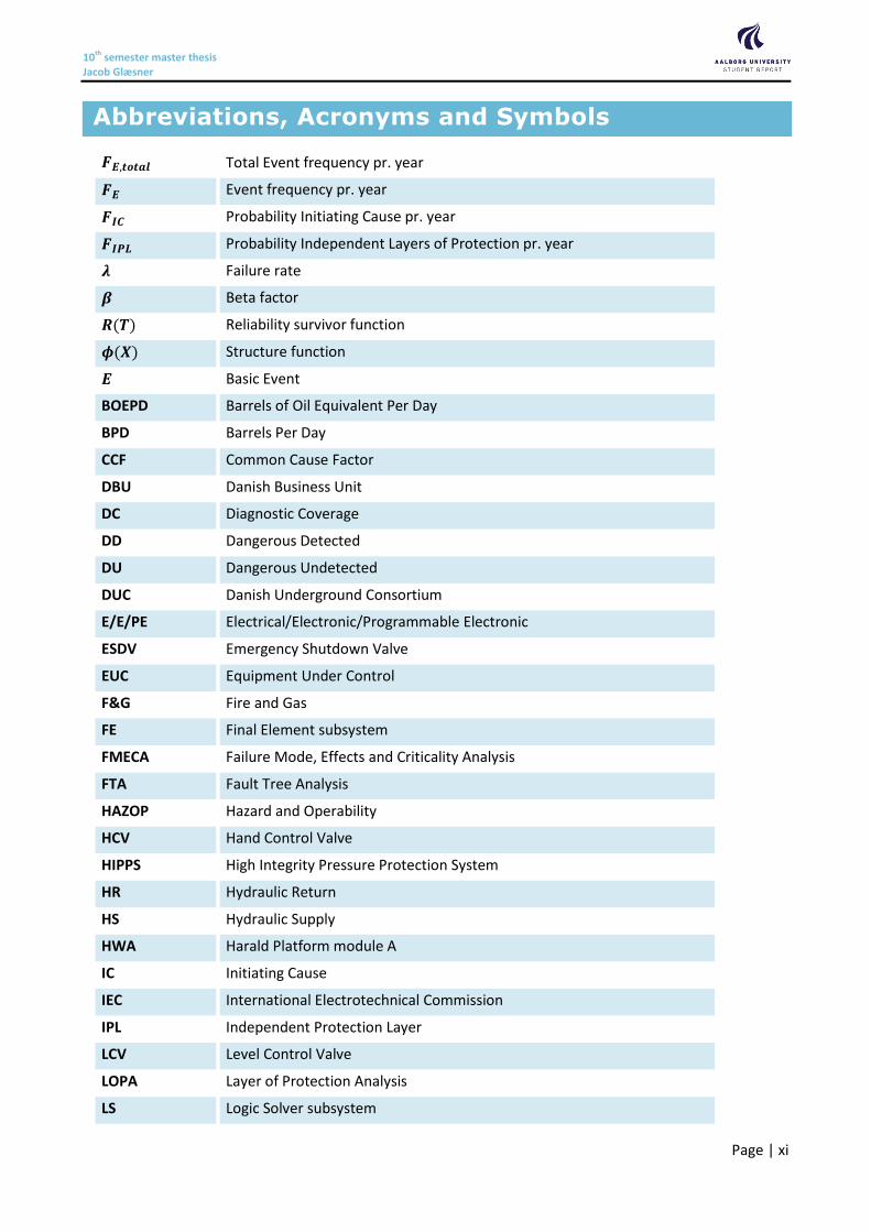
Page | xi
𝑭𝑬,𝒕𝒐𝒕𝒂𝒍 Total Event frequency pr. year
𝑭𝑬 Event frequency pr. year
𝑭𝑰𝑪 Probability Initiating Cause pr. year
𝑭𝑰𝑷𝑳 Probability Independent Layers of Protection pr. year
𝝀 Failure rate
𝜷 Beta factor
𝑹(𝑻) Reliability survivor function
𝝓(𝑿) Structure function
𝑬 Basic Event
BOEPD Barrels of Oil Equivalent Per Day
BPD Barrels Per Day
CCF Common Cause Factor
DBU Danish Business Unit
DC Diagnostic Coverage
DD Dangerous Detected
DU Dangerous Undetected
DUC Danish Underground Consortium
E/E/PE Electrical/Electronic/Programmable Electronic
ESDV Emergency Shutdown Valve
EUC Equipment Under Control
F&G Fire and Gas
FE Final Element subsystem
FMECA Failure Mode, Effects and Criticality Analysis
FTA Fault Tree Analysis
HAZOP Hazard and Operability
HCV Hand Control Valve
HIPPS High Integrity Pressure Protection System
HR Hydraulic Return
HS Hydraulic Supply
HWA Harald Platform module A
IC Initiating Cause
IEC International Electrotechnical Commission
IPL Independent Protection Layer
LCV Level Control Valve
LOPA Layer of Protection Analysis
LS Logic Solver subsystem
Abbreviations, Acronyms and Symbols
10th semester master thesis Jacob Glæsner
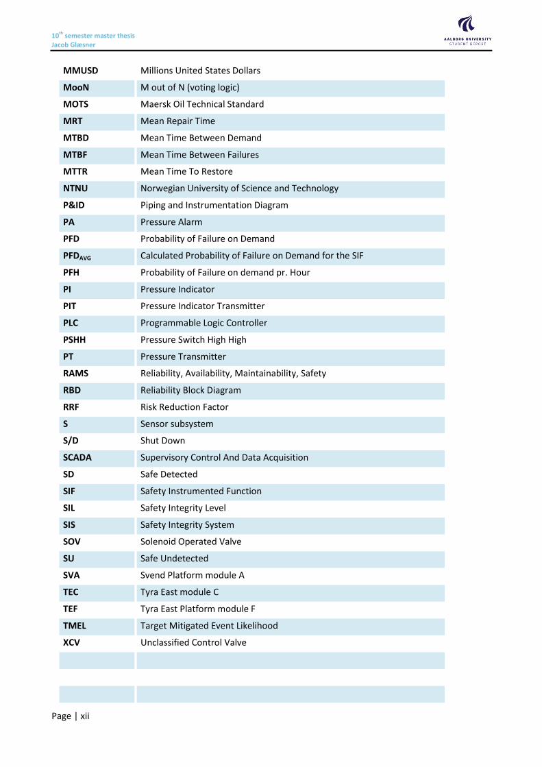
Page | xii
MMUSD Millions United States Dollars
MooN M out of N (voting logic)
MOTS Maersk Oil Technical Standard
MRT Mean Repair Time
MTBD Mean Time Between Demand
MTBF Mean Time Between Failures
MTTR Mean Time To Restore
NTNU Norwegian University of Science and Technology
P&ID Piping and Instrumentation Diagram
PA Pressure Alarm
PFD Probability of Failure on Demand
PFDAVG Calculated Probability of Failure on Demand for the SIF
PFH Probability of Failure on demand pr. Hour
PI Pressure Indicator
PIT Pressure Indicator Transmitter
PLC Programmable Logic Controller
PSHH Pressure Switch High High
PT Pressure Transmitter
RAMS Reliability, Availability, Maintainability, Safety
RBD Reliability Block Diagram
RRF Risk Reduction Factor
S Sensor subsystem
S/D Shut Down
SCADA Supervisory Control And Data Acquisition
SD Safe Detected
SIF Safety Instrumented Function
SIL Safety Integrity Level
SIS Safety Integrity System
SOV Solenoid Operated Valve
SU Safe Undetected
SVA Svend Platform module A
TEC Tyra East module C
TEF Tyra East Platform module F
TMEL Target Mitigated Event Likelihood
XCV Unclassified Control Valve
10th semester master thesis Jacob Glæsner
Page | xiii
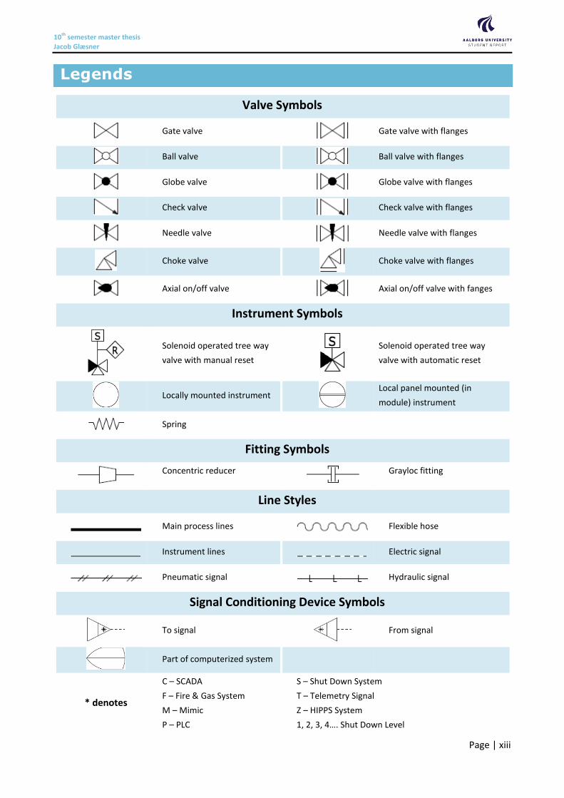
Valve Symbols
Gate valve
Gate valve with flanges
Ball valve
Ball valve with flanges
Globe valve
Globe valve with flanges
Check valve
Check valve with flanges
Needle valve
Needle valve with flanges
Choke valve
Choke valve with flanges
Axial on/off valve
Axial on/off valve with fanges
Instrument Symbols
Solenoid operated tree way
valve with manual reset
Solenoid operated tree way
valve with automatic reset
Locally mounted instrument
Local panel mounted (in
module) instrument
Spring
Fitting Symbols
Concentric reducer
Grayloc fitting
Line Styles
Main process lines Flexible hose
Instrument lines Electric signal
Pneumatic signal Hydraulic signal
Signal Conditioning Device Symbols
To signal
From signal
Part of computerized system
* denotes
C – SCADA
F – Fire & Gas System
M – Mimic
P – PLC
S – Shut Down System
T – Telemetry Signal
Z – HIPPS System
1, 2, 3, 4…. Shut Down Level
Legends

10th semester master thesis Jacob Glæsner
Page | xiv
(This page is intentionally left blank)
10th semester master thesis Jacob Glæsner
Page | 1
Introduction
Section

10th semester master thesis Jacob Glæsner
Page | 2
(This page is intentionally left blank)
10th semester master thesis Jacob Glæsner
Page | 3
1 Scope of Thesis
This chapter documents the motivation and objectives of the master thesis and method for documenting
and answering the objectives. Some concepts are just used and not elaborated in this chapter but will be
done in other chapters of the thesis.
1.1 Motivation
The reputation and performance of a company are measured by many different indicators e.g. quality,
safety, and reliability of products and services. A hazardous incident in a company may have safety,
environmental or commercial impact, which can damage the reputation and performance of the company
depending on the severity of the incident. A conducted Layers Of Protection Analysis (LOPA) at Maersk Oil
prior installation of a High Integrity Pressure Protection System (HIPPS) rated the severity of a hazardous
incident at the Svend platform. Prior to the LOPA different hazard scenarios regarding over pressurizing of
Svend were identified – see Appendix 12.1 page 80. During the LOPA a consequence assessment identified
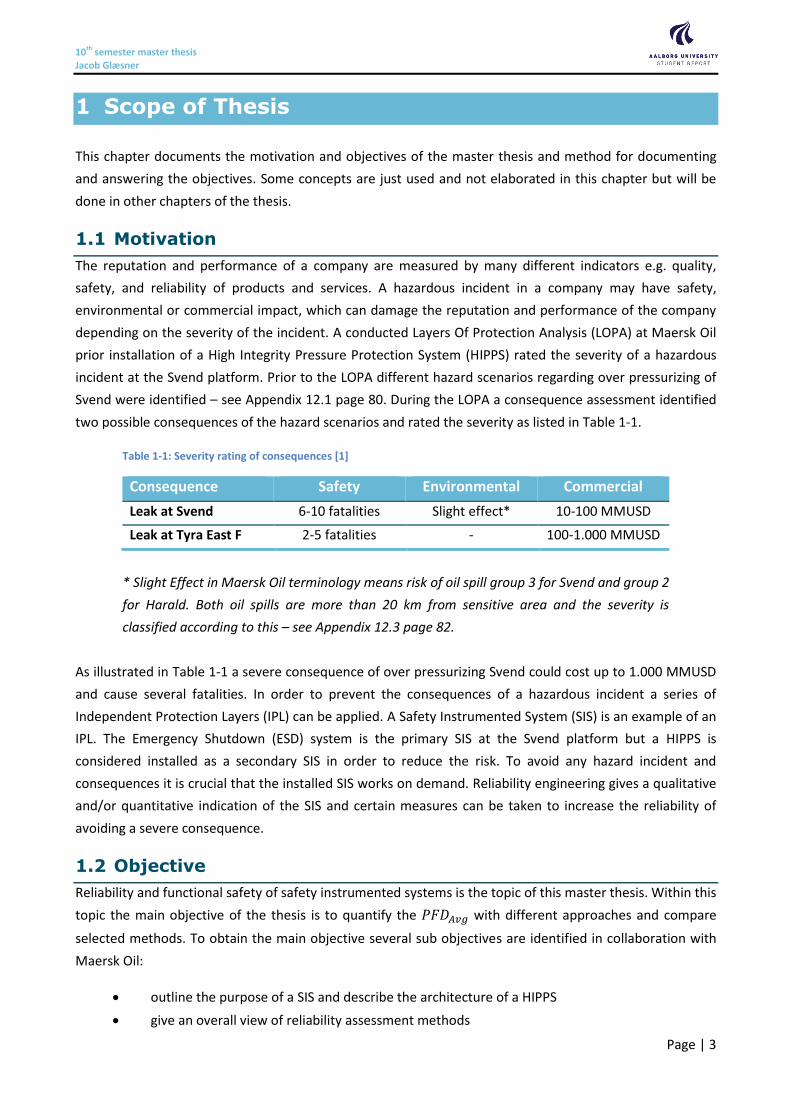
two possible consequences of the hazard scenarios and rated the severity as listed in Table 1-1.
Table 1-1: Severity rating of consequences [1]
Consequence Safety Environmental Commercial
Leak at Svend 6-10 fatalities Slight effect* 10-100 MMUSD
Leak at Tyra East F 2-5 fatalities - 100-1.000 MMUSD
* Slight Effect in Maersk Oil terminology means risk of oil spill group 3 for Svend and group 2
for Harald. Both oil spills are more than 20 km from sensitive area and the severity is
classified according to this – see Appendix 12.3 page 82.
As illustrated in Table 1-1 a severe consequence of over pressurizing Svend could cost up to 1.000 MMUSD
and cause several fatalities. In order to prevent the consequences of a hazardous incident a series of
Independent Protection Layers (IPL) can be applied. A Safety Instrumented System (SIS) is an example of an
IPL. The Emergency Shutdown (ESD) system is the primary SIS at the Svend platform but a HIPPS is
considered installed as a secondary SIS in order to reduce the risk. To avoid any hazard incident and
consequences it is crucial that the installed SIS works on demand. Reliability engineering gives a qualitative
and/or quantitative indication of the SIS and certain measures can be taken to increase the reliability of
avoiding a severe consequence.
1.2 Objective
Reliability and functional safety of safety instrumented systems is the topic of this master thesis. Within this
topic the main objective of the thesis is to quantify the 𝑃𝐹𝐷𝐴𝑣𝑔 with different approaches and compare
selected methods. To obtain the main objective several sub objectives are identified in collaboration with
Maersk Oil:
outline the purpose of a SIS and describe the architecture of a HIPPS
give an overall view of reliability assessment methods

10th semester master thesis Jacob Glæsner
Page | 4
discuss different approaches to determine and quantify reliability of a SIS
case study: analytical calculation of PFD, Availability, MTBF for Svend HIPPS
compare results of different quantitative methods – are there any difference?
does the calculated PFD fulfill the criteria of the Safety Integrity Level (SIL) analysis?
illustrate the impact on PFD in changing the test interval of HIPPS instrumentation
use relevant literature and recent research in the analysis
1.3 Limitations
Reliability analysis is a subpart of risk management as illustrated in Figure 1-1. Within reliability analysis
different qualitative, quantitative, and semi-quantitative approaches can be used as outlined in Appendix
12.5 page 85 and Appendix 12.6 page 86. The objective of this thesis is to give a quantitative result of the
reliability analysis with different modelling techniques and calculations, so qualitative approaches will not
be considered.
Figure 1-1: Framework of risk management [2]
Reliability analysis consists of three main branches:
Hardware reliability
Reliability of technical components and systems can be divided into two approaches:
Physical – Will not be part of this thesis as it is mainly used for reliability analysis of
structural elements and assessment of loads and stresses.
Actuarial – Main focus in this thesis as it applicable to components and systems.
Software reliability
Will not be treated in this master thesis due to the fact that this is not required to claim
compliance with IEC 61508 and will often be performed by software specialists. [3]
Human reliability
Though many technical components also involve human interactions it will not be a topic in
this thesis. Whenever human interaction is required in calculations their interactions are
considered 100 % reliable.
10th semester master thesis Jacob Glæsner
Page | 5
Quantitative approaches 1.3.1
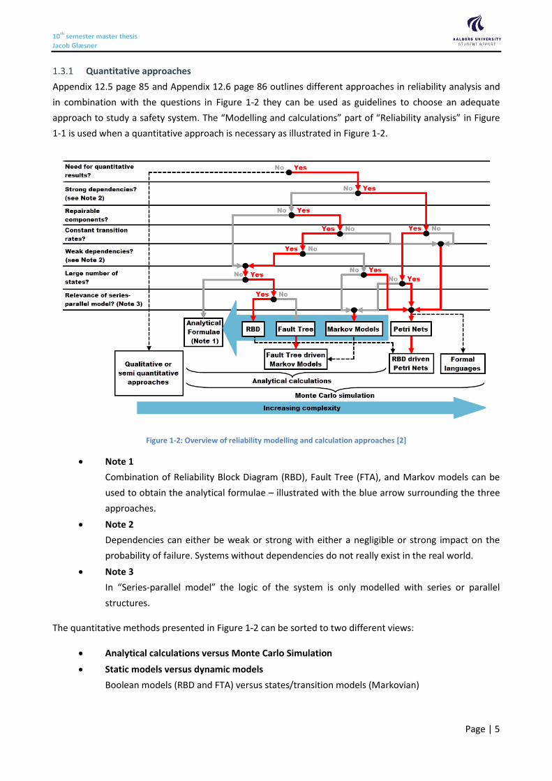
Appendix 12.5 page 85 and Appendix 12.6 page 86 outlines different approaches in reliability analysis and
in combination with the questions in Figure 1-2 they can be used as guidelines to choose an adequate
approach to study a safety system. The “Modelling and calculations” part of “Reliability analysis” in Figure
1-1 is used when a quantitative approach is necessary as illustrated in Figure 1-2.
Figure 1-2: Overview of reliability modelling and calculation approaches [2]
Note 1
Combination of Reliability Block Diagram (RBD), Fault Tree (FTA), and Markov models can be
used to obtain the analytical formulae – illustrated with the blue arrow surrounding the three
approaches.
Note 2
Dependencies can either be weak or strong with either a negligible or strong impact on the
probability of failure. Systems without dependencies do not really exist in the real world.
Note 3
In “Series-parallel model” the logic of the system is only modelled with series or parallel
structures.
The quantitative methods presented in Figure 1-2 can be sorted to two different views:
Analytical calculations versus Monte Carlo Simulation
Static models versus dynamic models
Boolean models (RBD and FTA) versus states/transition models (Markovian)
10th semester master thesis Jacob Glæsner
Page | 6
According to IEC 61508 the choice of method is less important than the user’s competence in using a
specific method:
“All these methods can be used for the majority of safety related systems and, when deciding
which technique to use on any particular application, it is very important that the user of a
particular technique is competent in using the technique and this may be more important than
the technique which is actually used….” [4]
Modes of operation 1.3.2
The mode of operation of a Safety Instrumented Function (SIF) is categorized according to how often the
function is demanded. IEC 61508 defines three different modes of operation.
Low-demand mode
Mean Time Between Demand (MTBD) > 1 year
High-demand mode
MTBD < 1 year
Continuous mode
Operates continuously and may be defined as a special case of high-demand mode
The main difference between a SIF in continuous mode and demand mode is that a SIF in continuous mode
plays an active role in protecting the Equipment Under Control (EUC), while a SIF in demand mode is
passive and will only operate when needed. IEC 61508 combines high-demand mode and continuous mode
into one mode called “high-demand mode/continuous mode” [4]. IEC 61511 only distinguishes between
demand mode and continuous mode [5]. A SIS can perform more than one SIF, so practically a SIS will be
able to operate in low demand mode and high-demand mode.
Conclusion of limitations 1.3.3
Based on these considerations the thesis will be limited to quantitative analytical calculations of the
reliability of Svend HIPPS with special focus on RBD, FTA, and Markov Model analysis. Svend HIPPS is
defined to operate in low-demand mode of operation with a MTBD > 1 year.
1.4 Method
A literature review of books and research articles is used to describe the concepts of reliability analysis and
safety instrumented systems. Analytical calculations of a case-study of Svend HIPPS will be performed after
a literature review of RBD, FTA, and Markov Modelling.
1.5 Literature
The master thesis is based on a literature review of international IEC and ISO standards and reports, and
internal Maersk Oil documents and standards. Some of the listed literature in the bibliography is only used
as background knowledge and not referenced in the thesis. The comprehensive bibliography is established
by a broad search on the reliability topic. Relevant literature was selected and their references used for
further literature search. Multiple references of the chosen literature were used as a quality mark of the
chosen literature.
10th semester master thesis Jacob Glæsner
Page | 7
IEC and ISO standards 1.5.1
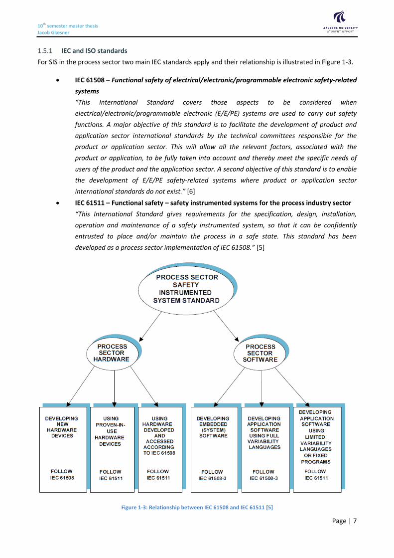
For SIS in the process sector two main IEC standards apply and their relationship is illustrated in Figure 1-3.
IEC 61508 – Functional safety of electrical/electronic/programmable electronic safety-related
systems
“This International Standard covers those aspects to be considered when
electrical/electronic/programmable electronic (E/E/PE) systems are used to carry out safety
functions. A major objective of this standard is to facilitate the development of product and
application sector international standards by the technical committees responsible for the
product or application sector. This will allow all the relevant factors, associated with the
product or application, to be fully taken into account and thereby meet the specific needs of
users of the product and the application sector. A second objective of this standard is to enable
the development of E/E/PE safety-related systems where product or application sector
international standards do not exist.” [6]
IEC 61511 – Functional safety – safety instrumented systems for the process industry sector
“This International Standard gives requirements for the specification, design, installation,
operation and maintenance of a safety instrumented system, so that it can be confidently
entrusted to place and/or maintain the process in a safe state. This standard has been
developed as a process sector implementation of IEC 61508.” [5]
Figure 1-3: Relationship between IEC 61508 and IEC 61511 [5]

10th semester master thesis Jacob Glæsner
Page | 8
According to Figure 1-3 Maersk Oil must follow IEC 61511 as an operator while vendors must follow IEC
61508. In this master thesis the main focus will be on IEC 61508 because IEC 61511 gives a more general
view on how to implement SIS. Appendix 12.4 page 84 gives an overall view of the framework of IEC 61508
– especially IEC 61508-6 is used as it gives guidelines to relevant reliability methods.
Other important used standards and technical reports include:
IEC 60300-3-1 – Dependability management – Part 3-1: Application guide – Analysis
techniques for dependability – Guide on methodology
IEC 61025 – Fault tree analysis (FTA)
IEC 61078 – Reliability block diagrams
IEC 61165 – Application of Markov techniques
IEC 61703 – Mathematical expressions for reliability, availability, maintainability and
maintenance support terms
ISO/TR 12489 – Petroleum, petrochemical and natural gas industries – Reliability modelling
and calculation of safety systems
The bibliography contains more standards and technical reports used as background literature.
Maersk Oil documents 1.5.2
Internal Maersk Oil documents have been used including:
Maersk Oil Technical Standards (MOTS)
Guidelines and Instructions
Standards
P&ID and Technical drawings
Reports
Vendor documentation
Standards, guidelines, and instruction are based on IEC standards.
No further detailed description of Maersk Oil internal documents.
Books 1.5.3
Different views of certain topics are provided by different authors. The main authors and books used for
this thesis are cited and referenced in used IEC standards and articles:
Birolini, Alessandro
“Reliability Engineering: Theory and Practice” [7]
Goble, William
“Control Systems Safety Evaluation and Reliability” [8]
Rausand, Marvin
“System Reliability Theory: Models, Statistical Methods, and Applications” [9]
“Reliability of Safety-Critical Systems: Theory and Applications” [3]
“Risk Assessment: Theory, Methods, and Applications” [10]

10th semester master thesis Jacob Glæsner
Page | 9
Zio, Enrico
”An Introduction to the Basics of Reliability and Risk Analysis” [11]
“Computational Methods for Reliability and Risk Analysis” [12]
“Basics of Reliability and Risk Analysis Worked Out Problems and Solutions” [13]
Other books are used as supplementary literature.
Reliability data books with collected industry data are used for Reliability, Availability, Maintenance, and
Safety (RAMS) analysis.
SINTEF – OREDA-2009
“Offshore Reliability Data Handbook: Volume 1 - Topside Equipment” [14]
SINTEF
“Reliability Data for Safety Instrumented Systems – PDS Data Handbook” [15]
SINTEF is a large independent research organization in Scandinavia, which has prepared the Offshore &
onshore REliability DAta (OREDA) handbook. OREDA is a project organization sponsored by eight worldwide
oil and gas companies: BP, Total, Statoil, Petrobas, Shell, EN, ENI, Gassco. OREDA’s main purpose is to
collect and exchange reliability data between the participating companies. [14]
Articles 1.5.4
Many different articles within the topic of reliability analysis regarding RBD, Fault Tree, and Markov
Analysis have been assessed to gain insight in recent research. The used articles will be cited when
necessary.
A further review of articles will be given in Section 1.6 – State of the art Analysis.
1.6 State of the art Analysis
The topic of reliability assessment has attracted a lot of research interests and this section will introduce
the articles used in this thesis.
The used articles are chosen from the following criteria:
Article relevance to subject of this thesis
The used articles are chosen within the following subject: SIL, PFD, RBD, FTA, Markov
Modelling, MooN structures, and proof testing and failures.
Journal
The ‘Reliability Engineering and Safety Systems’ journal is the main contributor of articles used
in this thesis but other articles have been used if they were found valid and relevant.
Author of articles
The first gross selection of articles was filtered on author and only authors, which had many
citations or publications of either articles or books were selected e.g. Rausand (a contributor of
books used in this thesis – see Section 1.5.3 page 8.
10th semester master thesis Jacob Glæsner
Page | 10
Citations of articles
The articles were also chosen with respect to the number of citations in other articles e.g. how
many times have someone else cited the article.
‘Reliability Engineering and Safety Systems’ Journal 1.6.1
The journal is the main contributor of articles used in this thesis. It is published by Elsevier in association
with the European Safety and Reliability Association, and the Safety Engineering and Risk Analysis Division.
The journal is an international journal devoted to development and application of methods in order to
enhance the safety and reliability of complex technological systems, including offshore systems. Normally it
only publishes articles that involve the analysis of substantive problems related to reliability of complex
systems. An important aim of the journal is to achieve a balance between practical applications and
academic material. The validity of the articles in the journal is considered high because of the criteria in
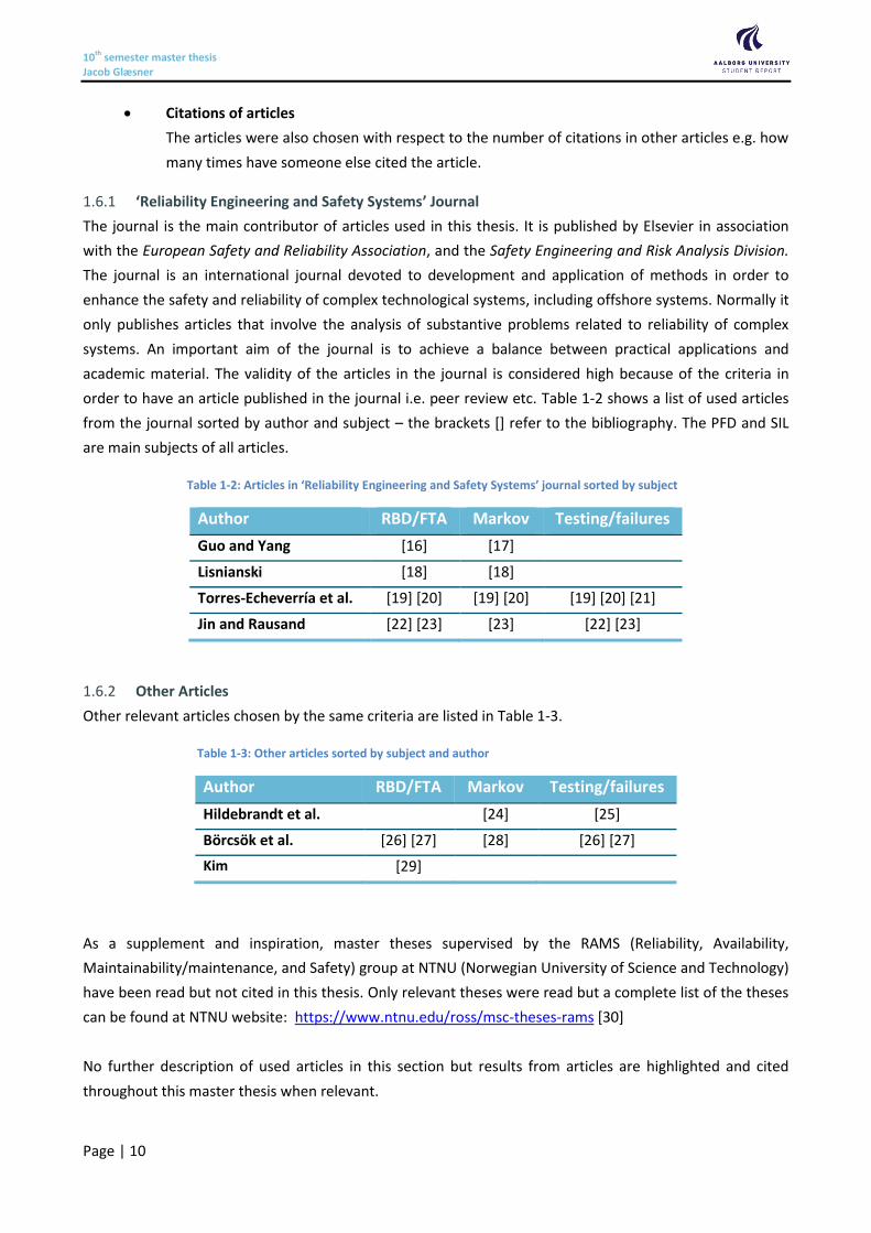
order to have an article published in the journal i.e. peer review etc. Table 1-2 shows a list of used articles
from the journal sorted by author and subject – the brackets [] refer to the bibliography. The PFD and SIL
are main subjects of all articles.
Table 1-2: Articles in ‘Reliability Engineering and Safety Systems’ journal sorted by subject
Author RBD/FTA Markov Testing/failures
Guo and Yang [16] [17]
Lisnianski [18] [18]
Torres-Echeverría et al. [19] [20] [19] [20] [19] [20] [21]
Jin and Rausand [22] [23] [23] [22] [23]
Other Articles 1.6.2
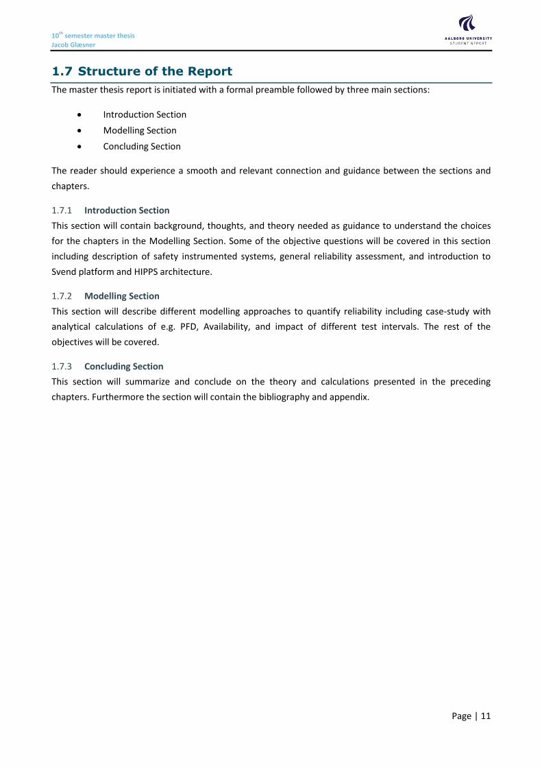
Other relevant articles chosen by the same criteria are listed in Table 1-3.
Table 1-3: Other articles sorted by subject and author
Author RBD/FTA Markov Testing/failures
Hildebrandt et al. [24] [25]
Börcsök et al. [26] [27] [28] [26] [27]
Kim [29]
As a supplement and inspiration, master theses supervised by the RAMS (Reliability, Availability,
Maintainability/maintenance, and Safety) group at NTNU (Norwegian University of Science and Technology)
have been read but not cited in this thesis. Only relevant theses were read but a complete list of the theses
can be found at NTNU website: https://www.ntnu.edu/ross/msc-theses-rams [30]
No further description of used articles in this section but results from articles are highlighted and cited
throughout this master thesis when relevant.
10th semester master thesis Jacob Glæsner
Page | 11
1.7 Structure of the Report
The master thesis report is initiated with a formal preamble followed by three main sections:
Introduction Section
Modelling Section
Concluding Section
The reader should experience a smooth and relevant connection and guidance between the sections and
chapters.
Introduction Section 1.7.1
This section will contain background, thoughts, and theory needed as guidance to understand the choices
for the chapters in the Modelling Section. Some of the objective questions will be covered in this section
including description of safety instrumented systems, general reliability assessment, and introduction to
Svend platform and HIPPS architecture.
Modelling Section 1.7.2
This section will describe different modelling approaches to quantify reliability including case-study with
analytical calculations of e.g. PFD, Availability, and impact of different test intervals. The rest of the
objectives will be covered.
Concluding Section 1.7.3
This section will summarize and conclude on the theory and calculations presented in the preceding
chapters. Furthermore the section will contain the bibliography and appendix.
10th semester master thesis Jacob Glæsner
Page | 12
2 Safety Instrumented Systems
Safety Instrumented Systems (SIS) have been used in the process sector, and especially the oil and gas
industry, for many years as a protection layer to protect the Equipment Under Control (EUC) against
hazardous incidents. Examples of SIS in the oil and gas industry and process sector:
PSD – Process Shutdown system
ESD – Emergency Shutdown system
HIP(P)S – High Integrity Protection System (e.g. against pressure (P), temperature, level etc.)
F&G – Fire & Gas detection system
A SIS may perform one or more Safety Instrumented Functions (SIF) – see Section 2.2.
IEC 61511 and IEC 61508 are the standards that address the application of SIS for the oil and gas industry,
which are based on the use of electrical/electronic/ programmable electronic (E/EP/PE) technology.
2.1 Elements in SIS
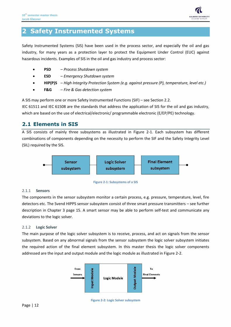
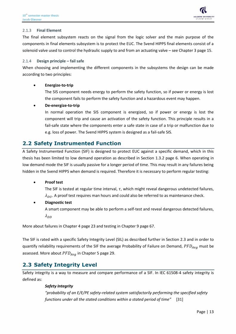
A SIS consists of mainly three subsystems as illustrated in Figure 2-1. Each subsystem has different
combinations of components depending on the necessity to perform the SIF and the Safety Integrity Level
(SIL) required by the SIS.
Figure 2-1: Subsystems of a SIS
Sensors 2.1.1
The components in the sensor subsystem monitor a certain process, e.g. pressure, temperature, level, fire
detectors etc. The Svend HIPPS sensor subsystem consist of three smart pressure transmitters – see further
description in Chapter 3 page 15. A smart sensor may be able to perform self-test and communicate any
deviations to the logic solver.
Logic Solver 2.1.2
The main purpose of the logic solver subsystem is to receive, process, and act on signals from the sensor
subsystem. Based on any abnormal signals from the sensor subsystem the logic solver subsystem initiates
the required action of the final element subsystem. In this master thesis the logic solver components
addressed are the input and output module and the logic module as illustrated in Figure 2-2.
Figure 2-2: Logic Solver subsystem
10th semester master thesis Jacob Glæsner
Page | 13
Final Element 2.1.3
The final element subsystem reacts on the signal from the logic solver and the main purpose of the
components in final elements subsystem is to protect the EUC. The Svend HIPPS final elements consist of a
solenoid valve used to control the hydraulic supply to and from an actuating valve – see Chapter 3 page 15.
Design principle – fail safe 2.1.4
When choosing and implementing the different components in the subsystems the design can be made
according to two principles:
Energize-to-trip
The SIS component needs energy to perform the safety function, so if power or energy is lost
the component fails to perform the safety function and a hazardous event may happen.
De-energize-to-trip
In normal operation the SIS component is energized, so if power or energy is lost the
component will trip and cause an activation of the safety function. This principle results in a
fail-safe state where the components enter a safe state in case of a trip or malfunction due to
e.g. loss of power. The Svend HIPPS system is designed as a fail-safe SIS.
2.2 Safety Instrumented Function
A Safety Instrumented Function (SIF) is designed to protect EUC against a specific demand, which in this
thesis has been limited to low demand operation as described in Section 1.3.2 page 6. When operating in
low demand mode the SIF is usually passive for a longer period of time. This may result in any failures being
hidden in the Svend HIPPS when demand is required. Therefore it is necessary to perform regular testing:
Proof test
The SIF is tested at regular time interval, 𝜏, which might reveal dangerous undetected failures,
𝜆𝐷𝑈. A proof test requires man hours and could also be referred to as maintenance check.
Diagnostic test
A smart component may be able to perform a self-test and reveal dangerous detected failures,
𝜆𝐷𝐷
More about failures in Chapter 4 page 23 and testing in Chapter 9 page 67.
The SIF is rated with a specific Safety Integrity Level (SIL) as described further in Section 2.3 and in order to
quantify reliability requirements of the SIF the average Probability of Failure on Demand, 𝑃𝐹𝐷𝐴𝑣𝑔 must be
assessed. More about 𝑃𝐹𝐷𝐴𝑣𝑔 in Chapter 5 page 29.
2.3 Safety Integrity Level
Safety integrity is a way to measure and compare performance of a SIF. In IEC 61508-4 safety integrity is
defined as:
Safety Integrity
“probability of an E/E/PE safety-related system satisfactorily performing the specified safety
functions under all the stated conditions within a stated period of time” [31]
10th semester master thesis Jacob Glæsner
Page | 14
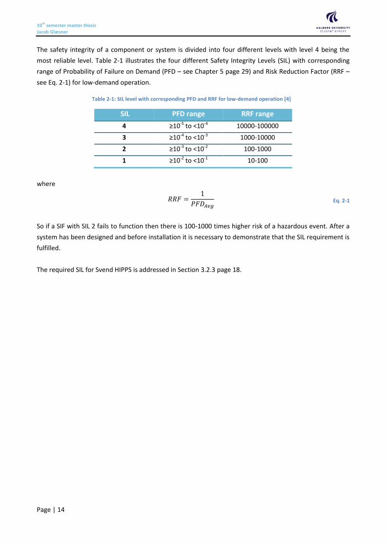
The safety integrity of a component or system is divided into four different levels with level 4 being the
most reliable level. Table 2-1 illustrates the four different Safety Integrity Levels (SIL) with corresponding
range of Probability of Failure on Demand (PFD – see Chapter 5 page 29) and Risk Reduction Factor (RRF –
see Eq. 2-1) for low-demand operation.
Table 2-1: SIL level with corresponding PFD and RRF for low-demand operation [4]
SIL PFD range RRF range
4 ≥10-5 to <10-4 10000-100000
3 ≥10-4 to <10-3 1000-10000
2 ≥10-3 to <10-2 100-1000
1 ≥10-2 to <10-1 10-100
where
𝑅𝑅𝐹 =1
𝑃𝐹𝐷𝐴𝑣𝑔 Eq. 2-1
So if a SIF with SIL 2 fails to function then there is 100-1000 times higher risk of a hazardous event. After a
system has been designed and before installation it is necessary to demonstrate that the SIL requirement is
fulfilled.
The required SIL for Svend HIPPS is addressed in Section 3.2.3 page 18.
10th semester master thesis Jacob Glæsner
Page | 15
3 Svend Platform & HIPPS Installation
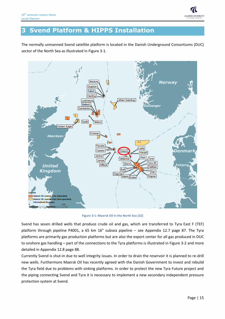
The normally unmanned Svend satellite platform is located in the Danish Underground Consortiums (DUC)
sector of the North Sea as illustrated in Figure 3-1.
Figure 3-1: Maersk Oil in the North Sea [32]
Svend has seven drilled wells that produce crude oil and gas, which are transferred to Tyra East F (TEF)
platform through pipeline P4001, a 65 km 16” subsea pipeline – see Appendix 12.7 page 87. The Tyra
platforms are primarily gas production platforms but are also the export center for all gas produced in DUC
to onshore gas handling – part of the connections to the Tyra platforms is illustrated in Figure 3-2 and more
detailed in Appendix 12.8 page 88.
Currently Svend is shut-in due to well integrity issues. In order to drain the reservoir it is planned to re-drill
new wells. Furthermore Maersk Oil has recently agreed with the Danish Government to invest and rebuild
the Tyra field due to problems with sinking platforms. In order to protect the new Tyra Future project and
the piping connecting Svend and Tyra it is necessary to implement a new secondary independent pressure
protection system at Svend.
10th semester master thesis Jacob Glæsner
Page | 16
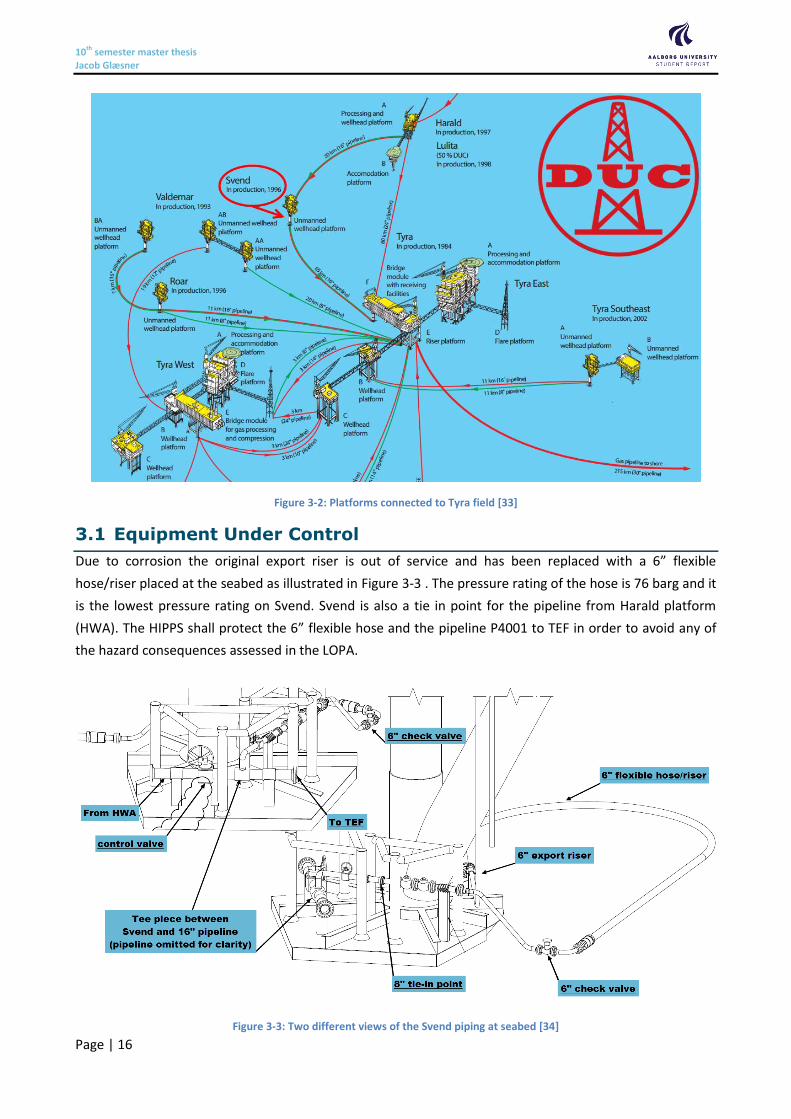
Figure 3-2: Platforms connected to Tyra field [33]
3.1 Equipment Under Control
Due to corrosion the original export riser is out of service and has been replaced with a 6” flexible
hose/riser placed at the seabed as illustrated in Figure 3-3 . The pressure rating of the hose is 76 barg and it
is the lowest pressure rating on Svend. Svend is also a tie in point for the pipeline from Harald platform
(HWA). The HIPPS shall protect the 6” flexible hose and the pipeline P4001 to TEF in order to avoid any of
the hazard consequences assessed in the LOPA.
Figure 3-3: Two different views of the Svend piping at seabed [34]
10th semester master thesis Jacob Glæsner
Page | 17
3.2 HIPPS
Current Svend HIPPS 3.2.1
The current primary Emergency Shutdown (ESD) system is upgraded with extra sensors and final elements
and is internally in Maersk Oil called a 1st generation High Integrity Pressure Protection System (HIPPS).
According to international standards IEC61508/11 the current HIPPS does not fulfill the criteria of a HIPPS
because it is not independent of the primary ESD protection system [35]. The two systems share sensors
and final elements and an upgrade is needed. Table 3-1 lists the EUC of the current 1st generation HIPPS.
See connection between EUC and SIS in Appendix 12.9 page 89.
Table 3-1: Equipment Under Control (EUC) and HIPPS components
EUC Design Pressure Sensors Logic Solver Final Elements
6” flexible hose/riser and
16” subsea pipeline, P-
4001
76 barg SVA-PT-30X09
SVA-SOV-30X03
SVA-WCV-30X03
SVA-PT-33004/5
SVA-PSHH-33008
SVA.FP-2201 SVA-SOV-33010
SVA-ESDV-33010
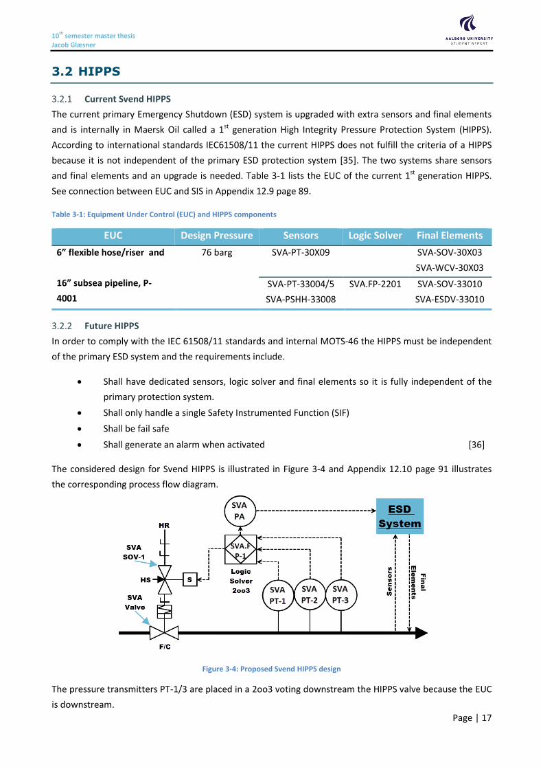
Future HIPPS 3.2.2
In order to comply with the IEC 61508/11 standards and internal MOTS-46 the HIPPS must be independent
of the primary ESD system and the requirements include.
Shall have dedicated sensors, logic solver and final elements so it is fully independent of the
primary protection system.
Shall only handle a single Safety Instrumented Function (SIF)
Shall be fail safe
Shall generate an alarm when activated [36]
The considered design for Svend HIPPS is illustrated in Figure 3-4 and Appendix 12.10 page 91 illustrates
the corresponding process flow diagram.
Figure 3-4: Proposed Svend HIPPS design
The pressure transmitters PT-1/3 are placed in a 2oo3 voting downstream the HIPPS valve because the EUC
is downstream.
10th semester master thesis Jacob Glæsner
Page | 18
SIL requirement of future HIPPS 3.2.3
In the performed LOPA a semi-quantitative assessment of the PFD was performed using the Independent
Protection Layers (IPL) to reduce the event frequency (𝐹𝐸) risk of the different Initiating Causes (IC). The
probabilities of each IPL can be calculated or assessed in Maersk Oil “Standard - Safety Integrity Level (SIL)
Analysis” [37]. See Appendix 12.11 page 92 for used IC and IPL.
The event frequency pr. year (𝐹𝐸) for each IC is calculated by multiplying the probability of the IC, 𝐹𝐼𝐶with
each of the probabilities of the IPLs (𝐹𝐼𝑃𝐿) – as illustrated in Eq. 3-1.
𝐹𝐸 = 𝐹𝐼𝐶 × ∏𝐹𝐼𝑃𝐿,𝑗
𝑛
𝑗=1
Eq. 3-1
The total event frequency pr. year (𝐹𝐸,𝑡𝑜𝑡𝑎𝑙) is the sum of 𝐹𝐸 for each IC – as illustrated in Eq. 3-2.
𝐹𝐸,𝑡𝑜𝑡𝑎𝑙 = ∑ (𝐹𝐼𝐶,𝑘 × ∏𝐹𝐼𝑃𝐿,𝑗
𝑛
𝑗=1
)
𝑚
𝑘=1
Eq. 3-2
where
𝑚 = 𝑛𝑢𝑚𝑏𝑒𝑟 𝑜𝑓 𝐼𝐶𝑠
𝑛 = 𝑛𝑢𝑚𝑏𝑒𝑟 𝑜𝑓 𝐼𝑃𝐿𝑠
The severity of each consequence presented in Table 1-1 page 3 has a Target Mitigated Event Likelihood
(TMEL) value as seen in Appendix 12.2 page 81. The TMEL is used in calculating the 𝑃𝐹𝐷 for each of the
different assessed consequences and associated Safety, Environmental and Commercial Impact – as
illustrated in Eq. 3-3. [4]
𝑃𝐹𝐷𝑎𝑣𝑔 =𝑇𝑀𝐸𝐿
𝐹𝐸,𝑡𝑜𝑡𝑎𝑙 Eq. 3-3
An example of SIL determination for Safety Impact of the consequence regarding over pressure at the
Svend platform is illustrated in Table 12-1, Appendix 12.11 page 92.
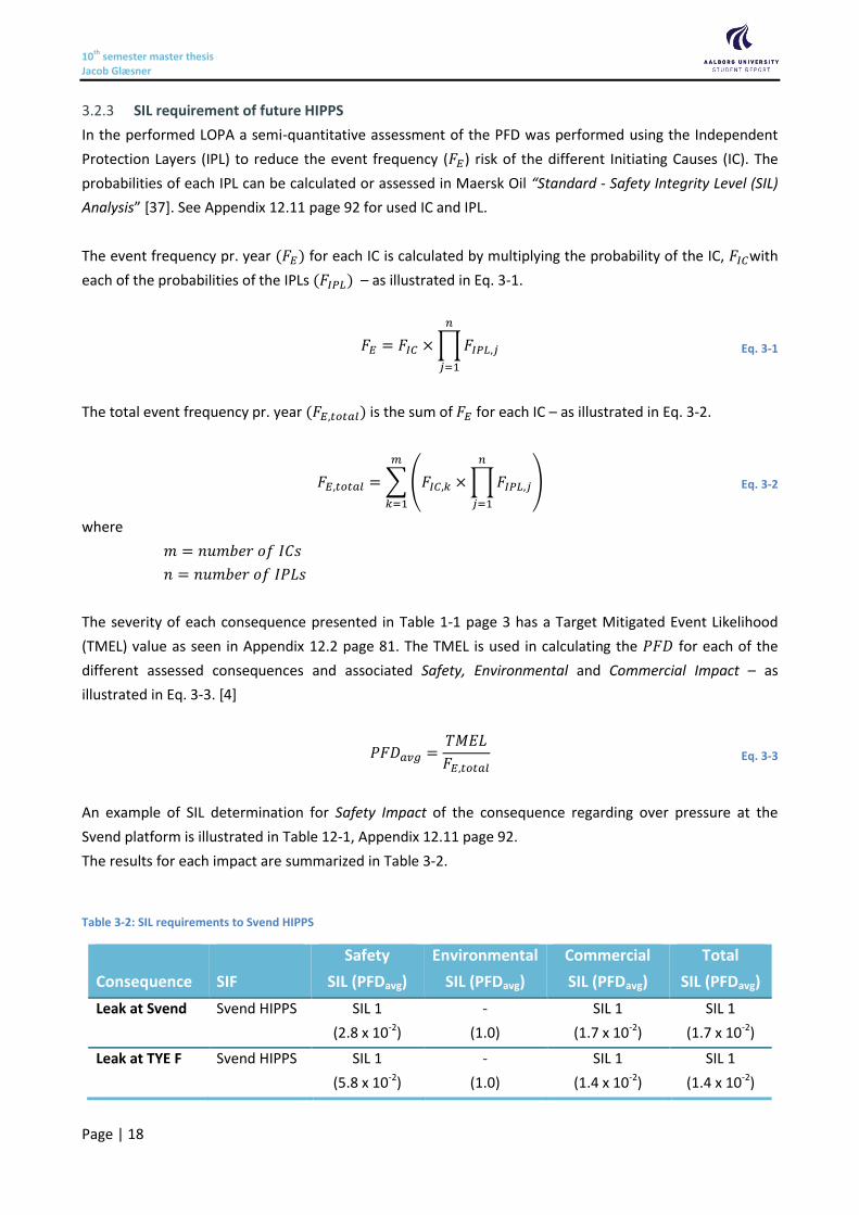
The results for each impact are summarized in Table 3-2.
Table 3-2: SIL requirements to Svend HIPPS
Consequence
SIF
Safety
SIL (PFDavg)
Environmental
SIL (PFDavg)
Commercial
SIL (PFDavg)
Total
SIL (PFDavg)
Leak at Svend Svend HIPPS SIL 1
(2.8 x 10⁻²)
-
(1.0)
SIL 1
(1.7 x 10⁻²)
SIL 1
(1.7 x 10⁻²)
Leak at TYE F Svend HIPPS SIL 1
(5.8 x 10⁻²)
-
(1.0)
SIL 1
(1.4 x 10⁻²)
SIL 1
(1.4 x 10⁻²)

10th semester master thesis Jacob Glæsner
Page | 19
The highest calculated SIL is SIL 1 but according to MOTS-46 Section 7.3 the required SIL is raised to SIL 2 if
the ESD system is credited as SIL 1.
“The design of the protective system shall be made such that_
The required SIL for the HIPS shall as a minimum be SIL 2 and as a maximum SIL 3.
…
If the hazard scenario overpressure is greater than the system design hydrotest pressure,
then the combined SIL requirement for the protective system (primary and secondary)
shall be minimum SIL 3.
In the evaluation of the HIPS required SIL, credit may be taken for the presence of the
ESD system to meet the overall SIL requirement for the overpressure scenario with the
condition that the ESD system reacts fast enough to prevent the over-pressurisation
scenario…..
…” [36]
The PFD will be assessed with other methods in the Modelling Section page 21 and the reliability will be
addressed.

10th semester master thesis Jacob Glæsner
Page | 20
(This page is intentionally left blank)
10th semester master thesis Jacob Glæsner
Page | 21
Modelling Section

10th semester master thesis Jacob Glæsner
Page | 22
(This page is intentionally left blank)
10th semester master thesis Jacob Glæsner
Page | 23
4 Failure Modes
Definition of different failure modes and rates is necessary for future modelling of reliability and will be
presented in this chapter.
4.1 No Effect Failure
In IEC 61508-4 a No Effect failure is defined as:
“failure of an element that plays a part in implementing the safety function but has no direct effect on
the safety function” [31]
According to the IEC definition a No Effect (or Non-critical) failure occurs when the main functions of the
component are unaffected e.g. sensor imperfection.
4.2 Safe Failure
In IEC 61508-4 a safe failure is defined as:
“failure of an element and/or subsystem and/or system that plays a part in implementing the
safety function that:
a) results in the spurious operation of the safety function to put the EUC (or part thereof) into a
safe state or maintain a safe state; or
b) increases the probability of the spurious operation of the safety function to put the EUC (or part
thereof) into a safe state or maintain a safe state” [31]
According to the IEC definition a safe failure occurs when a component may operate without any demand
e.g. a sensor provides a “false alarm” signal without a true demand. The safe failures can be split into:
Safe Detected (SD)
SD failures are detected by automatic self-test and spurious trips are avoided.
Safe Undetected (SU)
SU failures are not detected by automatic self-test and may results in spurious trips of the
component.
4.3 Dangerous Failure
In IEC 61508-4 a dangerous failure is defined as:
“failure of an element and/or subsystem and/or system that plays a part in implementing the
safety function that:
a) prevents a safety function from operating when required (demand mode) or causes a safety
function to fail (continuous mode) such that the EUC is put into a hazardous or potentially
hazardous state; or
b) decreases the probability that the safety function operates correctly when required” [31]

10th semester master thesis Jacob Glæsner
Page | 24
According to the IEC definition a dangerous failure occurs when a component does not operate as required
on demand e.g. a sensor not measuring or a valve that does not close on demand. The dangerous failures
can be split into:
Dangerous Detected (DD)
DD failures are detected by automatic self-test.
Dangerous Undetected (DU)
DU failures are not detected by automatic self-test but only by an operated performed
functional proof test (maintenance) or upon demand.
4.4 Failure Rate
The individual independent failure rate 𝜆(𝑖) of the components can be defined based on the different
failure modes and are divided in critical 𝜆𝑐𝑟𝑖𝑡𝑖𝑐𝑎𝑙 or non-critical 𝜆𝑛𝑜𝑛−𝑐𝑟𝑖𝑡𝑖𝑐𝑎𝑙 failure rates.
𝜆(𝑖) = 𝜆𝑐𝑟𝑖𝑡𝑖𝑐𝑎𝑙 + 𝜆𝑛𝑜𝑛−𝑐𝑟𝑖𝑡𝑖𝑐𝑎𝑙 Eq. 4-1
𝜆𝑐𝑟𝑖𝑡𝑖𝑐𝑎𝑙 are rates of failures that can cause a failure on demand or a spurious trip of the SIF, so it consist of
both the safe and dangerous failures as presented in Eq. 4-2 and Table 4-1 :
𝜆𝑐𝑟𝑖𝑡𝑖𝑐𝑎𝑙 = 𝜆𝑆 + 𝜆𝐷 Eq. 4-2
Table 4-1: Failure rates in critical failures
Detection Safe Failures Dangerous Failures
Detected 𝜆𝑆𝐷 𝜆𝐷𝐷
Undetected 𝜆𝑆𝑈 𝜆𝐷𝑈
SUM 𝜆𝑆 𝜆𝐷
The failure rates can also be expressed by the diagnostic coverage, 𝐷𝐶 which is given by the fraction:
𝐷𝐶 =𝜆𝐷𝐷
𝜆𝐷 Eq. 4-3
or
𝜆𝐷𝑈 = 𝜆𝐷(1 − 𝐷𝐶) Eq. 4-4
A high 𝐷𝐶 value is preferred because the fraction of DU failures is small with a high 𝐷𝐶 value.
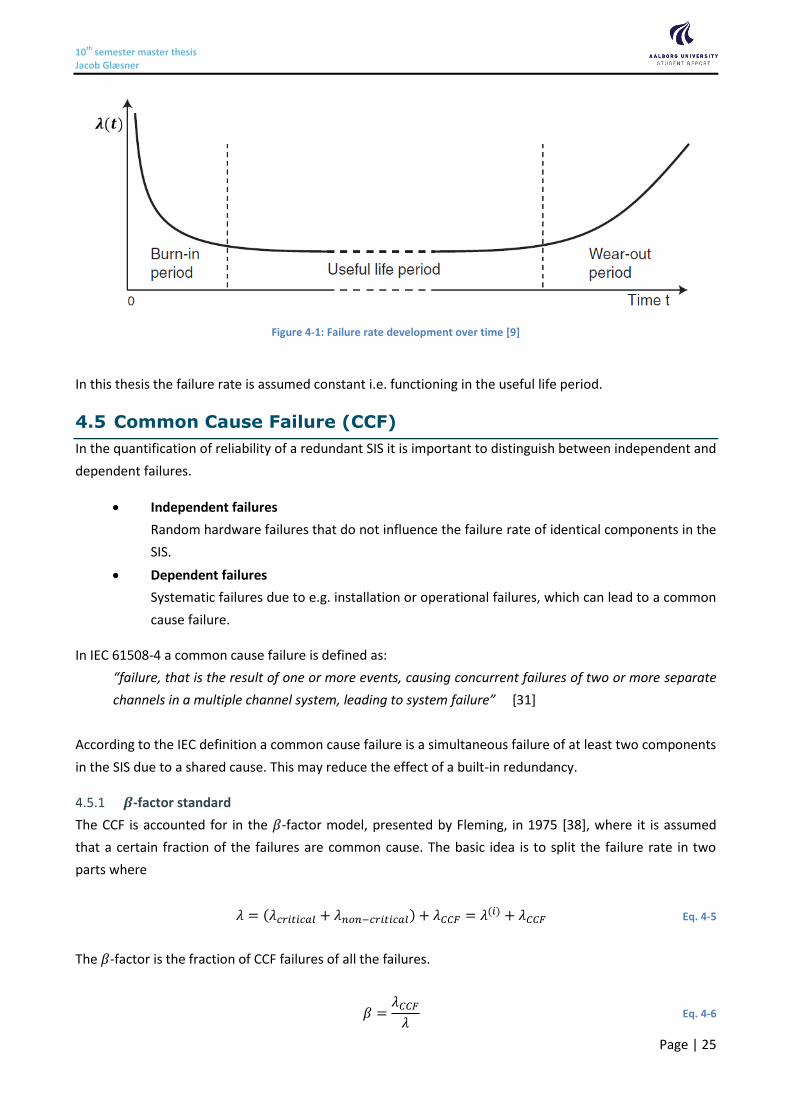
The failure rate of statistically identical and independent components follows a bathtub curve over time
with three periods as illustrated in Figure 4-1:
Burn-in period – early failures are often discovered at factory tests
Useful life period – almost constant failure rate
Wear-out period – aging equipment has an increasing failure rate
10th semester master thesis Jacob Glæsner
Page | 25
Figure 4-1: Failure rate development over time [9]
In this thesis the failure rate is assumed constant i.e. functioning in the useful life period.
4.5 Common Cause Failure (CCF)
In the quantification of reliability of a redundant SIS it is important to distinguish between independent and
dependent failures.
Independent failures
Random hardware failures that do not influence the failure rate of identical components in the
SIS.
Dependent failures
Systematic failures due to e.g. installation or operational failures, which can lead to a common
cause failure.
In IEC 61508-4 a common cause failure is defined as:
“failure, that is the result of one or more events, causing concurrent failures of two or more separate
channels in a multiple channel system, leading to system failure” [31]
According to the IEC definition a common cause failure is a simultaneous failure of at least two components
in the SIS due to a shared cause. This may reduce the effect of a built-in redundancy.
𝜷-factor standard 4.5.1
The CCF is accounted for in the 𝛽-factor model, presented by Fleming, in 1975 [38], where it is assumed
that a certain fraction of the failures are common cause. The basic idea is to split the failure rate in two
parts where
𝜆 = (𝜆𝑐𝑟𝑖𝑡𝑖𝑐𝑎𝑙 + 𝜆𝑛𝑜𝑛−𝑐𝑟𝑖𝑡𝑖𝑐𝑎𝑙) + 𝜆𝐶𝐶𝐹 = 𝜆(𝑖) + 𝜆𝐶𝐶𝐹 Eq. 4-5
The 𝛽-factor is the fraction of CCF failures of all the failures.
𝛽 =𝜆𝐶𝐶𝐹
𝜆 Eq. 4-6
10th semester master thesis Jacob Glæsner
Page | 26
and the failure rates can be expressed as
𝜆𝐶𝐶𝐹 = 𝛽𝜆 Eq. 4-7
and
𝜆(𝑖) = (1 − 𝛽)𝜆 Eq. 4-8
It is relevant to distinguish between different CCF. If 𝛽𝑈 represents the CCF rate of DU failures and 𝛽𝐷 the
DD failures, then the overall rate of dangerous CCF is:
𝜆𝐷,𝐶𝐶𝐹 = 𝛽𝑈𝜆𝐷𝑈 + 𝛽𝐷𝜆𝐷𝐷 Eq. 4-9
The weakness in the 𝛽-factor model is the lack of credit for increased redundancy due to the fact that the
individual failure rate in a high reliability SIS has almost no influence. Furthermore, the approach does not
distinguish between any moon voting. The method described in this section only applies to identical
components with constant failure rate, 𝜆𝐷𝑈 – see Section 4.5.3 page 27 for non-identical components.
𝜷-factor corrected 4.5.2
IEC 61508-6 Annex D.5 suggest an alternative method with a corrected 𝛽-factor, which is only applicable to
hardware failures. The 𝛽-factor must be calculated for each subsystem of the SIS. This is done by answering
37 questions that each give a value for calculation of a score 𝑆𝑈 or 𝑆𝐷. Each score 𝑆𝑈 or 𝑆𝐷 corresponds to a
value for the 𝛽-factor depending on the type of subsystem – see Table 4-2 .
Table 4-2: Calculation of 𝜷𝑼
or 𝜷𝑫
[4]
𝑺𝑼 or 𝑺𝑫 Corresponding value of 𝜷𝑼 or 𝜷𝑫 for the
Logic Solver Sensors or Final Elements
120 or above 0.5 % 1 %
70 to 120 1 % 2 %
45 to 70 2 % 5 %
Less than 45 5 % 10 %
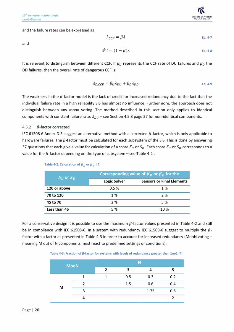
For a conservative design it is possible to use the maximum 𝛽-factor values presented in Table 4-2 and still
be in compliance with IEC 61508-6. In a system with redundancy IEC 61508-6 suggest to multiply the 𝛽-
factor with a factor as presented in Table 4-3 in order to account for increased redundancy (MooN voting –
meaning M out of N components must react to predefined settings or conditions).
Table 4-3: Fraction of β-factor for systems with levels of redundancy greater than 1oo2 [4]
MooN N
2 3 4 5
M
1 1 0.5 0.3 0.2
2 1.5 0.6 0.4
3 1.75 0.8
4 2
10th semester master thesis Jacob Glæsner
Page | 27
The numbers in Table 4-3 implies that the reduction of the 𝛽-factor is non-linear and at a certain point the
effect of increased redundancy is negligible.
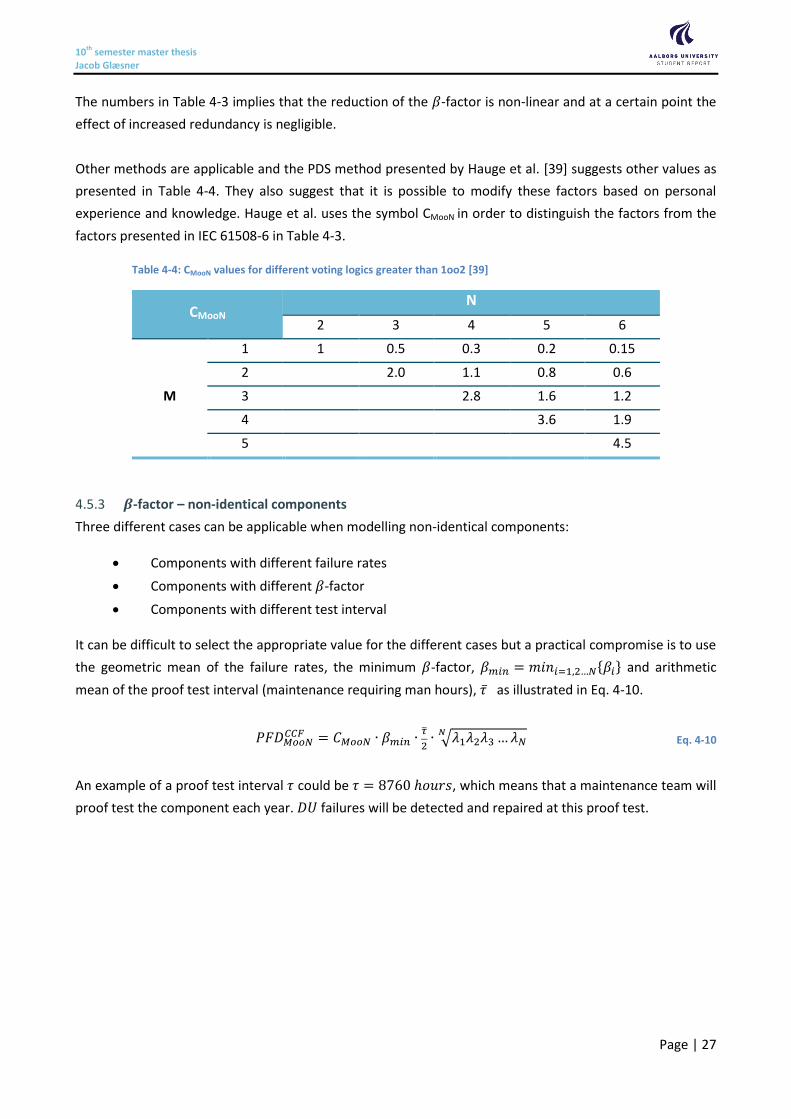
Other methods are applicable and the PDS method presented by Hauge et al. [39] suggests other values as
presented in Table 4-4. They also suggest that it is possible to modify these factors based on personal
experience and knowledge. Hauge et al. uses the symbol CMooN in order to distinguish the factors from the
factors presented in IEC 61508-6 in Table 4-3.
Table 4-4: CMooN values for different voting logics greater than 1oo2 [39]
CMooN N
2 3 4 5 6
M
1 1 0.5 0.3 0.2 0.15
2 2.0 1.1 0.8 0.6
3 2.8 1.6 1.2
4 3.6 1.9
5 4.5
𝜷-factor – non-identical components 4.5.3
Three different cases can be applicable when modelling non-identical components:
Components with different failure rates
Components with different 𝛽-factor
Components with different test interval
It can be difficult to select the appropriate value for the different cases but a practical compromise is to use
the geometric mean of the failure rates, the minimum 𝛽-factor, 𝛽𝑚𝑖𝑛 = 𝑚𝑖𝑛𝑖=1,2…𝑁{𝛽𝑖} and arithmetic
mean of the proof test interval (maintenance requiring man hours), �̅� as illustrated in Eq. 4-10.
𝑃𝐹𝐷𝑀𝑜𝑜𝑁𝐶𝐶𝐹 = 𝐶𝑀𝑜𝑜𝑁 ∙ 𝛽𝑚𝑖𝑛 ∙
�̅�
2∙ √𝜆1𝜆2𝜆3 …𝜆𝑁
𝑁 Eq. 4-10
An example of a proof test interval 𝜏 could be 𝜏 = 8760 ℎ𝑜𝑢𝑟𝑠, which means that a maintenance team will
proof test the component each year. 𝐷𝑈 failures will be detected and repaired at this proof test.
10th semester master thesis Jacob Glæsner
Page | 28
4.6 Svend HIPPS Failure Modes
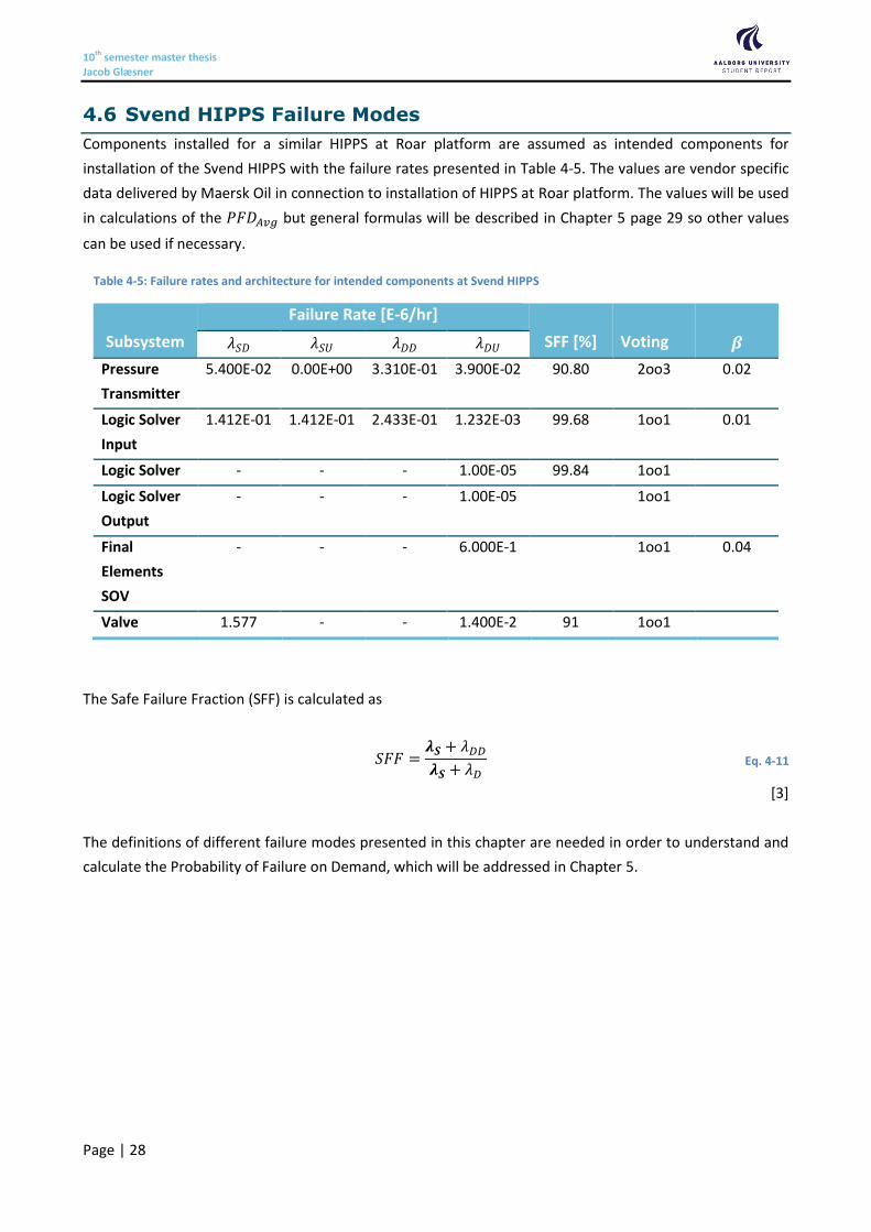
Components installed for a similar HIPPS at Roar platform are assumed as intended components for
installation of the Svend HIPPS with the failure rates presented in Table 4-5. The values are vendor specific
data delivered by Maersk Oil in connection to installation of HIPPS at Roar platform. The values will be used
in calculations of the 𝑃𝐹𝐷𝐴𝑣𝑔 but general formulas will be described in Chapter 5 page 29 so other values
can be used if necessary.
Table 4-5: Failure rates and architecture for intended components at Svend HIPPS
Subsystem
Failure Rate [E-6/hr]
SFF [%] Voting 𝜷 𝜆𝑆𝐷 𝜆𝑆𝑈 𝜆𝐷𝐷 𝜆𝐷𝑈
Pressure
Transmitter
5.400E-02 0.00E+00 3.310E-01 3.900E-02 90.80 2oo3 0.02
Logic Solver
Input
1.412E-01 1.412E-01 2.433E-01 1.232E-03 99.68 1oo1 0.01
Logic Solver - - - 1.00E-05 99.84 1oo1
Logic Solver
Output
- - - 1.00E-05 1oo1
Final
Elements
SOV
- - - 6.000E-1 1oo1 0.04
Valve 1.577 - - 1.400E-2 91 1oo1
The Safe Failure Fraction (SFF) is calculated as
𝑆𝐹𝐹 =𝝀𝑺 + 𝜆𝐷𝐷
𝝀𝑺 + 𝜆𝐷 Eq. 4-11
[3]
The definitions of different failure modes presented in this chapter are needed in order to understand and
calculate the Probability of Failure on Demand, which will be addressed in Chapter 5.
10th semester master thesis Jacob Glæsner
Page | 29
5 Probability of Failure on Demand
After introduction of Safety Instrumented Systems in Chapter 2 and different failure modes in Chapter 4 it
is relevant to continue with a description of the Probability of Failure on Demand (𝑃𝐹𝐷). The 𝑃𝐹𝐷 is used
as a quantitative value to distinguish different SIL from each other. Lower 𝑃𝐹𝐷 value results in a higher SIL
and a higher risk reduction factor (𝑅𝑅𝐹) as described in Eq. 2-1 page 14. This chapter will describe the
origin of the 𝑃𝐹𝐷 and different analytical formulas that can be used to quantify the value for relevant
architectures.
5.1 Definition of PFD
For a SIF the Probability of Failure on Demand is specified as the probability that the SIF cannot be
performed at time 𝑡 if a dangerous fault is present.
𝑃𝐹𝐷(𝑡) = Pr (𝑇ℎ𝑒 𝑆𝐼𝐹 𝑐𝑎𝑛𝑛𝑜𝑡 𝑏𝑒 𝑝𝑒𝑟𝑓𝑜𝑟𝑚𝑒𝑑 𝑎𝑡 𝑡𝑖𝑚𝑒 𝑡) Eq. 5-1
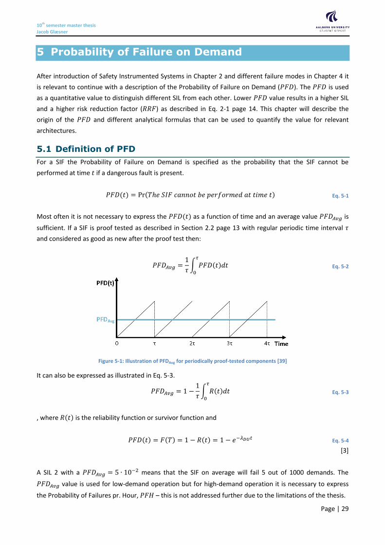
Most often it is not necessary to express the 𝑃𝐹𝐷(𝑡) as a function of time and an average value 𝑃𝐹𝐷𝐴𝑣𝑔 is
sufficient. If a SIF is proof tested as described in Section 2.2 page 13 with regular periodic time interval 𝜏
and considered as good as new after the proof test then:
𝑃𝐹𝐷𝐴𝑣𝑔 =1
𝜏∫ 𝑃𝐹𝐷(𝑡)𝑑𝑡
𝜏
0
Eq. 5-2
Figure 5-1: Illustration of PFDAvg for periodically proof-tested components [39]
It can also be expressed as illustrated in Eq. 5-3.
𝑃𝐹𝐷𝐴𝑣𝑔 = 1 −1
𝜏∫ 𝑅(𝑡)𝑑𝑡
𝜏
0
Eq. 5-3
, where 𝑅(𝑡) is the reliability function or survivor function and
𝑃𝐹𝐷(𝑡) = 𝐹(𝑇) = 1 − 𝑅(𝑡) = 1 − 𝑒−𝜆𝐷𝑈𝑡 Eq. 5-4
[3]
A SIL 2 with a 𝑃𝐹𝐷𝐴𝑣𝑔 = 5 ∙ 10−2 means that the SIF on average will fail 5 out of 1000 demands. The
𝑃𝐹𝐷𝐴𝑣𝑔 value is used for low-demand operation but for high-demand operation it is necessary to express
the Probability of Failures pr. Hour, 𝑃𝐹𝐻 – this is not addressed further due to the limitations of the thesis.
10th semester master thesis Jacob Glæsner
Page | 30
5.2 Requirements
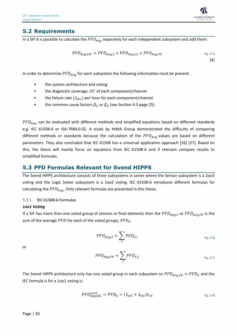
In a SIF it is possible to calculate the 𝑃𝐹𝐷𝐴𝑣𝑔 separately for each independent subsystem and add them:
𝑃𝐹𝐷𝐴𝑣𝑔,𝑆𝐼𝐹 = 𝑃𝐹𝐷𝐴𝑣𝑔,𝑆 + 𝑃𝐹𝐷𝐴𝑣𝑔,𝐿𝑆 + 𝑃𝐹𝐷𝐴𝑣𝑔,𝐹𝐸 Eq. 5-5
[4]
In order to determine 𝑃𝐹𝐷𝐴𝑣𝑔 for each subsystem the following information must be present:
• the system architecture and voting
• the diagnostic coverage, 𝐷𝐶 of each component/channel
• the failure rate (𝜆𝐷𝑈) per hour for each component/channel
• the common cause factors 𝛽𝑈 or 𝛽𝐷 (see Section 4.5 page 25)
𝑃𝐹𝐷𝐴𝑣𝑔 can be evaluated with different methods and simplified equations based on different standards
e.g. IEC 61508-6 or ISA-TR84.0.02. A study by HIMA Group demonstrated the difficulty of comparing
different methods or standards because the calculation of the 𝑃𝐹𝐷𝐴𝑣𝑔-values are based on different
parameters. They also concluded that IEC 61508 has a universal application approach [26] [27]. Based on
this, the thesis will mainly focus on equations from IEC 61508-6 and if relevant compare results to
simplified formulas.
5.3 PFD Formulas Relevant for Svend HIPPS
The Svend HIPPS architecture consists of three subsystems in series where the Sensor subsystem is a 2oo3
voting and the Logic Solver subsystem is a 1oo2 voting. IEC 61508-6 introduces different formulas for
calculating the 𝑃𝐹𝐷𝐴𝑣𝑔. Only relevant formulas are presented in this thesis.
IEC 61508-6 Formulas 5.3.1
1oo1 Voting
If a SIF has more than one voted group of sensors or final elements then the 𝑃𝐹𝐷𝐴𝑣𝑔,𝑆 or 𝑃𝐹𝐷𝐴𝑣𝑔,𝐹𝐸 is the
sum of the average 𝑃𝐹𝐷 for each of the voted groups, 𝑃𝐹𝐷𝐺.
𝑃𝐹𝐷𝐴𝑣𝑔,𝑆 = ∑𝑃𝐹𝐷𝐺,𝑖
𝑖
Eq. 5-6
or
𝑃𝐹𝐷𝐴𝑣𝑔,𝐹𝐸 = ∑𝑃𝐹𝐷𝐺,𝑗
𝑗
Eq. 5-7
The Svend HIPPS architecture only has one voted group in each subsystem so 𝑃𝐹𝐷𝐴𝑣𝑔,𝐹𝐸 = 𝑃𝐹𝐷𝐺 and the
IEC formula is for a 1oo1 voting is:
𝑃𝐹𝐷𝐴𝑣𝑔,𝐼𝐸𝐶1𝑜𝑜1 = 𝑃𝐹𝐷𝐺 = (𝜆𝐷𝐷 + 𝜆𝐷𝑈)𝑡𝐶𝐸 Eq. 5-8
10th semester master thesis Jacob Glæsner
Page | 31
where 𝑡𝐶𝐸 is the combined down time in hours for all components in the subsystem.
𝑡𝐶𝐸 =𝜆𝐷𝑈
𝜆𝐷(𝜏
2+ 𝑀𝑅𝑇) +
𝜆𝐷𝐷
𝜆𝐷𝑀𝑇𝑇𝑅 Eq. 5-9
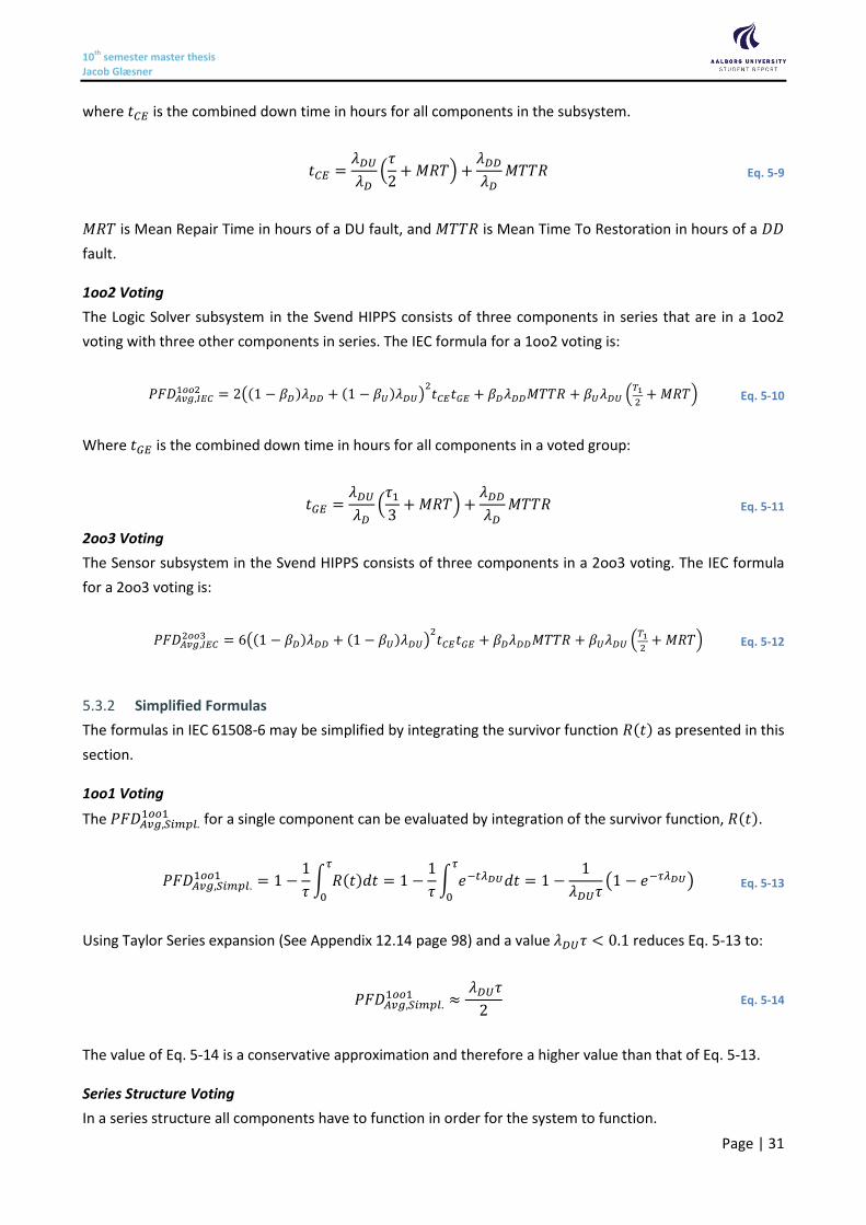
𝑀𝑅𝑇 is Mean Repair Time in hours of a DU fault, and 𝑀𝑇𝑇𝑅 is Mean Time To Restoration in hours of a 𝐷𝐷
fault.
1oo2 Voting
The Logic Solver subsystem in the Svend HIPPS consists of three components in series that are in a 1oo2
voting with three other components in series. The IEC formula for a 1oo2 voting is:
𝑃𝐹𝐷𝐴𝑣𝑔,𝐼𝐸𝐶1𝑜𝑜2 = 2((1 − 𝛽𝐷)𝜆𝐷𝐷 + (1 − 𝛽𝑈)𝜆𝐷𝑈)
2𝑡𝐶𝐸𝑡𝐺𝐸 + 𝛽𝐷𝜆𝐷𝐷𝑀𝑇𝑇𝑅 + 𝛽𝑈𝜆𝐷𝑈 (
𝑇1
2+ 𝑀𝑅𝑇) Eq. 5-10
Where 𝑡𝐺𝐸 is the combined down time in hours for all components in a voted group:
𝑡𝐺𝐸 =𝜆𝐷𝑈
𝜆𝐷(𝜏1
3+ 𝑀𝑅𝑇) +
𝜆𝐷𝐷
𝜆𝐷𝑀𝑇𝑇𝑅 Eq. 5-11
2oo3 Voting
The Sensor subsystem in the Svend HIPPS consists of three components in a 2oo3 voting. The IEC formula
for a 2oo3 voting is:
𝑃𝐹𝐷𝐴𝑣𝑔,𝐼𝐸𝐶2𝑜𝑜3 = 6((1 − 𝛽𝐷)𝜆𝐷𝐷 + (1 − 𝛽𝑈)𝜆𝐷𝑈)
2𝑡𝐶𝐸𝑡𝐺𝐸 + 𝛽𝐷𝜆𝐷𝐷𝑀𝑇𝑇𝑅 + 𝛽𝑈𝜆𝐷𝑈 (
𝑇1
2+ 𝑀𝑅𝑇) Eq. 5-12
Simplified Formulas 5.3.2
The formulas in IEC 61508-6 may be simplified by integrating the survivor function 𝑅(𝑡) as presented in this
section.
1oo1 Voting
The 𝑃𝐹𝐷𝐴𝑣𝑔,𝑆𝑖𝑚𝑝𝑙.1𝑜𝑜1 for a single component can be evaluated by integration of the survivor function, 𝑅(𝑡).
𝑃𝐹𝐷𝐴𝑣𝑔,𝑆𝑖𝑚𝑝𝑙.1𝑜𝑜1 = 1 −
1
𝜏∫ 𝑅(𝑡)𝑑𝑡
𝜏
0
= 1 −1
𝜏∫ 𝑒−𝑡𝜆𝐷𝑈𝑑𝑡
𝜏
0
= 1 −1
𝜆𝐷𝑈𝜏(1 − 𝑒−𝜏𝜆𝐷𝑈) Eq. 5-13
Using Taylor Series expansion (See Appendix 12.14 page 98) and a value 𝜆𝐷𝑈𝜏 < 0.1 reduces Eq. 5-13 to:
𝑃𝐹𝐷𝐴𝑣𝑔,𝑆𝑖𝑚𝑝𝑙.1𝑜𝑜1 ≈
𝜆𝐷𝑈𝜏
2 Eq. 5-14
The value of Eq. 5-14 is a conservative approximation and therefore a higher value than that of Eq. 5-13.
Series Structure Voting
In a series structure all components have to function in order for the system to function.
10th semester master thesis Jacob Glæsner
Page | 32
The survivor function is:
𝑅(𝑡) = 𝑒−(∑ 𝜆𝐷𝑈,𝑖𝑛𝑖 )𝑡 Eq. 5-15
With integration, Taylor Series expansion, reduction and 𝜆𝐷𝑈,𝑖𝜏 < 0.1 for all 𝑖, then
𝑃𝐹𝐷𝐴𝑣𝑔,𝑆𝑖𝑚𝑝𝑙.𝑛𝑜𝑜𝑛 ≈ ∑𝑃𝐹𝐷𝐴𝑣𝑔,𝑖
𝑛
𝑖=1
Eq. 5-16
1oo2 Voting
The Logic Solver components are placed in two series structures that are in a 1oo2 voting. The survivor
function is
𝑅(𝑡) = 𝑒−𝑡𝜆𝐷𝑈,1 + 𝑒−𝑡𝜆𝐷𝑈,2 − 𝑒−𝑡(𝜆𝐷𝑈,1+𝜆𝐷𝑈,2) Eq. 5-17
With integration, Taylor Series expansion, and reduction [3]:
𝑃𝐹𝐷𝐴𝑣𝑔,𝑆𝑖𝑚𝑝𝑙.1𝑜𝑜2 ≈
𝜆𝐷𝑈,1𝜆𝐷𝑈,2𝜏2
3 Eq. 5-18
And for identical components
𝑃𝐹𝐷𝐴𝑣𝑔,𝑆𝑖𝑚𝑝𝑙.1𝑜𝑜2 ≈
(𝜏𝜆𝐷𝑈)2
3 Eq. 5-19
Furthermore the 𝑃𝐹𝐷𝐶𝐶𝐹 must be added – see Eq. 5-22.
2oo3 Voting
It can be time consuming to integrate a survivor function of a 2oo3 architecture so a simplified approach
may be used. The 2oo3 voting can be replaced by a series structure of 1oo2, so
𝑃𝐹𝐷𝐴𝑣𝑔,𝑆𝑖𝑚𝑝𝑙.2𝑜𝑜3 ≈
𝜆𝐷𝑈,1𝜆𝐷𝑈,2𝜏2
3+
𝜆𝐷𝑈,1𝜆𝐷𝑈,3𝜏2
3+
𝜆𝐷𝑈,2𝜆𝐷𝑈,3𝜏2
3 Eq. 5-20
=(𝜆𝐷𝑈,1𝜆𝐷𝑈,2 + 𝜆𝐷𝑈,1𝜆𝐷𝑈,3 + 𝜆𝐷𝑈,2𝜆𝐷𝑈,3)𝜏
2
3
[3]
And for identical components:
𝑃𝐹𝐷𝐴𝑣𝑔,𝑆𝑖𝑚𝑝𝑙.2𝑜𝑜3 ≈
3(𝜏𝜆𝐷𝑈)2
3= 3𝑃𝐹𝐷𝐴𝑣𝑔
1𝑜𝑜2 Eq. 5-21
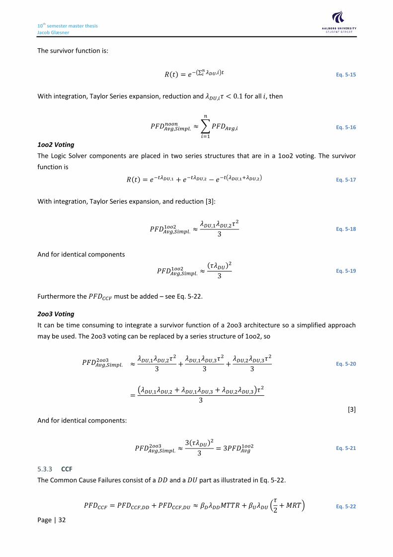
CCF 5.3.3
The Common Cause Failures consist of a 𝐷𝐷 and a 𝐷𝑈 part as illustrated in Eq. 5-22.
𝑃𝐹𝐷𝐶𝐶𝐹 = 𝑃𝐹𝐷𝐶𝐶𝐹,𝐷𝐷 + 𝑃𝐹𝐷𝐶𝐶𝐹,𝐷𝑈 ≈ 𝛽𝐷𝜆𝐷𝐷𝑀𝑇𝑇𝑅 + 𝛽𝑈𝜆𝐷𝑈 (𝜏
2+ 𝑀𝑅𝑇) Eq. 5-22
10th semester master thesis Jacob Glæsner
Page | 33
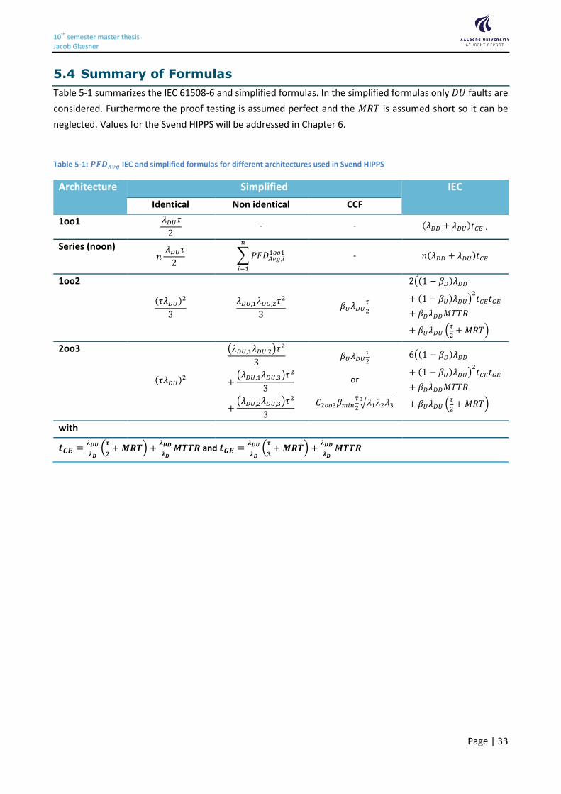
5.4 Summary of Formulas
Table 5-1 summarizes the IEC 61508-6 and simplified formulas. In the simplified formulas only 𝐷𝑈 faults are
considered. Furthermore the proof testing is assumed perfect and the 𝑀𝑅𝑇 is assumed short so it can be
neglected. Values for the Svend HIPPS will be addressed in Chapter 6.
Table 5-1: 𝑷𝑭𝑫𝑨𝒗𝒈 IEC and simplified formulas for different architectures used in Svend HIPPS
Architecture Simplified IEC
Identical Non identical CCF
1oo1 𝜆𝐷𝑈𝜏
2 - - (𝜆𝐷𝐷 + 𝜆𝐷𝑈)𝑡𝐶𝐸 ,
Series (noon) 𝑛
𝜆𝐷𝑈𝜏
2 ∑𝑃𝐹𝐷𝐴𝑣𝑔,𝑖
1𝑜𝑜1
𝑛
𝑖=1
- 𝑛(𝜆𝐷𝐷 + 𝜆𝐷𝑈)𝑡𝐶𝐸
1oo2
(𝜏𝜆𝐷𝑈)2
3
𝜆𝐷𝑈,1𝜆𝐷𝑈,2𝜏2
3 𝛽𝑈𝜆𝐷𝑈
𝜏
2
2((1 − 𝛽𝐷)𝜆𝐷𝐷
+ (1 − 𝛽𝑈)𝜆𝐷𝑈)2𝑡𝐶𝐸𝑡𝐺𝐸
+ 𝛽𝐷𝜆𝐷𝐷𝑀𝑇𝑇𝑅
+ 𝛽𝑈𝜆𝐷𝑈 (𝜏
2+ 𝑀𝑅𝑇)
2oo3
(𝜏𝜆𝐷𝑈)2
(𝜆𝐷𝑈,1𝜆𝐷𝑈,2)𝜏2
3
+(𝜆𝐷𝑈,1𝜆𝐷𝑈,3)𝜏
2
3
+(𝜆𝐷𝑈,2𝜆𝐷𝑈,3)𝜏
2
3
𝛽𝑈𝜆𝐷𝑈𝜏
2
or
𝐶2𝑜𝑜3𝛽𝑚𝑖𝑛�̅�
2√𝜆1𝜆2𝜆33
6((1 − 𝛽𝐷)𝜆𝐷𝐷
+ (1 − 𝛽𝑈)𝜆𝐷𝑈)2𝑡𝐶𝐸𝑡𝐺𝐸
+ 𝛽𝐷𝜆𝐷𝐷𝑀𝑇𝑇𝑅
+ 𝛽𝑈𝜆𝐷𝑈 (𝜏
2+ 𝑀𝑅𝑇)
with
𝒕𝑪𝑬 =𝝀𝑫𝑼
𝝀𝑫(
𝝉
𝟐+ 𝑴𝑹𝑻) +
𝝀𝑫𝑫
𝝀𝑫𝑴𝑻𝑻𝑹 and 𝒕𝑮𝑬 =
𝝀𝑫𝑼
𝝀𝑫(
𝝉
𝟑+ 𝑴𝑹𝑻) +
𝝀𝑫𝑫
𝝀𝑫𝑴𝑻𝑻𝑹
10th semester master thesis Jacob Glæsner
Page | 34
6 Reliability Block Diagrams
As described in Figure 1-2 page 5 Reliability Block Diagrams (RBD) is one of the quantitative methods to
evaluate the reliability of a SIS. This chapter will describe how RBD is used to determine the reliability of the
Svend HIPPS.
A Reliability Block Diagram (RBD) shows the successful functioning of a system. It is important to emphasize
that the pictorial representation of the individual components merely shows the functioning. This is not
necessarily equivalent to the physical order of the components. The RBD can be used to represent logical
equations of Boolean variables. RBD can be used for qualitative and quantitative analysis of a system.
6.1 Assumptions and Definitions
The RBD is used to model the functioning of the system based on some fundamental assumptions and
definitions of states as described in this section 6.1. These assumptions have to be fulfilled in order to use
analytical calculations presented in IEC 61078 [40]. Otherwise Monte Carlo simulations can be used but this
master thesis has been limited to analytical calculations as described in Section 1.3 page 4.
State of system 6.1.1
The state of the whole system can be described by the structure function
𝜙(𝑿) = 𝜙(𝑥1, 𝑥2, 𝑥3, …… , 𝑥𝑛) Eq. 6-1
𝜙(𝑿) = {1 𝑖𝑓 𝑠𝑦𝑠𝑡𝑒𝑚 𝑖𝑠 𝑓𝑢𝑛𝑐𝑡𝑖𝑜𝑛𝑖𝑛𝑔0 𝑜𝑡ℎ𝑒𝑟𝑤𝑖𝑐𝑒
} Eq. 6-2
The system has only two states:
Functioning (“up” state)
Failed (“down” state)
The RBD links the logic between the up state of the system and the up state of the individual components.
State of components 6.1.2
Each component in a system is modelled by independent working blocks in the RBD. Each component can
have only two possible states:
Functioning (“up” state)
Failed (“down” state)
If the state 𝑖 is represented by a state variable, then
𝑥𝑖 = {1 𝑖𝑓 𝑐𝑜𝑚𝑝𝑜𝑛𝑒𝑛𝑡 𝑖 𝑖𝑠 𝑓𝑢𝑛𝑐𝑡𝑖𝑜𝑛𝑖𝑛𝑔0 𝑜𝑡ℎ𝑒𝑟𝑤𝑖𝑐𝑒
} Eq. 6-3
The state vector is
𝑿 = (𝑥1, 𝑥2, 𝑥3, …… , 𝑥𝑛) Eq. 6-4

10th semester master thesis Jacob Glæsner
Page | 35
6.2 Graphical & Mathematical Illustration of Boolean Logic [40]
With the defined state of the system and components the graphical RBD can be constructed and represent
a Boolean logic and mathematical expression of the system structure. Different building blocks and Boolean
logic operators for illustration of the system structure are presented in Figure 6-1.
Static RBD •,∩ AND logic
Dynamic RBD +,∪ OR logic
Figure 6-1: RBD type and Boolean logic operators
Series structures 6.2.1
In a series structure, as illustrated in Figure 6-2, all components need to function in order for the system to
function.
Figure 6-2: Series RBD
The series RBD represents the Boolean logic in Eq. 6-5 and mathematical expression in Eq. 6-6.
ϕ(𝑿) = 𝑥1 • 𝑥2 • 𝑥3 • … • 𝑥𝑛 = 𝑥1 ∩ 𝑥2 ∩ 𝑥3 ∩ …∩ 𝑥𝑛 Eq. 6-5
ϕ(𝑿) = 𝑥1𝑥2𝑥3 ∙ … ∙ 𝑥𝑛 = ∏𝑥𝑖
𝑛
𝑖=1
Eq. 6-6
Parallel structures and m out of n (moon) structures 6.2.2
In a parallel structure, illustrated in Figure 6-3, only one component in up state is required for the system to
be in up state. This structure is used when redundant components are implemented in the system.
Figure 6-3: Parallel RBD
Figure 6-4: moon RBD

10th semester master thesis Jacob Glæsner
Page | 36
The parallel RBD represents the Boolean logic in Eq. 6-7 and mathematical expression in Eq. 6-8.
ϕ(𝑿) = 𝑥1 + 𝑥2 + 𝑥3 + ⋯+ 𝑥𝑛 = 𝑥1 ∪ 𝑥2 ∪ 𝑥3 ∪ …∪ 𝑥𝑛 Eq. 6-7
ϕ(𝑿) = 1 − (1 − 𝑥1)(1 − 𝑥2)(1 − 𝑥3) ∙∙∙ (1 − 𝑥𝑛) = 1 − ∏(1 − 𝑥𝑖)
𝑛
𝑖=1
Eq. 6-8
A special case of a parallel RBD is when a voting is implemented in the logic and 𝑚 out of 𝑛 components are
required to be in up state in order for the system to be in up state. The RBD of this case is illustrated in
Figure 6-4 and also illustrated with an example of a 2oo3 voting in Figure 6-5 and Figure 6-6.
Figure 6-5: 2oo3 RBD
Figure 6-6: Equivalent 2oo3 RBD
The 2oo3 RBD represents the Boolean logic in Eq. 6-9 and mathematical expression in Eq. 6-10.
ϕ(𝑿) = 𝑥1 • 𝑥2 + 𝑥1 • 𝑥3 + 𝑥2 • 𝑥3 = 𝑥1 ∩ 𝑥2 ∪ 𝑥1 ∩ 𝑥3 ∪ 𝑥2 ∩ 𝑥3 Eq. 6-9
ϕ(𝑿) = 𝑥1𝑥2 + 𝑥1𝑥3 + 𝑥2𝑥3 − 2𝑥1𝑥2𝑥3 Eq. 6-10
See Appendix 12.12 page 93 for derivation of Eq. 6-10.
Other structures 6.2.3
A complex system can be represented by a mix of subsystems of series, parallel, and moon structures. In
large and complex systems it is possible to use transfer gates and it is also possible for systems to share
blocks.
6.3 Probability Calculations
The state variable 𝑥𝑖 defined in Section 6.1 page 34 is deterministic as it can be in either up state or down
state. In reliability analysis the state variable is random and dependent on time, which is illustrated with the
variable, 𝑋𝑖(𝑡). With a random variable it is possible to determine the probability, 𝑃𝑟, of a component, 𝑖, or
system, 𝑠, to be in either up state Pr(𝑋𝑖/𝑠(𝑡) = 1) or down state Pr(𝑋𝑖/𝑠(𝑡) = 0).
Pr(𝑋𝑖/𝑠(𝑡) = 1) = 𝑃𝑟(𝑇 > 𝑡) = 𝑝𝑖/𝑠(𝑡) Eq. 6-11
Pr(𝑋𝑖/𝑠(𝑡) = 0) = 𝑃𝑟(𝑇 < 𝑡) = 1 − 𝑝𝑖/𝑠(𝑡) Eq. 6-12
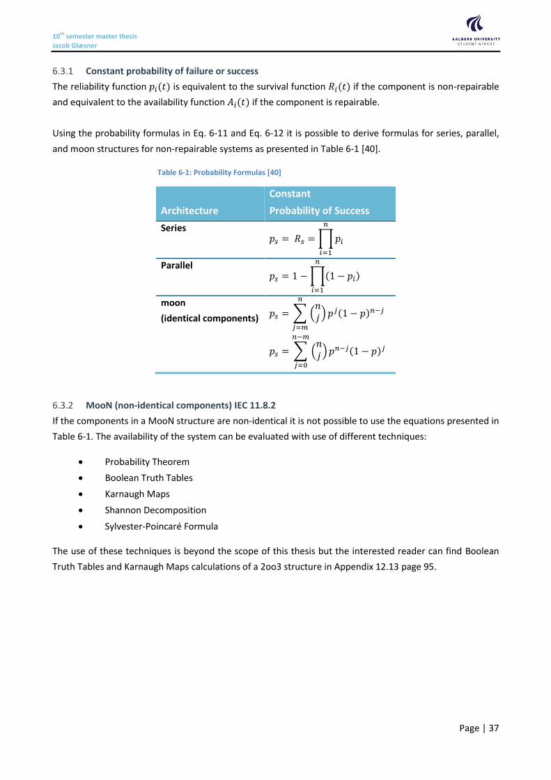
10th semester master thesis Jacob Glæsner
Page | 37
Constant probability of failure or success 6.3.1
The reliability function 𝑝𝑖(𝑡) is equivalent to the survival function 𝑅𝑖(𝑡) if the component is non-repairable
and equivalent to the availability function 𝐴𝑖(𝑡) if the component is repairable.
Using the probability formulas in Eq. 6-11 and Eq. 6-12 it is possible to derive formulas for series, parallel,
and moon structures for non-repairable systems as presented in Table 6-1 [40].
Table 6-1: Probability Formulas [40]
Architecture
Constant
Probability of Success
Series 𝑝𝑠 = 𝑅𝑠 = ∏𝑝𝑖
𝑛
𝑖=1
Parallel 𝑝𝑠 = 1 − ∏(1 − 𝑝𝑖)
𝑛
𝑖=1
moon
(identical components) 𝑝𝑠 = ∑ (𝑛𝑗)
𝑛
𝑗=𝑚
𝑝𝑗(1 − 𝑝)𝑛−𝑗
𝑝𝑠 = ∑ (𝑛𝑗)
𝑛−𝑚
𝑗=0
𝑝𝑛−𝑗(1 − 𝑝)𝑗
MooN (non-identical components) IEC 11.8.2 6.3.2
If the components in a MooN structure are non-identical it is not possible to use the equations presented in
Table 6-1. The availability of the system can be evaluated with use of different techniques:
Probability Theorem
Boolean Truth Tables
Karnaugh Maps
Shannon Decomposition
Sylvester-Poincaré Formula
The use of these techniques is beyond the scope of this thesis but the interested reader can find Boolean
Truth Tables and Karnaugh Maps calculations of a 2oo3 structure in Appendix 12.13 page 95.
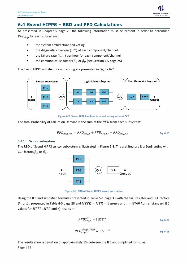
10th semester master thesis Jacob Glæsner
Page | 38
6.4 Svend HIPPS – RBD and PFD Calculations
As presented in Chapter 5 page 29 the following information must be present in order to determine
𝑃𝐹𝐷𝐴𝑣𝑔 for each subsystem:
• the system architecture and voting
• the diagnostic coverage (𝐷𝐶) of each component/channel
• the failure rate (𝜆𝐷𝑈) per hour for each component/channel
• the common cause factors 𝛽𝑈 or 𝛽𝐷 (see Section 4.5 page 25)
The Svend HIPPS architecture and voting are presented in Figure 6-7.
Figure 6-7: Svend HIPPS architecture and voting without CCF
The total Probability of Failure on Demand is the sum of the 𝑃𝐹𝐷 from each subsystem:
𝑃𝐹𝐷𝐴𝑣𝑔,𝑆𝐼𝐹 = 𝑃𝐹𝐷𝐴𝑣𝑔,𝑆 + 𝑃𝐹𝐷𝐴𝑣𝑔,𝐿𝑆 + 𝑃𝐹𝐷𝐴𝑣𝑔,𝐹𝐸 Eq. 6-13
Sensor subsystem 6.4.1
The RBD of Svend HIPPS sensor subsystem is illustrated in Figure 6-8. The architecture is a 2oo3 voting with
CCF factors 𝛽𝑈 or 𝛽𝐷.
Figure 6-8: RBD of Svend HIPPS sensor subsystem
Using the IEC and simplified formulas presented in Table 5-1 page 33 with the failure rates and CCF factors
𝛽𝑈 or 𝛽𝐷 presented in Table 4-5 page 28 and 𝑀𝑇𝑇𝑅 = 𝑀𝑇𝑅 = 8 ℎ𝑜𝑢𝑟𝑠 and 𝜏 = 8760 ℎ𝑜𝑢𝑟𝑠 (standard IEC
values for 𝑀𝑇𝑇𝑅, 𝑀𝑇𝑅 and 𝜏) results in
𝑃𝐹𝐷𝐴𝑣𝑔,𝑆𝐼𝐸𝐶 = 3.57𝐸−6 Eq. 6-14
𝑃𝐹𝐷𝐴𝑣𝑔,𝑆𝑆𝑖𝑚𝑝𝑙𝑖𝑓𝑖𝑒𝑑
= 3.53𝐸−6 Eq. 6-15
The results show a deviation of approximately 1% between the IEC and simplified formulas.
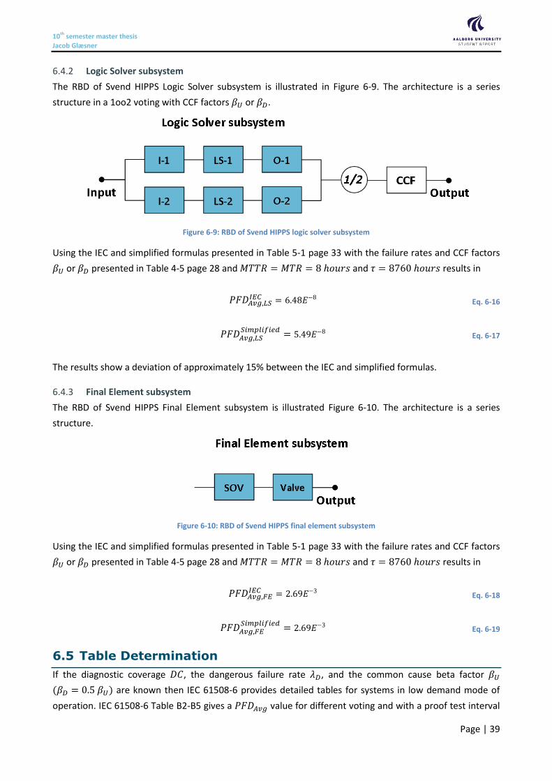
10th semester master thesis Jacob Glæsner
Page | 39
Logic Solver subsystem 6.4.2
The RBD of Svend HIPPS Logic Solver subsystem is illustrated in Figure 6-9. The architecture is a series
structure in a 1oo2 voting with CCF factors 𝛽𝑈 or 𝛽𝐷.
Figure 6-9: RBD of Svend HIPPS logic solver subsystem
Using the IEC and simplified formulas presented in Table 5-1 page 33 with the failure rates and CCF factors
𝛽𝑈 or 𝛽𝐷 presented in Table 4-5 page 28 and 𝑀𝑇𝑇𝑅 = 𝑀𝑇𝑅 = 8 ℎ𝑜𝑢𝑟𝑠 and 𝜏 = 8760 ℎ𝑜𝑢𝑟𝑠 results in
𝑃𝐹𝐷𝐴𝑣𝑔,𝐿𝑆𝐼𝐸𝐶 = 6.48𝐸−8 Eq. 6-16
𝑃𝐹𝐷𝐴𝑣𝑔,𝐿𝑆𝑆𝑖𝑚𝑝𝑙𝑖𝑓𝑖𝑒𝑑
= 5.49𝐸−8 Eq. 6-17
The results show a deviation of approximately 15% between the IEC and simplified formulas.
Final Element subsystem 6.4.3
The RBD of Svend HIPPS Final Element subsystem is illustrated Figure 6-10. The architecture is a series
structure.
Figure 6-10: RBD of Svend HIPPS final element subsystem
Using the IEC and simplified formulas presented in Table 5-1 page 33 with the failure rates and CCF factors
𝛽𝑈 or 𝛽𝐷 presented in Table 4-5 page 28 and 𝑀𝑇𝑇𝑅 = 𝑀𝑇𝑅 = 8 ℎ𝑜𝑢𝑟𝑠 and 𝜏 = 8760 ℎ𝑜𝑢𝑟𝑠 results in
𝑃𝐹𝐷𝐴𝑣𝑔,𝐹𝐸𝐼𝐸𝐶 = 2.69𝐸−3 Eq. 6-18
𝑃𝐹𝐷𝐴𝑣𝑔,𝐹𝐸𝑆𝑖𝑚𝑝𝑙𝑖𝑓𝑖𝑒𝑑
= 2.69𝐸−3 Eq. 6-19
6.5 Table Determination
If the diagnostic coverage 𝐷𝐶, the dangerous failure rate 𝜆𝐷, and the common cause beta factor 𝛽𝑈
(𝛽𝐷 = 0.5 𝛽𝑈) are known then IEC 61508-6 provides detailed tables for systems in low demand mode of
operation. IEC 61508-6 Table B2-B5 gives a 𝑃𝐹𝐷𝐴𝑣𝑔 value for different voting and with a proof test interval
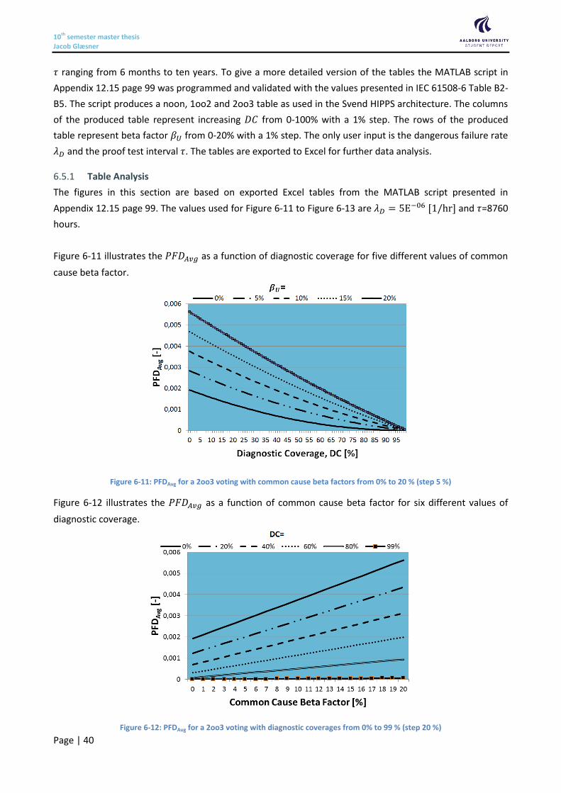
10th semester master thesis Jacob Glæsner
Page | 40
𝜏 ranging from 6 months to ten years. To give a more detailed version of the tables the MATLAB script in
Appendix 12.15 page 99 was programmed and validated with the values presented in IEC 61508-6 Table B2-
B5. The script produces a noon, 1oo2 and 2oo3 table as used in the Svend HIPPS architecture. The columns
of the produced table represent increasing 𝐷𝐶 from 0-100% with a 1% step. The rows of the produced
table represent beta factor 𝛽𝑈 from 0-20% with a 1% step. The only user input is the dangerous failure rate
𝜆𝐷 and the proof test interval 𝜏. The tables are exported to Excel for further data analysis.
Table Analysis 6.5.1
The figures in this section are based on exported Excel tables from the MATLAB script presented in
Appendix 12.15 page 99. The values used for Figure 6-11 to Figure 6-13 are 𝜆𝐷 = 5E−06 [1/hr] and 𝜏=8760
hours.
Figure 6-11 illustrates the 𝑃𝐹𝐷𝐴𝑣𝑔 as a function of diagnostic coverage for five different values of common
cause beta factor.
Figure 6-11: PFDAvg for a 2oo3 voting with common cause beta factors from 0% to 20 % (step 5 %)
Figure 6-12 illustrates the 𝑃𝐹𝐷𝐴𝑣𝑔 as a function of common cause beta factor for six different values of
diagnostic coverage.
Figure 6-12: PFDAvg for a 2oo3 voting with diagnostic coverages from 0% to 99 % (step 20 %)
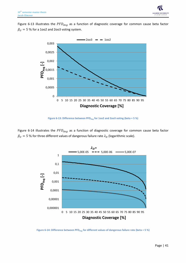
10th semester master thesis Jacob Glæsner
Page | 41
Figure 6-13 illustrates the 𝑃𝐹𝐷𝐴𝑣𝑔 as a function of diagnostic coverage for common cause beta factor
𝛽𝑈 = 5 % for a 1oo2 and 2oo3 voting system.
Figure 6-13: Difference between PFDAvg for 1oo2 and 2oo3 voting (beta = 5 %)
Figure 6-14 illustrates the 𝑃𝐹𝐷𝐴𝑣𝑔 as a function of diagnostic coverage for common cause beta factor
𝛽𝑈 = 5 % for three different values of dangerous failure rate 𝜆𝐷 (logarithmic scale).
Figure 6-14: Difference between PFDAvg for different values of dangerous failure rate (beta = 5 %)
0
0,0005
0,001
0,0015
0,002
0,0025
0,003
0 5 10 15 20 25 30 35 40 45 50 55 60 65 70 75 80 85 90 95
PFD
Avg
[-]
Diagnostic Coverage [%]
2oo3 1oo2
0,000001
0,00001
0,0001
0,001
0,01
0,1
1
0 5 10 15 20 25 30 35 40 45 50 55 60 65 70 75 80 85 90 95
PFD
Avg
[-]
Diagnostic Coverage [%]
5,00E-05 5,00E-06 5,00E-07
𝝀𝑫=
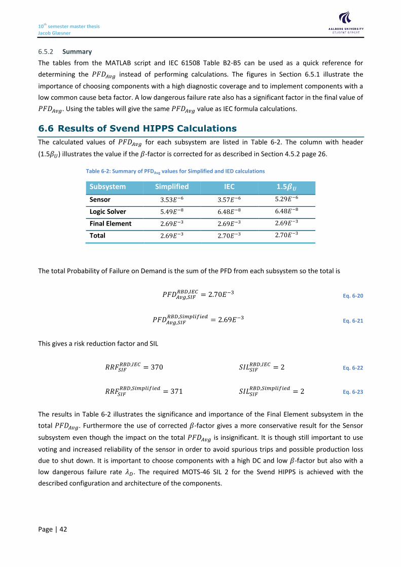
10th semester master thesis Jacob Glæsner
Page | 42
Summary 6.5.2
The tables from the MATLAB script and IEC 61508 Table B2-B5 can be used as a quick reference for
determining the 𝑃𝐹𝐷𝐴𝑣𝑔 instead of performing calculations. The figures in Section 6.5.1 illustrate the
importance of choosing components with a high diagnostic coverage and to implement components with a
low common cause beta factor. A low dangerous failure rate also has a significant factor in the final value of
𝑃𝐹𝐷𝐴𝑣𝑔. Using the tables will give the same 𝑃𝐹𝐷𝐴𝑣𝑔 value as IEC formula calculations.
6.6 Results of Svend HIPPS Calculations
The calculated values of 𝑃𝐹𝐷𝐴𝑣𝑔 for each subsystem are listed in Table 6-2. The column with header
(1.5𝛽𝑈) illustrates the value if the 𝛽-factor is corrected for as described in Section 4.5.2 page 26.
Table 6-2: Summary of PFDAvg values for Simplified and IED calculations
Subsystem Simplified IEC 1.5𝜷𝑼
Sensor 3.53𝐸−6 3.57𝐸−6 5.29𝐸−6
Logic Solver 5.49𝐸−8 6.48𝐸−8 6.48𝐸−8
Final Element 2.69𝐸−3 2.69𝐸−3 2.69𝐸−3
Total 2.69𝐸−3 2.70𝐸−3 2.70𝐸−3
The total Probability of Failure on Demand is the sum of the PFD from each subsystem so the total is
𝑃𝐹𝐷𝐴𝑣𝑔,𝑆𝐼𝐹𝑅𝐵𝐷,𝐼𝐸𝐶 = 2.70𝐸−3 Eq. 6-20
𝑃𝐹𝐷𝐴𝑣𝑔,𝑆𝐼𝐹𝑅𝐵𝐷,𝑆𝑖𝑚𝑝𝑙𝑖𝑓𝑖𝑒𝑑
= 2.69𝐸−3 Eq. 6-21
This gives a risk reduction factor and SIL
𝑅𝑅𝐹𝑆𝐼𝐹𝑅𝐵𝐷,𝐼𝐸𝐶 = 370 𝑆𝐼𝐿𝑆𝐼𝐹
𝑅𝐵𝐷,𝐼𝐸𝐶 = 2 Eq. 6-22
𝑅𝑅𝐹𝑆𝐼𝐹𝑅𝐵𝐷,𝑆𝑖𝑚𝑝𝑙𝑖𝑓𝑖𝑒𝑑
= 371 𝑆𝐼𝐿𝑆𝐼𝐹𝑅𝐵𝐷,𝑆𝑖𝑚𝑝𝑙𝑖𝑓𝑖𝑒𝑑
= 2 Eq. 6-23
The results in Table 6-2 illustrates the significance and importance of the Final Element subsystem in the
total 𝑃𝐹𝐷𝐴𝑣𝑔. Furthermore the use of corrected 𝛽-factor gives a more conservative result for the Sensor
subsystem even though the impact on the total 𝑃𝐹𝐷𝐴𝑣𝑔 is insignificant. It is though still important to use
voting and increased reliability of the sensor in order to avoid spurious trips and possible production loss
due to shut down. It is important to choose components with a high DC and low 𝛽-factor but also with a
low dangerous failure rate 𝜆𝐷. The required MOTS-46 SIL 2 for the Svend HIPPS is achieved with the
described configuration and architecture of the components.
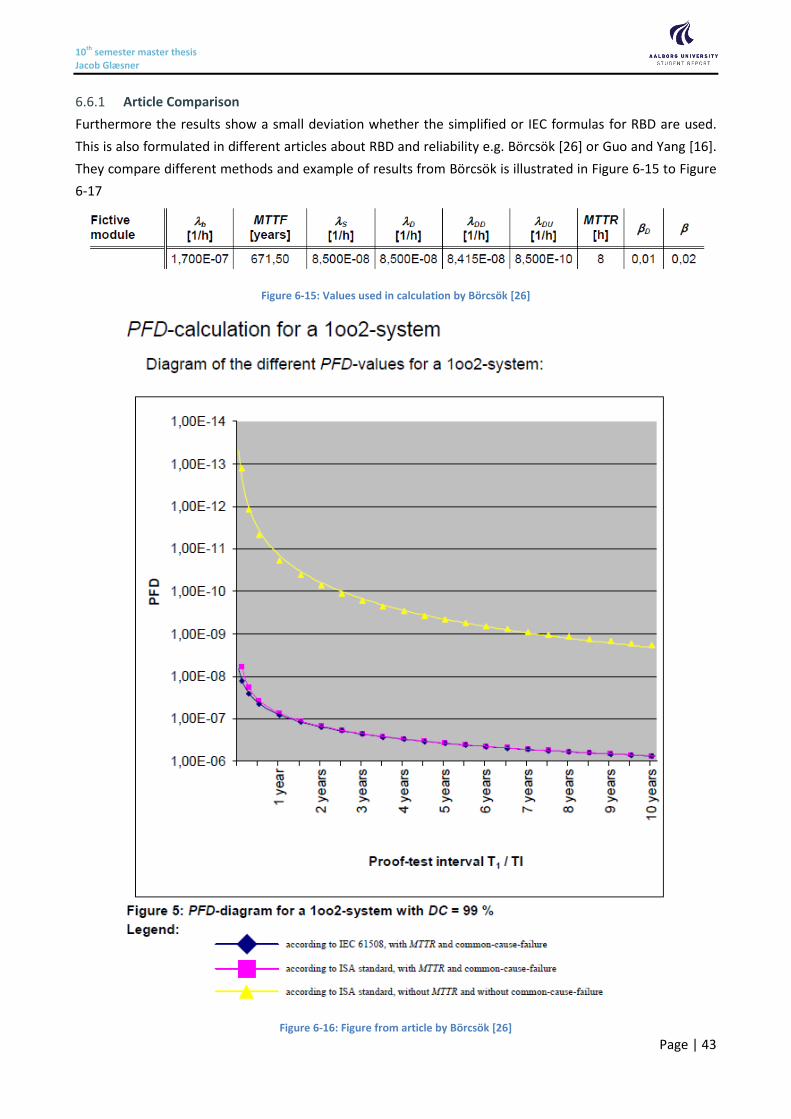
10th semester master thesis Jacob Glæsner
Page | 43
Article Comparison 6.6.1
Furthermore the results show a small deviation whether the simplified or IEC formulas for RBD are used.
This is also formulated in different articles about RBD and reliability e.g. Börcsök [26] or Guo and Yang [16].
They compare different methods and example of results from Börcsök is illustrated in Figure 6-15 to Figure
6-17
Figure 6-15: Values used in calculation by Börcsök [26]
Figure 6-16: Figure from article by Börcsök [26]
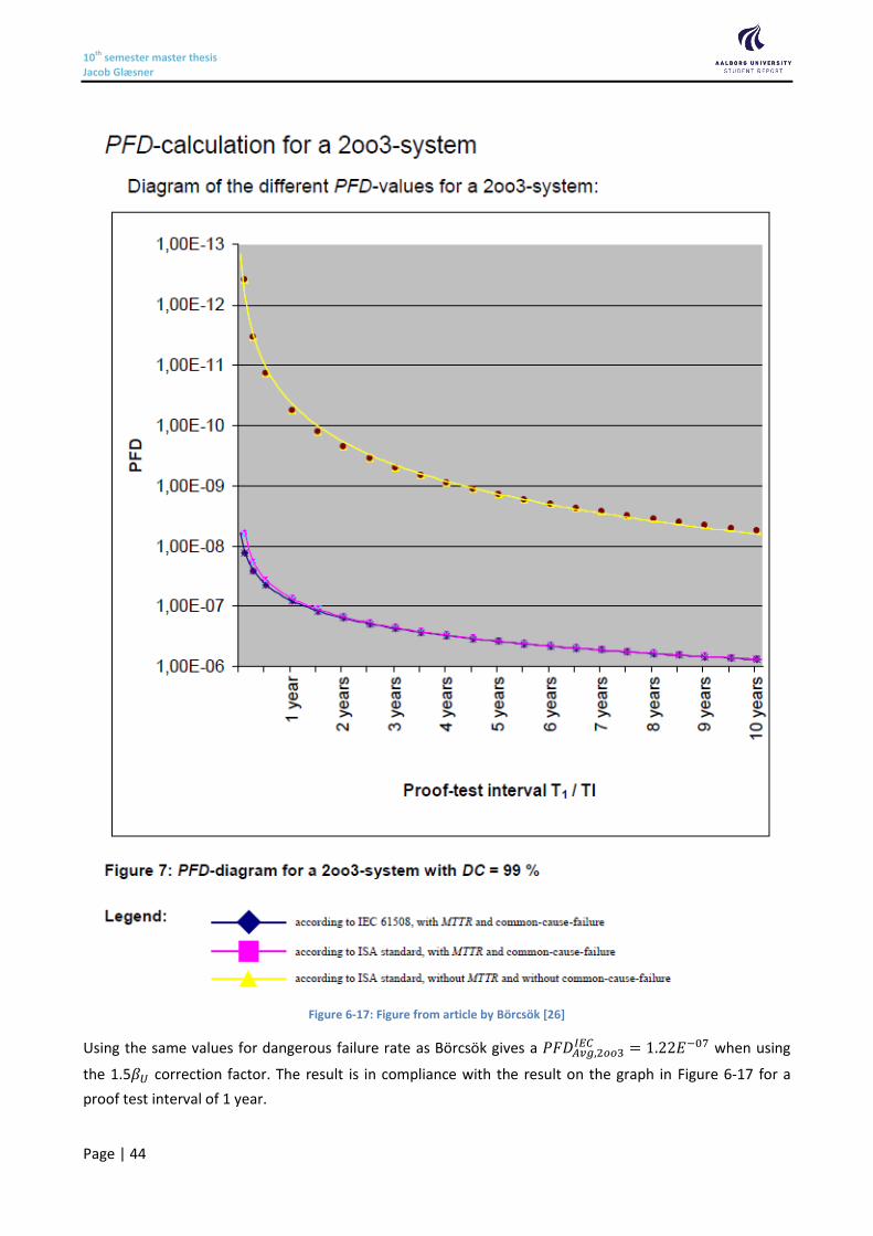
10th semester master thesis Jacob Glæsner
Page | 44
Figure 6-17: Figure from article by Börcsök [26]
Using the same values for dangerous failure rate as Börcsök gives a 𝑃𝐹𝐷𝐴𝑣𝑔,2𝑜𝑜3𝐼𝐸𝐶 = 1.22𝐸−07 when using
the 1.5𝛽𝑈 correction factor. The result is in compliance with the result on the graph in Figure 6-17 for a
proof test interval of 1 year.

10th semester master thesis Jacob Glæsner
Page | 45
Guo and Yang presented the results in Figure 6-18 which for the IEC 61508 columns give the same results if
same values are used in the calculation methods, which are used in this thesis. This validates the results of
this thesis.
Figure 6-18: Results presented by Guo and Yang [16]
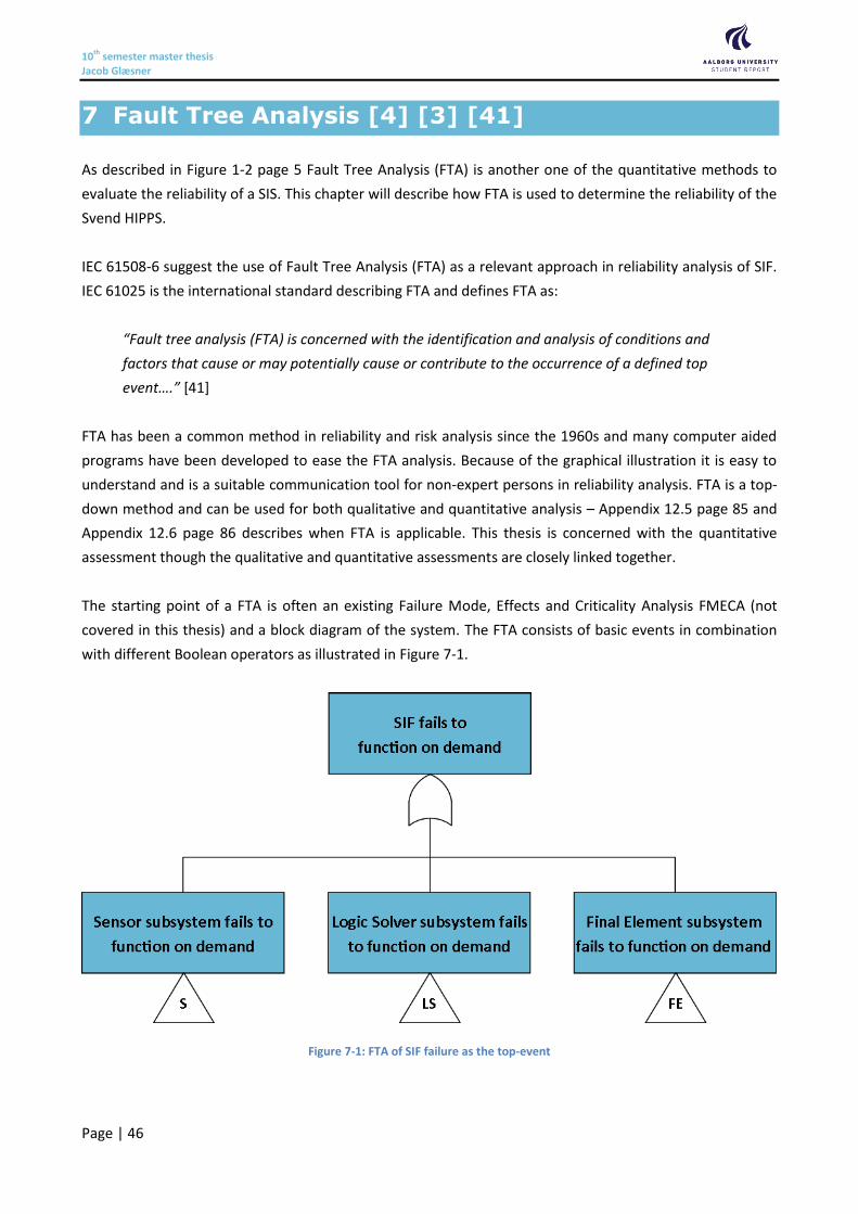
10th semester master thesis Jacob Glæsner
Page | 46
7 Fault Tree Analysis [4] [3] [41]
As described in Figure 1-2 page 5 Fault Tree Analysis (FTA) is another one of the quantitative methods to
evaluate the reliability of a SIS. This chapter will describe how FTA is used to determine the reliability of the
Svend HIPPS.
IEC 61508-6 suggest the use of Fault Tree Analysis (FTA) as a relevant approach in reliability analysis of SIF.
IEC 61025 is the international standard describing FTA and defines FTA as:
“Fault tree analysis (FTA) is concerned with the identification and analysis of conditions and
factors that cause or may potentially cause or contribute to the occurrence of a defined top
event….” [41]
FTA has been a common method in reliability and risk analysis since the 1960s and many computer aided
programs have been developed to ease the FTA analysis. Because of the graphical illustration it is easy to
understand and is a suitable communication tool for non-expert persons in reliability analysis. FTA is a top-
down method and can be used for both qualitative and quantitative analysis – Appendix 12.5 page 85 and
Appendix 12.6 page 86 describes when FTA is applicable. This thesis is concerned with the quantitative
assessment though the qualitative and quantitative assessments are closely linked together.
The starting point of a FTA is often an existing Failure Mode, Effects and Criticality Analysis FMECA (not
covered in this thesis) and a block diagram of the system. The FTA consists of basic events in combination
with different Boolean operators as illustrated in Figure 7-1.
Figure 7-1: FTA of SIF failure as the top-event
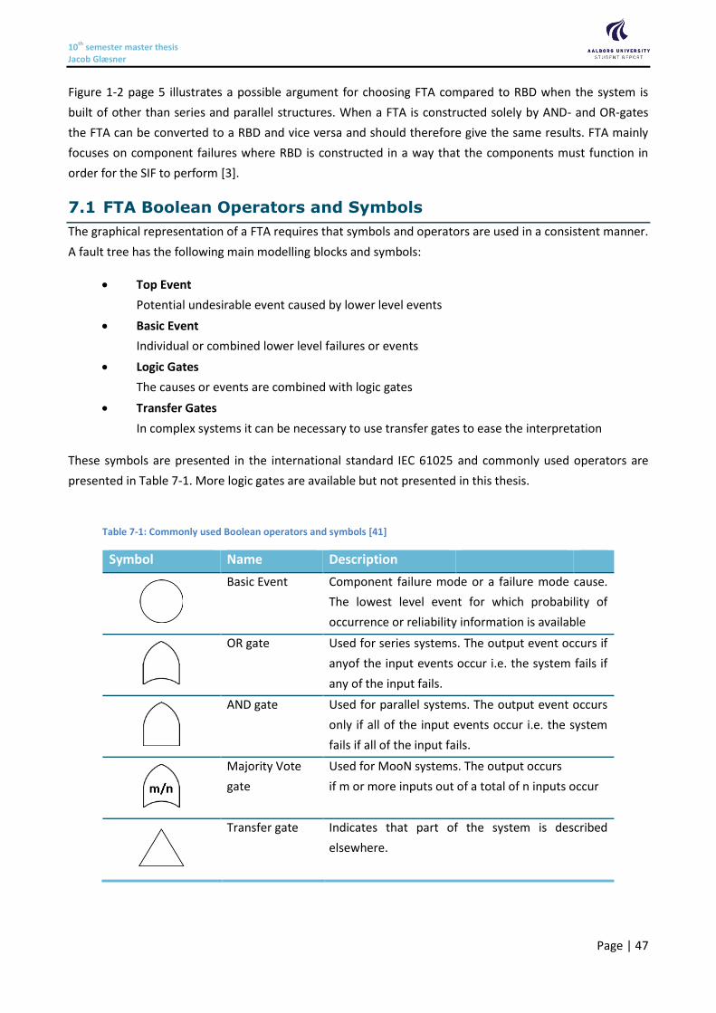
10th semester master thesis Jacob Glæsner
Page | 47
Figure 1-2 page 5 illustrates a possible argument for choosing FTA compared to RBD when the system is
built of other than series and parallel structures. When a FTA is constructed solely by AND- and OR-gates
the FTA can be converted to a RBD and vice versa and should therefore give the same results. FTA mainly
focuses on component failures where RBD is constructed in a way that the components must function in
order for the SIF to perform [3].
7.1 FTA Boolean Operators and Symbols
The graphical representation of a FTA requires that symbols and operators are used in a consistent manner.
A fault tree has the following main modelling blocks and symbols:
Top Event
Potential undesirable event caused by lower level events
Basic Event
Individual or combined lower level failures or events
Logic Gates
The causes or events are combined with logic gates
Transfer Gates
In complex systems it can be necessary to use transfer gates to ease the interpretation
These symbols are presented in the international standard IEC 61025 and commonly used operators are
presented in Table 7-1. More logic gates are available but not presented in this thesis.
Table 7-1: Commonly used Boolean operators and symbols [41]
Symbol Name Description
Basic Event Component failure mode or a failure mode cause.
The lowest level event for which probability of
occurrence or reliability information is available
OR gate Used for series systems. The output event occurs if
anyof the input events occur i.e. the system fails if
any of the input fails.
AND gate Used for parallel systems. The output event occurs
only if all of the input events occur i.e. the system
fails if all of the input fails.
Majority Vote
gate
Used for MooN systems. The output occurs
if m or more inputs out of a total of n inputs occur
Transfer gate Indicates that part of the system is described
elsewhere.
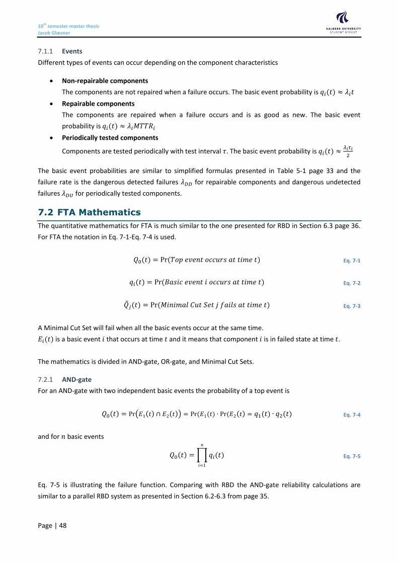
10th semester master thesis Jacob Glæsner
Page | 48
Events 7.1.1
Different types of events can occur depending on the component characteristics
Non-repairable components
The components are not repaired when a failure occurs. The basic event probability is 𝑞𝑖(𝑡) ≈ 𝜆𝑖𝑡
Repairable components
The components are repaired when a failure occurs and is as good as new. The basic event
probability is 𝑞𝑖(𝑡) ≈ 𝜆𝑖𝑀𝑇𝑇𝑅𝑖
Periodically tested components
Components are tested periodically with test interval 𝜏. The basic event probability is 𝑞𝑖(𝑡) ≈𝜆𝑖𝜏𝑖
2
The basic event probabilities are similar to simplified formulas presented in Table 5-1 page 33 and the
failure rate is the dangerous detected failures 𝜆𝐷𝐷 for repairable components and dangerous undetected
failures 𝜆𝐷𝑈 for periodically tested components.
7.2 FTA Mathematics
The quantitative mathematics for FTA is much similar to the one presented for RBD in Section 6.3 page 36.
For FTA the notation in Eq. 7-1-Eq. 7-4 is used.
𝑄0(𝑡) = Pr (𝑇𝑜𝑝 𝑒𝑣𝑒𝑛𝑡 𝑜𝑐𝑐𝑢𝑟𝑠 𝑎𝑡 𝑡𝑖𝑚𝑒 𝑡) Eq. 7-1
𝑞𝑖(𝑡) = Pr (𝐵𝑎𝑠𝑖𝑐 𝑒𝑣𝑒𝑛𝑡 𝑖 𝑜𝑐𝑐𝑢𝑟𝑠 𝑎𝑡 𝑡𝑖𝑚𝑒 𝑡) Eq. 7-2
�̌�𝑗(𝑡) = Pr (𝑀𝑖𝑛𝑖𝑚𝑎𝑙 𝐶𝑢𝑡 𝑆𝑒𝑡 𝑗 𝑓𝑎𝑖𝑙𝑠 𝑎𝑡 𝑡𝑖𝑚𝑒 𝑡) Eq. 7-3
A Minimal Cut Set will fail when all the basic events occur at the same time.
𝐸𝑖(𝑡) is a basic event 𝑖 that occurs at time 𝑡 and it means that component 𝑖 is in failed state at time 𝑡.
The mathematics is divided in AND-gate, OR-gate, and Minimal Cut Sets.
AND-gate 7.2.1
For an AND-gate with two independent basic events the probability of a top event is
𝑄0(𝑡) = Pr(𝐸1(𝑡) ∩ 𝐸2(𝑡)) = Pr (𝐸1(𝑡) ∙ Pr (𝐸2(𝑡) = 𝑞1(𝑡) ∙ 𝑞2(𝑡) Eq. 7-4
and for 𝑛 basic events
𝑄0(𝑡) = ∏𝑞𝑖(𝑡)
𝑛
𝑖=1
Eq. 7-5
Eq. 7-5 is illustrating the failure function. Comparing with RBD the AND-gate reliability calculations are
similar to a parallel RBD system as presented in Section 6.2-6.3 from page 35.

10th semester master thesis Jacob Glæsner
Page | 49
OR-gate 7.2.2
For an OR-gate with two independent basic events the probability of a top event is
𝑄0(𝑡) = Pr(𝐸1(𝑡) ∪ 𝐸2(𝑡)) = Pr (𝐸1(𝑡) + Pr (𝐸2(𝑡) − Pr(𝐸1(𝑡) ∩ 𝐸2(𝑡))
= 𝑞1(𝑡) + 𝑞2(𝑡) − 𝑞1(𝑡) ∙ 𝑞2(𝑡) = 1 − (1 − 𝑞1(𝑡))(1 − 𝑞2(𝑡)) Eq. 7-6
and for 𝑛 basic events
𝑄0(𝑡) = 1 − ∏(1 − 𝑞𝑖(𝑡))
𝑛
𝑖=1
Eq. 7-7
Eq. 7-7 is illustrating the failure function. Comparing with RBD the OR-gate reliability calculations are similar
to a series RBD system as presented in Section 6.2-6.3 from page 35.
Minimal Cut Sets 7.2.3
A cut set is a set of components that by failing puts the system in down state. In a MooN system the
number of minimal cut set can be calculated as
𝑚𝑖𝑛𝑚𝑎𝑙 𝑐𝑢𝑡 𝑠𝑒𝑡 = (𝑛
𝑛 − 𝑚 + 1) Eq. 7-8
The system fails if 𝑛 − 𝑚 + 1 cut sets fail.
When calculating the probability of a minimal cut set occurring in a time interval 𝑡 the main approach is
�̌�𝑗(𝑡) = ∏ 𝑞𝑖(𝑡)
𝑛−𝑚+1
𝑖=1
Eq. 7-9
The use of minimal cut sets for FTA in MooN voted groups lead to a non-conservative answer and must be
multiplied with a correction factor, 𝐶𝐹.
𝐶𝐹 =2𝑘
𝑘 + 1 Eq. 7-10
For a minimal cut set with 𝑘 = 𝑛 − 𝑚 + 1 components
Average Probability of Failure on Demand 7.2.4
After finding the basic event failure function 𝑄0(𝑡) then the average probability of failure on demand can
be calculated.
𝑃𝐹𝐷𝐴𝑣𝑔 =1
𝜏∫ 𝑄0(𝑡)
𝜏
0
𝑑𝑡 Eq. 7-11
Most software programs use the basic event function to calculate the 𝑃𝐹𝐷𝐴𝑣𝑔 [3].
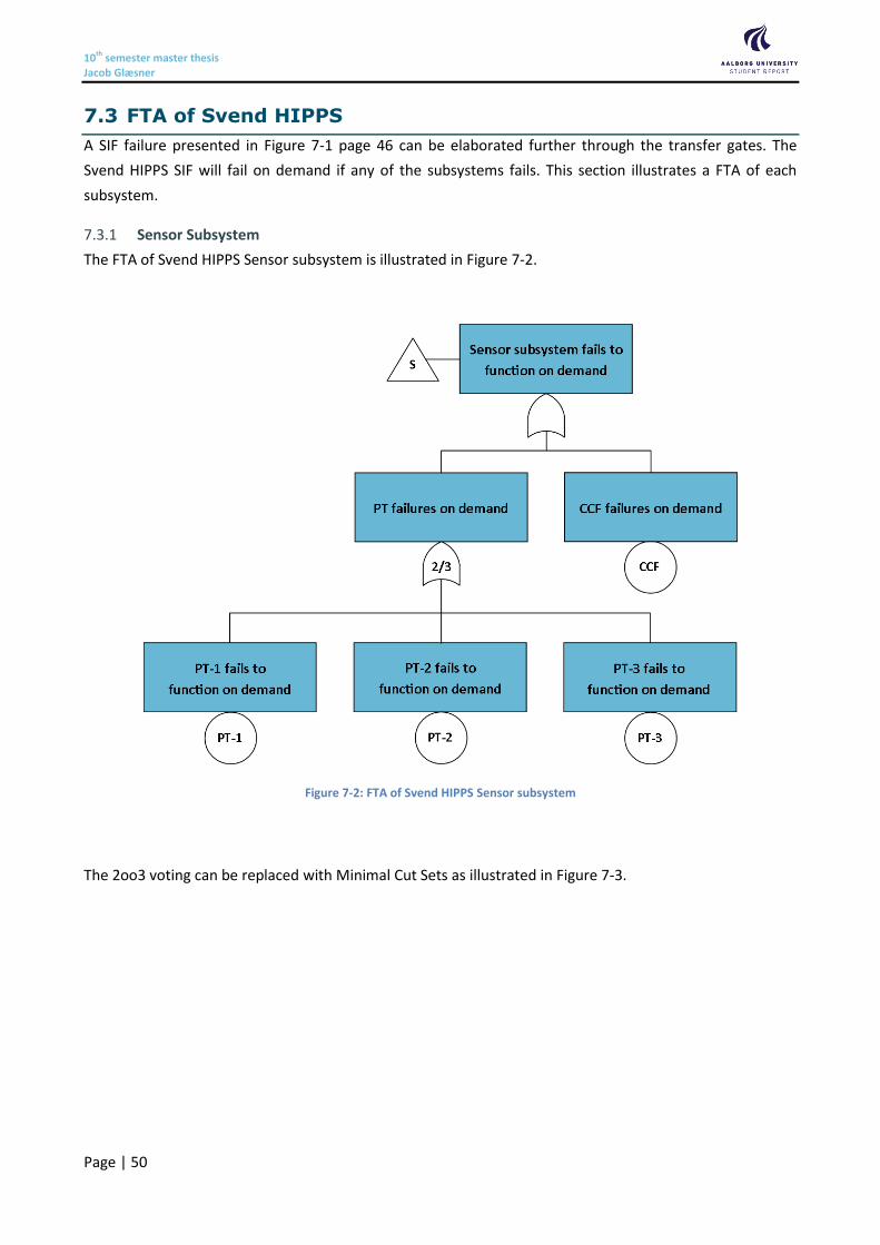
10th semester master thesis Jacob Glæsner
Page | 50
7.3 FTA of Svend HIPPS
A SIF failure presented in Figure 7-1 page 46 can be elaborated further through the transfer gates. The
Svend HIPPS SIF will fail on demand if any of the subsystems fails. This section illustrates a FTA of each
subsystem.
Sensor Subsystem 7.3.1
The FTA of Svend HIPPS Sensor subsystem is illustrated in Figure 7-2.
Figure 7-2: FTA of Svend HIPPS Sensor subsystem
The 2oo3 voting can be replaced with Minimal Cut Sets as illustrated in Figure 7-3.
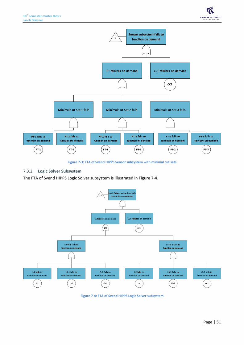
10th semester master thesis Jacob Glæsner
Page | 51
Figure 7-3: FTA of Svend HIPPS Sensor subsystem with minimal cut sets
Logic Solver Subsystem 7.3.2
The FTA of Svend HIPPS Logic Solver subsystem is illustrated in Figure 7-4.
Figure 7-4: FTA of Svend HIPPS Logic Solver subsystem
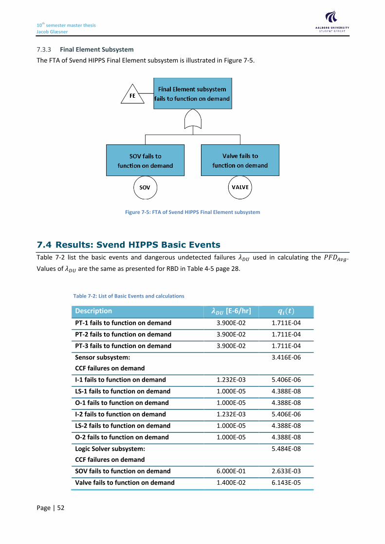
10th semester master thesis Jacob Glæsner
Page | 52
Final Element Subsystem 7.3.3
The FTA of Svend HIPPS Final Element subsystem is illustrated in Figure 7-5.
Figure 7-5: FTA of Svend HIPPS Final Element subsystem
7.4 Results: Svend HIPPS Basic Events
Table 7-2 list the basic events and dangerous undetected failures 𝜆𝐷𝑈 used in calculating the 𝑃𝐹𝐷𝐴𝑣𝑔.
Values of 𝜆𝐷𝑈 are the same as presented for RBD in Table 4-5 page 28.
Table 7-2: List of Basic Events and calculations
Description 𝝀𝑫𝑼 [E-6/hr] 𝒒𝒊(𝒕)
PT-1 fails to function on demand 3.900E-02 1.711E-04
PT-2 fails to function on demand 3.900E-02 1.711E-04
PT-3 fails to function on demand 3.900E-02 1.711E-04
Sensor subsystem:
CCF failures on demand
3.416E-06
I-1 fails to function on demand 1.232E-03 5.406E-06
LS-1 fails to function on demand 1.000E-05 4.388E-08
O-1 fails to function on demand 1.000E-05 4.388E-08
I-2 fails to function on demand 1.232E-03 5.406E-06
LS-2 fails to function on demand 1.000E-05 4.388E-08
O-2 fails to function on demand 1.000E-05 4.388E-08
Logic Solver subsystem:
CCF failures on demand
5.484E-08
SOV fails to function on demand 6.000E-01 2.633E-03
Valve fails to function on demand 1.400E-02 6.143E-05
10th semester master thesis Jacob Glæsner
Page | 53
The CCF values are calculated with Eq. 5-22 page 32.
The basis event probabilities 𝑞𝑖(𝑡) in Table 7-2 are calculated with Eq. 7-12.
𝑞𝑖(𝑡) =𝜆𝐷𝑈,𝑖𝜏𝑖
2+ 𝜆𝐷𝑈,𝑖𝑀𝑇𝑇𝑅 Eq. 7-12
with 𝜏𝑖 = 8760 [ℎ] and 𝑀𝑇𝑇𝑅 = 8 [ℎ] (standard IEC values – other can be used)
Using the basis event probabilities and the FTA Boolean math presented in this chapter to calculate the top
event 𝑄0(𝑡) gives a
𝑃𝐹𝐷𝐴𝑣𝑔,𝑆𝐼𝐹𝐹𝑇𝐴 = 2.71𝐸−03 Eq. 7-13
and
𝑅𝑅𝐹𝑆𝐼𝐹𝐹𝑇𝐴 = 369 𝑆𝐼𝐿𝑆𝐼𝐹
𝐹𝑇𝐴 = 2 Eq. 7-14
The result for FTA is as expected much similar to the one presented for RBD in Section 6.6 page 42.
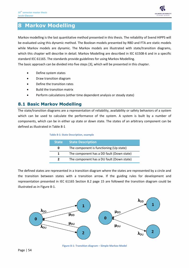
10th semester master thesis Jacob Glæsner
Page | 54
8 Markov Modelling
Markov modelling is the last quantitative method presented in this thesis. The reliability of Svend HIPPS will
be evaluated using this dynamic method. The Boolean models presented by RBD and FTA are static models
while Markov models are dynamic. The Markov models are illustrated with state/transition diagrams,
which this chapter will describe in detail. Markov Modelling are described in IEC 61508-6 and in a specific
standard IEC 61165. The standards provide guidelines for using Markov Modelling.
The basic approach can be divided into five steps [3], which will be presented in this chapter.
Define system states
Draw transition diagram
Define the transition rates
Build the transition matrix
Perform calculations (either time dependent analysis or steady state)
8.1 Basic Markov Modelling
The state/transition diagrams are a representation of reliability, availability or safety behaviors of a system
which can be used to calculate the performance of the system. A system is built by a number of
components, which can be in either up state or down state. The states of an arbitrary component can be
defined as illustrated in Table 8-1
Table 8-1: State Description, example
State State Description
0 The component is functioning (Up state)
1 The component has a DD fault (Down state)
2 The component has a DU fault (Down state)
The defined states are represented in a transition diagram where the states are represented by a circle and
the transition between states with a transition arrow. If the guiding rules for development and
representation presented in IEC 61165 Section 8.2 page 15 are followed the transition diagram could be
illustrated as in Figure 8-1.
Figure 8-1: Transition diagram – Simple Markov Model
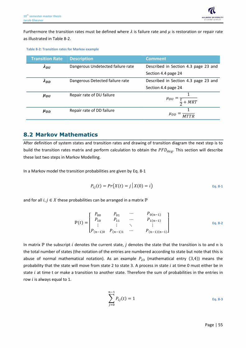
10th semester master thesis Jacob Glæsner
Page | 55
Furthermore the transition rates must be defined where 𝜆 is failure rate and 𝜇 is restoration or repair rate
as illustrated in Table 8-2.
Table 8-2: Transition rates for Markov example
Transition Rate Description Comment
𝝀𝑫𝑼 Dangerous Undetected failure rate Described in Section 4.3 page 23 and
Section 4.4 page 24
𝝀𝑫𝑫 Dangerous Detected failure rate Described in Section 4.3 page 23 and
Section 4.4 page 24
𝝁𝑫𝑼 Repair rate of DU failure 𝜇𝐷𝑈 =
1𝜏2 + 𝑀𝑅𝑇
𝝁𝑫𝑫 Repair rate of DD failure 𝜇𝐷𝐷 =
1
𝑀𝑇𝑇𝑅
8.2 Markov Mathematics
After definition of system states and transition rates and drawing of transition diagram the next step is to
build the transition rates matrix and perform calculation to obtain the 𝑃𝐹𝐷𝐴𝑣𝑔. This section will describe
these last two steps in Markov Modelling.
In a Markov model the transition probabilities are given by Eq. 8-1
𝑃𝑖𝑗(𝑡) = 𝑃𝑟(𝑋(𝑡) = 𝑗│𝑋(0) = 𝑖) Eq. 8-1
and for all 𝑖, 𝑗 ∈ 𝑋 these probabilities can be arranged in a matrix ℙ
ℙ(𝑡) =
[
𝑃00 𝑃01
𝑃10 𝑃11
⋯ 𝑃0(𝑛−1)
⋯ 𝑃1(𝑛−1)
⋮ ⋮𝑃(𝑛−1)0 𝑃(𝑛−1)1
⋱ ⋮ ⋯ 𝑃(𝑛−1)(𝑛−1)]
Eq. 8-2
In matrix ℙ the subscript 𝑖 denotes the current state, 𝑗 denotes the state that the transition is to and 𝑛 is
the total number of states (the notation of the entries are numbered according to state but note that this is
abuse of normal mathematical notation). As an example 𝑃23 (mathematical entry (3,4)) means the
probability that the state will move from state 2 to state 3. A process in state 𝑖 at time 0 must either be in
state 𝑖 at time t or make a transition to another state. Therefore the sum of probabilities in the entries in
row 𝑖 is always equal to 1.
∑ 𝑃𝑖𝑗(𝑡) = 1
𝑛−1
𝑗=0
Eq. 8-3
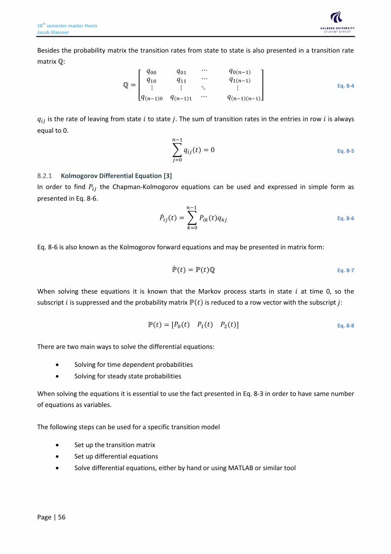
10th semester master thesis Jacob Glæsner
Page | 56
Besides the probability matrix the transition rates from state to state is also presented in a transition rate
matrix ℚ:
ℚ = [
𝑞00 𝑞01
𝑞10 𝑞11
⋯ 𝑞0(𝑛−1) ⋯ 𝑞1(𝑛−1)
⋮ ⋮𝑞(𝑛−1)0 𝑞(𝑛−1)1
⋱ ⋮ ⋯ 𝑞(𝑛−1)(𝑛−1)
] Eq. 8-4
𝑞𝑖𝑗 is the rate of leaving from state 𝑖 to state 𝑗. The sum of transition rates in the entries in row 𝑖 is always
equal to 0.
∑ 𝑞𝑖𝑗(𝑡) = 0
𝑛−1
𝑗=0
Eq. 8-5
Kolmogorov Differential Equation [3] 8.2.1
In order to find 𝑃𝑖𝑗 the Chapman-Kolmogorov equations can be used and expressed in simple form as
presented in Eq. 8-6.
�̇�𝑖𝑗(𝑡) = ∑ 𝑃𝑖𝑘(𝑡)𝑞𝑘𝑗
𝑛−1
𝑘=0
Eq. 8-6
Eq. 8-6 is also known as the Kolmogorov forward equations and may be presented in matrix form:
ℙ̇(𝑡) = ℙ(𝑡)ℚ Eq. 8-7
When solving these equations it is known that the Markov process starts in state 𝑖 at time 0, so the
subscript 𝑖 is suppressed and the probability matrix ℙ(𝑡) is reduced to a row vector with the subscript 𝑗:
ℙ(𝑡) = [𝑃0(𝑡) 𝑃1(𝑡) 𝑃2(𝑡)] Eq. 8-8
There are two main ways to solve the differential equations:
Solving for time dependent probabilities
Solving for steady state probabilities
When solving the equations it is essential to use the fact presented in Eq. 8-3 in order to have same number
of equations as variables.
The following steps can be used for a specific transition model
Set up the transition matrix
Set up differential equations
Solve differential equations, either by hand or using MATLAB or similar tool
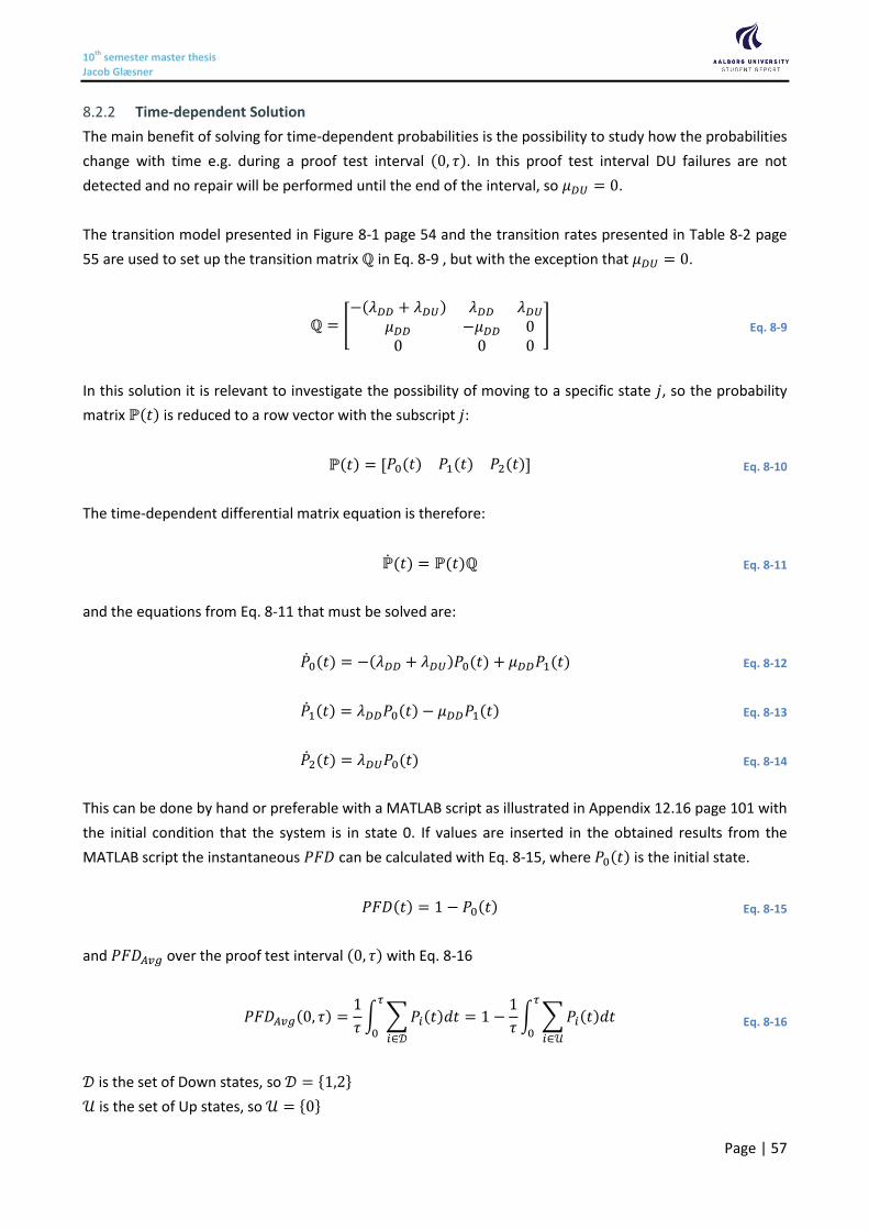
10th semester master thesis Jacob Glæsner
Page | 57
Time-dependent Solution 8.2.2
The main benefit of solving for time-dependent probabilities is the possibility to study how the probabilities
change with time e.g. during a proof test interval (0, 𝜏). In this proof test interval DU failures are not
detected and no repair will be performed until the end of the interval, so 𝜇𝐷𝑈 = 0.
The transition model presented in Figure 8-1 page 54 and the transition rates presented in Table 8-2 page
55 are used to set up the transition matrix ℚ in Eq. 8-9 , but with the exception that 𝜇𝐷𝑈 = 0.
ℚ = [−(𝜆𝐷𝐷 + 𝜆𝐷𝑈) 𝜆𝐷𝐷 𝜆𝐷𝑈
𝜇𝐷𝐷 −𝜇𝐷𝐷 00 0 0
] Eq. 8-9
In this solution it is relevant to investigate the possibility of moving to a specific state 𝑗, so the probability
matrix ℙ(𝑡) is reduced to a row vector with the subscript 𝑗:
ℙ(𝑡) = [𝑃0(𝑡) 𝑃1(𝑡) 𝑃2(𝑡)] Eq. 8-10
The time-dependent differential matrix equation is therefore:
ℙ̇(𝑡) = ℙ(𝑡)ℚ Eq. 8-11
and the equations from Eq. 8-11 that must be solved are:
�̇�0(𝑡) = −(𝜆𝐷𝐷 + 𝜆𝐷𝑈)𝑃0(𝑡) + 𝜇𝐷𝐷𝑃1(𝑡) Eq. 8-12
�̇�1(𝑡) = 𝜆𝐷𝐷𝑃0(𝑡) − 𝜇𝐷𝐷𝑃1(𝑡) Eq. 8-13
�̇�2(𝑡) = 𝜆𝐷𝑈𝑃0(𝑡) Eq. 8-14
This can be done by hand or preferable with a MATLAB script as illustrated in Appendix 12.16 page 101 with
the initial condition that the system is in state 0. If values are inserted in the obtained results from the
MATLAB script the instantaneous 𝑃𝐹𝐷 can be calculated with Eq. 8-15, where 𝑃0(𝑡) is the initial state.
𝑃𝐹𝐷(𝑡) = 1 − 𝑃0(𝑡) Eq. 8-15
and 𝑃𝐹𝐷𝐴𝑣𝑔 over the proof test interval (0, 𝜏) with Eq. 8-16
𝑃𝐹𝐷𝐴𝑣𝑔(0, 𝜏) =1
𝜏∫ ∑𝑃𝑖(𝑡)𝑑𝑡
𝑖∈𝒟
𝜏
0
= 1 −1
𝜏∫ ∑𝑃𝑖(𝑡)𝑑𝑡
𝑖∈𝒰
𝜏
0
Eq. 8-16
𝒟 is the set of Down states, so 𝒟 = {1,2}
𝒰 is the set of Up states, so 𝒰 = {0}
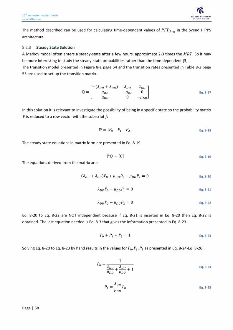
10th semester master thesis Jacob Glæsner
Page | 58
The method described can be used for calculating time-dependent values of 𝑃𝐹𝐷𝐴𝑣𝑔 in the Svend HIPPS
architecture.
Steady State Solution 8.2.3
A Markov model often enters a steady-state after a few hours, approximate 2-3 times the 𝑀𝑅𝑇. So it may
be more interesting to study the steady-state probabilities rather than the time-dependent [3].
The transition model presented in Figure 8-1 page 54 and the transition rates presented in Table 8-2 page
55 are used to set up the transition matrix.
ℚ = [−(𝜆𝐷𝐷 + 𝜆𝐷𝑈) 𝜆𝐷𝐷 𝜆𝐷𝑈
𝜇𝐷𝐷 −𝜇𝐷𝐷 0𝜇𝐷𝑈 0 −𝜇𝐷𝑈
] Eq. 8-17
In this solution it is relevant to investigate the possibility of being in a specific state so the probability matrix
ℙ is reduced to a row vector with the subscript 𝑗:
ℙ = [𝑃0 𝑃1 𝑃2] Eq. 8-18
The steady state equations in matrix form are presented in Eq. 8-19:
ℙℚ = [0] Eq. 8-19
The equations derived from the matrix are:
−(𝜆𝐷𝐷 + 𝜆𝐷𝑈)𝑃0 + 𝜇𝐷𝐷𝑃1 + 𝜇𝐷𝑈𝑃2 = 0 Eq. 8-20
𝜆𝐷𝐷𝑃0 − 𝜇𝐷𝐷𝑃1 = 0 Eq. 8-21
𝜆𝐷𝑈𝑃0 − 𝜇𝐷𝑈𝑃2 = 0 Eq. 8-22
Eq. 8-20 to Eq. 8-22 are NOT independent because if Eq. 8-21 is inserted in Eq. 8-20 then Eq. 8-22 is
obtained. The last equation needed is Eq. 8-3 that gives the information presented in Eq. 8-23.
𝑃0 + 𝑃1 + 𝑃2 = 1 Eq. 8-23
Solving Eq. 8-20 to Eq. 8-23 by hand results in the values for 𝑃0, 𝑃1, 𝑃2 as presented in Eq. 8-24-Eq. 8-26:
𝑃0 =1
𝜆𝐷𝐷𝜇𝐷𝐷
+𝜆𝐷𝑈𝜇𝐷𝑈
+ 1
Eq. 8-24
𝑃1 =𝜆𝐷𝐷
𝜇𝐷𝐷𝑃0 Eq. 8-25
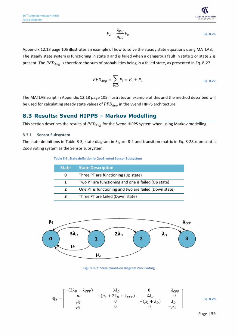
10th semester master thesis Jacob Glæsner
Page | 59
𝑃2 =𝜆𝐷𝑈
𝜇𝐷𝑈𝑃0 Eq. 8-26
Appendix 12.18 page 105 illustrates an example of how to solve the steady state equations using MATLAB.
The steady state system is functioning in state 0 and is failed when a dangerous fault in state 1 or state 2 is
present. The 𝑃𝐹𝐷𝐴𝑣𝑔 is therefore the sum of probabilities being in a failed state, as presented in Eq. 8-27.
𝑃𝐹𝐷𝐴𝑣𝑔 = ∑𝑃𝑖
𝑖∈𝒟
= 𝑃1 + 𝑃2 Eq. 8-27
The MATLAB script in Appendix 12.18 page 105 illustrates an example of this and the method described will
be used for calculating steady state values of 𝑃𝐹𝐷𝐴𝑣𝑔 in the Svend HIPPS architecture.
8.3 Results: Svend HIPPS – Markov Modelling
This section describes the results of 𝑃𝐹𝐷𝐴𝑣𝑔 for the Svend HIPPS system when using Markov modelling.
Sensor Subsystem 8.3.1
The state definitions in Table 8-3, state diagram in Figure 8-2 and transition matrix in Eq. 8-28 represent a
2oo3 voting system as the Sensor subsystem.
Table 8-3: State definition in 2oo3 voted Sensor Subsystem
State State Description
0 Three PT are functioning (Up state)
1 Two PT are functioning and one is failed (Up state)
2 One PT is functioning and two are failed (Down state)
3 Three PT are failed (Down state)
Figure 8-2: State transition diagram 2oo3 voting
ℚ𝑆 =
[ −(3𝜆𝐷 + 𝜆𝐶𝐹𝐹) 3𝜆𝐷
𝜇1 −(𝜇1 + 2𝜆𝐷 + 𝜆𝐶𝐹𝐹) 0 𝜆𝐶𝐹𝐹
2𝜆𝐷 0
𝜇2 0 𝜇3 0
−(𝜇2 + 𝜆𝐷) 𝜆𝐷 0 −𝜇3 ]
Eq. 8-28
10th semester master thesis Jacob Glæsner
Page | 60
with the failure rates from Table 4-5 page 28, 𝛽𝑢 = 0.02 and 𝑀𝑇𝑇𝑅 = 𝑀𝑇𝑅 = 8 ℎ𝑜𝑢𝑟𝑠 and 𝜏 =
8760 ℎ𝑜𝑢𝑟𝑠
𝜆𝐷 = 𝜆𝐷𝑈 = 3.90𝐸−08 𝜇1 = 𝜇2 = 𝜇3 = 𝜇𝐷𝑈 =1
𝜏2
+ 𝑀𝑅𝑇
𝜆𝐶𝐹𝐹 = 𝛽𝑢𝜆𝐷𝑈
Steady State solution
In the steady state solution it is relevant to investigate the possibility of being in a specific state so the
probability matrix ℙ is defined as:
ℙ = [𝑃0 𝑃1 𝑃2 𝑃3] Eq. 8-29
The steady state equations in matrix form are presented:
ℙℚ𝑆 = [0] Eq. 8-30
Equations in Eq. 8-30 are NOT independent so Eq. 8-3 page 55 must be used together with Eq. 8-30.
Appendix 12.17 page 103 presents a MATLAB script to the steady state solution of the 2oo3 voting of the
Sensor subsystem. Running the script results in the 𝑃𝐹𝐷𝐴𝑣𝑔 value in Eq. 8-31, which is the sum of
probabilities being in a failed state, 𝒟 = {2,3}.
𝑃𝐹𝐷𝐴𝑣𝑔,𝑆𝑀𝑎𝑟𝑘𝑜𝑣 = ∑𝑃𝑖
𝑖∈𝒟
= 𝑃2 + 𝑃3 = 3.596𝐸−06 Eq. 8-31
It is important to mention that the result in Eq. 8-31 is obtained without 𝐷𝐷 failures and 𝑀𝑇𝑇𝑅 of these
components. A 27x27 transition matrix must be built in order to account for both 𝐷𝐷 and 𝐷𝑈 failures but
this has been omitted from this thesis. Table 12-4 in Appendix 12.20 page 109 illustrates the State
Definitions of the three components in the 2oo3 voting in the Sensor subsystem. Using the definitions in
Table 12-4 will assumedly results in a more precise 𝑃𝐹𝐷𝐴𝑣𝑔,𝑆𝑀𝑎𝑟𝑘𝑜𝑣 value.
Time-dependent solution
See MATLAB script Appendix 12.16 page 101. The time-dependent solution is not elaborated further as it is
expected to give the same result for the same proof test interval. The MATLAB script takes a while to run
and execute, so the steady state solution is preferable.
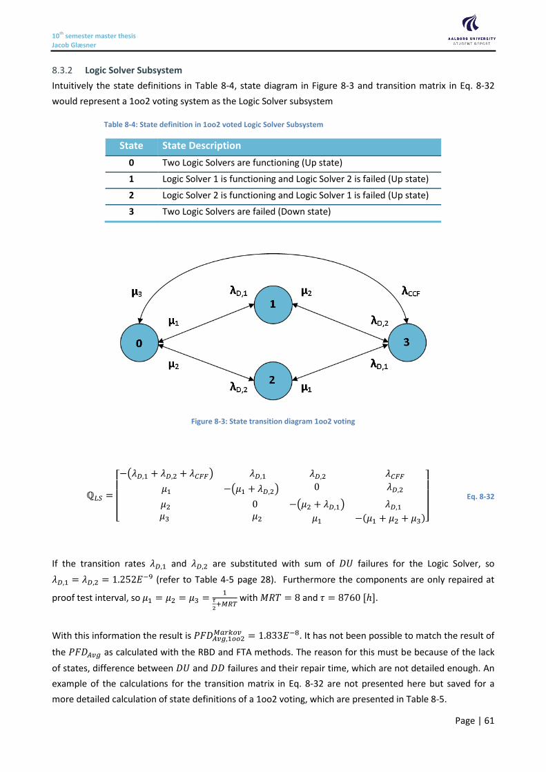
10th semester master thesis Jacob Glæsner
Page | 61
Logic Solver Subsystem 8.3.2
Intuitively the state definitions in Table 8-4, state diagram in Figure 8-3 and transition matrix in Eq. 8-32
would represent a 1oo2 voting system as the Logic Solver subsystem
Table 8-4: State definition in 1oo2 voted Logic Solver Subsystem
State State Description
0 Two Logic Solvers are functioning (Up state)
1 Logic Solver 1 is functioning and Logic Solver 2 is failed (Up state)
2 Logic Solver 2 is functioning and Logic Solver 1 is failed (Up state)
3 Two Logic Solvers are failed (Down state)
Figure 8-3: State transition diagram 1oo2 voting
ℚ𝐿𝑆 =
[ −(𝜆𝐷,1 + 𝜆𝐷,2 + 𝜆𝐶𝐹𝐹) 𝜆𝐷,1
𝜇1 −(𝜇1 + 𝜆𝐷,2)
𝜆𝐷,2 𝜆𝐶𝐹𝐹
0 𝜆𝐷,2
𝜇2 0 𝜇3 𝜇2
−(𝜇2 + 𝜆𝐷,1) 𝜆𝐷,1
𝜇1 −(𝜇1 + 𝜇2 + 𝜇3)]
Eq. 8-32
If the transition rates 𝜆𝐷,1 and 𝜆𝐷,2 are substituted with sum of 𝐷𝑈 failures for the Logic Solver, so
𝜆𝐷,1 = 𝜆𝐷,2 = 1.252𝐸−9 (refer to Table 4-5 page 28). Furthermore the components are only repaired at
proof test interval, so 𝜇1 = 𝜇2 = 𝜇3 =1
𝜏
2+𝑀𝑅𝑇
with 𝑀𝑅𝑇 = 8 and 𝜏 = 8760 [ℎ].
With this information the result is 𝑃𝐹𝐷𝐴𝑣𝑔,1𝑜𝑜2𝑀𝑎𝑟𝑘𝑜𝑣 = 1.833𝐸−8. It has not been possible to match the result of
the 𝑃𝐹𝐷𝐴𝑣𝑔 as calculated with the RBD and FTA methods. The reason for this must be because of the lack
of states, difference between 𝐷𝑈 and 𝐷𝐷 failures and their repair time, which are not detailed enough. An
example of the calculations for the transition matrix in Eq. 8-32 are not presented here but saved for a
more detailed calculation of state definitions of a 1oo2 voting, which are presented in Table 8-5.
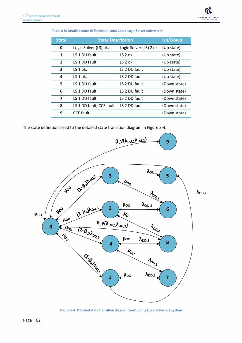
10th semester master thesis Jacob Glæsner
Page | 62
Table 8-5: Detailed state definition in 1oo2 voted Logic Solver Subsystem
State State Description Up/Down
0 Logic Solver (LS) ok, Logic Solver (LS) 2 ok (Up state)
1 LS 1 DU fault, LS 2 ok (Up state)
2 LS 1 DD fault, LS 2 ok (Up state)
3 LS 1 ok, LS 2 DU fault (Up state)
4 LS 1 ok, LS 2 DD fault (Up state)
5 LS 1 DU fault LS 2 DU fault (Down state)
6 LS 1 DD fault, LS 2 DU fault (Down state)
7 LS 1 DU fault, LS 2 DD fault (Down state)
8 LS 1 DD fault, CCF fault LS 2 DD fault (Down state)
9 CCF fault (Down state)
The state definitions lead to the detailed state transition diagram in Figure 8-4.
Figure 8-4: Detailed state transition diagram 1oo2 voting Logic Solver subsystem
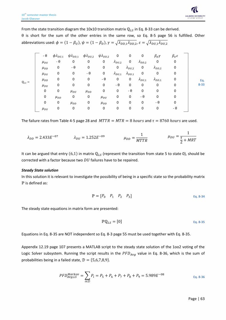
10th semester master thesis Jacob Glæsner
Page | 63
From the state transition diagram the 10x10 transition matrix ℚ𝐿𝑆 in Eq. 8-33 can be derived.
θ is short for the sum of the other entries in the same row, so Eq. 8-5 page 56 is fulfilled. Other
abbreviations used: 𝜙 = (1 − 𝛽𝑈), 𝜓 = (1 − 𝛽𝐷), 𝛾 = √𝜆𝐷𝐷,1𝜆𝐷𝐷,2, 𝜀 = √𝜆𝐷𝑈,1𝜆𝐷𝑈,2
ℚ𝐿𝑆 =
- θ 𝜙𝜆𝐷𝑈,1 𝜓𝜆𝐷𝐷,1 𝜙𝜆𝐷𝑈,2 𝜓𝜆𝐷𝐷,2 0 0 0 𝛽𝐷𝛾 𝛽𝑈𝜀
𝜇𝐷𝑈 - θ 0 0 0 𝜆𝐷𝑈,2 0 𝜆𝐷𝐷,2 0 0
𝜇𝐷𝐷 0 - θ 0 0 0 𝜆𝐷𝑈,2 0 𝜆𝐷𝐷,2 0
𝜇𝐷𝑈 0 0 - θ 0 𝜆𝐷𝑈,1 𝜆𝐷𝐷,1 0 0 0
𝜇𝐷𝐷 0 0 0 - θ 0 0 𝜆𝐷𝑈,1 𝜆𝐷𝐷,1 0
𝜇𝐷𝑈 0 0 0 0 - θ 0 0 0 0
0 0 𝜇𝐷𝑈 𝜇𝐷𝐷 0 0 - θ 0 0 0
0 𝜇𝐷𝐷 0 0 𝜇𝐷𝑈 0 0 - θ 0 0
0 0 𝜇𝐷𝐷 0 𝜇𝐷𝐷 0 0 0 - θ 0
𝜇𝐷𝑈 0 0 0 0 0 0 0 0 - θ
Eq. 8-33
The failure rates from Table 4-5 page 28 and 𝑀𝑇𝑇𝑅 = 𝑀𝑇𝑅 = 8 ℎ𝑜𝑢𝑟𝑠 and 𝜏 = 8760 ℎ𝑜𝑢𝑟𝑠 are used.
𝜆𝐷𝐷 = 2.433𝐸−07 𝜆𝐷𝑈 = 1.252𝐸−09 𝜇𝐷𝐷 =1
𝑀𝑇𝑇𝑅 𝜇𝐷𝑈 =
1𝜏2 + 𝑀𝑅𝑇
It can be argued that entry (6,1) in matrix ℚ𝐿𝑆 (represent the transition from state 5 to state 0), should be
corrected with a factor because two 𝐷𝑈 failures have to be repaired.
Steady State solution
In this solution it is relevant to investigate the possibility of being in a specific state so the probability matrix
ℙ is defined as:
ℙ = [𝑃0 𝑃1 𝑃2 𝑃3] Eq. 8-34
The steady state equations in matrix form are presented:
ℙℚ𝐿𝑆 = [0] Eq. 8-35
Equations in Eq. 8-35 are NOT independent so Eq. 8-3 page 55 must be used together with Eq. 8-35.
Appendix 12.19 page 107 presents a MATLAB script to the steady state solution of the 1oo2 voting of the
Logic Solver subsystem. Running the script results in the 𝑃𝐹𝐷𝐴𝑣𝑔 value in Eq. 8-36, which is the sum of
probabilities being in a failed state, 𝒟 = {5,6,7,8,9}.
𝑃𝐹𝐷𝐴𝑣𝑔,𝐿𝑆𝑀𝑎𝑟𝑘𝑜𝑣 = ∑𝑃𝑖
𝑖∈𝒟
= 𝑃5 + 𝑃6 + 𝑃7 + 𝑃8 + 𝑃9 = 5.989𝐸−08 Eq. 8-36
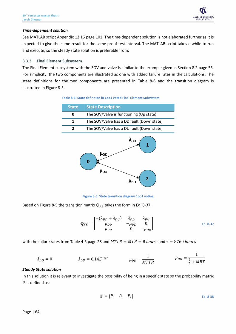
10th semester master thesis Jacob Glæsner
Page | 64
Time-dependent solution
See MATLAB script Appendix 12.16 page 101. The time-dependent solution is not elaborated further as it is
expected to give the same result for the same proof test interval. The MATLAB script takes a while to run
and execute, so the steady state solution is preferable from.
Final Element Subsystem 8.3.3
The Final Element subsystem with the SOV and valve is similar to the example given in Section 8.2 page 55.
For simplicity, the two components are illustrated as one with added failure rates in the calculations. The
state definitions for the two components are presented in Table 8-6 and the transition diagram is
illustrated in Figure 8-5.
Table 8-6: State definition in 1oo1 voted Final Element Subsystem
State State Description
0 The SOV/Valve is functioning (Up state)
1 The SOV/Valve has a DD fault (Down state)
2 The SOV/Valve has a DU fault (Down state)
Figure 8-5: State transition diagram 1oo1 voting
Based on Figure 8-5 the transition matrix ℚ𝐹𝐸 takes the form in Eq. 8-37.
ℚ𝐹𝐸 = [−(𝜆𝐷𝐷 + 𝜆𝐷𝑈) 𝜆𝐷𝐷 𝜆𝐷𝑈
𝜇𝐷𝐷 −𝜇𝐷𝐷 0𝜇𝐷𝑈 0 −𝜇𝐷𝑈
] Eq. 8-37
with the failure rates from Table 4-5 page 28 and 𝑀𝑇𝑇𝑅 = 𝑀𝑇𝑅 = 8 ℎ𝑜𝑢𝑟𝑠 and 𝜏 = 8760 ℎ𝑜𝑢𝑟𝑠
𝜆𝐷𝐷 = 0 𝜆𝐷𝑈 = 6.14𝐸−07 𝜇𝐷𝐷 =1
𝑀𝑇𝑇𝑅 𝜇𝐷𝑈 =
1𝜏2 + 𝑀𝑅𝑇
Steady State solution
In this solution it is relevant to investigate the possibility of being in a specific state so the probability matrix
ℙ is defined as:
ℙ = [𝑃0 𝑃1 𝑃2] Eq. 8-38
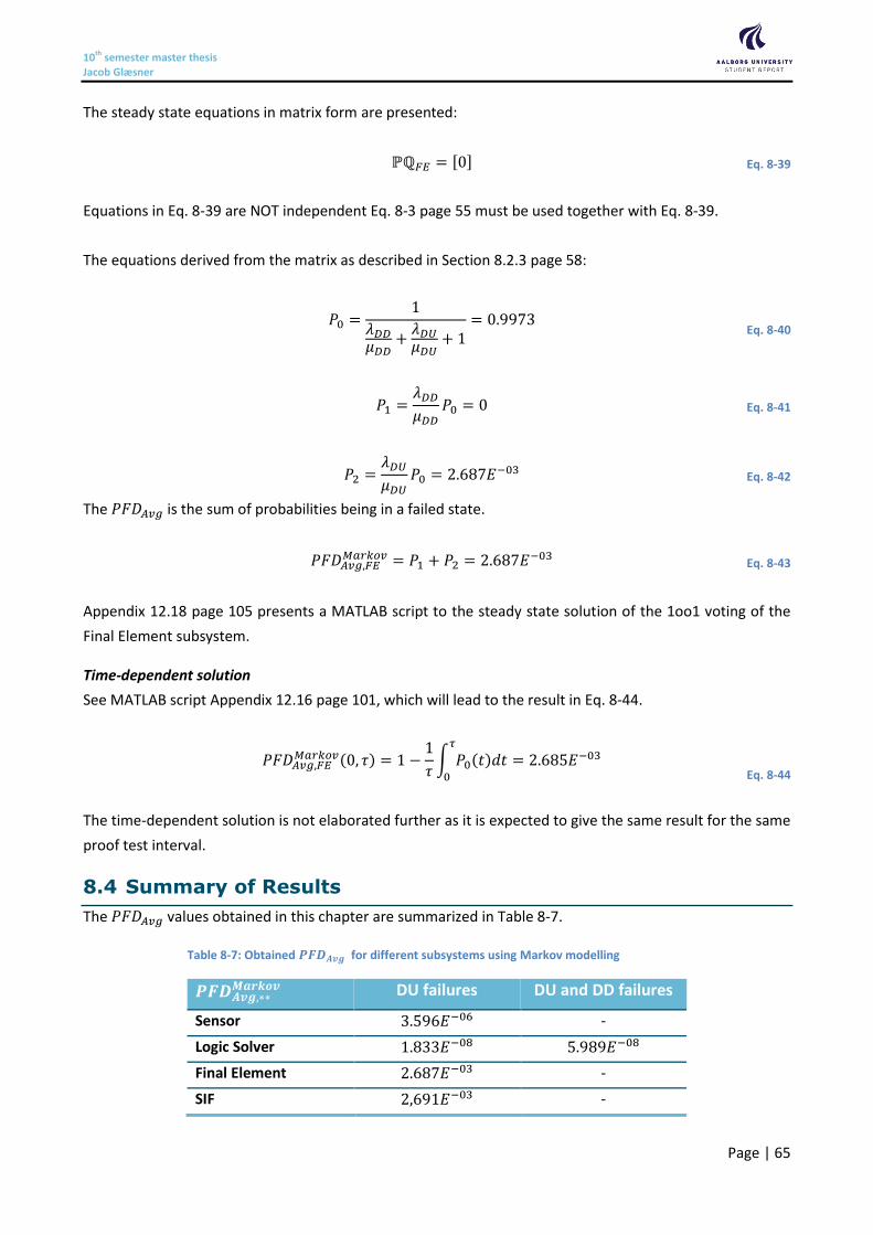
10th semester master thesis Jacob Glæsner
Page | 65
The steady state equations in matrix form are presented:
ℙℚ𝐹𝐸 = [0] Eq. 8-39
Equations in Eq. 8-39 are NOT independent Eq. 8-3 page 55 must be used together with Eq. 8-39.
The equations derived from the matrix as described in Section 8.2.3 page 58:
𝑃0 =1
𝜆𝐷𝐷𝜇𝐷𝐷
+𝜆𝐷𝑈𝜇𝐷𝑈
+ 1= 0.9973
Eq. 8-40
𝑃1 =𝜆𝐷𝐷
𝜇𝐷𝐷𝑃0 = 0 Eq. 8-41
𝑃2 =𝜆𝐷𝑈
𝜇𝐷𝑈𝑃0 = 2.687𝐸−03 Eq. 8-42
The 𝑃𝐹𝐷𝐴𝑣𝑔 is the sum of probabilities being in a failed state.
𝑃𝐹𝐷𝐴𝑣𝑔,𝐹𝐸𝑀𝑎𝑟𝑘𝑜𝑣 = 𝑃1 + 𝑃2 = 2.687𝐸−03 Eq. 8-43
Appendix 12.18 page 105 presents a MATLAB script to the steady state solution of the 1oo1 voting of the
Final Element subsystem.
Time-dependent solution
See MATLAB script Appendix 12.16 page 101, which will lead to the result in Eq. 8-44.
𝑃𝐹𝐷𝐴𝑣𝑔,𝐹𝐸
𝑀𝑎𝑟𝑘𝑜𝑣(0, 𝜏) = 1 −1
𝜏∫ 𝑃0(𝑡)𝑑𝑡
𝜏
0
= 2.685𝐸−03
Eq. 8-44
The time-dependent solution is not elaborated further as it is expected to give the same result for the same
proof test interval.
8.4 Summary of Results
The 𝑃𝐹𝐷𝐴𝑣𝑔 values obtained in this chapter are summarized in Table 8-7.
Table 8-7: Obtained 𝑷𝑭𝑫𝑨𝒗𝒈 for different subsystems using Markov modelling
𝑷𝑭𝑫𝑨𝒗𝒈,∗∗𝑴𝒂𝒓𝒌𝒐𝒗 DU failures DU and DD failures
Sensor 3.596𝐸−06 -
Logic Solver 1.833𝐸−08 5.989𝐸−08
Final Element 2.687𝐸−03 -
SIF 2,691𝐸−03 -
10th semester master thesis Jacob Glæsner
Page | 66
The value for the Final Element is placed under 𝐷𝑈 failures as no 𝐷𝐷 failures where available for the Final
Element. None of the calculations, whether it was RBD or FTA, have used 𝐷𝐷 failures for the Final Element
subsystem. The results are also based on a sum of the failure rates in the series connected systems.
Using the Markov modelling presented in this chapter gives a
𝑃𝐹𝐷𝐴𝑣𝑔,𝑆𝐼𝐹𝑀𝑎𝑟𝑘𝑜𝑣 = 2.69𝐸−03 Eq. 8-45
and
𝑅𝑅𝐹𝑆𝐼𝐹𝑀𝑎𝑟𝑘𝑜𝑣 = 370 𝑆𝐼𝐿𝑆𝐼𝐹
𝑀𝑎𝑟𝑘𝑜𝑣 = 2 Eq. 8-46
The result for Markov modelling is as expected much similar to the one presented for RBD in Section 6.6
page 42. The paper by Börcsök et al. [28] and the paper by Hildebrandt [24] give a general introduction to
Markov modelling and examples of 1oo1 and 1oo2 architecture models. They conclude that using Markov
modelling is in accordance with the values obtained from IEC 61508-6 formulas, which is confirmed in the
results in Eq. 8-45 and Eq. 8-46. They also conclude that the number of states can rapidly increase
depending on the details needed in the model, which will make the model more complex. This was also
shown in this thesis by the number of states needed for result for 𝐷𝑈 and 𝐷𝐷 failures for 2oo3 (Table 12-4
page 109) and 1oo2 (Table 8-5 page 62) systems.
Guo and Yang [17] also describes how explosively the size of Markov models can increase as the system
becomes a little more complicated. They have developed a flowchart for generating a Markov model and a
computer program to automatically realize the technique they present in their paper.
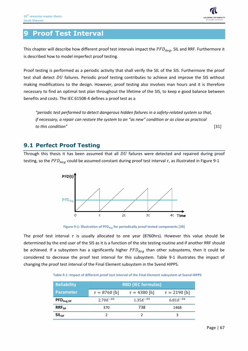
10th semester master thesis Jacob Glæsner
Page | 67
9 Proof Test Interval
This chapter will describe how different proof test intervals impact the 𝑃𝐹𝐷𝐴𝑣𝑔, SIL and RRF. Furthermore it
is described how to model imperfect proof testing.
Proof testing is performed as a periodic activity that shall verify the SIL of the SIS. Furthermore the proof
test shall detect 𝐷𝑈 failures. Periodic proof testing contributes to achieve and improve the SIS without
making modifications to the design. However, proof testing also involves man hours and it is therefore
necessary to find an optimal test plan throughout the lifetime of the SIS, to keep e good balance between
benefits and costs. The IEC 61508-4 defines a proof test as a
“periodic test performed to detect dangerous hidden failures in a safety-related system so that,
if necessary, a repair can restore the system to an “as new” condition or as close as practical
to this condition” [31]
9.1 Perfect Proof Testing
Through this thesis it has been assumed that all 𝐷𝑈 failures were detected and repaired during proof
testing, so the 𝑃𝐹𝐷𝐴𝑣𝑔 could be assumed constant during proof test interval 𝜏, as illustrated in Figure 9-1
Figure 9-1: Illustration of PFDAvg for periodically proof-tested components [39]
The proof test interval 𝜏 is usually allocated to one year (8760hrs). However this value should be
determined by the end user of the SIS as it is a function of the site testing routine and if another RRF should
be achieved. If a subsystem has a significantly higher 𝑃𝐹𝐷𝐴𝑣𝑔 than other subsystems, then it could be
considered to decrease the proof test interval for this subsystem. Table 9-1 illustrates the impact of
changing the proof test interval of the Final Element subsystem in the Svend HIPPS.
Table 9-1: Impact of different proof test interval of the Final Element subsystem at Svend HIPPS
Reliability
Parameter
RBD (IEC formulas)
𝜏 = 8760 [h] 𝜏 = 4380 [h] 𝜏 = 2190 [h]
PFDAvg,SIF 2.70𝐸−03 1.35𝐸−03 6.81𝐸−04
RRFSIF 370 738 1468
SILSIF 2 2 3
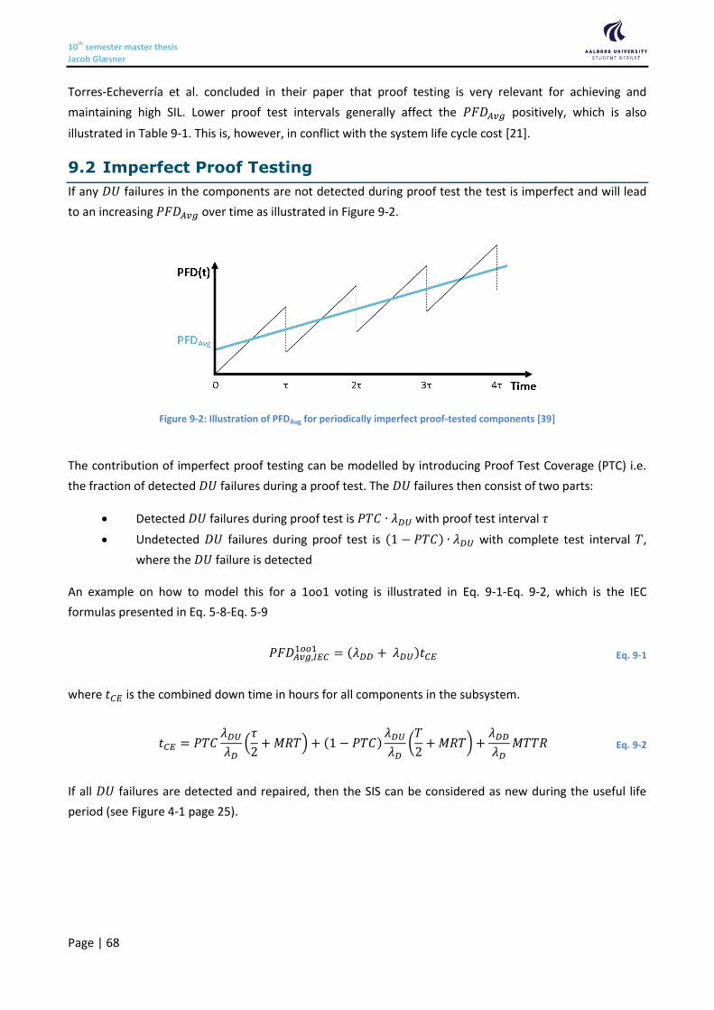
10th semester master thesis Jacob Glæsner
Page | 68
Torres-Echeverría et al. concluded in their paper that proof testing is very relevant for achieving and
maintaining high SIL. Lower proof test intervals generally affect the 𝑃𝐹𝐷𝐴𝑣𝑔 positively, which is also
illustrated in Table 9-1. This is, however, in conflict with the system life cycle cost [21].
9.2 Imperfect Proof Testing
If any 𝐷𝑈 failures in the components are not detected during proof test the test is imperfect and will lead
to an increasing 𝑃𝐹𝐷𝐴𝑣𝑔 over time as illustrated in Figure 9-2.
Figure 9-2: Illustration of PFDAvg for periodically imperfect proof-tested components [39]
The contribution of imperfect proof testing can be modelled by introducing Proof Test Coverage (PTC) i.e.
the fraction of detected 𝐷𝑈 failures during a proof test. The 𝐷𝑈 failures then consist of two parts:
Detected 𝐷𝑈 failures during proof test is 𝑃𝑇𝐶 ∙ 𝜆𝐷𝑈 with proof test interval 𝜏
Undetected 𝐷𝑈 failures during proof test is (1 − 𝑃𝑇𝐶) ∙ 𝜆𝐷𝑈 with complete test interval 𝑇,
where the 𝐷𝑈 failure is detected
An example on how to model this for a 1oo1 voting is illustrated in Eq. 9-1-Eq. 9-2, which is the IEC
formulas presented in Eq. 5-8-Eq. 5-9
𝑃𝐹𝐷𝐴𝑣𝑔,𝐼𝐸𝐶1𝑜𝑜1 = (𝜆𝐷𝐷 + 𝜆𝐷𝑈)𝑡𝐶𝐸 Eq. 9-1
where 𝑡𝐶𝐸 is the combined down time in hours for all components in the subsystem.
𝑡𝐶𝐸 = 𝑃𝑇𝐶𝜆𝐷𝑈
𝜆𝐷(𝜏
2+ 𝑀𝑅𝑇) + (1 − 𝑃𝑇𝐶)
𝜆𝐷𝑈
𝜆𝐷(𝑇
2+ 𝑀𝑅𝑇) +
𝜆𝐷𝐷
𝜆𝐷𝑀𝑇𝑇𝑅 Eq. 9-2
If all 𝐷𝑈 failures are detected and repaired, then the SIS can be considered as new during the useful life
period (see Figure 4-1 page 25).
10th semester master thesis Jacob Glæsner
Page | 69
Concluding
Section

10th semester master thesis Jacob Glæsner
Page | 70
(This page is intentionally left blank)
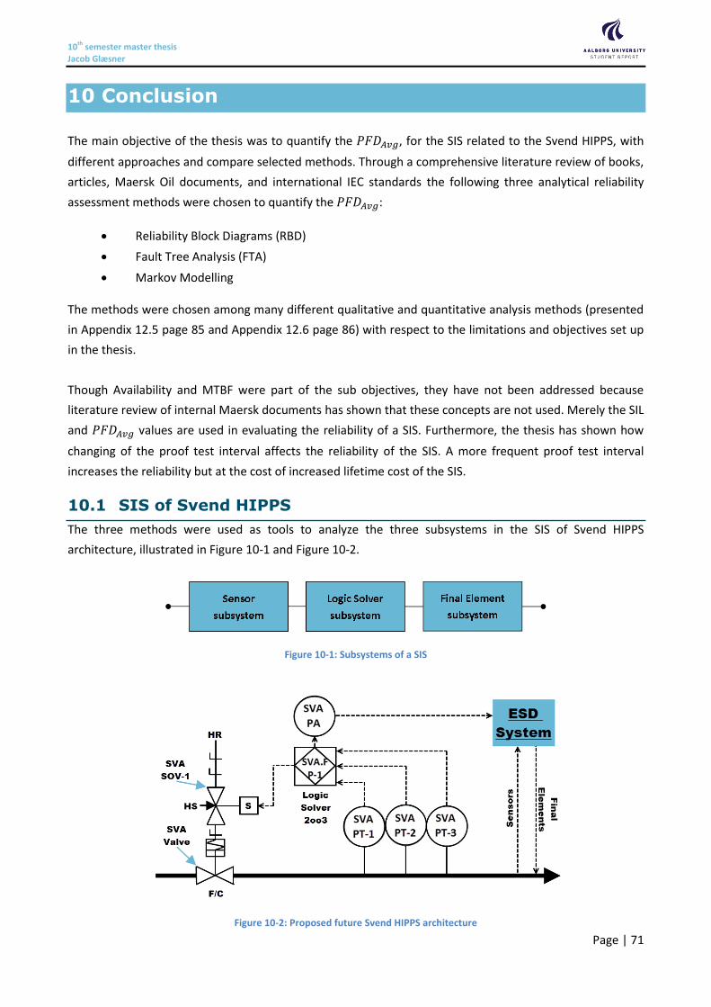
10th semester master thesis Jacob Glæsner
Page | 71
10 Conclusion
The main objective of the thesis was to quantify the 𝑃𝐹𝐷𝐴𝑣𝑔, for the SIS related to the Svend HIPPS, with
different approaches and compare selected methods. Through a comprehensive literature review of books,
articles, Maersk Oil documents, and international IEC standards the following three analytical reliability
assessment methods were chosen to quantify the 𝑃𝐹𝐷𝐴𝑣𝑔:
Reliability Block Diagrams (RBD)
Fault Tree Analysis (FTA)
Markov Modelling
The methods were chosen among many different qualitative and quantitative analysis methods (presented
in Appendix 12.5 page 85 and Appendix 12.6 page 86) with respect to the limitations and objectives set up
in the thesis.
Though Availability and MTBF were part of the sub objectives, they have not been addressed because
literature review of internal Maersk documents has shown that these concepts are not used. Merely the SIL
and 𝑃𝐹𝐷𝐴𝑣𝑔 values are used in evaluating the reliability of a SIS. Furthermore, the thesis has shown how
changing of the proof test interval affects the reliability of the SIS. A more frequent proof test interval
increases the reliability but at the cost of increased lifetime cost of the SIS.
10.1 SIS of Svend HIPPS
The three methods were used as tools to analyze the three subsystems in the SIS of Svend HIPPS
architecture, illustrated in Figure 10-1 and Figure 10-2.
Figure 10-1: Subsystems of a SIS
Figure 10-2: Proposed future Svend HIPPS architecture
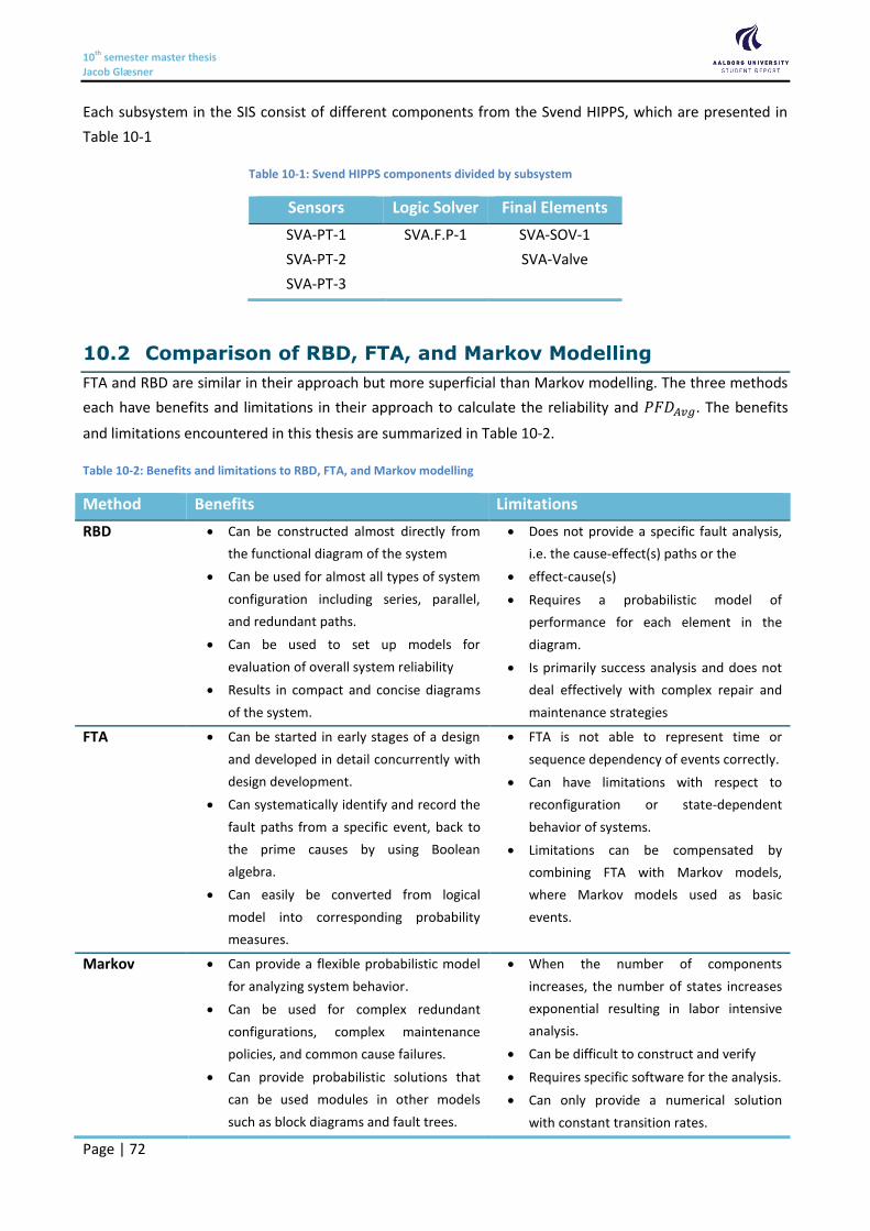
10th semester master thesis Jacob Glæsner
Page | 72
Each subsystem in the SIS consist of different components from the Svend HIPPS, which are presented in
Table 10-1
Table 10-1: Svend HIPPS components divided by subsystem
Sensors Logic Solver Final Elements
SVA-PT-1
SVA-PT-2
SVA-PT-3
SVA.F.P-1 SVA-SOV-1
SVA-Valve
10.2 Comparison of RBD, FTA, and Markov Modelling
FTA and RBD are similar in their approach but more superficial than Markov modelling. The three methods
each have benefits and limitations in their approach to calculate the reliability and 𝑃𝐹𝐷𝐴𝑣𝑔. The benefits
and limitations encountered in this thesis are summarized in Table 10-2.
Table 10-2: Benefits and limitations to RBD, FTA, and Markov modelling
Method Benefits Limitations
RBD Can be constructed almost directly from
the functional diagram of the system
Can be used for almost all types of system
configuration including series, parallel,
and redundant paths.
Can be used to set up models for
evaluation of overall system reliability
Results in compact and concise diagrams
of the system.
Does not provide a specific fault analysis,
i.e. the cause-effect(s) paths or the
effect-cause(s)
Requires a probabilistic model of
performance for each element in the
diagram.
Is primarily success analysis and does not
deal effectively with complex repair and
maintenance strategies
FTA Can be started in early stages of a design
and developed in detail concurrently with
design development.
Can systematically identify and record the
fault paths from a specific event, back to
the prime causes by using Boolean
algebra.
Can easily be converted from logical
model into corresponding probability
measures.
FTA is not able to represent time or
sequence dependency of events correctly.
Can have limitations with respect to
reconfiguration or state-dependent
behavior of systems.
Limitations can be compensated by
combining FTA with Markov models,
where Markov models used as basic
events.
Markov Can provide a flexible probabilistic model
for analyzing system behavior.
Can be used for complex redundant
configurations, complex maintenance
policies, and common cause failures.
Can provide probabilistic solutions that
can be used modules in other models
such as block diagrams and fault trees.
When the number of components
increases, the number of states increases
exponential resulting in labor intensive
analysis.
Can be difficult to construct and verify
Requires specific software for the analysis.
Can only provide a numerical solution
with constant transition rates.
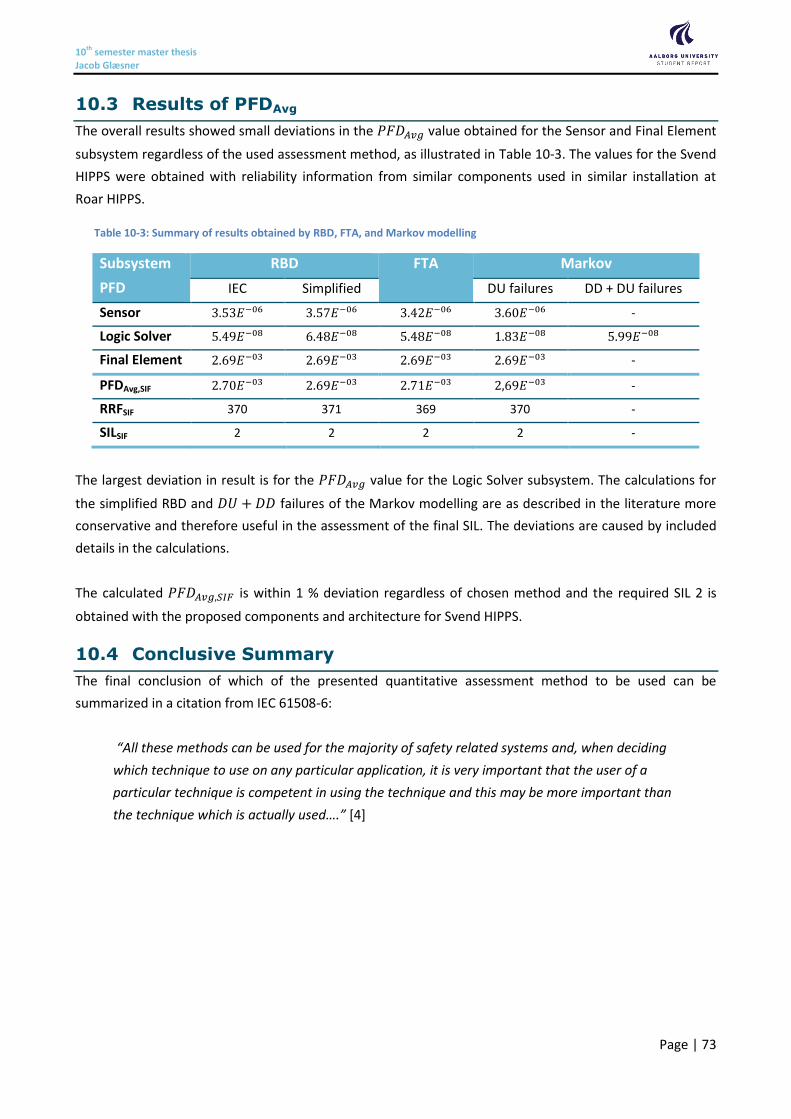
10th semester master thesis Jacob Glæsner
Page | 73
10.3 Results of PFDAvg
The overall results showed small deviations in the 𝑃𝐹𝐷𝐴𝑣𝑔 value obtained for the Sensor and Final Element
subsystem regardless of the used assessment method, as illustrated in Table 10-3. The values for the Svend
HIPPS were obtained with reliability information from similar components used in similar installation at
Roar HIPPS.
Table 10-3: Summary of results obtained by RBD, FTA, and Markov modelling
Subsystem
PFD
RBD FTA Markov
IEC Simplified DU failures DD + DU failures
Sensor 3.53𝐸−06 3.57𝐸−06 3.42𝐸−06 3.60𝐸−06 -
Logic Solver 5.49𝐸−08 6.48𝐸−08 5.48𝐸−08 1.83𝐸−08 5.99𝐸−08
Final Element 2.69𝐸−03 2.69𝐸−03 2.69𝐸−03 2.69𝐸−03 -
PFDAvg,SIF 2.70𝐸−03 2.69𝐸−03 2.71𝐸−03 2,69𝐸−03 -
RRFSIF 370 371 369 370 -
SILSIF 2 2 2 2 -
The largest deviation in result is for the 𝑃𝐹𝐷𝐴𝑣𝑔 value for the Logic Solver subsystem. The calculations for
the simplified RBD and 𝐷𝑈 + 𝐷𝐷 failures of the Markov modelling are as described in the literature more
conservative and therefore useful in the assessment of the final SIL. The deviations are caused by included
details in the calculations.
The calculated 𝑃𝐹𝐷𝐴𝑣𝑔,𝑆𝐼𝐹 is within 1 % deviation regardless of chosen method and the required SIL 2 is
obtained with the proposed components and architecture for Svend HIPPS.
10.4 Conclusive Summary
The final conclusion of which of the presented quantitative assessment method to be used can be
summarized in a citation from IEC 61508-6:
“All these methods can be used for the majority of safety related systems and, when deciding
which technique to use on any particular application, it is very important that the user of a
particular technique is competent in using the technique and this may be more important than
the technique which is actually used….” [4]
10th semester master thesis Jacob Glæsner
Page | 74
11 Bibliography
1. ORS Consulting. LOPA of Svend HIPPS (47.1000.263_R1-A01). s.l. : ORS Consulting, 2016.
2. ISO. ISO/TR 12489:2013 Petroleum, petrochemical and natural gas industries — Reliability modelling and
calculation of safety systems. s.l. : ISO, 2013.
3. Rausand, Marvin. Reliability of Safety-Critical Systems. s.l. : Wiley, 2014. ISBN: 978-1-118-11272-4-
90000.
4. IEC. IEC 61508-6:2010 Functional safety of electrical/electronic/progammable electronic safety-related
systems - Part 6: Guidelines on the application of IEC 61508-2 and IEC 61508-3. s.l. : IEC, 2010.
5. —. IEC 61511-1:2003 Functional safety – Safety instrumented systems for the process industry sector –
Part 1: Framework, definitions, system, hardware and software requirements. s.l. : IEC, 2003.
6. —. IEC 61508-1:2010 Functional safety of electrical/electronic/programmable electronic safety-related
systems – Part 1: General requirements. s.l. : IEC, 2010.
7. Birolini, Alessandro. Reliability Engineering: Theory and Practice. 5th ed. s.l. : Springer, 2007. 978-3-540-
493884.
8. Goble, William M. Control Systems Safety Evaluation and Reliability. s.l. : ISA, 2010. 978-1-934394-80-9.
9. Rausand, Marvin and Høyland, Arnljot. System Reliability Theory: Models, Statistical Methods and
Applications. 2nd ed. s.l. : Wiley, 2004. ISBN: 978-0-471-47133-2.
10. Rausand, Marvin. Risk Assessment: Theory, Methods, and Applications. s.l. : Wiley, 2011. 978-0-470-
63764-7.
11. Zio, Enrico. Series on Quality, Reliability and Engineering Statistics - Vol. 13: An Introduction to the
Basics of Reliability and Risk Analysis. s.l. : World Scientific, 2007. 978-981-270-639-3.
12. —. Series on Quality, Reliability and Engineering Statistics - Vol. 14: Computational Methods for
Reliability and Risk Analysis. s.l. : World Scientific, 2009. 978-981-283-901-5.
13. —. Series on Quality, Reliability and Engineering Statistics - Vol. 15: Basics of Reliability and Risk Analysis
Worked Out Problems and Solutions. s.l. : World Scientific, 2011. 978-981-4355-03-02.
14. OREDA-2009. Offshore Reliability Data Handbook: Volume 1 - Topside Equipment. s.l. : OREDA, 2009.
978-82-14-04830-8.
15. Hauge, Stein. Reliability Data for Safety Instrumented Systems - PDS Data Handbook. s.l. : SINTEF, 2010.

10th semester master thesis Jacob Glæsner
Page | 75
16. A simple reliability block diagram method for safety integrity verification. Guo, Haitao and Yang,
Xianhui. s.l. : Elsevier, October 2nd, 2006, Reliability Engineering and System Safety, Vol. 92, pp. 1267–
1273.
17. Automatic creation of Markov models for reliability assessment of safety instrumented systems. Guo,
Haitao and Yang, Xianhui. s.l. : Elsevier, 2008, Reliability Engineering and System Safety, Vol. 98, pp. 807-
815.
18. Extended block diagram method for a multi-state system reliability assessment. Lisnianski, Anatoly. s.l. :
Elsevier, 2007, Reliability Engineering and System Safety, Vol. 92, pp. 1601-1607.
19. Modeling safety instrumented systems with MooN voting architectures addressing system
reconfiguration for testing. Torres-Echeverría, A.C., Martorell, S. and Thompson, H.A. 2011 : Elsevier,
Reliability Engineering and System Safety, Vol. 96, pp. 545-563.
20. Multi-objective optimization of design and testing of safety instrumented systems with MooN voting
architectures using a genetic algorithm. Torres-Echeverría, A.C., Martorell, S. and Thompson, H.A. s.l. :
Elsevier, 2012, ReliabilityEngineeringandSystemSafety, Vol. 106, pp. 45-60.
21. Modelling and optimization of proof testing policies for safety instrumented systems. Torres-Echeverría,
A.C., Martorell, S. and Thompson, H.A. s.l. : Elsevier, 2009, Reliability Engineering and System Safety, Vol.
94, pp. 838-854.
22. Reliability of safety-instrumented systems subject to partial testing and common-cause failures. Jin, Hui
and Rausand, Marvin. s.l. : Elsevier, 2014, Reliability Engineering and System Safety, Vol. 121, pp. 146-151.
23. Reliability performance of safety instrumented systems: A common approach for both low- and high-
demand mode of operation. Jin, Hui, Lundteigen, Mary Ann and Rausand, Marvin. s.l. : Elsevier, 2011,
Reliability Engineering and System Safety, Vol. 96, pp. 365-373.
24. Hildebrandt, Andreas. Calculating the "Probability of Failure on Demand" (PFD) of complex structures
by means of Markov Models. s.l. : Pepperl+Fuchs GmbH.
25. PFD Calculation Considering Imperfect Proof Tests. Gabriel, Thomas, Hildebrandt, Andreas and Menck,
Udo. [ed.] Eddy de Rademaeker and Peter Schmelzer. s.l. : AIDIC, 2016, CHEMICAL ENGINEERING
TRANSACTIONS, Vol. 48, pp. 637-642.
26. Börcsök, Josef. Comparison of PFD calculation. s.l. : HIMA Paul Hildebrandt GmbH + Co KG.
27. Considering and comparing safety parameters — Using different calculation approaches of
PFD/PFH/HR. Börcsök, Josef and Holub, Petr. s.l. : IEEE, 2011.
28. Calculation of MTTF values with Markov Models for Safety Instrumented Systems. Börcsök, J., Ugljesa,
E. and Machmur, D. [ed.] Department of Computer Architecture and System Programming, University of
Kassel. 2007. 7th WSEAS International Conference on APPLIED COMPUTER SCIENCE, Venice, Italy.
10th semester master thesis Jacob Glæsner
Page | 76
29. Reliability block diagram with general gates and its application to system reliability analysis. Kim, Man
Cheol. s.l. : Elsevier, 2011, Annals of Nuclear Energy, Vol. 38, pp. 2456-2461.
30. NTNU. ROSS Gemini Centre/ Publications/ MSc Theses/ MSc from RAMS group. [Online] [Cited: May
29th, 2017.] https://www.ntnu.edu/ross/msc-theses-rams.
31. IEC. IEC 61508-4:2010 Functional safety of electrical/electronic/programmable electronic safety-related
systems – Part 4: Definitions and abbreviations. s.l. : IEC, 2010.
32. Maersk Oil - website. Maersk > Maersk Oil > Operations. North Sea map. [Online] [Cited: February 21st,
2017.] http://www.maerskoil.com/operations/Pages/operations.aspx.
33. —. Maersk Oil > Operations > Denmark > Oil and gas production. Map of DUC production facilities.
[Online] [Cited: February 21st, 2017.]
http://www.maerskoil.com/operations/Denmark/Documents/DUC%20feltkort_UK_2015_01_mar%20.pdf.
34. Maersk Oil - document control. SVAY-14-00042-0001 - rev. 1, Isometric Views. s.l. : Maersk Oil,
February 7th, 2012.
35. IEC. IEC 61511-3:2003 Functional safety – Safety instrumented systems for the process industry sector –
Part 3: Guidance for the determination of the required safety integrity levels. s.l. : IEC, 2003.
36. Maersk Oil - document control. Standard - MOTS-46 High Integrity Protection System (MOG-FP-SAF-
STD-0046 Rev. 2.0). s.l. : MAersk, September 1st, 2016.
37. —. Standard - Safety Integrity Level (SIL) Analysis (MOG-FP-SAF-STD-0102 Rev 1.0). s.l. : Maersk Oil,
January 3rd, 2014.
38. Fleming, K. N. A reliability model for common cause mode failures in redundant safety systems,
Technical Report GA-A13284. San Diego, Ca. : General Atomic Company, 1975.
39. Hauge, Stein, et al., et al. Reliability Prediction Method for Safety Instrumented Systems: PDS Method
Handbook 2013 Edition. s.l. : SINTEF, 2013. 978-82-536-1333-8.
40. IEC. IEC 61078:2016 Reliability block diagrams. s.l. : IEC, 2016.
41. —. IEC 61025:2006 Fault Tree Analysis (FTA). s.l. : IEC, 2006.
42. Glæsner, Jacob. Case-based report: Maersk Oil Svend Platform HIPPS Upgrade. s.l. : Jacob Glæsner,
2017.
43. Maersk Oil - document control. SVAY-04-00014-0002 - rev. 11, SVA P&ID export riser. s.l. : Maersk Oil,
June 14th, 2016.
44. —. Svend General Documentation. s.l. : Maersk Oil, June 2012.
45. ITOPF. Fate of Marine Oil Spills - Technical Information Paper. London : ITOPF, 2011.
10th semester master thesis Jacob Glæsner
Page | 77
46. Maersk Oil - document control. DBU Oil Spill Risk Assessment (DK-HSE-PRD-0001 Rev 1.0). s.l. : Maersk
Oil, April 26th, 2015.
47. IEC. IEC 61508-7:2010 Functional safety of electrical/electronic/programmable electronic safety-related
systems – Part 7: Overview of techniques and measures. s.l. : IEC, 2010.
48. —. IEC 60300-3-1:2003 Dependability management – Part 3-1: Application guide – Analysis techniques
for dependability – Guide on methodology. 2003.
49. Maersk Oil - document control. SVAY-03-00023-0000 - rev. 3, SVA HIPPS Schematic export pipeline.
s.l. : Maersk Oil, September 8th, 2015.
50. Wakerly, John F. Digital Design: Principles and Practices. 4th. s.l. : Pearson, 2006. pp. 179-234. ISBN:
978-81-317-1366-2.
51. IEC. IEC 60300-3-2:2004 Dependability management – Part 3-2: Application guide – Collection of
dependability data from the field. s.l. : IEC, 2004.
52. —. IEC 60300-3-4:2007 Dependability management – Part 3-4: Application guide – Guide to the
specification of dependability requirements. s.l. : IEC, 2007.
53. —. IEC 60812:2006 Analysis techniques for system reliability – Procedure for failure mode and effects
analysis (FMEA). s.l. : IEC, 2006.
54. —. IEC 61508-2:2010 Functional safety of electrical/electronic/programmable electronic safety-related
systems – Part 2: Requirements for electrical/electronic/programmable electronic safety-related systems.
s.l. : IEC, 2010.
55. —. IEC 61508-3:2010 Functional safety of electrical/electronic/programmable electronic safety-related
systems – Part 3: Software requirements. s.l. : IEC, 2010.
56. —. IEC 61508-5:2010 Functional safety of electrical/electronic/programmable electronic safety-related
systems – Part 5: Examples of methods for the determination of safety integrity levels. s.l. : IEC, 2010.
57. —. IEC 61511-2:2003 Functional safety – Safety instrumented systems for the process industry sector –
Part 2: Guidelines for the application of IEC 61511-1. s.l. : IEC, 2003.
58. —. IEC 62551:2012 Analysis techniques for dependability – Petri net techniques. s.l. : IEC, 2012.
59. —. IEC 60050-351:2013 International electrotechnical vocabulary – Part 351: Control technology. s.l. :
IEC, 2013.
60. —. IEC 60050-151:2001 International Electrotechnical Vocabulary – Part 151: Electrical and magnetic
devices. s.l. : IEC, 2001.
10th semester master thesis Jacob Glæsner
Page | 78
61. —. IEC/TR 62380:2004 Reliability data handbook – Universal model for reliability prediction of
electronics components, PCBs and equipment. s.l. : IEC, 2004.
62. ISO. ISO 10418:2003 Petroleum and natural gas industries — Offshore production installations — Basic
surface process safety systems. s.l. : ISO, 2003.
63. —. ISO 13702:2015 Petroleum and natural gas industries — Control and mitigation of fires and
explosions on offshore production installations — Requirements and guidelines. s.l. : ISO, 2015.
64. —. ISO 14224:2016 Petroleum, petrochemical and natural gas industries — Collection and exchange of
reliability and maintenance data for equipment. s.l. : ISO, 2016.
65. —. ISO 17776:2000 Petroleum and natural gas industries — Offshore production installations —
Guidelines on tools and techniques for hazard identification and risk assessment. s.l. : ISO, 2000.
66. IEC. IEC 61703:2016 Mathematical expressions for reliability, availability, maintainability and
maintenance support terms. s.l. : IEC, 2016.
67. —. IEC 61165:2006 Application of Markov techniques. s.l. : IEC, 2006.
68. Limnios, Nikolaos. Fault Trees. s.l. : ISTE, 2007. ISBN: 978-1-905209-30-9.

10th semester master thesis Jacob Glæsner
Page | 79
12 Appendix
(This page is intentionally left blank)
10th semester master thesis Jacob Glæsner
Page | 80
12.1 Hazard Scenarios [42]
Eight hazard scenarios were identified prior to the LOPA study and merged into following five initiating
causes:
a) Stuck pig
A blockage due to a stuck pig occurs in the sub-sea tee piece downstream the Svend riser or further
downstream in the export pipeline to Tyra East. Pigging facilities are present on Svend, however
pigging might be difficult as the pig historically has been difficult to drive to Tyra East due to the
sub-sea tee piece. Notice that there is a check valve installed in the riser prior to entering the sub-
see tee piece according to the P&ID SVAY-04-00014-0002 rev 11 [43]. Pigging occurs regularly from
Harald to Tyra East (approx. once per month).
b) Hydrate formation
A blockage due to hydrate formation occurs just downstream the hose on Svend riser or further
downstream in the export pipeline to Tyra East. Hydrate formation is unlikely in normal situations
as well fluid is relatively warm from Svend. However well fluid coolers are installed and could cool
down to hydrate formation temperature if control does not work properly [44].
c) Wax plug
A blockage due to a wax plug occurs downstream the hose or in the pipeline downstream the sub-
sea tee-piece since Lulita, Trym and Svend fluid is waxy [44].
d) Closed Tyra East inlet
Path into Tyra East gets closed, while Svend is still producing to the pipeline. This could be due to
riser ESDV closure (ESDV-18010) or inlet ESDV closure (ESDV-18101).
e) Stuck check valve
Stuck check valve downstream flexible hose.
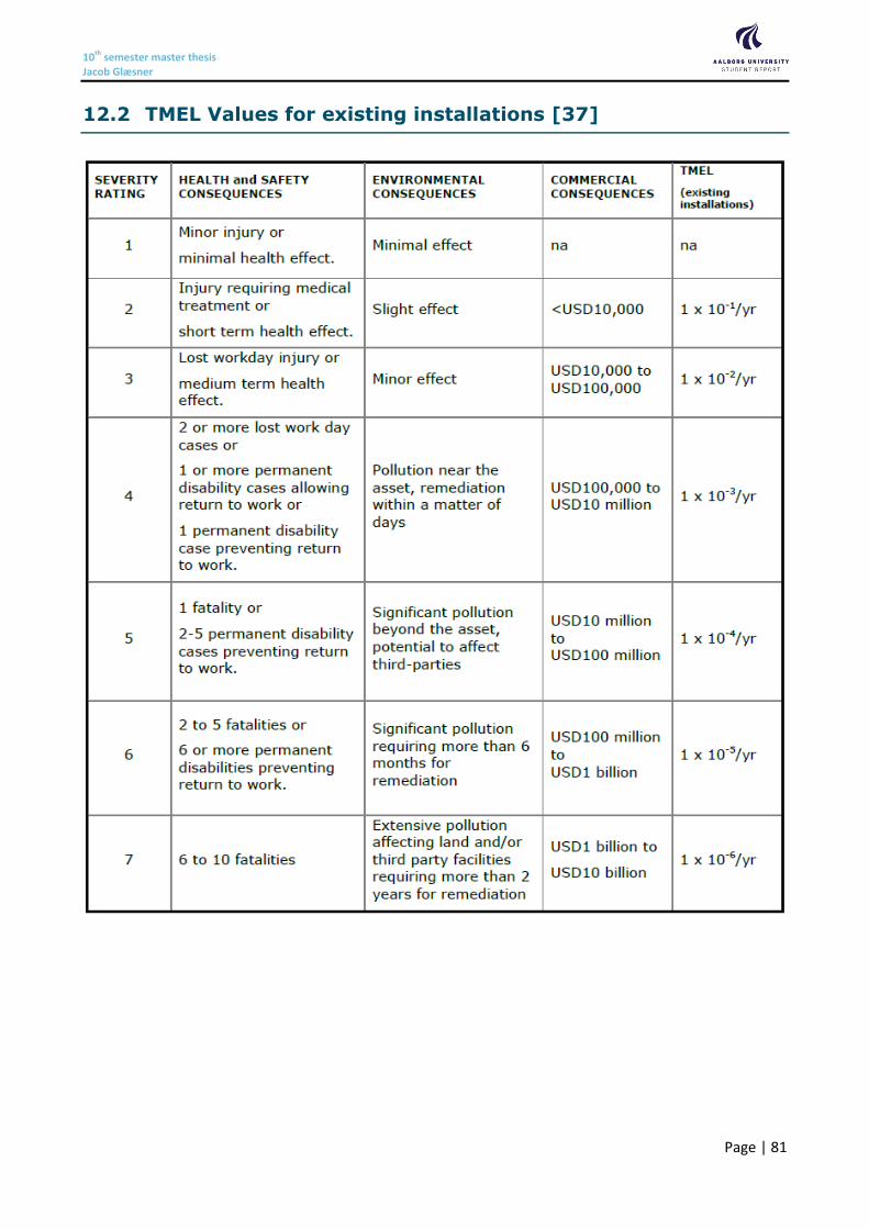
10th semester master thesis Jacob Glæsner
Page | 81
12.2 TMEL Values for existing installations [37]

10th semester master thesis Jacob Glæsner
Page | 82
12.3 Oil Group Classification [45] [46]
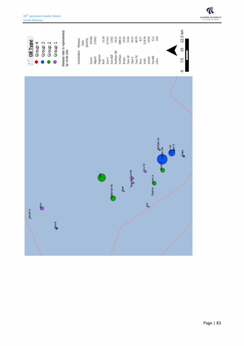
10th semester master thesis Jacob Glæsner
Page | 83
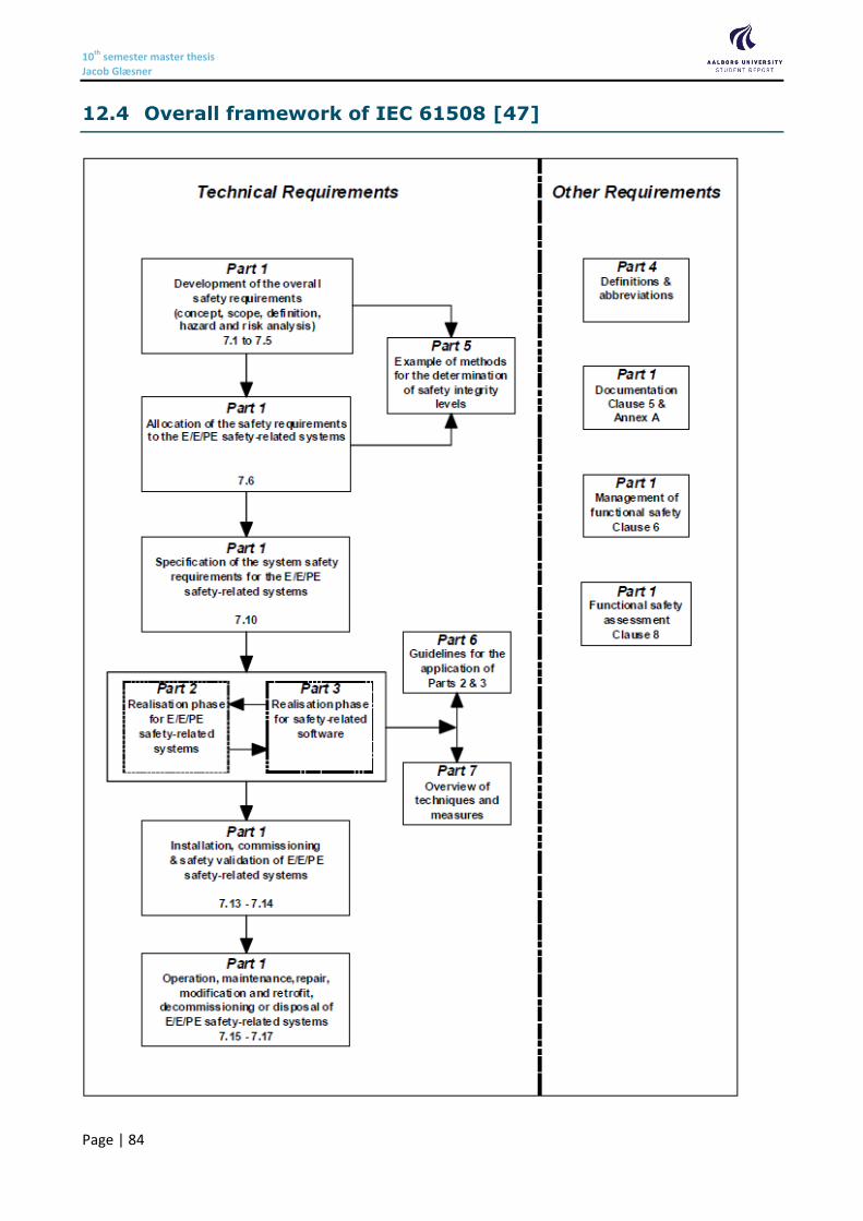
10th semester master thesis Jacob Glæsner
Page | 84
12.4 Overall framework of IEC 61508 [47]
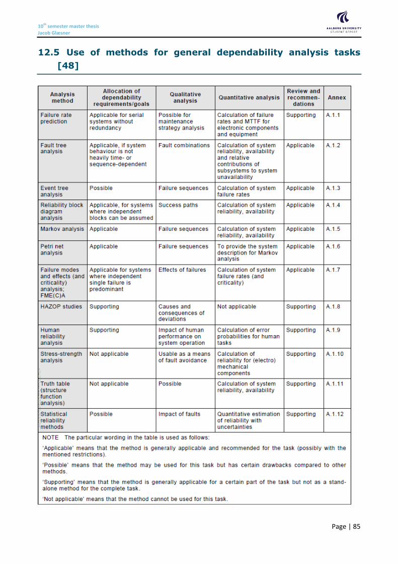
10th semester master thesis Jacob Glæsner
Page | 85
12.5 Use of methods for general dependability analysis tasks
[48]
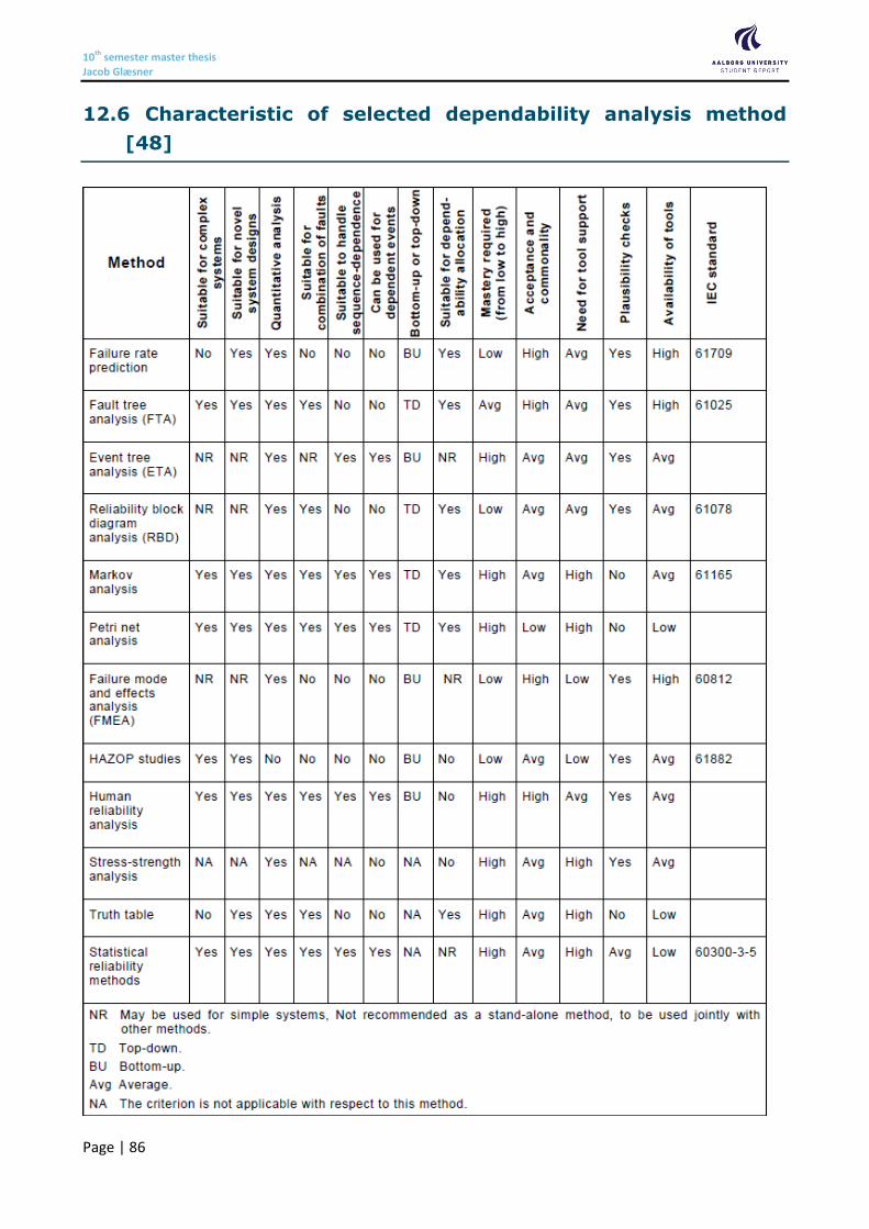
10th semester master thesis Jacob Glæsner
Page | 86
12.6 Characteristic of selected dependability analysis method
[48]
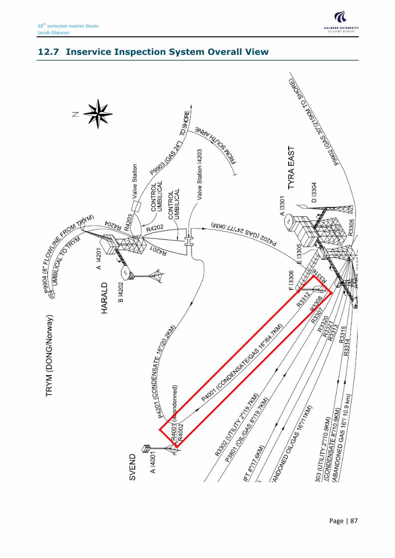
10th semester master thesis Jacob Glæsner
Page | 87
12.7 Inservice Inspection System Overall View
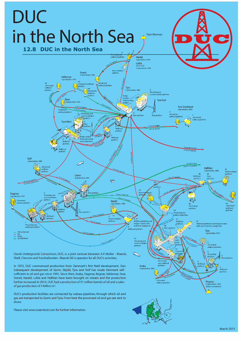
10th semester master thesis Jacob Glæsner
Page | 88
12.8 DUC in the North Sea
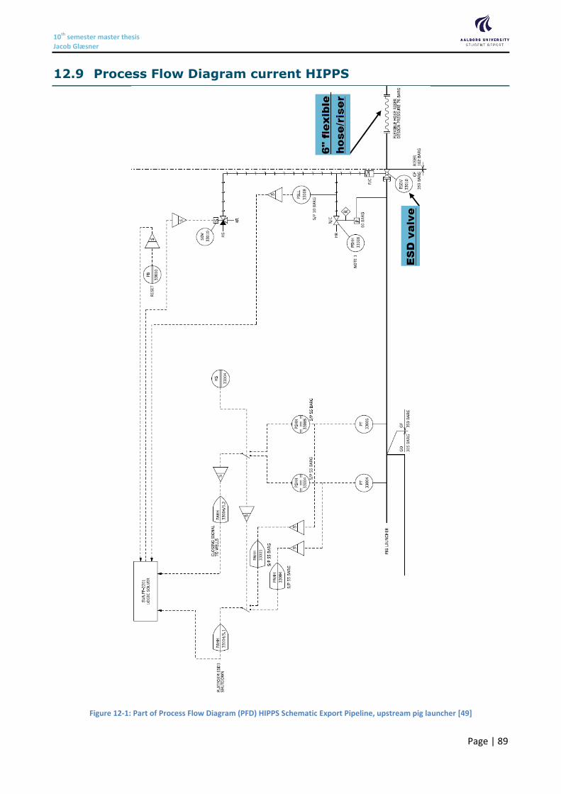
10th semester master thesis Jacob Glæsner
Page | 89
12.9 Process Flow Diagram current HIPPS
Figure 12-1: Part of Process Flow Diagram (PFD) HIPPS Schematic Export Pipeline, upstream pig launcher [49]
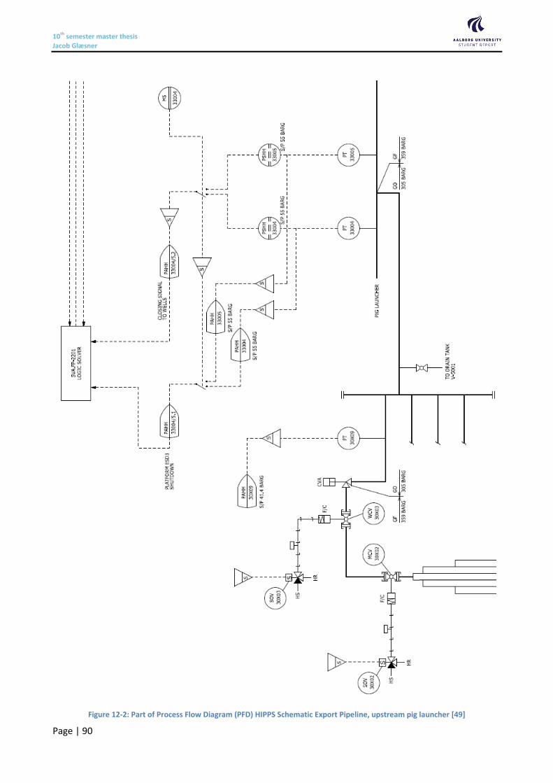
10th semester master thesis Jacob Glæsner
Page | 90
Figure 12-2: Part of Process Flow Diagram (PFD) HIPPS Schematic Export Pipeline, upstream pig launcher [49]
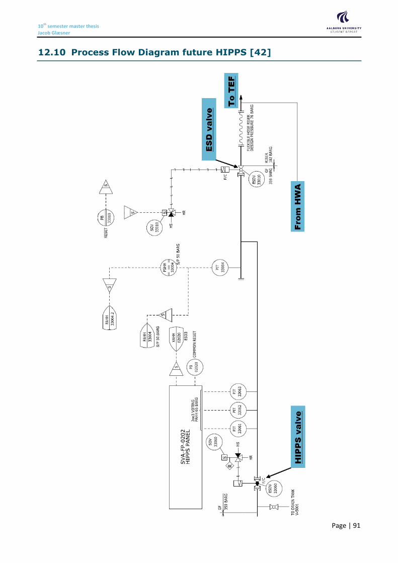
10th semester master thesis Jacob Glæsner
Page | 91
12.10 Process Flow Diagram future HIPPS [42]
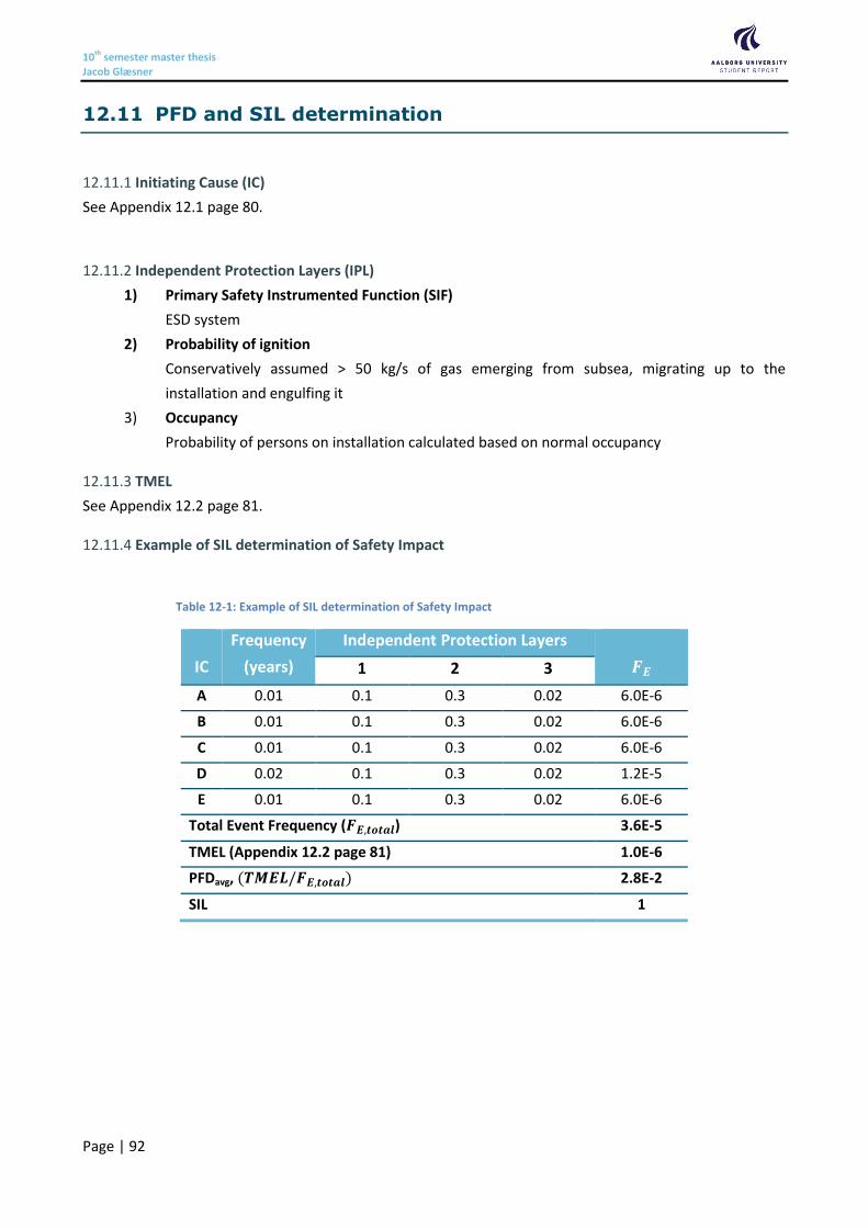
10th semester master thesis Jacob Glæsner
Page | 92
12.11 PFD and SIL determination
Initiating Cause (IC) 12.11.1
See Appendix 12.1 page 80.
Independent Protection Layers (IPL) 12.11.2
1) Primary Safety Instrumented Function (SIF)
ESD system
2) Probability of ignition
Conservatively assumed > 50 kg/s of gas emerging from subsea, migrating up to the
installation and engulfing it
3) Occupancy
Probability of persons on installation calculated based on normal occupancy
TMEL 12.11.3
See Appendix 12.2 page 81.
Example of SIL determination of Safety Impact 12.11.4
Table 12-1: Example of SIL determination of Safety Impact
IC
Frequency
(years)
Independent Protection Layers
𝑭𝑬 1 2 3
A 0.01 0.1 0.3 0.02 6.0E-6
B 0.01 0.1 0.3 0.02 6.0E-6
C 0.01 0.1 0.3 0.02 6.0E-6
D 0.02 0.1 0.3 0.02 1.2E-5
E 0.01 0.1 0.3 0.02 6.0E-6
Total Event Frequency (𝑭𝑬,𝒕𝒐𝒕𝒂𝒍) 3.6E-5
TMEL (Appendix 12.2 page 81) 1.0E-6
PFDavg, (𝑻𝑴𝑬𝑳/𝑭𝑬,𝒕𝒐𝒕𝒂𝒍) 2.8E-2
SIL 1

10th semester master thesis Jacob Glæsner
Page | 93
12.12 2oo3 Structure Function
Minimal Path Set 12.12.1
The structure function for 2oo3 voting as represented in Eq. 6-10 page 36 is derived using a combination of
series and parallel structures and the Minimal Path Sets, which is the minimal path through the system that
still secures the system in up state. The different paths are illustrated in Figure 12-3.
Figure 12-3: Minimal Path Set of a 2oo3 RBD
The approach is similar for other moon structures.
ϕ(𝑿) = 𝑥1 ∩ 𝑥2 ∪ 𝑥1 ∩ 𝑥3 ∪ 𝑥2 ∩ 𝑥3
= 𝑥1𝑥2 ∪ 𝑥1𝑥3 ∪ 𝑥2𝑥3
= 1 − (1 − 𝑥1𝑥2)(1 − 𝑥1𝑥3)(1 − 𝑥2𝑥3)
= 1 − (1 − 𝑥1𝑥2 − 𝑥1𝑥3 + 𝑥12𝑥2𝑥3)(1 − 𝑥2𝑥3)
= 1 − (1 − 𝑥1𝑥2 − 𝑥1𝑥3 + 𝑥12𝑥2𝑥3 − 𝑥2𝑥3 + 𝑥1𝑥2
2𝑥3 + 𝑥1𝑥2𝑥32 − 𝑥1
2𝑥22𝑥3
2)
= 𝑥1𝑥2 + 𝑥1𝑥3 + 𝑥2𝑥3 − 𝑥12𝑥2𝑥3 − 𝑥1𝑥2
2𝑥3 − 𝑥1𝑥2𝑥32 + 𝑥1
2𝑥22𝑥3
2
𝑥𝑖 is binary so 𝑥𝑖𝑚 = 𝑥𝑖
= 𝑥1𝑥2 + 𝑥1𝑥3 + 𝑥2𝑥3 − 𝑥1𝑥2𝑥3 − 𝑥1𝑥2𝑥3 − 𝑥1𝑥2𝑥3 + 𝑥1𝑥2𝑥3
= 𝑥1𝑥2 + 𝑥1𝑥3 + 𝑥2𝑥3 − 2𝑥1𝑥2𝑥3 = Eq. 6-10 page 36
Minimal Cut Set 12.12.2
Another approach to derive Eq. 6-10 page 36 is by following a Minimal Cut Set. A cut set is a set of
components that by failing puts the system in down state. The RBD of this is illustrated in Figure 12-4.
Figure 12-4: Minimal Cut Set of a 2oo3 RBD

10th semester master thesis Jacob Glæsner
Page | 94
The approach is similar for other moon structures.
ϕ(𝑿) = 𝑥1 ∪ 𝑥2 ∩ 𝑥1 ∪ 𝑥3 ∩ 𝑥2 ∪ 𝑥3
= (𝑥1 ∪ 𝑥2)(𝑥1 ∪ 𝑥3)(𝑥2 ∪ 𝑥3)
= (1 − (1 − 𝑥1)(1 − 𝑥2))(1 − (1 − 𝑥1)(1 − 𝑥3))(1 − (1 − 𝑥2)(1 − 𝑥3))
= (𝑥1 + 𝑥2 − 𝑥1𝑥2)(𝑥1 + 𝑥3 − 𝑥1𝑥3)(𝑥2 + 𝑥3 − 𝑥2𝑥3)
= (𝑥12 + 𝑥1𝑥3 − 𝑥1
2𝑥3 + 𝑥1𝑥2 + 𝑥2𝑥3 − 𝑥1𝑥2𝑥3 − 𝑥12𝑥2 − 𝑥1𝑥2𝑥3 + 𝑥1
2𝑥2𝑥3)(𝑥2
+ 𝑥3 − 𝑥2𝑥3)
𝑥𝑖 is binary so 𝑥𝑖𝑚 = 𝑥𝑖
= (𝑥1 + 𝑥2𝑥3 − 𝑥1𝑥2𝑥3)(𝑥2 + 𝑥3 − 𝑥2𝑥3)
= 𝑥1𝑥2 + 𝑥1𝑥3 − 𝑥1𝑥2𝑥3 + 𝑥22𝑥3 + 𝑥2𝑥3
2 − 𝑥22𝑥3
2 − 𝑥1𝑥22𝑥3 − 𝑥1𝑥2𝑥3
2 + 𝑥1𝑥22𝑥3
2
𝑥𝑖 is binary so 𝑥𝑖𝑚 = 𝑥𝑖
= 𝑥1𝑥2 + 𝑥1𝑥3 + 𝑥2𝑥3 − 2𝑥1𝑥2𝑥3
= Eq. 6-10 page 36
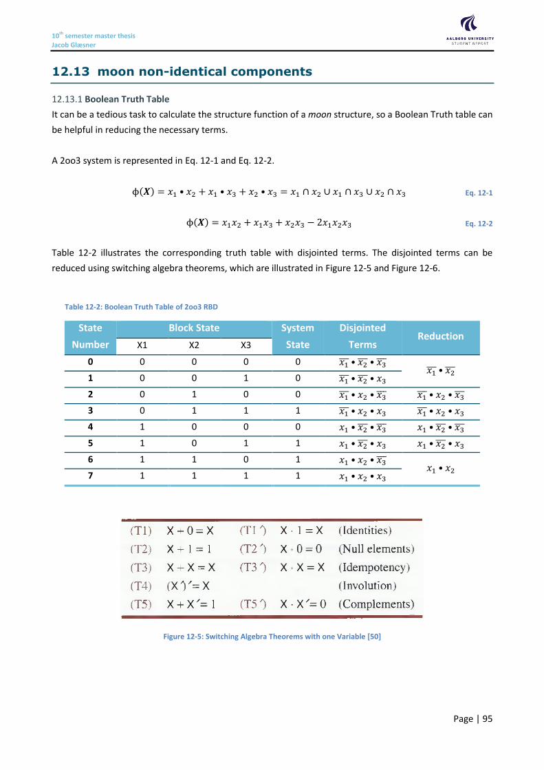
10th semester master thesis Jacob Glæsner
Page | 95
12.13 moon non-identical components
Boolean Truth Table 12.13.1
It can be a tedious task to calculate the structure function of a moon structure, so a Boolean Truth table can
be helpful in reducing the necessary terms.
A 2oo3 system is represented in Eq. 12-1 and Eq. 12-2.
ϕ(𝑿) = 𝑥1 • 𝑥2 + 𝑥1 • 𝑥3 + 𝑥2 • 𝑥3 = 𝑥1 ∩ 𝑥2 ∪ 𝑥1 ∩ 𝑥3 ∪ 𝑥2 ∩ 𝑥3 Eq. 12-1
ϕ(𝑿) = 𝑥1𝑥2 + 𝑥1𝑥3 + 𝑥2𝑥3 − 2𝑥1𝑥2𝑥3 Eq. 12-2
Table 12-2 illustrates the corresponding truth table with disjointed terms. The disjointed terms can be
reduced using switching algebra theorems, which are illustrated in Figure 12-5 and Figure 12-6.
Table 12-2: Boolean Truth Table of 2oo3 RBD
State
Number
Block State System
State
Disjointed
Terms Reduction
X1 X2 X3
0 0 0 0 0 𝑥1̅̅ ̅ • 𝑥2̅̅ ̅ • 𝑥3̅̅ ̅ 𝑥1̅̅ ̅ • 𝑥2̅̅ ̅
1 0 0 1 0 𝑥1̅̅ ̅ • 𝑥2̅̅ ̅ • 𝑥3
2 0 1 0 0 𝑥1̅̅ ̅ • 𝑥2 • 𝑥3̅̅ ̅ 𝑥1̅̅ ̅ • 𝑥2 • 𝑥3̅̅ ̅
3 0 1 1 1 𝑥1̅̅ ̅ • 𝑥2 • 𝑥3 𝑥1̅̅ ̅ • 𝑥2 • 𝑥3
4 1 0 0 0 𝑥1 • 𝑥2̅̅ ̅ • 𝑥3̅̅ ̅ 𝑥1 • 𝑥2̅̅ ̅ • 𝑥3̅̅ ̅
5 1 0 1 1 𝑥1 • 𝑥2̅̅ ̅ • 𝑥3 𝑥1 • 𝑥2̅̅ ̅ • 𝑥3
6 1 1 0 1 𝑥1 • 𝑥2 • 𝑥3̅̅ ̅ 𝑥1 • 𝑥2
7 1 1 1 1 𝑥1 • 𝑥2 • 𝑥3
Figure 12-5: Switching Algebra Theorems with one Variable [50]
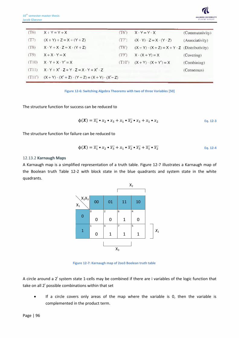
10th semester master thesis Jacob Glæsner
Page | 96
Figure 12-6: Switching Algebra Theorems with two of three Variables [50]
The structure function for success can be reduced to
ϕ(𝑿) = 𝑥1̅̅ ̅ • 𝑥2 • 𝑥3 + 𝑥1 • 𝑥2̅̅ ̅ • 𝑥3 + 𝑥1 • 𝑥2 Eq. 12-3
The structure function for failure can be reduced to
ϕ(𝑿) = 𝑥1̅̅ ̅ • 𝑥2 • 𝑥3̅̅ ̅ + 𝑥1 • 𝑥2̅̅ ̅ • 𝑥3̅̅ ̅ + 𝑥1̅̅ ̅ • 𝑥2̅̅ ̅ Eq. 12-4
Karnaugh Maps 12.13.2
A Karnaugh map is a simplified representation of a truth table. Figure 12-7 illustrates a Karnaugh map of
the Boolean truth Table 12-2 with block state in the blue quadrants and system state in the white
quadrants.
A circle around a 2i system state 1-cells may be combined if there are i variables of the logic function that
take on all 2i possible combinations within that set
If a circle covers only areas of the map where the variable is 0, then the variable is
complemented in the product term.
X2
X2X3
X1 00 01 11 10
0 0 2 6 4
0 0 1 0
1 1 3 7 5
X1 0 1 1 1
X3
Figure 12-7: Karnaugh map of 2oo3 Boolean truth table
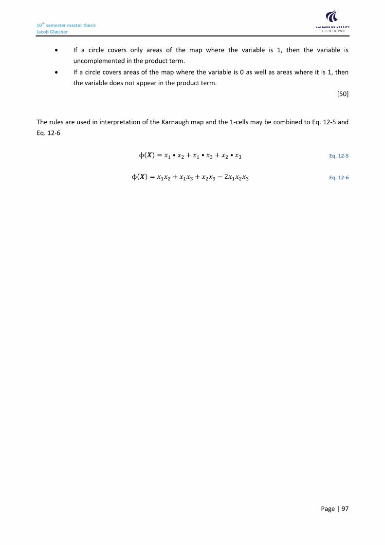
10th semester master thesis Jacob Glæsner
Page | 97
If a circle covers only areas of the map where the variable is 1, then the variable is
uncomplemented in the product term.
If a circle covers areas of the map where the variable is 0 as well as areas where it is 1, then
the variable does not appear in the product term.
[50]
The rules are used in interpretation of the Karnaugh map and the 1-cells may be combined to Eq. 12-5 and
Eq. 12-6
ϕ(𝑿) = 𝑥1 • 𝑥2 + 𝑥1 • 𝑥3 + 𝑥2 • 𝑥3 Eq. 12-5
ϕ(𝑿) = 𝑥1𝑥2 + 𝑥1𝑥3 + 𝑥2𝑥3 − 2𝑥1𝑥2𝑥3 Eq. 12-6
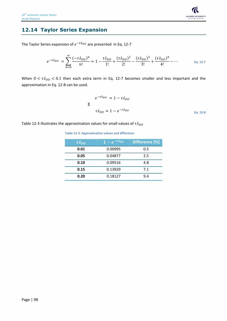
10th semester master thesis Jacob Glæsner
Page | 98
12.14 Taylor Series Expansion
The Taylor Series expansion of 𝑒−𝜏𝜆𝐷𝑈 are presented in Eq. 12-7
𝑒−𝜏𝜆𝐷𝑈 = ∑(−𝜏𝜆𝐷𝑈)𝑛
𝑛!
∞
𝑛=0
= 1 −𝜏𝜆𝐷𝑈
1!+
(𝜏𝜆𝐷𝑈)2
2!−
(𝜏𝜆𝐷𝑈)3
3!+
(𝜏𝜆𝐷𝑈)4
4!− ⋯ Eq. 12-7
When 0 < 𝜏𝜆𝐷𝑈 < 0.1 then each extra term in Eq. 12-7 becomes smaller and less important and the
approximation in Eq. 12-8 can be used.
𝑒−𝜏𝜆𝐷𝑈 ≈ 1 − 𝜏𝜆𝐷𝑈
Eq. 12-8
⇕
𝜏𝜆𝐷𝑈 ≈ 1 − 𝑒−𝜏𝜆𝐷𝑈
Table 12-3 illustrates the approximation values for small values of 𝜏𝜆𝐷𝑈
Table 12-3: Approximation values and difference
𝝉𝝀𝑫𝑼 𝟏 − 𝒆−𝝉𝝀𝑫𝑼 Difference [%]
0.01 0.00995 0.5
0.05 0.04877 2.5
0.10 0.09516 4.8
0.15 0.13929 7.1
0.20 0.18127 9.4
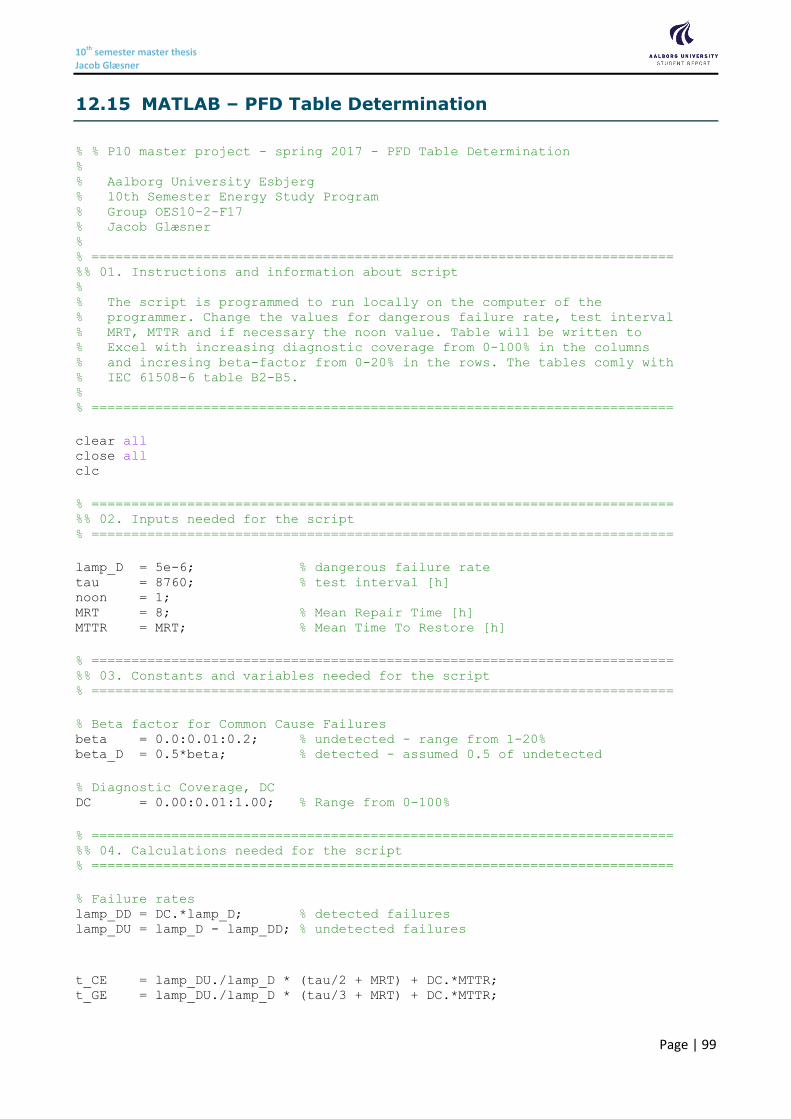
10th semester master thesis Jacob Glæsner
Page | 99
12.15 MATLAB – PFD Table Determination
% % P10 master project - spring 2017 - PFD Table Determination % % Aalborg University Esbjerg % 10th Semester Energy Study Program % Group OES10-2-F17 % Jacob Glæsner % % ========================================================================= %% 01. Instructions and information about script % % The script is programmed to run locally on the computer of the % programmer. Change the values for dangerous failure rate, test interval % MRT, MTTR and if necessary the noon value. Table will be written to % Excel with increasing diagnostic coverage from 0-100% in the columns % and incresing beta-factor from 0-20% in the rows. The tables comly with % IEC 61508-6 table B2-B5. % % =========================================================================
clear all close all clc
% ========================================================================= %% 02. Inputs needed for the script % =========================================================================
lamp_D = 5e-6; % dangerous failure rate tau = 8760; % test interval [h] noon = 1; MRT = 8; % Mean Repair Time [h] MTTR = MRT; % Mean Time To Restore [h]
% ========================================================================= %% 03. Constants and variables needed for the script % =========================================================================
% Beta factor for Common Cause Failures beta = 0.0:0.01:0.2; % undetected - range from 1-20% beta_D = 0.5*beta; % detected - assumed 0.5 of undetected
% Diagnostic Coverage, DC DC = 0.00:0.01:1.00; % Range from 0-100%
% ========================================================================= %% 04. Calculations needed for the script % =========================================================================
% Failure rates lamp_DD = DC.*lamp_D; % detected failures lamp_DU = lamp_D - lamp_DD; % undetected failures
t_CE = lamp_DU./lamp_D * (tau/2 + MRT) + DC.*MTTR; t_GE = lamp_DU./lamp_D * (tau/3 + MRT) + DC.*MTTR;
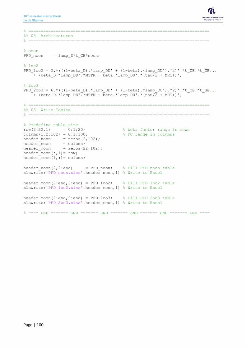
10th semester master thesis Jacob Glæsner
Page | 100
% ========================================================================= %% 05. Architectures % =========================================================================
% noon PFD_noon = lamp_D*t_CE*noon;
% 1oo2 PFD_1oo2 = 2.*(((1-beta_D).*lamp_DD' + (1-beta).*lamp_DU').^2)'.*t_CE.*t_GE... + (beta_D.*lamp_DD'.*MTTR + beta.*lamp_DU'.*(tau/2 + MRT))';
% 2oo3 PFD_2oo3 = 6.*(((1-beta_D).*lamp_DD' + (1-beta).*lamp_DU').^2)'.*t_CE.*t_GE... + (beta_D.*lamp_DD'.*MTTR + beta.*lamp_DU'.*(tau/2 + MRT))';
% ========================================================================= %% 06. Write Tables % =========================================================================
% Predefine table size row(2:22,1) = 0:1:20; % beta factor range in rows column(1,2:102) = 0:1:100; % DC range in columns header_noon = zeros(2,102); header_noon = column; header_moon = zeros(22,102); header_moon(:,1)= row; header_moon(1,:)= column;
header_noon(2,2:end) = PFD_noon; % Fill PFD_noon table xlswrite('PFD_noon.xlsx',header_noon,1) % Write to Excel
header_moon(2:end,2:end) = PFD_1oo2; % Fill PFD_1oo2 table xlswrite('PFD_1oo2.xlsx',header_moon,1) % Write to Excel
header_moon(2:end,2:end) = PFD_2oo3; % Fill PFD_2oo3 table xlswrite('PFD_2oo3.xlsx',header_moon,1) % Write to Excel
% ==== END ======= END ======= END ======= END ======= END ======= END ====
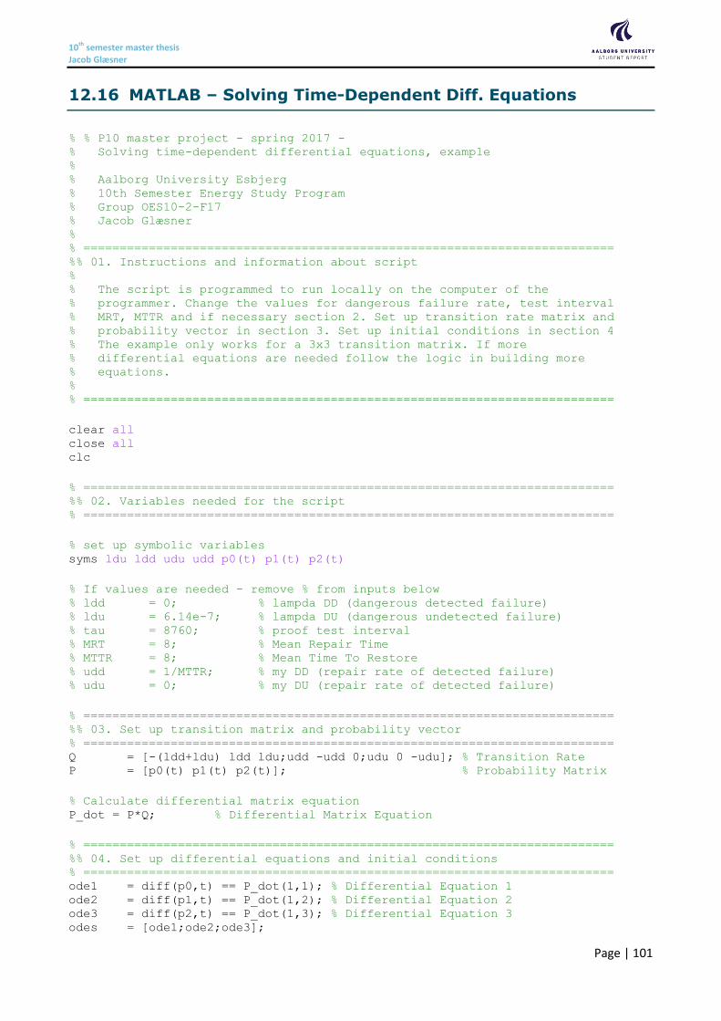
10th semester master thesis Jacob Glæsner
Page | 101
12.16 MATLAB – Solving Time-Dependent Diff. Equations
% % P10 master project - spring 2017 - % Solving time-dependent differential equations, example % % Aalborg University Esbjerg % 10th Semester Energy Study Program % Group OES10-2-F17 % Jacob Glæsner % % ========================================================================= %% 01. Instructions and information about script % % The script is programmed to run locally on the computer of the % programmer. Change the values for dangerous failure rate, test interval % MRT, MTTR and if necessary section 2. Set up transition rate matrix and % probability vector in section 3. Set up initial conditions in section 4 % The example only works for a 3x3 transition matrix. If more % differential equations are needed follow the logic in building more % equations. % % =========================================================================
clear all close all clc
% ========================================================================= %% 02. Variables needed for the script % =========================================================================
% set up symbolic variables syms ldu ldd udu udd p0(t) p1(t) p2(t)
% If values are needed - remove % from inputs below % ldd = 0; % lampda DD (dangerous detected failure) % ldu = 6.14e-7; % lampda DU (dangerous undetected failure) % tau = 8760; % proof test interval % MRT = 8; % Mean Repair Time % MTTR = 8; % Mean Time To Restore % udd = 1/MTTR; % my DD (repair rate of detected failure) % udu = 0; % my DU (repair rate of detected failure)
% ========================================================================= %% 03. Set up transition matrix and probability vector % ========================================================================= Q = [-(ldd+ldu) ldd ldu;udd -udd 0;udu 0 -udu]; % Transition Rate P = [p0(t) p1(t) p2(t)]; % Probability Matrix
% Calculate differential matrix equation P_dot = P*Q; % Differential Matrix Equation
% ========================================================================= %% 04. Set up differential equations and initial conditions % ========================================================================= ode1 = diff(p0,t) == P_dot(1,1); % Differential Equation 1 ode2 = diff(p1,t) == P_dot(1,2); % Differential Equation 2 ode3 = diff(p2,t) == P_dot(1,3); % Differential Equation 3 odes = [ode1;ode2;ode3];
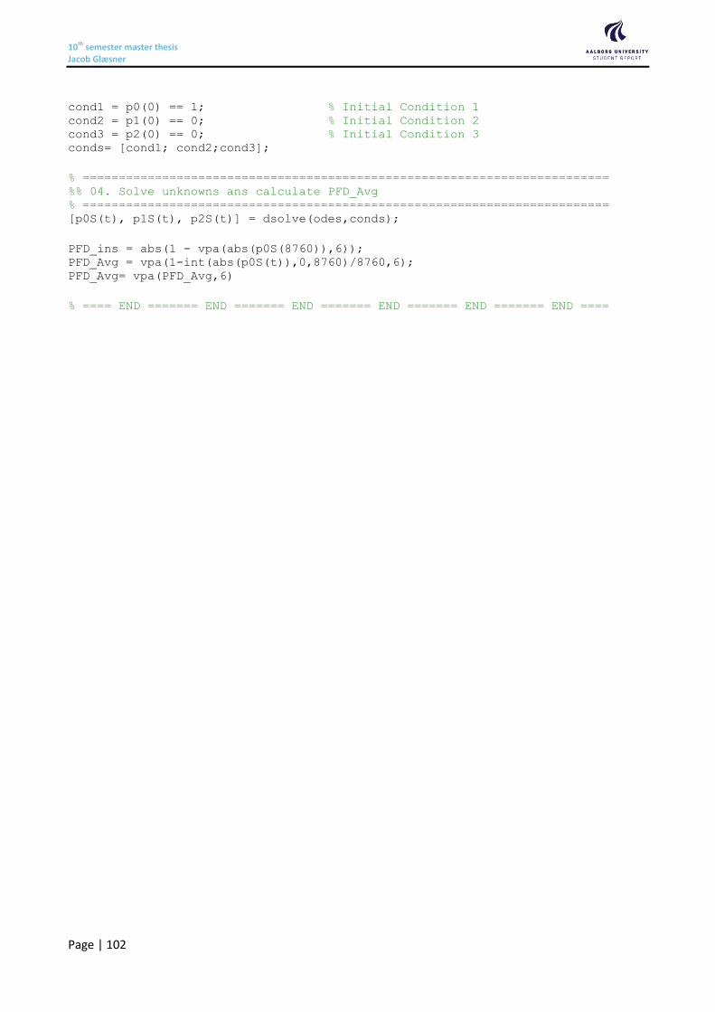
10th semester master thesis Jacob Glæsner
Page | 102
cond1 = p0(0) == 1; % Initial Condition 1 cond2 = p1(0) == 0; % Initial Condition 2 cond3 = p2(0) == 0; % Initial Condition 3 conds= [cond1; cond2;cond3];
% ========================================================================= %% 04. Solve unknowns ans calculate PFD_Avg % ========================================================================= [p0S(t), p1S(t), p2S(t)] = dsolve(odes,conds);
PFD_ins = abs(1 - vpa(abs(p0S(8760)),6)); PFD_Avg = vpa(1-int(abs(p0S(t)),0,8760)/8760,6); PFD_Avg= vpa(PFD_Avg,6)
% ==== END ======= END ======= END ======= END ======= END ======= END ====
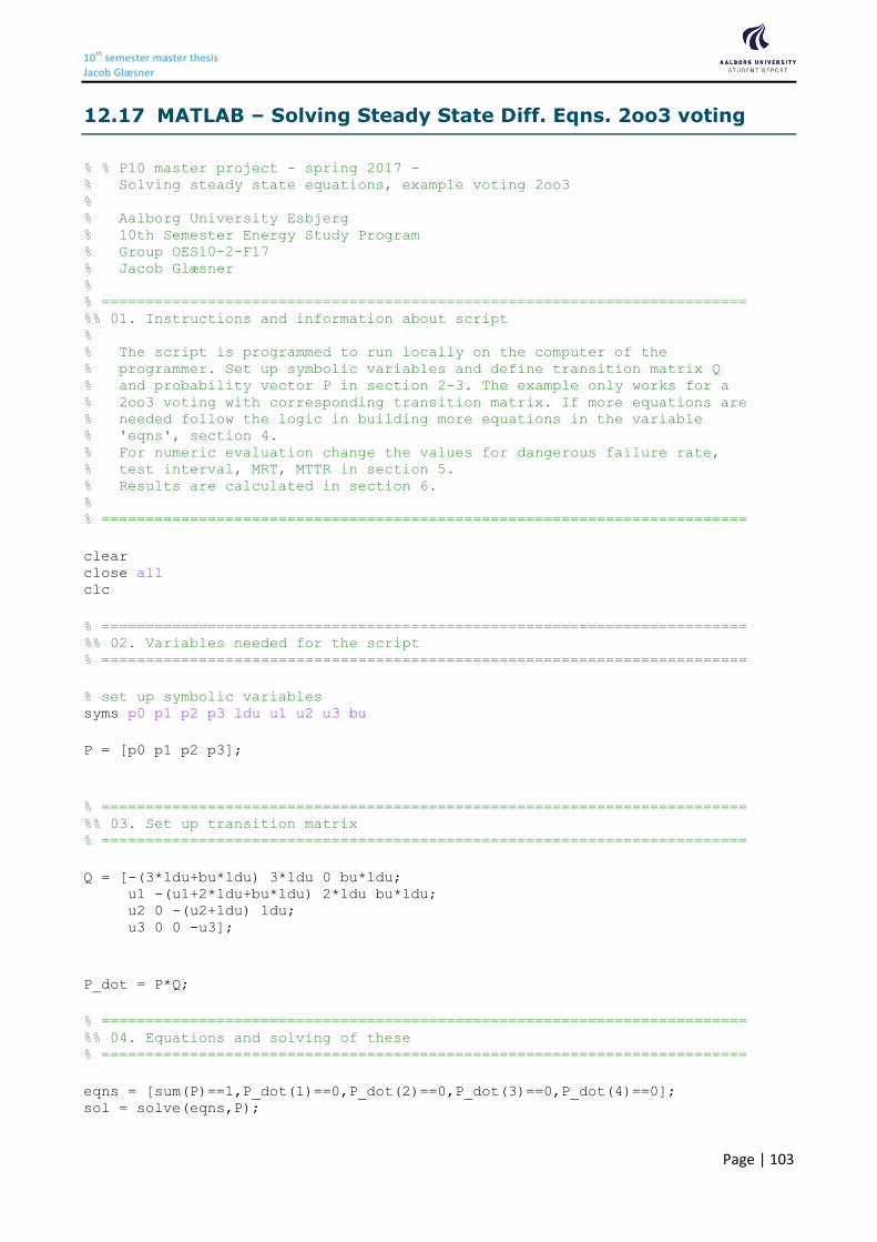
10th semester master thesis Jacob Glæsner
Page | 103
12.17 MATLAB – Solving Steady State Diff. Eqns. 2oo3 voting
% % P10 master project - spring 2017 - % Solving steady state equations, example voting 2oo3 % % Aalborg University Esbjerg % 10th Semester Energy Study Program % Group OES10-2-F17 % Jacob Glæsner % % ========================================================================= %% 01. Instructions and information about script % % The script is programmed to run locally on the computer of the % programmer. Set up symbolic variables and define transition matrix Q % and probability vector P in section 2-3. The example only works for a % 2oo3 voting with corresponding transition matrix. If more equations are % needed follow the logic in building more equations in the variable % 'eqns', section 4. % For numeric evaluation change the values for dangerous failure rate, % test interval, MRT, MTTR in section 5. % Results are calculated in section 6. % % =========================================================================
clear close all clc
% ========================================================================= %% 02. Variables needed for the script % =========================================================================
% set up symbolic variables syms p0 p1 p2 p3 ldu u1 u2 u3 bu
P = [p0 p1 p2 p3];
% ========================================================================= %% 03. Set up transition matrix % =========================================================================
Q = [-(3*ldu+bu*ldu) 3*ldu 0 bu*ldu; u1 -(u1+2*ldu+bu*ldu) 2*ldu bu*ldu; u2 0 -(u2+ldu) ldu; u3 0 0 -u3];
P_dot = P*Q;
% ========================================================================= %% 04. Equations and solving of these % =========================================================================
eqns = [sum(P)==1,P_dot(1)==0,P_dot(2)==0,P_dot(3)==0,P_dot(4)==0]; sol = solve(eqns,P);
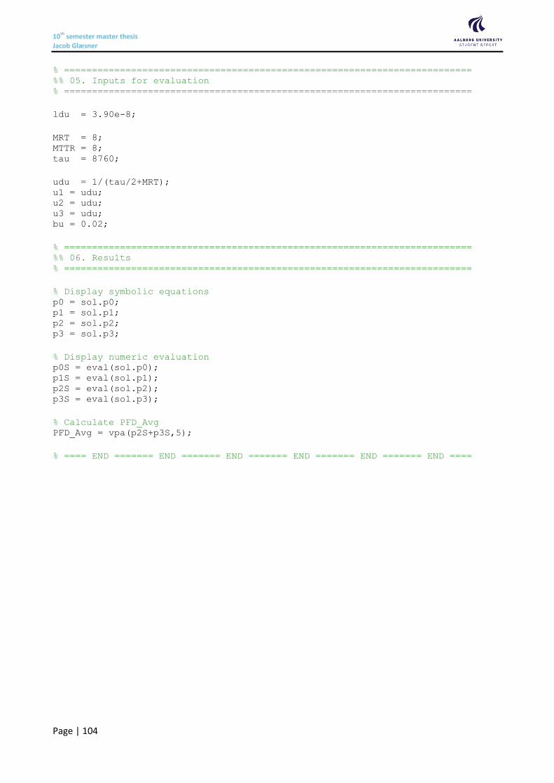
10th semester master thesis Jacob Glæsner
Page | 104
% ========================================================================= %% 05. Inputs for evaluation % =========================================================================
ldu = 3.90e-8;
MRT = 8; MTTR = 8; tau = 8760;
udu = 1/(tau/2+MRT); u1 = udu; u2 = udu; u3 = udu; bu = 0.02;
% ========================================================================= %% 06. Results % =========================================================================
% Display symbolic equations p0 = sol.p0; p1 = sol.p1; p2 = sol.p2; p3 = sol.p3;
% Display numeric evaluation p0S = eval(sol.p0); p1S = eval(sol.p1); p2S = eval(sol.p2); p3S = eval(sol.p3);
% Calculate PFD_Avg PFD_Avg = vpa(p2S+p3S,5);
% ==== END ======= END ======= END ======= END ======= END ======= END ====
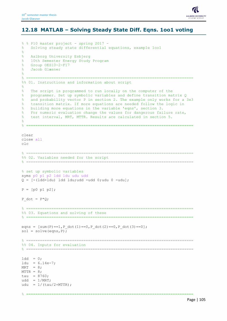
10th semester master thesis Jacob Glæsner
Page | 105
12.18 MATLAB – Solving Steady State Diff. Eqns. 1oo1 voting
% % P10 master project - spring 2017 - % Solving steady state differential equations, example 1oo1 % % Aalborg University Esbjerg % 10th Semester Energy Study Program % Group OES10-2-F17 % Jacob Glæsner % % ========================================================================= %% 01. Instructions and information about script % % The script is programmed to run locally on the computer of the % programmer. Set up symbolic variables and define transition matrix Q % and probability vector P in section 2. The example only works for a 3x3 % transition matrix. If more equations are needed follow the logic in % building more equations in the variable 'eqns', section 3. % For numeric evaluation change the values for dangerous failure rate, % test interval, MRT, MTTR. Results are calculated in section 5. % % =========================================================================
clear close all clc
% ========================================================================= %% 02. Variables needed for the script % =========================================================================
% set up symbolic variables syms p0 p1 p2 ldd ldu udu udd Q = [-(ldd+ldu) ldd ldu;udd -udd 0;udu 0 -udu];
P = [p0 p1 p2];
P_dot = P*Q;
% ========================================================================= %% 03. Equations and solving of these % =========================================================================
eqns = [sum(P)==1,P_dot(1)==0,P_dot(2)==0,P_dot(3)==0]; sol = solve(eqns,P);
% ========================================================================= %% 04. Inputs for evaluation % =========================================================================
ldd = 0; ldu = 6.14e-7; MRT = 8; MTTR = 8; tau = 8760; udd = 1/MRT; udu = 1/(tau/2+MTTR);
% =========================================================================
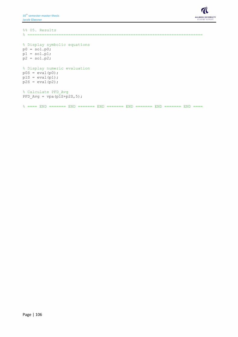
10th semester master thesis Jacob Glæsner
Page | 106
%% 05. Results % =========================================================================
% Display symbolic equations p0 = sol.p0; p1 = sol.p1; p2 = sol.p2;
% Display numeric evaluation p0S = eval(p0); p1S = eval(p1); p2S = eval(p2);
% Calculate PFD_Avg PFD_Avg = vpa(p1S+p2S,5);
% ==== END ======= END ======= END ======= END ======= END ======= END ====

10th semester master thesis Jacob Glæsner
Page | 107
12.19 MATLAB – Solving Steady State Diff. Eqns. 1oo2 voting
% % P10 master project - spring 2017 - % Solving steady state differential equations, example voting 1oo2 % % Aalborg University Esbjerg % 10th Semester Energy Study Program % Group OES10-2-F17 % Jacob Glæsner % % ========================================================================= %% 01. Instructions and information about script % % The script is programmed to run locally on the computer of the % programmer. Set up symbolic variables and define transition matrix Q % and probability vector P in section 2-3. The example only works for a % 1oo2 voting with corresponding transition matrix. If more equations are % needed follow the logic in building more equations in the variable % 'eqns', section 4. % For numeric evaluation change the values for dangerous failure rate, % test interval, MRT, MTTR in section 5. % Results are calculated in section 6. % % =========================================================================
clear close all clc
% ========================================================================= %% 02. Variables needed for the script % =========================================================================
% set up symbolic variables syms bu bd ldu1 ldu2 ldd1 ldd2 udd udu syms p0 p1 p2 p3 p4 p5 p6 p7 p8 p9
P = [p0 p1 p2 p3 p4 p5 p6 p7 p8 p9];
% ========================================================================= %% 03. Set up transition matrix % =========================================================================
Q = [-((1-bu)*ldu1 + (1-bd)*ldd1 + (1-bu)*ldu2 + (1-bd)*ldd2 +... bd*sqrt(ldd1*ldd2) + bu*sqrt(ldu1*ldu2)) (1-bu)*ldu1 (1-bd)*ldd1... (1-bu)*ldu2 (1-bd)*ldd2 0 0 0 bd*sqrt(ldd1*ldd2) bu*sqrt(ldu1*ldu2);... udu (-udu-ldu2-ldd2) 0 0 0 ldu2 0 ldd2 0 0;... udd 0 (-udd-ldu2-ldd2) 0 0 0 ldu2 0 ldd2 0;... udu 0 0 -(udu+ldu1+ldd1) 0 ldu1 ldd1 0 0 0;... udd 0 0 0 -(udd+ldu1+ldd1) 0 0 ldu1 ldd1 0;... udu 0 0 0 0 -udu 0 0 0 0;... 0 0 udu udd 0 0 -udu-udd 0 0 0;... 0 udd 0 0 udu 0 0 -udd-udu 0 0;... 0 0 udd 0 udd 0 0 0 -2*udd 0;... udu 0 0 0 0 0 0 0 0 -udu];
P_dot = P*Q;
% =========================================================================
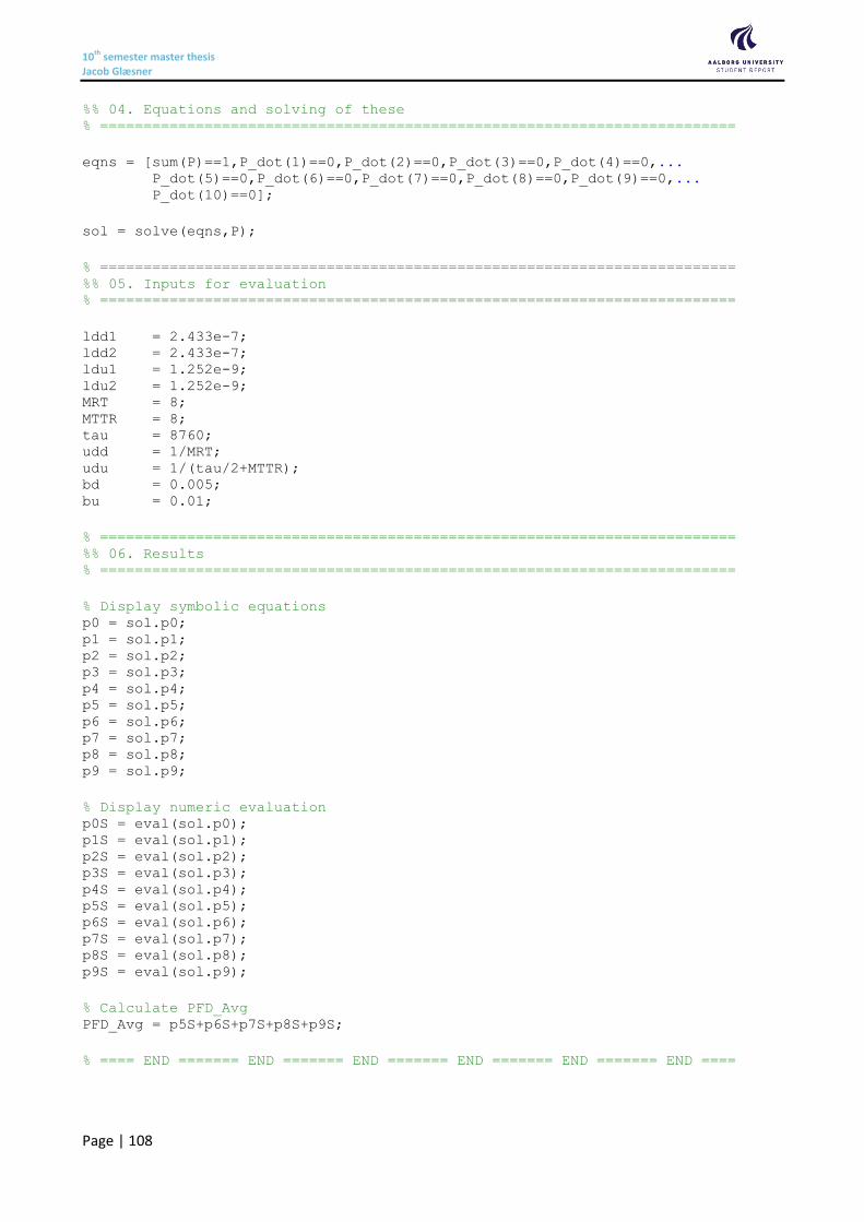
10th semester master thesis Jacob Glæsner
Page | 108
%% 04. Equations and solving of these % =========================================================================
eqns = [sum(P)==1,P_dot(1)==0,P_dot(2)==0,P_dot(3)==0,P_dot(4)==0,... P_dot(5)==0,P_dot(6)==0,P_dot(7)==0,P_dot(8)==0,P_dot(9)==0,... P_dot(10)==0];
sol = solve(eqns,P);
% ========================================================================= %% 05. Inputs for evaluation % =========================================================================
ldd1 = 2.433e-7; ldd2 = 2.433e-7; ldu1 = 1.252e-9; ldu2 = 1.252e-9; MRT = 8; MTTR = 8; tau = 8760; udd = 1/MRT; udu = 1/(tau/2+MTTR); bd = 0.005; bu = 0.01;
% ========================================================================= %% 06. Results % =========================================================================
% Display symbolic equations p0 = sol.p0; p1 = sol.p1; p2 = sol.p2; p3 = sol.p3; p4 = sol.p4; p5 = sol.p5; p6 = sol.p6; p7 = sol.p7; p8 = sol.p8; p9 = sol.p9;
% Display numeric evaluation p0S = eval(sol.p0); p1S = eval(sol.p1); p2S = eval(sol.p2); p3S = eval(sol.p3); p4S = eval(sol.p4); p5S = eval(sol.p5); p6S = eval(sol.p6); p7S = eval(sol.p7); p8S = eval(sol.p8); p9S = eval(sol.p9);
% Calculate PFD_Avg PFD_Avg = p5S+p6S+p7S+p8S+p9S;
% ==== END ======= END ======= END ======= END ======= END ======= END ====
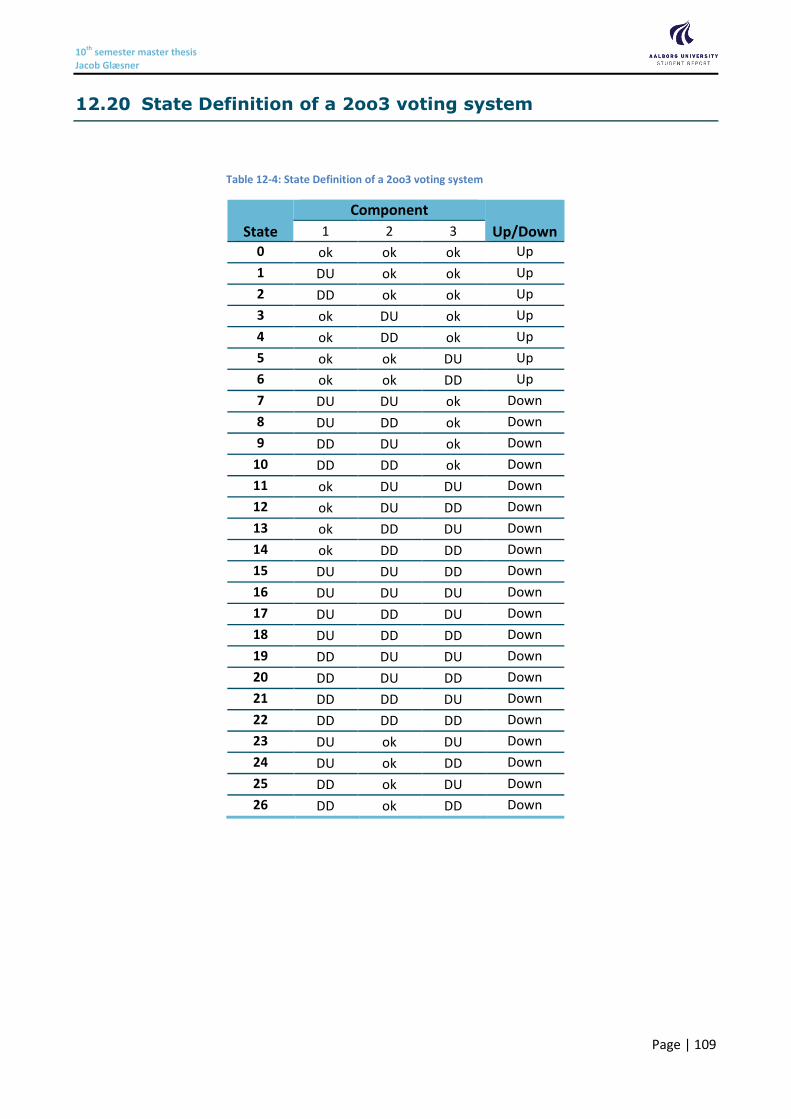
10th semester master thesis Jacob Glæsner
Page | 109
12.20 State Definition of a 2oo3 voting system
Table 12-4: State Definition of a 2oo3 voting system
State
Component
Up/Down 1 2 3
0 ok ok ok Up
1 DU ok ok Up
2 DD ok ok Up
3 ok DU ok Up
4 ok DD ok Up
5 ok ok DU Up
6 ok ok DD Up
7 DU DU ok Down
8 DU DD ok Down
9 DD DU ok Down
10 DD DD ok Down
11 ok DU DU Down
12 ok DU DD Down
13 ok DD DU Down
14 ok DD DD Down
15 DU DU DD Down
16 DU DU DU Down
17 DU DD DU Down
18 DU DD DD Down
19 DD DU DU Down
20 DD DU DD Down
21 DD DD DU Down
22 DD DD DD Down
23 DU ok DU Down
24 DU ok DD Down
25 DD ok DU Down
26 DD ok DD Down

![e-beam [F17] LVL is a direct substitute for F17 hardwood at competitive … · 2017-08-29 · e-beam+ [F17] LVL is a direct substitute for F17 hardwood at competitive prices and is](https://img.pdfslide.net/doc/110x75/5f43fc49ddb8f2221b04a783/e-beam-f17-lvl-is-a-direct-substitute-for-f17-hardwood-at-competitive-2017-08-29.jpg)
![e-beam [F17] LVL is a direct substitute for F17 hardwood at … Documents... · 2016-06-27 · e-beam+ [F17] LVL is a direct substitute for F17 hardwood at competitive prices and](https://img.pdfslide.net/doc/110x75/5f7b53a68440c74fd0043c36/e-beam-f17-lvl-is-a-direct-substitute-for-f17-hardwood-at-documents-2016-06-27.jpg)