November 2012 1 P2

Management Level Paper

P2 – Performance Management November 2012 examination

Examiner’s Answers

Note: Some of the answers that follow are fuller and more comprehensive than would be expected from a well-prepared candidate. They have been written in this way to aid teaching, study and revision for tutors and candidates alike. These Examiner’s answers should be reviewed alongside the question paper for this examination which is now available on the CIMA website at www.cimaglobal.com/p2papers The Post Exam Guide for this examination, which includes the marking guide for each question, will be published on the CIMA website by early February at www.cimaglobal.com/P2PEGS

SECTION A Answer to Question One Rationale The question examines candidates’ knowledge, understanding and application of variance analysis linked to the learning curve. The learning outcome tested is B1 (e), apply learning curves to estimate time and cost for new products and services. Suggested Approach Carefully read and absorb the data provided, and by use of either the labour efficiency planning variance, or the labour efficiency operating variance, calculate the revised standard time to produce 32 units. The next step needed a calculation to arrive at the average time per unit, and express this as a percentage of the time for the first unit (25 hours). Then, by recognising that the number of ‘ doublings’ is five, take the fifth root of the percentage earlier calculated to arrive at the expected learning rate. Part (b) requested you to explain two reasons why it is important for production and control purposes to identify the learning curve, such as scheduling, control and resourcing.

(a) The planning variance is $4,320. This represents 360 hours. Therefore the revised

standard time to produce 32 units is (25*32) - 360 = 440 hours.

The cumulative average standard time per unit is 440/32 = 13.75 hours per unit

www.theallpapers.com

P2 2 November 2012

The time for the first unit was 25 hours. The cumulative average time per unit for the first 32 units as a percentage of the time for the first unit is 55%. 32 units is 5 doublings of output (2, 4, 8, 16, 32) and therefore 55% is the fifth root of the learning rate Therefore the expected learning rate was 88.7%

(b) The identification of the learning curve is important because of its impact on the time

taken to produce the output. This has implications in many areas of production planning and control: Scheduling: it is important to know the expected time that the output will take so that realistic schedules can be produced. This is important for meeting deadlines and also for effective utilisation of resources (for example preventing under utilisation of capacity). Resources: production planning is needed to ensure that sufficient resources are available (e.g. materials). If the workers can work faster because of the learning curve it is important that the resources they need are available. Control: if the learning curve is not identified, the efficiency variance is of little use for control purposes. The impact of the learning curve will hide the true picture of the labour efficiency variance because the ‘standard’ will be unrealistic if it is based on the time taken for the first unit to be produced. Note: the question asked for two reasons. Marks were awarded for reasons other than those shown above.

Answer to Question Two Rationale The question examines candidates’ knowledge and understanding of a flexed budget. The learning outcome tested is C2 (c), evaluate performance using fixed and flexible budget reports. Suggested Approach Carefully read and digest the relevant information and produce an amended statement that includes a flexed budget column. The variance column would now compare the flexed budget with the actual column. Part (b) asked for an explanation of a benefit and a limitation of the statement produced in part (a).

www.theallpapers.com

November 2012 3 P2

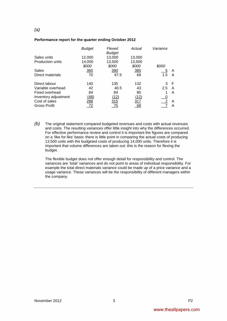
(a) Performance report for the quarter ending October 2012 Budget Flexed

Budget Actual Variance

Sales units 12,000 13,000 13,000 Production units 14,000 13,500 13,500 $000 $000 $000 $000 Sales 360 390 385 A 5 Direct materials 70 67.5 69 1.5 A

Direct labour 140 135 132 3 F Variable overhead 42 40.5 43 2.5 A Fixed overhead 84 84 85 1 A Inventory adjustment (48) (12) (12) 0 Cost of sales 288 315 317 A 2 Gross Profit 72 75 68 A 7 (b) The original statement compared budgeted revenues and costs with actual revenues

and costs. The resulting variances offer little insight into why the differences occurred. For effective performance review and control it is important the figures are compared on a ‘like for like’ basis: there is little point in comparing the actual costs of producing 13,500 units with the budgeted costs of producing 14,000 units. Therefore it is important that volume differences are taken out: this is the reason for flexing the budget.

The flexible budget does not offer enough detail for responsibility and control. The variances are ‘total’ variances and do not point to areas of individual responsibility. For example the total direct materials variance could be made up of a price variance and a usage variance. These variances will be the responsibility of different managers within the company.

www.theallpapers.com

P2 4 November 2012

Answer to Question Three Rationale The question examines candidates’ knowledge of participative budgeting. The learning outcome tested is C3 (a), discuss the impact of budgetary control systems and setting of standard costs on human behaviour. Suggested Approach Carefully read the scenario to identify the circumstances associated with the introduction of a participative budget. A report addressed to the new Director was required that needed to contain specific items such as potential benefits and disadvantages of involving new managers in this budget setting process. Finally the question asked for a recommendation to the new Director relating to the introduction of a participative budget. REPORT To: Managing Director From: XX Subject: Participative budgeting. Date: November 2012 Introduction The following report identifies two advantages and two disadvantages of involving managers in the setting of budgets. Advantages 1) If managers are involved in setting budgets then the budgets may be more relevant to the

business because the manager will have specialist knowledge of their area of the business and they can incorporate this into their budgets. As a result the budgets will provide a more realistic target and are a better indicator of likely results which can then be used in strategic planning and decision making with a view to meeting the terms of the contract.

2) If managers are involved in the budget setting process then they are likely to take ownership of the budget and feel that failing to achieve it is a personal failure. This means that managers will be motivated to achieve the targets they have set and agreed, and consequently the target is more likely to be achieved than one that is simply handed to them without their involvement.

3) The new managers may gain valuable knowledge of the business by working closely with the existing managers when preparing the budgets. The existing managers may have detailed knowledge of current operations and the availability of resources that are of benefit for the new contract.

Disadvantages 1) The managers may deliberately set themselves targets that are easier to achieve by the

inclusion of budgetary slack. This may result in the company’s performance being lower than it would have been had more difficult targets been imposed on the managers. However targets are set in the contract.

2) Some of the managers may have less experience than others in managing passenger transport operations. Consequently they may not understand the relationships that exist between different budgets and the impact that one has on the other and they may take decisions in their own area that are detrimental to another area of the business and to the company as a whole.

www.theallpapers.com

November 2012 5 P2

Recommendation It is important that the managers work together as a team to prepare the company’s budgets. In this way they can share their expertise and produce a set of budgets that are realistic and for the benefit of the company as a whole. In this way it is generally agreed that manager involvement in the budget setting process is likely to lead to better budgets and better performance. Answer to Question Four Rationale The question examines candidates’ knowledge and understanding of quality costs. The learning outcome tested is B1 (d), prepare cost of quality reports. Suggested Approach Part (a) required an explanation of each of the four quality cost classifications using examples from the scenario. Part (b) required a discussion, using data from the scenario, to describe the relationship between conformance costs and non-conformance costs and its importance to this company.

(a) Prevention costs are costs that are incurred in order to prevent poor quality.

Examples from the data provided are expenditure on staff training and preventative maintenance.

Appraisal costs are costs incurred to measure or appraise the quality of the items produced. An example from the data provided is finished goods inspection cost. Internal failure costs are costs that are incurred in rejecting or correcting faulty goods where the quality failure is discovered before the item is despatched to the customer. An example from the data provided would be the costs related to the goods that are rejected before delivery. External failure costs are costs that are incurred as a result of customers rejecting goods that have been delivered to them. In the data provided there are goods that have been rejected by customers. The costs associated with these rejects would include collection and re-delivery costs and the loss of customer goodwill.

(b) Conformance costs are prevention and appraisal costs. Non-conformance costs are

internal and external failure costs. The relationship is that higher conformance costs should in the long run lead to lower non-conformance costs.

In the data provided it can be seen that costs incurred on prevention and appraisal costs were a greater percentage of turnover in 2012 compared to 2011 and as a result the level of external failures reduced. This would improve the perception of the company in the market.

It can also be seen that the level of failures identified before despatch increased. This could be because of the greater expenditure on appraisal costs. However it would appear that there are far too many ‘rejects’ being manufactured and that the company needs to work towards improving the quality of its manufacturing processes rather than relying on quality inspections to identify sub-standard production. The company should work towards ‘designing quality in’ as opposed to ‘inspecting poor quality out’.

www.theallpapers.com

P2 6 November 2012

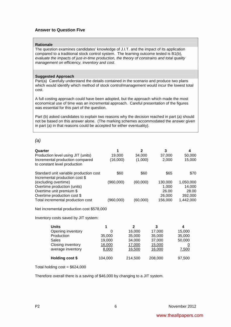
Answer to Question Five Rationale The question examines candidates’ knowledge of J.I.T. and the impact of its application compared to a traditional stock control system. The learning outcome tested is B1(b), evaluate the impacts of just-in-time production, the theory of constrains and total quality management on efficiency, inventory and cost. Suggested Approach Part(a) Carefully understand the details contained in the scenario and produce two plans which would identify which method of stock control/management would incur the lowest total cost. A full costing approach could have been adopted, but the approach which made the most economical use of time was an incremental approach. Careful presentation of the figures was essential for this part of the question. Part (b) asked candidates to explain two reasons why the decision reached in part (a) should not be based on this answer alone. (The marking schemes accommodated the answer given in part (a) in that reasons could be accepted for either eventuality). (a) Quarter 1 2 3 4 Production level using JIT (units) 19,000 34,000 37,000 50,000 Incremental production compared to constant level production

(16,000) (1,000) 2,000 15,000

Standard unit variable production cost $60 $60 $65 $70 Incremental production cost $ (excluding overtime)

(960,000)

(60,000)

130,000

1,050,000

Overtime production (units) 1,000 14,000 Overtime unit premium $ 26.00 28.00 Overtime production cost $ 26,000 392,000 Total incremental production cost (960,000) (60,000) 156,000 1,442,000 Net incremental production cost $578,000 Inventory costs saved by JIT system:

Units 1 2 3 4 Opening inventory 0 16,000 17,000 15,000 Production 35,000 35,000 35,000 35,000 Sales 19,000 34,000 37,000 50,000 Closing inventory 16,000 17,000 0 15,000 average inventory 8,000 16,500 16,000

7,500

Holding cost $ 104,000 214,500 208,000 97,500 Total holding cost = $624,000 Therefore overall there is a saving of $46,000 by changing to a JIT system.

www.theallpapers.com

November 2012 7 P2

(b) On the basis of the above calculations CDE should change to a JIT production system

but there are other factors that should be considered:

How long is the contract? What will the demand be for next year and subsequent years given the important features of the component? It would be foolish to make the decision based only on the first year’s forecast if this is to be a long term contract. A full investment appraisal should be undertaken and the decision should be based on the net present value of the relevant cash flows. Overtime will be needed in the final two quarters. Given the rising costs and the overtime premium, can alternative methods of production be found? What will be the impact of the overtime working on the workforce? In a JIT production system there will be no inventory and consequently there is no margin for errors in production. Consequently CDE may need to invest in quality control systems in order to ensure that the units produced are of the appropriate quality. Note: the question asked for two factors. Marks were awarded to other relevant comments.

www.theallpapers.com

P2 8 November 2012

SECTION B Answer to Question Six Rationale The question examines candidates’ knowledge and understanding of limiting factors, aspects associated with limiting factors, such as make v buy, and break even analysis. The learning outcomes tested are: part (a) A2 (b), apply and interpret variable/fixed cost analysis in multiple product contexts to break-even analysis and product mix decisions, including circumstances where there are multiple constrains and linear programming methods needed to identify ‘optimal’ solutions; part (b) A2(c), discuss the meaning of ‘optimal’ solutions and demonstrate how linear programming methods can be employed for profit maximising, revenue maximising and satisfying objective; parts (c) and (d), A2(d), analyse the impact of uncertainty and risk on decision models based on CPV analysis. Suggested Approach Part (a) carefully read the question to fully understand the details provided and what was required. The first step was to establish the limiting factor and then construct a table to allow the company to arrive at a production plan that would maximise the company’s profit. It was important that products C1 and C2 were treated in exactly the same way as the treatment for products P1, P2 and P3. Part (b) required a sound understanding of shadow pricing, before addressing the figures given in the question. Part (c) required an understanding of breakeven analysis when faced with products which are sold in a specific ratio. Part (d) used the same scenario as part (c) but required the ability to calculate the sensitivity of one of the products. Part (d) was not reliant on the completion of part (c). (a) Resource requirements for internal production of all units demanded:

Direct labour (hours)

Direct materials

(kg) P1 (500 units) 1,250 100 P2 (400 units) 600 160 P3 (600 units) 1,800 240 C1 (250 units) 250 25 C2 (150 units) 225 Total

30 4,125

Available 555

4,300 420

As can be seen the direct materials are the scarce resource so the ranking is based on the contribution per kg of direct materials.

www.theallpapers.com

November 2012 9 P2

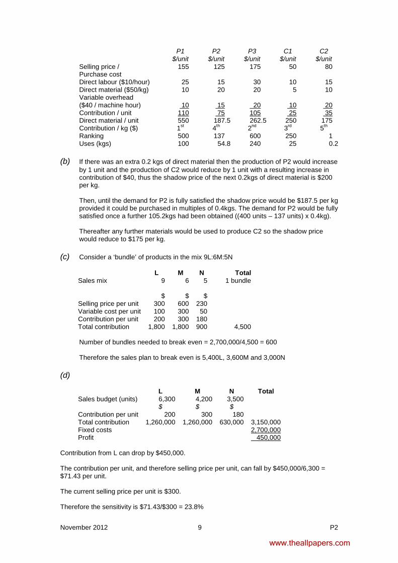
P1 $/unit

P2 $/unit

P3 $/unit

C1 $/unit

C2 $/unit

Selling price / Purchase cost

155 125 175 50 80

Direct labour ($10/hour) 25 15 30 10 15 Direct material ($50/kg) 10 20 20 5 10 Variable overhead ($40 / machine hour)

10

15

20

10

Contribution / unit 20

110 75 105 25 Direct material / unit

35 550 187.5 262.5 250 175

Contribution / kg ($) 1st 4th 2nd 3rd 5th Ranking 500 137 600 250 1 Uses (kgs) 100 54.8 240 25 0.2

(b) If there was an extra 0.2 kgs of direct material then the production of P2 would increase

by 1 unit and the production of C2 would reduce by 1 unit with a resulting increase in contribution of $40, thus the shadow price of the next 0.2kgs of direct material is $200 per kg.

Then, until the demand for P2 is fully satisfied the shadow price would be $187.5 per kg provided it could be purchased in multiples of 0.4kgs. The demand for P2 would be fully satisfied once a further 105.2kgs had been obtained ((400 units – 137 units) x 0.4kg).

Thereafter any further materials would be used to produce C2 so the shadow price would reduce to $175 per kg.

(c) Consider a ‘bundle’ of products in the mix 9L:6M:5N

L M N Total Sales mix 9 6 5 1 bundle $ $ $ Selling price per unit 300 600 230 Variable cost per unit 100 300 50 Contribution per unit 200 300 180 Total contribution 1,800 1,800 900 4,500

Number of bundles needed to break even = 2,700,000/4,500 = 600

Therefore the sales plan to break even is 5,400L, 3,600M and 3,000N

(d)

L M N Total Sales budget (units) 6,300 4,200 3,500 $ $ $ Contribution per unit 200 300 180 Total contribution 1,260,000 1,260,000 630,000 3,150,000 Fixed costs Profit

2,700,000

450,000

Contribution from L can drop by $450,000. The contribution per unit, and therefore selling price per unit, can fall by $450,000/6,300 = $71.43 per unit. The current selling price per unit is $300. Therefore the sensitivity is $71.43/$300 = 23.8%

www.theallpapers.com

P2 10 November 2012

Answer to Question Seven Rationale The question examines candidates’ understanding of transfer pricing, the calculation of the maximum profit for a division and the company as a whole, and a discussion on transfer pricing using opportunity cost. The learning outcomes tested are: part (a) and part(c), D3(c), discuss the likely consequences of different approaches to transfer pricing for divisional decision making and group profitability, the motivation of divisional management and the autonomy of individual divisions. Part (b), D2(b), prepare and discuss revenue and cost information in appropriate formats for profit and investment centre managers taking due account of cost viability, attributable costs, controllable costs, and identification of appropriate measures of profit centre ‘contribution’. Suggested Approach Part (a)(i) Carefully digest the details in the question and calculate the revenue generated by the complete cameras when viewed by the Optics divisional manager. The main aim was to calculate the selling price the Optics division would transfer the optical device to the Body division. Part (a)(ii) a required similar calculations but the transfer price needed to generate the maximum profit for the OB group. Part (b) considered the transfer of items between two divisions of the same company and required calculations to address the two situations described in the questions. Part (c) required a discussion relating to the use of opportunity costs as a basis for transfer pricing. All parts of this question required answers to relate to the scenarios in the question. (a)

(i) Optics division Price equation is P = 6,000 – 0.5x

Profit maximised when MC = MR 1,200 = 6,000 – x x = 4,800 Therefore P = 6,000 – 2,400 = $3,600 Body Division Price equation is P = 8,000 – (1/3)x Profit maximised when MC = MR The marginal cost for the complete camera will be 1,750 + 3,600 = 5,350 5,350 = 8,000 – (2/3)x (2/3)x = 2,650 x = 3,975 P = 8,000 – (1/3)3,975 P = $6,675 Revenue generated by the complete cameras = 3,975 * $6,675 = $26,533,125

www.theallpapers.com

November 2012 11 P2

(ii) If the transfer price was set to maximise the profits of the group it would be $1,200 and

the marginal cost of a complete camera would be $2,950

MC = MR 2,950 = 8,000 – (2/3)x (2/3)x = 5,050 x = 7,575 P = 8,000 – (1/3)7,575 P = $5,475 Revenue generated by the complete cameras = 7,575 * $5,475 = $41,473,125

(b)

(i) Return required by PD = $2.4m * 12% = $288,000

Therefore total contribution needed = $2,688,000 Total contribution = (x – 1.40) * 4,480,000 2,688,000 = (x – 1.40) * 4,480,000 x – 1.40 = 2,688,000/4,480,000 = 0.60 Therefore the minimum selling price per box that PD would be willing to charge is $2.00.

(ii) Return required by SD = $6m * 12% = 720,000

Total contribution needed = $6,720,000 6,720,000 = 13,500,000 – (x * 500,000) x*500,000 = 6,780,000 x = 13.56 The maximum variable cost that would allow SD to earn a return of 12% is $13.56. The variable costs from within SD are $12.00 and therefore the maximum that it would be willing to pay for a box is $1.56

(c) The possible extreme transfer prices are:

Marginal cost: no ‘reward’ is given to the supplying division. This method could be acceptable to the supplying division if there was spare capacity but there would be a reluctance to trade at this price because of the lack of a reward. Under this system PD would supply the boxes to SD at $1.40 each. However PD is operating very close to capacity and if demand from external customers increased the opportunity cost would be the external sales that would be forgone. Market price: this should be used if there is a perfectly competitive market. The selling division will, if operating efficiently, be expected to earn a profit and the buying division should be happy to buy at this price as the only alternative is the open market. The price should be reduced for any ‘internal’ savings. This is what PD wants to do (charge SD the external selling price).

www.theallpapers.com

P2 12 November 2012

Using opportunity cost as the transfer price would enable the above extremes to be recognised. Therefore the view of the Manager of SD is worthy of support. If PD can sell all of its output externally then the opportunity cost would be the selling price. Consequently PD should not be penalised by having to accept a lower price from SD. If there is spare capacity then SD should be allowed to benefit and could then be charged just the marginal cost. However the performance appraisal will have an impact on the behaviours of the managers and their willingness to ‘trade’ must be considered. One solution to this could be to use a ‘dual pricing’ system.

www.theallpapers.com