Package ‘adehabitatHS’ - R · 2020-01-13 · bighorn 3 bighorn Radio-Tracking of Bighorn Sheeps Description This data set describes the habitat use and availability for 6 bighorn

Package ‘adehabitatHS’January 13, 2020

Version 0.3.15

Date 2020-01-11

Depends R (>= 3.0.1), sp, methods, ade4, adehabitatMA, adehabitatHR

Suggests maptools, tkrplot, MASS, rgeos

Imports graphics, grDevices, stats

Title Analysis of Habitat Selection by Animals

Author Clement Calenge, contributions from Mathieu Basille

Maintainer Clement Calenge <[email protected]>

Description A collection of tools for the analysis of habitat selection.

License GPL (>= 2)

NeedsCompilation yes

Repository CRAN

Date/Publication 2020-01-13 19:10:02 UTC

R topics documented:bauges . . . . . . . . . . . . . . . . . . . . . . . . . . . . . . . . . . . . . . . . . . . . 2bighorn . . . . . . . . . . . . . . . . . . . . . . . . . . . . . . . . . . . . . . . . . . . 3biv.test . . . . . . . . . . . . . . . . . . . . . . . . . . . . . . . . . . . . . . . . . . . . 3canomi . . . . . . . . . . . . . . . . . . . . . . . . . . . . . . . . . . . . . . . . . . . . 5chamois . . . . . . . . . . . . . . . . . . . . . . . . . . . . . . . . . . . . . . . . . . . 7compana . . . . . . . . . . . . . . . . . . . . . . . . . . . . . . . . . . . . . . . . . . . 8domain . . . . . . . . . . . . . . . . . . . . . . . . . . . . . . . . . . . . . . . . . . . 11dunnfa . . . . . . . . . . . . . . . . . . . . . . . . . . . . . . . . . . . . . . . . . . . . 13eisera . . . . . . . . . . . . . . . . . . . . . . . . . . . . . . . . . . . . . . . . . . . . 16enfa . . . . . . . . . . . . . . . . . . . . . . . . . . . . . . . . . . . . . . . . . . . . . 19engen2008II . . . . . . . . . . . . . . . . . . . . . . . . . . . . . . . . . . . . . . . . . 22gnesfa . . . . . . . . . . . . . . . . . . . . . . . . . . . . . . . . . . . . . . . . . . . . 28histniche . . . . . . . . . . . . . . . . . . . . . . . . . . . . . . . . . . . . . . . . . . . 34kselect . . . . . . . . . . . . . . . . . . . . . . . . . . . . . . . . . . . . . . . . . . . . 36madifa . . . . . . . . . . . . . . . . . . . . . . . . . . . . . . . . . . . . . . . . . . . . 39mahasuhab . . . . . . . . . . . . . . . . . . . . . . . . . . . . . . . . . . . . . . . . . 45

1

2 bauges

niche.test . . . . . . . . . . . . . . . . . . . . . . . . . . . . . . . . . . . . . . . . . . 46pheasant . . . . . . . . . . . . . . . . . . . . . . . . . . . . . . . . . . . . . . . . . . . 48predict.enfa . . . . . . . . . . . . . . . . . . . . . . . . . . . . . . . . . . . . . . . . . 49puech . . . . . . . . . . . . . . . . . . . . . . . . . . . . . . . . . . . . . . . . . . . . 50puechdesIII . . . . . . . . . . . . . . . . . . . . . . . . . . . . . . . . . . . . . . . . . 51rand.kselect . . . . . . . . . . . . . . . . . . . . . . . . . . . . . . . . . . . . . . . . . 52randtest.enfa . . . . . . . . . . . . . . . . . . . . . . . . . . . . . . . . . . . . . . . . . 54scatter.enfa . . . . . . . . . . . . . . . . . . . . . . . . . . . . . . . . . . . . . . . . . 55scatterniche . . . . . . . . . . . . . . . . . . . . . . . . . . . . . . . . . . . . . . . . . 58squirrel . . . . . . . . . . . . . . . . . . . . . . . . . . . . . . . . . . . . . . . . . . . 59squirreloc . . . . . . . . . . . . . . . . . . . . . . . . . . . . . . . . . . . . . . . . . . 60vanoise . . . . . . . . . . . . . . . . . . . . . . . . . . . . . . . . . . . . . . . . . . . 61wi . . . . . . . . . . . . . . . . . . . . . . . . . . . . . . . . . . . . . . . . . . . . . . 61

Index 66

bauges Census of chamois (Rupicapra rupicapra) in the Bauges mountains

Description

This data set contains the relocations of 198 chamois groups in the Bauges mountains, as well asmaps of 7 environmental variables on the study area.

Usage

data(bauges)

Details

This dataset contains a subsample of the data collected by volunteers and professionals working invarious French wildlife and forest management, from 1994 to 2004 in the wildlife reserve of "lesBauges" (French Alps). Note that both the maps and the relocations have been slightly destroyed topreserve copyright on the data.

Source

Daniel Maillard, Office National de la chasse et de la faune sauvage, 95 rue Pierre Flourens, 34000Montpellier, France

Examples

data(bauges)

mimage(bauges$map)image(bauges$map, 1)points(bauges$locs)

bighorn 3

bighorn Radio-Tracking of Bighorn Sheeps

Description

This data set describes the habitat use and availability for 6 bighorn sheeps monitored by radio-tracking (Arnett et al. 1989, in Manly et al., 2003, p. 67-74). 10 habitat types are considered.

Usage

data(bighorn)

Details

The object bighorn is a list, with the following components:

used the number of resource units used by each animal (in rows) in each habitat category (incolumns).

availTrue the availability of each habitat category.

availEstimated a sample of available resource units in each habitat category.

References

Manly, B.F.J., McDonald, L.L., Thomas, D.L., McDonald, T.L. & Erickson, W.P. (2003) Resourceselection by animals - Statistical design and Analysis for field studies. Second edition. London:Kluwer academic publishers.

biv.test Bivariate Test

Description

biv.plot displays a bivariate plot. biv.test displays the results of a bivariate randomisation test.

Usage

biv.plot(dfxy, br = 10, points = TRUE, density = TRUE,kernel = TRUE, o.include = FALSE, pch, cex, col, h, sub,side = c("top", "bottom", "none"), ...)

biv.test(dfxy, point, br = 10, points = TRUE, density = TRUE,kernel = TRUE, o.include = FALSE, pch, cex, col, Pcol, h, sub,side = c("top", "bottom", "none"), ...)

4 biv.test

Arguments

dfxy a data frame with N lines (couples of values) and two columns

br a parameter used to define the numbers of breaks of the histograms. A largervalue leads to a larger number of breaks

points logical. Whether the points should be displayed

density logical. Whether the kernel density estimation should be displayed for themarginal histograms

kernel logical. Whether the kernel density estimation should be displayed for the bi-variate plot

o.include logical. If TRUE, the origin is included in the plot

pch plotting "character", i.e., symbol to use for the points. (see ?points)

cex character expansion for the points

col color code or name for the points, see ?par

h vector of bandwidths for x and y directions, used in the function kde2d of thepackage MASS. Defaults to normal reference bandwidth (see ?kde2d)

sub a character string to be inserted in the plot as a title

side if "top", the x and y scales of the grid are upside, if "bottom" they are down-side, if "none" no legend

point a vector of length 2, representing the observation to be compared with the sim-ulated values of the randomisation test

Pcol color code or name for the observed point

... further arguments passed to or from other methods

Details

biv.test is used to display the results of a bivariate randomisation test. An example of use of thefunction is provided in the function niche.test.

The x-axis of the main window corresponds to the first column of dfxy; the y-axis correspondsto the second column. Kernel density is estimated to indicate the contours of the distribution ofrandomised values. The two marginal histograms correspond to the univariate tests on each axis,for which the p-values are computed with as.randtest (package ade4, one-sided tests).

Warning

biv.plot and biv.test use the function kde2d of the package MASS.

Author(s)

Mathieu Basille <[email protected]>

See Also

as.randtest (package ade4)

canomi 5

Examples

x = rnorm(1000,2)y = 2*x+rnorm(1000,2)dfxy = data.frame(x, y)

biv.plot(dfxy)biv.plot(dfxy, points=FALSE, col="lightblue", br=20)

p = c(3, 4)biv.test(dfxy, p)biv.test(dfxy, p, points=FALSE, Pcol="darkred", col="lightblue", br=20)

canomi Canonical OMI analysis

Description

This function performs a canonical OMI analysis (outlying mean index).

Usage

canomi(dudiX, Y, scannf = TRUE, nf = 2)## S3 method for class 'canomi'print(x, ...)## S3 method for class 'canomi'plot(x, xax = 1, yax = 2, ...)

Arguments

dudiX an object of class dudi

Y a a data frame Resource units-animals according to dudiX$tab with no columnsof zero

scannf a logical value indicating whether the eigenvalues bar plot should be displayed

nf if scannf FALSE, an integer indicating the number of kept axes

x an object of class canomi returned by the function canomi

xax the number of the x-axis

yax the number of the x-axis


6 canomi

Details

The canonical OMI analysis is similar to the function niche, from the package ade4. The principleof this analysis is the following. A set of N resource units (RUs) are available to the animals ofthe study. Each resource unit is described by P environmental variables. Therefore, the N resourceunits define a cloud of N points in the P-dimensionnal space defined by the P variables. We call thisspace "ecological space".

Moreover, the use of the N resource units is known (or sampled) for a sample of K animals (e.g.,using radio-tracking). These utilization weights for each RU (rows) and each animal (column)define a table Y. For a given animal, the set of resource units used define the "niche" of the animal.The vector connecting the centroid (mean) of the available RUs to the centroid of the RUs usedby this animal is named "marginality vector" (and its squared length is named "marginality" or"outlying mean index").

The canomi first distorts the ecological space so that the available resource units take a standardspherical shape (by first performing a principal component analysis). Then, in this distorted space,a non-centred principal component analysis of the marginality vectors is performed. The canonicalOMI analysis finds the directions in the distorted ecological space where the marginality is, inaverage, the largest.

Value

canomi returns a list of the class canomi, with the following components:

call original call.

rank an integer indicating the rank of the studied matrix

nf an integer indicating the number of kept axes

eig a vector with all the eigenvalues of the analysis.

tab a data frame with n rows (n animals) and p columns (p environmental variables).

li animals coordinates, data frame with n rows and nf columns.

l1 animals normed coordinates, data frame with n rows and nf columns.

c1 column scores, data frame with p rows and nf columns.

cor the correlation between the canomi axes and the original variables

ls a data frame with the resource units coordinates

cm The variables metric used in the analysis (e.g. ls = dudiX$tab%*%cm%*%c1)

as a data frame with the axis upon niche axis

Author(s)

Clement Calenge <[email protected]>

References

Chessel, D. 2006. Calcul de l’outlier mean index. Consultation statistique avec le logiciel R.

See Also

dudi for class dudi, niche for classical OMI analysis

chamois 7

Examples

## The datadata(puech)locs <- puech$relocationsmaps <- puech$maps

## the mapsmimage(maps)

## the relocations of the wild boar:image(maps)points(locs, col=as.numeric(slot(locs, "data")[,1]))

## count the number of relocations## in each pixel of the mapscp <- count.points(locs, maps)

## gets the data:dfavail <- slot(maps, "data")dfused <- slot(cp, "data")

## a preliminary principal component analysis of the data:dud <- dudi.pca(dfavail, scannf=FALSE)

## The analysis:nic <- canomi(dud, dfused, scannf=FALSE)nic

## Plot the results:plot(nic)

chamois Location of Chamois Groups in the Chartreuse Mountains

Description

This data set describes the habitat use and availability by the chamois of the Chartreuse mountains(Isere, France), in 1992 and 1997. These data have been gathered during the hunting season (Fall).

Usage

data(chamois)

8 compana

Details

The object chamois is a list containing the following components:

locs is a data frame containing the x and y coordinates of 198 chamois groups.

map is a map of class kasc describing the vegetation (Forest or Open areas), the distance from theecotone Open/Forest and the slopes on the area.

References

Federation Departementale des Chasseurs de l’Isere, 65 av Jean Jaures, 38320 Eybens. France.

compana Compositional Analysis of Habitat Use

Description

compana performs a classical compositional analysis of habitat use (Aebischer et al., 1993).

Usage

compana(used, avail, test = c("randomisation", "parametric"),rnv = 0.01, nrep = 500, alpha = 0.1)

Arguments

used a matrix or a data frame describing the percentage of use of habitats (in columns)by animals (in rows).

avail a matrix or a data frame describing the percentage of availability of habitats (incolumns) by animals (in rows).

test a character string. If "randomisation", randomisation tests are performed forboth the habitat ranking and the test of habitat selection. If "parametric", usualparametric tests are performed (chi-square for the test of habitat selection andt-tests for habitat ranking).

rnv the number replacing the 0 values occurring in the matrix used.

nrep the number of repetitions in the randomisation tests.

alpha the alpha level for the tests.

Details

The compositional analysis of habitat use has been recommended by Aebischer et al. (1993) for theanalysis of habitat selection by several animals, when the resources are defined by several categories(e.g. vegetation types).

This analysis is carried out in two steps: first the significance of habitat selection is tested (usinga Wilks lambda). Then, a ranking matrix is built, indicating whether the habitat type in row issignificantly used more or less than the habitat type in column. When this analysis is performedon radio-tracking data, Aebischer et al. recommend to study habitat selection at two levels: (i)

compana 9

selection of the home range within the study area, and (ii) selection of the relocations within thehome range. The first level is termed second-order habitat selection on Johnson’s scale (1980), andthe second one, third-order habitat selection.

When zero values are found in the matrix of used habitats, they are replaced by a small value (bydefault, 0.01), according to the recommendations of Aebischer et al. (1993).

When zero values are found in the matrix of available habitats, the function compana uses theprocedure termed "weighted mean lambda" described in Aebischer et al. (1993: Appendix 2),instead of the usual lambda (see examples). Zero values can be found in the matrix of availablehabitats when the third-order habitat selection is under focus. In this case, it may occur that somehabitat types are available to some animals and not to the others.

Note that this method rely on the following hypotheses: (i) independence between animals, and (ii)all animals are selecting habitat in the same way (in addition to "traditional" hypotheses in thesekinds of studies: no territoriality, all animals having equal access to all available resource units,etc.). The function eisera can be used as a preliminary to identify whether this is indeed the case(see examples).

Value

Returns a list of the class compana:

used the matrix of used habitatsavail the matrix of available habitatstype.test a character string. Either "randomisation" or "parametric"test the results of the test of habitat selectionrm the ranking matrix: a square matrix with nh rows and nh columns, where nh is

the number of habitat types under study. At the intersection of the row i andof the column j, there is a "+" when the habitat i is more used than the habitatin column, and "-" otherwise. When the difference is significant, the sign istripled.

rmnb the matrix containing the number of animals used to perform the tests in rm.rank the rank of the habitat types. It is equal to the number of "+" for each habitat

type in row of rm.rmv the matrix of statistics used to build rm. If (test = "parametric"), the matrix

contains the values of t, in the t-test comparing the row and the column habi-tat. If (test = "randomisation"), the matrix contains the mean differencebetween the used and available log-ratios (see Aebischer et al., 1993).

profile the profile of preferences: resource types are sorted so that the left type is themost preferred and the right type is the most avoided. Habitats for which theintensity of habitat selection is similar (no significant difference) are connectedby a line.

Note

In the examples below, the results differ from those published in Aebischer et al. (squirrel example,selection of the relocations within the home range). In fact, there has been a confusion in the columnnames in the paper. Actually, Aebischer (pers. com.) indicated that the ranking matrix given in thisexample is correct.

10 compana

Author(s)


References

Aebischer, N. J. and Robertson, P. A. (1992) Practical aspects of compositional analysis as appliedto pheasant habitat utilisation. pp. 285–293 In: Priede, G. and Swift, S. M. Wildlife telemetry,remote monitoring and tracking of animals.

Aebischer, N. J., Robertson, P. A. and Kenward, R. E. (1993) Compositional analysis of habitat usefrom animal radiotracking data. Ecology, 74, 1313–1325.

Johnson, D. H. (1980) The comparison of usage and availability measurements for evaluating re-source preference. Ecology, 61, 65–71.

See Also

eisera to perform an eigenanalysis of selection ratios, preliminary to the use of compositionalanalysis.

Examples

## The examples presented here## are the same as those presented in## the paper of Aebischer et al. (1993)

############################### Pheasant dataset: first## example in Aebischer et al.

data(pheasant)

## Second order habitat selection## Selection of home range within the## study area (example of parametric test)pheana2 <- compana(pheasant$mcp, pheasant$studyarea,

test = "parametric")pheana2

## The ranking matrix:print(pheana2$rm, quote = FALSE)

## Third order habitat selection## (relocation within home range)## We remove the first pheasant of the analysis## (as in the paper of Aebischer et al.)## before the analysispheana3 <- compana(pheasant$locs[-1,], pheasant$mcp[-1,c(1,2,4)])pheana3

domain 11

## The ranking matrix:print(pheana3$rm, quote = FALSE)

############################### Squirrel data set: second## example in Aebischer et al.

data(squirrel)

## Second order habitat selection## Selection of home range within the## study areasquiana2 <- compana(squirrel$mcp, squirrel$studyarea)squiana2

## The ranking matrix:print(squiana2$rm, quote = FALSE)

## However, note that here, the hypothesis of identical use## on which this analysis relies is likely to be false.## Indeed, an eisera indicates:

us <- round(30 * squirrel$locs / 100)av <- squirrel$studyareaii <- eisera(us, av, scannf = FALSE)scatter(ii, grid = FALSE, clab = 0.7)

## There are clearly two groups of animals. In such cases,## compositional analysis is to be avoided in this case.

## Third order habitat selection## (relocation within home range)## We remove the second column## (as in the paper of Aebischer et al.)squiana3 <- compana(squirrel$locs[,-2], squirrel$mcp[,-2])squiana3

## The ranking matrix:print(squiana3$rm, quote = FALSE)

domain Estimation of the Potential Distribution of a Species

12 domain

Description

domain uses the DOMAIN algorithm to estimate the potential distribution of a species based on alist of species occurrences and on maps of the area.

Usage

domain(x, pts, type = c("value", "potential"), thresh = 0.95)

Arguments

x an object of class SpatialPixelsDataFrame

pts a data frame giving the x and y coordinates of the species occurrences.

type a character string. The "value" of the suitability may be returned or the "potential"area of distribution

thresh if value = "potential", a threshold value should be supplied for the suitability(by default 0.95)

Details

This function implements the DOMAIN algorithm described in Carpenter et al. (1993).

Value

Returns an object of class SpatialPixelsDataFrame.

Warning

domain is restricted to maps containing only numerical variables (i.e. no factors).

Author(s)


References

Carpenter, G., Gillison, A.N. and Winter, J. (1993) DOMAIN: a flexible modelling procedure formapping potential distributions of plants and animals. Biodiversity and conservation, 2, 667–680.

See Also

mahasuhab

dunnfa 13

Examples

## Preparation of the datadata(lynxjura)map <- lynxjura$mappts <- lynxjura$locs

## View of the dataimage(map)title(main="Elevation")points(pts, pch = 3)

## Estimation of habitat suitability maphsm <- domain(map, pts)

image(hsm, col = grey((1:256)/256))contour(hsm, add = TRUE)

## Lighter areas are the most used areas

## Potential distributionhsm <- domain(map, pts, type = "potential", thresh = 0.98)image(hsm, col = "orange")title(main = "Habitat suitability map")points(pts, pch = 3)

dunnfa Factorial Analysis of the Specialization in Habitat Selection Studies.Unpublished Work of James Dunn (University of Arkansas)

Description

dunnfa performs a factorial decomposition of the Mahalanobis distances in habitat selection studies(see details).

Usage

dunnfa(dudi, pr, scannf = TRUE, nf = 2)## S3 method for class 'dunnfa'print(x, ...)

Arguments

dudi an object of class pca

pr a vector giving the utilization weights associated to each unit

scannf logical. Whether the eigenvalues barplot should be displayed

nf an integer indicating the number of kept axes

14 dunnfa

x an object of class dunnfa

... additional arguments to be passed to the function print

Details

This analysis is in essence very similar to the MADIFA (see ?madifa). The Mahalanobis distancesare often used in the context of niche-environment studies (Clark et al. 1993, see the functionmahasuhab). Each resource unit takes a value on a set of environmental variables. Each environ-mental variable defines a dimension in a multidimensionnal space, namely the ecological space. Aset of points (resource units) describes what is available to the species. For each point, a "utilizationweight" measures the intensity of use of the point by the species. The set of points for which theutilization weight is greater than zero defines the "niche". The Mahalanobis distance between anyresource unit in this space (e.g. the point defined by the values of environmental variables in a pixelof a raster map) and the centroid of the niche (the distribution of used resource units) can be usedto give a value of eccentricity to this point.

For a given distribution of available resource units, for which a measure of Mahalanobis distances isdesired, the MADIFA (MAhalanobis DIstances Factor Analysis) partitions the ecological space intoa set of axes, so that the first axes maximises the average proportion of their squared Mahalanobisdistances. James Dunn (formerly University of Arkansas) proposed the analysis programmed in thefunction dunnfa, as an alternative to the MADIFA (unpublished results). This analysis is closelyrelated to both the ENFA (Ecological niche factor analysis, Hirzel et al. 2002) and the MADIFA.

The analysis proposed by James Dunn searches, in the multidimensional space defined by environ-mental variables, synthesis variables which maximise the ratio (variance of the scores of availableresource units) / (variance of the scores of used resource units). This ratio is sometimes called "spe-cialization" in the ecological literature (Hirzel et al. 2002). It is therefore very similar to the ENFA(which also maximises the specialization), except that the factorial axes returned by this analysisare not required to be *orthogonal to the marginality axis*.

James Dunn demonstrated that this analysis also partitions the Mahalanobis distances into uncorre-lated axes, which makes it similar to the MADIFA (the difference is that the MADIFA maximisesthe mean squared Mahalanobis distances on the first axes, whereas the DUNNFA maximises thespecialization on the first axes). Therefore, as for the MADIFA, the DUNNFA can be used to buildreduced rank habitat suitability map.

Note that although this analysis could theoretically be used with all kinds of variables, it it currentlyimplemented only for numeric variables.

Value

dunnfa returns a list of class dunnfa containing the following components:

call original call.

tab a data frame with n rows and p columns (original data frame centered by columnfor the uniform weighting).

pr a vector of length n containing the number of points in each pixel of the map.

nf the number of kept axes.


liA row coordinates (centering on the centroid of the cloud of available points), dataframe with n rows and nf columns.

dunnfa 15

liU row coordinates (centering on the centroid of the cloud of available points), dataframe with p rows and nf columns.

mahasu a vector of length n containing the reduced-rank squared Mahalanobis distancesfor the n units.

co column (environmental variables) coordinates, a data frame with p rows and nfcolumns

cor the correlation between the DUNNFA axes and the original variable

Note

This analysis was developed by James Dunn during an e-mail discussion on the MADIFA, and isstill unpublished work. Implemented in adehabitatHS with his autorization.

Author(s)


References

Clark, J.D., Dunn, J.E. and Smith, K.G. (1993) A multivariate model of female black bear habitatuse for a geographic information system. Journal of Wildlife Management, 57, 519–526.

Hirzel, A.H., Hausser, J., Chessel, D. & Perrin, N. (2002) Ecological-niche factor analysis: How tocompute habitat-suitability maps without absence data? Ecology, 83, 2027–2036.

Calenge, C., Darmon, G., Basille, M., Loison, A. and Jullien J.M. (2008) The factorial decomposi-tion of the Mahalanobis distances in habitat selection studies. Ecology, 89, 555–566.

See Also

madifa, enfa and gnesfa for related methods. mahasuhab for details about the Mahalanobis dis-tances.

Examples

## Not run:data(bauges)

map <- bauges$maplocs <- bauges$loc

## We prepare the data for the analysistab <- slot(map, "data")pr <- slot(count.points(locs, map), "data")[,1]

## We then perform the PCA before the analysispc <- dudi.pca(tab, scannf = FALSE)(dun <- dunnfa(pc, pr, nf=2,

16 eisera

scannf = FALSE))

## We should keep one axis:barplot(dun$eig)

## The correlation of the variables with the first two axes:s.arrow(dun$cor)

## A factorial map of the niche (centering on the available points)scatterniche(dun$liA, dun$pr, pts=TRUE)

## a map of the reduced rank Mahalanobis distances## (here, with one axis)dun2 <- dunnfa(pc, pr, nf=1,

scannf = FALSE)df <- data.frame(MD=dun2$mahasu)coordinates(df) <- coordinates(map)gridded(df) <- TRUEimage(df)

## Compute the specialization on the row scores of## the analysis:apply(dun$liA, 2, function(x) {

varav <- sum((x - mean(x))^2) / length(x)meanus <- sum(dun$pr*x)/sum(dun$pr)varus <- sum(dun$pr * (x - meanus )^2)/sum(dun$pr)return(varav/varus)

})## The eigenvalues:dun$eig

## End(Not run)

eisera Eigenanalysis of Selection Ratios

Description

Performs an eigenanalysis of selection ratios.

Usage

eisera(used, available, scannf = TRUE, nf = 2)## S3 method for class 'esr'print(x, ...)## S3 method for class 'esr'

eisera 17

scatter(x, xax = 1, yax = 2,csub = 1, possub = "bottomleft", ...)

Arguments

used a data frame containing the *number* of relocations of each animal (rows) ineach habitat type (columns)

available a data frame containing the *proportion* of availability of each habitat type(columns) to each animal (rows)

scannf logical. Whether the eigenvalues bar plot should be displayed

nf if scannf = FALSE, an integer indicating the number of kept axes

x an object of class esr

xax the column number for the x-axis

yax the column number for the y-axis

csub a character size for the legend, used with par("cex")*csub

possub a string of characters indicating the sub-title position ("topleft", "topright", "bot-tomleft", "bottomright")


Details

The eigenanalysis of selection ratios has been developped to explore habitat selection by animalsmonitored using radio-tracking, when habitat is defined by several categories (e.g. several vegeta-tion types, see Calenge and Dufour 2006).

This analysis can be used for both designs II (same availability for all animals, e.g. selection ofthe home range within the study area) and designs III (different availability, e.g. selection of thesites within the home range). In the latter case, when some available proportions are equal tozero, the selection ratios are replaced by their expectation under random habitat use, following therecommendations of Calenge and Dufour (2006).

Value

A list of class esr and dudi containing also:

available available proportions

used number of relocations

wij selection ratios

Author(s)


References

Calenge, C. and Dufour, A.B. (2006) Eigenanalysis of selection ratios from animal radio-trackingdata. Ecology. 87, 2349–2355.

18 eisera

See Also

wi for further information about the selection ratios, compana for compositional analysis.

Examples

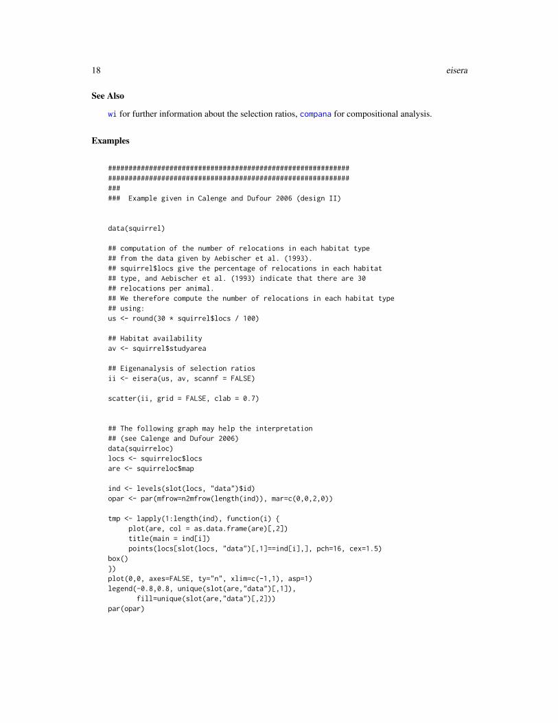
############################################################################################################################ Example given in Calenge and Dufour 2006 (design II)

data(squirrel)

## computation of the number of relocations in each habitat type## from the data given by Aebischer et al. (1993).## squirrel$locs give the percentage of relocations in each habitat## type, and Aebischer et al. (1993) indicate that there are 30## relocations per animal.## We therefore compute the number of relocations in each habitat type## using:us <- round(30 * squirrel$locs / 100)

## Habitat availabilityav <- squirrel$studyarea

## Eigenanalysis of selection ratiosii <- eisera(us, av, scannf = FALSE)

scatter(ii, grid = FALSE, clab = 0.7)

## The following graph may help the interpretation## (see Calenge and Dufour 2006)data(squirreloc)locs <- squirreloc$locsare <- squirreloc$map

ind <- levels(slot(locs, "data")$id)opar <- par(mfrow=n2mfrow(length(ind)), mar=c(0,0,2,0))

tmp <- lapply(1:length(ind), function(i) {plot(are, col = as.data.frame(are)[,2])title(main = ind[i])points(locs[slot(locs, "data")[,1]==ind[i],], pch=16, cex=1.5)

box()})plot(0,0, axes=FALSE, ty="n", xlim=c(-1,1), asp=1)legend(-0.8,0.8, unique(slot(are,"data")[,1]),

fill=unique(slot(are,"data")[,2]))par(opar)

enfa 19

############################################################################################################################ Example of design III

iii <- eisera(us, squirrel$mcp, scannf = FALSE)scatter(iii, grid = FALSE, clab = 0.7)

enfa Ecological Niche Factor Analysis

Description

enfa performs an Ecological Niche Factor Analysis. hist.enfa draws histograms of the row scoresor of the initial variables of the ENFA.

Usage

enfa(dudi, pr, scannf = TRUE, nf = 1)## S3 method for class 'enfa'hist(x, scores = TRUE, type = c("h", "l"), adjust = 1,

Acol, Ucol, Aborder, Uborder, Alwd = 1, Ulwd = 1, ...)

Arguments

dudi a duality diagram, object of class dudi (see Details)



nf an integer indicating the number of kept specialization axes

x an object of class enfa

scores logical. If TRUE, the histograms display the row scores of the ENFA. If FALSE,they display the niche on the environmental variables (in this case, this is equiv-alent to histniche)

type what type of plot should be drawn. Possible types are:"h" for histograms,"l" for kernel density estimates (see ?density).By default, type = "h" is used. If type = "l" is used, the position of the meanof each distribution is indicated by dotted lines

adjust if type = "l", a parameter used to control the bandwidth of the density estimates(see ?density)

Acol if type = "h", a color to be used to fill the histogram of the available pixels. iftype = "l", a color to be used for the kernel density estimates of the availablepixels

20 enfa

Ucol if type = "h", a color to be used to fill the histogram of the used pixels. if type= "l", a color to be used for the kernel density estimates of the used pixels

Aborder color for the border of the histograms of the available pixels

Uborder color for the border of the histograms of the used pixels

Alwd if type = "l", the line width of the kernel density estimates of the availablepixels

Ulwd if type = "l", the line width of the kernel density estimates of the used pixels


Details

The niche concept, as defined by Hutchinson (1957), considers the ecological niche of a species asan hypervolume in the multidimensional space defined by environmental variables, within whichthe populations of a species can persist. The Ecological Niche Factor Analysis (ENFA) has beendevelopped by Hirzel et al. (2002) to analyse the position of the niche in the ecological space.Nicolas Perrin (1984) described the position of the niche in the n-dimensional space using twomeasures: the M-specialization (hereafter termed marginality) and the S-specialization (hereaftertermed specialization). The marginality represents the squared distance of the niche barycentrefrom the mean available habitat. A large specialization corresponds to a narrow niche relative to thehabitat conditions available to the species.

The ENFA first extracts an axis of marginality (vector from the average of available habitat condi-tions to the average used habitat conditions). Then the analysis extracts successives orthogonal axes(i.e. uncorrelated), which maximises the specialization of the species. The calculations used in thefunction are described in Hirzel et al. (2002).

The function enfa can be used on both quantitative variables and qualitative variables (though theinterpretation of the results of the ENFA for qualitative variables is still under research), providedthat the table containing the values of habitat variables (columns) for each resource unit (rows) iscorrectly transformed (e.g. column-centered and standardised for tables containing only quantita-tive variables), and that appropriate column weights are given (e.g. the sum of the weights for thelevels of a factor should be the same as the weight of one quantitative variable). Therefore, the func-tion enfa requires that a preliminary multivariate analysis is performed on the table (using analysisof the family of duality diagram, e.g. principal component analysis or Hill and Smith analysis). Theobject returned by this preliminary analysis contains the appropriate weights and transformation ofthe original data frame. For example, the function dudi.mix can be used first on the data.framecontaining the value of both quantitative (e.g. slope, elevation) and qualitative habitat variables(e.g. vegetation) for each pixel of a raster map. The result of this analysis can then be passed asargument to the function enfa (see examples below).

Value

enfa returns a list of class enfa containing the following components:

call original call.

tab a data frame with n rows and p columns.


enfa 21

nf the number of kept specialization axes.

m the marginality (squared length of the marginality vector).

s a vector with all the eigenvalues of the analysis.

lw row weights, a vector with n components.

li row coordinates, data frame with n rows and nf columns.

cw column weights, a vector with p components.

co column coordinates, data frame with p rows and nf columns.

mar coordinates of the marginality vector.

Author(s)


References

Hutchinson, G.E. (1957) Concluding Remarks. Cold Spring Harbor Symposium on QuantitativeBiology, 22: 415–427.

Perrin, N. (1984) Contribution a l’ecologie du genre Cepaea (Gastropoda) : Approche descriptiveet experimentale de l’habitat et de la niche ecologique. These de Doctorat. Universite de Lausanne,Lausanne.

Hirzel, A.H., Hausser, J., Chessel, D. and Perrin, N. (2002) Ecological-niche factor analysis: Howto compute habitat-suitability maps without absence data? Ecology, 83, 2027–2036.

Basille, M., Calenge, C., Marboutin, E., Andersen, R. and Gaillard, J.M. (2008) Assessing habitatselection using multivariate statistics: Some refinements of the ecological-niche factor analysis.Ecological Modelling, 211, 233–240.

See Also

niche, kselect for other types of analysis of the niche, when several species are under studies,and scatter.enfa to have a graphical display of objects of class enfa. See madifa for anotherfactorial analysis of the ecological niche.

Examples

data(lynxjura)

map <- lynxjura$map

## We keep only "wild" indices.locs <- lynxjura$locslocs <- locs[slot(locs, "data")[,2]!="D",]

hist(map, type = "l")## The variable artif is far from symetric

## We perform a square root transformation

22 engen2008II

## of this variable## We therefore normalize the variable 'artif'slot(map,"data")[,4] <- sqrt(slot(map,"data")[,4])hist(map, type = "l")

## We prepare the data for the ENFAtab <- slot(map, "data")pr <- slot(count.points(locs, map), "data")[,1]

## We then perform the PCA before the ENFApc <- dudi.pca(tab, scannf = FALSE)

## The object 'pc' contains the transformed table (i.e.## centered so that all columns have a mean of 0## and scaled so that all columns have a variance of 1## 'pc' also contains the weights of the habitat variables,## and the weights of the pixels in the analysis

(enfa1 <- enfa(pc, pr,scannf = FALSE))

hist(enfa1)hist(enfa1, scores = FALSE, type = "l")

## scatterplotscatter(enfa1)

## randomization test## Not run:(renfa <- randtest(enfa1))plot(renfa)

## End(Not run)

engen2008II Measuring Habitat Selection Using the Method of Engen et al. (2008)

Description

These functions implements the method described by Engen et al. to measure the preference ofanimals for habitat variables in habitat selection studies.

Usage

engen2008II(us, av, id, nsim = 500, nsimra = 500)

engen2008I(us, av, nsimra=500)

engen2008II 23

## S3 method for class 'engenetalI'print(x, ...)

## S3 method for class 'engenetalII'print(x, ...)

Arguments

us a data frame containing the value of numeric habitat variables (columns) in eachsite (rows) used by the animals.

av a data frame containing the value of numeric habitat variables (columns) in eachsite (rows) available to the animals.

id a factor with as many elements as there are rows in us, indicating the ID of theanimal that used the corresponding rows in us.

nsim the number of randomizations used in the calculation of the total variance.

nsimra the number of random allocation of ranks used in the calculation of the normalscore (see details).

x an object of class engenetalI or engenetalII

... additional arguments to be passed to other functions (currently unused)

Details

Engen et al. (2008) proposed an original approach to measure the preference of animals for valuesof each particular variable of a multivariate set of environmental variables. Their approach wasoriginally developed for the case where there is a sample of used site is for each animal in a sampleof identified animals (e.g. using radiotelemetry or GPS), with several sites per animal (i.e., design IIaccording to the classification of Thomas and Taylor, 1990). However, we extended this approachto also include the case where habitat use is described by a sample of used site, with one site perunidentified animal (i.e., design I).

The original approach is the following: first, a normal score transformation of each habitat variableis performed: for each variable, the empirical cumulative distribution is computed, by dividing therank of the value of each available site by the number of observations. Note that the ties are rankedrandomly. Then, the inverse of the standard normal integral (see ?qnorm) of the cumulative distri-bution function is computed for all available sites: this results into a perfectly normal distributionof the habitat variables for the available sites. Then, the value of the cumulative distribution – es-timated from the available sites – is computed for each used site. Then, the inverse of the standardnormal integral is computed for each one.

Engen et al. (2008) suppose the following model describing how habitat use results from habitatavailability. Let

Zij

be the value of a given habitat variable (transformed according to the normal score) for the j-th siteused by the i-th animal. Then this value can be described by the model:

Zij = µ+ Ui + Vij

24 engen2008II

whereµ

is the preference for the habitat variable (0 indicates a non-preference),

Ui

andVij

are normal distributions with means equal to zero and variances equal to

σ2

andτ2

respectively. Engen et al. give fomula for the estimation of these parameters. Their estimation isdone by first estimating the total variance

σ2 + τ2

(this variance is estimated by sampling randomly one observation per animal – the parameter nsimcontrols the number of samples used in this computation; see Engen et al. 2008). Note that thecorrelation between the value observed for two used units sampled from all the units used by agiven animal is

ρ = σ2/(σ2 + τ2)

. A large value of rho indicates a large variation in the habitat used between animals (or a smallwithin-animal variation). The main parameter of concern is here the preference. The functionengen2008II allows to estimate these parameters.

The function engen2008I extends this model for design I studies (a sample of used sites and asample of available sites, animals not identified), by considering the following model for thesestudies:

Zij = µ+ Vij

whereµ

is the preference for the habitat variable (0 indicates a non-preference), and

Vij

are normal distributions with means equal to zero and variances equal to

σ2

.

Note that the habitat variables may be correlated on the study area. In this case, observed preferencefor a given variable may be an artefact of other variables prefered by animals. Supposing that thedata.frame containing the

Zij

engen2008II 25

’s is a realization of a multivariate normal distribution, we can compute, for each habitat variableand each used site, the *conditional* mean

mij

and *conditional* standard deviation

sij

of this variable at this site, *given* the values of the other habitat variables at this site (this is doneusing the algorithm described by Ripley, 1987, p.98). We then compute the standardized values

Pij = (Zij −mij)/sij

. The preference is then computed using these standardized values.

Because there may be ties in the distribution of values of habitat variables, the results may varydepending on the random order chosen for ties when computing the normal scores. Engen et al.recommended to repeat the function a large number of times, and to use the mean values as estimatesof the parameters. This is what the function does, and the number of randomization is controlled bythe parameter nsimra.

Note that all these methods rely on the following hypotheses: (i) independence between animals, (ii)independence between sites, and (iii) all animals are selecting habitat in the same way (in additionto "traditional" hypotheses in these kinds of studies: no territoriality, all animals having equal accessto all available resource units, etc., see Manly et al. 2002 for further details).

That the examples below provide an illustration and discussion of interesting and (at first sight)surprising properties of this method.

Value

engen2008I returns a list of class engenetalI, and engen2008II returns a list of class engenetalII.Both types of list contain two elements:

raw this is a list containing one data frame per habitat variable, containing the valueof the correlation rho (for engenetalII objects), mean preferences and standarderror of these preferences (columns) for each randomization performed (rows);

results a data frame containing the mean values over all the randomizations, of theseparameters (columns) for each habitat variable (rows).

Note

Be patient! these functions can be very long (depending on the number of sites and on the value ofsimra)

Author(s)


26 engen2008II

References

Engen, S., Grotan, V., Halley, D. and Nygard, T. (2008) An efficient multivariate approach forestimating preference when individual observations are dependent. Journal of Animal Ecology, 77:958–965.

Thomas, D. and Taylor, E. (1990) Study designs and tests for comparing resource use and availabil-ity. Journal of Wildlife Management, 54, 322–330.

Ripley, B. (1987) Stochastic Simulation. John Wiley and Sons.

See Also

niche, madifa, gnesfa for another approach to tackle the study of habitat selection. For categoricalvariables, see kselect

Examples

## Not run:

###################################################################################################

## Practical use of engen2008II

data(puechabonsp)map <- puechabonsp$map

## Removes the aspect (no factor allowed in the function)slot(map,"data")$Aspect <- NULL

## engen2008II:avail <- slot(map, "data")use <- join(puechabonsp$relocs, map)id <- slot(puechabonsp$relocs, "data")$Name

## This function can be very long:engen2008II(use, avail, id, nsimra=10)

## Practical use of engen2008I

data(lynxjura)ma <- lynxjura$maplo <- lynxjura$locsav <- slot(ma, "data")us <- join(lo, ma)us <- us[!is.na(us[,1]),]

## Idem, be patient here:

engen2008II 27

engen2008I(us, av, nsimra=10)

####################################################################################################### For a deeper discussion on## this method... a simulation:

##################################### First, simulation of a dataset## copy and paste this part into R,## but skip the reading of the## comments if you are not interested## into this simulation

## simulate the available points

suppressWarnings(RNGversion("3.5.0"))set.seed(235)av <- cbind(rnorm(1000, mean=0, sd=3), rnorm(1000, mean=0, sd=0.5))tt <- cbind(c(cos(-pi/4),sin(-pi/4)),c(cos(pi/4), sin(pi/4)))av <- as.data.frame(as.matrix(av)%*%tt)

## simulate the used points: we simulate a selection on the first## principal component of the PCA of the data.frame describing the## availability. In other words, we simulate the case where the## habitat selection occurs on the "common part" of the two habitat## variable (no preference for one particular variable).

us <- do.call("rbind", lapply(1:5, function(i) {us1 <- cbind(rnorm(30, mean=rnorm(1, -4, 1), sd=0.5),

rnorm(30, mean=rnorm(1, 0, 0.5), sd=0.2))

return(us1%*%tt)}))colnames(us) <- colnames(av) <- c("var1", "var2")id <- gl(5,30)

##################################### Study of the habitat selection on these data## The data are:## - us: a matrix containing the used sites for two## habitat variables## - av: a matrix containing the available sites for two

28 gnesfa

## habitat variables## - id: a vector containing the id of 5 animals

## First illustrate the use and availability of the two variables:

plot(av, xlab="Habitat variable 1", ylab="Habitat variable 2",col="grey", pch=16)

lius <- split(as.data.frame(us), id)junk <- lapply(1:5, function(i) points(lius[[i]], pch=16, col=i))

## -----> ***It is very clear that there is a selection***:## the animals select the low values of both habitat variables.## (this is what we actually simulated)

## Now perform the method of Engen et al. (2008):engen2008II(us, av, id)

## Surprisingly, the method seems to fail to identify the clear## habitat selection identified graphically...#### In fact, it does not fail:## this method identifies the part of habitat selection that is clearly## attributable to a given variable. Here the animals select the## the common factor expressed in the two variables, and it is impossible## to identify whether the selection is due only to the variable 1 or to## the variable 2: it is caused by both variable simultaneously.## Once the selection on the variable 2 (including the common part)## has been removed, there is no longer appearant selection on## variable 1. Once the selection caused by the variable 1## (including the common part) has been removed, there is no## longer selection on variable 2...#### For this reason, Engen et al. recommended to use this method## concurrently with other factor analyses of the habitat selection## such as madifa, kselect, niche (in ade4 package), etc.#### Note also the strong correlation between the value of two random## points used by a given animal. This indicates a strong variability## among animals...

## End(Not run)

gnesfa General Niche-Environment System Factor Analysis

gnesfa 29

Description

The function gnesfa allows to perform a general niche-environment system factor analysis.

Usage

gnesfa(dudi, Focus, Reference,centering = c("single", "twice"),scannf = TRUE, nfFirst = 2, nfLast = 0)

## S3 method for class 'gnesfa'print(x, ...)

Arguments

dudi an object of class dudi

Focus a vector containing the focus weights

Reference a vector containing the reference weights

centering a character string indicating the type of centering (see details)

scannf a logical value indicating whether the eigenvalues bar plot should be displayed

nfFirst the number of first axes to be kept

nfLast the number of last axes to be kept

x an object of class GNESFA

... further arguments to be passed to other functions

Details

The GNESFA is an algorithm which generalises several factor analyses of the ecological niche. Atable X gives the values of P environmental variables in N resource units (e.g. the pixels of a rastermap). A distribution of weights D describes the availability of the resource units to the species(if not specified, these weights are considered to be uniform). Another distribution of weights Dpdescribes the use of the resource units by the species (for example the proportion of relocations ineach pixel of a raster map).

Each environmental variable defines a dimension in a multidimensional space, the ecological space.The N resource units define a cloud of points in this space. Each point is associated to two weights.The GNESFA finds, in the ecological space, the directions on which these two distributions ofweights are the most different.

The GNESFA relies on a choice of the analyst, followed by three steps. Before all, the analysthas to choose one distribution of weights as the Reference distribution, and the other one as theFocus distribution; (i) The first table X is centred on the centroid of the Reference distribution;(ii) a principal component analysis of this Reference distribution is performed; (iii) the cloud ofpoints is distorted, so that the Reference distribution takes a standard spherical shape; (iv) a noncentred principal component analysis of the Focus distribution allows to identify the directions ofthe ecological space where the two distributions are the most different.

Depending on the distribution chosen as Reference, this algorithm returns results with differentmeanings (see examples). This algorithm is closely related to several common analyses of habitat

30 gnesfa

selection/niche (ENFA, MADIFA, Mahalanobis distances, selection ratios, etc.). The examplesbelow give some examples of the mathematical properties of this algorithm.

Note that the function takes a parameter named centering. Indeed, two types of centering can beperformed prior to the GNESFA. The choice "single" consists in the centering of the cloud of pointin the ecological space on the centroid of the Reference distribution. The choice "twice" consist tocenter the cloud of points on both the centroid of the Reference distribution and the centroid of theFocus distribution. This is done by projecting the cloud of points on the hyperplane orthogonal tothe marginality vector (the vector connecting the two centroids. If this choice is done, the GNESFAis identical to the commonly used Ecological Niche Factor Analysis (see examples).

Value

gnesfa returns a list of class gnesfa containing the following components:

call original call.

centering The type of centering required.


Reference a vector of length n containing the Reference weights.

Focus a vector of length n containing the Focus weights.

nfFirst the number of kept first axes.

nfLast the number of kept last axes.



l1 row normed coordinates, data frame with n rows and nf columns.

co column scores, data frame with p rows and nf columns.

cor the correlation between the GNESFA axes and the original variables

Author(s)


References

Calenge, C. and Basille, M. (2008) A General Framework for the Statistical Exploration of theEcological Niche. Journal of Theoretical Biology, 252: 674-685.

Calenge, C., Darmon, G., Basille, M., Loison, A. and Jullien, J.M. (2008) The factorial decompo-sition of the Mahalanobis distances in habitat selection studies. Ecology, 89, 555-566.

See Also

madifa, mahasuhab, enfa, wi for closely related methods (see Examples)

gnesfa 31

Examples

## Not run:

#################################################################### Study of the habitat selection by the chamois in the French## mountains of Les Bauges

## Loads the datadata(bauges)names(bauges)map <- bauges$maplocs <- bauges$locs

## displays the datamimage(map)image(map,1)points(locs, pch = 3)

## Prepares the data for the GNESFA:tab <- slot(map, "data")Dp <- slot(count.points(locs,map), "data")[,1]pc <- dudi.pca(tab, scannf = FALSE)

## Example of use with Dp = Referencegn <- gnesfa(pc, Reference = Dp, scannf=FALSE)

## One main axis:barplot(gn$eig)

## The correlation with variables indicate that## the elevation, the proximity to grass and to## deciduous forests:s.arrow(gn$cor)

## The factorial map of the niche...scatterniche(gn$li, Dp, pts = TRUE)

## The chamois is rather located at high elevation,## in the grass, far from deciduous forests

######################################################################################################################

32 gnesfa

#### Some interesting properties of the GNESFA########################################################################################################################

#################################################################### Interesting properties of the## choice: Dp as Reference## identical to the MADIFA## (Calenge et al. 2008),## See the help page of the function madifa## for other properties)

gn <- gnesfa(pc, Reference = Dp, scannf=FALSE,nfFirst = 7)

gn

## This is the same as the MADIFA:mad <- madifa(pc, Dp, scannf=FALSE)

## Indeed:plot(gn$li[,1], mad$li[,1])cor(gn$li[,1], mad$li[,1])

## And consequently the sum of the squared scores,## On the axes of the GNESFA...su <- apply(gn$l1,1,function(x) sum(x^2))

## ... is equal to the Mahalanobis distances between## the points and the centroid of the niche## (Clark et al. 1993, see the help page of mahasuhab)

su2 <- slot(mahasuhab(map, locs), "data")[,1]

## Indeed:all(su - su2 < 1e-7)plot(su, su2)

##################################################################

gnesfa 33

## Centering twice is identical to## the ENFA (Hirzel et al. 2002, see the help## page of the function enfa)...

########### ... If Dp is the Reference:

gn <- gnesfa(pc, Reference = Dp, center = "twice", scannf = FALSE)gn

enf <- enfa(pc, Dp, scannf = FALSE)plot(enf$li[,2], gn$li[,1])cor(enf$li[,2], gn$li[,1])

## The first specialization axis of the ENFA## is the first axis of the GNESFA!

########### ... If Dp is the Focus:

gn <- gnesfa(pc, Focus = Dp, center = "twice",scannf = FALSE, nfFirst = 6)

plot(enf$li[,2], gn$li[,6])cor(enf$li[,2], gn$li[,6])

## The first specialization axis of the ENFA## is the last axis of the GNESFA!

########### Whatever the distribution chosen as Reference,## projecting the cloud of points on the hyperplane## orthogonal to the marginality axis, and performing## a GNESFA in this subspace is identical to an ENFA!

## The marginality axis of the ENFA is identical## to the component "projmar" of the GNESFA

plot(enf$li[,1],gn$projmar)cor(enf$li[,1],gn$projmar)

##################################################################

34 histniche

## Interesting properties of the## case: Dp as Focus, one categorical## variable. Relationships with the selection## ratios of Manly et al. (1972, see the## help page of wi)

## For example, take the Elevation, and## define a factor with 4 levelselev <- data.frame(el = cut(slot(map, "data")$Elevation, 4))

## Now, compute the complete disjonctive tabledis <- acm.disjonctif(elev)head(dis)

## Now perform the GNESFA with Dp as Focus:pc <- dudi.pca(dis, scannf = FALSE)gn <- gnesfa(pc, Dp, scannf = FALSE, nfFirst = 3)

########### This analysis is closely related to the concept of## selection ratios

## Compute the percentage of use of each level:us <- apply(dis, 2, function(x) sum(x*Dp)/sum(Dp))av <- apply(dis, 2, function(x) sum(x)/length(x))

## The selection ratioswi <- widesI(us, av)$wi

## Compute the sum of the eigenvaluesum(gn$eig)

## Compute the sum of the selection ratios - 1sum(wi) - 1

## In other words, when the GNESFA (Dp as Focus) is## applied on only one categorical variable, this## analysis finds a set of axes which partition the## sum of the selection ratios so that it is maximum## on the first axes!!

## End(Not run)

histniche Histograms of the Ecological Niche

histniche 35

Description

histniche draws histograms of the niche-environment system: an histogram of the available re-source units (environment) is drawn on the same graph as an histogram of the used resource units(i.e. the niche), for comparison.

Usage

histniche(x, pr, type = c("h", "l"), adjust = 1,Acol, Ucol, Aborder, Uborder, Alwd = 1,Ulwd = 1, ylim, ncla = 15, ...)

Arguments

x a data frame giving the value of environmental variables (columns) in resourceunits (rows, e.g. the pixels of a raster map)

pr a vector of integers with the same length as nrow(x) (giving for example thenumber of detections in the pixels)

type what type of plot should be drawn. Possible types are:* "h" for histograms,* "l" for kernel density estimates (see ?density).By default, type = "h" is used. If type = "l" is used, the position of the meanof each distribution is indicated by dotted lines

adjust if type = "l", a parameter used to control the bandwidth of the density estimate(see ?density)

Acol color for the histograms of the available pixels

Ucol color for the histograms of the used pixels

Aborder if type = "h", color for the border of the histograms of the available pixels (seehelp(hist.default))

Uborder if type = "h", color for the border of the histograms of the used pixels (seehelp(hist.default))

Alwd if type = "l", line width for the density estimate of the available pixels

Ulwd if type = "l", line width for the density estimate of the used pixels

ylim the limits for the y axis

ncla The number of classes of the histogram


Author(s)


Examples

## Not run:

data(puechabonsp)

36 kselect

cp <- count.points(puechabonsp$relocs, puechabonsp$map)puechabonsp$map

histniche(slot(puechabonsp$map, "data"), slot(cp, "data")[,1])histniche(slot(puechabonsp$map, "data"), slot(cp, "data")[,1],

ty="l")

## End(Not run)

kselect K-Select Analysis: a Method to Analyse the Habitat Selection by Ani-mals

Description

Performs a multivariate analysis of ecological data (K-select analysis).

Usage

kselect(dudi, factor, weight, scannf = TRUE, nf = 2, ewa = FALSE)## S3 method for class 'kselect'print(x, ...)## S3 method for class 'kselect'kplot(object, xax = 1, yax = 2, csub = 2, possub = c("topleft",

"bottomleft", "bottomright", "topright"),addval = TRUE, cpoint = 1, csize = 1, clegend = 2, ...)

## S3 method for class 'kselect'hist(x, xax = 1, mar=c(0.1,0.1,0.1,0.1),

ncell=TRUE, csub=2,possub=c("bottomleft", "topleft",

"bottomright", "topright"),ncla=15, ...)

## S3 method for class 'kselect'plot(x, xax = 1, yax = 2, ...)prepksel(sa, hr, locs)

Arguments

dudi an object of class dudi

factor a factor with the same length as nrow(dudi$tab)

weight a numeric vector of integer values giving the weight associated to the rows ofdudi$tab

scannf logical. Whether the eigenvalues bar plot should be displayed

nf if scannf = FALSE, an integer indicating the number of kept axes

kselect 37

ewa logical. If TRUE, uniform weights are given to all animals in the analysis. IfFALSE, animal weights are given by the proportion of relocations of each animal(i.e. an animal with 10 relocations has a weight 10 times lower than an animalwith 100 relocations)

x, object an object of class kselect



addval logical. If TRUE, the frequency of the relocations per animal is displayed (seeexamples)

cpoint the size of the points (if 0, the points where no relocations are found are notdisplayed)

mar the margin parameter (see help(par))

ncell logical. If TRUE, the histogram shows the distribution of the cells of the rastermap where at least one relocation is found. If FALSE, the histogram shows thedistribution of the relocations

csub the character size for the legend, used with par("cex")*csub

csize the size coefficient for the points

clegend the character size for the legend used by par("cex")*clegend

possub a character string indicating the sub-title position ("topleft","topright","bottomleft","bottomright")

ncla the number of classes of the histograms

sa an object of class SpatialPixelsDataFrame containing the values of the envi-ronmental variables on the study area

hr an object of class SpatialPixelsDataFrame with the same number of rows assa, for which the pixels contain 1 inside the home ranges of the animals (oneanimal per column) and NA otherwise

locs an object of class SpatialPixelsDataFrame with the same dimensions as hr,containing the number of relocations of the animals (columns) in each pixel ofsa (rows)

... additional arguments to be passed to the generic function histniche, print or,in the case of plot.kselect, s.distri

Details

The K-select analysis is intended for hindcasting studies of habitat selection by animals using radio-tracking data. Each habitat variable defines one dimension in the ecological space. For each animal,the difference between the vector of average available habitat conditions and the vector of averageused conditions defines the marginality vector. Its size is proportional to the importance of habitatselection, and its direction indicates which variables are selected. By performing a non-centeredprincipal component analysis of the table containing the coordinates of the marginality vectors ofeach animal (row) on the habitat variables (column), the K-select analysis returns a linear combina-tion of habitat variables for which the average marginality is greatest. It is a synthesis of variableswhich contributes the most to the habitat selection. As with principal component analysis, thebiological significance of the factorial axes is deduced from the loading of variables.

prepksel allows to prepare the data for the kselect analysis (see examples).

38 kselect

plot.kselect returns a summary of the analysis: it displays (i) a graph of the correlations betweenthe principal axes of the PCA of the objects of class dudi passed as argument and the factorial axesof the K-select analysis; (ii) a graph giving the scores of the habitat variables on the factorial axes ofthe K-select analysis; (iii) the barplot of the eigenvalues of the analysis (each eigenvalue measure themean marginality explained by the axis; (iv) the projection of the non-recentred marginality vectorson the factorial plane (the origin of the arrow indicates the average available habitat conditions,and the end of the arrow indicates the average used conditions); (v) the projection of the resourceunits available to each animal on the first factorial plane and (vi) the coordinates of the recentredmarginality vectors (i.e. recentred so that they have a common origin) on the first factorial plane.

kplot.kselect returns one graph per animal showing the projections of the available resourceunits on the factorial plane, as well as their use by the animal. hist.kselect does the same thing,but on one dimension instead of two.

Value

kselect returns a list of the class kselect and dudi (see dudi).

Author(s)


References

Calenge, C., Dufour, A.B. and Maillard, D. (2005) K-select analysis: a new method to analysehabitat selection in radio-tracking studies. Ecological modelling, 186, 143–153.

See Also

s.distri, and dudi for class dudi.

Examples

## Not run:## Load the datadata(puechabonsp)

locs <- puechabonsp$relocsmap <- puechabonsp$map

## compute the home range of animals (e.g. using the minimum convex## polygon)pc <- mcp(locs[,"Name"])

## rasterize ithr <- hr.rast(pc, map)

## Compute the number of relocation in each pixel of the mapcp <- count.points(locs[,"Name"], map)

madifa 39

## prepares the data for the kselect analysisx <- prepksel(map, hr, cp)tab <- x$tab

## Example of analysis with two variables: the slope and the elevation.## Have a look at the use and availability of the two variables## for the 4 animalstab <- tab[,((names(tab) == "Slope")|(names(tab) == "Elevation"))]tab <- scale(tab)tmp <- split.data.frame(tab, x$factor)wg <- split(x$weight, x$factor)opar <- par(mfrow = n2mfrow(nlevels(x$factor)))for (i in names(tmp))

s.distri(scale(tmp[[i]]), wg[[i]])par(opar)

## We call a new graphic windowx11()## A K-select analysisacp <- dudi.pca(tab, scannf = FALSE, nf = 2)kn <- kselect(acp, x$factor, x$weight,scannf = FALSE, nf = 2)

# use of the generic function scatterscatter(kn)

# Displays the first factorial planekplot(kn)kplot(kn, cellipse = 0, cpoint = 0)kplot(kn, addval = FALSE, cstar = 0)

# this factorial plane can be compared with# the other graph to see the rotation proposed by# the analysisgraphics.off()

# Displays the first factorial axishist(kn)

# Displays the second factorial axishist(kn, xax = 2)

# Summary of the analysisplot(kn)

## End(Not run)

madifa The MADIFA: a Factorial Decomposition of the Mahalanobis Dis-tances

40 madifa

Description

The MADIFA allows a factorial decomposition of the Mahalanobis distances. This method is pre-sented here in the framework of niche-environment studies.

predict.madifa allows the computation of the Mahalanobis Distances based on a restricted num-ber of factorial axes.All other functions allow various graphical displays of the results of the MADIFA.

Usage

madifa(dudi, pr, scannf = TRUE, nf = 2)## S3 method for class 'madifa'print(x, ...)## S3 method for class 'madifa'scatter(x, xax = 1, yax = 2, pts = FALSE, percent = 95,

clabel = 1, side = c("top", "bottom", "none"),Adensity, Udensity, Aangle, Uangle, Aborder,Uborder, Acol, Ucol, Alty,Ulty, Abg, Ubg, Ainch, Uinch, ...)

## S3 method for class 'madifa'hist(x, scores = TRUE, type = c("h", "l"), adjust = 1, Acol,

Ucol, Aborder, Uborder, Alwd = 1, Ulwd = 1, ...)## S3 method for class 'madifa'predict(object, map, nf, ...)s.madifa(x, xax = 1, yax = 2, cgrid = 1, clab = 1, ...)## S3 method for class 'madifa'plot(x, map, xax = 1, yax = 2, cont = FALSE, ...)

Arguments

dudi a duality diagram, an object of class dudi



nf an integer indicating the number of kept factorial axes

x,object an object of class madifa



pts logical. Whether the points should be drawn. If FALSE, minimum convex poly-gons are displayed

percent 100 minus the proportion of outliers to be excluded from the computation of theminimum convex polygons

clabel a character size for the columns

side if "top", the legend of the kept axis is upside, if "bottom" it is downside, if"none" no legend

Adensity the density of shading lines, in lines per inch, for the available pixels polygon.See polygon for more details

madifa 41

Udensity the density of shading lines, in lines per inch, for the used pixels polygon. Seepolygon for more details

Aangle the slope of shading lines, given as an angle in degrees (counter-clockwise), forthe available pixels polygon

Uangle the slope of shading lines, given as an angle in degrees (counter-clockwise), forthe used pixels polygon

Aborder the color for drawing the border of the available pixels polygon (or of the barsof the histogram) . See polygon for more details

Uborder the color for drawing the border of the used pixels polygon (or of the bars of thehistogram). See polygon for more details

Acol the color for filling the available pixels polygon. if pts == FALSE, the color forthe points corresponding to available pixels

Ucol the color for filling the used pixels polygon. if pts == FALSE, the color for thepoints corresponding to used pixels

Alty the line type for the available pixels polygon, as in par

Ulty the line type for the used pixels polygon, as in par

Abg if pts == TRUE, background color for open plot symbols of available pixels

Ubg if pts == TRUE, background color for open plot symbols of used pixels

Ainch if pts == TRUE, heigth in inches of the available pixels

Uinch if pts == TRUE, heigth in inches of the largest used pixels

scores logical. If TRUE, the histograms display the row scores of the MADIFA. IfFALSE, they display the niche on the environmental variables (in this case, thisis equivalent to histniche)

type what type of plot should be drawn. Possible types are:* "h" for histograms,* "l" for kernel density estimates (see ?density).By default, type = "h" is used. If type = "l" is used, the position of the meanof each distribution is indicated by dotted lines

adjust if type = "l", a parameter used to control the bandwidth of the density estimates(see ?density)

Alwd if type = "l", the line width of the kernel density estimates of the availablepixels

Ulwd if type = "l", the line width of the kernel density estimates of the used pixels

cgrid a character size, parameter used with par("cex")* cgrid to indicate the mesh ofthe grid

clab if not NULL, a character size for the labels, used with par("cex")*clab

map an object of class SpatialPixelsDataFrame

cont logical. Whether contour lines should be added to the maps

... additional arguments to be passed to the functions print, scatter, and plot

42 madifa

Details

The Mahalanobis distances are often used in the context of niche-environment studies (Clark etal. 1993, see the function mahasuhab). Each environmental variable defines a dimension in amultidimensionnal space, namely the ecological space. The Mahalanobis distance between anyresource unit in this space (e.g. the point defined by the values of environmental variables in a pixelof a raster map) and the centroid of the niche (the distribution of used resource units) can be usedto give a value of eccentricity to this point.

For a given distribution of available resource units, for which a measure of Mahalanobis distancesis desired, the MADIFA (MAhalanobis DIstances Factor Analysis) partitions the ecological spaceinto a set of axes, so that the first axes maximises the average proportion of their squared Maha-lanobis distances. Note that the sum of the squared scores of any resource unit on all the axesof the analysis is equal to the squared Mahalanobis distances for this resource unit. Thus, theMADIFA partitions the Mahalanobis distances into several axes of biological meaning (see exam-ples). predict.madifa allows to compute approximate Mahalanobis distances from the axes of theMADIFA.

plot.madifa returns a graphical summary of the analysis: it returns graphs of (i) the eigenval-ues of the analysis (each eigenvalue measures the average Mahalanobis distance explained by eachfactorial axis); (ii) the scores of the habitat variables (i.e. the coefficients associated to each envi-ronmental variable in the linear combination defining the axes) - note that as the ecological spaceis distorted to "sphericize" the niche, the factorial axes are no longer orthogonals, and the scores ofthe variables are distributed within an ellipsoid instead of an hypersphere of radius equal to one inclassical PCA. The limits of this ellipsoid is displayed on this graph, to see the amount of distortiondone by the analysis (further research needs yet to be done on this graph); (iii) The projection of theavailable and used points on the factorial plane of the MADIFA; (iv) The map of the Mahalanobisdistances computed from the original environmental variables; (v) the map of the approximatedMahalanobis distances computed from the two axes displayed in this plot; the correlations betweenthe original environmental variables and the factorial axes; (v) the map of the first factorial axis and(vi) the map of the second factorial axis.

hist.madifa returns a graph of the niche and the available resource units on the factorial axes ofthe analysis.

Value

madifa returns a list of class madifa containing the following components:

call original call.



nf the number of kept factorial axes.


lw row weights, a vector with n components.


l1 row normed coordinates, data frame with n rows and nf columns.

cw column weights, a vector with p components.

co column coordinates, data frame with p rows and nf columns.

madifa 43

mahasu a vector of length n containing the squared Mahalanobis distances for the n units.

cor the correlation between the MADIFA axes and the original variable

predict.madifa returns a matrix of class SpatialPixelsDataFrame.

Author(s)


References


Calenge, C., Darmon, G., Basille, M., Loison, A. and Jullien J.M. (2008) The factorial decomposi-tion of the Mahalanobis distances in habitat selection studies. Ecology, 89, 555–566.

See Also

mahasuhab for a detailed description of the Mahalanobis distances, enfa and gnesfa for closelyrelated methods.

Examples

## Not run:

data(bauges)

map <- bauges$maplocs <- bauges$loc

## We prepare the data for the MADIFAtab <- slot(map, "data")pr <- slot(count.points(locs, map), "data")[,1]

## We then perform the PCA before the MADIFApc <- dudi.pca(tab, scannf = FALSE)(mad <- madifa(pc, pr, nf=7,

scannf = FALSE))

########################################### #### Graphical exploration of the MADIFA #### ###########################################

hist(mad)

plot(mad, map)

## this plot represents:

44 madifa

## - the eigenvalues diagram## - the scores of the columns on the axes## - a graph of the niche in the available space## - a map of the Mahalanobis distances computed## using all environmental variables## - a map of the Mahalanobis distances computed## using the two factorial axes used in the## previous graphs## - the correlation between habitat variables## and factorial axes## - the geographical maps of the two## factorial axes

## predict with just the first axispred <- predict(mad, map, nf=1)image(pred)

########################################### #### Mathematical properties of MADIFA #### ###########################################

## mad$li is equal to mad$l1, up to a constant (mad$l1 is normed)plot(mad$li[,1],mad$l1[,1])

## This constant is the square root of the corresponding eigenvalue:## the variance of mad$l1 is equal to the eigenvalueapply(mad$l1,2,function(x) sum(x^2))/nrow(mad$li)

## the variance of mad$l1 weighted by pr is equal to 1apply(mad$l1,2,function(x) sum(mad$pr*x^2)/sum(mad$pr))

## Therefore, the eigenvalues are equal to the average of Mahalanobis## distance for the available resource units on each axismean(mahalanobis(matrix(mad$l1[,1], ncol=1), 0, 1))mad$eig[1]

## Computation of the Mahalanobis distancesma1 <- mahasuhab(map, locs)

## The sum of squared scores for a given Resource unit is equal to the## Mahalanobis distancesma2 <- apply(mad$l1,1, function(x) sum(x^2))plot(ma2, slot(ma1, "data")[,1])

## End(Not run)

mahasuhab 45

mahasuhab Habitat Suitability Mapping with Mahalanobis Distances.

Description

This function computes the habitat suitability map of an area for a species, given a set of locationsof the species occurences (Clark et al. 1993). This function is to be used in habitat selection studies,when animals are not identified.

Usage

mahasuhab(x, pts, type = c("distance", "probability"))

Arguments

x a raster map of class SpatialPixelsDataFrame

pts a data frame with two columns, giving the coordinates of the species locations

type a character string. Whether the raw "distance" should be returned, or ratherthe "probability" (see details).

Details

Let assume that a set of locations of the species on an area is available (gathered on transects, orduring the monitoring of the population, etc.). If we assume that the probability of detecting anindividual is independent from the habitat variables, then we can consider that the habitat found atthese sites reflects the habitat use by the animals.

The Mahalanobis distances method has become more and more popular during the past few yearsto derive habitat suitability maps. The niche of a species is defined as the probability density func-tion of presence of a species in the multidimensionnal space defined by the habitat variables. Ifthis function can be assumed to be multivariate normal, then the mean vector of this distributioncorresponds to the optimum for the species.

The function mahasuhab first computes this mean vector as well as the variance-covariance matrixof the niche density function, based on the value of habitat variables in the sample of locations.Then, the *squared* Mahalanobis distance from this optimum is computed for each pixel of themap. Thus, the smaller this squared distance is for a given pixel, and the better is the habitat in thispixel.

Assuming multivariate normality, squared Mahalanobis distances are approximately distributed asChi-square with n-1 degrees of freedom, where n equals the number of habitat characteristics. Ifthe argument type = "probability", maps of these p-values are returned by the function. As suchthese are the probabilities of a larger squared Mahalanobis distance than that observed when x issampled from the niche.

Value

Returns a raster map of class SpatialPixelsDataFrame.

46 niche.test

Note

The computation of the squared Mahalanobis distances inverts the variance-covariance matrix ofthe niche density function (see ?mahalanobis). It is therefore important that the habitat variablesconsidered are not too correlated among each other. When the habitat variables are too correlated,the variance-covariance matrix is singular and cannot be inverted.

Note also that it is recommended to scale the variables before the computation, so that they all havethe same variance, and therefore the same weight in the analysis (see examples below).

Author(s)


References


See Also

madifa and dunnfa for factor analyses of the Mahalanobis distances, domain for another methodof habitat suitability mapping, mahalanobis for information on the computation of Mahalanobisdistances.

Examples

## loads the datadata(lynxjura)ma <- lynxjura$maplo <- lynxjura$locs[,1:2]

## We first scale the mapsslot(ma, "data") <- dudi.pca(slot(ma, "data"), scannf=FALSE)$tab

## habitat suitability mappinghsm <- mahasuhab(ma, lo, type = "probability")image(hsm)title(main = "Habitat suitability map for the Lynx")points(lo, pch = 3)

niche.test Monte-Carlo Test on Parameters of the Ecological Niche

Description

niche.test tests for the significance of two parameters of the ecological niche of a species (marginal-ity and tolerance), using Monte-Carlo methods. This is a bivariate test.

niche.test 47

Usage

niche.test(x, pts, nrep = 999, o.include = TRUE, ...)

Arguments

x a raster map of class SpatialPixelsDataFrame

pts an object inheriting the class SpatialPoints

nrep the number of permutations

o.include logical, passed to biv.test. If TRUE, the origin is included in the plot

... further arguments passed to biv.test

Details

niche.test tests the significance of two parameters describing the ecological niche: the marginal-ity (squared length of the vector linking the average available habitat conditions to the average usedhabitat conditions in the ecological space defined by the habitat variables), and the tolerance (inertiaof the niche in the ecological space, i.e. the sum over all variables of the variance of used pixels).

At each step of the randomisation procedure, the test randomly allocates the n points in the pixelsof the map. The marginality and the tolerance are then recomputed on this randomised data set.

Actual values are compared to random values with the help of the function biv.test.

Value

Returns a list containing the following components:

dfxy a data frame with the randomized values of marginality (first column) and toler-ance (second column).

obs the actual value of marginality and tolerance.

Warning

biv.test uses the function kde2d of the package MASS.

Author(s)

Mathieu Basille <[email protected]>Clement Calenge <[email protected]>

See Also

biv.test for more details on bivariate tests. histniche for the histograms of the variables of theniche.

48 pheasant

Examples

## Not run:data(chamois)

niche <- niche.test(chamois$map,chamois$locs,side = "bottom")

names(niche)

## End(Not run)

pheasant Radio-Tracking of Pheasants

Description

This data set describes the use and availability of 5 habitat types for 13 pheasants monitored usingradio-tracking.

Usage

data(pheasant)

Format

This list has three components:

studyarea a data frame giving the proportion of each habitat type (columns) on the study area.These habitat types are Scrub, Broadleaf, Coniferous, Grassland and Crop. These propor-tions are repeated by rows, for all animals (rows)

mcp a data frame giving the proportion of each habitat type (columns) in the home range of eachanimal (rows)

locs a data frame giving the proportion of relocations of each animal (rows) reported in 3 of the5 habitat types (columns). Indeed, Coniferous and Crops were not used by most of theanimals.

Source


predict.enfa 49

predict.enfa Habitat Suitability Maps Built from the ENFA

Description

predict.enfa computes habitat suitability maps using the Ecological-Niche Factor Analysis andthe Mahalanobis distances method.

Usage

## S3 method for class 'enfa'predict(object, map, nf, ...)

Arguments

object an object of class enfa

map an object of class SpatialPixelsDataFrame.

nf the number of axes of specialization kept for the predictions. By default, all axeskept in object are used


Details

The predictions are based on the position of the niche defined by the ENFA within the multidimen-sional space of environmental variables. The ENFA produces row coordinates for each pixel, whichare used with the function mahalanobis. For each pixel, this function computes the Mahalanobisdistances from the barycentre of the niche.

Actually, the function predict.enfa is identical to the function mahasuhab, except that the habitatsuitability map is computed using the axes of the ENFA, instead of the raw data.

Note that the MADIFA allows a more consistent factorial decomposition of the Mahalanobis dis-tances.

Value

Returns a raster map of class SpatialPixelsDataFrame.

Author(s)


References


Hirzel, A.H., Hausser, J., Chessel, D. & Perrin, N. (2002) Ecological-niche factor analysis: How tocompute habitat-suitability maps without absence data? Ecology, 83, 2027–2036.

50 puech

See Also

mahalanobis for information on the computation of Mahalanobis distances. mahasuhab for moredetails on the computation of habitat suitability maps using the Mahalanobis distances. madifa fora more consistent factorial decomposition of the Mahalanobis distances

Examples

## Not run:data(lynxjura)

map <- lynxjura$map


pr <- slot(count.points(locs, map), "data")[,1]

(enfa1 <- enfa(dudi.pca(slot(map, "data"), scannf=FALSE),pr, scannf = FALSE))

## Compute the predictionpred <- predict(enfa1, map)image(pred)contour(pred, col="green", add=TRUE)points(locs, pch = 3)

## End(Not run)

puech Radio-Tracking Data of Wild Boar (2)

Description

This data set stores the results of the monitoring of 6 wild boar at Puechabon (Mediterranean habitat,South of France). These data have been collected by Daniel Maillard (Office national de la chasseet de la faune sauvage).

Usage

data(puech)

Details

The list puech has two components:

puech$relocations is an object of class SpatialPixelsDataFrame containing the relocations ofthe wild boar resting sites in summer. It contains the coordinates of the relocations and the name ofthe corresponding wild boar.

puechdesIII 51

puech$map is n object of class SpatialPixelsDataFrame that describe nine environmental vari-ables on the study area (the elevation, the tree cover, the shrub cover, the distance to recreationaltrails, the distance to crops, the distance to water points, the grass cover, the slope and the sunshine).

Note that both the maps and the relocations have been slightly "damaged" to preserve the copyrighton the data.

References

Maillard, D. (1996). Occupation et utilisation de la garrigue et du vignoble mediterraneens par leSanglier. Universite d’Aix-Marseille III: PhD thesis.

puechdesIII Habitat Selection by the Wild Boar at Puechabon

Description

This data set contains two data frames describing the use and the availability of 3 elevation classesfor 6 wild boars (Sus scrofa L.) monitored using radio-tracking at Puechabon (South of France).These data have been collected by Daniel Maillard (Office national de la chasse et de la faunesauvage).

Usage

data(puechdesIII)

Details

The list puechdesIII has two components:The data frame used describes the number of telemetry relocations for each of the 6 animals in eachof the three elevation classes.The data frame available describes a sample of random points placed in the areas available tothese wild boars (a buffer area of 200 m around the relocations).

Source

Maillard, D. (1996) Occupation et utilisation de la garrigue et du vignoble mediterraneens par leSanglier. Universite d’Aix-Marseille III: PhD thesis.

52 rand.kselect

rand.kselect Test of the Third-Order Habitat Selection

Description

rand.kselect tests whether the marginality vector of animals is significantly larger than what isexpected under the hypothesis of random habitat use (third-order habitat selection: selection by theanimals of the relocations within their home range; the habitat availability is measured for eachanimal). The effect of each variable on individual marginality is also tested. Finally, the pertinenceof a K-select analysis is also tested. This is a randomisation test. The alpha-level of the tests isajusted using the Bonferroni inequality.

Usage

rand.kselect(dudi, factor, weight, nrep = 200, alpha = 0.05, ewa = FALSE)## S3 method for class 'rand.kselect'print(x, ...)

Arguments

dudi an object of class dudi.factor a factor defining the animals identityweight a weight vector of integer values (number of relocations counted in each re-

source unit in row of the object dudi)nrep the number of repetitions of the testalpha the alpha level for the tests.ewa logical. If TRUE, uniform weights are given to all animals in the analysis. If

FALSE, animal weights are given by the proportion of relocations of each animal(i.e. an animal with 10 relocations has a weight 10 times lower than an animalwith 100 relocations)

x an object of the class rand.kselect.... further arguments to be passed to the generic function print

Details

This test is carried out by simulating a random use of space by animals. rand.kselect is closelyrelated to the function kselect (same arguments).

At each step of the randomisation procedure, and for each animal, the test randomly allocates thenk relocations (where nk is the sum of the weight vector for the animal k) in the Ik pixels availableto this animal (where Ik is the length of the weight vector for animal k).

The length of the marginality vector is recomputed at each step of the randomisation procedure andfor each animal. The effect of each variable on the use of pixels by each animal is measured by thecriterion "(average habitat variable j used by animal i) minus (average habitat variable j available toanimal i)". Finally the value of the first eigenvalue of the K-select analysis provides a criterion totest the pertinence of the K-select analysis.

All these values are then compared to the observed values to assess the significance of theses effects.

rand.kselect 53

Value

Returns an object of class rand.kselect. This list has three components:

global a vector of length 2 giving the results of the randomisation procedure for thefirst eigenvalue of the K-select analysis.

marg a matrix giving the significance of the marginality of each animal.

per.ind a list giving the results of the randomisation test for the coordinates of themarginality vector for each animal on each habitat variable.

alpha the alpha level of the tests.

Author(s)


References

Calenge, C., Dufour, A.B. and Maillard, D. (2005) K-select analysis: a new method to analysehabitat selection in radio-tracking studies. Ecological modelling, 186, 143–153.

See Also

kselect to perform a K-select analysis.

Examples

## Not run:## Loads the datadata(puechabonsp)

locs <- puechabonsp$relocsmap <- puechabonsp$map

## compute the home range of animals (e.g. using the minimum convex## polygon)pc <- mcp(locs[,"Name"])

## rasterize ithr <- do.call("data.frame", lapply(1:nrow(pc), function(i) {

overlay(map, geometry(pc[i,]))}))names(hr) <- slot(pc, "data")$idcoordinates(hr) <- coordinates(map)gridded(hr) <- TRUE

## Compute the number of relocation in each pixel of the mapcp <- count.points(locs[,"Name"], map)

## prepares the data for the kselect analysis

54 randtest.enfa

x <- prepksel(map, hr, cp)tab <- x$tabdud <- dudi.mix(tab, scannf = FALSE, nf = 2)

## the randomisation tests## be patient, this can be very long on some machines(te <- rand.kselect(dud, x$factor, x$weight, nrep = 500))

## End(Not run)

randtest.enfa Randomisation Test for the Ecological Niche Factor Analysis

Description

randtest.enfa performs a randomisation test for the Ecological Niche Factor analysis (ENFA).

Usage

## S3 method for class 'enfa'randtest(xtest, nrepet = 999, ...)

Arguments

xtest an object of class enfa

nrepet the number of iterations for the randomisation test

... further arguments to be passed to the generic function randtest

Details

This test is carried out by simulating a random distribution of the species occurrences in the pixelsof a map.

At each step of the randomisation procedure, the test randomly allocates the nk occurrences (wherenk is the sum of the occurrence vector pr of the object of class enfa) in the Ik pixels of the focusarea (where Ik is the length of this occurrence vector).

At each step of the procedure, the first eigenvalue of the ENFA performed on the randomised dataset is recomputed. This value provides a criterion to test the pertinence of the ENFA analysis.

Value

returns a list of class randtest

Author(s)


scatter.enfa 55

References

Manly, B.F.J. (1997) Randomization, Bootstrap and Monte Carlo Methods in Biology. London:Chapman & Hall.

Hirzel, A.H., Hausser, J., Chessel, D. and Perrin, N. (2002) Ecological-niche factor analysis: Howto compute habitat suitability maps without absence data? Ecology, 83, 2027–2036.

See Also

enfa

Examples

## Not run:data(chamois)locs <- chamois$locsmap <- chamois$map

## prepare the datatab <- slot(map, "data")tab$Vegetation <- NULLpr <- slot(count.points(locs, map), "data")[,1]

en <- enfa(dudi.pca(tab, scannf=FALSE), pr, scannf = FALSE)(tutu <- randtest(en, nrepet = 100))plot(tutu)

## End(Not run)

scatter.enfa Scatter Plot of the Results of the ENFA

Description

Performs the scatter diagrams of objects of class enfa.

Usage

## S3 method for class 'enfa'scatter(x, xax = 1, yax = 2, pts = FALSE, nc = TRUE,

percent = 95, clabel = 1, side = c("top", "bottom", "none"),Adensity, Udensity, Aangle, Uangle, Aborder, Uborder,Acol, Ucol, Alty, Ulty, Abg, Ubg, Ainch, Uinch, ...)

56 scatter.enfa

Arguments

x an object of class enfa




nc whether or not the niche center should be displayed








Aborder the color for drawing the border of the available pixels polygon. See polygonfor more details

Uborder the color for drawing the border of the used pixels polygon. See polygon formore details

Acol the color for filling the available pixels polygon. if pts == FALSE, the color forthe points corresponding to available pixels

Ucol the color for filling the used pixels polygon. if pts == FALSE, the color for thepoints corresponding to used pixels

Alty the line type for the available pixels polygon, as in par

Ulty the line type for the used pixels polygon, as in par

Abg if pts == TRUE, background color for open plot symbols of available pixels

Ubg if pts == TRUE, background color for open plot symbols of used pixels

Ainch if pts == TRUE, heigth in inches of the available pixels

Uinch if pts == TRUE, heigth in inches of the largest used pixels


Details

scatter.enfa displays a factorial map of pixels, as well as the projection of the vectors of thecanonical basis multiplied by a constant of rescaling. The kept axes for the plot are specified in acorner.

scatter.enfa 57

Author(s)


References

Basille, M., Calenge, C., Marboutin, E., Andersen, R. & Gaillard, J.M. (2008) Assessing habitatselection using multivariate statistics: Some refinements of the ecological-niche factor analysis.Ecological Modelling, 211, 233–240.

See Also

enfa, scatter

Examples

data(lynxjura)

map <- lynxjura$map


hist(map, type = "l")## The variable artif is far from symetric

## We perform a square root transformation## of this variable## We therefore normalize the variable 'artif'slot(map,"data")[,4] <- sqrt(slot(map,"data")[,4])hist(map, type = "l")

## We prepare the data for the ENFAtab <- slot(map, "data")pr <- slot(count.points(locs, map), "data")[,1]

## We then perform the PCA before the ENFApc <- dudi.pca(tab, scannf = FALSE)

## We perform the ENFA(enfa1 <- enfa(pc, pr, scannf = FALSE))

scatter(enfa1)

58 scatterniche

scatterniche Display the Niche in the Ecological Space

Description

scatterniche displays the niche in the Ecological space (multidimensional space defined by habi-tat variables).

Usage

scatterniche(x, pr, xax = 1, yax = 2, pts = FALSE,percent = 95, clabel = 1,side = c("top", "bottom", "none"),Adensity, Udensity, Aangle, Uangle, Aborder,Uborder, Acol, Ucol, Alty, Ulty, Abg,Ubg, Ainch, Uinch, ...)

Arguments

x a data frame giving the value of environmental variables (columns) in resourceunits (rows, e.g. the pixels of a raster map)

pr a vector giving the utilisation weight for each resource unit











Aborder the color to draw the border of the available pixels polygon. See polygon formore details

Uborder the color to draw the border of the used pixels polygon. See polygon for moredetails

squirrel 59

Acol the color for filling the available pixels polygon. if pts==FALSE, the color forthe points corresponding to available pixels

Ucol the color for filling the used pixels polygon. if pts==FALSE, the color for thepoints corresponding to used pixels

Alty the line type for the available pixels polygon, as in par.

Ulty the line type for the used pixels polygon, as in par.

Abg if pts==TRUE, background color for open plot symbols of available pixels

Ubg if pts==TRUE, background color for open plot symbols of used pixels

Ainch if pts==TRUE, heigth in inches of the available pixels

Uinch if pts==TRUE, heigth in inches of the largest used pixels


Author(s)

Mathieu Basille <[email protected]>Clement Calenge <[email protected]>

Examples

data(chamois)cpi <- slot(count.points(chamois$locs, chamois$map),"data")[,1]chamois$map

tab <- slot(chamois$map, "data")

## we focus on the distance to ecotone and on the slope,## after centring and scaling (with the help of a PCA)scatterniche(dudi.pca(tab[,2:3], scannf=FALSE)$tab, cpi)scatterniche(dudi.pca(tab[,2:3], scannf=FALSE)$tab, cpi, pts=TRUE)

squirrel Radio-Tracking Data of Squirrels

Description

This data set describes the use and availability of 5 habitat types for 17 squirrels monitored usingradio-tracking. See also the dataset squirreloc.

Usage

data(squirrel)

60 squirreloc

Format

This list has three components:

studyarea a data frame giving the proportion of each habitat type (columns) on the study area.These proportions are repeated by rows, for all animals

mcp a data frame giving the proportion of each habitat type (columns) in the home range of eachanimal (rows)

locs a data frame giving the proportion of relocations of each animal (rows) reported in eachhabitat type (columns).

Source


squirreloc Radio-tracking of squirrels

Description

This data set contains the trajectories of 15 radio-monitored squirrels, as well as the vector maps ofhabitat composition.

Usage

data(squirreloc)

Format

This data set is a list of two objects: locs is a SpatialPointsDataFrame containing the relocationsof 15 squirrels

map is an object of class SpatialPolygonsDataFrame containing the habitat composition of thearea. The habitat types and colour coding are stored in the data.frame

Details

The dataset squirreloc comes from the Ranges VI software. It has been used to illustrate thecompositional analysis (see ?compana) and the eigenanalysis of selection ratios (see ?eisera). Seealso the dataset squirrel.

Source

Kenward, R.E., South, A.B. and Walls, S.S. (2003). Ranges6 v1.2 : For the analysis of tracking andlocation data. Online manual. Anatrack Ltd. Wareham, UK. ISBN 0-9546327-0-2.

vanoise 61

vanoise Habitat Use by Three Species of Galliformes in the Vanoise NationalParc

Description

This data frame describes the habitat use by the Black Grouse (Tetrao tetrix), the Rock Partridge(Alectoris graeca) and the Rock Ptarmigan (Lagopus mutus), in the Vanoise National Park (FrenchAlps), from 1990 to 2000.

Usage

data(vanoise)

Format

This data frame has 3110 rows and eight columns describing the habitat composition for each oc-currence of three species of Galliformes. For each located occurrence (in rows), the employees ofthe national park have noted: the species, the elevation (in metres), the aspect (8 classes), the habitattype (7 categories, FR means "fallen rocks") and the date (season, day, month and year).

Source

Calenge, C., Martinot, J.P. and Lebreton, P. (2003) Ecological niche separation among mountainGalliformes in the Vanoise National Parc. Game and Wildlife Science, 20, 259-285.

wi Computation of Selection Ratios for Habitat Selection Studies.

Description

These functions compute the resource selection ratios (wi) for design I, II and III data types, withresources defined by several categories. Basic tests are also provided.

Usage

widesI(u, a, avknown = TRUE, alpha = 0.05)widesII(u, a, avknown = TRUE, alpha = 0.05)widesIII(u, a, avknown = TRUE, alpha = 0.05)## S3 method for class 'wiI'print(x, ...)## S3 method for class 'wiII'print(x, ...)## S3 method for class 'wiIII'print(x, ...)## S3 method for class 'wi'plot(x, caxis = 0.7, clab = 1, ylog = FALSE, errbar = c("CI", "SE"),

main = "Manly selectivity measure", noorder = TRUE, ...)

62 wi

Arguments

u for widesI, a vector with named elements describing the sample of used re-source units. For widesII and widesIII a matrix or a data frame giving thenumber of used resource units for each animal (in rows) in each resource cate-gory (in columns)

a for widesI and widesII, a vector with named elements describing the sampleor the proportion of available resource units. For widesIII a matrix or a dataframe giving the number or the proportion of available resource units for eachanimal (in rows) in each resource category (in columns)

avknown logical. TRUE if the available proportions are known, and FALSE if they areestimated

alpha the threshold value for the tests and confidence intervals

x an object of class wi

caxis character size on axes to be passed to par("cex.axis")

clab character size of axes labels to be passed to par("cex.lab")

ylog logical. If TRUE, the selection ratios are plotted on a log scale

errbar a character string. Type of error bars: either "CI" for confidence intervals or"SE" for standard errors

main a character string. The title of the graph

noorder logical. If TRUE, the habitat categories are ordered on the graph in decreasingorder of their preference. If FALSE, they are not ordered (i.e. they are in thesame order as the columns in used and available

... additionnal arguments to be passed to the function plot

Details

widesI may be used to explore resource selection by animals, when designs I are involved (habitatuse and availability are measured at the population level - animals are not identified). The functiontests habitat selection with the Khi2 of Pearson and log-likelihood Khi2 (recommended, see Manlyet al. 2003). The Manly selectivity measure (selection ratio = used/available) is computed, thepreference / avoidance is tested for each habitat, and the differences between selection ratios arecomputed and tested.

widesII computes the selection ratios with design II data (same availability for all animals, but usemeasured for each one). Tests of identical habitat use for all animals, and of habitat selection arealso provided.

widesIII computes the selection ratios for design III data (when the use and the availability aremeasured for each animal - see examples on the wild boar below). Habitat selection is tested usinga Chi-square for each animal, and the overall habitat selection is also tested.

Note that all these methods rely on the following hypotheses: (i) independence between animals,and (ii) all animals are selecting habitat in the same way (in addition to "traditional" hypothesesin these kinds of studies: no territoriality, all animals having equal access to all available resourceunits, etc., see Manly et al. 2002 for further details).

wi 63

Value

widesI returns a list of the class wiI. widesII returns a list of class wiII. widesIII returns alist of class wiIII. These objects are all inheriting from the class wi. They have the followingcomponents:

used.prop the proportion of use for each resource type.avail.prop the proportion of available resources.wi the Manly selectivity measure (selection ratio: used/available).se.wi the standard error of the selection ratios.comparisons a list with the following components:

diffwi a matrix with the differences of the selection ratios for each pair ofresource type.

ICdiffupper a matrix containing the upper limit of confidence interval on thedifferences of the selection ratios between each pair of resource type.

ICdifflower a matrix containing the lower limit of confidence interval on thedifferences of the selection ratios between each pair of resource type.

signif the ranking matrix, with the sign of the differences between the re-source type in row and the resource type in column. When the difference issignificant, the sign is tripled.

profile the profile of preferences: resource types are sorted so that the left type is themost preferred and the right type is the most avoided. Habitats for which theselection ratios are not significant are connected by a line.

alpha the parameter alpha of this function.avknown the parameter avknown of this function.se.used only for designs I, the standard error of the proportion of use.se.avail only for designs I, the standard error of the available proportion.chisquwi only for designs I, the results of Chi-Square tests of the hypothesis that the se-

lection ratios are in average equals to zero.Bi only for designs I, equals to wi/sum(wi).Khi2P only for designs I, test of random resource use (Pearson statistic).Khi2L For designs I, test of random resource use (Log-likelihood statistic). For design

III, global test of random resource use (Log-likelihood statistic)Khi2L1 only for designs II, test of identical use of habitat by all animals.Khi2L2 only for designs II, test of overall habitat selection.Khi2L2MinusL1 only for designs II, test of hypothesis that animals are on average using resources

in proportion to availability, irrespective of whether they are the same or not (=Khi2L2 - Khi2L1).

wij only for designs II and III, a matrix with the selection ratios for all animals andall resource categories.

ICwiupper only for designs II and III, the upper limit of the confidence intervals on theselection ratios.

ICwilower only for designs II and III, the lower limit of the confidence intervals on theselection ratios.

Khi2Lj only for designs III, the test of habitat selection for each animal.

64 wi

Author(s)


References

Manly B.F.J., McDonald L.L., Thomas, D.L., McDonald, T.L. & Erickson, W.P. (2003) Resourceselection by animals - Statistical design and Analysis for field studies. Second edition London:Kluwer academic publishers.

Thomas D. L. and Taylor E. J. (1990) Study designs and tests for comparing resource use andavailability. Journal of Wildlife Management, 54, 322–330.

See Also

compana for compositional analysis, and eisera to perform an eigenanalysis of selection ratios.

Examples

############################## Example of moose (Manly et al., 2003, p.52)## Known available proportions on design I datamoose.avail <- c(0.34, 0.101, 0.104, 0.455)moose.used <- c(25, 22, 30, 40)names(moose.used) <- c("InBurnInterior",

"InBurnEdge","OutOfBurnEdge","OutOfBurnFurther")

names(moose.avail) <- names(moose.used)## Computation of wi(wiRatio <- widesI(moose.used, moose.avail))

## plot the values of the selection ratiosopar <- par(mfrow=c(2,2))plot(wiRatio)

par(opar)

############################## Example of Elk (Manly et al., 2003, p.62)## Estimated available proportions on design I dataelk.avail <- c(15, 61, 84, 40)elk.used <- c(3, 90, 181, 51)names(elk.used) <- c("0%", "1-25%", "26-75%", ">75%")names(elk.avail) <- names(elk.used)## Computation of wi(wiRatio <- widesI(elk.used, elk.avail, avknown=FALSE))

## plot the values of the selection ratios

wi 65

opar <- par(mfrow=c(2,2))plot(wiRatio)

par(opar)

############################## Example of Bighorn (Manly et al., 2003, p.67)## Known available proportions on design II datadata(bighorn)## Computation of wi(wi <- widesII(bighorn$used, bighorn$availT, alpha = 0.1))

## plot the values of the selection ratiosopar <- par(mfrow=c(2,2))plot(wi)

############################## Example of Bighorn (Manly et al., 2003, p.74)## Estimated available proportions on design II data## Computation of wi(wi <- widesII(bighorn$used, bighorn$availE, avknown = FALSE, alpha = 0.1))

## plot the values of the selection ratiosplot(wi)

par(opar)

############################## Example of Wild boar## Estimated available proportions on design III datadata(puechdesIII)used <- puechdesIII$usedavailable <- puechdesIII$available

## calculation of the selectio ratios## with sampled availability(i <- widesIII(used,available, avknown = FALSE, alpha = 0.1))

opar <- par(mfrow = c(2,2))plot(i)

par(opar)

Index

∗Topic datasetsbauges, 2bighorn, 3chamois, 7pheasant, 48puech, 50puechdesIII, 51squirrel, 59squirreloc, 60vanoise, 61

∗Topic hploteisera, 16kselect, 36scatter.enfa, 55scatterniche, 58wi, 61

∗Topic mathcompana, 8wi, 61

∗Topic multivariatebiv.test, 3canomi, 5domain, 11dunnfa, 13eisera, 16enfa, 19engen2008II, 22gnesfa, 28histniche, 34kselect, 36madifa, 39mahasuhab, 45niche.test, 46predict.enfa, 49rand.kselect, 52randtest.enfa, 54scatter.enfa, 55

∗Topic spatialdomain, 11

mahasuhab, 45

as.randtest, 4

bauges, 2bighorn, 3biv.plot (biv.test), 3biv.test, 3, 47

canomi, 5chamois, 7compana, 8, 18, 64

domain, 11, 46dudi, 6, 38dunnfa, 13, 46

eisera, 10, 16, 64enfa, 15, 19, 30, 43, 55, 57engen2008I (engen2008II), 22engen2008II, 22

gnesfa, 15, 26, 28, 43

hist.enfa (enfa), 19hist.kselect (kselect), 36hist.madifa (madifa), 39histniche, 34, 47

kplot.kselect (kselect), 36kselect, 21, 26, 36, 53

madifa, 15, 21, 26, 30, 39, 46, 50mahalanobis, 46, 50mahasuhab, 12, 15, 30, 43, 45, 50

niche, 6, 21, 26niche.test, 46

pheasant, 48plot.canomi (canomi), 5plot.kselect (kselect), 36

66

INDEX 67

plot.madifa (madifa), 39plot.wi (wi), 61polygon, 40, 41, 56, 58predict.enfa, 49predict.madifa (madifa), 39prepksel (kselect), 36print.canomi (canomi), 5print.compana (compana), 8print.dunnfa (dunnfa), 13print.enfa (enfa), 19print.engenetalI (engen2008II), 22print.engenetalII (engen2008II), 22print.esr (eisera), 16print.gnesfa (gnesfa), 28print.kselect (kselect), 36print.madifa (madifa), 39print.rand.kselect (rand.kselect), 52print.wiI (wi), 61print.wiII (wi), 61print.wiIII (wi), 61puech, 50puechdesIII, 51

rand.kselect, 52randtest.enfa, 54

s.distri, 38s.madifa (madifa), 39scatter, 57scatter.enfa, 21, 55scatter.esr (eisera), 16scatter.madifa (madifa), 39scatterniche, 58squirrel, 59squirreloc, 60

vanoise, 61

wi, 18, 30, 61widesI (wi), 61widesII (wi), 61widesIII (wi), 61wiI (wi), 61wiII (wi), 61wiIII (wi), 61

Documents

Package ‘adehabitatHS’ - R · 2020-01-13 · bighorn 3 bighorn Radio-Tracking of Bighorn Sheeps Description This data set describes the habitat use and availability for 6 bighorn