Package ‘seawaveQ’ - USGSPackage ‘seawaveQ’ December 13, 2013 Type Package Title U.S. Geological Survey seawaveQ model Version 1.0.0 Date 2013-12-13 Author Karen R. Ryberg

Package ‘seawaveQ’December 13, 2013

Type Package

Title U.S. Geological Survey seawaveQ model

Version 1.0.0

Date 2013-12-13

Author Karen R. Ryberg and Aldo V. Vecchia

Maintainer Karen R. Ryberg <[email protected]>

License Unlimited | file LICENSE

LazyLoad yes

DescriptionA model and utilities for analyzing trends in chemical concentrations in streams with a sea-sonal wave (seawave) and adjustment for streamflow (Q) and other ancillary variables

Depends R (>= 2.15.3), survival, NADA, lubridate

Suggests waterData

URL http://dx.doi.org/10.3133/ofr20131255

R topics documented:seawaveQ-package . . . . . . . . . . . . . . . . . . . . . . . . . . . . . . . . . . . . . 2cenScatPlot . . . . . . . . . . . . . . . . . . . . . . . . . . . . . . . . . . . . . . . . . 3combineData . . . . . . . . . . . . . . . . . . . . . . . . . . . . . . . . . . . . . . . . 4compwaveconv . . . . . . . . . . . . . . . . . . . . . . . . . . . . . . . . . . . . . . . 6cqwMoRivOmaha . . . . . . . . . . . . . . . . . . . . . . . . . . . . . . . . . . . . . . 7examplecavdat . . . . . . . . . . . . . . . . . . . . . . . . . . . . . . . . . . . . . . . 8examplecavmat . . . . . . . . . . . . . . . . . . . . . . . . . . . . . . . . . . . . . . . 9examplecdatsub . . . . . . . . . . . . . . . . . . . . . . . . . . . . . . . . . . . . . . . 9examplecentmp . . . . . . . . . . . . . . . . . . . . . . . . . . . . . . . . . . . . . . . 11exampleclog . . . . . . . . . . . . . . . . . . . . . . . . . . . . . . . . . . . . . . . . . 12exampleqwcols . . . . . . . . . . . . . . . . . . . . . . . . . . . . . . . . . . . . . . . 12examplestpars . . . . . . . . . . . . . . . . . . . . . . . . . . . . . . . . . . . . . . . . 13exampletndlin . . . . . . . . . . . . . . . . . . . . . . . . . . . . . . . . . . . . . . . . 14exampletndlinpr . . . . . . . . . . . . . . . . . . . . . . . . . . . . . . . . . . . . . . . 15exampletseas . . . . . . . . . . . . . . . . . . . . . . . . . . . . . . . . . . . . . . . . 15

1

http://dx.doi.org/10.3133/ofr20131255

2 seawaveQ-package

exampletseaspr . . . . . . . . . . . . . . . . . . . . . . . . . . . . . . . . . . . . . . . 16exampletyr . . . . . . . . . . . . . . . . . . . . . . . . . . . . . . . . . . . . . . . . . 17exampletyrpr . . . . . . . . . . . . . . . . . . . . . . . . . . . . . . . . . . . . . . . . 17fitMod . . . . . . . . . . . . . . . . . . . . . . . . . . . . . . . . . . . . . . . . . . . . 18fitswavecav . . . . . . . . . . . . . . . . . . . . . . . . . . . . . . . . . . . . . . . . . 19IllRivValleyCty . . . . . . . . . . . . . . . . . . . . . . . . . . . . . . . . . . . . . . . 22prepData . . . . . . . . . . . . . . . . . . . . . . . . . . . . . . . . . . . . . . . . . . . 27qwMoRivOmaha . . . . . . . . . . . . . . . . . . . . . . . . . . . . . . . . . . . . . . 28rosBoxPlot . . . . . . . . . . . . . . . . . . . . . . . . . . . . . . . . . . . . . . . . . 34seawaveQPlots . . . . . . . . . . . . . . . . . . . . . . . . . . . . . . . . . . . . . . . 36

Index 39

seawaveQ-package A model and utilities for analyzing trends in chemical concentrationsin streams with a seasonal wave (seawave) and adjustment for stream-flow (Q) and other ancillary variables (Q) and other ancillary vari-ables

Description

An R package for the U.S. Geological Survey seawaveQ model, a parametric regression modelspecifically designed for analyzing seasonal- and flow-related variability and trends in pesticideconcentrations. See Vecchia and others (2008) for the original description of the model and see Sul-livan and others (2009), Ryberg and others (2010), and Vecchia and others (2009) for applicationsof the model.

Details

Package: seawaveQType: PackageVersion: 1.0.0Date: 2013–12–13License: Unlimited | file LICENSELazyLoad: yes

Author(s)

Karen R. Ryberg <[email protected]> and Aldo V. Vecchia <[email protected]>

References

Ryberg, K.R. and Vecchia, A.V., 2013, seawaveQ–An R package providing a model and utilitiesfor analyzing trends in chemical concentrations in streams with a seasonal wave (seawave) andadjustment for streamflow (Q) and other ancillary variables: U.S. Geological Survey Open-FileReport 2013–1255, 13 p., with 3 appendixes, http://dx.doi.org/10.3133/ofr20131255.

Ryberg, K.R., Vecchia, A.V., Martin, J.D., Gilliom, R.J., 2010, Trends in pesticide concentrationsin urban streams in the United States, 1992-2008: U.S. Geological Survey Scientific Investigations

http://dx.doi.org/10.3133/ofr20131255

cenScatPlot 3

Report 2010-5139, 101 p. http://pubs.usgs.gov/sir/2010/5139/.

Sullivan, D.J., Vecchia, A.V., Lorenz, D.L., Gilliom, R.J., Martin, J.D., 2009, Trends in pesticideconcentrations in corn-belt streams, 1996-2006: U.S. Geological Survey Scientific InvestigationsReport 2009-5132, 75 p. http://pubs.usgs.gov/sir/2009/5132/.

Vecchia, A.V., Gilliom, R.J., Sullivan, D.J., Lorenz, D.L., and Martin, J.D., 2009, Trends in concen-trations and use of agricultural herbicides for Corn Belt rivers, 1996-2006: Environmental Scienceand Technology, v. 43, p. 9,096-9,102.

Vecchia, A.V., Martin, J.D., and Gilliiom, R.J., 2008, Modeling variability and trends in pesticideconcentrations in streams: Journal of the American Water Resources Association, v. 44, no. 5, p.1308-1324, http://dx.doi.org/10.1111/j.1752-1688.2008.00225.x.

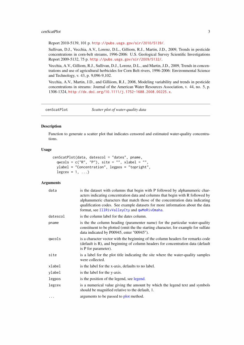
cenScatPlot Scatter plot of water-quality data

Description

Function to generate a scatter plot that indicates censored and estimated water-quality concentra-tions.

Usage

cenScatPlot(data, datescol = "dates", pname,qwcols = c("R", "P"), site = "", xlabel = "",ylabel = "Concentration", legpos = "topright",legcex = 1, ...)

Arguments

data is the dataset with columns that begin with P followed by alphanumeric char-acters indicating concentration data and columns that begin with R followed byalphanumeric characters that match those of the concentration data indicatingqualification codes. See example datasets for more information about the dataformat, see IllRivValleyCty and qwMoRivOmaha.

datescol is the column label for the dates column.

pname is the the column heading (paramenter name) for the particular water-qualityconstituent to be plotted (omit the the starting character, for example for sulfatedata indicated by P00945, enter "00945").

qwcols is a character vector with the beginning of the column headers for remarks code(default is R), and beginning of column headers for concentration data (defaultis P for parameter).

site is a label for the plot title indicating the site where the water-quality sampleswere collected.

xlabel is the label for the x-axis, defaults to no label.

ylabel is the label for the y-axis.

legpos is the position of the legend, see legend.

legcex is a numerical value giving the amount by which the legend text and symbolsshould be magnified relative to the default, 1.

... arguments to be passed to plot method.

http://pubs.usgs.gov/sir/2010/5139/


http://dx.doi.org/10.1111/j.1752-1688.2008.00225.x

4 combineData

Details

This function uses the qualification, or remark, column associated with water-quality concentrationvalues to indicate which samples are unqualified, which are estimated, and which are censored. Ablank remark field or an "_" indicates that the concentration value is not qualified; an "E" indicatesthe values has been estimated; and a less than symbol, "<", indicates the value has been censoredas less than a minimum reporting level. See Oblinger Childress (1999) for information on theminimum reporting level and the definition of "E" for U.S. Geological Survey data. Other usersmay have a different definition of the minimum reporting level, but censored values need to bequalified with a "<". Using the "E" code is optional.

Value

a scatter plot

Author(s)

Karen R. Ryberg

References

Oblinger Childress, C.J., Foreman, W.T., Connor, B.F., and Maloney, T.J., 1999, New reporting pro-cedures based on long-term method detection levels and some considerations for interpretations ofwater-quality data provided by the U.S. Geological Survey: U.S. Geological Survey Open-File Re-port 99–193, 19 p. (Also available at http://water.usgs.gov/owq/OFR_99-193/index.html.)

Examples

data(swData)# scatter plot of Simazine concentrationscenScatPlot(IllRivValleyCty, pname="04035")# scatter plot with many additional plotting argumentspar(las=1, tcl=0.5)cenScatPlot(IllRivValleyCty, pname="04035",

site="05586100 Illinois River at Valley City, IL",ylabel="Simazine concentration, in micrograms per liter",legcex=0.7, ylim=c(0,0.4), yaxs="i", cex.lab=0.9,cex.axis=0.9, xlim=c(as.Date("1996-01-01", "%Y-%m-%d"),as.Date("2012-01-01", "%Y-%m-%d")), xaxs="i", xaxt="n")

axdates<-c("1996-01-01", "2000-01-01", "2004-01-01", "2008-01-01","2012-01-01")

axis(1, as.Date(axdates, "%Y-%m-%d"),labels=c("1996", "2000", "2004", "2008", "2012"), cex.axis=0.9)

combineData Combine water-quality sample data and continuous ancillary vari-ables

Description

Function to combine water-quality sample data and continuous (daily) ancillary variables and dropunnecessary columns.

http://water.usgs.gov/owq/OFR_99-193/index.html

combineData 5

Usage

combineData(qwdat, cqwdat,qwcols = c("staid", "dates", "R", "P"))

Arguments

qwdat is the dataset containing water-quality sample data with columns that begin witha P (or other user-defined indicator) followed by alphanumeric characters. Thesecolumns are concentration data. In addition there need to be columns that beginwith an R (or other user- defined indicator) followed by alphanumeric charactersthat match those of the associated concentration data. The R columns containdata qualification codes. See example datasets for more information about thedata format, IllRivValleyCty and qwMoRivOmaha.

qwcols is a character vector with column headings for a station (location) identifier, adates column identifier, beginning of column headers for remarks code (defaultis R), and beginning of column headers for concentration data (default is P forparameter).

cqwdat is the dataset containing variables that can be used as explanatory variables forthe seawaveQ model. See example dataset for more information about the dataformat cqwMoRivOmaha. These are daily values with no missing values al-lowed between the first and the last date in the dataset.

Format

a dataframe with the number of rows equal to the number of rows in the dataframe indicated byqwdat. The number of columns depend on the two input data frames. Minimally there will be astation identification column, a dates column, a column of qualification codes, and a column ofwater-quality data.

Value

a dataframe

Note

The columns indicated by qwcols[1:2] are used to combined the datasets. The first column is thestation identifier and the second column is the date column. These two column headings must bethe same in the two datasets being combined and the dates in the datasets being combined must befor the class Date and be in the same format.

Author(s)

Karen R. Ryberg and Aldo V. Vecchia

Examples

data(swData)MoRivOmaha<-combineData(qwdat=qwMoRivOmaha, cqwdat=cqwMoRivOmaha,qwcols=c("staid", "dates", "R", "P"))

6 compwaveconv

compwaveconv Seasonal Wave Computation

Description

Function to compute seasonal wave.

Usage

compwaveconv(cmaxt, jmod, hlife, mclass = 1)

Arguments

cmaxt is the time of the maximum chemical concentration, decimal time in years.jmod is the choice of model or pulse input function, an integer 1 through 14.hlife is the model half-life in months, 1 to 4 monthsmclass has not been implemented yet, but will provide additional model options.

Value

a numeric vector of size 361 with discrete values of the seasonal wave for decimal season seq(0,1,1/360).

Note

The seasonal wave is a dimensionless, periodic function of time with an annual cycle, similar to amixture of sine and cosine functions often used to model seasonality in concentration data. How-ever, the seasonal wave is better suited for modeling seasonal behavior of pesticide data than amixture of sines and cosines. The pulse input function, represented by jmod, has either one or twodistinct application seasons (when pesticides may be transported to the stream) of lengths from 1 to6 months. Therefore, 56 (14x4) choices for the wave function are available. The numeric vector isa discrete approximation of the continuous wave function defined on the interval 0 to 1.

Author(s)

Aldo V. Vecchia

References

Vecchia, A.V., Martin, J.D. and Gilliom, R.J., 2008, Modeling variability and trends in pesticideconcentrations in streams: JAWRA Journal of the American Water Resources Association, v. 44,p. 1308–1324, http://onlinelibrary.wiley.com/doi/10.1111/j.1752-1688.2008.00225.x/abstract.

Examples

# evaluate seasonal wave for specified decimal seasons# these example decimal dates represent days at points 0.25, 0.5, and# 0.75 percent of the way through the year and the end of the yeardseas <- c(0.25, 0.5, 0.75, 1)swave <- compwaveconv(cmaxt=0.483, jmod=2, hlife=4, mclass=1)swave[floor(360 * dseas)]plot(seq(0,1,1/360),swave, typ="l")

http://onlinelibrary.wiley.com/doi/10.1111/j.1752-1688.2008.00225.x/abstract

http://onlinelibrary.wiley.com/doi/10.1111/j.1752-1688.2008.00225.x/abstract

cqwMoRivOmaha 7

cqwMoRivOmaha Continuously monitored (daily) data for 06610000 Missouri River atOmaha, Neb.

Description

Continuously monitored (daily) streamflow and sediment data for U.S. Geological Survey stream-gage 06610000 Missouri River at Omaha, Neb., and streamflow and sediment anomalies.

Usage

cqwMoRivOmaha

Format

A data frame containing 2,922 daily observations of two hydrologic variables, streamflow and sed-iment, and streamflow and sediment anomalies. There are eight variables.

staid character USGS Station identification numberdates date date water-quality sample collecteddflow numeric daily mean streamflow, cubic feet per secondflowa30 numeric 30-day streamflow anomalyflowa1 numeric 1-day streamflow anomalydsed numeric daily mean sediment concentration, milligrams per literseda30 numeric 30-day sediment anomalyseda1 numeric 1-day sediment anomaly

Details

The streamflow and sediment anomalies were generated using the R package waterData (Rybergand Vecchia, 2012).

Note

See Ryberg and Vecchia (2012) for more information on calculating the anomalies and for ad-ditional references documenting the use of streamflow anomalies in water-quality trend analysisstudies.

Source

Data provided by Patrick Phillips, U.S. Geological Survey, New York Water Science Center.

References

Ryberg, K.R. and Vecchia, A.V., 2012, waterData—An R package for retrieval, analysis, andanomaly calculation of daily hydrologic time series data, version 1.0.0: U.S. Geological SurveyOpen-File Report 2012–1168, 8 p. (Also available at http://pubs.usgs.gov/of/2012/1168/.)

Examples

data(swData)

http://pubs.usgs.gov/of/2012/1168/

8 examplecavdat

# summary of water-quality concentrationsapply(cqwMoRivOmaha[,3:8], 2, summary)

examplecavdat Example continuous ancillary variable data.

Description

This is an example of the continuous ancillary data that is passed internally to subfunctions offitswavecav. It is provided here for use with examples of internal functions.

Usage

examplecavdat

Format

A data frame containing 2,893 data variables and 30-day and 1-day streamflow anomalies (Rybergand Vecchia, 2012).

yrx numeric Yearmox numeric Monthdax numeric Dayjdayx numeric Julian day from first day water year for start year in fitswavecavflowa30 numeric 30-day streamflow anomalyflowa1 numeric 1-day streamflow anomaly

Source

Internal data captured from the following function call:

fitswavecav(cdat=modMoRivOmaha, cavdat=cqwMoRivOmaha,tanm="myexample", pnames=c("04041"), yrstart=1995,yrend=2003, tndbeg=1995, tndend=2003,iwcav=c("flowa30","flowa1"), dcol="dates",qwcols=c("R","P"))

References

Ryberg, K.R., and Vecchia, A.V., 2012, waterData–An R package for retrieval, analysis, and anomalycalculation of daily hydrologic time series data, version 1.0: U.S. Geological Survey Open-File Re-port 2012–1168, 8 p. (Also available at http://pubs.usgs.gov/of/2012/1168/.)

Examples

data(swData)head(examplecavdat)

http://pubs.usgs.gov/of/2012/1168/

examplecdatsub 9

examplecavmat Example continuous ancillary variable matrix.

Description

This is an example of the continuous ancillary matrix that is passed internally to subfunctions offitswavecav. It is provided here for use with examples of internal functions.

Usage

examplecavmat

Format

A matrix containing 115 30-day and 1-day streamflow anomalies (Ryberg and Vecchia, 2012).

flowa30 numeric 30-day streamflow anomalyflowa1 numeric 1-day streamflow anomaly

Source



Examples

data(swData)head(examplecavmat)

examplecdatsub Example water-quality data.

Description

This is an example of the water-quality data that is passed internally to subfunctions of fitswavecav.It is provided here for use with examples of internal functions.

Usage

examplecdatsub

10 examplecdatsub

Format

A data frame containing 115 observations of 10 variables. The date variables were internally calcu-lated. The columns R04041 and P04041 are a subset of qwMoRivOmaha and the 30-day and 1-daystreamflow and sediment anomalies are a subset of cqwMoRivOmaha.

examplecentmp 11

yrc numeric Yearmoc numeric Monthdac numeric Dayjdayc numeric Julian day from first day of start year in fitswavecavflowa30 numeric 30-day streamflow anomalyflowa1 numeric 1-day streamflow anomalyseda30 numeric 30-day sediment anomalyseda1 numeric 1-day sediment anomaly

Source



See Also

qwMoRivOmaha cqwMoRivOmaha

Examples

data(swData)head(examplecdatsub)

examplecentmp Example logical vector.

Description

This is an example of data that is passed internally to subfunctions of link{fitswavecav}. Thislogical vector indicates which water-quality values are censored. It is provided here for use withexamples of the internal functions.

Usage

examplecentmp

Format

A logical vector of 115 observations.

Source



12 exampleqwcols

Examples

data(swData)examplecentmp

exampleclog Example of logarithmically transformed concentration data.

Description

This is an example of data that is used internally by fitMod and passed to its subfunction seawaveQPlots.This numeric vector represents the base-10 logarithm of the water-quality concentrations. It is pro-vided here for use with examples of the internal functions.

Usage

exampleclog

Format

A numeric vector of 115 observations.

Source



Examples

data(swData)exampleclog

exampleqwcols Example data indicators.

Description

This is an example of the character vector used to indicate which columns represent qualificationcodes and which represent water-quality concentration data. It is provided here for use with exam-ples of the internal functions.

Usage

exampleqwcols

examplestpars 13

Format


Source



See Also

prepData fitMod

Examples

data(swData)exampleqwcols

examplestpars Example matrix for internal use.

Description

This is an example of data that is passed internally to subfunctions of fitswavecav. It is providedhere for use with examples of the internal functions.

Usage

examplestpars

Format

A numeric matrix of two rows and 14 columns.column description1 mclass, model class has not been implemented yet and is equal to 12 model chosen (a number 1-56), this number represents both the pulse input function and the half-life3 is the scale factor from the survreg.object 4 is the likelihood for the model chosen5 is the coefficient for the model intercept6 is the coefficient for the seasonal wave component of the model7 is the coefficient for the trend component of the model8 is the coefficient for the 30-day flow anomaly9 is the coefficient for the 1-day flow anomaly10 is the standard error for the intercept term11 is the standard error for the seasonal wave term12 is the standard error for the trend term13 is the standard error for the 30-day flow anomaly term

14 exampletndlin

14 is the standard error for the 1-day flow anomaly term15 is cmaxt, the decimal season of maximum concentration16 is the p-value for the trend line

Source



See Also

fitswavecav

Examples

data(swData)examplestpars

exampletndlin Example numeric vector used internally.

Description

This is an example of data that is passed internally to seawaveQPlots. This numeric vector containstrend coefficients for the water-quality samples. It is provided here for use with examples of theinternal functions.

Usage

exampletndlin

Format


Source



Examples

data(swData)head(exampletndlin)

exampletndlinpr 15

exampletndlinpr Example numeric vector used internally.

Description

This is an example of data that is passed internally to seawaveQPlots. This numeric vector con-tains trend coefficients for a continous water-quality prediction based on the continuous ancillaryvariables. It is provided here for use with examples of the internal functions.

Usage

exampletndlinpr

Format

A numeric vector of 2,893 observations.

Source



Examples

data(swData)head(exampletndlinpr)

exampletseas Example numeric vector used internally.

Description

This is an example of data that is passed internally to seawaveQPlots. This numeric vector con-tains decimal seasonal (0-1) values for the water-quality samples. It is provided here for use withexamples of the internal functions.

Usage

exampletseas

Format


16 exampletseaspr

Source



Examples

data(swData)head(exampletseas)

exampletseaspr Example numeric vector used internally.

Description

This is an example of data that is passed internally to seawaveQPlots. This numeric vector containsdecimal seasonal (0-1) values for the continuous ancillary data. It is provided here for use withexamples of the internal functions.

Usage

exampletseaspr

Format


Source



Examples

data(swData)head(exampletseaspr)

exampletyr 17

exampletyr Example numeric vector used internally.

Description

This is an example of data that is passed internally to seawaveQPlots. This numeric vector containsdecimal dates for the water-quality samples. It is provided here for use with examples of the internalfunctions.

Usage

exampletyr

Format


Source



Examples

data(swData)head(exampletyr)

exampletyrpr Example numeric vector used internally.

Description

This is an example of data that is passed internally to seawaveQPlots. This numeric vector containsdecimal dates for continuous ancillary variables. It is provided here for use with examples of theinternal functions.

Usage

exampletyrpr

Format


18 fitMod

Source



Examples

data(swData)head(exampletyrpr)

fitMod Internal function that fits the seawaveQ model.

Description

fitMod is called from within fitswavecav but can be invoked directly. It fits the seawaveQ modeland returns the results.

Usage

fitMod(cdatsub, cavdat, yrstart, yrend, tndbeg, tndend,tanm, pnames, qwcols, mclass = 1)

Arguments

cdatsub is the concentration data

cavdat is the continuous (daily) ancillary data

yrstart is the starting year of the analysis (treated as January 1 of that year).

yrend is the ending year of the analysis (treated as December 31 of that year).

tndbeg is the beginning (in whole or decimal years) of the trend period.

tndend is the end (in whole or decimal years) of the trend period.

tanm is a character identifier that names the trend analysis run. It is used to labeloutput files.

pnames is the parameter (water-quality constituents) to analyze (if using USGS parame-ters, omit the the starting ’P’, such as "00945" for sulfate).


mclass has not been implemented yet, but will provide additional model options.

fitswavecav 19

Value

a pdf file containing plots (see seawaveQPlots), a text file showing the best model survival regres-sion call and results, and a list. The first element of the list contains information about the data andthe model(s) selected (see examplestpars). The second element of the list contains the summary ofthe survival regression call. The third element of the list is itself a list containing the observed con-centrations (censored and uncensored) and the predicted concentrations used by seawaveQPlots togenerate the plots.

Author(s)

Aldo V. Vecchia and Karen R. Ryberg

Examples

data(swData)myRes <- fitMod(cdatsub=examplecdatsub, cavdat=examplecavdat,yrstart=1995, yrend=2003, tndbeg=1995, tndend=2003, tanm="myfit3",pnames=c("04041"), qwcols=c("R", "P"))

fitswavecav Fit seasonal wave and continuous ancillary data for trend analysis

Description

Function to prepare data and fit the seawaveQ model.

Usage

fitswavecav(cdat, cavdat, tanm = "trend1", pnames,yrstart = 0, yrend = 0, tndbeg = 0, tndend = 0,iwcav = c("none"), dcol = "dates",qwcols = c("R", "P"), mclass = 1)

Arguments

cdat is the concentration data


tanm is a character identifier that names the trend analysis run. It is used to labeloutput files.

pnames are the parameters (water-quality constituents) to analyze (omit the the startingcharacter, for example for sulfate data indicated by P00945, enter "00945").

yrstart is the starting year of the analysis (treated as January 1 of that year). Zeromeans the start date will be determined by the start date of cavdat, the continuousancillary data.

yrend is the ending year of the analysis (treated as December 31 of that year). Zeromeans the end date will be determined by the end date of cavdat, the continuousancillary data.

tndbeg is the beginning (in whole or decimal years) of the trend period. Zero means thebegin date will be the beginning of the concentration data, cdat.

20 fitswavecav

tndend is the end of the trend (treated as December 31 of that year). Zero means theend date will be the end of the concentration data, cdat.

iwcav is a character vector indicating which continuous ancillary variables to include,if none are used for analysis, use iwcav=c("none").

dcol is the column name for the dates, should be the same for both cdat and cavdat


mclass has not been implemented yet but will provide additional model options.

Format

The data frame returned has one row for each parameter analyzed and the number of columns de-pend on the number of continuous ancillary variables used. The general format is as follows:

pname character Parameter analyzedmclass numeric Currently a value of 1jmod numeric The choice of pulse input function, an integer 1–14.hlife numeric the model half-life in months, an integer, 1 to 4 monthscmaxt numeric the decimal season of maximum concentrationscl numeric the scale factor from the survreg.objectloglik numeric the log-likelihood for the modelcint numeric coefficient for model interceptcwave numeric coefficient for the seasonal wavectnd numeric coefficient for the trend component of modelc[alphanumeric] numeric 0 or more coefficients for the continuous ancillary variablesseint numeric standard error for the interceptsewave numeric standard error for the seasonal wavesetnd numeric standard error for the trendse[alphanumeric] numeric 0 or more standard errors for the continuous ancillary variablespvaltnd numeric the p-value for the trend line

Details

Fits the seawaveQ model (Vecchia and others, 2008) using a seasonal wave and continuous ancillaryvariables (streamflow anomalies and other continuous variables such as conductivity or sediment)to model water quality.

Value

a pdf file containing plots of the data and modeled concentration, a text file containing a summaryof the survival regression call for each model selected, and a list. The first element of the list is adata frame described under format. The second element of the list is the summary of the survivalregression call. The third element is the observed concentration data (censored and uncensored).The fourth element is the concentration data predicted by the model. The fifth element providessummary statistics for the predicted concentrations.

fitswavecav 21

Note

The assumed data format is one with columns for water-quality concentration values and a relatedcolumn for qualification of those values, such as in the case of left-censored values less than aparticular value. For example, a water-quality sample was collected and the laboratory analysisindicated that the concentration was less than 0.01 micrograms per liter. The USGS parametercode for simazine is 04035 (U.S. Geological Survey, 2013b). When the data are retrieved throughthe National Water Information System: Web Interface (http://waterdata.usgs.gov/nwis; U.S.Geological Survey, 2013a), the concentration values are in a column labeled P04035 and the qual-ification information, or remark codes, are in a column labeled R04035. To use this function, theargument pnames would be the unique identifier for simazine values and qualifications, 04035, andthe qwcols argument would be c("R", "P") to indicate that the qualification column starts with an Rand the values column starts with a P.Other users may have data in different format that can be changed to use with this function. Forexample, a user may have concentration values and qualification codes in one column, such as acolumn labeled simzaine with the values 0.05, 0.10, <0.01, <0.01, and 0.90. In this case, the lessthans and any other qualification codes should be placed in a separate column. The column namesfor the qualification codes and the concentration values should be the same with the exception ofdifferent beginning letters to indicate which column is which. The columns could be named Rsi-mazine and Psimazine. Then the argument pnames = "simazine" and the argument qwcols = c("R","P").Users should exercise caution when their water-quality data have multiple censoring limits and maywant to recensor the data to a single censoring level. Censoring and recensoring issues are discussedin the text and Appendix 1 of Ryberg and others (2010).

Author(s)


References

Ryberg, K.R., Vecchia, A.V., Martin, J.D., and Gilliom, R.J., 2010, Trends in pesticide concentra-tions in urban streams in the United States, 1992–2008: U.S. Geological Survey Scientific Investi-gations Report 2010-5139, 101 p. (Also available at http://pubs.usgs.gov/sir/2010/5139/.)

U.S. Geological Survey, 2013a, National Water Information System: Web Interface, accessedFebaruary 26, 2013, at http://waterdata.usgs.gov.

U.S. Geological Survey, 2013b, Parameter code definition: National Water Information System:Web Interface, accessed Febaruary 26, 2013, at http://nwis.waterdata.usgs.gov/usa/nwis/pmcodes.

Vecchia, A.V., Martin, J.D., and Gilliiom, R.J., 2008, Modeling variability and trends in pesticideconcentrations in streams: Journal of the American Water Resources Association, v. 44, no. 5, p.1308-1324, http://dx.doi.org/10.1111/j.1752-1688.2008.00225.x.

See Also

The functions that fitswavecav calls internally:prepData and fitMod.

Examples

data(swData)modMoRivOmaha<-combineData(qwdat=qwMoRivOmaha, cqwdat=cqwMoRivOmaha)myfit1 <- fitswavecav(cdat=modMoRivOmaha, cavdat=cqwMoRivOmaha,

http://waterdata.usgs.gov/nwis


http://waterdata.usgs.gov

http://nwis.waterdata.usgs.gov/usa/nwis/pmcodes

http://nwis.waterdata.usgs.gov/usa/nwis/pmcodes

http://dx.doi.org/10.1111/j.1752-1688.2008.00225.x

22 IllRivValleyCty

tanm="myfit1", pnames=c("04035", "04037", "04041"), yrstart=1995,yrend=2003, tndbeg=1995, tndend=2003, iwcav=c("flowa30","flowa1"),dcol="dates", qwcols=c("R","P"))myfit2 <- fitswavecav(cdat=modMoRivOmaha, cavdat=cqwMoRivOmaha,tanm="myfit2", pnames=c("04035", "04037", "04041"), yrstart=1995,yrend=2003, tndbeg=1995, tndend=2003, iwcav=c("seda30","seda1"),dcol="dates", qwcols=c("R","P"))## Not run:

myfit3 <- fitswavecav(cdat=modMoRivOmaha, cavdat=cqwMoRivOmaha,tanm="myfit3", pnames=c("04035", "04037", "04041"), yrstart=1995,yrend=2003, tndbeg=1995, tndend=2003, iwcav=c("flowa30","flowa1","seda30", "seda1"), dcol="dates", qwcols=c("R","P"))

## End(Not run)# trend model resultsmyfit1[[1]]# example regression callmyfit1[[2]][[1]]# first few lines of observed concentrationshead(myfit1[[3]])# first few lines of predicted concentrationshead(myfit1[[4]])# summary statistics for predicted concentrationshead(myfit1[[5]])

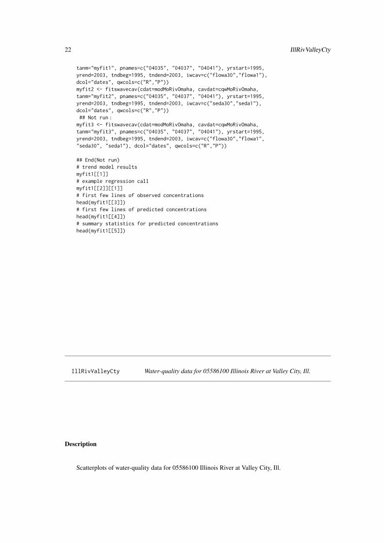
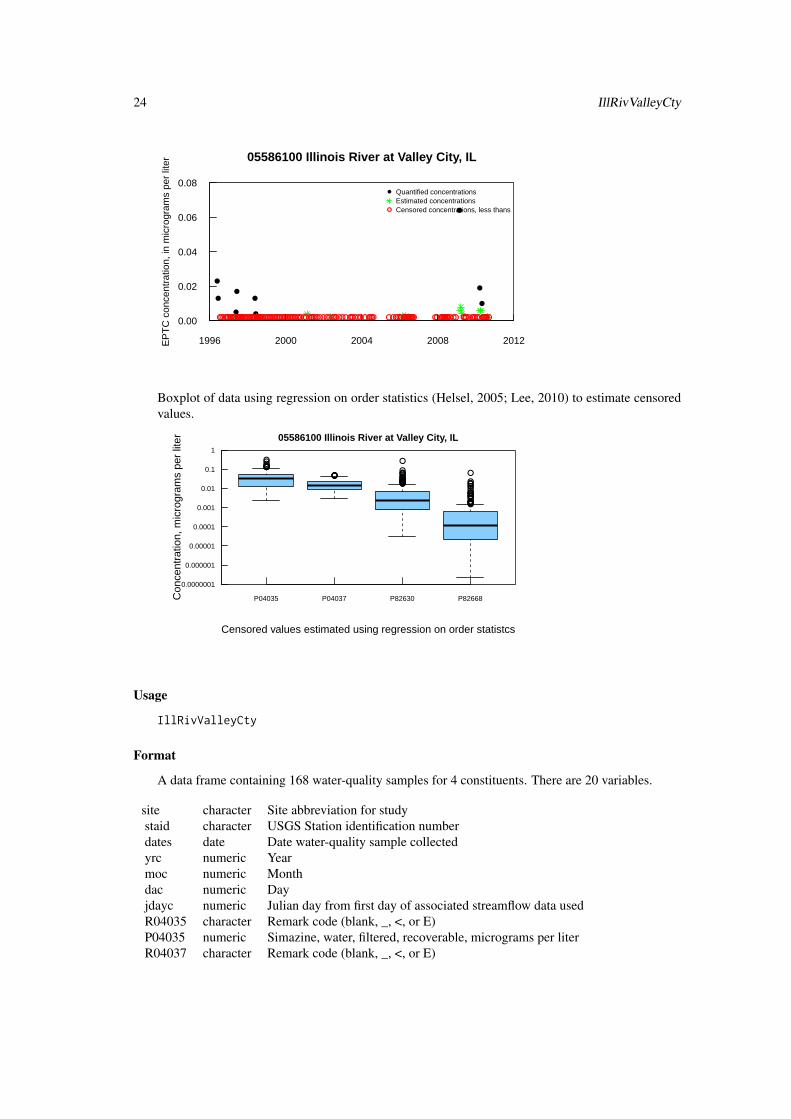
IllRivValleyCty Water-quality data for 05586100 Illinois River at Valley City, Ill.

Description

Scatterplots of water-quality data for 05586100 Illinois River at Valley City, Ill.

IllRivValleyCty 23

0.0

0.1

0.2

0.3

0.4

Sim

azin

e co

ncen

trat

ion,

in m

icro

gram

s pe

r lit

er

●

●●

●●●●

●

●●●●●●

●●

●●●●●●●●●

●

●●●●

●●

●

●

●●●●●●●●

●

●

●

●●●

●●●●●●

●●●●●

●

●

●●●

●

●

●

●

●●●

●

●

●●●●

●

●

●

●

●

●

●●●●

●●

●

●●●

●●●

●

●●●

●

●●●●

●

●●●●● ●●

●

●

●●●●

●●

●●

●

●

●

●

●

●●●●

●●●

●

●●●●

●●●●●●●

●●●●●●●● ●● ●● ● ●

●

●

Quantified concentrationsEstimated concentrationsCensored concentrations, less thans

05586100 Illinois River at Valley City, IL

1996 2000 2004 2008 2012

0.00

0.01

0.02

0.03

0.04

0.05

0.06

Pro

met

on c

once

ntra

tion,

in m

icro

gram

s pe

r lit

er

●

●

●●

●

●●●

●

●

●

●●

●

●

●

●

●●

● ●●

●●

●●●

●

●

●

●●

●●●

●

● ●

●●●●

●

●

●

●

●

●

●

●

●

●

●

●

●●

●●

●

● ●●

●

●

●●

●●●●

●

●

●

●

●

●●

●

●● ●●●●

●

●

●●

●●●

●

●●

●

●

●● ● ● ●

●

●



1996 2000 2004 2008 2012

0.00

0.05

0.10

0.15

0.20

0.25

0.30

Met

ribuz

in c

once

ntra

tion,

in m

icro

gram

s pe

r lit

er

●

●

●●

●

●●

●

●

●

● ●● ●

● ●● ● ●● ●

●

●●●

●●●

●●●●●●●●●●●●●●●●●●●●●●●●●●●●●●●●●●●●●●●●●●●●●●●●●●● ●●●●●●●●●●●●●●●●●●●●●●●●●●●●●●●●●●●●●●●●●●●●●●●●●● ●●●●●●●●●●●●●●●●●●●●●●●●●●●●●●●●

●

●



1996 2000 2004 2008 2012

24 IllRivValleyCty

0.00

0.02

0.04

0.06

0.08

EP

TC

con

cent

ratio

n, in

mic

rogr

ams

per

liter

●

●

●

●●

●

●

●

●

●●●●●●●●●●●●●●●●●●●●●●●●●●●●●●●●●●●●●●●●●●●●●●●●●●●●●●●●●●●●●●●●●●●●●●●●●●●●●●●●●●●●●●●●●●●● ●●●●●●●●●●●●●●●●●● ●●●●●●●●●●●●●● ●●●●●●●●●●●●●●●●●

●

●



1996 2000 2004 2008 2012

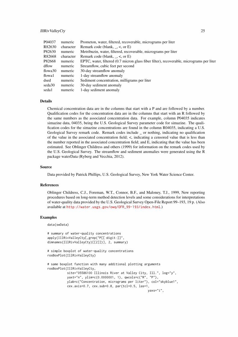
Boxplot of data using regression on order statistics (Helsel, 2005; Lee, 2010) to estimate censoredvalues.

●●●●●●●●●

●●●●

●●●●●●●●●●●●●●●●●●●●●●

●

●●●●●●●●●●●●●●●●●●●●●●●●

●

P04035 P04037 P82630 P82668Con

cent

ratio

n, m

icro

gram

s pe

r lit

er

Censored values estimated using regression on order statistcs


0.0000001

0.000001

0.00001

0.0001

0.001

0.01

0.1

1

Usage

IllRivValleyCty

Format

A data frame containing 168 water-quality samples for 4 constituents. There are 20 variables.

site character Site abbreviation for studystaid character USGS Station identification numberdates date Date water-quality sample collectedyrc numeric Yearmoc numeric Monthdac numeric Dayjdayc numeric Julian day from first day of associated streamflow data usedR04035 character Remark code (blank, _, <, or E)P04035 numeric Simazine, water, filtered, recoverable, micrograms per literR04037 character Remark code (blank, _, <, or E)

IllRivValleyCty 25

P04037 numeric Prometon, water, filtered, recoverable, micrograms per literR82630 character Remark code (blank, _, <, or E)P82630 numeric Metribuzin, water, filtered, recoverable, micrograms per literR82668 character Remark code (blank, _, <, or E)P82668 numeric EPTC, water, filtered (0.7 micron glass fiber filter), recoverable, micrograms per literdflow numeric Streamflow, cubic feet per secondflowa30 numeric 30-day streamflow anomalyflowa1 numeric 1-day streamflow anomalydsed numeric Sediment concentration, milligrams per literseda30 numeric 30-day sediment anomalyseda1 numeric 1-day sediment anomaly

Details

Chemical concentration data are in the columns that start with a P and are followed by a number.Qualification codes for the concentration data are in the columns that start with an R followed bythe same numbers as the associated concentration data. For example, column P04035 indicatessimazine data, 04035, being the U.S. Geological Survey parameter code for simazine. The quali-fication codes for the simazine concentrations are found in the column R04035, indicating a U.S.Geological Survey remark code. Remark codes include _ or nothing, indicating no qualificationof the value in the associated concentration field; <, indicating a censored value that is less thanthe number reported in the associated concentration field; and E, indicating that the value has beenestimated. See Oblinger Childress and others (1999) for information on the remark codes used bythe U.S. Geological Survey. The streamflow and sediment anomalies were generated using the Rpackage waterData (Ryberg and Vecchia, 2012).

Source


References

Oblinger Childress, C.J., Foreman, W.T., Connor, B.F., and Maloney, T.J., 1999, New reportingprocedures based on long-term method detection levels and some considerations for interpretationsof water-quality data provided by the U.S. Geological Survey Open-File Report 99–193, 19 p. (Alsoavailable at http://water.usgs.gov/owq/OFR_99-193/index.html.)

Examples

data(swData)

# summary of water-quality concentrationsapply(IllRivValleyCty[,grep("P[[:digit:]]",dimnames(IllRivValleyCty)[[2]])], 2, summary)

# simple boxplot of water-quality concentrationsrosBoxPlot(IllRivValleyCty)

# same boxplot function with many additional plotting argumentsrosBoxPlot(IllRivValleyCty,

site="05586100 Illinois River at Valley City, Ill.", log="y",yaxt="n", ylim=c(0.0000001, 1), qwcols=c("R", "P"),ylab=c("Concentration, micrograms per liter"), col="skyblue1",cex.axis=0.7, cex.sub=0.8, par(tcl=0.5, las=1,

yaxs="i",


26 IllRivValleyCty

mgp=c(3,0.5,0),mar=c(5,5,2,2),cex.main=0.9))

axis(2, at=c(0.0000001, 0.000001, 0.00001, 0.0001, 0.001, 0.01, 0.1, 1),labels=c("0.0000001", "0.000001", "0.00001", "0.0001", "0.001", "0.01",

"0.1", "1"), cex.axis=0.7)

# scatter plot of simazine concentrationscenScatPlot(IllRivValleyCty, pname="04035")

# scatter plot with many additional plotting argumentspar(las=1, tcl=0.5)cenScatPlot(IllRivValleyCty, pname="04035",

site="05586100 Illinois River at Valley City, Ill.",ylabel="Simazine concentration, in micrograms per liter",legcex=0.7,ylim=c(0,0.4), yaxs="i", cex.lab=0.9, cex.axis=0.9,xlim=c(as.Date("1996-01-01"), as.Date("2012-01-01")),xaxs="i", xaxt="n")

axdates<-c("1996-01-01", "2000-01-01", "2004-01-01", "2008-01-01","2012-01-01")

axis(1, as.Date(axdates), labels=c("1996", "2000", "2004", "2008","2012"), cex.axis=0.9)

# Prometon scatter plotcenScatPlot(IllRivValleyCty, pname="04037",

site="05586100 Illinois River at Valley City, Ill.",ylabel="Prometon concentration, in micrograms per liter",legcex=0.7,ylim=c(0,0.06), yaxs="i", cex.lab=0.9, cex.axis=0.9,xlim=c(as.Date("1996-01-01"),

as.Date("2012-01-01")), xaxs="i",xaxt="n")

axdates<-c("1996-01-01", "2000-01-01", "2004-01-01", "2008-01-01","2012-01-01")


# Metribuzin scatter plotcenScatPlot(IllRivValleyCty, pname="82630",

site="05586100 Illinois River at Valley City, Ill.",ylabel="Metribuzin concentration, in micrograms per liter",legcex=0.7,ylim=c(0,0.3), yaxs="i", cex.lab=0.9, cex.axis=0.9,xlim=c(as.Date("1996-01-01"),


axdates<-c("1996-01-01", "2000-01-01", "2004-01-01", "2008-01-01","2012-01-01")


# EPTC scatter plotcenScatPlot(IllRivValleyCty, pname="82668",

site="05586100 Illinois River at Valley City, Ill.",ylabel="EPTC concentration, in micrograms per liter",legcex=0.7, ylim=c(0,0.08), yaxs="i", cex.lab=0.9,cex.axis=0.9, xlim=c(as.Date("1996-01-01"),

prepData 27

as.Date("2012-01-01")), xaxs="i", xaxt="n")axdates<-c("1996-01-01", "2000-01-01", "2004-01-01", "2008-01-01",

"2012-01-01")axis(1, as.Date(axdates), labels=c("1996", "2000", "2004", "2008","2012"),

cex.axis=0.9)

prepData Prepares concentration data and continuous ancillary data

Description

prepData is usually called from within fitswavecav but can be invoked directly. It performs somedate calculations, removes rows with missing values for concentration or continous variables, andreturns the the concentration and continuous ancillary data to be used by fitswavecav and its otherinternal functions.

Usage

prepData(cdat, cavdat, yrstart, yrend, dcol, pnames,iwcav, qwcols)

Arguments

cdat is the concentration data.

cavdat is the continuous (daily) ancillary data.

yrstart is the starting year of the analysis (treated as January 1 of that year). Zeromeans the start date will be determined by the start date of cavdat, the continuousancillary data.

yrend is the ending year of the analysis (treated as December 31 of that year). Zeromeans the end date will be determined by the end date of cavdat, the continuousancillary data.

dcol is the column name for the dates, should be the same for both cdat and cavdat.

pnames are the parameters (water-quality constituents) to analyze (if using USGS pa-rameters, omit the the starting ’P’, such as "00945" for sulfate).

iwcav is a character variable indicating which continuous ancillary variables to include,if none use iwcav=c("none").


Value

a list. The first element is the concentration data with additional date information, missing valuesremoved, and extra columns removed. The second element is the continuous ancillary data withadditional date information, missing values removed, and extra columns removed.

Author(s)


28 qwMoRivOmaha

Examples

data(swData)modMoRivOmaha<-combineData(qwdat=qwMoRivOmaha, cqwdat=cqwMoRivOmaha)preppedDat <- prepData(modMoRivOmaha, cqwMoRivOmaha, yrstart=1995,yrend=2003, dcol="dates", pnames=c("04035", "04037", "04041"),iwcav=c("flowa30","flowa1"), qwcols=c("R","P"))

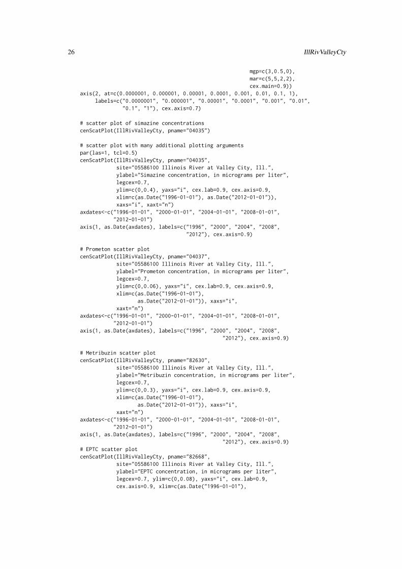
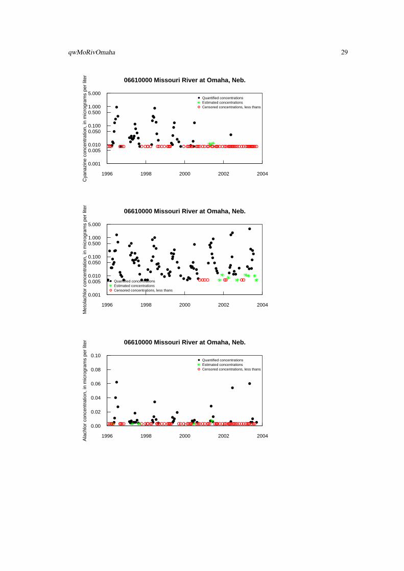
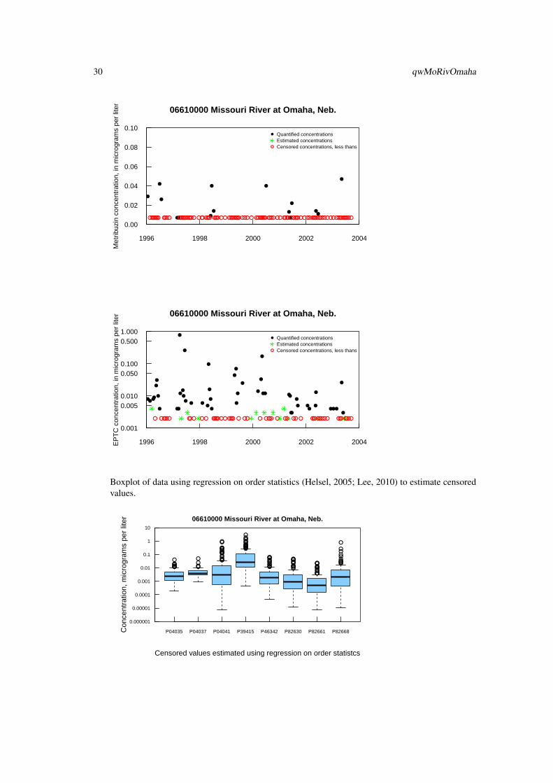
qwMoRivOmaha Water-quality data for 06610000 Missouri River at Omaha, Nebr.

Description

Scatterplots of water-quality data for 06610000 Missouri River at Omaha, Nebr.

0.00

0.02

0.04

0.06

0.08

0.10

Sim

azin

e co

ncen

trat

ion,

in m

icro

gram

s pe

r lit

er

●●

●

●●●

●●●●● ●

●

●● ●●●

● ●● ●

●

●

●

●

●●●●●●● ●●●● ●●● ●●●●● ●●●●●●●● ●●●● ●●●●●●●●●●●●●●●●●●●●●●●●●●●●●●●●●●●●● ●●●●●●●●

●

●


06610000 Missouri River at Omaha, Neb.

1996 1998 2000 2002 2004

0.00

0.02

0.04

0.06

0.08

0.10

Pro

met

on c

once

ntra

tion,

in m

icro

gram

s pe

r lit

er

●

●

● ●● ●●● ●●●● ●●●●●●●●●● ● ● ● ●●● ● ●●●● ●●● ●●

●

●



1996 1998 2000 2002 2004

qwMoRivOmaha 29

0.001

0.0050.010

0.0500.100

0.5001.000

5.000

Cya

nazi

ne c

once

ntra

tion,

in m

icro

gram

s pe

r lit

er

●●●

●

●●

●

●

●

●

●

●●●●

●

●

●

●

●

●●

●

●

●●

●

●

●

●●●

●

●

●

●●

● ●

●

●

●

●

●●● ●●● ● ●●●● ●●●●●●●● ● ●●●●● ●●●●●●●● ●● ●●●●●●●●●●●●●●●●●●●●●●●●●●●●●●●●

●

●



1996 1998 2000 2002 2004

0.001

0.0050.010

0.0500.100

0.5001.000

5.000

Met

olac

hlor

con

cent

ratio

n, in

mic

rogr

ams

per

liter

●

●

●●

●

●●

●●

●

●

●●●●

●

●

●

●

●●●

●

●●●

●

●

● ●●

●●

●

●

●

●

●

●

●

●

●●

●●

●●●●

●

●●●

●

●

●

●● ●

●●

●●●

●

●

●

●●

●

●

●●

●

●●

●

●

●●● ●

●●

●

●

●

●●●

● ●●

●

●

●

●

●●

●●●● ●● ●●●

●



1996 1998 2000 2002 2004

0.00

0.02

0.04

0.06

0.08

0.10

Ala

chlo

r co

ncen

trat

ion,

in m

icro

gram

s pe

r lit

er

●

●

●

●

●

●●●●●●

●

●●●

●●

●

●

●●

●

●●●

●

●●●

● ●

●

●

●

●

●

●

●●●

●●●●●● ●●●● ● ●●●●● ●●●●●●●●●● ●●● ●●●●● ●●●●●●●● ●●●●●●●●●●●●●●●●●●●●●●●●●●●

●

●



1996 1998 2000 2002 2004

30 qwMoRivOmaha

0.00

0.02

0.04

0.06

0.08

0.10

Met

ribuz

in c

once

ntra

tion,

in m

icro

gram

s pe

r lit

er

●

●

●

●● ●

●

●

●

●

●

●

●●

●

●●●●●●●● ●●●● ●●●●●●●●●●●● ●●●●●●● ●●●●●●●●●●●●●●●●●●● ●●●●●●●●●●●●●●●●●●●●●●●●●●●●●●●●●●●●●●●●●●●●●●●●●●

●

●



1996 1998 2000 2002 2004

0.001

0.0050.010

0.0500.100

0.5001.000

EP

TC

con

cent

ratio

n, in

mic

rogr

ams

per

liter

●●●●

●●

●

● ●●

●

●●

●

●

● ● ●●

●

●

●

●

●

●

●

●

●

●

●

●

●● ●●

●●

●

● ●●

●

●

●●●

●

●

● ●●●●● ●●● ●● ●●●●●●●●●●● ● ●● ● ●●●● ● ●● ●● ● ●●●●●●●●● ●●● ●●●●

●

●



1996 1998 2000 2002 2004

Boxplot of data using regression on order statistics (Helsel, 2005; Lee, 2010) to estimate censoredvalues.

●●●●●●●●

●●●● ●●●

●●●●●●●●●●●●

●●

●●●●●●●●●●●●●●●●

●●●●●●●●●●●●

●●●●●●●●●●●●

●●●●●●●●●●●●●●●● ●●●

●●●●●●●

●

P04035 P04037 P04041 P39415 P46342 P82630 P82661 P82668Con

cent

ratio

n, m

icro

gram

s pe

r lit

er

Censored values estimated using regression on order statistcs


0.000001

0.00001

0.0001

0.001

0.01

0.1

1

10

qwMoRivOmaha 31

Usage

qwMoRivOmaha

Format

A data frame containing 115 water-quality samples for eight chemical constituents. There are 20variables.

staid character USGS Station identification numberdates date Date water-quality sample collectedtimes numeric Time sample was collectedR04035 character Remark code (blank, _, <, or E)P04035 numeric Simazine, water, filtered, recoverable, micrograms per literR04037 character Remark code (blank, _, <, or E)P04037 numeric Prometon, water, filtered, recoverable, micrograms per literR04041 character Remark code (blank, _, <, or E)P04041 numeric Cyanazine, water, filtered, recoverable, micrograms per literR39415 character Remark code (blank, _, <, or E)P39415 numeric Metolachlor, water, filtered, recoverable, micrograms per literR46342 character Remark code (blank, _, <, or E)P46342 numeric Alachlor, water, filtered, recoverable, micrograms per literR82630 character Remark code (blank, _, <, or E)P82630 numeric Metribuzin, water, filtered, recoverable, micrograms per literR82661 character Remark code (blank, _, <, or E)P82661 numeric Trifluralin, water, filtered (0.7 micron glass fiber filter), recoverable, micrograms per literR82668 character Remark code (blank, _, <, or E)P82668 numeric EPTC, water, filtered (0.7 micron glass fiber filter), recoverable, micrograms per liter

Details

Chemical concentration data are in the columns that start with a P and are followed by a number.Qualification codes for the concentration data are in the columns that start with an R followed bythe same numbers as the associated concentration data. For example, column P04035 indicatessimazine data, 04035, being the U.S. Geological Survey parameter code for simazine. The quali-fication codes for the simazine concentrations are found in the column R04035, indicating a U.S.Geological Survey remark code. Remark codes include _ or nothing, indicating no qualificationof the value in the associated concentration field; <, indicating a censored value that is less thanthe number reported in the associated concentration field; and E, indicating that the value has beenestimated. See Oblinger Childress and others (1999) for information on the remark codes used bythe U.S. Geological Survey.

Source


References

Oblinger Childress, C.J., Foreman, W.T., Connor, B.F., and Maloney, T.J., 1999, New reportingprocedures based on long-term method detection levels and some considerations for interpretationsof water-quality data provided by the U.S. Geological Survey Open-File Report 99–193, 19 p. (Alsoavailable at http://water.usgs.gov/owq/OFR_99-193/index.html.)


32 qwMoRivOmaha

Examples

data(swData)

# summary of water-quality concentrationsapply(qwMoRivOmaha[,grep("P[[:digit:]]",dimnames(qwMoRivOmaha)[[2]])],2, summary)

# simple boxplot of water-quality concentrationsrosBoxPlot(qwMoRivOmaha, qwcols=c("R", "P"))

# same boxplot function with many additional plotting argumentsrosBoxPlot(qwMoRivOmaha, site="06610000 Missouri River at Omaha, Nebr.",

log="y", yaxt="n", ylim=c(0.000001, 10), qwcols=c("R", "P"),ylab=c("Concentration, micrograms per liter"), col="skyblue1",cex.axis=0.7, cex.sub=0.8, par(tcl=0.5, las=1,

yaxs="i",mgp=c(3,0.5,0),mar=c(5,5,2,2),cex.main=0.9))

axis(2, at=c(0.000001, 0.00001, 0.0001, 0.001, 0.01, 0.1, 1, 10),labels=c("0.000001", "0.00001", "0.0001", "0.001", "0.01",

"0.1", "1", "10"), cex.axis=0.7)

# scatter plot of Simazine concentrationscenScatPlot(qwMoRivOmaha, pname="04035")

# scatter plot with many additional plotting argumentspar(las=1, tcl=0.5)cenScatPlot(qwMoRivOmaha, pname="04035",

site="06610000 Missouri River at Omaha, Nebr.",ylabel="Simazine concentration, in micrograms per liter",legcex=0.7, qwcols=c("R", "P"),ylim=c(0,0.1), yaxs="i", cex.lab=0.9, cex.axis=0.9,xlim=c(as.Date("1996-01-01"), as.Date("2004-01-01")),xaxs="i", xaxt="n")

axdates<-c("1996-01-01", "1998-01-01", "2000-01-01", "2002-01-01","2004-01-01")


# Prometon scatter plotcenScatPlot(qwMoRivOmaha, pname="04037",

site="06610000 Missouri River at Omaha, Nebr.",ylabel="Prometon concentration, in micrograms per liter",legcex=0.7, qwcols=c("R", "P"),ylim=c(0,0.1), yaxs="i", cex.lab=0.9, cex.axis=0.9,xlim=c(as.Date("1996-01-01"),


axdates<-c("1996-01-01", "1998-01-01", "2000-01-01", "2002-01-01","2004-01-01")


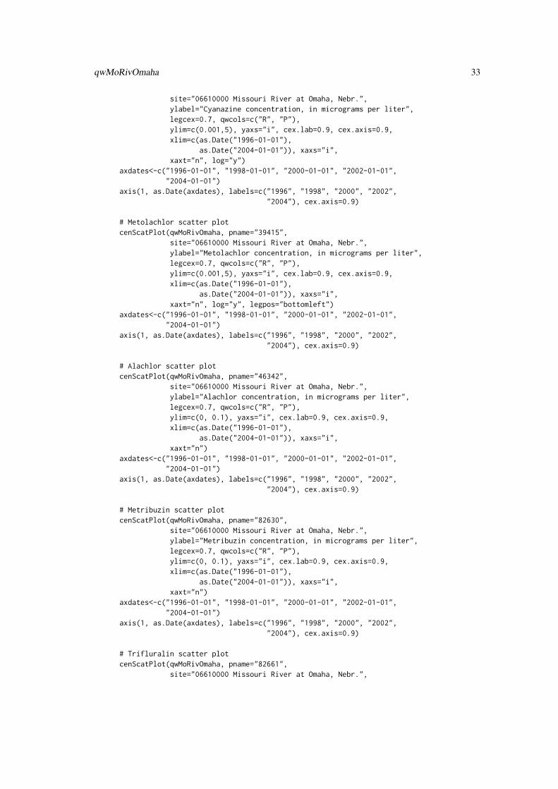
# Cyanazine scatter plotcenScatPlot(qwMoRivOmaha, pname="04041",

qwMoRivOmaha 33

site="06610000 Missouri River at Omaha, Nebr.",ylabel="Cyanazine concentration, in micrograms per liter",legcex=0.7, qwcols=c("R", "P"),ylim=c(0.001,5), yaxs="i", cex.lab=0.9, cex.axis=0.9,xlim=c(as.Date("1996-01-01"),

as.Date("2004-01-01")), xaxs="i",xaxt="n", log="y")

axdates<-c("1996-01-01", "1998-01-01", "2000-01-01", "2002-01-01","2004-01-01")


# Metolachlor scatter plotcenScatPlot(qwMoRivOmaha, pname="39415",

site="06610000 Missouri River at Omaha, Nebr.",ylabel="Metolachlor concentration, in micrograms per liter",legcex=0.7, qwcols=c("R", "P"),ylim=c(0.001,5), yaxs="i", cex.lab=0.9, cex.axis=0.9,xlim=c(as.Date("1996-01-01"),

as.Date("2004-01-01")), xaxs="i",xaxt="n", log="y", legpos="bottomleft")

axdates<-c("1996-01-01", "1998-01-01", "2000-01-01", "2002-01-01","2004-01-01")


# Alachlor scatter plotcenScatPlot(qwMoRivOmaha, pname="46342",

site="06610000 Missouri River at Omaha, Nebr.",ylabel="Alachlor concentration, in micrograms per liter",legcex=0.7, qwcols=c("R", "P"),ylim=c(0, 0.1), yaxs="i", cex.lab=0.9, cex.axis=0.9,xlim=c(as.Date("1996-01-01"),


axdates<-c("1996-01-01", "1998-01-01", "2000-01-01", "2002-01-01","2004-01-01")


# Metribuzin scatter plotcenScatPlot(qwMoRivOmaha, pname="82630",

site="06610000 Missouri River at Omaha, Nebr.",ylabel="Metribuzin concentration, in micrograms per liter",legcex=0.7, qwcols=c("R", "P"),ylim=c(0, 0.1), yaxs="i", cex.lab=0.9, cex.axis=0.9,xlim=c(as.Date("1996-01-01"),


axdates<-c("1996-01-01", "1998-01-01", "2000-01-01", "2002-01-01","2004-01-01")


# Trifluralin scatter plotcenScatPlot(qwMoRivOmaha, pname="82661",

site="06610000 Missouri River at Omaha, Nebr.",

34 rosBoxPlot

ylabel="Trifluralin concentration, in micrograms per liter",legcex=0.7, qwcols=c("R", "P"),ylim=c(0,0.03), yaxs="i", cex.lab=0.9, cex.axis=0.9,xlim=c(as.Date("1996-01-01"),


axdates<-c("1996-01-01", "1998-01-01", "2000-01-01", "2002-01-01","2004-01-01")


# EPTC scatter plotcenScatPlot(qwMoRivOmaha, pname="82668",

site="06610000 Missouri River at Omaha, Nebr.",ylabel="EPTC concentration, in micrograms per liter",legcex=0.7, qwcols=c("R", "P"),ylim=c(0.001,1), yaxs="i", cex.lab=0.9, cex.axis=0.9,xlim=c(as.Date("1996-01-01"),

as.Date("2004-01-01")), xaxs="i",xaxt="n", log="y")

axdates<-c("1996-01-01", "1998-01-01", "2000-01-01", "2002-01-01","2004-01-01")


rosBoxPlot Boxplot of water-quality data

Description

Function to create boxplots of water-quality data that include censored values.

Usage

rosBoxPlot(data, site = "", qwcols = c("R", "P"), ...)

Arguments

data is the dataset with columns that begin with P followed by a number indicat-ing concentration data and columns that begin with R followed by numbers thatmatch those of the concentration data indicating qualification codes. See exam-ple data sets for more information about the data format, IllRivValleyCty andqwMoRivOmaha.


site is a label for the plot title indicating the site where the water-quality sampleswere collected.

... arguments to be passed to plot method.

rosBoxPlot 35

Details

This function determines the columns within the data set that have concentration data, based onthem having column headings that start with P (or a user-specificed indicater in the second elementof the qwcols argument) followed by a number. The function determines the associated remark, orqualification columns, based on them having column headings that start with R (or a user-specificedindicater in the first element of the qwcols argument) followed by numbers that match the associatedconcentration data. Then it determines which values are censored, indicated by a less than symbol inthe R columns, performs regression on order statistics, ros, using the NADA package, and estimatesvalues for the censored concentrations for constituents with less than 90-percent censoring. Thewater-quality concentrations are then depicted by boxplots.

Value

a boxplot

Note

The regression on order statistics function in R package NADA (Lee, 2012), ros, is an implemen-tation of a regression on order statistics designed for multiply-censored analytical-chemistry data(Helsel, 2005). The method assumes data contains zero to many left-censored (less-than) values.For highly censored data, ros may produce a warning message. Such as,

Warning messages: 1: In ros(my.list$obs,my.list$cen) : Input > 80% censored -- Results aretenuous.

The boxplot will still be generated, but the user should consider the warning message when inter-preting the plots. See Oblinger Childress and others (1999) for information on the remark codesused by the U.S. Geological Survey.

Author(s)

Karen R. Ryberg

References

Helsel, D.R., 2005, Nondetects and data analysis: New York, John Wiley and Sons.

Lee, Lopaka, 2012, Nondetects and data analysis for environmental data: R package version 1.5-4,http://CRAN.R-project.org/package=NADA.

Oblinger Childress, C.J., Foreman, W.T., Connor, B.F., and Maloney, T.J., 1999, New reporting pro-cedures based on long-term method detection levels and some considerations for interpretations ofwater-quality data provided by the U.S. Geological Survey: U.S. Geogolical Survey Open-File Re-port 99–193, 19 p. (Also available at http://water.usgs.gov/owq/OFR_99-193/index.html.)

Examples

data(swData)# summary of water-quality concentrationsapply(IllRivValleyCty[, grep("P[[:digit:]]",

dimnames(IllRivValleyCty)[[2]])], 2, summary)# simple boxplot of water-quality concentrationsrosBoxPlot(IllRivValleyCty)# same boxplot function with many additional plotting arguments

http://CRAN.R-project.org/package=NADA


36 seawaveQPlots

rosBoxPlot(IllRivValleyCty,site="05586100 Illinois River at Valley City, IL",log="y", yaxt="n", ylim=c(0.0000001, 1), qwcols=c("R", "P"),ylab=c("Concentration, micrograms per liter"),col="skyblue1", cex.axis=0.7, cex.sub=0.8,par(tcl=0.5, las=1, yaxs="i", mgp=c(3, 0.5, 0),

mar=c(5, 5, 2, 2),cex.main=0.9))axis(2,

at=c(0.0000001, 0.000001, 0.00001, 0.0001, 0.001, 0.01, 0.1, 1),labels=c("0.0000001", "0.000001","0.00001", "0.0001", "0.001",

"0.01", "0.1", "1"), cex.axis=0.7)

seawaveQPlots Internal function that generates plots of data and model results.

Description

seawaveQPlots is usually called from within fitMod but can be invoked directly. It generates plotsof data and model results, as well as diagnostic plots, and returns the observed and predicted con-centrations so that users may plot the concentrations using their own functions.

Usage

seawaveQPlots(stpars, cmaxt, tseas, tseaspr, tndlin,tndlinpr, cdatsub, cavdat, cavmat, clog, centmp,yrstart, yrend, tyr, tyrpr, pnames, tanm, mclass = 1)

Arguments

stpars is a matrix of information about the best seawaveQ model for the concentrationdata, see examplestpars.

cmaxt is the decimal season of maximum chemical concentration.

tseas is the decimal season of each concentration value in cdatsub.

tseaspr is the decimal season date used to model concentration using the continuousdata set cavdat.

tndlin is the decimal time centered on the midpoint of the trend for the sample data,cdatasub.

tndlinpr is is the decimal time centered on the midpoint of the trend for the continuousdata, cavdat.

cdatsub is the concentration data


cavmat is a matrix containing the continuous ancillary variables.

clog is a vector of the base-10 logarithms of the concentration data.

centmp is a logical vector indicating which concentration values are censored.

yrstart is the starting year of the analysis (treated as January 1 of that year).

yrend is the ending year of the analysis (treated as December 31 of that year).

tyr is a vector of decimal dates for the concentration data

tyrpr is a vector of decimal dates for the continuous ancillary varaibles.

seawaveQPlots 37

pnames is the parameter (water-quality constituents) to analyze (if using USGS parame-ters, omit the the starting ’P’, such as "00945" for sulfate).

tanm is an a character identifier that names the trend analysis run. It is used to labeloutput files.

mclass has not been implemented yet, but will provide additional model options.

Value

a pdf file containing plots of the data and modeled concentrations and regression diagnostic plotsand a list containing the observed concentrations (censored and uncensored) and the predicted con-centrations used for the plot.

Note

The plotting position used for representing censored values in the plots produced by seawaveQPlotsis an important consideration for interpreting model fit. Plotting values obtained by using the cen-soring limit, or something smaller such as one-half of the censoring limit, produce plots that aredifficult to interpret if there are a large number of censored values. Therefore, to make the plotsmore representative of diagnostic plots used for standard (non-censored) regression, a method forsubstituting randomized residuals in place of censored residuals was used. If a log-transformedconcentration is censored at a particular limit, logC < L, then the residual for that concentrationis censored as well, logC - fitted(logC) < L - fitted(logC) = rescen. In that case, arandomized residual was generated from a conditional normal distribution

resran <- scl * qnorm(runif(1) * pnorm(rescen / scl)),

where scl is the scale parameter from the survival regression model, pnorm is the R function forcomputing cumulative normal probabilities, runif is the R function for generating a random vari-able from the uniform distribution, and qnorm is the R function for computing quantiles of thenormal distribution. Under the assumption that the model residuals are uncorrelated, normallydistributed random variables with mean zero and standard deviation scl, the randomized residualsgenerated in this manner are an unbiased sample of the true (but unknown) residuals for the cen-sored data. This is an application of the probability integral transform (Mood and others, 1974)to generate random variables from continuous distributions. The plotting position used a censoredconcentration is fitted(logC) + resran. Note that each time a new model fit is performed, anew set of randomized residuals is generated and thus the plotting positions for censored values canchange.

Author(s)


References

Mood, A.M., Graybill, F.A., and Boes, D.C., 1974, Introduction to the theory of statistics (3d ed.):New York, McGraw-Hill, Inc., 564 p.

Examples

data(swData)myPlots <- seawaveQPlots(stpars=examplestpars, cmaxt=0.4808743,tseas=exampletseas, tseaspr=exampletseaspr, tndlin=exampletndlin,tndlinpr=exampletndlinpr, cdatsub=examplecdatsub, cavdat=examplecavdat,

38 seawaveQPlots

cavmat=examplecavmat, clog=exampleclog, centmp=examplecentmp,yrstart=1995, yrend=2003, tyr=exampletyr, tyrpr=exampletyrpr,pnames=c("04041"), tanm="examplePlots04041")

Index

∗Topic datagencompwaveconv, 6

∗Topic datasetscqwMoRivOmaha, 7examplecavdat, 8examplecavmat, 9examplecdatsub, 9IllRivValleyCty, 22qwMoRivOmaha, 28

∗Topic dplotseawaveQPlots, 36

∗Topic hplotcenScatPlot, 3rosBoxPlot, 34seawaveQPlots, 36

∗Topic manipcombineData, 4prepData, 27

∗Topic modelsfitMod, 18fitswavecav, 19

∗Topic packageseawaveQ-package, 2

∗Topic regressionfitMod, 18fitswavecav, 19

∗Topic survivalfitMod, 18fitswavecav, 19

∗Topic tsfitMod, 18fitswavecav, 19

cenScatPlot, 3combineData, 4compwaveconv, 6cqwMoRivOmaha, 5, 7, 10, 11

examplecavdat, 8examplecavmat, 9examplecdatsub, 9examplecentmp, 11exampleclog, 12exampleqwcols, 12

examplestpars, 13, 19, 36exampletndlin, 14exampletndlinpr, 15exampletseas, 15exampletseaspr, 16exampletyr, 17exampletyrpr, 17

fitMod, 12, 13, 18, 21, 36fitswavecav, 8, 9, 11, 13, 14, 18, 19, 27

IllRivValleyCty, 3, 5, 22, 34

legend, 3

plot, 3, 34prepData, 13, 21, 27

qwMoRivOmaha, 3, 5, 10, 11, 28, 34

ros, 35rosBoxPlot, 34

seawaveQ (seawaveQ-package), 2seawaveQ-package, 2seawaveQPlots, 12, 14–17, 19, 36, 37

39

Documents

Package ‘seawaveQ’ - USGSPackage ‘seawaveQ’ December 13, 2013 Type Package Title U.S. Geological Survey seawaveQ model Version 1.0.0 Date 2013-12-13 Author Karen R. Ryberg