Package ‘epiR’ - Massey University of Sciences/Epicenter... · Package ‘epiR’ May 29, 2012 Version 0.9-43 Date 2012-05-29 Title An R package for the analysis of epidemiological

Package ‘epiR’May 29, 2012

Version 0.9-43

Date 2012-05-29

Title An R package for the analysis of epidemiological data

Author Mark Stevenson <[email protected]> with contributionsfrom Telmo Nunes, Javier Sanchez, Ron Thornton, Jeno Reiczigel, Jim Robison-Coxand Paola Sebastiani

Maintainer Mark Stevenson <[email protected]>

DescriptionAn R package for the analysis of epidemiological data. Contains functions for directly and indi-rectly adjusting measures of disease frequency, quantifying measures of association on the ba-sis of single or multiple strata of count data presented in a contingency table, and computing con-fidence intervals around incidence risk and incidence rate estimates. Miscellaneous func-tions for use in meta-analysis, diagnostic test interpretation, and sample size calculations.

Depends R (>= 2.14.0), survival

License GPL (>= 2)

URL http://epicentre.massey.ac.nz

R topics documented:epi.2by2 . . . . . . . . . . . . . . . . . . . . . . . . . . . . . . . . . . . . . . . . . . . 2epi.about . . . . . . . . . . . . . . . . . . . . . . . . . . . . . . . . . . . . . . . . . . . 8epi.asc . . . . . . . . . . . . . . . . . . . . . . . . . . . . . . . . . . . . . . . . . . . . 9epi.bohning . . . . . . . . . . . . . . . . . . . . . . . . . . . . . . . . . . . . . . . . . 9epi.ccc . . . . . . . . . . . . . . . . . . . . . . . . . . . . . . . . . . . . . . . . . . . . 10epi.cluster1size . . . . . . . . . . . . . . . . . . . . . . . . . . . . . . . . . . . . . . . 13epi.cluster2size . . . . . . . . . . . . . . . . . . . . . . . . . . . . . . . . . . . . . . . 14epi.clustersize . . . . . . . . . . . . . . . . . . . . . . . . . . . . . . . . . . . . . . . . 15epi.conf . . . . . . . . . . . . . . . . . . . . . . . . . . . . . . . . . . . . . . . . . . . 16epi.convgrid . . . . . . . . . . . . . . . . . . . . . . . . . . . . . . . . . . . . . . . . . 20epi.cp . . . . . . . . . . . . . . . . . . . . . . . . . . . . . . . . . . . . . . . . . . . . 21epi.cpresids . . . . . . . . . . . . . . . . . . . . . . . . . . . . . . . . . . . . . . . . . 22epi.descriptives . . . . . . . . . . . . . . . . . . . . . . . . . . . . . . . . . . . . . . . 23epi.detectsize . . . . . . . . . . . . . . . . . . . . . . . . . . . . . . . . . . . . . . . . 23epi.dgamma . . . . . . . . . . . . . . . . . . . . . . . . . . . . . . . . . . . . . . . . . 25

1

http://epicentre.massey.ac.nz

2 epi.2by2

epi.directadj . . . . . . . . . . . . . . . . . . . . . . . . . . . . . . . . . . . . . . . . . 26epi.dms . . . . . . . . . . . . . . . . . . . . . . . . . . . . . . . . . . . . . . . . . . . 28epi.dsl . . . . . . . . . . . . . . . . . . . . . . . . . . . . . . . . . . . . . . . . . . . . 29epi.edr . . . . . . . . . . . . . . . . . . . . . . . . . . . . . . . . . . . . . . . . . . . . 31epi.empbayes . . . . . . . . . . . . . . . . . . . . . . . . . . . . . . . . . . . . . . . . 32epi.epidural . . . . . . . . . . . . . . . . . . . . . . . . . . . . . . . . . . . . . . . . . 33epi.herdtest . . . . . . . . . . . . . . . . . . . . . . . . . . . . . . . . . . . . . . . . . 34epi.incin . . . . . . . . . . . . . . . . . . . . . . . . . . . . . . . . . . . . . . . . . . . 35epi.indirectadj . . . . . . . . . . . . . . . . . . . . . . . . . . . . . . . . . . . . . . . . 36epi.insthaz . . . . . . . . . . . . . . . . . . . . . . . . . . . . . . . . . . . . . . . . . . 38epi.interaction . . . . . . . . . . . . . . . . . . . . . . . . . . . . . . . . . . . . . . . . 39epi.iv . . . . . . . . . . . . . . . . . . . . . . . . . . . . . . . . . . . . . . . . . . . . 41epi.kappa . . . . . . . . . . . . . . . . . . . . . . . . . . . . . . . . . . . . . . . . . . 43epi.ltd . . . . . . . . . . . . . . . . . . . . . . . . . . . . . . . . . . . . . . . . . . . . 44epi.mh . . . . . . . . . . . . . . . . . . . . . . . . . . . . . . . . . . . . . . . . . . . . 46epi.nomogram . . . . . . . . . . . . . . . . . . . . . . . . . . . . . . . . . . . . . . . . 47epi.offset . . . . . . . . . . . . . . . . . . . . . . . . . . . . . . . . . . . . . . . . . . 49epi.pooled . . . . . . . . . . . . . . . . . . . . . . . . . . . . . . . . . . . . . . . . . . 50epi.popsize . . . . . . . . . . . . . . . . . . . . . . . . . . . . . . . . . . . . . . . . . 51epi.prcc . . . . . . . . . . . . . . . . . . . . . . . . . . . . . . . . . . . . . . . . . . . 52epi.prev . . . . . . . . . . . . . . . . . . . . . . . . . . . . . . . . . . . . . . . . . . . 53epi.RtoBUGS . . . . . . . . . . . . . . . . . . . . . . . . . . . . . . . . . . . . . . . . 55epi.SClip . . . . . . . . . . . . . . . . . . . . . . . . . . . . . . . . . . . . . . . . . . 55epi.simplesize . . . . . . . . . . . . . . . . . . . . . . . . . . . . . . . . . . . . . . . . 56epi.smd . . . . . . . . . . . . . . . . . . . . . . . . . . . . . . . . . . . . . . . . . . . 58epi.stratasize . . . . . . . . . . . . . . . . . . . . . . . . . . . . . . . . . . . . . . . . . 60epi.studysize . . . . . . . . . . . . . . . . . . . . . . . . . . . . . . . . . . . . . . . . . 62epi.tests . . . . . . . . . . . . . . . . . . . . . . . . . . . . . . . . . . . . . . . . . . . 66

Index 69

epi.2by2 Summary measures for count data presented in a 2 by 2 table

Description

Computes summary measures of risk and a chi-squared test for difference in the observed propor-tions from count data presented in a 2 by 2 table. Multiple strata may be represented by additionalrows of count data and in this case crude and Mantel-Haenszel adjusted measures of association arecalculated and chi-squared tests of homogeneity are performed.

Usage

epi.2by2(dat, method = "cohort.count", conf.level = 0.95,units = 100, homogeneity = "breslow.day", verbose = FALSE)

epi.2by2 3

Arguments

dat an object of class table containing the individual cell frequencies.

method a character string indicating the experimental design on which the tabular datahas been based. Options are cohort.count, cohort.time, case.control, orcross.sectional.

conf.level magnitude of the returned confidence interval. Must be a single number between0 and 1.

units multiplier for prevalence and incidence estimates.

homogeneity a character string indicating the type of homogeneity test to perform. Optionsare breslow.day or woolf.

verbose logical indicating whether detailed or summary results are to be returned.

Details

Where method is cohort.count, case.control, or cross.sectional the 2 by 2 table formatrequired is:

Disease + Disease -Expose + a bExpose - c d

Where method is cohort.time the 2 by 2 table format required is:

Disease + Time at riskExpose + a bExpose - c d

Value

When method equals cohort.count the following measures of association are returned: the inci-dence risk ratio (RR), the odds ratio (OR), the attributable risk (AR), the attributable risk in thepopulation (ARp), the attributable fraction in the exposed (AFe), and the attributable fraction in thepopulation (AFp).

When method equals cohort.time the following measures of association are returned: the inci-dence rate ratio (IRR), the attributable rate (AR), the attributable rate in the population (ARp), theattributable fraction in the exposed (AFe), and the attributable fraction in the population (AFp).

When method equals case.control the following measures of association are returned: the oddsratio (OR), the attributable prevalence (AR), the attributable prevalence in population (ARp), theestimated attributable fraction in the exposed (AFest), and the estimated attributable fraction in thepopulation (AFp).

When method equals cross.sectional the following measures of association are returned: theprevalence ratio (PR), the odds ratio (OR), the attributable prevalence (AR), the attributable preva-lence in the population (ARp), the attributable fraction in the exposed (AFe), and the attributablefraction in the population (AFp).

When there are multiple strata, the function returns the appropriate measure of association for eachstrata (e.g. OR.strata), the crude measure of association across all strata (e.g. OR.crude) and theMantel-Haenszel adjusted measure of association (e.g. OR.mh). Strata-level weights (i.e. inverse

4 epi.2by2

variance of the strata-level measures of assocation) are provided — these are useful to understandthe relationship between the crude strata-level measures of association and the Mantel-Haenszeladjusted measure of association. chisq.strata returns the results of a chi-squared test for differ-ence in exposed and non-exposed proportions for each strata. chisq.crude returns the results of achi-squared test for difference in exposed and non-exposed proportions across all strata. chisq.mhreturns the results of the Mantel-Haenszel chi-squared test.

The tests of homogeneity (e.g. OR.homogeneity) assess the similarity of the strata-level measuresof association.

Note

Measures of strength of association include the prevalence ratio, the incidence risk ratio, the in-cidence rate ratio and the odds ratio. The incidence risk ratio is the ratio of the incidence risk ofdisease in the exposed group to the incidence risk of disease in the unexposed group. The odds ratio(also known as the cross-product ratio) is an estimate of the incidence risk ratio. When the inci-dence of an outcome in the study population is low (say, less than 5%) the odds ratio will provide areliable estimate of the incidence risk ratio. The more frequent the outcome becomes, the more theodds ratio will overestimate the incidence risk ratio when it is greater than than 1 or understimatethe incidence risk ratio when it is less than 1.

Measures of effect include the attributable risk (or prevalence) and the attributable fraction. Theattributable risk is the risk of disease in the exposed group minus the risk of disease in the unex-posed group. The attributable risk provides a measure of the absolute increase or decrease in riskassociated with exposure. The attributable fraction is the proportion of disease in the exposed groupattributable to exposure.

Measures of total effect include the population attributable risk (or prevalence) and the populationattributable fraction (also known as the aetiologic fraction). The population attributable risk is therisk of disease in the population that may be attributed to exposure. The population attributablefraction is the proportion of the disease in the population that is attributable to exposure.

Point estimates and confidence intervals for the summary prevalence ratio, incidence risk ratio,incidence rate ratio, and odds ratio are based on formulae provided by Rothman (2002, p 152).The point estimate and confidence intervals for the population attributable fraction are based onformulae provided by Jewell (2004, p 84 - 85). The point estimate and confidence intervals forthe summary risk differences are based on formulae provided by Rothman and Greenland (1998, p271).

The function checks each strata for cells with zero frequencies. If a zero frequency is found in anycell, 0.5 is added to all cells within the strata.

The Mantel-Haenszel adjusted measures of association are valid when the measures of associationacross the different strata are similar (homogenous), that is when the test of homogeneity of theodds (risk) ratios is not significant.

The tests of homogeneity of the odds (risk) ratio where homogeneity = "breslow.day" andhomogeneity = "woolf" are based on Jewell (2004, p 152 - 158). Thanks to Jim Robison-Coxfor sharing his implementation of these analyses.

Author(s)

Mark Stevenson, Cord Heuer (EpiCentre, IVABS, Massey University, Palmerston North, NewZealand), Jim Robison-Cox (Department of Math Sciences, Montana State University, Montana,USA).

epi.2by2 5

References

Altman D, Machin D, Bryant T, Gardner M (2000). Statistics with Confidence. British MedicalJournal, London, pp. 69.

Elwood JM (2007). Critical Appraisal of Epidemiological Studies and Clinical Trials. OxfordUniversity Press, London.

Feychting M, Osterlund B, Ahlbom A (1998). Reduced cancer incidence among the blind. Epi-demiology 9: 490 - 494.

Hanley JA (2001). A heuristic approach to the formulas for population attributable fraction. Journalof Epidemiology and Community Health 55: 508 - 514.

Jewell NP (2004). Statistics for Epidemiology. Chapman & Hall/CRC, London, pp. 84 - 85.

Martin SW, Meek AH, Willeberg P (1987). Veterinary Epidemiology Principles and Methods. IowaState University Press, Ames, Iowa, pp. 130.

McNutt L, Wu C, Xue X, Hafner JP (2003). Estimating the relative risk in cohort studies andclinical trials of common outcomes. American Journal of Epidemiology 157: 940 - 943.

Robbins AS, Chao SY, Fonesca VP (2002). What’s the relative risk? A method to directly estimaterisk ratios in cohort studies of common outcomes. Annals of Epidemiology 12: 452 - 454.

Rothman KJ (2002). Epidemiology An Introduction. Oxford University Press, London, pp. 130 -143.

Rothman KJ, Greenland S (1998). Modern Epidemiology. Lippincott Williams, & Wilkins, Philadel-phia, pp. 271.

Willeberg P (1977). Animal disease information processing: Epidemiologic analyses of the felineurologic syndrome. Acta Veterinaria Scandinavica. Suppl. 64: 1 - 48.

Woodward MS (2005). Epidemiology Study Design and Data Analysis. Chapman & Hall/CRC,New York, pp. 163 - 214.

Zhang J, Yu KF (1998). What’s the relative risk? A method for correcting the odds ratio in cohortstudies of common outcomes. Journal of the American Medical Association 280: 1690 - 1691.

Examples

## EXAMPLE 1## A cross sectional study investigating the relationship between dry cat## food (DCF) and feline urologic syndrome (FUS) was conducted (Willeberg## 1977). Counts of individuals in each group were as follows:

## DCF-exposed cats (cases, non-cases) 13, 2163## Non DCF-exposed cats (cases, non-cases) 5, 3349

dat <- as.table(matrix(c(13,2163,5,3349), nrow = 2, byrow = TRUE))epi.2by2(dat = dat, method = "cross.sectional",

conf.level = 0.95, units = 100, homogeneity = "breslow.day",verbose = FALSE)

## Prevalence ratio:## The prevalence of FUS in DCF exposed cats is 4.01 times (95% CI 1.43 to## 11.23) greater than the prevalence of FUS in non-DCF exposed cats.

## Attributable fraction:## In DCF exposed cats, 75% of FUS is attributable to DCF (95% CI 30% to 91%).

## Population attributable fraction:

6 epi.2by2

## Fifty-four percent of FUS cases in the cat population are attributable## to DCF (95% CI 4% to 78%).

## EXAMPLE 2## This example shows how the table function can be used to pass data to## epi.2by2. Generate a case-control data set comprise of 1000 subjects.## The probability of exposure is 0.50. The probability of disease in the## exposed is 0.75, the probability of disease in the unexposed is 0.45.

n <- 1000; p.exp <- 0.50; pd.exp <- 0.75; pd.exn <- 0.45dat <- data.frame(exp = rep(0, times = n), stat = rep(0, times = n))dat$exp <- rbinom(n = n, size = 1, prob = p.exp)dat$stat[dat$exp == 1] <- rbinom(n = length(dat$stat[dat$exp == 1]),

size = 1, prob = pd.exp)dat$stat[dat$exp == 0] <- rbinom(n = length(dat$stat[dat$exp == 0]),

size = 1, prob = pd.exn)dat$exp <- factor(dat$exp, levels = c("1", "0"))dat$stat <- factor(dat$stat, levels = c("1", "0"))head(dat)

## Create a 2 by 2 table from this simulated data set:dat <- table(dat$exp, dat$stat, dnn = c("Exposure", "Disease"))dat

## 2 by 2 table analysis:epi.2by2(dat = dat, method = "case.control",

conf.level = 0.95, units = 100, homogeneity = "breslow.day",verbose = FALSE)

## EXAMPLE 3## A study was conducted by Feychting et al (1998) comparing cancer occurrence## among the blind with occurrence among those who were not blind but had## severe visual impairment. From these data we calculate a cancer rate of## 136/22050 person-years among the blind compared with 1709/127650 person-## years among those who were visually impaired but not blind.

dat <- as.table(matrix(c(136,22050,1709,127650), nrow = 2, byrow = TRUE))rval <- epi.2by2(dat = dat, method = "cohort.time", conf.level = 0.90,

units = 1000, homogeneity = "breslow.day", verbose = TRUE)round(rval$AR, digits = 3)

## The incidence rate of cancer was 7.22 cases per 1000 person-years less in the## blind, compared with those who were not blind but had severe visual impairment## (90% CI 6.20 to 8.24 cases per 1000 person-years).

round(rval$IRR, digits = 3)

## The incidence rate of cancer in the blind group was less than half that of the## comparison group (incidence rate ratio 0.46, 90% CI 0.40 to 0.53).

## EXAMPLE 4## Adapted from Elwood (2007, pages 194 -- 295):## The results of an unmatched case control study of the association between## smoking and cervical cancer were stratified by age. Counts of individuals

epi.2by2 7

## in each group were as follows:

## Age group 20 - 29 years (cases, controls)## Smokers: 41, 6## Non-smokers: 13, 53

## Age group 30 - 39 years (cases, controls)## Smokers: 66, 25## Non-smokers: 37, 83

## Age +40 years (cases, controls)## Smokers: 23, 14## Non-smokers: 37, 62

## Coerce the count data that has been provided into tabular format (take## care when setting strata labels to make sure they match up with appropriate## contingency table data):slabel <- c("20-29 yrs", "30-39 yrs", "40+ yrs")dat <- data.frame(strata = rep(slabel, each = 2),

exp = rep(c("+","-"), times = length(slabel)), dis = rep(c("+","-"),times = length(slabel)))

dat$exp <- factor(dat$exp, levels = c("+", "-"))dat$dis <- factor(dat$dis, levels = c("+", "-"))dat <- table(dat$exp, dat$dis, dat$strata,

dnn = c("Exposure", "Disease", "Strata"))

dat[1,1,] <- c(41,66,23)dat[1,2,] <- c(6,25,14)dat[2,1,] <- c(13,37,37)dat[2,2,] <- c(53,83,62)

tmp.2by2 <- epi.2by2(dat = dat, method = "case.control", conf.level = 0.95,units = 100, homogeneity = "breslow.day", verbose = TRUE)

tmp.2by2

## Crude odds ratio:## 6.57 (95% CI 4.31 to 10.03)

## Mantel-Haenszel adjusted odds ratio:## 6.27 (95% CI 3.52 to 11.17)

## Mantel-Haenszel chi-squared test for difference in proportions:## Test statistic 83.31; df = 1; P < 0.01

## Breslow Day test of homeogeneity of odds ratios:## Test statistic 12.66; df = 2; P < 0.01

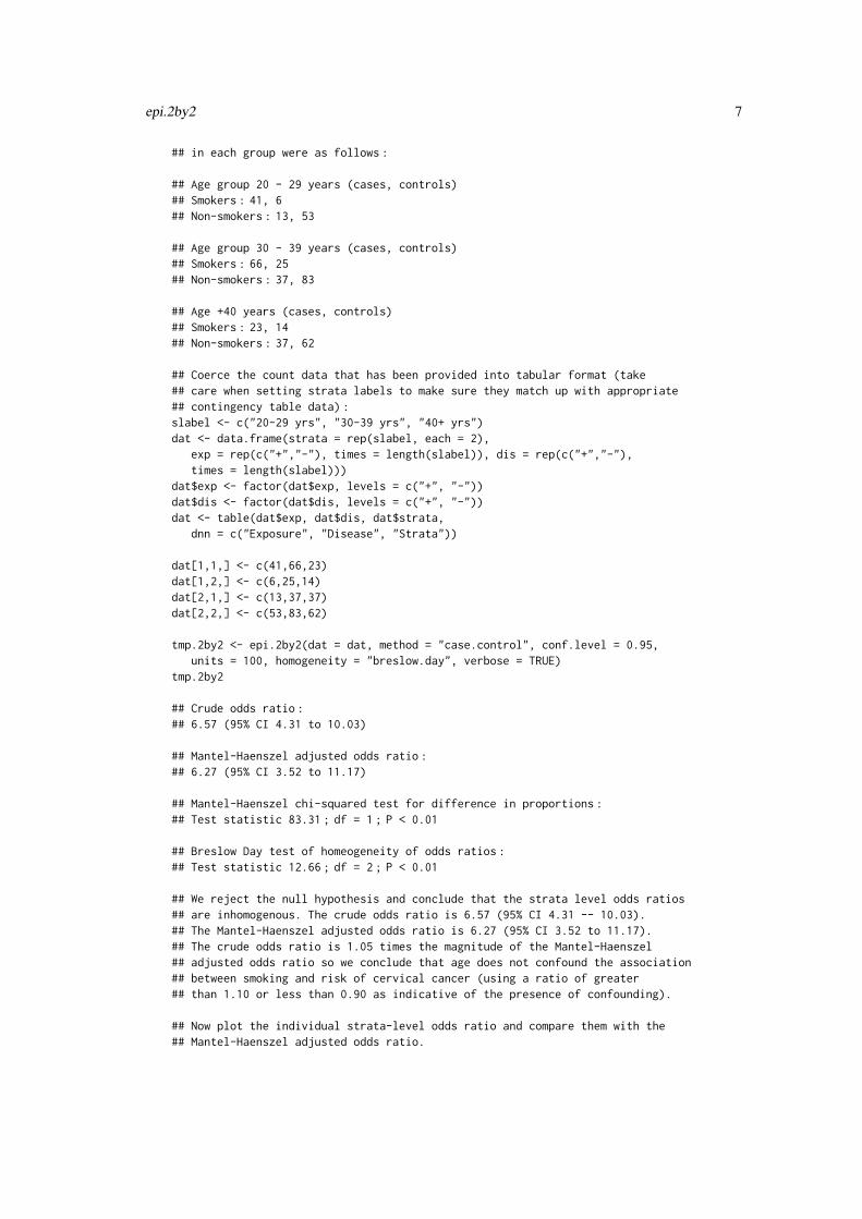
## We reject the null hypothesis and conclude that the strata level odds ratios## are inhomogenous. The crude odds ratio is 6.57 (95% CI 4.31 -- 10.03).## The Mantel-Haenszel adjusted odds ratio is 6.27 (95% CI 3.52 to 11.17).## The crude odds ratio is 1.05 times the magnitude of the Mantel-Haenszel## adjusted odds ratio so we conclude that age does not confound the association## between smoking and risk of cervical cancer (using a ratio of greater## than 1.10 or less than 0.90 as indicative of the presence of confounding).

## Now plot the individual strata-level odds ratio and compare them with the## Mantel-Haenszel adjusted odds ratio.

8 epi.about

## Not run:## Not run: library(latticeExtra)nstrata <- 1:dim(dat)[3]strata.lab <- paste("Strata ", nstrata, sep = "")y.at <- c(nstrata, max(nstrata) + 1)y.labels <- c("Mantel-Haenszel", strata.lab)x.labels <- c(0.5, 1, 2, 4, 8, 16, 32, 64, 128)

or.l <- c(tmp.2by2$OR.mh$lower, tmp.2by2$OR.strata$lower)or.u <- c(tmp.2by2$OR.mh$upper, tmp.2by2$OR.strata$upper)or.p <- c(tmp.2by2$OR.mh$est, tmp.2by2$OR.strata$est)vert <- 1:length(or.p)

segplot(vert ~ or.l + or.u, centers = or.p, horizontal = TRUE,aspect = 1/2, col = "grey",ylim = c(0,vert + 1),xlab = "Odds ratio", ylab = "",scales = list(y = list(at = y.at, labels = y.labels)),main = "Strata level and summary measures of association")

## End(Not run)## End(Not run)

## In this example the precision of both strata 2 and 3 odds ratio estimates is## high (i.e. the confidence intervals are narrow) so strata 2 and 3 carry most## of the weight in determining the value of the Mantel-Haenszel adjusted## odds ratio.

epi.about The library epiR: summary information

Description

An R package for the analysis of epidemiological data.

Usage

epi.about()

Details

The most recent version of the epiR package can be obtained from: http://epicentre.massey.ac.nz/

Author(s)

Mark Stevenson, EpiCentre, IVABS, Massey University, Palmerston North New Zealand.

Telmo Nunes, UISEE/DETSA, Faculdade de Medicina Veterinaria — UTL, Rua Prof. Cid dosSantos, 1300 - 477 Lisboa Portugal.

Javier Sanchez, Atlantic Veterinary College, University of Prince Edward Island, Charlottetown,Prince Edward Island, C1A 4P3, Canada.

Ron Thornton, MAF New Zealand, PO Box 2526 Wellington, New Zealand.

http://epicentre.massey.ac.nz/

http://epicentre.massey.ac.nz/

epi.bohning 9

epi.asc Write matrix to an ASCII raster file

Description

Writes a data frame to an ASCII raster file, suitable for display in ArcView or ArcGIS.

Usage

epi.asc(dat, file, xllcorner, yllcorner, cellsize, na = -9999)

Arguments

dat a matrix with data suitable for plotting using the image function.

file character string specifying the name and path of the ASCII raster output file.

xllcorner the easting coordinate corresponding to the lower left hand corner of the matrix.

yllcorner the northing coordinate corresponding to the lower left hand corner of the ma-trix.

cellsize number, defining the size of each matrix cell.

na scalar, defines null values in the matrix. NAs are converted to this value.

Value

Writes an ASCII raster file (typically with *.asc extension), suitable for display in a GIS package.

Note

The image function in R rotates tabular data counter clockwise by 90 degrees for display. A matrixof the form:

1 32 4

is displayed (using image) as:

3 41 2

It is recommended that the source data for this function is a matrix. Replacement of NAs in a dataframe extends processing time for this function.

epi.bohning Bohning’s test for overdispersion of Poisson data

10 epi.ccc

Description

A test for overdispersion of Poisson data.

Usage

epi.bohning(obs, exp, alpha = 0.05)

Arguments

obs the observed number of cases in each area.

exp the expected number of cases in each area.

alpha alpha level to be used for the test of significance. Must be a single numberbetween 0 and 1.

Value

A data frame with two elements: test.statistic, Bohning’s test statistic, p.value the associatedP-value.

References

Bohning D (2000). Computer-assisted Analysis of Mixtures and Applications. Chapman and Hall,Boca Raton.

Ugarte MD, Ibanez B, Militino AF (2006). Modelling risks in disease mapping. Statistical Methodsin Medical Research 15: 21 - 35.

Examples

data(epi.SClip)obs <- epi.SClip$casespop <- epi.SClip$populationexp <- (sum(obs) / sum(pop)) * pop

epi.bohning(obs, exp, alpha = 0.05)

epi.ccc Concordance correlation coefficient

Description

Calculates Lin’s (1989, 2000) concordance correlation coefficient for agreement on a continuousmeasure.

Usage

epi.ccc(x, y, ci = "z-transform", conf.level = 0.95)

epi.ccc 11

Arguments

x a vector, representing the first set of measurements.

y a vector, representing the second set of measurements.

ci a character string, indicating the method to be used. Options are z-transformor asymptotic.


Details

Computes Lin’s (1989, 2000) concordance correlation coefficient for agreement on a continuousmeasure obtained by two methods. The concordance correlation coefficient combines measures ofboth precision and accuracy to determine how far the observed data deviate from the line of perfectconcordance (that is, the line at 45 degrees on a square scatter plot). Lin’s coefficient increases invalue as a function of the nearness of the data’s reduced major axis to the line of perfect concordance(the accuracy of the data) and of the tightness of the data about its reduced major axis (the precisionof the data).

Both x and y values need to be present for a measurement pair to be included in the analysis. If eitheror both values are missing (i.e. coded NA) then the measurement pair is deleted before analysis.

Value

A list containing the following:

rho.c the concordance correlation coefficient.

s.shift the scale shift.

l.shift the location shift.

C.b a bias correction factor that measures how far the best-fit line deviates from aline at 45 degrees. No deviation from the 45 degree line occurs when C.b = 1.See Lin (1989, page 258).

blalt a data frame with two columns: mean the mean of each pair of measurements,delta vector y minus vector x.

nmissing a count of the number of measurement pairs ignored due to missingness.

References

Bland J, Altman D (1986). Statistical methods for assessing agreement between two methods ofclinical measurement. The Lancet 327: 307 - 310.

Bradley E, Blackwood L (1989). Comparing paired data: a simultaneous test for means and vari-ances. American Statistician 43: 234 - 235.

Dunn G (2004). Statistical Evaluation of Measurement Errors: Design and Analysis of ReliabilityStudies. London: Arnold.

Hsu C (1940). On samples from a normal bivariate population. Annals of Mathematical Statistics11: 410 - 426.

Krippendorff K (1970). Bivariate agreement coefficients for reliability of data. In: Borgatta E,Bohrnstedt G (eds) Sociological Methodology. San Francisco: Jossey-Bass, pp. 139 - 150.

Lin L (1989). A concordance correlation coefficient to evaluate reproducibility. Biometrics 45: 255- 268.

12 epi.ccc

Lin L (2000). A note on the concordance correlation coefficient. Biometrics 56: 324 - 325.

Pitman E (1939). A note on normal correlation. Biometrika 31: 9 - 12.

Reynolds M, Gregoire T (1991). Comment on Bradley and Blackwood. American Statistician 45:163 - 164.

Snedecor G, Cochran W (1989). Statistical Methods. Ames: Iowa State University Press.

Examples

## Concordance correlation plot:set.seed(seed = 1234)method1 <- rnorm(n = 100, mean = 0, sd = 1)method2 <- method1 + runif(n = 100, min = 0, max = 1)

## Introduce some missing values:method1[50] <- NAmethod2[75] <- NA

tmp.ccc <- epi.ccc(method1, method2, ci = "z-transform",conf.level = 0.95)

lab <- paste("CCC: ", round(tmp.ccc$rho.c[,1], digits = 2), " (95% CI ",round(tmp.ccc$rho.c[,2], digits = 2), " - ",round(tmp.ccc$rho.c[,3], digits = 2), ")", sep = "")

z <- lm(method2 ~ method1)

par(pty = "s")plot(method1, method2, xlim = c(0, 5), ylim = c(0,5), xlab = "Method 1",

ylab = "Method 2", pch = 16)abline(a = 0, b = 1, lty = 2)abline(z, lty = 1)legend(x = "topleft", legend = c("Line of perfect concordance",

"Reduced major axis"), lty = c(2,1), lwd = c(1,1), bty = "n")text(x = 1.55, y = 3.8, labels = lab)

## Bland and Altman plot (Figure 2 from Bland and Altman 1986):x <- c(494,395,516,434,476,557,413,442,650,433,417,656,267,

478,178,423,427)

y <- c(512,430,520,428,500,600,364,380,658,445,432,626,260,477,259,350,451)

tmp.ccc <- epi.ccc(x, y, ci = "z-transform", conf.level = 0.95)tmp.mean <- mean(tmp.ccc$blalt$delta)tmp.sd <- sqrt(var(tmp.ccc$blalt$delta))

plot(tmp.ccc$blalt$mean, tmp.ccc$blalt$delta, pch = 16,xlab = "Average PEFR by two meters (L/min)",ylab = "Difference in PEFR (L/min)", xlim = c(0,800),ylim = c(-140,140))

abline(h = tmp.mean, lty = 1, col = "gray")abline(h = tmp.mean - (2 * tmp.sd), lty = 2, col = "gray")abline(h = tmp.mean + (2 * tmp.sd), lty = 2, col = "gray")legend(x = "topleft", legend = c("Mean difference",

"Mean difference +/ 2SD"), lty = c(1,2), bty = "n")legend(x = 0, y = 125, legend = c("Difference"), pch = 16,

bty = "n")

epi.cluster1size 13

epi.cluster1size Sample size under under one-stage cluster sampling

Description

Returns the required number of clusters to be sampled using a one-stage cluster sampling strategy.

Usage

epi.cluster1size(n, mean, var, epsilon.r, method = "mean",conf.level = 0.95)

Arguments

n integer, representing the total number of clusters in the population.

mean number, representing the population mean of the variable of interest.

var number, representing the population variance of the variable of interest.

epsilon.r the maximum relative difference between our estimate and the unknown popu-lation value.

method a character string indicating the method to be used. Options are total, mean ormean.per.unit.

conf.level scalar, defining the level of confidence in the computed result.

Value

Returns an integer defining the required number of clusters to be sampled.

References

Levy PS, Lemeshow S (1999). Sampling of Populations Methods and Applications. Wiley Seriesin Probability and Statistics, London, pp. 258.

Examples

## We intend to conduct a survey of residents to estimate the total number## over 65 years of age that require the services of a nurse. There are## five housing complexes in the study area and we expect that there might## be a total of around 34 residents meeting this criteria (variance 6.8).## We would like the estimated sample size to provide us with an estimate## that is within 10% of the true value. How many housing complexes (clusters)## should be sampled?

epi.cluster1size(n = 5, mean = 34, var = 6.8, epsilon.r = 0.10, method ="total", conf.level = 0.999)

## We would need to sample 3 housing complexes to meet the specifications## for this study.

14 epi.cluster2size

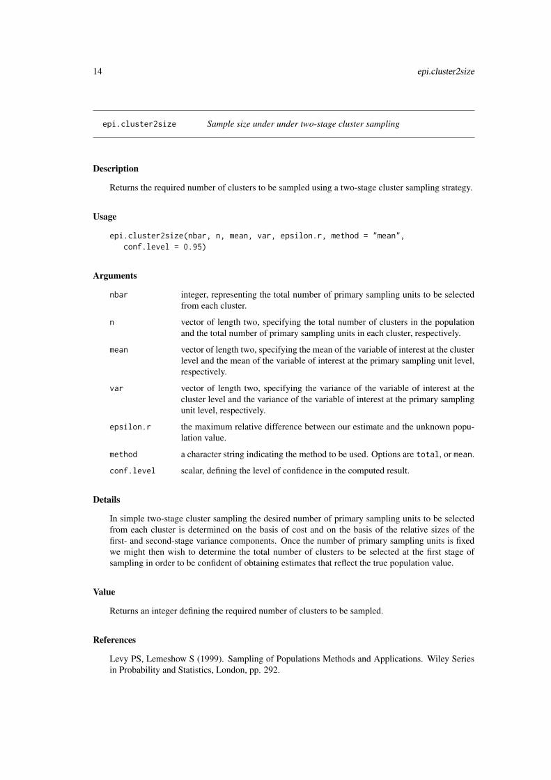
epi.cluster2size Sample size under under two-stage cluster sampling

Description

Returns the required number of clusters to be sampled using a two-stage cluster sampling strategy.

Usage

epi.cluster2size(nbar, n, mean, var, epsilon.r, method = "mean",conf.level = 0.95)

Arguments

nbar integer, representing the total number of primary sampling units to be selectedfrom each cluster.

n vector of length two, specifying the total number of clusters in the populationand the total number of primary sampling units in each cluster, respectively.

mean vector of length two, specifying the mean of the variable of interest at the clusterlevel and the mean of the variable of interest at the primary sampling unit level,respectively.

var vector of length two, specifying the variance of the variable of interest at thecluster level and the variance of the variable of interest at the primary samplingunit level, respectively.


method a character string indicating the method to be used. Options are total, or mean.


Details

In simple two-stage cluster sampling the desired number of primary sampling units to be selectedfrom each cluster is determined on the basis of cost and on the basis of the relative sizes of thefirst- and second-stage variance components. Once the number of primary sampling units is fixedwe might then wish to determine the total number of clusters to be selected at the first stage ofsampling in order to be confident of obtaining estimates that reflect the true population value.

Value

Returns an integer defining the required number of clusters to be sampled.

References

Levy PS, Lemeshow S (1999). Sampling of Populations Methods and Applications. Wiley Seriesin Probability and Statistics, London, pp. 292.

epi.clustersize 15

Examples

## We intend to conduct a survey of nurse practitioners to estimate the## average number of patients seen by each nurse. There are five health## centres in the study area, each with three nurses. We intend to sample## two nurses from each health centre. We would like to be 95% confident## of obtaining an estimate that is within 30% of the true population value.## We expect that the mean number of patients seen at the health centre level## is 84 (var 567) and the mean number of patients seen at the nurse## level is 28 (var 160). How many health centres should we sample?

nbar <- 2; n <- c(5, 3); mean <- c(84, 28); var <- c(567, 160)epi.cluster2size(nbar, n, mean, var, epsilon.r = 0.3, method = "mean",

conf.level = 0.95)

## We would need a simple two-stage cluster sample of 3 health centres to## meet these specifications.

epi.clustersize Sample size for cluster-sample surveys

Description

Estimates the number of clusters to be sampled using a cluster-sample design.

Usage

epi.clustersize(p, b, rho, epsilon, conf.level = 0.95)

Arguments

p the estimated prevalence of disease in the population.b the number of units to be sampled per cluster.rho the intra-cluster correlation, a measure of the variation between clusters com-

pared with the variation within clusters.epsilon scalar, the acceptable absolute error.conf.level scalar, defining the level of confidence in the computed result.

Value


clusters the estimated number of clusters to be sampled.units the total number of units to be sampled.design the design effect.

Note

The intra-cluster correlation (rho) will be higher for those situations where the between-clustervariation is greater than within-cluster variation. The design effect is dependent on rho and b (thenumber of units sampled per cluster): rho = (D - 1) / (b - 1). Design effects of 2, 4, and 7can be used to estimate rho when intra-cluster correlation is low, medium, and high (respectively).A design effect of 7.5 should be used when the intra-cluster correlation is unknown.

16 epi.conf

References

Otte J, Gumm I (1997). Intra-cluster correlation coefficients of 20 infections calculated from theresults of cluster-sample surveys. Preventive Veterinary Medicine 31: 147 - 150.

Bennett S, Woods T, Liyanage WM, Smith DL (1991). A simplified general method for cluster-sample surveys of health in developing countries. Raport trimestriel de statistiques sanitaires modi-ales 44: 98 - 106.

Examples

## The expected prevalence of disease in a population of cattle is 0.10.## We wish to conduct a survey, sampling 50 animals per farm. No data## are available to provide an estimate of rho, though we suspect## the intra-cluster correlation for this disease to be relatively high.## We wish to be 95% certain of being within 10% of the true population## prevalence of disease. How many herds should be sampled?

p <- 0.10b <- 50D <- 7rho <- (D - 1) / (b - 1)epi.clustersize(p = 0.10, b = 50, rho = rho, epsilon = 0.10, conf.level = 0.95)

## We need to sample 485 herds (24250 samples in total).

epi.conf Confidence intervals for means, proportions, incidence, and standard-ised mortality ratios

Description

Computes confidence intervals for means, proportions, incidence, and standardised mortality ratios.

Usage

epi.conf(dat, ctype = "mean.single", method, N, design = 1,conf.level = 0.95)

Arguments

dat the data, either a vector or a matrix depending on the method chosen.

ctype a character string indicating the type of confidence interval to calculate. Optionsare mean.single, mean.unpaired, mean.paired, prop.single, prop.unpaired,prop.paired, prevalence, inc.risk, inc.rate, and smr.

method a character string indicating the method to use. Where ctype = "inc.risk"or ctype = "prevalence" options are exact, wilson and fleiss. Wherectype = "inc.rate" options are exact and byar.

N scalar, representing the population size.

design scalar, representing the design effect.


epi.conf 17

Details

Method mean.single requires a vector as input. Method mean.unpaired requires a two-columndata frame; the first column defining the groups must be a factor. Method mean.paired requires atwo-column data frame; one column for each group. Method prop.single requires a two-columnmatrix; the first column specifies the number of positives, the second column specifies the numberof negatives. Methods prop.unpaired and prop.paired require a four-column matrix; columns1 and 2 specify the number of positives and negatives for the first group, columns 3 and 4 specifythe number of positives and negatives for the second group. Method prevalence and inc.riskrequire a two-column matrix; the first column specifies the number of positives, the second columnspecifies the total number tested. Method inc.rate requires a two-column matrix; the first columnspecifies the number of positives, the second column specifies individual time at risk. Method smrrequires a two-colum matrix; the first column specifies the total number of positives, the secondcolumn specifies the total number tested.

The methodology implemented here follows Altman, Machin, Bryant, and Gardner (2000). Wheremethod is inc.risk, prevalence or inc.rate if the numerator equals zero the lower bound ofthe confidence interval estimate is set to zero. Where method is smr the method of Dobson et al.(1991) is used. A summary of the methods used for each of the confidence interval calculations isas follows:

ctype-method Referencemean.single Altman et al. (2000)mean.unpaired Altman et al. (2000)mean.paired Altman et al. (2000)prop.single Altman et al. (2000)prop.unpaired Altman et al. (2000)prop.paired Altman et al. (2000)inc.risk, exact Collett (1999)inc.risk, wilson Rothman (2002)inc.risk, fleiss Fleiss (1981)prevalence, exact Collett (1999)prevalence, wilson Rothman (2002)prevalence, fleiss Fleiss (1981)inc.rate, exact Collett (1999)inc.rate, byar Rothman (2002)smr Dobson et al. (1991)

The design effect is used to adjust the confidence interval around a prevalence or incidence riskestimate in the presence of clustering. The design effect is a measure of the variability betweenclusters and is calculated as the ratio of the variance calculated assuming a complex sample designdivided by the variance calculated assuming simple random sampling. Adjustment for the effect ofclustering can only be done on those prevalence and incidence risk methods that return a standarderror (i.e. method = "wilson" or method = "fleiss").

References

Altman DG, Machin D, Bryant TN, and Gardner MJ (2000). Statistics with Confidence, secondedition. British Medical Journal, London, pp. 28 - 29 and pp. 45 - 56.

Collett D (1999). Modelling Binary Data. Chapman & Hall/CRC, Boca Raton Florida, p. 24.

Dobson AJ, Kuulasmaa K, Eberle E, and Scherer J (1991). Confidence intervals for weighted sumsof Poisson parameters. Statistics in Medicine 10: 457 - 462.

18 epi.conf

Fleiss JL (1981). Statistical Methods for Rates and Proportions. 2nd edition. John Wiley & Sons,New York.

Killip S, Mahfoud Z, Pearce K (2004). What is an intracluster correlation coefficient? Crucialconcepts for primary care researchers. Annals of Family Medicine 2: 204 - 208.


Rothman KJ (2002). Epidemiology An Introduction. Oxford University Press, London, pp. 130 -143.

Examples

## EXAMPLE 1dat <- rnorm(n = 100, mean = 0, sd = 1)epi.conf(dat, ctype = "mean.single")

## EXAMPLE 2group <- c(rep("A", times = 5), rep("B", times = 5))val = round(c(rnorm(n = 5, mean = 10, sd = 5),

rnorm(n = 5, mean = 7, sd = 5)), digits = 0)dat <- data.frame(group = group, val = val)epi.conf(dat, ctype = "mean.unpaired")

## EXAMPLE 3## Two paired samples (Altman et al. 2000, page 31):## Systolic blood pressure levels were measured in 16 middle-aged men## before and after a standard exercise test. The mean rise in systolic## blood pressure was 6.6 mmHg. The standard deviation of the difference## was 6.0 mm Hg. The standard error of the mean difference was 1.49 mm Hg.

before <- c(148,142,136,134,138,140,132,144,128,170,162,150,138,154,126,116)after <- c(152,152,134,148,144,136,144,150,146,174,162,162,146,156,132,126)dat <- data.frame(before, after)dat <- data.frame(cbind(before, after))epi.conf(dat, ctype = "mean.paired", conf.level = 0.95)

## The 95% confidence interval for the population value of the mean## systolic blood pressure increase after standard exercise was 3.4 to 9.8## mm Hg.

## EXAMPLE 4## Single sample (Altman et al. 2000, page 47):## Out of 263 giving their views on the use of personal computers in## general practice, 81 thought that the privacy of their medical file## had been reduced.

pos <- 81neg <- (263 - 81)dat <- as.matrix(cbind(pos, neg))round(epi.conf(dat, ctype = "prop.single"), digits = 3)

## The 95% confidence interval for the population value of the proportion## of patients thinking their privacy was reduced was from 0.255 to 0.366.

## EXAMPLE 5## Two samples, unpaired (Altman et al. 2000, page 49):## Goodfield et al. report adverse effects in 85 patients receiving either

epi.conf 19

## terbinafine or placebo treatment for dermatophyte onchomychois.## Out of 56 patients receiving terbinafine, 5 patients experienced## adverse effects. Out of 29 patients receiving a placebo, none experienced## adverse effects.

grp1 <- matrix(cbind(5, 51), ncol = 2)grp2 <- matrix(cbind(0, 29), ncol = 2)dat <- as.matrix(cbind(grp1, grp2))round(epi.conf(dat, ctype = "prop.unpaired"), digits = 3)

## The 95% confidence interval for the difference between the two groups is## from -0.038 to +0.193.

## EXAMPLE 6## Two samples, paired (Altman et al. 2000, page 53):## In a reliability exercise, 41 patients were randomly selected from those## who had undergone a thalium-201 stress test. The 41 sets of images were## classified as normal or not by the core thalium laboratory and,## independently, by clinical investigators from different centres.## Of the 19 samples identified as ischaemic by clinical investigators## 5 were identified as ischaemic by the laboratory. Of the 22 samples## identified as normal by clinical investigators 0 were identified as## ischaemic by the laboratory.

## Clinic | Laboratory | |## | Ischaemic | Normal | Total## ---------------------------------------------------------## Ischaemic | 14 | 5 | 19## Normal | 0 | 22 | 22## ---------------------------------------------------------## Total | 14 | 27 | 41## ---------------------------------------------------------

dat <- as.matrix(cbind(14, 5, 0, 22))round(epi.conf(dat, ctype = "prop.paired", conf.level = 0.95), digits = 3)

## The 95% confidence interval for the population difference in## proportions is 0.011 to 0.226 or approximately +1% to +23%.

## EXAMPLE 7## A herd of 1000 cattle were tested for brucellosis. Two samples out of 200## test returned a positive result. Assuming 100% test sensitivity and## specificity, what is the estimated prevalence of brucellosis in this## group of animals?

pos <- 4; pop <- 200dat <- as.matrix(cbind(pos, pop))epi.conf(dat, ctype = "prevalence", method = "exact", N = 1000,

design = 1, conf.level = 0.95) * 100

## The estimated prevalence of brucellosis in this herd is 2 cases## per 100 cattle (95% CI 0.54 -- 5.0 cases per 100 cattle).

## EXAMPLE 8## The observed disease counts and population size in four areas are provided## below. What are the the standardised morbidity ratios of disease for each## area and their 95% confidence intervals?

20 epi.convgrid

obs <- c(5, 10, 12, 18); pop <- c(234, 189, 432, 812)dat <- as.matrix(cbind(obs, pop))round(epi.conf(dat, ctype = "smr"), digits = 2)

## EXAMPLE 9## A survey has been conducted to determine the proportion of broilers## protected from a given disease following vaccination. We assume that## the intra-cluster correlation coefficient for protection (also known as the## rate of homogeneity, rho) is 0.4 and the average number of birds per## flock is 30. A total of 5898 birds from a total of 10363 were identified## as protected. What proportion of birds are protected and what is the 95%## confidence interval for this estimate?

## Calculate the design effect, given rho = (design - 1) / (nbar - 1), where## nbar equals the average number of individuals per cluster:

design <- 0.4 * (30 - 1) + 1

## The design effect is 12.6. Now calculate the proportion protected:

dat <- as.matrix(cbind(5898, 10363))epi.conf(dat, ctype = "prevalence", method = "fleiss", N = 1000000,

design = design, conf.level = 0.95)

## The estimated proportion of the population protected is 0.57 (95% CI## 0.53 -- 0.60). If we had mistakenly assumed that data were a simple random## sample the confidence interval would have been 0.56 -- 0.58.

epi.convgrid Convert British National Grid georeferences to easting and northingcoordinates

Description

Convert British National Grid georeferences to easting and northing coordinates.

Usage

epi.convgrid(os.refs)

Arguments

os.refs a vector of character strings listing the British National Grid georeferences to beconverted.

Note

If an invalid georeference is encountered in the vector os.ref the method returns a NA.

epi.cp 21

Examples

os.refs <- c("SJ505585","SJ488573","SJ652636")epi.convgrid(os.refs)

epi.cp Extract unique covariate patterns from a data set

Description

Extract the set of unique patterns from a set of covariates.

Usage

epi.cp(dat)

Arguments

dat an i row by j column data frame where the i rows represent individual observa-tions and the m columns represent covariates.

Details

A covariate pattern is a unique combination of values of predictor variables. For example, if a modelcontains two dichotomous predictors, there will be four covariate patterns possible: (1,1), (1,0),(0,1), and (0,0). This function extracts the n unique covariate patterns from a data set comprisedof i observations, labelling them from 1 to n. A vector of length m is also returned, listing thecovariate pattern identifier for each observation.

Value


cov.pattern a data frame with columns: id the unique covariate patterns, n the number ofoccasions each of the listed covariate pattern appears in the data, and the uniquecovariate combinations.

id a vector listing the covariate pattern identifier for each observation.

References

Dohoo I, Martin W, Stryhn H (2003). Veterinary Epidemiologic Research. AVC Inc, Charlottetown,Prince Edward Island, Canada.

Examples

## Generate a set of covariates:set.seed(seed = 1234)obs <- round(runif(n = 100, min = 0, max = 1), digits = 0)v1 <- round(runif(n = 100, min = 0, max = 4), digits = 0)v2 <- round(runif(n = 100, min = 0, max = 4), digits = 0)dat <- as.data.frame(cbind(obs, v1, v2))

22 epi.cpresids

dat.glm <- glm(obs ~ v1 + v2, family = binomial, data = dat)dat.mf <- model.frame(dat.glm)

## Covariate pattern:epi.cp(dat.mf[-1])

## There are 25 covariate patterns in this data set. Subject 100 has## covariate pattern 21.

epi.cpresids Covariate pattern residuals from a logistic regression model

Description

Returns covariate pattern residuals and delta betas from a logistic regression model.

Usage

epi.cpresids(obs, fit, covpattern)

Arguments

obs a vector of observed values (i.e. counts of ‘successes’) for each covariate pat-tern).

fit a vector defining the predicted (i.e. fitted) probability of success for each covari-ate pattern.

covpattern a epi.cp object.

Value

A data frame with 13 elements: cpid the covariate pattern identifier, n the number of subjects inthis covariate pattern, obs the observed number of successes, pred the predicted number of suc-cesses, raw the raw residuals, sraw the standardised raw residuals, pearson the Pearson residuals,spearson the standardised Pearson residuals, deviance the deviance residuals, leverage lever-age, deltabeta the delta-betas, sdeltabeta the standardised delta-betas, and deltachi delta chistatistics.

References

Hosmer DW, Lemeshow S (1989). Applied Logistic Regression. John Wiley & Sons, New York,USA, pp. 137 - 138.

See Also

epi.cp

epi.descriptives 23

Examples

infert.glm <- glm(case ~ spontaneous + induced, data = infert,family = binomial())

infert.mf <- model.frame(infert.glm)infert.cp <- epi.cp(infert.mf[-1])

infert.obs <- as.vector(by(infert$case, as.factor(infert.cp$id),FUN = sum))

infert.fit <- as.vector(by(fitted(infert.glm), as.factor(infert.cp$id),FUN = min))

infert.res <- epi.cpresids(obs = infert.obs, fit = infert.fit,covpattern = infert.cp)

epi.descriptives Descriptive statistics

Description

Computes descriptive statistics from a vector of numbers.

Usage

epi.descriptives(dat, quantile = c(0.025, 0.975))

Arguments

dat vector for which descriptive statistics will be calculated.

quantile vector of length two specifying quantiles to be calculated.

Examples

tmp <- rnorm(1000, mean = 0, sd = 1)epi.descriptives(tmp, quantile = c(0.025, 0.975))

epi.detectsize Sample size to detect disease

Description

Estimates the required sample size to detect disease. The method adjusts sample size estimates onthe basis of test sensitivity and specificity and can account for series and parallel test interpretation.

Usage

epi.detectsize(N, prev, se, sp, interpretation = "series",covar = c(0,0), conf.level = 0.95, finite.correction = TRUE)

24 epi.detectsize

Arguments

N a vector of length one or two defining the size of the population. The first ele-ment of the vector defines the number of clusters, the second element definingthe mean number of sampling units per cluster.

prev a vector of length one or two defining the prevalence of disease in the popula-tion. The first element of the vector defines the between-cluster prevalence, thesecond element defines the within-cluster prevalence.

se a vector of length one or two defining the sensitivity of the test(s) used.

sp a vector of length one or two defining the specificity of the test(s) used.

interpretation a character string indicating how test results should be interpreted. Options areseries or parallel.

covar a vector of length two defining the covariance between test results for diseasepositive and disease negative groups. The first element of the vector is the co-variance between test results for disease positive subjects. The second elementof the vector is the covariance between test results for disease negative subjects.Use covar = c(0,0) (the default) if these values are not known.

conf.level scalar, defining the level of confidence in the computed result.finite.correction

logial, should a finite correction factor be applied?

Value


performance The sensitivity and specificity of the testing strategy.

sample.size The number of clusters, units, and total number of units to be sampled.

Note

The finite correction factor reduces the variance of the sample as the sample size approaches thepopulation size. As a rule of thumb, set finite.correction = TRUE when the sample size isgreater than 5% of the population size.

Define se1 and se2 as the sensitivity for the first and second test, sp1 and sp2 as the specificity forthe first and second test, p111 as the proportion of disease-positive subjects with a positive test resultto both tests and p000 as the proportion of disease-negative subjects with a negative test result toboth tests. The covariance between test results for the disease-positive group is p111 - se1 * se2.The covariance between test results for the disease-negative group is p000 - sp1 * sp2.

References

Dohoo I, Martin W, Stryhn H (2003). Veterinary Epidemiologic Research. AVC Inc, Charlottetown,Prince Edward Island, Canada, pp. 47 and pp 102 - 103.

Examples

## EXAMPLE 1## We would like to confirm the absence of disease in a single 1000-cow## dairy herd. We expect the prevalence of disease in the herd to be 5%.## We intend to use a single test with a sensitivity of 0.90 and a## specificity of 0.80. How many samples should we take to be 95% certain## that, if all tests are negative, the disease is not present?

epi.dgamma 25

epi.detectsize(N = 1000, prev = 0.05, se = 0.90, sp = 0.80, interpretation ="series", covar = c(0,0), conf.level = 0.95, finite.correction = TRUE)

## We need to sample 59 cows.

## EXAMPLE 2## We would like to confirm the absence of disease in a study area. If the## disease is present we expect the between-herd prevalence to be 8% and the## within-herd prevalence to be 5%. We intend to use two tests: the first has## a sensitivity and specificity of 0.90 and 0.80, respectively. The second## has a sensitivity and specificity of 0.95 and 0.85, respectively. The two## tests will be interpreted in parallel. How many herds and cows within herds## should we sample to be 95% certain that the disease is not present in the## study area if all tests are negative? There area is comprised of## approximately 5000 herds and the average number of cows per herd is 100.

epi.detectsize(N = c(5000, 100), prev = c(0.08, 0.05), se = c(0.90, 0.95),sp = c(0.80, 0.85), interpretation = "parallel", covar = c(0,0),conf.level = 0.95, finite.correction = TRUE)

## We need to sample 31 cows from 38 herds (a total of 1178 samples).## The sensitivity of this testing regime is 99%. The specificity of this## testing regime is 68%.

## EXAMPLE 3## You want to document the absence of Mycoplasma from a 200-sow pig herd.## Based on your experience and the literature, a minimum of 20% of sows## would have seroconverted if Mycoplasma were present in the herd. How many## sows do you need to sample?

epi.detectsize(N = 200, prev = 0.20, se = 1.00, sp = 1.00, conf.level = 0.95,finite.correction = TRUE)

## If you test 12 sows and all test negative you can state that you are 95%## confident that the prevalence rate of Mycoplasma in the herd is less than## 20%.

epi.dgamma Estimate the precision of a [structured] heterogeneity term

Description

Returns the precision of a [structured] heterogeneity term after one has specified the amount ofvariation a priori.

Usage

epi.dgamma(rr, quantiles = c(0.05, 0.95))

Arguments

rr the lower and upper limits of relative risk, estimated a priori.

26 epi.directadj

quantiles a vector of length two defining the quantiles of the lower and upper relative riskestimates.

Value

Returns the precision (the inverse variance) of the heterogeneity term.

References

Best, NG. WinBUGS 1.3.1 Short Course, Brisbane, November 2000.

Examples

## Suppose we are expecting the lower 5% and upper 95% confidence interval## of relative risk in a data set to be 0.5 and 3.0, respectively.## A prior guess at the precision of the heterogeneity term would be:

tau <- epi.dgamma(rr = c(0.5, 3.0), quantiles = c(0.05, 0.95))tau

## This can be translated into a gamma distribution. We set the mean of the## distribution as tau and specify a large variance (that is, we are not## certain about tau).

mean <- tauvar <- 1000shape <- mean^2 / varinv.scale <- mean / var

## In WinBUGS the precision of the heterogeneity term may be parameterised## as tau ~ dgamma(shape, inv.scale). Plot the probability density function## of tau:

z <- seq(0.01, 10, by = 0.01)fz <- dgamma(z, shape = shape, scale = 1/inv.scale)plot(z, fz, type = "l", ylab = "Probability density of tau")

epi.directadj Directly adjusted incidence risk estimates

Description

Compute directly adjusted incidence risks.

Usage

epi.directadj(obs, pop, std, units = 1, conf.level = 0.95)

epi.directadj 27

Arguments

obs a matrix representing the observed number of events. Rows represent strata(e.g. region); columns represent the covariates to be adjusted for (e.g. age class,gender). The sum of each row will equal the total number of events for eachstratum. If there are no covariates to be adjusted for obs will be a one columnmatrix. The dimensions of the obs matrix must be named (see the examples,below).

pop a matrix representing population size. Rows represent strata (e.g. region);columns represent the covariates to be adjusted for (e.g. age class, gender).The sum of each row will equal the total population size within each stratum. Ifthere are no covariates pop will be a one column matrix. The dimensions of thepop matrix must be named (see the examples, below).

std a matrix representing the standard population size for the different levels of thecovariate to be adjusted for.

units multiplier for the incidence risk estimates.


Details

This function returns unadjusted (crude) and directly adjusted incidence risk estimates for each ofthe specified population strata. The term ‘covariate’ is used here to refer to the factors we want tocontrol (i.e. adjust) for when calculating the directly adjusted incidence risk estimates.

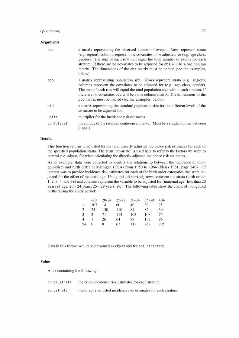
As an example, data were collected to identify the relationship between the incidence of mon-goloidism and birth order in Michigan (USA) from 1950 to 1964 (Fleiss 1981, page 240). Ofinterest was to provide incidence risk estimates for each of the birth order categories that were ad-justed for the effect of maternal age. Using epi.directadj rows represent the strata (birth order:1, 2, 3, 4, and 5+) and columns represent the variable to be adjusted for (maternal age: less than 20years of age, 20 - 24 years, 25 - 29 years, etc). The following table show the count of mongoloidbirths during the study period:

-20 20-24 25-29 30-34 35-39 40+1 107 141 60 40 39 252 25 150 110 84 82 393 3 71 114 103 108 754 1 26 64 89 137 965+ 0 8 63 112 262 295

Data in this format would be presented as object obs for epi.directadj.

Value


crude.strata the crude incidence risk estimates for each stratum.

adj.strata the directly adjusted incidence risk estimates for each stratum.

28 epi.dms

References

Fay M, Feuer E (1997). Confidence intervals for directly standardized rates: A method based onthe gamma distribution. Statistics in Medicine 16: 791 - 801.

Fleiss JL (1981). Statistical Methods for Rates and Proportions, Wiley, New York, USA.

Greenland S, Rothman KJ. Introduction to stratified analysis. In: Rothman KJ, Greenland S (1998).Modern Epidemiology. Lippincott Williams, & Wilkins, Philadelphia, pp. 260 - 265.

See Also

epi.indirectadj

Examples

## A study was conducted to estimate the seroprevalence of leptospirosis## in dogs in Glasgow and Edinburgh, Scotland. The following data were## obtained for male and female dogs:

obs <- matrix(data = c(15,46,53,16), nrow = 2, byrow = TRUE,dimnames = list(c("ED","GL"), c("M","F")))

pop <- matrix(data = c(48,212,180,71), nrow = 2, byrow = TRUE,dimnames = list(c("ED","GL"), c("M","F")))

## Compute directly adjusted seroprevalence estimates, using a standard## population with equal numbers of male and female dogs:

std <- matrix(data = c(250,250), nrow = 1, byrow = TRUE,dimnames = list("", c("M","F")))

epi.directadj(obs, pop, std, units = 1, conf.level = 0.95)

## > $crude.strata## > est lower upper## > ED 0.2346154 0.1794622 0.3013733## > GL 0.2749004 0.2138889 0.3479040

## > $adj.strata## > est lower upper## > ED 0.2647406 0.1866047 0.3692766## > GL 0.2598983 0.1964162 0.3406224

## The confounding effect of sex has been removed by the gender-adjusted## incidence risk estimates.

epi.dms Decimal degrees and degrees, minutes and seconds conversion

Description

Converts decimal degrees to degrees, minutes and seconds. Converts degrees, minutes and secondsto decimal degrees.

epi.dsl 29

Usage

epi.dms(dat)

Arguments

dat the data. A one-column matrix is assumed when converting decimal degrees todegrees, minutes, and seconds. A two-column matrix is assumed when convert-ing degrees and decimal minutes to decimal degrees. A three-column matrix isassumed when converting degrees, minutes and seconds to decimal degrees.

Examples

## EXAMPLE 1 Degrees, minutes, seconds to decimal degrees:dat <- matrix(c(41, 38, 7.836, -40, 40, 27.921),

byrow = TRUE, nrow = 2)epi.dms(dat)

## EXAMPLE 2 Decimal degrees to degrees, minutes, secondsdat <- matrix(c(41.63551, -40.67442), nrow = 2)epi.dms(dat)

epi.dsl Mixed-effects meta-analysis of binary outcomes using the DerSimo-nian and Laird method

Description

Computes individual study odds or risk ratios for binary outcome data. Computes the summaryodds or risk ratio using the DerSimonian and Laird method. Performs a test of heterogeneity amongtrials. Performs a test for the overall difference between groups (that is, after pooling the studies,do treated groups differ significantly from controls?).

Usage

epi.dsl(ev.trt, n.trt, ev.ctrl, n.ctrl, names, method = "odds.ratio",alternative = c("two.sided", "less", "greater"), conf.level = 0.95)

Arguments

ev.trt observed number of events in the treatment group.

n.trt number in the treatment group.

ev.ctrl observed number of events in the control group.

n.ctrl number in the control group.

names character string identifying each trial.

method a character string indicating the method to be used. Options are odds.ratio orrisk.ratio.

alternative a character string specifying the alternative hypothesis, must be one of two.sided,greater or less.


30 epi.dsl

Details

alternative = "greater" tests the hypothesis that the DerSimonian and Laird summary measureof association is greater than 1.

Value


OR the odds ratio for each trial, the standard error of the odds ratio for each trial,and the lower and upper bounds of the confidence interval of the odds ratio foreach trial.

RR the risk ratio for each trial, the standard error of the risk ratio for each trial, andthe lower and upper bounds of the confidence interval of the risk ratio for eachtrial.

OR.summary the DerSimonian and Laird summary odds ratio, the standard error of the Der-Simonian and Laird summary odds ratio, the lower and upper bounds of theconfidence interval of the DerSimonian and Laird summary odds ratio.

RR.summary the DerSimonian and Laird summary risk ratio, the standard error of the DerSi-monian and Laird summary risk ratio, the lower and upper bounds of the confi-dence interval of the DerSimonian and Laird summary risk ratio.

weights the inverse variance and DerSimonian and Laird weights for each trial.

heterogeneity a vector containing Q the heterogeneity test statistic, df the degrees of freedomand its associated P-value.

Hsq the relative excess of the heterogeneity test statistic Q over the degrees of free-dom df.

Isq the percentage of total variation in study estimates that is due to heterogeneityrather than chance.

tau.sq the variance of the treatment effect among trials.

effect a vector containing z the test statistic for overall treatment effect and its associ-ated P-value.

Note

Under the random-effects model, the assumption of a common treatment effect is relaxed, and theeffect sizes are assumed to have a normal distribution with variance tau.sq.

Using this method, the DerSimonian and Laird weights are used to compute the pooled odds ratio.


References

Deeks JJ, Altman DG, Bradburn MJ (2001). Statistical methods for examining heterogeneity andcombining results from several studies in meta-analysis. In: Egger M, Davey Smith G, AltmanD (eds). Systematic Review in Health Care Meta-Analysis in Context. British Medical Journal,London, 2001, pp. 291 - 299.

DerSimonian R, Laird N (1986). Meta-analysis in clinical trials. Controlled Clinical Trials 7: 177- 188.

Higgins J, Thompson S (2002). Quantifying heterogeneity in a meta-analysis. Statistics in Medicine21: 1539 - 1558.

epi.edr 31

See Also

epi.iv, epi.mh, epi.smd

Examples

data(epi.epidural)epi.dsl(ev.trt = epi.epidural$ev.trt, n.trt = epi.epidural$n.trt,

ev.ctrl = epi.epidural$ev.ctrl, n.ctrl = epi.epidural$n.ctrl,names = as.character(epi.epidural$trial), method = "odds.ratio",alternative = "two.sided", conf.level = 0.95)

epi.edr Estimated dissemination ratio

Description

Computes estimated dissemination ratio on the basis of a vector of numbers (usually counts ofincident cases identified on each day of an epidemic).

Usage

epi.edr(dat, n = 4, conf.level = 0.95, nsim = 99, na.zero = TRUE)

Arguments

dat a numeric vector listing the number of incident cases for each day of an epi-demic.

n scalar, defining the number of days to be used when computing the estimateddissemination ratio.


nsim scalar, defining the number of simulations to be used for the confidence intervalcalculations.

na.zero logical, replace NaN or Inf values with zeros?

Details

In infectious disease epidemics the n-day estimated dissemination ratio (EDR) at day i equals thetotal number of incident cases between day i and day [i - (n - 1)] (inclusive) divided by thetotal number of incident cases between day (i - n) and day (i - 2n) + 1 (inclusive). EDRvalues are often calculated for each day of an epidemic and presented as a time series analysis. Ifthe EDR is consistently less than unity, the epidemic is said to be ‘under control.’

A simulation approach is used to calculate confidence intervals around each daily EDR estimate.The numerator and denominator of the EDR estimate for each day is taken in turn and a randomnumber drawn from a Poisson distribution, using the calculated numerator and denominator valueas the mean. EDR is then calculated for these simulated values and the process repeated nsim times.Confidence intervals are then derived from the vector of simulated values for each day.

32 epi.empbayes

Value

Returns the point estimate of the EDR and the lower and upper bounds of the confidence interval ofthe EDR.

Examples

set.seed(123)dat <- rpois(n = 50, lambda = 2)edr.04 <- epi.edr(dat, n = 4, conf.level = 0.95, nsim = 99, na.zero = TRUE)

## Plot:plot(1:50, 1:50, xlim = c(0,25), ylim = c(0, 10), xlab = "Days",

ylab = "Estimated dissemination ratio", type = "n", main = "")lines(1:50, edr.04[,1], type = "l", lwd = 2, lty = 1, col = "blue")lines(1:50, edr.04[,2], type = "l", lwd = 1, lty = 2, col = "blue")lines(1:50, edr.04[,3], type = "l", lwd = 1, lty = 2, col = "blue")

epi.empbayes Empirical Bayes estimates

Description

Computes empirical Bayes estimates of observed event counts using the method of moments.

Usage

epi.empbayes(obs, pop)

Arguments

obs a vector representing the observed disease counts in each region of interest.pop a vector representing the population count in each region of interest.

Details

The gamma distribution is sometimes parameterised in terms of shape and rate parameters. The rateparameter equals the inverse of the scale parameter. The mean of the distribution equals δ/α. Thevariance of the distribution equals δ/α2. The empirical Bayes estimate of the proportion affected ineach area equals (obs+ δ)/(pop+ α).

Value

A data frame with four elements: gamma mean observed event count, phi variance of observedevent count, alpha shape parameter of gamma distribution, and delta scale parameter of gammadistribution.

References

Bailey TC, Gatrell AC (1995). Interactive Spatial Data Analysis. Longman Scientific & Technical.London.

Langford IH (1994). Using empirical Bayes estimates in the geographical analysis of disease risk.Area 26: 142 - 149.

epi.epidural 33

Examples

data(epi.SClip)obs <- epi.SClip$casespop <- epi.SClip$population

est <- epi.empbayes(obs, pop)empbayes.prop <- (obs + est[4]) / (pop + est[3])raw.prop <- (obs) / (pop)rank <- rank(raw.prop)dat <- as.data.frame(cbind(rank, raw.prop, empbayes.prop))

plot(dat$rank, dat$raw.prop, type = "n", xlab = "Rank", ylab = "Proportion")points(dat$rank, dat$raw.prop, pch = 16, col = "red")points(dat$rank, dat$empbayes.prop, pch = 16, col = "blue")legend(5, 0.00025, legend = c("Raw estimate", "Bayes adjusted estimate"),

col = c("red","blue"), pch = c(16,16), bty = "n")

epi.epidural Rates of use of epidural anaesthesia in trials of caregiver support

Description

This data set provides results of six trials investigating rates of use of epidural anaesthesia duringchildbirth. Each trial is made up of a group where a caregiver (midwife, nurse) provided supportintervention and a group where standard care was provided. The objective was to determine if therewere higher rates of epidural use when a caregiver was present at birth.

Usage

data(epi.epidural)

Format

A data frame with 6 observations on the following 5 variables.

trial the name and year of the trial.

ev.trt number of births in the caregiver group where an epidural was used.

n.trt number of births in the caregiver group.

ev.ctrl number of births in the standard care group where an epidural was used.

n.ctrl number of births in the standard care group.

References

Deeks JJ, Altman DG, Bradburn MJ (2001). Statistical methods for examining heterogeneity andcombining results from several studies in meta-analysis. In: Egger M, Davey Smith G, AltmanD (eds). Systematic Review in Health Care Meta-Analysis in Context. British Medical Journal,London, pp. 291 - 299.

34 epi.herdtest

epi.herdtest Estimate herd test characteristics

Description

When tests are applied to individuals within a group we may wish to designate the group as beingeither diseased or non-diseased on the basis of these individual test results. This function estimatessensitivity and specificity of this testing regime at the group (or herd) level.

Usage

epi.herdtest(se, sp, P, N, n, k)

Arguments

se a vector of length one defining the sensitivity of the individual test used.

sp a vector of length one defining the specificity of the individual test used.

P scalar, defining the estimated true prevalence.

N scalar, defining the herd size.

n scalar, defining the number of individuals to be tested per group (or herd).

k scalar, defining the critical number of individuals testing positive that will denotethe group as test positive.

Value

A data frame with four elements: APpos the probability of obtaining a positive test, APneg theprobability of obtaining a negative test, HSe the estimated group (herd) sensitivity, and HSp theestimated group (herd) specificity.

Note

The method implemented in this function is based on the hypergeometric distribution.

Author(s)

Ron Thornton, MAF New Zealand, PO Box 2526 Wellington, New Zealand.

References

Dohoo I, Martin W, Stryhn H (2003). Veterinary Epidemiologic Research. AVC Inc, Charlottetown,Prince Edward Island, Canada, pp. 113 - 115.

Examples

## EXAMPLE 1## We wish to estimate the herd-level sensitivity and specificity of## a testing regime using an individual animal test of sensitivity 0.391## and specificity 0.964. The estimated true prevalence of disease is 0.12.## Assume that 60 individuals will be tested per herd and we have## specified that two or more positive test results identify the herd## as positive.

epi.incin 35

epi.herdtest(se = 0.391, sp = 0.964, P = 0.12, N = 1E06, n = 60, k = 2)

## This testing regime gives a herd sensitivity of 0.95 and a herd## specificity of 0.36. With a herd sensitivity of 0.95 we can be## confident that we will declare a herd infected if it is infected.## With a herd specficity of only 0.36, we will declare 0.64 of disease## negative herds as infected, so false positives are a problem.

epi.incin Laryngeal and lung cancer cases in Lancashire 1974 - 1983

Description

Between 1972 and 1980 an industrial waste incinerator operated at a site about 2 kilometres south-west of the town of Coppull in Lancashire, England. Addressing community concerns that therewere greater than expected numbers of laryngeal cancer cases in close proximity to the incineratorDiggle et al. (1990) conducted a study investigating risks for laryngeal cancer, using recorded casesof lung cancer as controls. The study area is 20 km x 20 km in size and includes location of resi-dence of patients diagnosed with each cancer type from 1974 to 1983. The site of the incineratorwas at easting 354500 and northing 413600.

Usage

data(epi.incin)

Format


xcoord easting coordinate (in metres) of each residence.

ycoord northin coordinate (in metres) of each residence.

status disease status: 0 = lung cancer, 1 = laryngeal cancer.

Source

Bailey TC and Gatrell AC (1995). Interactive Spatial Data Analysis. Longman Scientific & Tech-nical. London.

References

Diggle P, Gatrell A, and Lovett A (1990). Modelling the prevalence of cancer of the larynx inLancashire: A new method for spatial epidemiology. In: Thomas R (Editor), Spatial Epidemiology.Pion Limited, London, pp. 35 - 47.

Diggle P (1990). A point process modelling approach to raised incidence of a rare phenomenon inthe viscinity of a prespecified point. Journal of the Royal Statistical Society, A, 153: 349 - 362.

Diggle P, Rowlingson B (1994). A conditional approach to point process modelling of elevated risk.Journal of the Royal Statistical Society, A, 157: 433 - 440.

36 epi.indirectadj

epi.indirectadj Indirectly adjusted incidence risk estimates

Description

Compute indirectly adjusted incidence risks and standardised mortality (incidence) ratios.

Usage

epi.indirectadj(obs, pop, std, units, conf.level = 0.95)

Arguments

obs a one column matrix representing the total number of observed number of eventsin each strata. The dimensions of obs must be named (see the examples, below).

pop a matrix representing population size. Rows represent strata (e.g. region);columns represent the levels of the covariate to be adjusted for (e.g. age class,gender). The sum of each row will equal the total population size within eachstratum. If there are no covariates pop will be a one column matrix. The dimen-sions of the pop matrix must be named (see the examples, below).

std a one row matrix specifying the standard incidence risks to be applied to eachlevel of the covariate to be adjusted for. The length of std should be one plusthe number of covariates to be adjusted for (the additional value represents theincidence risk in the entire population). If there are no covariates to adjust forstd is a single number representing the incidence risk in the entire population.

units multiplier for the incidence risk estimates.


Details

Indirect standardisation can be performed whenever the stratum-specific incidence risk estimatesareeither unknown or unreliable. If the stratum-specific incidence risk estimates are known, directstandardisation is preferred.

Confidence intervals for the standardised mortality ratio estimates are based on the Poisson distri-bution (see Breslow and Day 1987, p 69 - 71 for details).

Value


crude.strata the crude incidence risk estimates for each stratum.

adj.strata the indirectly adjusted incidence risk estimates for each stratum.

smr the standardised mortality (incidence) ratios for each stratum.

Author(s)

Thanks to Dr. Telmo Nunes (UISEE/DETSA, Faculdade de Medicina Veterinaria - UTL, Rua Prof.Cid dos Santos, 1300-477 Lisboa Portugal) for details and code for the confidence interval calcula-tions.

epi.indirectadj 37

References

Breslow NE, Day NE (1987). Statistical Methods in Cancer Reasearch: Volume II - The Designand Analysis of Cohort Studies. Lyon: International Agency for Cancer Research.

Dohoo I, Martin W, Stryhn H (2009). Veterinary Epidemiologic Research. AVC Inc, Charlottetown,Prince Edward Island, Canada, pp. 85 - 89.

Rothman KJ, Greenland S (1998). Modern Epidemiology, second edition. Lippincott Williams &Wilkins, Philadelphia.

Sahai H, Khurshid A (1993). Confidence intervals for the mean of a Poisson distribution: A review.Biometrical Journal 35: 857 - 867.

Sahai H, Khurshid A (1996). Statistics in Epidemiology. Methods, Techniques and Applications.CRC Press, Baton Roca.

See Also

epi.directadj

Examples

## EXAMPLE 1 - without covariates## Adapted from Dohoo, Martin and Stryhn (2009). In this example the frequency## of tuberculosis is expressed as incidence risk (i.e. the number of## tuberculosis positive herds divided by the size of the herd population at## risk). In their text, Dohoo et al. present the data as incidence rate (the## number of tuberculosis positive herds per herd-year at risk).

## Data have been collected on the incidence of tuberculosis in two## areas ("A" and "B"). Provided are the counts of (new) incident cases and## counts of the herd population at risk. The standard incidence risk for## the total population is 0.060 (6 cases per 100 herds at risk):

obs <- matrix(data = c(58, 130), nrow = 2, byrow = TRUE,dimnames = list(c("A", "B"), ""))

pop <- matrix(data = c(1000, 2000), nrow = 2, byrow = TRUE,dimnames = list(c("A", "B"), ""))

std <- 0.060

epi.indirectadj(obs = obs, pop = pop, std = std, units = 100,conf.level = 0.95)

## EXAMPLE 2 - with covariates## We now have, for each area, data stratified by herd type (dairy, beef).## The standard incidence rates for beef herds, dairy herds, and the total## population are 0.025, 0.085, and 0.060 cases per herd, respectively:

obs <- matrix(data = c(58, 130), nrow = 2, byrow = TRUE,dimnames = list(c("A", "B"), ""))

pop <- matrix(data = c(550, 450, 500, 1500), nrow = 2, byrow = TRUE,dimnames = list(c("A", "B"), c("Beef", "Dairy")))

std <- matrix(data = c(0.025, 0.085, 0.060), nrow = 1, byrow = TRUE,dimnames = list("", c("Beef", "Dairy", "Total")))

epi.indirectadj(obs = obs, pop = pop, std = std, units = 100,conf.level = 0.95)

38 epi.insthaz

## > $crude.strata## > est lower upper## > A 5.8 4.404183 7.497845## > B 6.5 5.430733 7.718222

## > $adj.strata## > est lower upper## > A 6.692308 5.076923 8.423077## > B 5.571429 4.628571 6.557143

## > $smr.strata## > obs exp est lower upper## > A 58 52 1.1153846 0.8461538 1.403846## > B 130 140 0.9285714 0.7714286 1.092857

## The crude incidence risk of tuberculosis in area A was 5.8## (95% CI 4.0 to 7.5) cases per 100 herds at risk. The crude incidence## risk of tuberculosis in area B was 6.5 (95% CI 5.4 to 7.7) cases## per 100 herds at risk.

## The indirectly adjusted incidence risk of tuberculosis in area A was 6.7## (95% CI 5.1 to 8.4) cases per 100 herds at risk. The indirectly## adjusted incidence risk of tuberculosis in area B was 5.6## (95% CI 4.6 to 6.6) cases per 100 herds at risk.

epi.insthaz Instantaneous hazard computed on the basis of a Kaplan-Meier sur-vival function

Description

Compute the instantaneous hazard on the basis of a Kaplan-Meier survival function.

Usage

epi.insthaz(survfit.obj, conf.level = 0.95)

Arguments

survfit.obj a survfit object, computed using the survival package.


Details

Computes the instantaneous hazard of failure, equivalent to the proportion of the population failingper unit time.

Value

A data frame with three elements: time the observed failure times, est the proportion of the popu-lation failing per unit time, lower the lower bounds of the confidence interval, and upper the upperbounds of the confidence interval.

epi.interaction 39

References

Venables W, Ripley B (2002). Modern Applied Statistics with S, fourth edition. Springer, NewYork, pp. 353 - 385.

Singer J, Willett J (2003). Applied Longitudinal Data Analysis Modeling Change and Event Oc-currence. Oxford University Press, London, pp. 348.

Examples

require(survival)ovarian.km <- survfit(Surv(futime,fustat) ~ 1, data = ovarian)

ovarian.haz <- epi.insthaz(ovarian.km, conf.level = 0.95)plot(ovarian.haz$time, ovarian.haz$est, xlab = "Days",

ylab = "Instantaneous hazard", type = "b", pch = 16)

epi.interaction Relative excess risk due to interaction in a case-control study

Description

Computes the relative excess risk due to interaction, the proportion of disease among those withboth exposures attributable to interaction, and the synergy index for case-control data. Confidenceinterval calculations are based on those described by Hosmer and Lemeshow (1992).

Usage

epi.interaction(model, coeff, conf.level = 0.95)

Arguments

model an object of class glm.

coeff a vector specifying the position of the two coefficients of their interaction termin the model.


Details

Interaction is defined as a departure from additivity of effects in epidemiologic studies. This func-tion calculates three indices defined by Rothman (1998): (1) the relative excess risk due to interac-tion (RERI), (2) the proportion of disease among those with both exposures that is attributable totheir interaction (AP[AB]), and (3) the synergy index (S). The synergy index measures the inter-action between two risk factors expressed as the ratio of the relative excess risk for the combinedeffect of the risk factors and the sum of the relative excess risks for each separate effect of the tworisk factors. In the absence of interaction both RERI and AP[AB] = 0 and S = 1.

These measures can be used to assess additive interaction when the odds ratio estimates the riskratio. However, it is recognised that odds ratios from case-control studies that are not designed todirectly estimate the risk or rate ratio (and only do so well when the outcome is rare).

40 epi.interaction

Value


reri the relative excess risk due to interaction.

apab the proportion of disease among those with both exposures that is attributable tointeraction.

S the synergy index.

References

Chen S-C, Wong R-H, Shiu L-J, Chiou M-C, Lee H (2008). Exposure to mosquito coil smoke maybe a risk factor for lung cancer in Taiwan. Journal of Epidemiology 18: 19 - 25.

Hosmer DW, Lemeshow S (1992). Confidence interval estimation of interaction. Epidemiology 3:452 - 456.

Kalilani L, Atashili J (2006). Measuring additive interaction using odds ratios. EpidemiologicPerspectives & Innovations doi:10.1186/1742-5573-3-5.

Rothman K, Greenland S (1998). Modern Epidemiology. Lippincott - Raven Philadelphia, USA.

Rothman K, Keller AZ (1972). The effect of joint exposure to alcohol and tabacco on risk of cancerof the mouth and pharynx. Journal of Chronic Diseases 23: 711 - 716.

Examples

## Data from Rothman and Keller (1972) evaluating the effect of joint exposure## to alcohol and tabacco on risk of cancer of the mouth and pharynx (cited in## Hosmer and Lemeshow, 1992):

can <- c(rep(1, times = 231), rep(0, times = 178), rep(1, times = 11),rep(0, times = 38))

smk <- c(rep(1, times = 225), rep(0, times = 6), rep(1, times = 166),rep(0, times = 12), rep(1, times = 8), rep(0, times = 3), rep(1, times = 18),rep(0, times = 20))

alc <- c(rep(1, times = 409), rep(0, times = 49))dat <- as.data.frame(cbind(alc, smk, can))

## Table 2 of Hosmer and Lemeshow (1992):

dat.glm01 <- glm(can ~ alc + smk + alc:smk, family = binomial, data = dat)summary(dat.glm01)

## Rothman suggested an alternative coding scheme to be employed for## parameterising an interaction term. Using this approach, instead of using## two risk factors and one product term to represent the interaction (as## above) the risk factors are combined into one variable with four levels:

## a.neg b.neg: 0 0 0## a.pos b.neg: 1 0 0## a.neg b.pos: 0 1 0## a.pos b.pos: 0 0 1

dat$d <- rep(NA, times = nrow(dat))dat$d[dat$alc == 0 & dat$smk == 0] <- 0dat$d[dat$alc == 1 & dat$smk == 0] <- 1dat$d[dat$alc == 0 & dat$smk == 1] <- 2

epi.iv 41

dat$d[dat$alc == 1 & dat$smk == 1] <- 3dat$d <- factor(dat$d)

## Table 3 of Hosmer and Lemeshow (1992):

dat.glm02 <- glm(can ~ d, family = binomial, data = dat)summary(dat.glm02)

epi.interaction(model = dat.glm02, coeff = c(2,3,4), conf.level = 0.95)

## Page 455 of Hosmer and Lemeshow (1992):## RERI: 3.73 (95% CI -1.83 -- 9.31).## AP[AB]: 0.41 (95% CI -0.07 -- 0.90).## S: 1.87 (95% CI 0.54 -- 5.41).

epi.iv Fixed-effect meta-analysis of binary outcomes using the inverse vari-ance method

Description

Computes individual study odds or risk ratios for binary outcome data. Computes the summaryodds or risk ratio using the inverse variance method. Performs a test of heterogeneity among trials.Performs a test for the overall difference between groups (that is, after pooling the studies, do treatedgroups differ significantly from controls?).

Usage

epi.iv(ev.trt, n.trt, ev.ctrl, n.ctrl, names, method = "odds.ratio",alternative = c("two.sided", "less", "greater"), conf.level = 0.95)

Arguments

ev.trt observed number of events in the treatment group.n.trt number in the treatment group.ev.ctrl observed number of events in the control group.n.ctrl number in the control group.names character string identifying each trial.method a character string indicating the method to be used. Options are odds.ratio or

risk.ratio.alternative a character string specifying the alternative hypothesis, must be one of two.sided,

greater or less.conf.level magnitude of the returned confidence interval. Must be a single number between

0 and 1.

Details

Using this method, the inverse variance weights are used to compute the pooled odds ratios and riskratios. The inverse variance weights should be used to indicate the weight each trial contributes tothe meta-analysis.

alternative = "greater" tests the hypothesis that the inverse variance summary measure ofassociation is greater than 1.

42 epi.iv

Value

A list containing:



OR.summary the inverse variance summary odds ratio, the standard error of the inverse vari-ance summary odds ratio, the lower and upper bounds of the confidence intervalof the inverse variance summary odds ratio.

RR.summary the inverse variance summary risk ratio, the standard error of the inverse vari-ance summary risk ratio, the lower and upper bounds of the confidence intervalof the inverse variance summary risk ratio.

weights the raw and inverse variance weights assigned to each trial.





Note

The inverse variance method performs poorly when data are sparse, both in terms of event ratesbeing low and trials being small. The Mantel-Haenszel method (epi.mh) is more robust when dataare sparse.

Using this method, the inverse variance weights are used to compute the pooled odds ratios and riskratios.


References


Higgins JP, Thompson SG (2002). Quantifying heterogeneity in a meta-analysis. Statistics inMedicine 21: 1539 - 1558.

See Also

epi.dsl, epi.mh, epi.smd

epi.kappa 43

Examples

data(epi.epidural)epi.iv(ev.trt = epi.epidural$ev.trt, n.trt = epi.epidural$n.trt,


epi.kappa Kappa statistic

Description

Computes the kappa statistic and its confidence interval.

Usage

epi.kappa(dat, method = "fleiss", alternative = c("two.sided", "less", "greater"), conf.level = 0.95)

Arguments

dat an object of class table with the individual cell frequencies.

method a character string indicating the method to use. Options are fleiss or altman.



Details

Kappa is a measure of agreement beyond the level of agreement expected by chance alone. Theobserved agreement is the proportion of samples for which both methods (or observers) agree.

Common interpretations for the kappa statistic are as follows: < 0.2 slight agreement, 0.2 - 0.4fair agreement, 0.4 - 0.6 moderate agreement, 0.6 - 0.8 substantial agreement, > 0.8 almost perfectagreement.

alternative = "greater" tests the hypothesis that kappa is greater than 0.

Value


kappa a data frame with the kappa statistic, the standard error of the kappa statistic andthe lower and upper bounds of the confidence interval for the kappa statistic.

z a data frame containing the z test statistic and its associated P-value.

Note

Obs1 + Obs1 - TotalObs 2 + a b a + bObs 2 - c d c + dTotal a + c b + d a + b + c + d

44 epi.ltd

McNemar’s test is used to test for the presence of bias. Bias would be present if the proportion posi-tive to each test differed. A non-significant McNemar’s test would indicate that the two proportionsdo not differ, and that the kappa statistic is a valid measure of agreeement.

References

Altman DG, Machin D, Bryant TN, Gardner MJ (2000). Statistics with Confidence, second edition.British Medical Journal, London, pp. 116 - 118.

Dohoo I, Martin W, Stryhn H (2010). Veterinary Epidemiologic Research, second edition. AVCInc, Charlottetown, Prince Edward Island, Canada, pp. 98 - 99.

Fleiss JL, Levin B, Paik MC (2003). Statistical Methods for Rates and Proportions, third edition.John Wiley & Sons, London, 598 - 626.

Examples

## Kidney samples from 291 salmon were split with one half of the## samples sent to each of two laboratories where an IFAT test## was run on each sample. The following results were obtained:

## Lab 1 positive, lab 2 positive: 19## Lab 1 negative, lab 2 positive: 6## Lab 1 positive, lab 2 negative: 10## Lab 1 negative, lab 2 negative: 256

dat <- as.table(matrix(c(19,6,10,256), nrow = 2, byrow = TRUE))colnames(dat) <- c("L1-pos","L1-neg")rownames(dat) <- c("L2-pos","L2-neg")

epi.kappa(dat, method = "fleiss", alternative = "greater", conf.level = 0.95)

## FIX## The z test statistic is 11.53 (P < 0.01). We accept the alternative## hypothesis that the kappa statistic is greater than zero.

## The proportion of agreements after chance has been excluded is## 0.67 (95% CI 0.56 to 0.79). We conclude that, on the basis of## this sample, that there is substantial agreement between the two## laboratories.

epi.ltd Lactation to date and standard lactation milk yields

Description

Calculate lactation to date and standard lactation (that is, 305 or 270 day) milk yields.

Usage

epi.ltd(dat, std = "305")

epi.ltd 45

Arguments

dat an eight column data frame listing (in order) cow identifier, herd test identifier,lactation number, herd test days in milk, lactation length (NA if lactation incom-plete), herd test milk yield (litres), herd test fat (percent), and herd test protein(percent).

std std = "305" returns 305-day milk volume, fat, and protein yield. std = "270"returns 270-day milk volume, fat, and protein yield.

Details

Lactation to date yields will only be calculated if there are four or more herd test events.

Value

A data frame with nine elements: ckey cow identifier, lact lactation number, llen lactation length,vltd milk volume (litres) to last herd test or dry off date (computed on the basis of lactation length,fltd fat yield (kilograms) to last herd test or dry off date (computed on the basis of lactation length,pltd protein yield (kilograms) to last herd test or dry off date (computed on the basis of lactationlength, vstd 305-day or 270-day milk volume yield (litres), fstd 305-day or 270-day milk fat yield(kilograms), and pstd 305-day or 270-day milk protein yield (kilograms).

Author(s)

Nicolas Lopez-Villalobos and Mark Stevenson (IVABS, Massey University, Palmerston North NewZealand).

References

Kirkpatrick M, Lofsvold D, Bulmer M (1990). Analysis of the inheritance, selection and evolutionof growth trajectories. Genetics 124: 979 - 993.

Examples

## Generate herd test data:ckey <- rep(1, times = 12)pkey <- 1:12lact <- rep(1:2, each = 6)dim <- c(25, 68, 105, 145, 200, 240, 30, 65, 90, 130, 190, 220)llen <- c(280, 280, 280, 280, 280, 280, NA, NA, NA, NA, NA, NA)vol <- c(18, 30, 25, 22, 18, 12, 20, 32, 27, 24, 20, 14)fat <- c(4.8, 4.3, 4.5, 4.7, 4.8, 4.9, 4.8, 4.3, 4.5, 4.7, 4.8, 4.9)/100pro <- c(3.7, 3.5, 3.6, 3.7, 3.8, 3.9, 3.7, 3.5, 3.6, 3.7, 3.8, 3.9)/100dat <- as.data.frame(cbind(ckey, pkey, lact, dim, llen, vol, fat, pro))

## Lactation to date and 305-day milk, fat, and protein yield:epi.ltd(dat, std = "305")

## Lactation to date and 270-day milk, fat, and protein yield:epi.ltd(dat, std = "270")

46 epi.mh

epi.mh Fixed-effects meta-analysis of binary outcomes using the Mantel-Haenszel method

Description

Computes individual study odds or risk ratios for binary outcome data. Computes the summaryodds or risk ratio using the Mantel-Haenszel method. Performs a test of heterogeneity among trials.Performs a test for the overall difference between groups (that is, after pooling the studies, do treatedgroups differ significantly from controls?).

Usage

epi.mh(ev.trt, n.trt, ev.ctrl, n.ctrl, names, method = "odds.ratio",alternative = c("two.sided", "less", "greater"), conf.level = 0.95)

Arguments

ev.trt observed number of events in the treatment group.

n.trt number in the treatment group.

ev.ctrl observed number of events in the control group.

n.ctrl number in the control group.


method a character string indicating the method to be used. Options are odds.ratio orrisk.ratio.



Details

alternative = "greater" tests the hypothesis that the Mantel-Haenszel summary measure ofassociation is greater than 1.

Value




OR.summary the Mantel-Haenszel summary odds ratio, the standard error of the Mantel-Haenszel summary odds ratio, the lower and upper bounds of the confidenceinterval of the Mantel-Haenszel summary odds ratio.

epi.nomogram 47

RR.summary the Mantel-Haenszel summary risk ratio, the standard error of the Mantel-Haenszelsummary risk ratio, the lower and upper bounds of the confidence interval of theMantel-Haenszel summary risk ratio.

weights the raw and inverse variance weights assigned to each trial.





Note

Using this method, the pooled odds and risk ratios are computed using the raw individual studyweights. The methodology for computing the Mantel-Haenszel summary odds ratio follows theapproach decribed in Deeks, Altman and Bradburn MJ (2001, pp 291 - 299).


References


Higgins JP, Thompson SG (2002). Quantifying heterogeneity in a meta-analysis. Statistics inMedicine 21: 1539 - 1558.

See Also

epi.dsl, epi.iv, epi.smd

Examples

data(epi.epidural)epi.mh(ev.trt = epi.epidural$ev.trt, n.trt = epi.epidural$n.trt,


epi.nomogram Post-test probability of disease given sensitivity and specificity of a test

Description

Computes the post-test probability of disease given sensitivity and specificity of a test.

48 epi.nomogram

Usage

epi.nomogram(se, sp, lr, pre.pos, verbose = FALSE)

Arguments

se test sensitivity (0 - 1).

sp test specificity (0 - 1).

lr a vector of length 2 listing the positive and negative likelihood ratio (respec-tively) of the test. Ignored if se and sp are not null.

pre.pos the pre-test probability of the outcome.

verbose logical, indicating whether detailed or summary results are to be returned.

Value


lr the likelihood ratio of a positive and negative test.

prob the post-test probability of the outcome given a positive and negative test.

References

Hunink M, Glasziou P (2001). Decision Making in Health and Medicine - Integrating Evidence andValues. Cambridge University Press, pp. 128 - 156.

Examples

## EXAMPLE 1## You are presented with a dog with lethargy, exercise intolerance,## weight gain and bilaterally symmetric truncal alopecia. You are## suspicious of hypothyroidism and take a blood sample to measure## basal serum thyroxine (T4).

## You believe that around 5% of dogs presented to your clinic with## a signalment of general debility have hypothyroidism. The serum T4## has a sensitivity of 0.89 and specificity of 0.85 for diagnosing## hypothyroidism in the dog. The laboratory reports a serum T4## concentration of 22.0 nmol/L (reference range 19.0 to 58.0 nmol/L).## What is the post-test probability that this dog is hypothyroid?

epi.nomogram(se = 0.89, sp = 0.85, lr = NA, pre.pos = 0.05, verbose = FALSE)

## The post-test probability that this dog is hypothyroid is 24%.

## EXAMPLE 2## A dog is presented to you with severe pruritis. You suspect sarcoptic## mange and decide to take a skin scraping (LR+ 9000; LR- 0.1). The scrape## returns a negative result (no mites are seen). What is the post-test## probability that your patient has sarcoptic mange? You recall that you## diagnose around 3 cases of sarcoptic mange per year in a clinic that## sees approximately 2 -- 3 dogs per week presented with pruritic skin disease.

pre.pos <- 3 / (3 * 52)epi.nomogram(se = NA, sp = NA, lr = c(9000, 0.1), pre.pos = pre.pos,

verbose = FALSE)

epi.offset 49

## If the skin scraping is negative the post-test probability that this dog## has sarcoptic mange is 0.2%.

epi.offset Create offset vector

Description

Creates an offset vector based on a list.

Usage

epi.offset(id.names)

Arguments

id.names a list identifying the [location] of each case. This must be a factor.

Details

This function is useful for supplying spatial data to WinBUGS.

Value

A vector of length (1 + length of id). The first element of the offset vector is 1, corresponding tothe position at which data for the first factor appears in id. The second element of the offset vectorcorresponds to the position at which the second factor appears in id and so on. The last element ofthe offset vector corresponds to the length of the id list.

References

Bailey TC, Gatrell AC (1995). Interactive Spatial Data Analysis. Longman Scientific & Technical.London.

Langford IH (1994). Using empirical Bayes estimates in the geographical analysis of disease risk.Area 26: 142 - 149.

Examples

dat <- c(1,1,1,2,2,2,2,3,3,3)dat <- as.factor(dat)

offset <- epi.offset(dat)offset## [1] 1 4 8 10

50 epi.pooled

epi.pooled Estimate herd test characteristics when pooled sampling is used

Description

We may wish to designate a group of individuals (e.g. a herd) as being either diseased or non-diseased on the basis of pooled samples. This function estimates sensitivity and specificity of thistesting regime at the group (or herd) level.

Usage

epi.pooled(se, sp, P, m, r)

Arguments

se a vector of length one defining the sensitivity of the individual test used.

sp a vector of length one defining the specificity of the individual test used.

P scalar, defining the estimated true prevalence.

m scalar, defining the number of individual samples to make up a pooled sample.

r scalar, defining the number of pooled samples per group (or herd).

Value


HAPneg the apparent prevalence in a disease negative herd.

HSe the estimated group (herd) level sensitivity.

HSp the estimated group (herd) level specificity.

References

Dohoo I, Martin W, Stryhn H (2003). Veterinary Epidemiologic Research. AVC Inc, Charlottetown,Prince Edward Island, Canada, pp. 115 - 117 .

Christensen J, Gardner IA (2000). Herd-level interpretation of test results for epidemiologic studiesof animal diseases. Preventive Veterinary Medicine 45: 83 - 106.

Examples

## We want to test dairy herds for Johne’s disease using faecal culture## which has a sensitivity and specificity of 0.647 and 0.981, respectively.## Suppose we pool faecal samples from five cows together and use six pooled## samples per herd. What is the herd level sensitivity and specificity## based on this approach (assuming homogenous mixing)?

epi.pooled(se = 0.647, sp = 0.981, P = 0.12, m = 5 , r = 6)

## Herd level sensitivity is 0.927, herd level specificity is 0.562.## Sensitivity at the herd level is increased using the pooled sampling## approach; herd level specificity is decreased.

epi.popsize 51

epi.popsize Estimate population size

Description

Estimates population size on the basis of capture-recapture sampling.

Usage

epi.popsize(T1, T2, T12, conf.level = 0.95, verbose = FALSE)

Arguments

T1 an integer representing the number of individuals tested in the first round.

T2 an integer representing the number of individuals tested in the second round.

T12 an integer representing the number of individuals tested in both the first andsecond round.



Value

Returns the estimated population size and an estimate of the numbers of individuals that remainuntested.

References

Cannon RM, Roe RT (1982). Livestock Disease Surveys A Field Manual for Veterinarians. Aus-tralian Government Publishing Service, Canberra, pp. 34.

Examples

## In a field survey 400 feral pigs are captured, marked and then released.## On a second occassion 40 of the orignal capture are found when another 400## pigs are captured. Estimate the size of this feral pig population. Estimate## the number of feral pigs that have not been tested.

epi.popsize(T1 = 400, T2 = 400, T12 = 40, conf.level = 0.95, verbose = FALSE)

## Estimated population size: 4000 (95% CI 3125 - 5557)## Estimated number of untested pigs: 3240 (95% CI 2365 - 4797)

52 epi.prcc

epi.prcc Partial rank correlation coefficients

Description

Compute partial rank correlation coefficients.

Usage

epi.prcc(dat, sided.test = 2)

Arguments

dat a data frame comprised of K + 1 columns and N rows, where K represents thenumber of model parameters being evaluated and N represents the number ofreplications of the model. The last column of the data frame (i.e. column K + 1)provides the model output.

sided.test use a one- or two-sided test? Use a two-sided test if you wish to evaluate whetheror not the partial rank correlation coefficient is greater than or less than zero. Usea one-sided test to evaluate whether or not the partial rank correlation coefficientis greater than zero.

Details

If the number of parameters K is greater than the number of model replications N an error will bereturned.

Value

A data frame with three elements: gamma the partial rank corellation coefficient between each inputparameter and the outcome, test.statistic the test statistic used to determine the significance ofnon-zero values of gamma, and p.value the associated P-value.

References

Blower S, Dowlatabladi H (1994). Sensitivity and uncertainty analysis of complex models of dis-ease transmission: an HIV model, as an example. International Statistical Review 62: 229 - 243.

Sanchez M, Blower S (1997) Uncertainty and sensitivity analysis of the basic reproductive rate.American Journal of Epidemiology, 145: 1127 - 1137.

Examples

## Create a matrix of simulation results:x1 <- as.data.frame(rnorm(n = 10, mean = 120, sd = 10))x2 <- as.data.frame(rnorm(n = 10, mean = 80, sd = 5))x3 <- as.data.frame(rnorm(n = 10, mean = 40, sd = 20))y <- 2 + (0.5 * x1) + (0.7 * x2) + (0.2 * x3)

dat <- as.data.frame(cbind(x1, x2, x3, y))names(dat) <- c("X1", "X2", "X3", "Y")

epi.prcc(dat, sided.test = 2)

epi.prev 53

epi.prev Estimate true prevalence

Description

Computes the true prevalence of a disease in a population on the basis of an imperfect test.

Usage

epi.prev(pos, tested, se, sp, method = "wilson", conf.level = 0.95)

Arguments

pos the number of positives.

tested the number tested.

se test sensitivity (0 - 1).

sp test specificity (0 - 1).

method a character string indicating the method to use. Options are "c-p" (Cloppper-Pearson), "sterne" (Sterne), "blaker" (Blaker) and "wilson" (Wilson).


Details

Appropriate confidence intervals for the adjusted prevalence estimate are provided, accounting forthe change in variance that arises from imperfect test sensitivity and specificity (see Reiczigel et al2010 for details).

The Clopper-Pearson method is known to be too conservative for two-sided intervals (Blaker 2000,Agresti and Coull 1998). Blaker’s and Sterne’s methods (Blaker 2000, Sterne 1954) provide smallerexact two-sided confidence interval estimates.

Value


ap the point estimate of apparent prevalence and the lower and upper bounds of theconfidence interval around the apparent prevalence estimate.

tp the point estimate of the true prevalence and the lower and upper bounds of theconfidence interval around the true prevalence estimate.

Note

This function uses apparent prevalence, test sensitivity and test specificity to estimate true preva-lence (after Rogan and Gladen, 1978). Confidence intervals for the apparent and true prevalenceestimates are based on code provided by Reiczigel et al. (2010).

54 epi.prev

References

Abel U (1993). DieBewertung Diagnostischer Tests. Hippokrates, Stuttgart.

Agresti A, Coull BA (1998). Approximate is better than ’exact’ for interval estimation of binomialproportions. American Statistician 52: 119 - 126.

Blaker H (2000). Confidence curves and improved exact confidence intervals for discrete distribu-tions. Canadian Journal of Statistics 28: 783 - 798.

Clopper CJ, Pearson ES (1934). The use of confidence of fiducial limits illustrated in the case ofthe binomial. Biometrika 26: 404 - 413.

Gardener IA, Greiner M (1999). Advanced Methods for Test Validation and Interpretation in Vet-erinary Medicince. Freie Universitat Berlin, ISBN 3-929619-22-9; 80 pp.

Messam L, Branscum A, Collins M, Gardner I (2008) Frequentist and Bayesian approaches toprevalence estimation using examples from Johne’s disease. Animal Health Research Reviews 9: 1- 23.

Reiczigel J, Foldi J, Ozsvari L (2010). Exact confidence limits for prevalence of disease with animperfect diagnostic test. Epidemiology and Infection 138: 1674 - 1678.

Rogan W, Gladen B (1978). Estimating prevalence from results of a screening test. AmericanJournal of Epidemiology 107: 71 - 76.

Sterne TE (1954). Some remarks on confidence or fiducial limits. Biometrika 41: 275 - 278.

Examples

## A simple random sample of 150 cows from a herd of 2560 is taken.## Each cow is given a screening test for brucellosis which has a## sensitivity of 96% and a specificity of 89%. Of the 150 cows tested## 23 were positive to the screening test. What is the estimated prevalence## of brucellosis in this herd (and its 95% confidence interval)?

epi.prev(pos = 23, tested = 150, se = 0.96, sp = 0.89, method = "blaker",conf.level = 0.95)

## The estimated true prevalence of brucellosis in this herd is 5.1 cases per## 100 cows (95% CI 0 -- 13 cases per 100 cows).

## Moujaber et al. (2008) analysed the seroepidemiology of Helicobacter pylori## infection in Australia. They reported seroprevalence rates together with## 95% confidence intervals by age group using the Clopper-Pearson exact## method (Clopper and Pearson, 1934). The ELISA test they applied had 96.4%## sensitivity and 92.7% specificity. A total of 151 subjects 1 -- 4 years## of age were tested. Of this group 6 were positive. What is the estimated## true prevalence of Helicobacter pylori in this age group?

epi.prev(pos = 6, tested = 151, se = 0.964, sp = 0.927, method = "c-p",conf.level = 0.95)

## The estimated true prevalence of Helicobacter pylori in 1 -- 4 year olds is## 0 cases per 100 (95% 0 -- 1.3 cases per 100).

epi.RtoBUGS 55

epi.RtoBUGS R to WinBUGS data conversion

Description

Writes data from an R list to a text file in WinBUGS-compatible format.

Usage

epi.RtoBUGS(datalist, towhere)

Arguments

datalist a list (normally, with named elements) which may include scalars, vectors, ma-trices, arrays of any number of dimensions, and data frames.

towhere a character string identifying where the file is to be written.

Details

Does not check to ensure that only numbers are being produced. In particular, factor labels in a dataframe will be output to the file, which normally won’t be desired.

Author(s)

Terry Elrod ([email protected]), Kenneth Rice.

References

Best, NG. WinBUGS 1.3.1 Short Course, Brisbane, November 2000.

epi.SClip Lip cancer in Scotland 1975 - 1980

Description

This data set provides counts of lip cancer diagnoses made in Scottish districts from 1975 to 1980.In addition to district-level counts of disease events and estimates of the size of the population atrisk, the data set contains (for each district) an estimate of the percentage of the population involvedin outdoor industry (agriculture, fishing, and forestry). It is known that exposure to sunlight is arisk factor for cancer of the lip and high counts are to be expected in districts where there is a highproportion of the workforce involved in outdoor industry.

Usage

data(epi.SClip)

56 epi.simplesize

Format


gridcode alternative district identifier.

id numeric district identifier (1 to 56).

district district name.

cases number of lip cancer cases diagnosed 1975 - 1980.

population total person years at risk 1975 - 1980.

prop.ag percent of the population engaged in outdoor industry.

Source

This data set has been analysed by a number of authors including Clayton and Kaldor (1987),Conlon and Louis (1999), Stern and Cressie (1999), and Carlin and Louis (2000, p 270).

References

Clayton D, Kaldor J (1987). Empirical Bayes estimates of age-standardized relative risks for use indisease mapping. Biometrics, 43: 671 - 681.

Conlon EM, Louis TA (1999). Addressing multiple goals in evaluating region-specific risk usingBayesian methods. In: Lawson AB (Editor), Disease Mapping and Risk Assessment for PublicHealth. John Wiley & Sons, Ltd , Chichester, pp. 31 - 47.

Stern H, Cressie N (1999). Inference in extremes in disease mapping. In: Lawson AB (Editor),Disease Mapping and Risk Assessment for Public Health. John Wiley & Sons, Ltd , Chichester, pp.63 - 84.

Carlin BP, Louis TA (2000). Bayes and Empirical Bayes Methods for Data Analysis - Monographson Statistics and Applied Probability 69. Chapman and Hall, London, pp. 270.

epi.simplesize Sample size under under simple random sampling

Description

Estimates the required sample size under under simple random sampling.

Usage

epi.simplesize(N = 1E+06, Vsq, Py, epsilon.r, method = "mean",conf.level = 0.95)

Arguments

N scalar, representing the population size.

Vsq scalar, if method is total or mean this is the relative variance of the variable tobe estimated (i.e. var/mean^2).

Py scalar, if method is proportion this is an estimate of the unknown populationproportion.

epi.simplesize 57


method a character string indicating the method to be used. Options are total, mean, orproportion.


Value

Returns an integer defining the size of the sample is required.

Note

If the calculated sample size is greater than 10% of the population, an adjusted sample size isreturned.

epsilon.r defines the maximum relative difference between our estimate and the unknown pop-ulation value. The sample estimate should not differ in absolute value from the true unknownpopulation parameter d by more than epsilon.r * d.

References

Levy PS, Lemeshow S (1999). Sampling of Populations Methods and Applications. Wiley Seriesin Probability and Statistics, London, pp. 70 - 75.

Scheaffer RL, Mendenhall W, Lyman Ott R (1996). Elementary Survey Sampling. Duxbury Press,New York, pp. 95.


Examples

## EXAMPLE 1## A city contains 20 neighbourhood health clinics and it is desired to take a## sample of clinics to estimate the total number of persons from all these## clinics who have been given, during the past 12 month period, prescriptions## for a recently approved antidepressant. If we assume that the average number## of people seen at these clinics is 1500 per year with the standard deviation## equal to 300, and that approximately 5% of patients (regardless of clinic)## are given this drug, how many clinics need to be sampled to yield an estimate## that is within 20% of the true population value?

pmean <- 1500 * 0.05; pvar <- (300 * 0.05)^2epi.simplesize(N = 20, Vsq = (pvar / pmean^2), Py = NA, epsilon.r = 0.20,

method = "total", conf.level = 0.95)

## Three clinics need to be sampled to meet the survey requirements.

## EXAMPLE 2## We want to estimate the mean bodyweight of deer on a farm. There are 278## animals present. We anticipate the mean body weight to be around 200 kg## and the standard deviation of body weight to be 30 kg. We would like to## be 95% certain that our estimate is within 10 kg of the true mean. How## many deer should be sampled?

epi.simplesize(N = 278, Vsq = 30^2 / 200^2, Py = NA, epsilon.r = 10/200,method = "mean", conf.level = 0.95)

58 epi.smd

## A total of 28 deer need to be sampled to meet the survey requirements.

## EXAMPLE 3## We want to estimate the seroprevalence of Brucella abortus in a population## of cattle. An estimate of the unknown prevalence of B. abortus in this## population is 0.15. We would like to be 95% certain that our estimate is## within 20% of the true proportion of the population that is seropositive## to B. abortus. Calculate the required sample size.

n.crude <- epi.simplesize(N = 1E+06, Vsq = NA, Py = 0.15, epsilon.r = 0.20,method = "proportion", conf.level = 0.95)

n.crude

## A total of 544 cattle need to be sampled to meet the survey requirements.

## EXAMPLE 3 (continued)## Being seropositive to brucellosis is likely to cluster within herds.## Otte and Gumm (1997) cite the intraclass correlation coefficient of## Brucella abortus to be in the order of 0.09. Adjust the sample size## estimate to account for clustering at the herd level. Assume that, on## average, herds in your area of interest are comprised of 100 animals.

## rho = (design - 1) / (nbar - 1)## D <- rho * (nbar - 1) + 1

## Above, rho equals the intracless correlation coefficient and nbar equals## the average number of individuals per cluster.

rho <- 0.09; nbar <- 100D <- rho * (nbar - 1) + 1

n.adj <- ceiling(n.crude * D)n.adj

## After accounting for the presence of clustering at the herd level we## estimate that a total of 5392 cattle need to be sampled to meet## the survey requirements.

epi.smd Fixed-effect meta-analysis of continuous outcomes using the standard-ised mean difference method

Description

Computes the standardised mean difference and confidence intervals of the standardised mean dif-ference for continuous outcome data.

Usage

epi.smd(mean.trt, sd.trt, n.trt, mean.ctrl, sd.ctrl, n.ctrl,names, method = "cohens", conf.level = 0.95)

epi.smd 59

Arguments

mean.trt a vector, defining the mean outcome in the treatment group.

sd.trt a vector, defining the standard deviation of the outcome in the treatment group.

n.trt a vector, defining the number of subjects in the treatment group.

mean.ctrl a vector, defining the mean outcome in the control group.

sd.ctrl a vector, defining the standard deviation of the outcome in the control group.

n.ctrl a vector, defining the number of subjects in the control group.


method a character string indicating the method to be used. Options are cohens orhedges and glass.


Value


md standardised mean difference and its confidence interval computed for each trial.

md.invar the inverse variance (fixed effects) summary standardised mean difference.

md.dsl the DerSimonian and Laird (random effects) summary standardised mean dif-ference.


Note

The standardised mean difference method is used when trials assess the same outcome, but measureit in a variety of ways. For example: a set of trials might measure depression scores in psychiatricpatients but use different methods to quantify depression. In this circumstance it is necessary tostandardise the results of the trials to a uniform scale before they can be combined. The standard-ised mean difference method expresses the size of the treatment effect in each trial relative to thevariability observed in that trial.

References

Deeks JJ, Altman DG, Bradburn MJ (2001). Statistical methods for examining heterogeneity andcombining results from several studies in meta-analysis. In: Egger M, Davey Smith G, AltmanD (eds). Systematic Review in Health Care Meta-Analysis in Context. British Medical Journal,London, pp. 290 - 291.

See Also

epi.dsl, epi.iv, epi.mh

60 epi.stratasize

Examples

## EXAMPLE 1## A systematic review comparing assertive community treatment (ACT) for the## severely mentally ill was compared to standard care. A systematic review## comparing ACT to standard care found three trials that assessed mental## status after 12 months. All three trials used a different scoring system,## so standardisation is required before they can be compared.

names <- c("Audini", "Morse", "Lehman")mean.trt <- c(41.4, 0.95, -4.10)mean.ctrl <- c(42.3, 0.89, -3.80)sd.trt <- c(14, 0.76, 0.83)sd.ctrl <- c(12.4, 0.65, 0.87)n.trt <- c(30, 37, 67)n.ctrl <- c(28, 35, 58)

epi.smd(mean.trt, sd.trt, n.trt, mean.ctrl, sd.ctrl, n.ctrl,names, method = "cohens", conf.level = 0.95)

epi.stratasize Sample size under under stratified random sampling

Description

Estimates the required sample size under under stratified random sampling.

Usage

epi.stratasize(strata.n, strata.mean, strata.var, strata.Py, epsilon.r,method = "mean", conf.level = 0.95)

Arguments

strata.n vector, defining the size of each strata.

strata.mean vector, representing the expected means in each strata. Only used when method = "mean", "total" or "pps".

strata.var vector, representing the expected variance in each strata. Only used when method = "mean", "total" or "pps".

strata.Py vector, representing the expected proportions in each strata. Only used whenmethod = "proportion".


method a character string indicating the method to be used. Options are mean, total,proportion, or pps.


Value


strata.sample the estimated sample size for each strata.

strata.total the estimated total size.

epi.stratasize 61

strata.stats mean the mean across all strata, sigma.bx the among-strata variance, sigma.wxthe within-strata variance, and sigma.x the among-strata variance plus the within-strata variance, rel.var the within-strata variance divided by the square of themean, and gamma the ratio of among-strata variance to within-strata variance.

Note

Use method proportion to estimate sample size using stratified random sampling with equalweights (see Levy and Lemeshow, page 176). Use method pps to estimate sample size using pro-portional stratified random sampling with proportional allocation (see Levy and Lemeshow, page179).

Where method = "proportion" the vectors strata.mean and strata.var are ignored.

Author(s)

Mark Stevenson (EpiCentre, IVABS, Massey University, Palmerston North, New Zealand)

Javier Sanchez (Atlantic Veterinary College, University of Prince Edward Island, CharlottetownPrince Edward Island, C1A 4P3, Canada).

References

Levy PS, Lemeshow S (1999). Sampling of Populations Methods and Applications. Wiley Seriesin Probability and Statistics, London, pp. 175 - 179.

Examples

## EXAMPLE 1## Hospital episodes (Levy and Lemeshow 1999, page 176 -- 178)## We plan to take a sample of the members of a health maintenance## organisation (HMO) for purposes of estimating the average number## of hospital episodes per person per year. The sample will be selected## from membership lists according to age (under 45 years, 45 -- 64 years,## 65 years and over). The number of members in each strata are 600, 500,## and 400 (respectively). Previous data estimates the mean number of## hospital episodes per year for each strata as 0.164, 0.166, and 0.236## (respectively). The variance of these estimates are 0.245, 0.296, and## 0.436 (respectively). How many from each strata should be sampled to be## 95% that the sample estimate of hospital episodes is within 20% of the## true value?

strata.n <- c(600, 500, 400)strata.mean <- c(0.164, 0.166, 0.236)strata.var <- c(0.245, 0.296, 0.436)epi.stratasize(strata.n, strata.mean, strata.var, strata.Py,

epsilon.r = 0.20, method = "mean", conf.level = 0.95)

## The number allocated to the under 45 years, 45 -- 64 years, and 65 years## and over stratums should be 223, 186, and 149 (a total of 558). These## results differ from the worked example provided in Levy and Lemeshow where## certainty is set to approximately 99%.

## EXAMPLE 2## Dairies are to be sampled to determine the proportion of herd managers## using foot bathes. Herds are stratified according to size (small, medium,## and large). The number of herds in each strata are 1500, 2500, and 4000

62 epi.studysize

## (respectively). A review of the literature indicates that use of foot bathes## on farms is in the order of 0.50, with the probability of usage increasing## as herds get larger. How many dairies should be sampled?

strata.n <- c(1500, 2500, 4000)strata.Py <- c(0.50, 0.60, 0.70)epi.stratasize(strata.n, strata.mean, strata.var, strata.Py,

epsilon.r = 0.20, method = "proportion", conf.level = 0.95)

## A total of 54 herds should be sampled: 10 small, 17 medium, and 27 large.

epi.studysize Estimate the sample size to compare means, proportions, and survival

Description

Computes the sample size, power, and minimum detectable difference for cohort studies (usingcount data), case control studies, when comparing means and survival.

Usage

epi.studysize(treat, control, n, sigma, power, r = 1,conf.level = 0.95, sided.test = 2, method = "means")

Arguments

treat the expected value for the treatment group (see below).

control the expected value for the control group (see below).

n scalar, defining the total number of subjects in the study (i.e. the number in thetreatment and control group).

sigma when method = "means" this is the expected standard deviation of the variableof interest for both treatment and control groups. When method = "case.control"this is the expected proportion of study subjects exposed to the risk factor of in-terest. This argument is ignored when method = "proportions", method = "survival",or method = "cohort.count".

power scalar, the required study power.

r scalar, the number in the treatment group divided by the number in the controlgroup. This argument is ignored when method = "proportions".


sided.test use a one- or two-sided test? Use a two-sided test if you wish to evaluate whetheror not the treatment group is better or worse than the control group. Use a one-sided test to evaluate whether or not the treatment group is better than the controlgroup.

method a character string indicating the method to be used. Options are means, proportions,survival, cohort.count, or case.control.

epi.studysize 63

Details

The methodologies adopted in this function follow closely the approach described in Chapter 8 ofWoodward (2005).

When method = "means" the argument treat defines the mean outcome for the treatment group,control defines the mean outcome for the control group, and sigma defines the standard deviationof the outcome, assumed to be the same across the treatment and control groups (see Woodward pp397 - 403).

When method = "proportions" the argument treat defines the proportion in the treatment groupand control defines the proportion in the control group. The arguments sigma and r are ignored.

When method = "survival" the argument treat is the proportion of treated subjects that willhave not experienced the event of interest at the end of the study period and control is the propor-tion of control subjects that will have not experienced the event of interest at the end of the studyperiod. The argument sigma is ignored (see Therneau and Grambsch pp 61 - 65).

When method = "cohort.count" the argument treat defines the estimated incidence risk (cumu-lative incidence) of the event of interest in the treatment group and control defines the estimatedincidence risk of the event of interest in the control group. The argument sigma is ignored (seeWoodward pp 405 - 410).

When method = "case.control" the argument treat defines the estimated incidence risk (cumu-lative incidence) of the event of interest in the treatment group and control defines the estimatedincidence risk of the event of interest in the control group. The argument sigma is the expectedproportion of study subjects exposed to the risk factor of interest (see Woodward pp 410 - 412).

In case control studies sample size estimates are worked out on the basis of an expected odds (orrisk) ratio. When method = "case.control" the estimated incidence risk estimates in the treatand control groups are used to define the expected risk ratio. See example 7 below, taken fromWoodward p 412.

For method = "proportions" it is assumed that one of the two proportions is known and we wantto test the null hypothesis that the second proportion is equal to the first. In contrast, method = "cohort.count"relates to the two-sample problem where neither proportion is known (or assumed, at least). Thus,there is much more uncertainty in the method = "cohort.count" situation (compared with method = "proportions")and correspondingly a requirement for a much larger sample size. Generally, method = "cohort.count"is more useful in practice. method = "proportions" is used in special situations, such as whena politician claims that at least 90% of the population use seatbelts and we want to see if the datasupports this claim.

Value

A list containing one or more of the following:

n.crude the crude estimated total number of subjects required for the specified level ofconfidence and power.

n.total the total estimated number of subjects required for the specified level of confi-dence and power, respecting the requirement for r times as many individuals inthe treatment group compared with the control group.

delta the minimum detectable difference given the specified level of confidence andpower.

lambda the minimum detectable risk ratio >1 and the maximum detectable risk ratio <1.

power the power of the study given the specified number of study subjects and power.

64 epi.studysize

Note

The power of a study is its ability to demonstrate an association, given that an association actuallyexists.

The odds ratio and the risk ratio are approximately equal when the event of interest is rare. In thisfunction method = "case.control" returns the sample size required to detect an approximate riskratio in a case-control study (see Woodward p 412).

When method = "proportions" values need to be entered for control, n, and power to return avalue for delta. When method = "cohort.count" values need to be entered for control, n, andpower to return a value for lambda (see example 6 below).

References

Fleiss JL (1981). Statistical Methods for Rates and Proportions. Wiley, New York.

Kelsey JL, Thompson WD, Evans AS (1986). Methods in Observational Epidemiology. OxfordUniversity Press, London, pp. 254 - 284.

Therneau TM, Grambsch PM (2000). Modelling Survival Data - Extending the Cox Model. Springer,London, pp. 61 - 65.

Woodward M (2005). Epidemiology Study Design and Data Analysis. Chapman & Hall/CRC, NewYork, pp. 381 - 426.

Examples

## EXAMPLE 1 (from Woodward p 399)## Supposed we wish to test, at the 5% level of significance, the hypothesis## that cholesterol means in a population are equal in two study years against## the one-sided alternative that the mean is higher in the second of the## two years. Suppose that equal sized samples will be taken in each year,## but that these will not necessarily be from the same individuals (i.e. the## two samples are drawn independently). Our test is to have a power of 0.95## at detecting a difference of 0.5 mmol/L. The standard deviation of serum## cholesterol in humans is assumed to be 1.4 mmol/L.

epi.studysize(treat = 5, control = 4.5, n = NA, sigma = 1.4, power = 0.95,r = 1, conf.level = 0.95, sided.test = 1, method = "means")

## To satisfy the study requirements 340 individuals need to be tested: 170 in## the first year and 170 in the second year.

## EXAMPLE 2 (from Woodward pp 399 - 400)## Women taking oral contraceptives sometimes experience anaemia due to## impaired iron absorption. A study is planned to compare the use of iron## tablets against a course of placebos. Oral contraceptive users are## randomly allocated to one of the two treatment groups and mean serum## iron concentration compared after 6 months. Data from previous studies## indicates that the standard deviation of the increase in iron## concentration will be around 4 micrograms% over a 6-month period.## The average increase in serum iron concentration without supplements is## also thought to be 4 micrograms%. The investigators wish to be 90% sure## of detecting when the supplement doubles the serum iron concentration using## a two-sided 5% significance test. It is decided to allocate 4 times as many## women to the treatment group so as to obtain a better idea of its effect.## How many women should be enrolled in this study?

epi.studysize 65

epi.studysize(treat = 8, control = 4, n = NA, sigma = 4, power = 0.90,r = 4, conf.level = 0.95, sided.test = 2, method = "means")

## The estimated sample size is 66. We round this up to the nearest multiple## of 5, to 70. We allocate 70/5 = 14 women to the placebo group and four## times as many (56) to the iron treatment group.

## EXAMPLE 3 (from Woodward pp 403 - 404)## A government initiative has decided to reduce the prevalence of male## smoking to, at most, 0.30. A sample survey is planned to test, at the## 0.05 level, the hypothesis that the proportion of smokers in the male## population is 0.30 against the one-sided alternative that it is greater.## The survey should be able to find a prevalence of 0.32, when it is true,## with 0.90 power. How many men need to be sampled?

epi.studysize(treat = 0.30, control = 0.32, n = NA, sigma = NA, power = 0.90,r = 1, conf.level = 0.95, sided.test = 1, method = "proportions")

## ## A total of 4568 men should be sampled: 2284 in the treatment group and## 2284 in the control group.

## EXAMPLE 4 (from Therneau and Grambsch p 63)## The 5-year survival probability of patients receiving a standard treatment## 0.30 and we anticipate that a new treatment will increase it to 0.45.## Assume that a study will use a two-sided test at the 0.05 level with 0.90## power to detect this difference. How many events are required?

epi.studysize(treat = 0.45, control = 0.30, n = NA, sigma = NA, power = 0.90,r = 1, conf.level = 0.95, sided.test = 2, method = "survival")

## A total of 250 events are required. Assuming one event per individual,## assign 125 individuals to the treatment group and 125 to the control group.

## EXAMPLE 5 (from Therneau and Grambsch p 63)## What is the minimum detectable hazard in a study involving 500 subjects where## the treatment to control ratio is 1:1, assuming a power of 0.90 and a## 2-sided test at the 0.05 level?

epi.studysize(treat = NA, control = NA, n = 500, sigma = NA, power = 0.90,r = 1, conf.level = 0.95, sided.test = 2, method = "survival")

## Assuming treatment increases time to event (compared with controls), the## minimum detectable hazard of a study involving 500 subjects (250 in the## treatment group and 250 in the controls) is 1.33.

## EXAMPLE 6 (from Woodward p 406)## A cohort study of smoking and coronary heart disease (CHD) in middle aged men## is planned. A sample of men will be selected at random from the population## and will be asked to complete a questionnaire. The follow-up period will be## 5 years. The investigators would like to be 0.90 sure of being able to## detect when the risk ratio of CHD is 1.4 for smokers, using a 0.05## significance test. Previous evidence suggests that the death rate in

66 epi.tests

## non-smokers is 413 per 100000 per year. Assuming equal numbers of smokers## and non-smokers are sampled, how many should be sampled overall?

treat = 1.4 * (5 * 413)/100000control = (5 * 413)/100000epi.studysize(treat = treat, control = control, n = NA, sigma = NA,

power = 0.90, r = 1, conf.level = 0.95, sided.test = 1, method = "cohort.count")

## A total of 12130 men need to be sampled (6065 smokers and 6065 non-smokers).

## EXAMPLE 7 (from Woodward p 406)## Say, for example, we are only able to enrol 5000 subjects into the study## described above. What is the minimum and maximum detectable risk ratio?

control = (5 * 413)/100000epi.studysize(treat = NA, control = control, n = 5000, sigma = NA, power = 0.90,

r = 1, conf.level = 0.95, sided.test = 1, method = "cohort.count")

## The minimum detectable risk ratio >1 is 1.65. The maximum detectable## risk ratio <1 is 0.50.

## EXAMPLE 8 (from Woodward p 412)## A case-control study of the relationship between smoking and CHD is## planned. A sample of men with newly diagnosed CHD will be compared for## smoking status with a sample of controls. Assuming an equal number of## cases and controls, how many are needed to detect an approximate risk## ratio of 2.0 with 0.90 power using a two-sided 0.05 test? Previous surveys## indicate that 0.30 of the male population are smokers.

epi.studysize(treat = 2/100, control = 1/100, n = NA, sigma = 0.30,power = 0.90, r = 1, conf.level = 0.95, sided.test = 2,method = "case.control")

## A total of 376 men need to be sampled: 188 cases and 188 controls.

## EXAMPLE 9 (from Woodward p 414)## Suppose we wish to determine the power to detect an approximate risk## ratio of 2.0 using a two-sided 0.05 test when 188 cases and 940 controls## are available (that is, the ratio of cases to controls is 1:5). Assume## a 0.30 prevalence of smoking in the male population.

n <- 188 + 940epi.studysize(treat = 2/100, control = 1/100, n = n, sigma = 0.30,

power = NA, r = 0.2, conf.level = 0.95, sided.test = 2,method = "case.control")

## The power of this study, with the given sample size allocation is 0.99.

epi.tests Sensitivity, specificity and predictive value of a diagnostic test

epi.tests 67

Description

Computes true and apparent prevalence, sensitivity, specificity, positive and negative predictivevalues, and positive and negative likelihood ratios from count data provided in a 2 by 2 table.

Usage

epi.tests(dat, conf.level = 0.95, verbose = FALSE)

Arguments

dat an object of class table containing the individual cell frequencies (see below).



Details

Exact binomial confidence limits are calculated for test sensitivity, specificity, and positive andnegative predictive value (see Collett 1999 for details).

Confidence intervals for positive and negative likelihood ratios are based on formulae provided bySimel et al. (1991).

Diagnostic accuracy is defined as the proportion of all tests that give a correct result. Diagnosticodds ratio is defined as how much more likely will the test make a correct diagnosis than an incorrectdiagnosis in patients with the disease (Scott et al. 2008). The number needed to diagnose is definedas the number of paitents that need to be tested to give one correct positive test. Youden’s index isthe difference between the true positive rate and the false positive rate. Youden’s index ranges from-1 to +1 with values closer to 1 if both sensitivity and specificity are high (i.e. close to 1).

Value


aprev apparent prevalence.

tprev true prevalence.

se test sensitivity.

sp test specificity.

diag.acc diagnostic accuracy.

diag.or diagnostic odds ratio.

nnd number needed to diagnose.

youden Youden’s index.

ppv positive predictive value.

npv negative predictive value.

plr likelihood ratio of a positive test.

nlr likelihood ratio of a negative test.

68 epi.tests

Note

Disease + Disease - TotalTest + a b a + bTest - c d c + dTotal a + c b + d a + b + c + d

References

Altman DG, Machin D, Bryant TN, and Gardner MJ (2000). Statistics with Confidence, secondedition. British Medical Journal, London, pp. 28 - 29.

Bangdiwala SI, Haedo AS, Natal ML (2008). The agreement chart as an alternative to the receiver-operating characteristic curve for diagnostic tests. Journal of Clinical Epidemiology 61: 866 - 874.

Collett D (1999). Modelling Binary Data. Chapman & Hall/CRC, Boca Raton Florida, p. 24.

Scott IA, Greenburg PB, Poole PJ (2008). Cautionary tales in the clinical interpretation of studiesof diagnostic tests. Internal Medicine Journal 38: 120 - 129.

Simel D, Samsa G, Matchar D (1991). Likelihood ratios with confidence: Sample size estimationfor diagnostic test studies. Journal of Clinical Epidemiology 44: 763 - 770.

Greg Snow (2008) Need help in calculating confidence intervals for sensitivity, specificity, PPV &NPV. R-sig-Epi Digest 23(1): 3March 2008.

Examples

## Scott et al. 2008, Table 1:## A new diagnostic test was trialled on 1586 patients. Of 744 patients## that were disease positive, 670 tested positive. Of 842 patients that## were disease negative, 640 tested negative. What is the likeliood## ratio of a positive test? What is the number needed to diagnose?

dat <- as.table(matrix(c(670,202,74,640), nrow = 2, byrow = TRUE))colnames(dat) <- c("Dis+","Dis-")rownames(dat) <- c("Test+","Test-")epi.tests(dat, conf.level = 0.95, verbose = FALSE)

## Test sensitivity is 0.90 (95% CI 0.88 -- 0.92). Test specificity is## 0.76 (95% CI 0.73 -- 0.79). The likelihood ratio of a positive test## is 3.75 (95% CI 3.32 to 4.24). The number needed to diagnose is## 1.51 (95% CI 1.41 to 1.65). Around 15 persons need to be tested## to return 10 positive tests.

Index

∗Topic datasetsepi.epidural, 33epi.incin, 35epi.SClip, 55

∗Topic univarepi.2by2, 2epi.about, 8epi.asc, 9epi.bohning, 9epi.ccc, 10epi.cluster1size, 13epi.cluster2size, 14epi.clustersize, 15epi.conf, 16epi.convgrid, 20epi.cp, 21epi.cpresids, 22epi.descriptives, 23epi.detectsize, 23epi.dgamma, 25epi.directadj, 26epi.dms, 28epi.dsl, 29epi.edr, 31epi.empbayes, 32epi.herdtest, 34epi.indirectadj, 36epi.insthaz, 38epi.interaction, 39epi.iv, 41epi.kappa, 43epi.ltd, 44epi.mh, 46epi.nomogram, 47epi.offset, 49epi.pooled, 50epi.popsize, 51epi.prcc, 52epi.prev, 53epi.RtoBUGS, 55epi.simplesize, 56epi.smd, 58epi.stratasize, 60

epi.studysize, 62epi.tests, 66

epi.2by2, 2epi.about, 8epi.asc, 9epi.bohning, 9epi.ccc, 10epi.cluster1size, 13epi.cluster2size, 14epi.clustersize, 15epi.conf, 16epi.convgrid, 20epi.cp, 21, 22epi.cpresids, 22epi.descriptives, 23epi.detectsize, 23epi.dgamma, 25epi.directadj, 26, 37epi.dms, 28epi.dsl, 29, 42, 47, 59epi.edr, 31epi.empbayes, 32epi.epidural, 33epi.herdtest, 34epi.incin, 35epi.indirectadj, 28, 36epi.insthaz, 38epi.interaction, 39epi.iv, 31, 41, 47, 59epi.kappa, 43epi.ltd, 44epi.mh, 31, 42, 46, 59epi.nomogram, 47epi.offset, 49epi.pooled, 50epi.popsize, 51epi.prcc, 52epi.prev, 53epi.RtoBUGS, 55epi.SClip, 55epi.simplesize, 56epi.smd, 31, 42, 47, 58epi.stratasize, 60

69

70 INDEX

epi.studysize, 62epi.tests, 66

Documents

Package ‘epiR’ - Massey University of Sciences/Epicenter... · Package ‘epiR’ May 29, 2012 Version 0.9-43 Date 2012-05-29 Title An R package for the analysis of epidemiological