Package ‘GEOmap’ - cran.r-project.org · Package ‘GEOmap’ January 18, 2018 Type Package Title Topographic and Geologic Mapping Version 2.4-4 Date 2018-01-17 Depends R (>=

Package ‘GEOmap’January 18, 2018

Type Package

Title Topographic and Geologic Mapping

Version 2.4-4

Date 2018-01-17

Depends R (>= 3.0)

Imports RPMG, splancs, fields, MBA

Suggests geomapdata, maps, RFOC

LazyData yes

Author Jonathan M. Lees [aut, cre]

Maintainer Jonathan M. Lees <[email protected]>

Description Set of routines for making Map Projections (forward and inverse), Topo-graphic Maps, Perspective plots, Geological Maps, geological map symbols, geologi-cal databases, interactive plotting and selection of focus regions.

License GPL (>= 2)

NeedsCompilation yes

Repository CRAN

Date/Publication 2018-01-18 15:14:14 UTC

R topics documented:GEOmap-package . . . . . . . . . . . . . . . . . . . . . . . . . . . . . . . . . . . . . . 4addLLXY . . . . . . . . . . . . . . . . . . . . . . . . . . . . . . . . . . . . . . . . . . 6addTIX . . . . . . . . . . . . . . . . . . . . . . . . . . . . . . . . . . . . . . . . . . . 8along.great . . . . . . . . . . . . . . . . . . . . . . . . . . . . . . . . . . . . . . . . . 9antipolygon . . . . . . . . . . . . . . . . . . . . . . . . . . . . . . . . . . . . . . . . . 10BASICTOPOMAP . . . . . . . . . . . . . . . . . . . . . . . . . . . . . . . . . . . . . 12bcars . . . . . . . . . . . . . . . . . . . . . . . . . . . . . . . . . . . . . . . . . . . . . 14boundGEOmap . . . . . . . . . . . . . . . . . . . . . . . . . . . . . . . . . . . . . . . 16CCcheck . . . . . . . . . . . . . . . . . . . . . . . . . . . . . . . . . . . . . . . . . . . 17ccw . . . . . . . . . . . . . . . . . . . . . . . . . . . . . . . . . . . . . . . . . . . . . 18coastmap . . . . . . . . . . . . . . . . . . . . . . . . . . . . . . . . . . . . . . . . . . 19

1

2 R topics documented:

ColorScale . . . . . . . . . . . . . . . . . . . . . . . . . . . . . . . . . . . . . . . . . . 20darc . . . . . . . . . . . . . . . . . . . . . . . . . . . . . . . . . . . . . . . . . . . . . 24DATUMinfo . . . . . . . . . . . . . . . . . . . . . . . . . . . . . . . . . . . . . . . . . 26demcmap . . . . . . . . . . . . . . . . . . . . . . . . . . . . . . . . . . . . . . . . . . 27difflon . . . . . . . . . . . . . . . . . . . . . . . . . . . . . . . . . . . . . . . . . . . . 27distaz . . . . . . . . . . . . . . . . . . . . . . . . . . . . . . . . . . . . . . . . . . . . 28dms . . . . . . . . . . . . . . . . . . . . . . . . . . . . . . . . . . . . . . . . . . . . . 30DUMPLOC . . . . . . . . . . . . . . . . . . . . . . . . . . . . . . . . . . . . . . . . . 31EHB.LLZ . . . . . . . . . . . . . . . . . . . . . . . . . . . . . . . . . . . . . . . . . . 32Ellipsoidal.Distance . . . . . . . . . . . . . . . . . . . . . . . . . . . . . . . . . . . . . 32eqswath . . . . . . . . . . . . . . . . . . . . . . . . . . . . . . . . . . . . . . . . . . . 36ExcludeGEOmap . . . . . . . . . . . . . . . . . . . . . . . . . . . . . . . . . . . . . . 37expandbound . . . . . . . . . . . . . . . . . . . . . . . . . . . . . . . . . . . . . . . . 38explode . . . . . . . . . . . . . . . . . . . . . . . . . . . . . . . . . . . . . . . . . . . 39ExplodeSymbols . . . . . . . . . . . . . . . . . . . . . . . . . . . . . . . . . . . . . . 40faultdip . . . . . . . . . . . . . . . . . . . . . . . . . . . . . . . . . . . . . . . . . . . 42faultperp . . . . . . . . . . . . . . . . . . . . . . . . . . . . . . . . . . . . . . . . . . . 43fixCoastwrap . . . . . . . . . . . . . . . . . . . . . . . . . . . . . . . . . . . . . . . . 44gclc . . . . . . . . . . . . . . . . . . . . . . . . . . . . . . . . . . . . . . . . . . . . . 45geoarea . . . . . . . . . . . . . . . . . . . . . . . . . . . . . . . . . . . . . . . . . . . 46geoLEGEND . . . . . . . . . . . . . . . . . . . . . . . . . . . . . . . . . . . . . . . . 47GEOmap.breakline . . . . . . . . . . . . . . . . . . . . . . . . . . . . . . . . . . . . . 50GEOmap.breakpoly . . . . . . . . . . . . . . . . . . . . . . . . . . . . . . . . . . . . . 50GEOmap.cat . . . . . . . . . . . . . . . . . . . . . . . . . . . . . . . . . . . . . . . . . 51GEOmap.CombineStrokes . . . . . . . . . . . . . . . . . . . . . . . . . . . . . . . . . 52GEOmap.Extract . . . . . . . . . . . . . . . . . . . . . . . . . . . . . . . . . . . . . . 53GEOmap.list . . . . . . . . . . . . . . . . . . . . . . . . . . . . . . . . . . . . . . . . 54GEOsymbols . . . . . . . . . . . . . . . . . . . . . . . . . . . . . . . . . . . . . . . . 55GEOTOPO . . . . . . . . . . . . . . . . . . . . . . . . . . . . . . . . . . . . . . . . . 56getETOPO . . . . . . . . . . . . . . . . . . . . . . . . . . . . . . . . . . . . . . . . . . 58getGEOmap . . . . . . . . . . . . . . . . . . . . . . . . . . . . . . . . . . . . . . . . . 59getGEOperim . . . . . . . . . . . . . . . . . . . . . . . . . . . . . . . . . . . . . . . . 60getgreatarc . . . . . . . . . . . . . . . . . . . . . . . . . . . . . . . . . . . . . . . . . . 61getmagsize . . . . . . . . . . . . . . . . . . . . . . . . . . . . . . . . . . . . . . . . . 63getnicetix . . . . . . . . . . . . . . . . . . . . . . . . . . . . . . . . . . . . . . . . . . 64getspline . . . . . . . . . . . . . . . . . . . . . . . . . . . . . . . . . . . . . . . . . . . 65getsplineG . . . . . . . . . . . . . . . . . . . . . . . . . . . . . . . . . . . . . . . . . . 66GETXprofile . . . . . . . . . . . . . . . . . . . . . . . . . . . . . . . . . . . . . . . . 67GLOB.XY . . . . . . . . . . . . . . . . . . . . . . . . . . . . . . . . . . . . . . . . . . 68GLOBE.ORTH . . . . . . . . . . . . . . . . . . . . . . . . . . . . . . . . . . . . . . . 69GlobeView . . . . . . . . . . . . . . . . . . . . . . . . . . . . . . . . . . . . . . . . . 72gmat . . . . . . . . . . . . . . . . . . . . . . . . . . . . . . . . . . . . . . . . . . . . . 73goodticdivs . . . . . . . . . . . . . . . . . . . . . . . . . . . . . . . . . . . . . . . . . 74horseshoe . . . . . . . . . . . . . . . . . . . . . . . . . . . . . . . . . . . . . . . . . . 75inpoly . . . . . . . . . . . . . . . . . . . . . . . . . . . . . . . . . . . . . . . . . . . . 77insertNA . . . . . . . . . . . . . . . . . . . . . . . . . . . . . . . . . . . . . . . . . . . 78insertvec . . . . . . . . . . . . . . . . . . . . . . . . . . . . . . . . . . . . . . . . . . . 79inside . . . . . . . . . . . . . . . . . . . . . . . . . . . . . . . . . . . . . . . . . . . . 79

R topics documented: 3

insideGEOmapXY . . . . . . . . . . . . . . . . . . . . . . . . . . . . . . . . . . . . . 81KINOUT . . . . . . . . . . . . . . . . . . . . . . . . . . . . . . . . . . . . . . . . . . 82lamaz.eqarea . . . . . . . . . . . . . . . . . . . . . . . . . . . . . . . . . . . . . . . . 83LandSeaCol . . . . . . . . . . . . . . . . . . . . . . . . . . . . . . . . . . . . . . . . . 85lcgc . . . . . . . . . . . . . . . . . . . . . . . . . . . . . . . . . . . . . . . . . . . . . 87linesGEOmapXY . . . . . . . . . . . . . . . . . . . . . . . . . . . . . . . . . . . . . . 88Lintersect . . . . . . . . . . . . . . . . . . . . . . . . . . . . . . . . . . . . . . . . . . 89list.GEOmap . . . . . . . . . . . . . . . . . . . . . . . . . . . . . . . . . . . . . . . . 90ll2xyz . . . . . . . . . . . . . . . . . . . . . . . . . . . . . . . . . . . . . . . . . . . . 92Lll2xyz . . . . . . . . . . . . . . . . . . . . . . . . . . . . . . . . . . . . . . . . . . . 92LLlabel . . . . . . . . . . . . . . . . . . . . . . . . . . . . . . . . . . . . . . . . . . . 93LOCPOLIMAP . . . . . . . . . . . . . . . . . . . . . . . . . . . . . . . . . . . . . . . 94locworld . . . . . . . . . . . . . . . . . . . . . . . . . . . . . . . . . . . . . . . . . . . 95Lxyz2ll . . . . . . . . . . . . . . . . . . . . . . . . . . . . . . . . . . . . . . . . . . . 96MAPconstants . . . . . . . . . . . . . . . . . . . . . . . . . . . . . . . . . . . . . . . . 97maplim . . . . . . . . . . . . . . . . . . . . . . . . . . . . . . . . . . . . . . . . . . . 98maps2GEOmap . . . . . . . . . . . . . . . . . . . . . . . . . . . . . . . . . . . . . . . 99mapTeleSeis . . . . . . . . . . . . . . . . . . . . . . . . . . . . . . . . . . . . . . . . . 101Markup . . . . . . . . . . . . . . . . . . . . . . . . . . . . . . . . . . . . . . . . . . . 103merid . . . . . . . . . . . . . . . . . . . . . . . . . . . . . . . . . . . . . . . . . . . . 104niceLLtix . . . . . . . . . . . . . . . . . . . . . . . . . . . . . . . . . . . . . . . . . . 106NoOverlap . . . . . . . . . . . . . . . . . . . . . . . . . . . . . . . . . . . . . . . . . . 107normalfault . . . . . . . . . . . . . . . . . . . . . . . . . . . . . . . . . . . . . . . . . 108NSarrow . . . . . . . . . . . . . . . . . . . . . . . . . . . . . . . . . . . . . . . . . . . 110NSWath . . . . . . . . . . . . . . . . . . . . . . . . . . . . . . . . . . . . . . . . . . . 111ortho.proj . . . . . . . . . . . . . . . . . . . . . . . . . . . . . . . . . . . . . . . . . . 112OverTurned . . . . . . . . . . . . . . . . . . . . . . . . . . . . . . . . . . . . . . . . . 113perpen . . . . . . . . . . . . . . . . . . . . . . . . . . . . . . . . . . . . . . . . . . . . 115pgon . . . . . . . . . . . . . . . . . . . . . . . . . . . . . . . . . . . . . . . . . . . . . 116pline . . . . . . . . . . . . . . . . . . . . . . . . . . . . . . . . . . . . . . . . . . . . . 117plotGEOmap . . . . . . . . . . . . . . . . . . . . . . . . . . . . . . . . . . . . . . . . 118plotGEOmapXY . . . . . . . . . . . . . . . . . . . . . . . . . . . . . . . . . . . . . . 120plothypos . . . . . . . . . . . . . . . . . . . . . . . . . . . . . . . . . . . . . . . . . . 122plotnicetix . . . . . . . . . . . . . . . . . . . . . . . . . . . . . . . . . . . . . . . . . . 125plotusa . . . . . . . . . . . . . . . . . . . . . . . . . . . . . . . . . . . . . . . . . . . . 126plotUTM . . . . . . . . . . . . . . . . . . . . . . . . . . . . . . . . . . . . . . . . . . 127plotworldmap . . . . . . . . . . . . . . . . . . . . . . . . . . . . . . . . . . . . . . . . 128PointsAlong . . . . . . . . . . . . . . . . . . . . . . . . . . . . . . . . . . . . . . . . . 129polyintern . . . . . . . . . . . . . . . . . . . . . . . . . . . . . . . . . . . . . . . . . . 130printGEOinfo . . . . . . . . . . . . . . . . . . . . . . . . . . . . . . . . . . . . . . . . 131printGEOmap . . . . . . . . . . . . . . . . . . . . . . . . . . . . . . . . . . . . . . . . 132projtype . . . . . . . . . . . . . . . . . . . . . . . . . . . . . . . . . . . . . . . . . . . 133rectPERIM . . . . . . . . . . . . . . . . . . . . . . . . . . . . . . . . . . . . . . . . . 134rekt2line . . . . . . . . . . . . . . . . . . . . . . . . . . . . . . . . . . . . . . . . . . . 135rose . . . . . . . . . . . . . . . . . . . . . . . . . . . . . . . . . . . . . . . . . . . . . 137rotateGEOmap . . . . . . . . . . . . . . . . . . . . . . . . . . . . . . . . . . . . . . . 139rotdelta4 . . . . . . . . . . . . . . . . . . . . . . . . . . . . . . . . . . . . . . . . . . . 140rotmat2D . . . . . . . . . . . . . . . . . . . . . . . . . . . . . . . . . . . . . . . . . . 141

4 GEOmap-package

rotx4 . . . . . . . . . . . . . . . . . . . . . . . . . . . . . . . . . . . . . . . . . . . . . 142roty4 . . . . . . . . . . . . . . . . . . . . . . . . . . . . . . . . . . . . . . . . . . . . . 143SELGEOmap . . . . . . . . . . . . . . . . . . . . . . . . . . . . . . . . . . . . . . . . 144setMarkup . . . . . . . . . . . . . . . . . . . . . . . . . . . . . . . . . . . . . . . . . . 146setplotmat . . . . . . . . . . . . . . . . . . . . . . . . . . . . . . . . . . . . . . . . . . 147SETPOLIMAP . . . . . . . . . . . . . . . . . . . . . . . . . . . . . . . . . . . . . . . 148setPROJ . . . . . . . . . . . . . . . . . . . . . . . . . . . . . . . . . . . . . . . . . . . 149settopocol . . . . . . . . . . . . . . . . . . . . . . . . . . . . . . . . . . . . . . . . . . 150sizelegend . . . . . . . . . . . . . . . . . . . . . . . . . . . . . . . . . . . . . . . . . . 151sqrTICXY . . . . . . . . . . . . . . . . . . . . . . . . . . . . . . . . . . . . . . . . . . 152SSfault . . . . . . . . . . . . . . . . . . . . . . . . . . . . . . . . . . . . . . . . . . . . 154STROKEinfo . . . . . . . . . . . . . . . . . . . . . . . . . . . . . . . . . . . . . . . . 155subsetTOPO . . . . . . . . . . . . . . . . . . . . . . . . . . . . . . . . . . . . . . . . . 156SynAnticline . . . . . . . . . . . . . . . . . . . . . . . . . . . . . . . . . . . . . . . . 157targetLL . . . . . . . . . . . . . . . . . . . . . . . . . . . . . . . . . . . . . . . . . . . 159teeth . . . . . . . . . . . . . . . . . . . . . . . . . . . . . . . . . . . . . . . . . . . . . 160thrust . . . . . . . . . . . . . . . . . . . . . . . . . . . . . . . . . . . . . . . . . . . . 161TOPOCOL . . . . . . . . . . . . . . . . . . . . . . . . . . . . . . . . . . . . . . . . . 162trans4 . . . . . . . . . . . . . . . . . . . . . . . . . . . . . . . . . . . . . . . . . . . . 164UTM.ll . . . . . . . . . . . . . . . . . . . . . . . . . . . . . . . . . . . . . . . . . . . 165utm.sphr.ll . . . . . . . . . . . . . . . . . . . . . . . . . . . . . . . . . . . . . . . . . . 166utm.sphr.xy . . . . . . . . . . . . . . . . . . . . . . . . . . . . . . . . . . . . . . . . . 167UTM.xy . . . . . . . . . . . . . . . . . . . . . . . . . . . . . . . . . . . . . . . . . . . 168utmbox . . . . . . . . . . . . . . . . . . . . . . . . . . . . . . . . . . . . . . . . . . . 169UTMzone . . . . . . . . . . . . . . . . . . . . . . . . . . . . . . . . . . . . . . . . . . 170X.prod . . . . . . . . . . . . . . . . . . . . . . . . . . . . . . . . . . . . . . . . . . . . 171XSECDEMg . . . . . . . . . . . . . . . . . . . . . . . . . . . . . . . . . . . . . . . . 172XSECEQ . . . . . . . . . . . . . . . . . . . . . . . . . . . . . . . . . . . . . . . . . . 173XSECwin . . . . . . . . . . . . . . . . . . . . . . . . . . . . . . . . . . . . . . . . . . 175XY.GLOB . . . . . . . . . . . . . . . . . . . . . . . . . . . . . . . . . . . . . . . . . . 177xyz2ll . . . . . . . . . . . . . . . . . . . . . . . . . . . . . . . . . . . . . . . . . . . . 178zebra . . . . . . . . . . . . . . . . . . . . . . . . . . . . . . . . . . . . . . . . . . . . . 179

Index 181

GEOmap-package GEOmap

Description

Topographic and Geologic Mapping

GEOmap-package 5

Details

Package: GEOmapType: PackageVersion: 1.6-09Date: 2012-10-08License: GPL

Set of routines for making Map Projections (forward and inverse), Topographic Maps, Perspectiveplots, geologi cal databases, interactive plotting and selection of focus regions.

Note

High level plotting: BASICTOPOMAP DOTOPOMAPI geoLEGEND GEOsymbols locworld plot-GEOmap plotGEOmapXY linesGEOmapXY rectGEOmapXY textGEOmapXY pointsGE-OmapXY insideGEOmapXY plotUTM plotworldmap XSECDEM

PLOTTING: circle addLLXY addTIX antipolygon zebra demcmap setXMCOL shade.col

Geological Map Symbols: bcars faultdip faultperp horseshoe normalfault OverTurned perpen teeththrust SynAnticline SSfault

Data manipulation: getGEOmap boundGEOmap SELGEOmap geoarea GEOTOPO getGEOperimGETXprofile Lintersect LOCPOLIMAP pline selectPOLImap setplotmat SETPOLIMAP set-topocol subsetTOPO

Misc: getgreatarc ccw difflon DUMPLOC getsplineG inpoly inside PointsAlong polyintern

Projections: setPROJ projtype GLOB.XY XY.GLOB MAPconstants GCLCFR lambert.cc.ll lam-bert.cc.xy lambert.ea.ll lambert.ea.xy lcgc merc.sphr.ll merc.sphr.xy utmbox utm.elps.ll utm.elps.xyutm.sphr.ll utm.sphr.xy stereo.sphr.ll stereo.sphr.xy equid.cyl.ll equid.cyl.xy

Author(s)

Jonathan M. Lees<jonathan.lees.edu> Maintainer:Jonathan M. Lees<[email protected]>

References

Snyder, John P., Map Projections- a working manual, USGS, Professional Paper, 1987.

Lees, J. M., Geotouch: Software for Three and Four Dimensional GIS in the Earth Sciences, Com-puters & Geosciences, 26, 7, 751-761, 2000.

See Also

RSEIS

Examples

################ projectionsproj = setPROJ(type = 2, LAT0 =23, LON0 = 35)

6 addLLXY

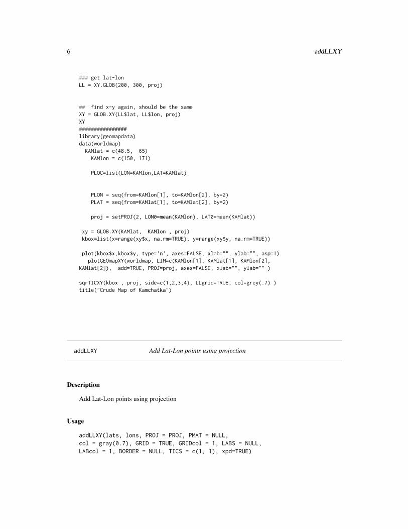
### get lat-lonLL = XY.GLOB(200, 300, proj)

## find x-y again, should be the sameXY = GLOB.XY(LL$lat, LL$lon, proj)XY################library(geomapdata)data(worldmap)

KAMlat = c(48.5, 65)KAMlon = c(150, 171)

PLOC=list(LON=KAMlon,LAT=KAMlat)

PLON = seq(from=KAMlon[1], to=KAMlon[2], by=2)PLAT = seq(from=KAMlat[1], to=KAMlat[2], by=2)

proj = setPROJ(2, LON0=mean(KAMlon), LAT0=mean(KAMlat))

xy = GLOB.XY(KAMlat, KAMlon , proj)kbox=list(x=range(xy$x, na.rm=TRUE), y=range(xy$y, na.rm=TRUE))

plot(kbox$x,kbox$y, type='n', axes=FALSE, xlab="", ylab="", asp=1)plotGEOmapXY(worldmap, LIM=c(KAMlon[1], KAMlat[1], KAMlon[2],

KAMlat[2]), add=TRUE, PROJ=proj, axes=FALSE, xlab="", ylab="" )

sqrTICXY(kbox , proj, side=c(1,2,3,4), LLgrid=TRUE, col=grey(.7) )title("Crude Map of Kamchatka")

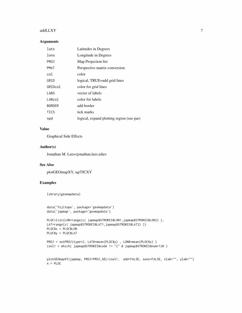
addLLXY Add Lat-Lon points using projection

Description

Add Lat-Lon points using projection

Usage

addLLXY(lats, lons, PROJ = PROJ, PMAT = NULL,col = gray(0.7), GRID = TRUE, GRIDcol = 1, LABS = NULL,LABcol = 1, BORDER = NULL, TICS = c(1, 1), xpd=TRUE)

addLLXY 7

Arguments

lats Latitudes in Degrees

lons Longitude in Degrees

PROJ Map Projection list

PMAT Perspective matrix conversion

col color

GRID logical, TRUE=add grid lines

GRIDcol color for grid lines

LABS vector of labels

LABcol color for labels

BORDER add border

TICS tick marks

xpd logical, expand plotting region (see par)

Value

Graphical Side Effects

Author(s)

Jonathan M. Lees<jonathan.lees.edu>

See Also

plotGEOmapXY, sqrTICXY

Examples

library(geomapdata)

data('fujitopo', package='geomapdata')data('japmap', package='geomapdata')

PLOC=list(LON=range(c( japmap$STROKES$LON1,japmap$STROKES$LON2) ),LAT=range(c( japmap$STROKES$LAT1,japmap$STROKES$LAT2) ))PLOC$x = PLOC$LONPLOC$y = PLOC$LAT

PROJ = setPROJ(type=2, LAT0=mean(PLOC$y) , LON0=mean(PLOC$x) )isel1 = which( japmap$STROKES$code != "i" & japmap$STROKES$num>120 )

plotGEOmapXY(japmap, PROJ=PROJ,SEL=isel1, add=FALSE, axes=FALSE, xlab="", ylab="")A = PLOC

8 addTIX

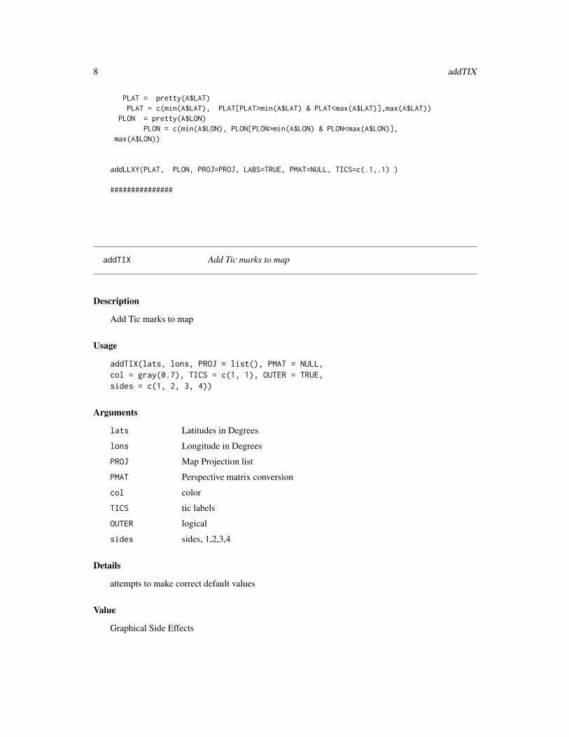
PLAT = pretty(A$LAT)PLAT = c(min(A$LAT), PLAT[PLAT>min(A$LAT) & PLAT<max(A$LAT)],max(A$LAT))

PLON = pretty(A$LON)PLON = c(min(A$LON), PLON[PLON>min(A$LON) & PLON<max(A$LON)],

max(A$LON))

addLLXY(PLAT, PLON, PROJ=PROJ, LABS=TRUE, PMAT=NULL, TICS=c(.1,.1) )

###############

addTIX Add Tic marks to map

Description

Add Tic marks to map

Usage

addTIX(lats, lons, PROJ = list(), PMAT = NULL,col = gray(0.7), TICS = c(1, 1), OUTER = TRUE,sides = c(1, 2, 3, 4))

Arguments

lats Latitudes in Degrees

lons Longitude in Degrees

PROJ Map Projection list


col color

TICS tic labels

OUTER logical

sides sides, 1,2,3,4

Details

attempts to make correct default values

Value


along.great 9

Author(s)


See Also

addLLXY

Examples

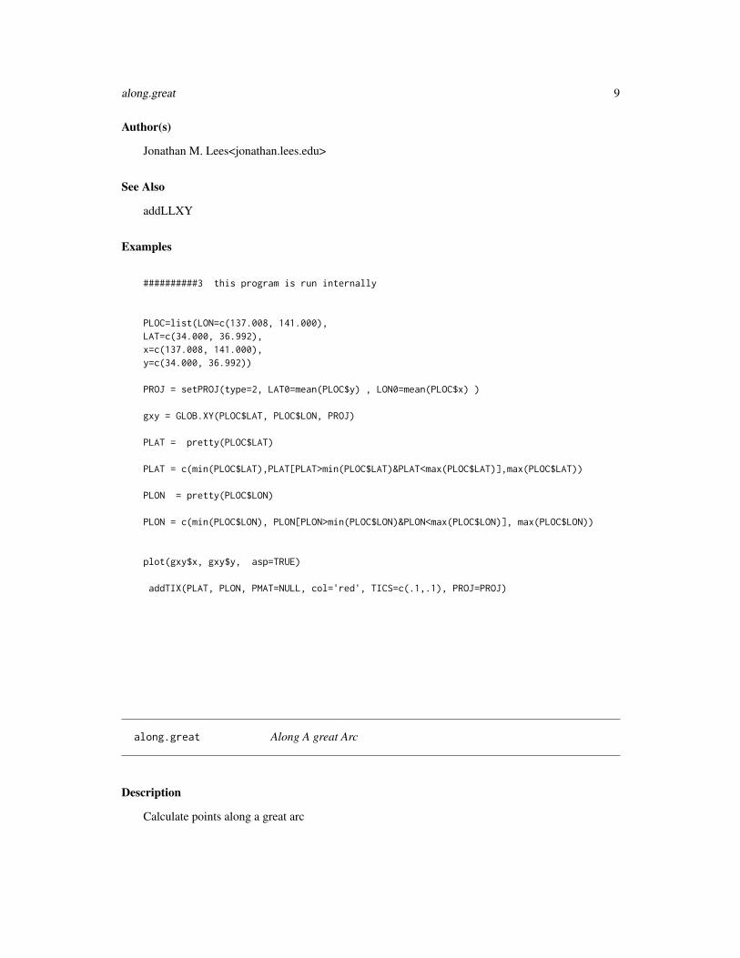
##########3 this program is run internally

PLOC=list(LON=c(137.008, 141.000),LAT=c(34.000, 36.992),x=c(137.008, 141.000),y=c(34.000, 36.992))

PROJ = setPROJ(type=2, LAT0=mean(PLOC$y) , LON0=mean(PLOC$x) )

gxy = GLOB.XY(PLOC$LAT, PLOC$LON, PROJ)

PLAT = pretty(PLOC$LAT)

PLAT = c(min(PLOC$LAT),PLAT[PLAT>min(PLOC$LAT)&PLAT<max(PLOC$LAT)],max(PLOC$LAT))

PLON = pretty(PLOC$LON)

PLON = c(min(PLOC$LON), PLON[PLON>min(PLOC$LON)&PLON<max(PLOC$LON)], max(PLOC$LON))

plot(gxy$x, gxy$y, asp=TRUE)

addTIX(PLAT, PLON, PMAT=NULL, col='red', TICS=c(.1,.1), PROJ=PROJ)

along.great Along A great Arc

Description

Calculate points along a great arc

10 antipolygon

Usage

along.great(phi1, lam0, c, Az)

Arguments

phi1 start lat, radians

lam0 start lon, radians

c distance, radians

Az Azimuthal direction, radiansm

Details

All input and output is radians

Value

List:

phi latitudes, radians

lam longitudes, radians

Author(s)

Jonathan M. Lees<[email protected]>

Examples

lat1 <- 48.856578lon1 <- 2.351828

A = along.great(lat1*pi/180, lon1*pi/180, 50*pi/180, -63*pi/180)

lat=A$phi*180/pilon = A$lam*180/pi

antipolygon Fill the complement of a polygon

Description

Fill a plot with a color outside the confines of a polygon.

Usage

antipolygon(x, y, col = 0, corner=1, pct=.4)

antipolygon 11

Arguments

x x coordinates of polygon

y y coordinates of polygon

col Fill color

corner Corner on the plot to connect to at the end: 1 = LowerLeft(default) ; 2:UpperLeft3 = UpperRight; 4=LowerRight

pct Decimal percent of usr coordinates to expand beyond the polygon

Details

antipolygon uses par("usr") to determine the external bounds of plotting region. Corners are labelsfrom bottom left counter-clockwise, 1-4.

Value

Used for graphical side effect

Note

If the figure is resized after plotting, filling may not appear correct.

Author(s)

Jonathan M. Lees <[email protected]>

See Also

polygon, par

Examples

x = runif(100)y = runif(100)

######### some data points to plot:

plot(x,y)########### create polygon:pp =list(x=c(0.231,0.316,0.169,0.343,0.311,0.484,0.757,

0.555,0.800,0.563,0.427,0.412,0.203),y=c(0.774,0.622,0.401,0.386,0.138,0.312,0.200,0.459,

0.658,0.624,0.954,0.686,0.813))

polygon(pp)

antipolygon(x=pp$x, y=pp$y,col='blue')#### where as this does not look so goodplot(x,y)antipolygon(x=pp$x, y=pp$y,col='blue', corner=2)

12 BASICTOPOMAP

BASICTOPOMAP Basic Topogrpahy Map

Description

Basic Topogrpahy Map

Usage

BASICTOPOMAP(xo, yo, DOIMG, DOCONT, UZ, AZ, IZ, perim, PLAT, PLON,PROJ = PROJ, pnts = NULL, GRIDcol = NULL)

Arguments

xo vector of x-coordinates

yo vector of y-coordinates

DOIMG logical, add image

DOCONT logical, add contours

UZ matrix of image values under sea level

AZ matrix of image values above sea level

IZ matrix of image values

perim perimeter vectors

PLAT latitudes for tic-marks

PLON longitude for tic-marks

PROJ projection list

pnts points to add to plot

GRIDcol color for grid

Details

Image is processed prior to calling

Value

Graphical Side effects

Author(s)


BASICTOPOMAP 13

See Also

DOTOPOMAPI, GEOTOPO

Examples

## Not run:

library(geomapdata)library(MBA) ## for interpolation####### set up topo datadata(fujitopo)##### set up map datadata('japmap', package='geomapdata' )

### target regionPLOC= list(LON=c(138.3152, 139.0214),LAT=c(35.09047, 35.57324))

PLOC$x =PLOC$LONPLOC$y =PLOC$LAT

#### set up projectionPROJ = setPROJ(type=2, LAT0=mean(PLOC$y) , LON0=mean(PLOC$x) )

########## select data from the topo data internal to the targettopotemp = list(lon=fujitopo$lon, lat= fujitopo$lat, z=fujitopo$z)

#### project targetA = GLOB.XY(PLOC$LAT , PLOC$LON , PROJ)

####### select toposelectionflag = topotemp$lat>+PLOC$LAT[1] & topotemp$lat<=PLOC$LAT[2] &topotemp$lon>+PLOC$LON[1] & topotemp$lon<=PLOC$LON[2]

### project topo dataB = GLOB.XY( topotemp$lat[selectionflag] ,topotemp$lon[selectionflag] , PROJ)

### set up out put matrix:### xo = seq(from=range(A$x)[1], to=range(A$x)[2], length=200)### yo = seq(from=range(A$y)[1], to=range(A$y)[2], length=200)

####### interpolation using akima### IZ = interp(x=B$x , y=B$y, z=topotemp$z[selectionflag] , xo=xo, yo=yo)

DF = cbind(x=B$x , y=B$y , z=topotemp$z[selectionflag])IZ = mba.surf(DF, 200, 200, extend=TRUE)$xyz.est

14 bcars

xo = IZ[[1]]yo = IZ[[2]]

### image(IZ)

####### underwater sectionUZ = IZ$zUZ[IZ$z>=0] = NA

#### above sea levelAZ = IZ$zAZ[IZ$z<=-.01] = NA

#### create perimeter:perim= getGEOperim(PLOC$LON, PLOC$LAT, PROJ, 50)

### lats for tic marks:PLAT = pretty(PLOC$LAT)

PLAT = c(min(PLOC$LAT),PLAT[PLAT>min(PLOC$LAT) & PLAT<max(PLOC$LAT)],max(PLOC$LAT))PLON = pretty(PLOC$LON)

### main program:DOIMG = TRUE

DOCONT = TRUEPNTS = NULL

BASICTOPOMAP(xo, yo , DOIMG, DOCONT, UZ, AZ, IZ, perim, PLAT, PLON,PROJ=PROJ, pnts=NULL, GRIDcol=NULL)

### add in the map informationplotGEOmapXY(japmap, LIM=c(PLOC$LON[1], PLOC$LAT[1],PLOC$LON[2],

PLOC$LAT[2]) , PROJ=PROJ, add=TRUE )

## End(Not run)

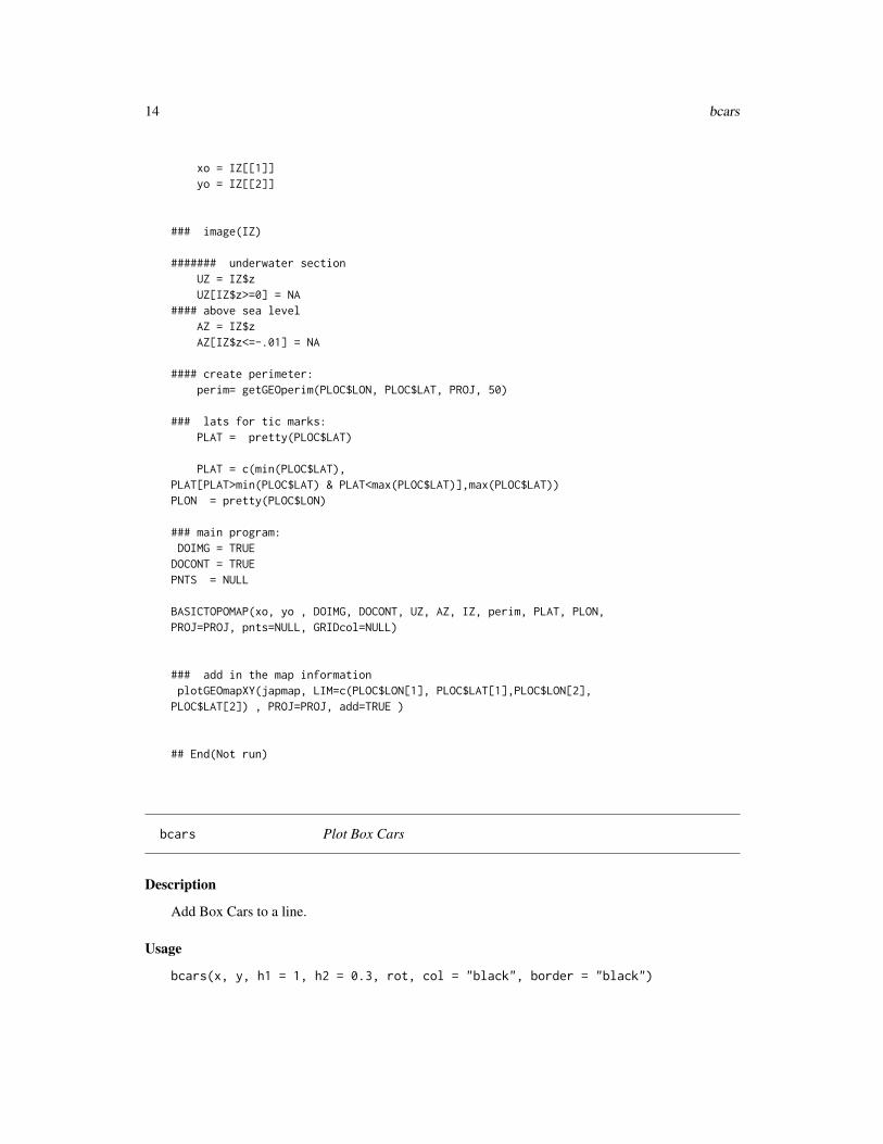
bcars Plot Box Cars

Description

Add Box Cars to a line.

Usage

bcars(x, y, h1 = 1, h2 = 0.3, rot, col = "black", border = "black")

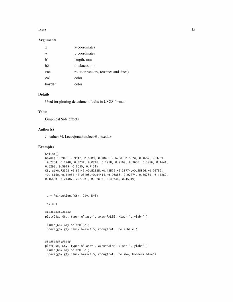
bcars 15

Arguments

x x-coordinates

y y-coordinates

h1 length, mm

h2 thickness, mm

rot rotation vectors, (cosines and sines)

col color

border color

Details

Used for plotting detachment faults in USGS format.

Value


Author(s)


Examples

G=list()G$x=c(-1.0960,-0.9942,-0.8909,-0.7846,-0.6738,-0.5570,-0.4657,-0.3709,-0.2734,-0.1740,-0.0734, 0.0246, 0.1218, 0.2169, 0.3086, 0.3956, 0.4641,0.5293, 0.5919, 0.6530, 0.7131)G$y=c(-0.72392,-0.62145,-0.52135,-0.42599,-0.33774,-0.25896,-0.20759,-0.16160,-0.11981,-0.08105,-0.04414,-0.00885, 0.02774, 0.06759, 0.11262,0.16480, 0.21487, 0.27001, 0.32895, 0.39044, 0.45319)

g = PointsAlong(G$x, G$y, N=6)

sk = 3

###############plot(G$x, G$y, type='n',asp=1, axes=FALSE, xlab='', ylab='')

lines(G$x,G$y,col='blue')bcars(g$x,g$y,h1=sk,h2=sk*.5, rot=g$rot , col='blue')

###############plot(G$x, G$y, type='n',asp=1, axes=FALSE, xlab='', ylab='')lines(G$x,G$y,col='blue')bcars(g$x,g$y,h1=sk,h2=sk*.5, rot=g$rot , col=NA, border='blue')

16 boundGEOmap

boundGEOmap Set Bounds for GEOmap

Description

Given a GEOmap strucutre, set the bounds for the strokes.

Usage

boundGEOmap(MAP, NEGLON = FALSE, projtype = 2)

Arguments

MAP GEOmap structure

NEGLON whether to allow negative longitudes

projtype suggestion (local) map projection to use when getting bounds

Details

Used to rectify a new map after reading in from ascii file. Can take GMT map ascii map files andconvert to GEOmap.

Value

List structure:

STROKES list(nam, num, index, col, style, code, LAT1, LAT2, LON1, LON2)

POINTS list(lat, lon)

PROJ list(type, LAT0, LON0, LAT1, LAT2, LATS, LONS, DLAT, DLON, FE, FN,name)

Author(s)


See Also

worldmap

CCcheck 17

Examples

library(geomapdata)data(worldmap)worldmap = boundGEOmap(worldmap)

CCcheck Counter Clockwise check

Description

Check for counter-clockwise orientation for polygons. Positive is counterclockwise.

Usage

CCcheck(Z)

Arguments

Z list(x,y)

Details

Uses sign of the area of the polygon to determine polarity.

Value

j sign of area

Note

Based on the idea calculated area of a polygon.

Author(s)


Examples

Y=list()Y$x=c(170,175,184,191,194,190,177,166,162,164)Y$y=c(-54,-60,-60,-50,-26,8,34,37,10,-15)

plot(c(160, 200),c(-85, 85), type='n')

18 ccw

points(Y)lines(Y)

CCcheck(Y)

Z = list(x=rev(Y$x), y=rev(Y$y))

CCcheck(Z)

ccw Counter Clockwise Whorl

Description

Used for determining if points are in polygons.

Usage

ccw(p0, p1, p2)

Arguments

p0 point 0

p1 point 1

p2 point 2

Value

returns 1 or 0 depending on position of points

Author(s)


See Also

Lintersect

Examples

l1 = list(p1=list(x=0, y=0), p2=list(x=1,y=1))l2 = list(p1=list(x=6, y=4), p2=list(x=-1,y=-12))

ccw(l1$p1, l1$p2, l2$p1)

coastmap 19

coastmap Global Coast Map

Description

Global Maps of Coast

Usage

data(coastmap)

Format

List structure:



PROJ list(type, LAT0, LON0, LAT1, LAT2, LATS, LONS, DLAT, DLON, FE, FN, name)

Details

This map list is used for filling in coastal lines for global maps. The style=3 is for filling in polygons.The strokes are named for easier access to particular parts ofthe globe. Asia and Africa are onestroke, as are North and South America. there are currently three codes: C=major coast, c=smallercoasts, L=interior lakes.

Examples

data(coastmap)####### see the codes:unique(coastmap$STROKES$code)######### see the different names:unique(coastmap$STROKES$nam)

######### change the colors based on codecoastmap$STROKES$col[coastmap$STROKES$code=="C" ] = rgb(1, .6, .6)coastmap$STROKES$col[coastmap$STROKES$code=="c" ] = rgb(1, .9, .9)coastmap$STROKES$col[coastmap$STROKES$code=="L" ] = rgb(.6, .6, 1)

plotGEOmap(coastmap , border='black' , add=FALSE, xaxs='i')

##

20 ColorScale

ColorScale Color Scale

Description

Graded Color Scale position by locator

Usage

ColorScale(z, loc = list(x = 0, y = 0), thick=1, len=1, offset=.2, col= rainbow(100),border='black', gradcol='black',numbcol='black', unitscol='black',units = "", SIDE = 1, font = 1, fontindex =1, cex=1)

Arguments

z values to be scaled

loc x-y location boundary of plotting area, user coordinates

thick width of scale bar in inches

len length of scale bar in inches

offset offset from border, in inches

col color palette

border color for border of scale, NA=do not plot

gradcol color for gradiation marks of scale, NA=do not plot

numbcol color for number values of scale, NA=do not plot

unitscol color for units character string, NA=do not plot

units character, units for values

SIDE side, 1,2,3,4 as in axis

font vfont number

fontindex font index number

cex character expansion, see par for details

Details

Locations (loc) are given in User coordinates. The scale is plotted relative to the location providedin user coordinates and offset by so many inches outside that unit. to get a scale plotted on theinterior of a plot, send ColorScale a rectangular box inside the plotting region and give it a 0 offset.All other measures are given in inches. To suppress the plotting of a particular item, indicate NAfor its color.

Since the list of the bounding box is returned, this can be used to modify the text, e.g. change theway the units are displayed.

ColorScale 21

Value

list Graphical Side effects and list of bounding box for color scale:

x x coordinates of box

y y coordinates of box

Author(s)


See Also

HOZscale

Examples

data(volcano)

d = dim(volcano)x=seq(from=1,by=1, length=d[1]+1)y=seq(from=1,by=1, length=d[2]+1)plot(range(x), range(y), type='n', asp=1, ann=FALSE, axes=FALSE)

image(x=x, y=y, z=volcano, col = rainbow(100), add=TRUE)

z=volcano

ColorScale(volcano, loc=list(x=range(x), y=range(y)) ,col = rainbow(100), units = "Elev:m", font = 1, SIDE = 1)




plot(range(x), range(y), type='n', asp=1, ann=FALSE, axes=FALSE)

## image(x=x, y=y, z=volcano, col = rainbow(100), add=TRUE)

XAX = pretty(x)XAX = XAX[XAX>=min(x) & XAX<=max(x)]

axis(1, at=XAX, pos=y[1])

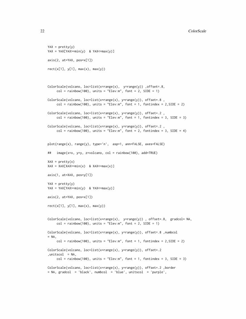
22 ColorScale

YAX = pretty(y)YAX = YAX[YAX>=min(y) & YAX<=max(y)]

axis(2, at=YAX, pos=x[1])

rect(x[1], y[1], max(x), max(y))

ColorScale(volcano, loc=list(x=range(x), y=range(y)) ,offset=.8,col = rainbow(100), units = "Elev:m", font = 2, SIDE = 1)

ColorScale(volcano, loc=list(x=range(x), y=range(y)), offset=.8 ,col = rainbow(100), units = "Elev:m", font = 1, fontindex = 2,SIDE = 2)

ColorScale(volcano, loc=list(x=range(x), y=range(y)), offset=.2 ,col = rainbow(100), units = "Elev:m", font = 1, fontindex = 3, SIDE = 3)

ColorScale(volcano, loc=list(x=range(x), y=range(y)), offset=.2 ,col = rainbow(100), units = "Elev:m", font = 2, fontindex = 3, SIDE = 4)








ColorScale(volcano, loc=list(x=range(x), y=range(y)) , offset=.8, gradcol= NA,col = rainbow(100), units = "Elev:m", font = 2, SIDE = 1)

ColorScale(volcano, loc=list(x=range(x), y=range(y)), offset=.8 ,numbcol= NA,

col = rainbow(100), units = "Elev:m", font = 1, fontindex = 2,SIDE = 2)

ColorScale(volcano, loc=list(x=range(x), y=range(y)), offset=.2,unitscol = NA,

col = rainbow(100), units = "Elev:m", font = 1, fontindex = 3, SIDE = 3)

ColorScale(volcano, loc=list(x=range(x), y=range(y)), offset=.2 ,border= NA, gradcol = 'black', numbcol = 'blue', unitscol = 'purple',

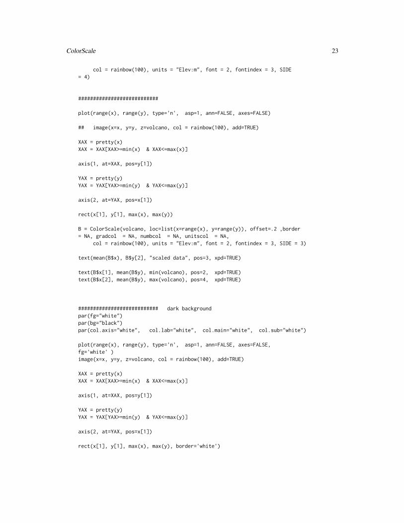
ColorScale 23

col = rainbow(100), units = "Elev:m", font = 2, fontindex = 3, SIDE= 4)

###########################








B = ColorScale(volcano, loc=list(x=range(x), y=range(y)), offset=.2 ,border= NA, gradcol = NA, numbcol = NA, unitscol = NA,


text(mean(B$x), B$y[2], "scaled data", pos=3, xpd=TRUE)

text(B$x[1], mean(B$y), min(volcano), pos=2, xpd=TRUE)text(B$x[2], mean(B$y), max(volcano), pos=4, xpd=TRUE)

########################### dark backgroundpar(fg="white")par(bg="black")par(col.axis="white", col.lab="white", col.main="white", col.sub="white")

plot(range(x), range(y), type='n', asp=1, ann=FALSE, axes=FALSE,fg='white' )image(x=x, y=y, z=volcano, col = rainbow(100), add=TRUE)





rect(x[1], y[1], max(x), max(y), border='white')

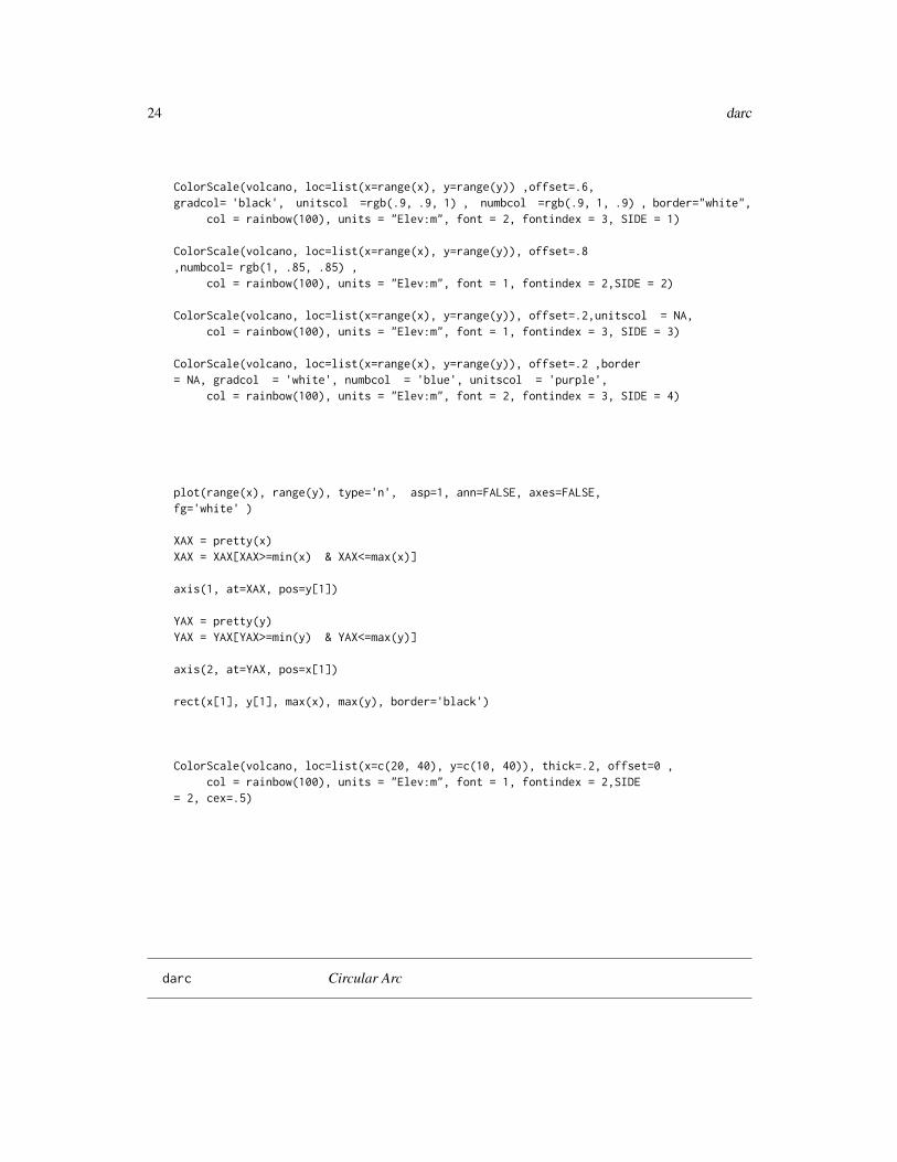
24 darc

ColorScale(volcano, loc=list(x=range(x), y=range(y)) ,offset=.6,gradcol= 'black', unitscol =rgb(.9, .9, 1) , numbcol =rgb(.9, 1, .9) , border="white",


ColorScale(volcano, loc=list(x=range(x), y=range(y)), offset=.8,numbcol= rgb(1, .85, .85) ,

col = rainbow(100), units = "Elev:m", font = 1, fontindex = 2,SIDE = 2)

ColorScale(volcano, loc=list(x=range(x), y=range(y)), offset=.2,unitscol = NA,col = rainbow(100), units = "Elev:m", font = 1, fontindex = 3, SIDE = 3)

ColorScale(volcano, loc=list(x=range(x), y=range(y)), offset=.2 ,border= NA, gradcol = 'white', numbcol = 'blue', unitscol = 'purple',


plot(range(x), range(y), type='n', asp=1, ann=FALSE, axes=FALSE,fg='white' )





rect(x[1], y[1], max(x), max(y), border='black')

ColorScale(volcano, loc=list(x=c(20, 40), y=c(10, 40)), thick=.2, offset=0 ,col = rainbow(100), units = "Elev:m", font = 1, fontindex = 2,SIDE

= 2, cex=.5)

darc Circular Arc

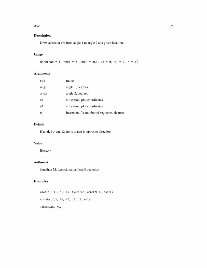
darc 25

Description

Draw acircular arc from angle 1 to angle 2 at a given location.

Usage

darc(rad = 1, ang1 = 0, ang2 = 360, x1 = 0, y1 = 0, n = 1)

Arguments

rad radius

ang1 angle 1, degrees

ang2 angle 2, degrees

x1 x location, plot coordinates

y1 y location, plot coordinates

n increment for number of segments, degrees

Details

If angle1 > angle2 arc is drawn in opposite direction

Value

list(x,y)

Author(s)


Examples

plot(c(0,1), c(0,1), type='n', ann=FALSE, asp=1)

A = darc(.3, 23, 47, .5, .5, n=1)

lines(A$x, A$y)

26 DATUMinfo

DATUMinfo Datum information.

Description

Return a small data base of Datum values for use in UTM projections.

Usage

DATUMinfo()

Details

The function just return a list with the relavent information.

Value

List:

Datum character nameEquatorial Radius, meters (a)

numericPolar Radius, meters (b)

numericFlattening (a-b)/a

numeric

Use character usage

Author(s)


References

websource = http://www.uwgb.edu/dutchs/UsefulData/UTMFormulas.htm

See Also

UTM.xy, UTM.ll, setPROJ

Examples

h = DATUMinfo()data.frame(h)

http://www.uwgb.edu/dutchs/UsefulData/UTMFormulas.htm

demcmap 27

demcmap Color Map from DEM

Description

create a color map from a DEM (Digital Elevation Map)

Usage

demcmap(ZTOPO, n = 100, ccol = NULL)

Arguments

ZTOPO Topography structure

n number of colors

ccol color structure

Value

vector of rgb colors

Author(s)


See Also

rgb, settopocol

difflon Difference between Longitudes

Description

Difference between Longitudes

Usage

difflon(LON1, LON2)

Arguments

LON1 Longitude in degrees

LON2 Longitude in degrees

28 distaz

Details

takes into account crossing the zero longitude

Value

deg degrees difference

sn direction of rotation

Author(s)


Examples

difflon( 34 , 67)

### here we cross the zero linedifflon( 344 , 67)

distaz Distance and Azimuth from two points

Description

Calculate distance, Azimuth and Back-Azimuth from two points on Globe.

Usage

distaz(olat, olon, tlat, tlon)

Arguments

olat origin latitude, degrees

olon origin longitude, degrees

tlat target latitude, degrees

tlon target longitude, degrees

Details

Program is set up for one origin (olat, olon) pair and many target (tlat, tlon) pairs given as vectors.

If multiple olat and olon are given, the program returns a list of outputs for each.

If olat or any tlat is greater than 90 or less than -90 NA is returned and error flag is 0.

If any tlat and tlon is equal to olat and olon, the points are coincident. In that case the distances areset to zero, but the az and baz are NA, and the error flag is set to 0.

distaz 29

Value

List:

del Delta, angle in degreesaz Azimuth, angle in degreesbaz back Azimuth, (az+180) in degreesdist distance in kmerr 0 or 1, error flag. 0=error, 1=no error, see details

Author(s)


See Also

along.great, getgreatarc

Examples

#### one pointd = distaz(12, 23, -32, -65)d

#### many random target pointsorg = c(80.222, -100.940)targ = cbind(runif(10, 10, 50), runif(10, 20, 100))

distaz(org[1], org[2], targ[,1], targ[,2])

############ if origin and target are identical##### the distance is zero, but the az and baz are not defineddistaz(80.222, -100.940, 80.222, -100.940)

######################## set one of the targets equal to the origintarg[7,1] = org[1]targ[7,2] = org[2]


#### put in erroneous latitude data

targ[3,1] = -91.3


30 dms

dms Convert decimal degrees to degree, minutes, seconds

Description

Convert decimal degrees to degree, minutes, seconds

Usage

dms(d1)

Arguments

d1 decomal degrees

Value

list

d degrees

m minutes

s seconds

Author(s)


Examples

dms(33.12345)

H = dms(-91.8765)

print(H)

newH = H$d+H$m/60+H$s/3600print(newH)

DUMPLOC 31

DUMPLOC DUMP vectors to screen in list format

Description

For saving vectors to a file after the locator function has been executed.

Usage

DUMPLOC(zloc, dig = 12)

Arguments

zloc x,y list of locator positions

dig number of digits in output

Value

Side effects: print to screen

Author(s)


Examples

G=list()G$x=c(-1.0960,-0.9942,-0.8909,-0.7846,-0.6738,-0.5570,-0.4657,-0.3709,-0.2734,-0.1740,-0.0734, 0.0246, 0.1218, 0.2169, 0.3086, 0.3956, 0.4641,0.5293, 0.5919, 0.6530, 0.7131)G$y=c(-0.72392,-0.62145,-0.52135,-0.42599,-0.33774,-0.25896,-0.20759,-0.16160,-0.11981,-0.08105,-0.04414,-0.00885, 0.02774, 0.06759, 0.11262,0.16480, 0.21487, 0.27001, 0.32895, 0.39044, 0.45319)

g = PointsAlong(G$x, G$y, N=3)DUMPLOC(g, dig = 5)

32 Ellipsoidal.Distance

EHB.LLZ Earthquake Location Data

Description

Global Earthquake catalog locations from Engdahl, et al.

Usage

data(EHB.LLZ)

Format

lat Latitude

lon Longitude

z depth in km

Source

Data is extrcted from an earthquake data base of relocated events provided by Robert Engdahl.

References

Engdahl, E. R., R. D. van der Hilst, S. H. Kirby, G. Ekstrom, K. M. Shedlock, and A. F. Sheehan(1998), A global survey of slab structures and internal processes using a combined data base ofhigh-resolution earthquake hypocenters, tomographic images and focal mechanism data, Seismol.Res. Lett., 69, 153-154.

Examples

data(EHB.LLZ)## maybe str(EHB.LLZ) ; plot(EHB.LLZ) ...

Ellipsoidal.Distance Ellipsoidal Distance

Description

Ellipsoidal Distance given Latitude and Longitude

Usage

Ellipsoidal.Distance(olat, olon, tlat, tlon, a = 6378137, b = 6356752.314, tol=10^(-12))

Ellipsoidal.Distance 33

Arguments

olat Origin Latitude, degrees

olon Origin Longitude, degrees

tlat Target Latitude, degrees

tlon Target Longitude, degrees

a major axis, meters. If missing uses the

b minor axis, meters

tol Tolerance for convergence, default=10^(-12)

Details

Uses Vincenty’s formulation to calculate the distance along a great circle on an ellipsoidal body.

If a and be are not provided, they are set by default to a=6378137.0 , b=6356752.314, the WGS-84standard.

Only one pair of (olat, olon) and (tlat, tlon) can be given at a time. The program is not vectorized.

Quoting from the wiki page this algorithm was extracted from:

"Vincenty’s formulae are two related iterative methods used in geodesy to calculate the distancebetween two points on the surface of an spheroid, developed by Thaddeus Vincenty in 1975. Theyare based on the assumption that the figure of the Earth is an oblate spheroid, and hence are moreaccurate than methods such as great-circle distance which assume a spherical Earth.

The first (direct) method computes the location of a point which is a given distance and azimuth(direction) from another point. The second (inverse) method computes the geographical distanceand azimuth between two given points. They have been widely used in geodesy because they areaccurate to within 0.5 mm (.020 sec) on the Earth ellipsoid"

Value

list

dist distance, km

az azimuth, degrees

revaz reverse azimuth, degrees

err =0, if convergence failed, else=1

Note

Latitudes >90 and < -90 are not allowed. NA’s are returned.

If points are identical, a distance of zero is returned and NA for the azimuths. If there is someproblems with convergence or division by zero, NA’s are returned and error message is printed.

A couple of known cases that do not work are, e.g.: (olat=0; olon=0; tlat=0; tlon=-180) and (olat=0;olon=0; tlat=0; tlon=180). They will return NA’s to avoid division by zero.

I am not sure how to deal with these cases yet.

The reverse azimuth is the angle from the meridian on the target point to the great circle from theorigin to the target (as far as I can tell). If distaz and Ellipsoidal.Distance are compared, they give

34 Ellipsoidal.Distance

the same azimuth, and the absolute angles of baz (from distaz) and revaz (from Ellipsoidal.Distance)will add to 180 degrees.

Author(s)


References

http://en.wikipedia.org/wiki/Vincenty%27s_formulae

Vincenty, T. (April 1975). Direct and Inverse Solutions of Geodesics on the Ellipsoid with ap-plication of nested equations. Survey Review XXIII (misprinted as XXII) (176): 88.201393.http://www.ngs.noaa.gov/PUBS_LIB/inverse.pdf. Retrieved 2009-07-11.

See Also

distaz

Examples

#### compare to spheroidal calculation distaz####

R.MAPK = 6378.2064N =20

OUT = list(dadist=0, ed2dist=0, ed1dist=0, dif2=0, dif1=0, pct1=0)for( i in 1:N)

{

olat = runif(1, -90, 90)olon = runif(1, 0, 180)

tlat = runif(1, -90, 90)tlon = runif(1, 0, 180)

########## older spherical calculationda = distaz(olat, olon, tlat, tlon)

##### ed1 = elliposidal earthed1 = Ellipsoidal.Distance(olat, olon, tlat, tlon)

##### ed2 spherical earth using############ ellipsoidal calculations, compare withdistaz

ed2 = Ellipsoidal.Distance(olat, olon, tlat, tlon, a=R.MAPK*1000, b=R.MAPK*1000)

dif1 = da$dist-ed1$disdif2 = da$dist-ed2$dis

pct1 = 100*dif1/ed1$dist

Ellipsoidal.Distance 35

############## OUT = format( c(da$dist, ed2$dist, ed1$dist, dif2, dif1, pct1) , digits=10)

OUT$dadist[i] =da$distOUT$ed2dist[i] =ed2$dist

OUT$ed1dist[i]=ed1$distOUT$dif2[i]= dif2OUT$dif1[i]=dif1OUT$pct1[i]=pct1

###cat(paste(collapse=" ", OUT), sep="\n")

}

print( data.frame(OUT) )

############### some extreme cases can cause problems####### here compare Ellipsoidal.Distance with spherical program distaz

Alat = c(90, 90, 90, 90, 45, 45, 45, 45, 0, 0, 0, 0)Alon = c(180, 180,-180, -180, 45, 45, 45, 45, 0, 0, 0, 0)Blat = c(-90, -45, 0, 45, -45, 0, 0, -80, 45, 0, 0, 0)Blon = c(180,-180, 180, 0, -45, 0, -180, 100, -60, -180, 180, 0)

BOUT = list(olat=0, olon=0, tlat=0, tlon=0, dadist=0, ed2dist=0, daaz=0, ed2az=0, dabaz=0, ed2baz=0)

R.MAPK = 6378.2064for(i in 1:length(Alat)){

olat = Alat[i]olon = Alon[i]tlat = Blat[i]tlon = Blon[i]

da = distaz(olat, olon, tlat, tlon)ed2 = Ellipsoidal.Distance(olat, olon, tlat, tlon, a=R.MAPK*1000, b=R.MAPK*1000)cat(paste("i=", i), sep="\n")

BOUT$olon[i] =olonBOUT$olat[i] =olatBOUT$tlat[i] =tlatBOUT$tlon[i] =tlon

BOUT$dadist[i] =da$distBOUT$ed2dist[i] =ed2$dist

BOUT$daaz[i]= da$az

36 eqswath

BOUT$dabaz[i]= da$baz

BOUT$ed2az[i]= ed2$azBOUT$ed2baz[i]= ed2$revaz

}

print(data.frame(BOUT))

eqswath Extract a set of eathquakes in swath along a cross sectional line

Description

Extract a set of eathquakes in swath along a cross sectional line

Usage

eqswath(x, y, z, L, width = 1, PROJ = NULL)

Arguments

x x-coordinates of earthquakes

y y-coordinates of earthquakes

z z-coordinates of earthquakes

L list of x-y coordinates of cross section

width width of swath (km)

PROJ projection information

Details

All units should be the same.

Value

r r-distance along cross section (x-coordinate)

dh distance from cross seection

depth depth in cross section (y-coordinate)

flag index vector of which earthquakes fell in swath and depth range

InvBox coordinates of swath for plotting on map

ExcludeGEOmap 37

Author(s)


See Also

XSECwin, XSECEQ

Examples

############# create datax = runif(100, 1, 100)y = runif(100, 1, 100)z = runif(100, 1, 10)plot(x,y, asp=1)## L = locator()

L=list()L$x=c( 5.42328560757,64.62879777806)L$y=c(89.843266449785,-0.174423911329)

J = eqswath(x, y, z, L, width = 10, PROJ = NULL)

########## show box:plot(x,y, asp=1)lines(J$InvBox$x, J$InvBox$y)

############ show cross section with events plottedplot(J$r, -J$depth)

ExcludeGEOmap Exclude GEOmap Strokes

Description

Select sections of a MAP-list structure based on stroke index

Usage

ExcludeGEOmap(MAP, SEL, INOUT = "out")

Arguments

MAP Map List

SEL Selection of stroke indeces to include or exclude

INOUT text, "in" means include, "out" means exclude

38 expandbound

Value

MAP list

Author(s)


See Also

getGEOmap, plotGEOmap, SELGEOmap, boundGEOmap

Examples

data(coastmap)

### extract (include) the first 6 strokes from world map

A1 = ExcludeGEOmap(coastmap, 1:6, INOUT="in")print(A1$STROKES$nam)

expandbound Expand Bounds

Description

Calculate an expanded bounding region based on a percent of the existing boundaries

Usage

expandbound(g, pct = 0.1)

Arguments

g vector of values

pct fractional percent to expand

Details

uses the range of the exising vector to estimate the expanded bound

Value

vector, new range

explode 39

Author(s)


Examples

i = 5:10exi = expandbound(i, pct = 0.1)range(i)range(exi)

explode Explode Points

Description

Explode a set of points away from a center point

Usage

explode(fxy, dixplo=1, mult=1, cenx=0, ceny=0, PLOT=FALSE)

Arguments

fxy list of x, y coordinates

dixplo distance to explode

mult multiplier for the distance

cenx x coordinate center of explosion

ceny y coordinate center of explosion

PLOT logical, TRUE=make a plot of the resulting explosion

Details

If cenx and ceny is missing it is assumed to be the mean of the coordinates. Program calculates thenew locations radiating away from the central point. No protection against overlapping symbols isincluded.

Value

list of new x,y values

x new x coordinates

y new y coordinates

40 ExplodeSymbols

Author(s)


See Also

ExplodeSymbols, NoOverlap

Examples

############ random datax = rnorm(20)y = rnorm(20)

NEW = explode(list(x=x,y=y), dixplo =1)

plot(range(c(x,NEW$x)), range(c(y,NEW$y)), asp=1, type='n')segments(x,y,NEW$x, NEW$y)points(x,y, pch=3, col='red')points(NEW$x, NEW$y, pch=6, col='blue', cex=2)

### try a larger radius:NEW2 = explode(list(x=x,y=y), dixplo =1.3)points(NEW2$x, NEW2$y, pch=7, col='brown', cex=2, xpd=TRUE)arrows(NEW$x, NEW$y,NEW2$x, NEW2$y, col='green' )

##### try with a different centercenx=-1; ceny=-1NEW = explode(list(x=x,y=y), dixplo =1, cenx=cenx, ceny=ceny)plot(range(c(x,NEW$x)), range(c(y,NEW$y)), asp=1, type='n')points(x,y, pch=3, col='red')segments(x,y,NEW$x, NEW$y)points(NEW$x, NEW$y, pch=6, col='blue', cex=2)points(cenx, ceny, pch=8, col='purple')text(cenx, ceny, labels="Center Point", pos=1)

ExplodeSymbols Explode symbols that overlap

Description

Interactive program for redistributing symbols for later plotting. Used for Focal Mechanisms.

ExplodeSymbols 41

Usage

ExplodeSymbols(XY, fsiz = 1, STARTXY = NULL, MAP = NULL)

Arguments

XY list of x,y values

fsiz size of the symbol, as a percentage of the user coordinates

STARTXY Starting positions. This is used for multiple sessions where we want to pick upthe previous locations.

MAP Map to plot on the screen, in GEOmap format.

Details

The program is interactive. It starts by plotting the points as symbols. A number of buttons areprovided for exploding the points semi automatically. To move each point click near its currentpoint, then click at the destination followed by a click on the HAND button. several symbols canbe moved at the same time.

You must click on the screen and on the buttons to get this code working - the program will notwork in batch mode or run as a script You click in the active screen area and then press a button ontop (or bottom) - the button takes your clicks and does something Here are some hints:

Buttons:Buttons appear on top and bottom of the plotting region.

HAND: If you want to move only one symbol (focal mech) click near it and then click where youwant it to go. Then click the HAND button You may click several at once, but for each click oin asymbol there has to be a click somewhere to relocate it. (i.e. there must be an even number of clickson the screen before hitting the HAND button)

SEL: If you want to explode several symbols at once, first select them: click lower left, then upperright of rectangle enclosing the selection. Once a selection is made it remains active until anotherselection is made so you can keep changing the radius and center for different explosions Then clickCIRC.

RECT Choose a rectangle (lower left and upper right), then click RECT for an explosion

RECT2 After selecting, choose a center and a distance. symbols will be moved to a rectangularperimeter defined by the two points

CIRC After selection, click once for the circle center, and a second time for the radius, then clickCIRC

LINE After selection,will explode the events away from a line, a given distance away. The line isgiven by 2 points and the distance by a third perpendicular distance.

Value

list of new x,y values

Note

For now the map is given in lat-lon coordinates- the same as the points being moved. There is nomap projection used.

42 faultdip

Author(s)


See Also

rekt2line

Examples

## Not run:F1 = list(x=rnorm(43), y=rnorm(43))SMXY = ExplodeSymbols(F1, 0.03)

## End(Not run)

faultdip Show Fault dip

Description

Show Fault dip

Usage

faultdip(x, y, rot = 0, h = 1, lab = "")

Arguments

x x-coordinates

y y-coordinates

rot cosine and sine of rotation

h length of mark

lab labels

Value

Graphical Side effect

Author(s)


faultperp 43

See Also

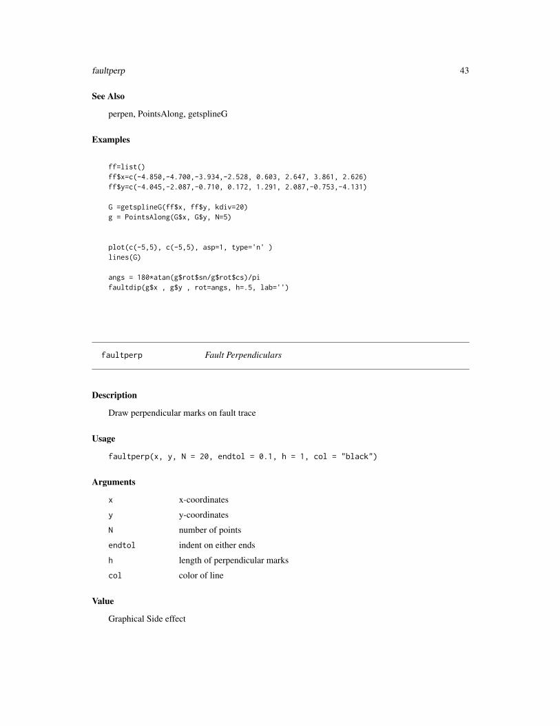
perpen, PointsAlong, getsplineG

Examples

ff=list()ff$x=c(-4.850,-4.700,-3.934,-2.528, 0.603, 2.647, 3.861, 2.626)ff$y=c(-4.045,-2.087,-0.710, 0.172, 1.291, 2.087,-0.753,-4.131)

G =getsplineG(ff$x, ff$y, kdiv=20)g = PointsAlong(G$x, G$y, N=5)

plot(c(-5,5), c(-5,5), asp=1, type='n' )lines(G)

angs = 180*atan(g$rot$sn/g$rot$cs)/pifaultdip(g$x , g$y , rot=angs, h=.5, lab='')

faultperp Fault Perpendiculars

Description

Draw perpendicular marks on fault trace

Usage

faultperp(x, y, N = 20, endtol = 0.1, h = 1, col = "black")

Arguments

x x-coordinates

y y-coordinates

N number of points

endtol indent on either ends

h length of perpendicular marks

col color of line

Value


44 fixCoastwrap

Author(s)


See Also

OverTurned

Examples

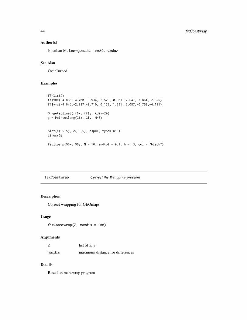
ff=list()ff$x=c(-4.850,-4.700,-3.934,-2.528, 0.603, 2.647, 3.861, 2.626)ff$y=c(-4.045,-2.087,-0.710, 0.172, 1.291, 2.087,-0.753,-4.131)



faultperp(G$x, G$y, N = 10, endtol = 0.1, h = .3, col = "black")

fixCoastwrap Correct the Wrapping problem

Description

Correct wrapping for GEOmaps

Usage

fixCoastwrap(Z, maxdis = 100)

Arguments

Z list of x, y

maxdis maximum distance for differences

Details

Based on mapswrap program

gclc 45

Value

List:

x x-coordinates (longitudes)

y y-coordinates (latitudes)

Author(s)


Examples

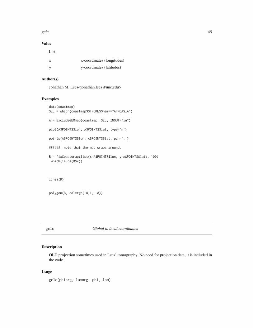
data(coastmap)SEL = which(coastmap$STROKES$nam=="AFROASIA")

A = ExcludeGEOmap(coastmap, SEL, INOUT="in")

plot(A$POINTS$lon, A$POINTS$lat, type='n')

points(A$POINTS$lon, A$POINTS$lat, pch='.')

###### note that the map wraps around.

B = fixCoastwrap(list(x=A$POINTS$lon, y=A$POINTS$lat), 100)which(is.na(B$x))

lines(B)

polygon(B, col=rgb(.8,1, .8))

gclc Global to local coordinates

Description

OLD projection sometimes used in Lees’ tomography. No need for projection data, it is included inthe code.

Usage

gclc(phiorg, lamorg, phi, lam)

46 geoarea

Arguments

phiorg lat origin

lamorg lon origin

phi lat

lam lon

Details

This may be defunct now.

Value

x coordinate, km

y coordinate, km

Note

Orignally from R. S. Crosson

Author(s)


See Also

lcgc

Examples

gclc(23, 35, 23.5, 35.6)

geoarea Area of Map objects

Description

vector of areas of polygons in map

Usage

geoarea(MAP, proj=NULL, ncut=10)

Arguments

MAP Map structure

proj projection

ncut minimum number of points in polygon

geoLEGEND 47

Details

Uses splancs function. If proj is NULL then the project is reset to UTM spherical for each elementseperately to calculate the area in km. ncut is used to eliminate area calculations with strokes lessthan the specified number.

Value

vector of areas

Note

areas smaller than a certain tolerance are NA

Author(s)


geoLEGEND Geological legend from GEOmap Structure

Description

Create and add Geological legend from GEOmap Structure

Usage

geoLEGEND(names, shades, zx, zy, nx, ny, side=1, cex=0.5)

Arguments

names namesof units

shades colorsof units

zx width of box, mm

zy height of box, mm

nx number of boxes in x-direction

ny number of boxes in y-direction

side Side of the plot for the legend (1,2,3,4)

cex Character expansion for text in legend

Details

Adds geological legend based on information provided. Legend is placed in margin.

Value


48 geoLEGEND

Note

If plot is resized, should re-run this as the units depend on the screen size information and thetransformation of user coordinates.

Author(s)


Examples

## Not run:

library(RPMG)library(RSEIS)library(GEOmap)library(geomapdata)

data(cosogeol)data(cosomap)

data(faults)data(hiways)data(owens)

proj = cosomap$PROJ

XMCOL = setXMCOL()

newcol = XMCOL[cosogeol$STROKES$col+1]cosocolnums = cosogeol$STROKES$colcosogeol$STROKES$col = newcolss = strsplit(cosogeol$STROKES$nam, split="_")

geo = unlist(sapply(ss , "[[", 1))

UGEO = unique(geo)

mgeo = match( geo, UGEO )

gcol = paste(sep=".", geo, cosogeol$STROKES$col)

ucol = unique(gcol)

N = length(ucol)

spucol = strsplit(ucol,split="\.")

geoLEGEND 49

names = unlist(sapply(spucol , "[[", 1))

shades = unlist(sapply(spucol , "[[", 2))

ORDN = order(names)### example:

par(mai=c(0.5, 1.5, 0.5, 0.5) )

plotGEOmapXY(cosomap, PROJ=proj, add=FALSE, ann=FALSE, axes=FALSE)

plotGEOmapXY(cosogeol, PROJ=proj, add=TRUE, ann=FALSE, axes=FALSE)

geoLEGEND(names[ORDN], shades[ORDN], .28, .14, 4, 16, side=2)

####par(mai=c(0.5, 0.5, 1.0, 0.5) )




####par(mai=c(0.5, 0.5, 0.5, 1) )




####par(mai=c(1.5, 0.5, 0.5, 0.5) )




## End(Not run)

50 GEOmap.breakpoly

GEOmap.breakline Break a line at specified indeces into a list

Description

Break a line at specified indices into a list

Usage

GEOmap.breakline(Z, ww)

Arguments

Z list of x,y location values

ww index vector of break locations

Value

newx list x of strokes

newy list y of strokes

Author(s)


Examples

Y=list()Y$x=c(170,175,184,191,194,190,177,166,162,164)Y$y=c(-54,-60,-60,-50,-26,8,34,37,10,-15)

GEOmap.breakline(Y, 5)

GEOmap.breakpoly Break up a polygon

Description

Break up a polygon

Usage

GEOmap.breakpoly(Z, ww)

GEOmap.cat 51

Arguments

Z list, x,y locations

ww vector of indecies where NAs occur

Details

The NA values in Z represent breaks. GEOmap.breakpoly breaks the polygon up into individualstrokes. The beginning and the ending of the stroke are combined.

Value

newx list of x values

newy list of y values

Author(s)


See Also

fixCoastwrap, GEOmap.breakline

Examples

x=1:100y = 1:100

ww = c(25, 53, 75)

A = list(x=x, y=y)

W = GEOmap.breakpoly(A , ww)

GEOmap.cat Concatenate Two GEOmaps

Description

Combine Two GEOmaps into one

Usage

GEOmap.cat(MAP1, MAP2)

52 GEOmap.CombineStrokes

Arguments

MAP1 GEOmap list

MAP2 GEOmap list

Details

Maps are combine consecutively.

Value

GEOmap list

Author(s)


See Also

GEOmap.Extract, GEOmap.CombineStrokes, list.GEOmap

Examples

data(coastmap)CUBA = GEOmap.Extract(coastmap,90, INOUT="in" )

NSAMER = GEOmap.Extract(coastmap,2, INOUT="in" )AMAP = GEOmap.cat(CUBA, NSAMER)plotGEOmap(AMAP )

GEOmap.CombineStrokes Combine strokes in a GEOmap list

Description

Combine strokes in a GEOmap list

Usage

GEOmap.CombineStrokes(MAP, SEL)

Arguments

MAP GEOmap list

SEL index of strokes to be combined

GEOmap.Extract 53

Details

Stokes are combined in the order designated by the SEL index vector. The direction of the strokesis not modified - this may have to be fixed so that strokes align properly.

Value

GEOmap list

STROKES Metadata for strokes

POINTS list, lat=vector, lon=vector

Author(s)


See Also

GEOmap.cat, GEOmap.Extract, GEOmap.CombineStrokes, list.GEOmap

Examples

data(coastmap)SEL = which(coastmap$STROKES$nam=="Caribbean")

CAR = GEOmap.Extract(coastmap, SEL, INOUT="in" )

plotGEOmap(CAR, MAPstyle=3, NUMB=TRUE)

CAR2 = GEOmap.CombineStrokes(CAR, SEL =c(6:15) )

plotGEOmap(CAR2, MAPstyle=3, MAPcol='red' , add=TRUE)

GEOmap.Extract Extract from GEOmap

Description

Extract or Exclude parts of a GEOmap list.

Usage

GEOmap.Extract(MAP, SEL, INOUT = "out")fastExtract(MAP, SEL, INOUT = "out")GEOmap.limit(MAP, LLlim )

54 GEOmap.list

Arguments

MAP GEOmap List

SEL Selection of stroke indeces to include or exclude

INOUT text, "in" means include, "out" means exclude

LLlim vector latlon limits

Details

Can either extract from the GEOmap data list with in, or exclude with out. fastExtract is the samebut may be faster since it does not process all the strokes in the base GEOmap.

Value

GEOmap list

Author(s)


See Also

GEOmap.cat, GEOmap.Extract, GEOmap.CombineStrokes, list.GEOmap, getGEOmap, plotGE-Omap, SELGEOmap, boundGEOmap,

Examples

data(coastmap)SEL=which(coastmap$STROKES$nam=="AMERICAS")NSAMER = GEOmap.Extract(coastmap,SEL, INOUT="in" )plotGEOmap(NSAMER)

GEOmap.list GEOmap to list

Description

Inverse of list.GEOmap.

Usage

GEOmap.list(MAP, SEL = 1)

Arguments

MAP GEOmap list

SEL index, selecttion of specific strokes

GEOsymbols 55

Details

Returns the GEOmap strokes and instead of a long vector for the points they are broken down intoa list of strokes.

Value



LL list of lat-lon strokes

Author(s)


See Also

GEOmap.cat, GEOmap.Extract, GEOmap.CombineStrokes, list.GEOmap

Examples

data(coastmap)SEL=which(coastmap$STROKES$nam=='CUBA')G = GEOmap.list(coastmap, SEL=SEL )

### Lat-Lon of CubaG$LL

GEOsymbols GEOsymbols

Description

Plot a set of Geological Symbols

Usage

GEOsymbols()

Details

Currently the choices in symbols are:contact anticline syncline OverTurned-ant OverTurned-syn perp thrust normal dextral sinestraldetachment bcars

56 GEOTOPO

Value


Author(s)


See Also

bcars, thrust, teeth, SynAnticline, SSfault, horseshoe, strikeslip, OverTurned, normalfault, PointsA-long

Examples

GEOsymbols()

GEOTOPO Topographic Plot of geographic region

Description

Extract subset of a topographic database, interpolate and plot using the persp program.

Usage

GEOTOPO(TOPO, PLOC, PROJ, calcol=NULL, nx=500, ny=500, nb = 4, mb = 4, hb = 8, PLOT=TRUE)

Arguments

TOPO list of x,y,z for a DEM

PLOC Location list, includes vectors LON and Lat

PROJ projection

calcol color table for coloring elevations above sea level

nx number of points in x grid, default=500

ny number of points in y grid, default=500

nb see function mba.surf, default = 4

mb see function mba.surf, default = 4

hb see function mba.surf , default= 8

PLOT logical, TRUE=plot a map and return color map

GEOTOPO 57

Details

The return matrix PMAT is a rotation matrix used for adding geographic (projected) data onto theperspective plot.

Value

PMAT Matrix from persp, used for adding other geographic information

xo x-coordinates

yo y-coordinates

IZ interpolated elevations

Cmat matrix of RGB Colors

Dcol dimensions of Cmat

Note

If PLOT is false the transform matrix PMAT and the color mapping matrix Cmat will be returnedas NA. To create these for future plotting, use TOPOCOL or LandSeaCol functions. TOPOCOLsimply assigns values above sea level with one color scale and those below with under water colors.LandSeaCol requires a coastal map and fills in land areas with terrain colors and sea areas with bluepalette colors.

Author(s)


See Also

subsetTOPO, TOPOCOL, LandSeaCol, settopocol, subsetTOPO, persp, DOTOPOMAPI

Examples

## Not run:

library(geomapdata)

data(ETOPO5)PLOC=list(LON=c(137.008, 141.000),LAT=c(34.000, 36.992),

x=c(137.008, 141.000), y=c(34.000, 36.992) )

PROJ = setPROJ(type=2, LAT0=mean(PLOC$y) , LON0=mean(PLOC$x) )COLS = settopocol()JMAT = GEOTOPO(ETOPO5, PLOC, PROJ, COLS$calcol, nx=1000, ny=1000, nb=8, mb=8, hb=12, PLOT=TRUE)

############ this plot can be duplicated by using the output or GEOTOPO

58 getETOPO

PMAT = persp(JMAT$xo, JMAT$yo, JMAT$IZ$z, theta = 0, phi = 90, r=4000,col=JMAT$Cmat[1:(JMAT$Dcol[1]-1), 1:(JMAT$Dcol[2]-1)] , scale = FALSE,

ltheta = 120, lphi=60, shade = 0.75, border = NA, expand=0.001, box = FALSE )

## End(Not run)

getETOPO Get Subset ETOPO Digital elevation map

Description

Extract from ETOPO5 or ETOPO2 data a rectangular subset of the full data.

Usage

getETOPO(topo, glat = c(-90, 90), glon = c(0, 360))

Arguments

topo A DEM matrix, ETOPO5 or ETOPO2

glat 2-vector, latitude limits

glon 2-vector, longitude limits (these are converted 0-360

Details

ETOPO2 and ETOPO5 are stored in a strange way: the lons are okay the latitudes are upside down.

Value

returns a matrix with attributes in lat-lon that are correct for usage in image or other R imagingprograms.

Author(s)


See Also

image

getGEOmap 59

Examples

library(geomapdata)

data(ETOPO5)

glat =c(45.4, 49)glon = c(235, 243)b5 = getETOPO(ETOPO5, glat, glon)image(x=attr(b5, 'lon'), y=attr(b5,'lat'), z=b5, col=terrain.colors(100) )contour( x=attr(b5, 'lon'), y=attr(b5,'lat'), z=b5, add=TRUE)

getGEOmap Get Geomap

Description

Get Geomap from ascii files

Usage

getGEOmap(fn)

Arguments

fn root name

Details

Files are stored as a pair: rootname.strks and rootname.pnts

Value

STROKES List of stroke information:nam name of strokenum number of pointsindex index where points startcol colorstyle plotting style: 1=point, 2=line,3=polygoncode character, geological codeLAT1 bounding box lower left LatLAT2 bounding box upper right LatLON1 bounding box lower left LonLON2 bounding box upper right LonPOINTS List of point LL coordinates, list(lat, lon)PROJ optional projection parameters

60 getGEOperim

Author(s)


See Also

plotGEOmapXY, boundGEOmap

Examples

## Not run:library(geomapdata)

data(cosomap)data(faults)data(hiways)data(owens)

cosogeol = getGEOmap("/home/lees/XMdemo/GEOTHERM/cosogeol")

cosogeol = boundGEOmap(cosogeol)

proj = cosomap$PROJ



plotGEOmapXY(cosomap, PROJ=proj, add=TRUE, ann=FALSE, axes=FALSE)

plotGEOmapXY(faults, PROJ=proj, add=TRUE, ann=FALSE, axes=FALSE)

## End(Not run)

getGEOperim Get Lat-Lon Perimeter

Description

Get rectangular perimeter of region defined by set of Lat-Lon

Usage

getGEOperim(lon, lat, PROJ, N)

getgreatarc 61

Arguments

lon vector of lons

lat vector of lats

PROJ projection structure

N number of points per side

Details

perimeter is used for antipolygon

Value

List:

x x-coordinates projected

y y-coordinates projected

Author(s)


Examples

### target regionPLOC= list(LON=c(138.3152, 139.0214),LAT=c(35.09047, 35.57324))

PLOC$x =PLOC$LONPLOC$y =PLOC$LAT

#### set up projectionPROJ = setPROJ(type=2, LAT0=mean(PLOC$y) , LON0=mean(PLOC$x) )

perim= getGEOperim(PLOC$LON, PLOC$LAT, PROJ, 50)

getgreatarc Great Circle Arc

Description

Get points along great circle between two locations

62 getgreatarc

Usage

getgreatarc(lat1, lon1, lat2, lon2, num)

Arguments

lat1 Latitude, point 1 (degrees)

lon1 Longitude, point 1 (degrees)

lat2 Latitude, point 2 (degrees)

lon2 Longitude, point 2 (degrees)

num number of points along arc

Value

lat Latitude

lon Longitude

Author(s)


See Also

getgreatarc, distaz

Examples

PARIS = c(48.8666666666667, 2.33333333333333)RIODEJANEIRO =c( -22.9, -43.2333333333333)

g = getgreatarc(PARIS[1],PARIS[2], RIODEJANEIRO[1], RIODEJANEIRO[2],100)library(geomapdata)data(worldmap)

plotGEOmap(worldmap, add=FALSE, shiftlon=180)

lines(g$lon+180, g$lat)

getmagsize 63

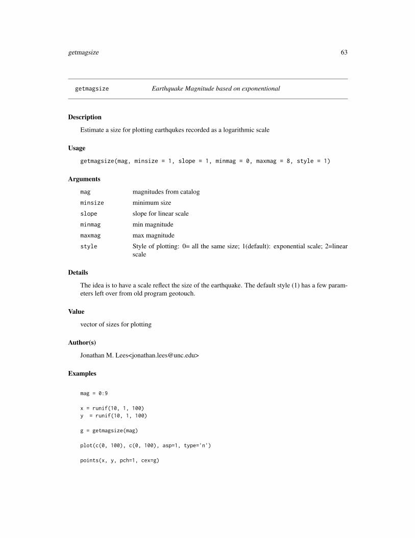
getmagsize Earthquake Magnitude based on exponentional

Description

Estimate a size for plotting earthqukes recorded as a logarithmic scale

Usage

getmagsize(mag, minsize = 1, slope = 1, minmag = 0, maxmag = 8, style = 1)

Arguments

mag magnitudes from catalog

minsize minimum size

slope slope for linear scale

minmag min magnitude

maxmag max magnitude

style Style of plotting: 0= all the same size; 1(default): exponential scale; 2=linearscale

Details

The idea is to have a scale reflect the size of the earthquake. The default style (1) has a few param-eters left over from old program geotouch.

Value

vector of sizes for plotting

Author(s)


Examples

mag = 0:9

x = runif(10, 1, 100)y = runif(10, 1, 100)

g = getmagsize(mag)

plot(c(0, 100), c(0, 100), asp=1, type='n')

points(x, y, pch=1, cex=g)

64 getnicetix

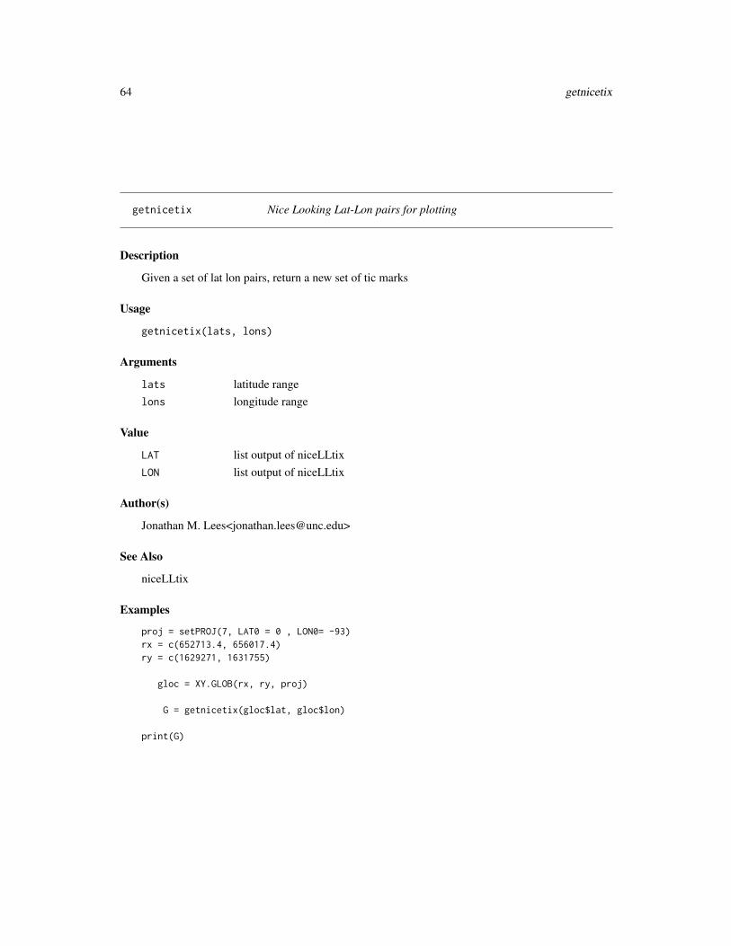
getnicetix Nice Looking Lat-Lon pairs for plotting

Description

Given a set of lat lon pairs, return a new set of tic marks

Usage

getnicetix(lats, lons)

Arguments

lats latitude rangelons longitude range

Value

LAT list output of niceLLtixLON list output of niceLLtix

Author(s)


See Also

niceLLtix

Examples

proj = setPROJ(7, LAT0 = 0 , LON0= -93)rx = c(652713.4, 656017.4)ry = c(1629271, 1631755)

gloc = XY.GLOB(rx, ry, proj)

G = getnicetix(gloc$lat, gloc$lon)

print(G)

getspline 65

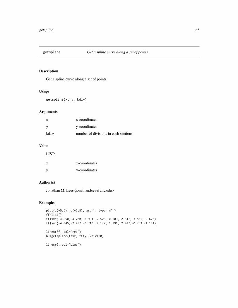
getspline Get a spline curve along a set of points

Description

Get a spline curve along a set of points

Usage

getspline(x, y, kdiv)

Arguments

x x-coordinates

y y-coordinates

kdiv number of divisions in each sections

Value

LIST:

x x-coordinates

y y-coordinates

Author(s)


Examples

plot(c(-5,5), c(-5,5), asp=1, type='n' )ff=list()ff$x=c(-4.850,-4.700,-3.934,-2.528, 0.603, 2.647, 3.861, 2.626)ff$y=c(-4.045,-2.087,-0.710, 0.172, 1.291, 2.087,-0.753,-4.131)

lines(ff, col='red')G =getspline(ff$x, ff$y, kdiv=20)

lines(G, col='blue')

66 getsplineG

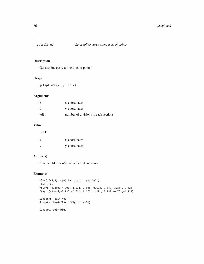
getsplineG Get a spline curve along a set of points

Description

Get a spline curve along a set of points

Usage

getsplineG(x, y, kdiv)

Arguments

x x-coordinates

y y-coordinates

kdiv number of divisions in each sections

Value

LIST:

x x-coordinates

y y-coordinates

Author(s)


Examples


lines(ff, col='red')G =getsplineG(ff$x, ff$y, kdiv=20)

lines(G, col='blue')

GETXprofile 67

GETXprofile Cross sectional profile through a digital elevation map

Description

Example of how to use RPMG button functions. This example shows how to plot a DEM andinteractively change the plot and find projected cross-sections through a surface.

Usage

GETXprofile(jx, jy, jz, LAB = "A", myloc = NULL, PLOT = FALSE, NEWDEV=TRUE, asp=1)

Arguments

jx, jy locations of grid lines at which the values in ’jz’ are measured.

jz a matrix containing the values to be plotted

LAB Alphanumeric (A-Z) for labeling a cross section

myloc Out put of Locator function

PLOT logical. Plot is created if TRUE

NEWDEV logical. Plot is on a new device if TRUE

asp aspect ration for plotting, see par

Details

The program uses a similar input format as image or contour, with structure from the locator()function of x and y coordinates that determine where the cross section is to be extracted.

Value

Returns a list of x,z values representing the projected values along the cross section.

RX distance along cross section

RZ values extracted from the elevation map

Note

The program is an auxiliary program provided to illustrate the RPMG interactive R analysis.

Author(s)


See Also

locator, image

68 GLOB.XY

Examples

## Not run:####### get data

data(volcano)#### extract dimensions of image

nx = dim(volcano)[1]ny = dim(volcano)[2]

### establish units of imagejx = 10*seq(from=0, to=nx-1)jy = 10*seq(from=0, to=ny-1)

#### set a letter for the cross sectionLAB = LETTERS[1]

### coordinates of cross section on image### this is normally set by using the locator() function

x1 = 76.47351y1 = 231.89055x2 = 739.99746y2 = 464.08185

## extract and plot cross section

GETXprofile(jx, jy, volcano, myloc=list(x=c(x1, x2), y=c(y1, y2)), LAB=LAB, PLOT=TRUE)

## End(Not run)

GLOB.XY Convert from GLOBAL LAT-LON to X-Y

Description

Convert from GLOBAL LAT-LON to X-Y

Usage

GLOB.XY(LAT, LON, PROJ.DATA)

Arguments

LAT Latitude

LON Longitude

PROJ.DATA Projection list

Details

Units should be given according to the projection. This is the inverse of XY.GLOB.

GLOBE.ORTH 69

Value

x X in whatever units

y Y in whatever units

Author(s)


References


See Also

XY.GLOB

Examples

proj = setPROJ(type = 2, LAT0 =23, LON0 = 35)

### get lat-lonLL = XY.GLOB(200, 300, proj)

## find x-y again, should be the sameXY = GLOB.XY(LL$lat, LL$lon, proj)XY

GLOBE.ORTH Plot globe with orthogonal

Description

Plot globe with orthogonal

Usage

GLOBE.ORTH(lam0, phi1, R = 1, plotmap = TRUE, plotline=TRUE, add=FALSE,map = coastmap, mapcol = grey(0.2), linecol = grey(0.7), fill=FALSE)

70 GLOBE.ORTH

Arguments

lam0 view origin longitude, degrees

phi1 view origin latitude, degrees

R Radius of sphere, default=1

plotmap logical, default=TRUE, add map

plotline logical, default=TRUE, add grid of lat-lons

add logical, default=FALSE, Do not start a new plot, rather add to existing plot

map GEOmap list

mapcol color for map

linecol color for meridians and parallels

fill fill polygons with color, default=FALSE

Details

Plots whole globe with grid.

Value


Author(s)


References


See Also

setPROJ, projtype, plotGEOmap

Examples

###### simple map of world viewed at 40 degrees latitudeR = 1R.MAPK = 6378.2064

phi1=40

viewlam = seq(from=0, to=340, by=2)

data(coastmap)

K=1GLOBE.ORTH(viewlam[K], phi1, R=1, plotmap=TRUE)######

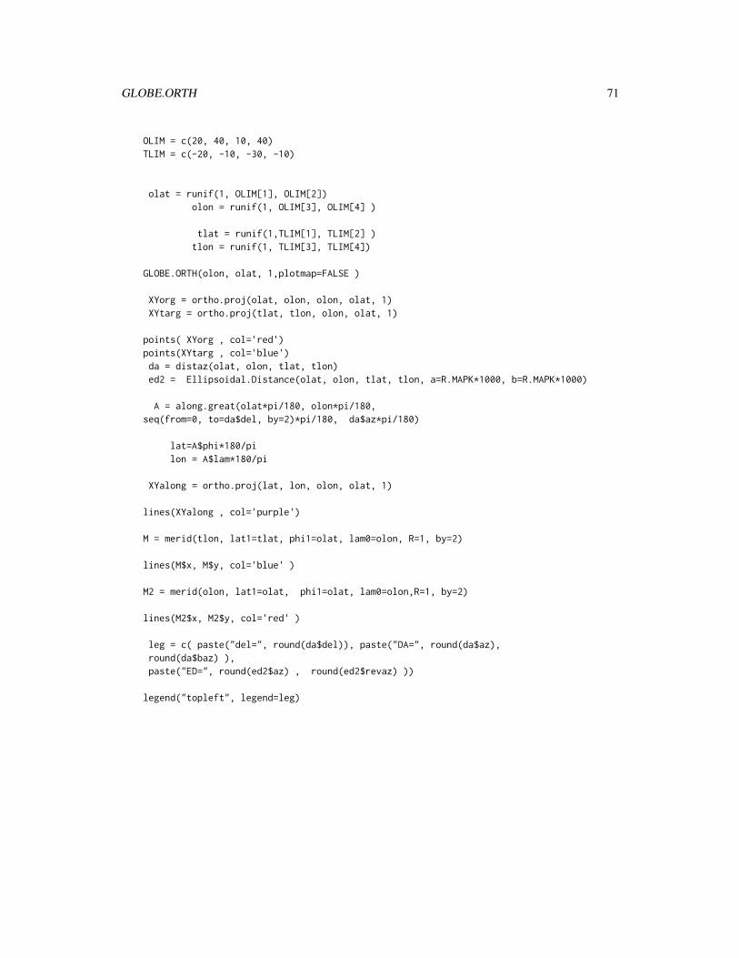
GLOBE.ORTH 71

OLIM = c(20, 40, 10, 40)TLIM = c(-20, -10, -30, -10)

olat = runif(1, OLIM[1], OLIM[2])olon = runif(1, OLIM[3], OLIM[4] )

tlat = runif(1,TLIM[1], TLIM[2] )tlon = runif(1, TLIM[3], TLIM[4])

GLOBE.ORTH(olon, olat, 1,plotmap=FALSE )

XYorg = ortho.proj(olat, olon, olon, olat, 1)XYtarg = ortho.proj(tlat, tlon, olon, olat, 1)

points( XYorg , col='red')points(XYtarg , col='blue')da = distaz(olat, olon, tlat, tlon)ed2 = Ellipsoidal.Distance(olat, olon, tlat, tlon, a=R.MAPK*1000, b=R.MAPK*1000)

A = along.great(olat*pi/180, olon*pi/180,seq(from=0, to=da$del, by=2)*pi/180, da$az*pi/180)

lat=A$phi*180/pilon = A$lam*180/pi

XYalong = ortho.proj(lat, lon, olon, olat, 1)

lines(XYalong , col='purple')

M = merid(tlon, lat1=tlat, phi1=olat, lam0=olon, R=1, by=2)

lines(M$x, M$y, col='blue' )

M2 = merid(olon, lat1=olat, phi1=olat, lam0=olon,R=1, by=2)

lines(M2$x, M2$y, col='red' )

leg = c( paste("del=", round(da$del)), paste("DA=", round(da$az),round(da$baz) ),paste("ED=", round(ed2$az) , round(ed2$revaz) ))

legend("topleft", legend=leg)

72 GlobeView

GlobeView Global Plot

Description

Plot global view of the earth

Usage

GlobeView(phicen, lamcen, worldmap, MAXR, SEL = 1,circol = rgb(1, 0.8, 0.8), innercol = "white", linecol = rgb(0, 0, 0),mapcol = rgb(0, 0, 0), backcol = "white", add=FALSE, antip=TRUE)

Arguments

phicen Latitude

lamcen Longitude

worldmap Map List

MAXR Maximum radius (degrees)

SEL Selection index from map

circol color for concentric circles

innercol inner color

linecol line color, NA=do not plot

mapcol map fill color, NA=do not fill polygon

backcol background color

add logical, FALSE means start a new plot

antip logical, default=TRUE means white out area outside of polygon

Details

Creates a plot of view of the globe from a point in space using an Equal-Area projection. Usesthe lamaz.eqarea routine for projection. (Lambert-Azimuthal Equal Area). Using NA for linecol ormapcol means do not plot lines or fill polygons respectively.

Value

Perimeter x,y points around the perimeter of the plot

Author(s)


See Also

plotGEOmap, lamaz.eqarea

gmat 73

Examples

data(coastmap)

phicen =32.20122+5lamcen = 335.7092+20MAXR = 100

carolinablue = rgb(83/255, 157/255, 194/255)

SEL=which( coastmap$STROKES$code=="C")SEL = c(SEL, which(coastmap$STROKES$nam=="GreatBritain"),which(coastmap$STROKES$nam=="Japan"), which(coastmap$STROKES$nam=="Ireland"))

PER = GlobeView(phicen, lamcen, SEL=SEL, coastmap, MAXR,linecol=rgb(.2, .2, .2), mapcol=rgb(.8, .8, .8),innercol=carolinablue , circol=carolinablue , backcol="white")

gmat Globe Rotation Matrix

Description

Globe Rotation Matrix

Usage

gmat(vec, p, alpha)

Arguments

vec vector axis to rotate about

p translation point (c(0,0,0))

alpha angle to rotate, degrees

Details

Given an arbitrary axis, return matrix for rotation about the axis by alpha degrees.

Value

4 by 4 Matrix for translation and rotation

74 goodticdivs

Author(s)


References

Rogers and Adams

Examples

################ kamchatka

kamlat = c(48.5, 65)kamlon = c(150, 171)

KAMLAT0=mean(kamlat)KAMLON0=mean(kamlon)

################ korea

KORlon = c(123,133)KORlat = c(33,44)

KORLON0=mean(KORlon)KORLAT0=mean(KORlat)

# convert to cartesianv1 = ll2xyz(KORLAT0, KORLON0 )v2 = ll2xyz(KAMLAT0, KAMLON0)

### get cross productg = X.prod((v1), (v2))

### use dot product to get angledelta = (180/pi)*acos( sum(v1*v2)/(sqrt(sum(v1^2))*sqrt(sum(v2^2))))

### get rotation matrixR1 =gmat(g, c(0,0,0) , -delta)

goodticdivs Nice tic division

Description

Determine a reasonable tick division for lat-lon tic marks.

horseshoe 75

Usage

goodticdivs(ddeg)

Arguments

ddeg degree differnce

Details

Designed to give approximately 4-6 divisions for plotting given the range input.

Value

K suggested divisor

Author(s)


See Also

niceLLtix

Examples

goodticdivs(20)goodticdivs(100)

horseshoe Horseshoe Symbol

Description

Draw a Horseshoe Symbol

Usage

horseshoe(x, y, r1 = 1, r2 = 1.2, h1 = 0.5, h2 = 0.5, rot = list(cs = 1,sn = 0), col = "black", lwd = lwd, fill=FALSE)

76 horseshoe

Arguments

x x-coordinates

y y-coordinates

r1 x-radius of curled part

r2 y-radius of curled part

h1 length of first leg

h2 length of 2nd leg

rot rotation, cos, sine

col color of teeth and line

lwd line width

fill logical, TRUE=fill

Value

Grapical Side Effect

Author(s)

Jonathan M. Lees<[email protected]

See Also

PointsAlong

Examples

ff=list()ff$x=c(-4.850,-4.700,-3.934,-2.528, 0.603, 2.647, 3.861, 2.626)ff$y=c(-4.045,-2.087,-0.710, 0.172, 1.291, 2.087,-0.753,-4.131)



horseshoe(g$x , g$y , r1=.5, r2=.8, h2=0, h1=0, rot=g$rot , col='blue')

### to make a "warm front" use something liek this:### shorten r2 relative to r1, to get a more squat shape for the half-suns

plot(c(-5,5), c(-5,5), asp=1, type='n' )

w1=list()w1$x=c(-1.208, 0.113, 1.242, 2.200, 2.349)w1$y=c( 3.206, 2.280, 0.344,-2.560,-3.485)

inpoly 77

G =getsplineG(w1$x, w1$y, kdiv=20)lines(G)g = PointsAlong(G$x, G$y, N=5)

horseshoe(g$x , g$y , r1=.5, r2=.4, h2=0, h1=0, rot=g$rot , col='blue')

inpoly Test set of points for inside/outside polygon

Description

takes a set of points and tests with function inside()

Usage

inpoly(x, y, POK)

Arguments

x x coordinates

y y coordinates

POK polygon structure list x,y

Value

Returns vector of 0,1 for points inside polygon

Author(s)


See Also

Lintersect, ccw, inside

Examples

H=list()H$x=c(-0.554,-0.258,0.062,0.538,0.701,0.332,0.34,0.26,-0.189,0.081,0.519,0.644,0.264,-0.086,-0.216,-0.246,-0.356,-1.022,-0.832,-0.372,-0.463,-0.604)H$y=c(0.047,-0.4,-0.818,-0.822,-0.314,-0.25,-0.491,-0.589,-0.396,-0.138,0.082,0.262,0.542,0.361,0.03,0.555,0.869,0.912,0.641,0.327,0.142,0.129)

78 insertNA

plot(c(-1,1), c(-1,1), type='n')

polygon(H, col=NULL, border=grey(.8))

x = runif(20, -1,1)y = runif(20, -1,1)points(list(x=x, y=y) )

inp = inpoly(x, y, H)

text(x[inp==0],y[inp==0], labels="out", pos=1, col='red')text(x[inp==1],y[inp==1], labels="in", pos=1, col='blue')

insertNA Insert NA in a vector

Description

Inserting NA values in a vector at specific index locations

Usage

insertNA(y, ind)

Arguments

y vector

ind index locations where NA is inserted

Details

The vector is parsed out and NA values are inserted where after the index values provided.

Value

v new vector with NA’s

Author(s)


Examples

x = 1:10insertNA(x, 6)

insertvec 79

insertvec Insert a set of values in a vector

Description

Inserting values in a vector at specific index locations

Usage

insertvec(v, ind, val)

Arguments

v vector

ind ndex locations where val is inserted

val some vector of insertion, maybe NA

Details

The vector is parsed out and val values are inserted where after the index values provided.

Value

v new vector with val inserted after the index

Author(s)


Examples

x = 1:20

insertvec(x, c(4,17) , NA)

inside Determine if point is inside polygon

Description

Given a polygon and a point, determine if point is internal to polygon. The code counts the numberof intersection the point and a dummy point with a very large x-value makes with the polygon.

Usage

inside(A, POK)

80 inside

Arguments

A Point, list with x, y

POK list of x,y values of polygon

Value

Returns integer, 0=no intersection, 1=intersection

Author(s)


See Also

Lintersect, ccw, inpoly

Examples

#### make a polygon:H=list()H$x=c(-0.554,-0.258,0.062,0.538,0.701,0.332,0.34,0.26,-0.189,0.081,0.519,0.644,0.264,-0.086,-0.216,-0.246,-0.356,-1.022,-0.832,-0.372,-0.463,-0.604)H$y=c(0.047,-0.4,-0.818,-0.822,-0.314,-0.25,-0.491,-0.589,-0.396,-0.138,0.082,0.262,0.542,0.361,0.03,0.555,0.869,0.912,0.641,0.327,0.142,0.129)

l1 = list(p1=list(x=-0.83587, y=-0.5765),p2=list(x=0.731603,y=0.69705))l2 = list(p1=list(x=-0.6114, y=0.7745),p2=list(x=0.48430,y=-0.63250))

plot(c(-1,1), c(-1,1), type='n')

polygon(H, col=NULL, border='blue')points(l1$p1)

#### if point is in polygon, return 1, else return 1inside(l1$p1, H)text(l1$p1 , labels=inside(l1$p1, H), pos=1)points(l2$p1)inside(l2$p1, H)text(l2$p1 , labels=inside(l2$p1, H), pos=1)

insideGEOmapXY 81

insideGEOmapXY Get LAT-LON points that fall inside a map

Description

Get LAT-LON points that fall inside a map

Usage

insideGEOmapXY(lat, lon, PROJ = NULL, R = NULL, PMAT = NULL)

Arguments

lat vector of latitudes

lon vector of longitudes


PMAT persp matrix for perspective plot

R List(lat, lon, radius) for selecting instead of using usr coordinates

Details

The parameters par("usr") is queried and used to select the lat and lons that fall within the mappedregion. If the list R=list(lat, lon, radius) is provided, then all indeces of points falling within thatradius are returned.

Value

Vector of index values for points that satisfy geographic criteria

Author(s)


Examples

## Not run:

data('japmap', package='geomapdata' )isel1 = which( japmap$STROKES$code != "i" & japmap$STROKES$num>120 )

PROJfuji = setPROJ(type = 2, LAT0=35.358,LON0=138.731)plotGEOmapXY(japmap, PROJ=PROJfuji, SEL=isel1 , add=FALSE)pointsGEOmapXY(gvol$lat, gvol$lon, PROJ=PROJfuji)textGEOmapXY(gvol$lat, gvol$lon, gvol$name, PROJ=PROJfuji, pos=4,cex=.5)wv =insideGEOmapXY(gvol$lat, gvol$lon, PROJfuji)cbind(gvol$name[wv], gvol$lat[wv], gvol$lon[wv])

82 KINOUT

## End(Not run)

KINOUT Map inside-outside

Description

Determine if strokes are in a target region

Usage

KINOUT(MAP, LLlim, projtype = 2)

Arguments

MAP GEOmap list

LLlim list: lat lon limits

projtype local projection type

Details

The limits are used to calculate an origin and each point is projected accordingly. The x-y valuesare evaluated for being in or out of the target. A local projection is used - UTM (2) is the preferedprojection.

Value

Vector or indeces of strokes that intersect the target.

Note

The mercator projections do not work well with this routine.

Author(s)


See Also

inpoly,

lamaz.eqarea 83

Examples

library(geomapdata)data(worldmap)data(coastmap)L = list(lon=c(163.59, 182.95), lat=c(-48.998, -32.446))

k = KINOUT(worldmap,L, 2)

### which strokes are these?

print( worldmap$STROKES$nam[k] )

k = KINOUT(coastmap,L, 2)

print( coastmap$STROKES$nam[k] )

testmap = GEOmap.Extract(coastmap,k, INOUT="in" )

plotGEOmap(testmap)

lamaz.eqarea Lambert-Azimuthal Equal Area

Description

Map Projection (Lambert-Azimuthal Equal Area) for global plots.

Usage

lamaz.eqarea(phi1, lam0, phi, lam, R=6371)lamaz.inverse(phi1, lam0, x, y, R=6371 )

Arguments

phi1 Central Latitude, radianslam0 Central Longitudephi vector of Latitude, points for plotting, radianslam vector of Longitude, points for plotting , radiansR radius of spherex position on the ploty position on the plot

84 lamaz.eqarea

Value

x position on the plot

y position on the plot

Note

This is a projection routine that does not need to be set in advance. lamaz.inverse is the inverse oflamaz.eqarea.

Author(s)


References

Snyder, J. P., 1987; Map Projections - A Working Manual. U.S. Geological Survey ProfessionalPaper 1395, 383 p.

See Also

setPROJ

Examples

data(coastmap)######### coastmap is a GEOmap listDEGRAD = pi/180

phicen = -90*DEGRADlamcen = 0*DEGRAD

i = 7j1 = coastmap$STROKES$index[i]+1j2 = j1+ coastmap$STROKES$num[i]-1lat = coastmap$POINTS$lat[j1:j2]*DEGRADlon = coastmap$POINTS$lon[j1:j2]*DEGRAD

xy = lamaz.eqarea(phicen, lamcen,lat, lon)

plot(xy, asp=1, type='n')

polygon(xy, col=grey(.8))

title("Antarctica")

LandSeaCol 85

LandSeaCol Land and Sea Colors

Description

Color pixels with two palettes, one for land the other for sea.

Usage

LandSeaCol(IZ, coastmap, PROJ, calcol = NULL)

Arguments

IZ list of x, y, z suitable for plotting with image or contour.

coastmap coastal map from GEOmap

PROJ projection list

calcol color map for the land

Details

The program uses closed polygons in the map list to separate the pixels into land versus sea. Seais colored with a palette of blues, land is colored according to topographic color scheme extractedfrom palettes similar to GMT palettes.

All map and pixel coordinates are projected with the same projection parameters. calculations aredone in XY coordinates.

Value

Cmat Matrix of colors for each pixel

UZ Under water

AZ Above Sea Level

Author(s)


See Also

settopocol, TOPOCOL

86 LandSeaCol

Examples

## Not run:

Lat.range = c(-10, 30)Lon.range = c(65, 117)######

######## load up the important librarieslibrary(RFOC)

library(geomapdata)

data(coastmap)

data(ETOPO5)PLOC=list(LON=Lon.range,LAT=Lat.range,lon=Lon.range,lat=Lat.range,

x=Lon.range, y=Lat.range )

##### set up topography colorsCOLS = settopocol()

#### set the projection ## utmPROJ = setPROJ(type=2, LAT0=mean(PLOC$y) , LON0=mean(PLOC$x) )NK = 300

### extract topography from the etopo5 data base in geomapdataJMAT = GEOTOPO(ETOPO5, PLOC, PROJ, COLS$calcol,nx=NK, ny=NK )

##### select relevant earthquakes

IZ = list(x=JMAT$xo, y=JMAT$yo, z=JMAT$IZ$z)

CMAT = LandSeaCol(IZ, coastmap, PROJ, calcol=NULL)

Mollist =CMAT$CmatdMol = attr(Mollist, "Dcol")

#### Under waterUZ = CMAT$UZ

##### above waterAZ = CMAT$AZ

#### blues for underwater:blues = shade.col(100, acol=as.vector(col2rgb("darkblue")/255),

bcol= as.vector(col2rgb("paleturquoise")/255))

plot(x=range(IZ$x), y=range(IZ$y),type='n', asp=1, axes=FALSE, ann=FALSE)

image(x=IZ$x, y=IZ$y, z=(UZ), col=blues, add=TRUE)

image(x=IZ$x, y=IZ$y, z=(AZ), col=terrain.colors(100) , add=TRUE)

lcgc 87

plotGEOmapXY(coastmap,LIM = c(Lon.range[1],Lat.range[1] ,Lon.range[2] ,Lat.range[2]),PROJ =PROJ,MAPstyle =2,MAPcol ="black" , add=TRUE )

## End(Not run)

lcgc local coordinates to Global

Description

OLD projection sometimes used in Lees’ tomography. No need for projection data, it is included inthe code.

Usage

lcgc(phiorg, lamorg, ex, why)

Arguments

phiorg lat origin

lamorg lon origin

ex coordinate, km

why coordinate, km

Details

This may be defunct now.

Value

phi lat

lam lon

Note

Orignally from R. S. Crosson

Author(s)


88 linesGEOmapXY

See Also

gclc

linesGEOmapXY Add lines, points or text to GEOmap projected plot

Description

Add lines, points or text to GEOmap projected plot

Usage

linesGEOmapXY(lat = 0, lon = 0, PROJ = NULL, PMAT = NULL, ...)textGEOmapXY(lat = 0, lon = 0, labels = NULL, PROJ = NULL, PMAT = NULL, ...)pointsGEOmapXY(lat = 0, lon = 0, PROJ = NULL, PMAT = NULL, ...)rectGEOmapXY(lat=0, lon=0, PROJ=NULL, PMAT=NULL, ... )polyGEOmapXY(lat = 0, lon = 0, PROJ = NULL, PMAT = NULL, ...)

Arguments



labels text for labels


PMAT persp matrix for perspective plot

... graphical Parameters from par

Value


Author(s)


See Also

plotGEOmapXY

Lintersect 89

Lintersect Finder intersection of lines

Description

Determines intersection points of 2D vectors

Usage

Lintersect(l1, l2)

Arguments

l1 Line 1

l2 Line 2

Value

0=no intersection 1=interesction

Author(s)


See Also

ccw

Examples

plot(c(-1,1), c(-1,1), type='n')

l1 = list(p1=list(x=-0.938, y=0.0860), p2=list(x=0.4006,y=0.9294))l2 = list(p1=list(x=-0.375, y=0.0860), p2=list(x=-0.344,y=-0.8089))points(l1$p1)points(l1$p2)points(l2$p1)points(l2$p2)segments(c(l1$p1$x, l2$p1$x), c(l1$p1$y, l2$p1$y), c(l1$p2$x, l2$p2$x), c(l1$p2$y, l2$p2$y) )

Lintersect(l1, l2)

plot(c(-1,1), c(-1,1), type='n')

l1 = list(p1=list(x=-0.83587, y=-0.5765), p2=list(x=0.731603,y=0.69705))

90 list.GEOmap

l2 = list(p1=list(x=-0.6114, y=0.7745), p2=list(x=0.48430,y=-0.63250))points(l1$p1)points(l1$p2)points(l2$p1)points(l2$p2)segments(c(l1$p1$x, l2$p1$x), c(l1$p1$y, l2$p1$y), c(l1$p2$x, l2$p2$x), c(l1$p2$y, l2$p2$y) )

Lintersect(l1, l2)

list.GEOmap List stroke points in a GEOmap

Description

List stroke points in a GEOmap

Usage

list.GEOmap(MAP, SEL = 1)

Arguments

MAP GEOmap list, with LL list

SEL index, selecttion of specific strokes

Details

Returns a GEOmap list from the output of GEOmap.list . This is used to repack a GEOmap list. Tisfunction can be used to create a new geomap if you have only strokes. See example. Can be usedto convert a gmt map file (in ascii text format) to GEOmap.

Value

GEOmap list



Author(s)


See Also

GEOmap.cat, GEOmap.Extract, GEOmap.CombineStrokes, GEOmap.list

list.GEOmap 91

Examples

data(coastmap)

length(coastmap$STROKES$nam)

G = GEOmap.list(coastmap, 1)

length(G$STROKES$nam)

H = list.GEOmap(G)

length(H$STROKES$nam)

plotGEOmap(H)

############## if you have a set of simple strokes##### make your own geomap:

latlon=list()latlon$lat=c(39.8780395624,39.7488080389,39.4903449921,39.2964977069,39.1995740643,39.1349583026,38.9088031365,38.6180322088,38.3272612810,38.0041824724,37.8749509489,37.8749509489,38.3272612810,38.4888006853,38.8118794939,39.0057267791,39.2318819452,39.5872686346,39.9426553241)latlon$lon=c(136.6629878969,136.3444990720,136.0715086507,136.0715086507,135.6165246151,135.0250453689,134.9795469653,134.9795469653,135.0705437724,135.2525373866,135.7530198258,137.0724735289,137.3454639502,137.4364607574,138.0734384071,138.0734384071,137.8004479858,137.7549495822,137.2544671431)

GLL=list()GLL$lat=c(38.0552647517,38.1533772893,38.2754431875,38.3672221979,38.5260793869,38.6483246519,38.7701056377,38.8976069603,38.9457673342,38.9998962787,39.1025327692,39.1927889270,39.3801557421,39.5193850467)GLL$lon=c(135.7446171004,135.8598134616,135.9053532164,135.9978522791,136.1369466401,136.3703056863,136.6044613488,136.8081531656,136.9649782331,137.1064020435,137.2564343909,137.4067379892,137.5747171917,137.6637851576)

LL =list()LL[[1]] = latlonLL[[2]] = GLL

J = list(LL=LL)

GL = list.GEOmap(J)

plotGEOmapXY(GL)

92 Lll2xyz

ll2xyz LAT-LON to xyz

Description

LAT-LON to xyz

Usage

ll2xyz(lat, lon)

Arguments

lat latitude

lon longitude

Value

3-vector

Author(s)


See Also

Lll2xyz, Lxyz2ll, xyz2ll

Examples

ll2xyz(12, 289)

Lll2xyz List Lat-Lon to cartesian XYZ

Description

List Lat-Lon to cartesian XYZ

Usage

Lll2xyz(lat, lon)

LLlabel 93

Arguments

lat latitude

lon longitude

Value

list(x,y,z)

Author(s)


See Also

ll2xyz, Lxyz2ll, xyz2ll

Examples

Lll2xyz(23, 157)

LLlabel Nice Lat-Lon Label

Description

Create a text string for Lat-Lons

Usage

LLlabel(DD, dir = 1, ksec = -1)

Arguments

DD Decimal degrees

dir direction, NS or EW

ksec number of decimals for seconds

Details

creates text labels with minutes and seconds if needed.

Value

character string

94 LOCPOLIMAP

Author(s)


See Also

niceLLtix

Examples

DD = -13.12345

k = LLlabel(DD)

LOCPOLIMAP LOCPOLIMAP

Description

This program takes a point and return the continent index for database manipulation.

Usage

LOCPOLIMAP(P, MAP)

Arguments

P Point selected on screen using locator

MAP List of maps and coordinates from database

Details

Uses the CIA data base definitions.

Value

J Index to map data base

Author(s)


See Also

SETPOLIMAP

locworld 95

Examples

P = list(lat=36.09063, lon=19.44610)

LMAP = SETPOLIMAP()

J = LOCPOLIMAP(P, LMAP)J

locworld Locate points in worlmap

Description

Locate points in worlmap

Usage

locworld(shiftlon = 0, col = "brown", n = 2)

Arguments

shiftlon rotate map by degrees

col color of points

n number of points

Value

lon longitudes

lat latitudes

LON longitudes

LAT latitudes

utmbox UTM box list(lat, lon)

x UTM x-coordinates

y UTM y-coordinates

UTM0 utm origin for projection list(phi, lam)


Author(s)


96 Lxyz2ll

See Also

plotworldmap

Examples

### this program is interactive....## Not run:

library(geomapdata)

data(worldmap)plotworldmap(worldmap)locworld(shiftlon = 0, col = "brown", n = 2)

## End(Not run)

Lxyz2ll Cartesian to Lat-Lon

Description

Cartesian vector to Lat-Lon List

Usage

Lxyz2ll(X)

Arguments

X list, x,y,z

Value

list of lat and lon

Author(s)


See Also

xyz2ll

Examples

Lll2xyz(23, 157)

MAPconstants 97

MAPconstants Set Various Map Constants

Description

Used for retrieval when doing projections

Usage

MAPconstants()

Details

These include a sime list of: DEG2RAD, RAD2DEG, A.MAPK, E2.MAPK, E2.GRS80, E.MAPK,E1.MAPK, TwoE.MAPK, R.MAPK, FEET2M, M2FEET

Value

List of constants for Projections

Author(s)


References


See Also

XY.GLOB, projtype, utm.sphr.xy

Examples

MAPconstants()

98 maplim

maplim Map Limits

Description

Set reasonable map limits from a set of Lat-Lon pairs.

Usage

maplim(lat, lon, pct = 0.1)

Arguments



pct percent fraction to increase (or decrease) limits

Details

In some (GEOmap) programs the longitude needs to be modulus 360, so these are provided also.

Value

list of range of lats and lons

lat lat limits

lon lat limits

LON lon limits modulus 360

lim vector: lon1 lat1 lon2 lat2

LIM vector: lon1 lat1 lon2 lat2, with lon limits modulus 360

Author(s)


See Also

expandbound, plotGEOmapXY

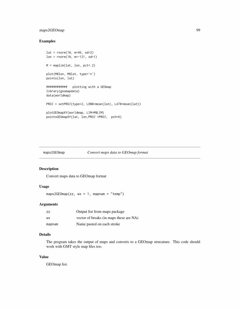
maps2GEOmap 99

Examples

lat = rnorm(10, m=46, sd=2)lon = rnorm(10, m=-121, sd=1)

M = maplim(lat, lon, pct=.2)

plot(M$lon, M$lat, type='n')points(lon, lat)

############ plotting with a GEOmaplibrary(geomapdata)data(worldmap)

PROJ = setPROJ(type=2, LON0=mean(lon), LAT0=mean(lat))

plotGEOmapXY(worldmap, LIM=M$LIM)pointsGEOmapXY(lat, lon,PROJ =PROJ, pch=6)

maps2GEOmap Convert maps data to GEOmap format

Description

Convert maps data to GEOmap format

Usage

maps2GEOmap(zz, wx = 1, mapnam = "temp")

Arguments

zz Output list from maps package

wx vector of breaks (in maps these are NA)

mapnam Name pasted on each stroke

Details

The program takes the output of maps and converts to a GEOmap strucuture. This code shouldwork with GMT style map files too.

Value

GEOmap list.

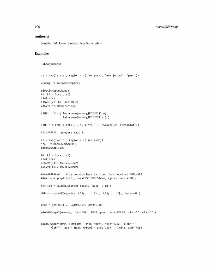
100 maps2GEOmap

Author(s)


Examples

library(maps)

zz = map('state', region = c('new york', 'new jersey', 'penn'))

neweng = maps2GEOmap(zz)

plotGEOmap(neweng)## L1 = locator(1)L1=list()L1$x=c(283.671347071854)L1$y=c(42.008587074537)

LIMS1 = list( lon=range(neweng$POINTS$lon),lat=range(neweng$POINTS$lat) )

LIMS = c(LIMS1$lon[1], LIMS1$lat[1], LIMS1$lon[2], LIMS1$lat[2])

########## prepare maps 2:

z2 = map('world', region = c('iceland'))ice = maps2GEOmap(z2)plotGEOmap(ice)

## L2 = locator(1)L2=list()L2$x=c(341.146812632372)L2$y=c(64.9180246121089)

############ this version here is nicer, but required WORLMAP2###kice = grep('ice' , coast2$STROKES$nam, ignore.case =TRUE)

### ice = GEOmap.Extract(coast2, kice ,"in")

MAP = rotateGEOmap(ice, L1$y , L1$x , L2$y , L2$x, beta=-90 )

proj = setPROJ( 2, LAT0=L1$y, LON0=L1$x )

plotGEOmapXY(neweng, LIM=LIMS, PROJ =proj, axes=FALSE, xlab="", ylab="" )

plotGEOmapXY(MAP, LIM=LIMS, PROJ =proj, axes=FALSE, xlab="",ylab="", add = TRUE, MAPcol = grey(.85) , lwd=2, xpd=TRUE)

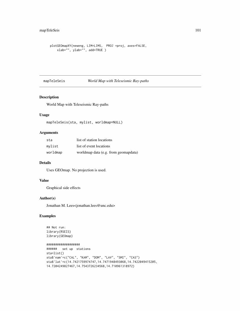
mapTeleSeis 101

plotGEOmapXY(neweng, LIM=LIMS, PROJ =proj, axes=FALSE,xlab="", ylab="", add=TRUE )

mapTeleSeis World Map with Teleseismic Ray-paths

Description

World Map with Teleseismic Ray-paths

Usage

mapTeleSeis(sta, mylist, worldmap=NULL)

Arguments

sta list of station locations

mylist list of event locations

worldmap worldmap data (e.g. from geomapdata)

Details

Uses GEOmap. No projection is used.

Value

Graphical side effects

Author(s)


Examples

## Not run:library(RSEIS)library(GEOmap)

######################### set up stationssta=list()sta$'nam'=c("CAL", "KAM", "DOM", "LAV", "SMI", "CAS")sta$'lat'=c(14.7421759974747,14.7471948493068,14.7422049415205,14.7204249827467,14.7543726234568,14.710961318972)

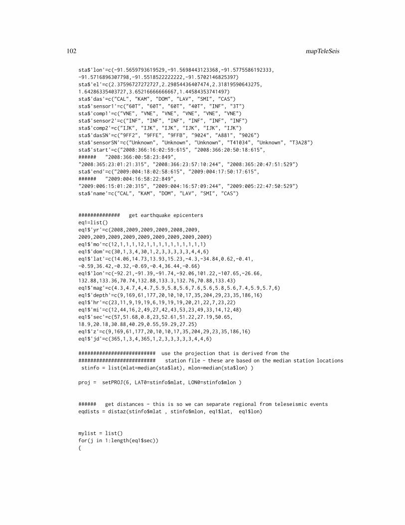
102 mapTeleSeis

sta$'lon'=c(-91.5659793619529,-91.5698443123368,-91.5775586192333,-91.5716896307798,-91.5518522222222,-91.5702146825397)sta$'el'=c(2.37596727272727,2.29854436407474,2.31819590643275,1.64286335403727,3.65216666666667,1.44584353741497)sta$'das'=c("CAL", "KAM", "DOM", "LAV", "SMI", "CAS")sta$'sensor1'=c("60T", "60T", "60T", "40T", "INF", "3T")sta$'comp1'=c("VNE", "VNE", "VNE", "VNE", "VNE", "VNE")sta$'sensor2'=c("INF", "INF", "INF", "INF", "INF", "INF")sta$'comp2'=c("IJK", "IJK", "IJK", "IJK", "IJK", "IJK")sta$'dasSN'=c("9FF2", "9FFE", "9FFB", "9024", "A881", "9026")sta$'sensorSN'=c("Unknown", "Unknown", "Unknown", "T41034", "Unknown", "T3A28")sta$'start'=c("2008:366:16:02:59:615", "2008:366:20:50:18:615",###### "2008:366:00:58:23:849","2008:365:23:01:21:315", "2008:366:23:57:10:244", "2008:365:20:47:51:529")sta$'end'=c("2009:004:18:02:58:615", "2009:004:17:50:17:615",###### "2009:004:16:58:22:849","2009:006:15:01:20:315", "2009:004:16:57:09:244", "2009:005:22:47:50:529")sta$'name'=c("CAL", "KAM", "DOM", "LAV", "SMI", "CAS")

############## get earthquake epicenterseq1=list()eq1$'yr'=c(2008,2009,2009,2009,2008,2009,2009,2009,2009,2009,2009,2009,2009,2009,2009)eq1$'mo'=c(12,1,1,1,12,1,1,1,1,1,1,1,1,1,1)eq1$'dom'=c(30,1,3,4,30,1,2,3,3,3,3,3,4,4,6)eq1$'lat'=c(14.06,14.73,13.93,15.23,-4.3,-34.84,0.62,-0.41,-0.59,36.42,-0.32,-0.69,-0.4,36.44,-0.66)eq1$'lon'=c(-92.21,-91.39,-91.74,-92.06,101.22,-107.65,-26.66,132.88,133.36,70.74,132.88,133.3,132.76,70.88,133.43)eq1$'mag'=c(4.3,4.7,4,4.7,5.9,5.8,5.6,7.6,5.6,5.8,5.6,7.4,5.9,5.7,6)eq1$'depth'=c(9,169,61,177,20,10,10,17,35,204,29,23,35,186,16)eq1$'hr'=c(23,11,9,19,19,6,19,19,19,20,21,22,7,23,22)eq1$'mi'=c(12,44,16,2,49,27,42,43,53,23,49,33,14,12,48)eq1$'sec'=c(57,51.68,0.8,23,52.61,51.22,27.19,50.65,18.9,20.18,30.88,40.29,0.55,59.29,27.25)eq1$'z'=c(9,169,61,177,20,10,10,17,35,204,29,23,35,186,16)eq1$'jd'=c(365,1,3,4,365,1,2,3,3,3,3,3,4,4,6)

########################## use the projection that is derived from the########################## station file - these are based on the median station locationsstinfo = list(mlat=median(sta$lat), mlon=median(sta$lon) )

proj = setPROJ(6, LAT0=stinfo$mlat, LON0=stinfo$mlon )

###### get distances - this is so we can separate regional from teleseismic eventseqdists = distaz(stinfo$mlat , stinfo$mlon, eq1$lat, eq1$lon)

mylist = list()for(j in 1:length(eq1$sec)){

Markup 103

mylist[[j]] = list(yr=eq1$yr[j], jd=eq1$jd[j], mo=eq1$mo[j], dom=eq1$dom[j], hr=eq1$hr[j],mi=eq1$mi[j], sec=eq1$sec[j], lat=eq1$lat[j], lon=eq1$lon[j], z=eq1$z[j], mag=eq1$mag[j])}

library(geomapdata)data(worldmap)

mapTeleSeis(sta, mylist, worldmap=worldmap)

## End(Not run)

Markup Add markup information to an existing plot

Description

For use in GEOmap to add labels to a geographic plot

Usage

Markup(MM = list(), sel = 1, cex = 1, ...)

Arguments

MM list of markup infromation

sel vector, select which marks to be plotted

cex character expansion

... graphical parameters for par

Details

Uses the locator function

Value


104 merid

Author(s)


See Also

setMarkup, plotGEOmapXY

Examples

## Not run:

plot(c(0, 1), c(0, 1), main = "this is a test", sub = "sutitle",xlab = "this is x", ylab = "this is y")

LABS = c("this is", "a", "test")

MUP = setMarkup(LABS)

## End(Not run)

merid Orthogonal Projection of Meridian or Parallel

Description

Orthogonal Projection Meridian or Parallel

Usage

merid(lon, lat1=-90, lat2=90, lam0=0, phi1=41, R=1, by=1)paral(lat, lon1=-180 , lon2=180, lam0=0, phi1=41, R=1, by=1)

Arguments

lon merid starting Longitude, degrees

lat paral starting Latitude, degrees

lam0 origin Longitude, degrees

phi1 origin Latitude, degrees

R Radius

by increment in degrees

lat1 merid starting Latitude, degrees

merid 105

lat2 merid ending Latitude, degrees

lon1 paral starting Longitude, degrees

lon2 paral ending Longitude, degrees

Details

Retruns points along a meridian running through lat, lon with a projection based on lam0 phi.

Value

list of x-y values for plotting

Author(s)


References


See Also

ortho.proj

Examples

olat = 0olon = 0

tlat = 23tlon = 30

M = merid(tlon, lat1=tlat, olon, olat, 1)

R = 1

phi1=40

GLOBE.ORTH(20, phi1, 1,plotmap=FALSE)

M1 = merid(20, lat1=20, lat2=40, phi1=phi1, lam0=olat, R=1, by=1)

P2 = paral(40, lon1=20 , lon2=40, lam0=olat, phi1=phi1, R=1, by=1)

M2 = merid(40, lat1=40, lat2=20, phi1=phi1, lam0=olat, R=1, by=1)

P1 = paral(20, lon1=40 , lon2=20, lam0=olat, phi1=phi1, R=1, by=1)

106 niceLLtix

polygon(c(M1$x, P2$x, M2$x, P1$x), c(M1$y, P2$y, M2$y, P1$y),col=rgb(.8, .8, 1))

niceLLtix Nice DMS coordinates

Description

Determine a nice set of coordinates in DMS

Usage

niceLLtix(rcoords)

Arguments

rcoords vector of decimal degrees, the range will be used

Value

DD decimal degrees

deg degrees

min minutes

sec seconds

si sign of degrees

Author(s)


See Also

dms

Examples

niceLLtix(c(12.5, 12.58) )niceLLtix(c(12.57, 12.58) )

niceLLtix(c(91.5, 92.8) )niceLLtix(c(-91.5, -92.8) )

niceLLtix(c(91.5, 93.8) )

NoOverlap 107

niceLLtix(c(91.5, 95.8) )

niceLLtix(c(-91.5, -95.8) )

NoOverlap Shift Symbols

Description

Shift Symbols such that there is no overlap

Usage

NoOverlap(x, y, focsiz, SEL = 0, OLDx = 0, OLDy = 0, cenx = 0, ceny = 0)

Arguments

x x-location

y y-location

focsiz symbol size

SEL selection of which symbols to shift

OLDx x-locations of origin

OLDy y-locations of origin

cenx center x

ceny center y

Details

Program is used for finding positions for exploding. A vector is dcalculated from each origin toeach point and explosions are projected along these directions until a position is found that doesnot overlap. The position is nudged by a value of focsiz at each step. If OLDx and OLDy are notprovided, cenx and ceny are used as origin points.

Value

x,y list of new positions

Author(s)


See Also

ExplodeSymbols

108 normalfault

Examples

draw.circ<-function (x, y, r, ...){

CI = RPMG::circle(1)for (i in 1:length(x)) {

Cx = x[i] + r * CI$xCy = y[i] + r * CI$ylines(c(Cx, Cx[1]), c(Cy, Cy[1]), type = "l", ...)

}}

x = rnorm(20)y = rnorm(20)

rx = range(x)ry = range(y)

drx = diff(rx)dry = diff(ry)XPCT=.2rx = c(rx[1]-XPCT*drx, rx[2]+XPCT*drx)ry = c(ry[1]-XPCT*dry, ry[2]+XPCT*dry)

plot(rx , ry , type='n', asp=1, xlab="km", ylab="km")

u = par("usr")

focsiz = 0.04* (u[2]-u[1])

draw.circ(x, y, focsiz, col='red')NXY = NoOverlap(x,y,focsiz)

plot(rx , ry , type='n', asp=1, xlab="km", ylab="km")

u = par("usr")

focsiz = 0.04* (u[2]-u[1])

draw.circ(NXY$x, NXY$y, focsiz, col="blue" )

segments(x,y,NXY$x, NXY$y)

normalfault Normal Fault trace

normalfault 109

Description

Plot normal fault on map.

Usage

normalfault(x, y, h = 1, hoff = 1, rot = list(cs = 1, sn = 0), col = "black")

Arguments

x x-coordinates

y y-coordinates

h radius of ball

hoff distance from line

rot rotation vectors, (cosines and sines)

col color

Details

Rotation vector is provided as list(cs=vector(), sn=vector()).

Value


Author(s)


See Also

GEOsymbols

Examples

G=list()G$x=c(-1.0960,-0.9942,-0.8909,-0.7846,-0.6738,-0.5570,-0.4657,-0.3709,-0.2734,-0.1740,-0.0734, 0.0246, 0.1218, 0.2169, 0.3086, 0.3956, 0.4641,0.5293, 0.5919, 0.6530, 0.7131)G$y=c(-0.72392,-0.62145,-0.52135,-0.42599,-0.33774,-0.25896,-0.20759,-0.16160,-0.11981,-0.08105,-0.04414,-0.00885, 0.02774, 0.06759, 0.11262,0.16480, 0.21487, 0.27001, 0.32895, 0.39044, 0.45319)

plot(G$x, G$y, type='n',asp=1, axes=FALSE, xlab='', ylab='')


110 NSarrow

sk = 2lines(G$x,G$y,col='blue')

bcars(g$x,g$y, h1=sk, h2=sk*.5, g$rot, col='black', border='black' )

NSarrow North-South Weather Vane Arrow

Description

Add north-south weather vane arrow figure

Usage

NSarrow(x = NULL, y = NULL, R = 1, col.arrow = 1, col.N = 1,col.circ = 1, rot = 0, PMAT = NULL)

Arguments

x X-location vector, if list, include both x and y values

y Y-location vector, not needed if x is a list

R radius, in plot coordinates

col.arrow color for arrow, default="black"

col.N color for N symbol

col.circ color for circle

rot rotation angle, degrees

PMAT projection matrix, output of persp

Details

The location list should have 2 values for x and y each, the second value for y determines the radiusR if it is not provided. The first element of y is the center of the weather vane. If no x-list isprovided, the interactive locator function is invoked and a list is returned for future work.

Value

x x-location

y y-location

Author(s)


See Also

zebra

NSWath 111

Examples

plot(c(1:10), c(1:10), type='n')

x=c(2,2)y = c(8,9)

NSarrow(list(x=x, y=y))

##### move over and repeat, with rotation of 25 degrees west

x=c(5,5)y = c(8,9)

NSarrow(list(x=x, y=y), rot=25)

NSWath Cross sectional Swaths of Earthquakes over Japan

Description

Set of 4 swaths for cross section across Japan

Usage

data(NSWath)

Format

list of cross sections each conists of a list of form:

r r-distance along cross section (x-coordinate)

dh distance from cross seection

depth depth in cross section (y-coordinate)

flag index vector of which earthquakes fell in swath and depth range

InvBox coordinates of swath for plotting on map

Source

Data is extrcted from an earthquake data base of relocated events provided by Robert Engdahl.

112 ortho.proj

References

Engdahl, E. R., R. D. van der Hilst, S. H. Kirby, G. Ekstrom, K. M. Shedlock, and A. F. Sheehan(1998), A global survey of slab structures and internal processes using a combined data base ofhigh-resolution earthquake hypocenters, tomographic images and focal mechanism data, Seismol.Res. Lett., 69, 153-154.

Examples

## Not run:data(NSWath)for(i in 1:length(NSWath)){dev.new()LAB = attr(NSWath[[i]], "LAB")

XSECwin( NSWath[[i]] , iseclab=i, xLAB=LAB , labs=NULL, demo=TRUE )}

## End(Not run)

ortho.proj Orthogonal Map Projection

Description

Orthogonal Map Projection

Usage

ortho.proj(lat, lon, lon0, lat1, R)

Arguments

lat latitude, degrees

lon longitude, degrees

lon0 view origin longitude, degrees

lat1 view origin latitude, degrees

R Radius of sphere, default=1

Details

Assumes spherical globe. This function is not part of the normal GEOmap plotting routines.

OverTurned 113

Value

list

x x, coordinate in units of R

y y, coordinate in units of R

Author(s)


References


See Also

GLOBE.ORTH, setPROJ, projtype

Examples

olat = 0olon = 0

tlat = 23tlon = 30

R = 1ortho.proj(tlat, tlon, olon, olat, R)

OverTurned Plot Overturned fault

Description

Plot Overturned fault

Usage

OverTurned(x, y, syn = TRUE, spacing = NULL, N = 1, r1 = 1, r2 = 1.2,h1 = 0.5, h2 = 0.5, endtol = 0.1, REV = FALSE, col = "black", ...)

114 OverTurned

Arguments

x x-coordinates

y y-coordinates

syn logical, TRUE=syncline, FALSE=anticline

spacing spacing of points

N number of points






REV reverse direction of x-y


... graphical parameters

Value


Author(s)


See Also

PointsAlong

Examples


OverTurned(ff$x,ff$y, r1= .4, r2= .8, h1= .5, h2= .5, N=5, syn=FALSE,endtol=.2)

perpen 115

perpen perpendicular marks along line

Description

draw perpendicular marks along line

Usage

perpen(x, y, h, rot, col = "black", lwd = 1)

Arguments

x x-coordinates

y y coordinates

h height of tooth

rot rotation of teeth

col color of line

lwd line width

Details

Used by faultperp

Value

graphical side effects

Author(s)


See Also

PointsAlong, faultperp

Examples



lines(G)

116 pgon

perpen(g$x, g$y, .3, g$rot, col = "black", lwd = 1)

pgon Plot regular polygon: pentagon, hexagon, octagon

Description

Plot regular polygon: pentagon, hexagon, octagon

Usage

pgon(x, y, siz=siz, col="black", border=NULL, K=5, startalph = -45, ... )

Arguments

x x-coordinate

y y-coordinate

siz radius or size

col inside color

border border color

K number of sides per polygon

startalph starting angle


Details

I figure is resized needs to be re-called.

Value


Author(s)


pline 117

Examples

N = 25x = rnorm(N)y = rnorm(N)

z = rnorm(N)

######## draw pentagonsplot(x,y, type='n', axes=FALSE, ann=FALSE)pgon(x,y, siz=abs(z)/10, col="white", border='black', startalph =60, K=5, lwd=.5, xpd=TRUE)

###### color the points, use 4-sided blocksrbow=rainbow(100)

ss = sample(1:100, N, replace = TRUE, prob = NULL)plot(x,y, type='n', axes=FALSE, ann=FALSE)pgon(x,y, siz=abs(z)/10, col=rbow[ss], border='black', startalph =60, K=4, lwd=.5, xpd=TRUE)

pline Point to line distance

Description

get sortest distance from arbitrary point to a segment.

Usage

pline(x1, y1, x2, y2, ex, ey)

Arguments

x1 x coordinate segment start

y1 y coordinate segment start

x2 x coordinate segment end

y2 y coordinate segment end

ex x, point

ey y point

118 plotGEOmap

Value

vector of:

dis distance to segmentdee distance to linezee projection along linepx x, point of intersectionpy y, point of intersection

Author(s)


See Also

polyintern

Examples

L=list()L$x=c(-0.161416832868, 0.484046270443,-0.472622257679)L$y=c(-0.735779816514, 0.306422018349, 0.192660550459)

P = pline(L$x[1], L$y[1], L$x[2], L$y[2], L$x[3], L$y[3])

plot(L$x, L$y, type='n', asp=1)segments(L$x[1], L$y[1], L$x[2], L$y[2])points( L$x[3], L$y[3])

segments(L$x[3], L$y[3], P[4], P[5], col='red')

plotGEOmap Plot a GEO map

Description

High Level plot of GEO map

Usage

plotGEOmap(MAP, LIM = c(-180, -90, 180, 90) ,shiftlon = 0, add = TRUE ,NUMB = FALSE , SEL = NULL, MAPcol = NULL,MAPstyle = NULL, border=NA,PLOT = TRUE, PRINT=FALSE, BB = FALSE, ...)

plotGEOmap 119

Arguments

MAP Map Structure

LIM Lat-Lon limits

add logical, TRUE= add to existing plot

SEL Index vector of strokes to be used in plotting, default=NULL(use all that passother tests)

MAPcol override color for maps

MAPstyle override plotting style for maps

border color, add border to polygons, NA=no border

shiftlon degrees, rotate longitude

NUMB logical, number the strokes on the map

PLOT logical, TRUE=plot map, else just set up plotting area

PRINT logical, TRUE=show selected stroke indeces on the screen(default=FALSE)

BB logical, TRUE=add bounding box to each stroke (default=FALSE)


Details

plotGEOmap does not plot a projected map. MAPcol and MAPstyle can be used to override thecolors and style in the map-list. These are applied to all the strokes.

Value


Author(s)


See Also

plotGEOmapXY, DOTOPOMAPI, addLLXY

Examples

library(geomapdata)

data(coastmap)

plotGEOmap(coastmap , xaxs='i', yaxs='i')

#################### example:coastmap$STROKES$col[coastmap$STROKES$code=="C" ] = rgb(1, .6, .6)coastmap$STROKES$col[coastmap$STROKES$code=="c" ] = rgb(1, .9, .9)coastmap$STROKES$col[coastmap$STROKES$code=="L" ] = rgb(.6, .6, 1)

120 plotGEOmapXY

plot(c(-30, 370), c(-85, 85), type='n', ann=FALSE, xaxs='i', yaxs='i')

plotGEOmap(coastmap , border='black' , add=TRUE)title(xlab="Longitude", ylab="Latitude" )grid()

box()

## Not run:

### political map of the worldlibrary(geomapdata)plotGEOmap(coastmap , border='black' , add=FALSE, xaxs='i')

data(europe.bdy)data(asia.bdy)

data(africa.bdy)data(namer.bdy)

data(samer.bdy)data(USAmap)

plotGEOmap(europe.bdy , add=TRUE)plotGEOmap(asia.bdy , add=TRUE)plotGEOmap(africa.bdy , add=TRUE)plotGEOmap(namer.bdy , add=TRUE)

plotGEOmap(samer.bdy , add=TRUE)

plotGEOmap(USAmap , add=TRUE)

## End(Not run)

plotGEOmapXY Plot a projected GEO map

Description

High Level plot of GEO map

plotGEOmapXY 121

Usage

plotGEOmapXY(MAP, LIM = c(-180, -90, 180, 90),PROJ = list(), PMAT=NULL,add = TRUE, SEL=NULL , GRID = NULL, GRIDcol = 1,MAPcol = NULL, MAPstyle = NULL, border = NA,cenlon = 0, shiftlon = 0, linelty = 1,linelwd = 1, ptpch=".", ptcex=1, NUMB = FALSE, ...)

Arguments

MAP Map Structure

LIM Lat-Lon limits

PROJ Projection list


add logical, TRUE= add to existing plot

SEL Index vector of strokes to be used in plotting, default=NULL(use all that passother tests)

GRID logical, TRUE=add grid lines

GRIDcol color for grid lines

MAPcol override color for maps

MAPstyle override plotting style for maps

border color, add border to polygons, NA=no border

cenlon center longitude of plot

shiftlon degrees, rotate longitude

linelty Line type

linelwd line width

ptpch plotting character for strokes (style=1) that are plotted as points

ptcex character expansion factor for style=1 strokes

NUMB logical, number the strokes on the map


Details

plotGEOmapXY includes projection of the data, plotGEOmap does not. MAPcol and MAPstylecan be used to override the colors and style in the map-list. These are applied to all the strokes.

For strokes that are of style=1 points are plotted with graphical parameters ptpch="." and ptcex=1unless otherwise indicated.

Value


122 plothypos

Author(s)


See Also

DOTOPOMAPI, addLLXY, plotGEOmap

Examples

data('japmap', package='geomapdata' )isel1 = which( japmap$STROKES$code != "i" & japmap$STROKES$num>120 )

PLOC=list(LON=c(137.008, 141.000), LAT=c(34.000, 36.992),x=c(137.008, 141.000), y=c(34.000, 36.992) )

PROJ = setPROJ(type=2, LAT0=mean(PLOC$y) , LON0=mean(PLOC$x) )

gxy = GLOB.XY(PLOC$LAT, PLOC$LON, PROJ)PLAT = pretty(PLOC$LAT)

PLAT = c(min(PLOC$LAT),PLAT[PLAT>min(PLOC$LAT) & PLAT<max(PLOC$LAT)],max(PLOC$LAT))

PLON = pretty(PLOC$LON)PLON = c(min(PLOC$LON),

PLON[PLON>min(PLOC$LON) & PLON<max(PLOC$LON)], max(PLOC$LON))

plot(gxy$x, gxy$y, asp=TRUE, ann=FALSE , axes=FALSE)

plotGEOmapXY(japmap,SEL=isel1, LIM=c(PLOC$LON[1], PLOC$LAT[1],PLOC$LON[2],PLOC$LAT[2]) , PROJ=PROJ, add=TRUE )

addLLXY(PLAT, PLON, PROJ=PROJ, LABS=TRUE, PMAT=NULL, TICS=c(.1,.1) )

################### rotated mapPMAT = rotdelta4(-34)

plotGEOmapXY(japmap, PMAT=PMAT,SEL=isel1, xpd=TRUE)

plothypos Plot Edicenters

Description

Plot hypocenter color coded to depth and size scaled by magnitude.

plothypos 123

Usage

plothypos(lat, lon, z, proj, mag = NULL, cex = 0.4, pch =21, PMAT = NULL, alpha = NULL)

Arguments

lat Latitude

lon Longitude

z km Depth, (positive down)

proj Projection structure

mag Magnitude


pch plotting character, default=21

PMAT transformation matrix

alpha transparency factor

Details

Adds hypocenters to an existing plot.

Value

Graphical Side effects.

Note

The events are color coded according to depth.

Only a few devices can handle transparency effects.

Author(s)


See Also

plotGEOmapXY, XSECEQ, eqswath, getmagsize

Examples

library(geomapdata)

data('EHB.LLZ')data('japmap', package='geomapdata')

RLAT = range(japmap$POINTS$lat)RLON = range(japmap$POINTS$lon)

JLAT = expandbound(RLAT, .1)

124 plothypos

JLON = expandbound(RLON, .1)

PROJ = japmap$PROJ############## select the events in the regionisel1 = which( japmap$STROKES$code != "i" & japmap$STROKES$num>120 )

sel = which(EHB.LLZ$lat > JLAT[1] &EHB.LLZ$lat < JLAT[2] &EHB.LLZ$lon > JLON[1] &EHB.LLZ$lon < JLON[2])

sel = sel[1:200]

plotGEOmapXY(japmap , PROJ=PROJ, SEL=isel1, add=FALSE, MAPcol="black")

plothypos(EHB.LLZ$lat[sel], EHB.LLZ$lon[sel], EHB.LLZ$z[sel], PROJ,mag=NULL, cex=.8)

## Not run:

fn = "/home/lees/WORK/SENDAI.EVENT/catsearch.8757"

g = getANSS(fn, skip=2)g$jd = getjul(g$yr, g$mo, g$dom)

sel = which(g$lat > JLAT[1] &g$lat < JLAT[2] &g$lon > JLON[1] &g$lon < JLON[2])

olat = g$lat[sel]olon = g$lon[sel]ordz = g$z[sel]

mag = g$mag[sel]

gm = getmagsize(mag)

plotGEOmapXY(japmap , PROJ=PROJ, add=FALSE, MAPcol="black")plothypos(g$lat[sel], g$lon[sel], g$z[sel], PROJ,mag=NULL, cex=gm)

plotGEOmapXY(japmap , PROJ=PROJ, add=FALSE, MAPcol="black")plothypos(olat, olon, ordz, PROJ,mag=NULL, cex=gm)

plotGEOmapXY(japmap , PROJ=PROJ, add=FALSE, MAPcol="black")

plotnicetix 125

plothypos(olat, olon, ordz, PROJ,mag=mag, cex=1 )

################## transparent plotpdfname = local.file('TOHOKU', "pdf")

cairo_pdf(file = pdfname , width = 8, height = 10)plotGEOmapXY(japmap , PROJ=PROJ, add=FALSE, MAPcol="black")plothypos(olat, olon, ordz, PROJ,mag=mag, cex=1, alpha=.3 )dev.off()##################

## End(Not run)

plotnicetix Plot Lat-Lon tick marks

Description

Find and plot nice tick marks on projected plot

Usage

plotnicetix(nex, nwhy, proj, tlen = 0.1,fonts = c("serif", "plain"), PMAT = NULL, PLOT = TRUE)

Arguments

nex X coordinates

nwhy Y coordinates

proj prjection list

tlen length for tic marks (inches)

fonts Hershy font vector

PMAT projection matrix from persp

PLOT logical, TRUE = add to plot

126 plotusa

Value


Author(s)


See Also

niceLLtix, goodticdivs, getnicetix, dms

Examples

proj = setPROJ(7, LAT0 = 0 , LON0= -93)

rx = c(652713.4, 656017.4)ry = c(1629271, 1631755)

plot(rx, ry, type='n', asp=1, axes=FALSE , ann=FALSE)plotnicetix(rx, ry, proj, PMAT=NULL)

plotusa Map of USA

Description

Quick plot of USA project with UTM.

Usage

plotusa(USAmap, LATS=c(22,49.62741), LONS=c(229.29389,296.41803), add=FALSE)

Arguments

USAmap Map for the U.S. (from geomapdata)

LATS vector of latitude bounds

LONS vector of longitude bounds

add add to existing plot

Value

Graphical Side Effect

plotUTM 127

Author(s)


See Also

zebra

Examples

## Not run:library(geomapdata)data(package='geomapdata', "USAmap")plotusa(USAmap)

## End(Not run)

plotUTM Plot UTM

Description

Plot UTM

Usage

plotUTM(proj, LIM, shiftlon = 0)

Arguments

proj projection

LIM Limit vector

shiftlon rotation around z axiz, default=0

Value


Author(s)


See Also

GLOB.XY

128 plotworldmap

Examples

library(geomapdata)

data(USAmap)

proj = setPROJ(type=3, LAT0=33.75, LON0= RPMG::fmod(-79., 360) ,LAT1=34.333333, LAT2=36.166667, LATS=NULL, LONS=NULL,DLAT=NULL, DLON=NULL,FE=0,FN=0)

ALOC=list(lon=c(274.5,288), lat=c(31, 38),LON=c(274.5, 288), LAT=c(31, 38), shiftlon=0)

plotGEOmapXY(USAmap, LIM=c(ALOC$LON[1], ALOC$lat[1],ALOC$LON[2], ALOC$lat[2]) , PROJ=proj, add=FALSE, shiftlon=0)

plotUTM(proj, c(ALOC$LON[1], ALOC$lat[1], ALOC$LON[2], ALOC$lat[2]))

############## larger scale


data(USAmap)

p = plotusa(USAmap)

plotUTM(p$PROJ, LIM=p$LIM)

## End(Not run)

plotworldmap Plot World Map with UTM sections

Description

Plot World Map with UTM sections

Usage

plotworldmap(MAP, LIM = c(-180, -90, 180, 90), shiftlon = 0,add = TRUE, NUMB = FALSE, ...)

PointsAlong 129

Arguments

MAP GEOmap structure

LIM vector of limits c(lon1, lat1, lon2, lat2)


add logical, TRUE=add to current plot

NUMB logical, add numbers to plot

... grpahical parameters from par

Value


Author(s)


See Also

plotGEOmap, plotGEOmapXY

Examples

library(geomapdata)data(worldmap)plotworldmap(worldmap)

PointsAlong Find spaced Points along a line

Description

find evenly spaced points along a line

Usage

PointsAlong(x, y, spacing = NULL, N = 1, endtol = 0.1)

Arguments

x x-coordinates

y y-coordinates


N number of points


130 polyintern

Details

The total length is returned: this is the line integral along the trace.

Value

List:

x x-coordinates

y y-coordinates

rot angle at the points

TOT total length along the trace

Author(s)


Examples


g = PointsAlong(ff$x, ff$y, N=20)

lines(ff$x, ff$y)points(g$x, g$y)

polyintern Internal point of polygon

Description

Find a central internal point of a polygon

Usage

polyintern(P, n = 10, PLOT=FALSE)

Arguments

P Polygon,xy

n grid dimension over polygon, n by n

PLOT logical, TRUE=plot

printGEOinfo 131

Details

A grid is laid over the polygo, the internal points are extracted and for each one the shortest distanceto te perimeter is determined. Then the point with the largest distance is returned.

Value

x x coordinate of point

y y coordinate of point

zi index of point

nx internal grid points x

ny internal grid points y

ef internal grid points distances to perimeter

Author(s)


See Also

pline

Examples

X=list()X$x=c(11.991,11.942,11.891,11.834,11.775,11.725,11.691,

11.712,11.746,11.804,11.865,11.957,11.991)X$y=c(-2.0091,-2.0699,-2.0823,-2.1091,-2.1419,

-2.1394,-2.1165,-2.0604,-2.0196,-1.9847,-1.9668,-1.9777,-2.0091)

polyintern(X, n = 10, PLOT=TRUE)

printGEOinfo printGEOinfo

Description

Print information on GEOmap strokes

Usage

printGEOinfo(MAP, kstroke)

132 printGEOmap

Arguments

MAP GEOmap

kstroke index to strokes

Details

Prints some of the meta data stored in the GEOmap header list, strokes.

Value

Side Effects

Author(s)


See Also

printGEOmap

Examples

data(coastmap)printGEOinfo(coastmap, 1:10)

printGEOmap printGEOmap

Description

Print information on GEOmap strokes

Usage

printGEOmap(G)

Arguments

G GEOmap

Details

Prints the full STROES list as a dataframe.

Value

Side Effects

projtype 133

Author(s)


See Also

printGEOinfo

Examples

data(coastmap)printGEOmap(coastmap)

projtype List of Projection types

Description

List of Projection types in GEOMAP

Usage

projtype(proj=list())

Arguments

proj Projection list

Details

Just returns possile choices.

Value

Side Effects

Author(s)


References


See Also

setPROJ

134 rectPERIM

Examples

projtype()


projtype(proj)

## or, for Kamchatka-AleutiansLL=c(54.3861210149126,171.626386683545)

PROJ = setPROJ(type=2, LAT0=LL[1], LON0=LL[2], LATS=NULL, LONS=NULL, DLAT=NULL, DLON=NULL, FN =0)projtype(PROJ)

rectPERIM Extract a rectangular perimeter

Description

Extract a rectangular perimeter

Usage

rectPERIM(x, y = 1, pct = 0)

Arguments

x x values or a list include x, y members

y y values, if missing, x must be a list

pct Percent expansion, based on range of x and y values. If pct>1 it is divided by100 to get a fractional percent expansion.

Details

The rectangular box will be expanded based on the percent pct.

Value

list of x, y values from lower left corner counter clockwise around perimeter

Author(s)


See Also

getGEOperim

rekt2line 135

Examples

fx =rnorm(20)fy = rnorm(20)

plot(fx, fy, xlim=c(-4, 4), ylim=c(-4,4))rp = rectPERIM(fx, fy)

polygon(rp)text(rp, labels=1:4, pos=c(1,1,3,3), font=2, cex=2)

fx2 =rnorm(20, m=-1)fy2 = rnorm(20, m=-1)

Fx = list(x=fx2, y=fy2)

points(Fx$x, Fx$y, col='red')

rp = rectPERIM(Fx)

polygon(rp, border='red')

######## try expanding the perim:

plot(fx, fy, xlim=c(-4, 4), ylim=c(-4,4), asp=1)rp = rectPERIM(fx, fy, pct=0.1)

polygon(rp)

rp = rectPERIM(fx, fy, pct=0.2)

polygon(rp)

rekt2line Rectangle Line Overlap

Description

Find points on a rectangle closest to a set of points.

Usage

rekt2line(rekt, pnts)

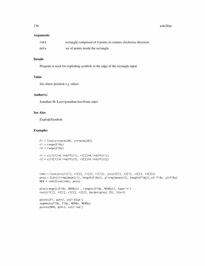
136 rekt2line

Arguments

rekt rectangle comprised of 4 points in counter clockwise direction.

pnts set of points inside the rectangle

Details

Program is used for exploding symbols to the edge of the rectangle input

Value

list ofnew poistion x,y values

Author(s)


See Also

ExplodeSymbols

Examples

F1 = list(x=rnorm(20), y=rnorm(20))r1 = range(F1$x)r2 = range(F1$y)

r1 = c(r1[1]-0.1*diff(r1), r1[2]+0.1*diff(r1))r2 = c(r2[1]-0.1*diff(r2), r2[2]+0.1*diff(r2))

rekt = list(x=c(r1[1], r1[2], r1[2], r1[1]), y=c(r2[1], r2[1], r2[2], r2[2]))pnts = list(x1=rep(mean(r1), length(F1$x)), y1=rep(mean(r2), length(F1$y)),x2= F1$x, y2=F1$y)NEW = rekt2line(rekt, pnts)

plot(range(c(F1$x, NEW$x)) , range(c(F1$y, NEW$y)), type='n')rect(r1[1], r2[1], r1[2], r2[2], border=grey(.75), lty=2)

points(F1, pch=2, col='blue')segments(F1$x, F1$y, NEW$x, NEW$y)points(NEW, pch=3, col='red')

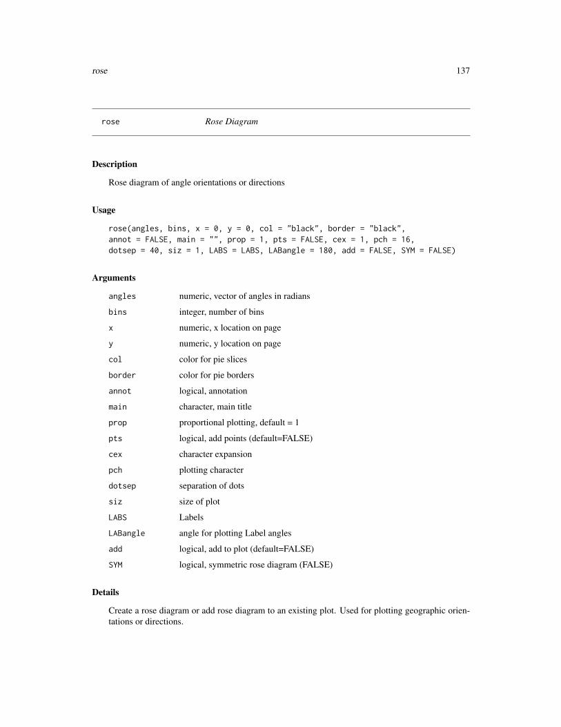
rose 137

rose Rose Diagram

Description

Rose diagram of angle orientations or directions

Usage

rose(angles, bins, x = 0, y = 0, col = "black", border = "black",annot = FALSE, main = "", prop = 1, pts = FALSE, cex = 1, pch = 16,dotsep = 40, siz = 1, LABS = LABS, LABangle = 180, add = FALSE, SYM = FALSE)

Arguments

angles numeric, vector of angles in radians

bins integer, number of bins

x numeric, x location on page

y numeric, y location on page

col color for pie slices

border color for pie borders

annot logical, annotation

main character, main title

prop proportional plotting, default = 1

pts logical, add points (default=FALSE)


pch plotting character

dotsep separation of dots

siz size of plot

LABS Labels

LABangle angle for plotting Label angles

add logical, add to plot (default=FALSE)

SYM logical, symmetric rose diagram (FALSE)

Details

Create a rose diagram or add rose diagram to an existing plot. Used for plotting geographic orien-tations or directions.

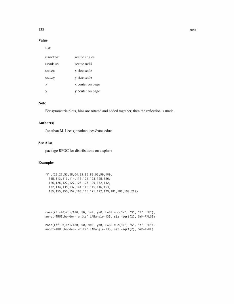
138 rose

Value

list:

usector sector angles

uradius sector radii

usizx x size scale

usizy y size scale

x x center on page

y y center on page

Note

For symmetric plots, bins are rotated and added together, then the reflection is made.

Author(s)


See Also

package RFOC for distributions on a sphere

Examples

ff=c(23,27,53,58,64,83,85,88,93,99,100,105,113,113,114,117,121,123,125,126,126,126,127,127,128,128,129,132,132,132,134,135,137,144,145,145,146,153,155,155,155,157,163,165,171,172,179,181,186,190,212)

rose((ff-90)*pi/180, 50, x=0, y=0, LABS = c("N", "S", "W", "E"),annot=TRUE,border='white',LABangle=135, siz =sqrt(2), SYM=FALSE)

rose((ff-90)*pi/180, 50, x=0, y=0, LABS = c("N", "S", "W", "E"),annot=TRUE,border='white',LABangle=135, siz =sqrt(2), SYM=TRUE)

rotateGEOmap 139

rotateGEOmap Rotate a GEOmap

Description

Rotate a GEOmap to a new location on the globe

Usage

rotateGEOmap(INmap, TARGlat, TARGlon, LAT0, LON0, beta = 0)

Arguments

INmap Input GEOmap

TARGlat Target center latitide

TARGlon Target center longitide

LAT0 Source center latitide

LON0 Source center longitide

beta rotation through axis coming out of screen

Details

This function is used to translate a given map region to another for over plotting. You can comparethe areas of two region using the same projection.

Value

GEOmap list.

Author(s)


See Also

plotGEOmapXY

Examples

library(maps)

zz = map('state', region = c('new york', 'new jersey', 'penn'))

neweng = maps2GEOmap(zz)

plotGEOmap(neweng)

140 rotdelta4


LIMS1 = list( lon=range(neweng$POINTS$lon), lat=range(neweng$POINTS$lat) )

LIMS = c(LIMS1$lon[1], LIMS1$lat[1], LIMS1$lon[2], LIMS1$lat[2])

########## prepare maps 2:

z2 = map('world', region = c('iceland'))ice = maps2GEOmap(z2)plotGEOmap(ice)


############ this version here is nicer, but required WORLMAP2###kice = grep('ice' , coast2$STROKES$nam, ignore.case =TRUE)

### ice = GEOmap.Extract(coast2, kice ,"in")

MAP = rotateGEOmap(ice, L1$y , L1$x , L2$y , L2$x, beta=-90 )

proj = setPROJ( 2, LAT0=L1$y, LON0=L1$x )

plotGEOmapXY(neweng, LIM=LIMS, PROJ =proj, axes=FALSE, xlab="", ylab="" )

plotGEOmapXY(MAP, LIM=LIMS, PROJ =proj, axes=FALSE, xlab="",ylab="", add = TRUE, MAPcol = grey(.85) , lwd=2, xpd=TRUE)

plotGEOmapXY(neweng, LIM=LIMS, PROJ =proj,axes=FALSE, xlab="", ylab="", add=TRUE )

rotdelta4 rotation about Z-axis

Description

rotation about Z-axis

rotmat2D 141

Usage

rotdelta4(delta)

Arguments

delta angle in degrees

Value

Matrix for rotation

Author(s)


See Also

roty4, rotx4, trans4

Examples

rotdelta4(23)

rotmat2D set a rotation matrix

Description

set a rotation matrix

Usage

rotmat2D(alph)

Arguments

alph angle in radians

Value

matrix for rotation in 2 dimensions

Author(s)


142 rotx4

Examples

######## make an ellipsetheta=seq(0,360,by=5)*pi/180

r1 = 0.4r2 = 0.2

m=matrix(rep(0,2*length(theta)),ncol=2)

m[,1]=r1*cos(theta)m[,2]=r2*sin(theta)

## make a dummy plot and draw ellipse


lines(m[,1]+.5, m[,2]+.5)

## get rotation matrixR = rotmat2D(32)

######### apply rotationnm=m %*% R

### plotlines(nm[,1]+.5, nm[,2]+.5, col='red')

rotx4 x-axis rotation matrix

Description

x-axis rotation matrix

Usage

rotx4(vec)

Arguments

vec vector of direction cosines

roty4 143

Details

Length of vector cannot be zero.

Value

Matrix for rotation

Author(s)


See Also

roty4, rotdelta4

Examples

v = c(12,13,-4)

rotx4(v)

roty4 y-axis rotation matrix

Description

y-axis rotation matrix

Usage

roty4(vec)

Arguments

vec vector of direction cosines

Details

Length of vector cannot be zero.

Value

Matrix for rotation

144 SELGEOmap

Author(s)


References

Rogers and Adams

See Also

rotx4, rotdelta4

Examples

v = c(12,13,-4)

roty4(v)

SELGEOmap Select parts of a GEOmap

Description

Using area, number of points and Lat-Lon Limits, extracts map strokes and creates a new GEOmap

Usage

SELGEOmap(MAP, ncut = 3, acut = c(0, 1e+05), proj = NULL, LIM = NULL)

Arguments

MAP Map structure

ncut minimum number of points in polygon

acut vector, min and max of areas to include

proj map projection

LIM vector, c(lon1, lat1, lon2, lat2)

Details

Uses splancs function. If proj and LIM are NULL then no selection on limits are used ncut is usedto eliminate area calculations with strokes less than the specified number.

SELGEOmap 145

Value

GEOmap LIST

STROKES list

nam name of stroke

num number of points in stroke

index index of stroke

col color of stroke

style style of stroke

code code of stroke

LAT1 lower left Lat of stroke

LAT2 upper right Lat of stroke

LON1 lower left Lon of stroke

LON2 upper right Lon of stroke

POINTS list

lat vector of lats

lon vector of lons

Author(s)


See Also

geoarea

Examples

library(geomapdata)data(worldmap)skam = SELGEOmap(worldmap, ncut=3, acut=c(10000, Inf), proj=NULL, LIM=NULL)

par(mfrow=c(2,1))

####### plot world map, with all lines:plotGEOmap(worldmap)length(worldmap$STROKES$num)###### same plot with some lines removed:plotGEOmap(skam)length(skam$STROKES$num)

##########################################

146 setMarkup

setMarkup Set up mark up for maps

Description

Interactive set up of mark of labels for a map

Usage

setMarkup(LABS = NULL, PROJ = NULL)

Arguments

LABS vector of labels


Details

labels are set one-by-one and the user inout relevant information like locator() and other features

Value

List of Markup information

Author(s)


See Also

Markup

Examples

## Not run:


LABS = c("this is", "a", "test")

MUP = setMarkup(LABS)

## End(Not run)

setplotmat 147

setplotmat set up matrices for selecting from eTOPO5

Description

set up matrices for selecting from eTOPO5

Usage

setplotmat(x, y)

Arguments

x vector of lons

y vector of lats

Details

For extracting from ETOPO5 and ETOPO2, used internally in DOTOPOMAPI

Value

list(x=EX, y=WHY)

Author(s)


See Also

DOTOPOMAPI

Examples

PLOC= list(LON=c(138.3152, 139.0214),LAT=c(35.09047, 35.57324))

ax = seq(from=PLOC$LON[1], to=PLOC$LON[2], length=10)ay = seq(from=PLOC$LAT[1], to=PLOC$LAT[2], length=10)

G = setplotmat(ax,ay)

148 SETPOLIMAP

SETPOLIMAP Set up polygons for World map Database

Description

Divides world into continents.

Usage

SETPOLIMAP()

Details

Used for CIA data base

Value

Returns GEOmap list of continents



PROJ list(type, LAT0, LON0, LAT1, LAT2, LATS, LONS, DLAT, DLON, FE, FN,name)

Author(s)


See Also

selectPOLImap

Examples

LMAP = SETPOLIMAP()

setPROJ 149

setPROJ Set Projection

Description

Setup parameters for Map Projection

Usage

setPROJ(type = 1, LAT0 = 0, LON0 = 0, LAT1 = 0, LAT2 = 0, LATS = NULL,LONS = NULL, DLAT = NULL, DLON = NULL, FE = 0, FN = 0, IDATUM=1)

Arguments

type Type of projection

LAT0 Central Latitude

LON0 Central Longitude

LAT1 Latitude parameter for special projection, where needed

LAT2 Latitude parameter for special projection, where needed

LATS vector of range of Latitudes

LONS vector of range of Longitudes

DLAT difference of Lats

DLON difference of Lons

FE False Easting

FN False Northing

IDATUM integer, index to the datum database

Details

Set up for the various projections used by GEOmap

Value

List of values described above

Note

Some of the parameters are not critical to all the choices or Map Projection. In that case they areset to defaults and ignored by that projection.

LONs are modified and rectified by fmod function.

The datum data base is accesses via the function DATUMinfo. There are 11 different projectiondatums. These are NAD83/WGS84, GRS 80, WGS72, Australian 1965, Krasovsky 1940, Interna-tional (1924) -Hayford (1909), Clake 1880, Clarke 1866, Airy 1830, Bessel 1841, Everest 1830.

150 settopocol

Author(s)


References


See Also

projtype, XY.GLOB, GLOB.XY, DATUMinfo

Examples

###### typeprojtype()###### type = mercator sphericalsetPROJ(type = 1, LAT0 =23, LON0 = 35)

### Hengill Map: lambert.ccsetPROJ(type=3, LAT0=65, LON0=360-19 ,LAT1=64+15/60,LAT2=65+45/60,LATS=NULL,LONS=NULL, DLAT=NULL, DLON=NULL,FE=500000,FN=500000)

### old lees/crosson projectionsetPROJ(type=99, LAT0=23, LON0=35, LATS=NULL, LONS=NULL, DLAT=NULL,DLON=NULL, FN =0)

### world map equid.cylsetPROJ(6, LAT0=0, LON0=0)

## North Carolina Map lambert.ccsetPROJ(type=3, LAT0=36+20/60, LON0=78+30/60,LAT1=36+46/60,LAT2=37+58/60, LATS=NULL, LONS=NULL, DLAT=NULL, DLON=NULL,FE=0,FN=0)

### No ProjectionsetPROJ(type = 0, LAT0 =23, LON0 = 35)

settopocol Topographic Color Map

Description

Set up vectors and structures for creating a color map for topographic plots

Usage

settopocol()

sizelegend 151

Details

RGB Colors are defined for topographic elevations and/or depths. The basic data is stored as z1red1 green1 blue1 z2 red2 green2 blue2 and linear interpolation is used between elevations. Thecolor set here extends from green in lowlands around sealevel through browns and light-brownsthrough to whites at snow covered peaks.

Value

LIST:calcol=calcol , coltab=coltab

calcol list(z1, r1,g1,b1, z2, r2,g2,b2, note)

coltab color table, matrix

Author(s)


Examples

settopocol()

sizelegend Magnitude size legend

Description

Plot a simple legend of magnitude sizes at the top of a plot.

Usage

sizelegend(se, am, pch = pch)

Arguments

se vector, sizes

am vector, labels


Details

A box around the legend is currently introduced.

Value


152 sqrTICXY

Author(s)


Examples

x = rnorm(30)y = rnorm(30)

mags = runif(30, 1,8)

plot(x, y, type="n")

esiz = exp(mags)rsiz = RPMG::RESCALE(esiz, .4, 10, min(esiz), max(esiz))points(x, y, pch=1, cex=rsiz)

am = pretty(mags)am = am[am>min(mags) & am<max(mags) ]

em = exp(am)se = RPMG::RESCALE(em, .4, 10, min(esiz), max(esiz))

sizelegend(se, am, pch=1)

sqrTICXY Tick marks for Square plot

Description

Lat-Lon Tick marks and grid for Square plot

Usage

sqrTICXY(prsurf, proj, side = c(1, 2, 3, 4), PMAT=NULL, LLgrid = TRUE,col = "black", colt = "black", font=5, cex=1, lty=2, lwd=1,

pcex=1, TICS=NULL)

Arguments

prsurf list with x, y

proj projection

side vector, which sides to plot, 1=bottom, 2=left, 3=top, 4=right

sqrTICXY 153

PMAT projection matrix from persp

LLgrid logical, whether to add grid

col color for grid

colt color for text

font default=2, font for labels

cex character expansion for tic labels

lty Line type for lines, default=2

lwd Line width for lines, default=1

pcex character expansion for tics, pch=2

TICS list(lat, lon) this will replace the default

Value

Graphical side effects

Author(s)


See Also

addLLXY, plotGEOmapXY

Examples

KAMlat = c(48.5, 65)KAMlon = c(150, 171)proj = setPROJ( 2, LAT0=mean(KAMlat) , LON0=mean(KAMlon) )PLOC=list(LON=KAMlon,LAT=KAMlat)

PLON = seq(from=KAMlon[1], to=KAMlon[2], by=2)PLAT = seq(from=KAMlat[1], to=KAMlat[2], by=2)

proj = setPROJ(2, LON0=mean(KAMlon), LAT0=mean(KAMlat))library(geomapdata)data(worldmap)

plotGEOmapXY(worldmap, LIM=c(KAMlon[1], KAMlat[1], KAMlon[2], KAMlat[2]),PROJ =proj, axes=FALSE, xlab="", ylab="" )

kbox = GLOB.XY( KAMlat,KAMlon, proj)sqrTICXY(kbox , proj, side=c(1,2,3,4), LLgrid=TRUE, col=grey(.7) )

############# more detailed map:data(kammap)

plotGEOmapXY(kammap, LIM=c(KAMlon[1], KAMlat[1], KAMlon[2], KAMlat[2]),

154 SSfault

PROJ =proj, axes=FALSE, xlab="", ylab="" )

kbox = GLOB.XY( KAMlat,KAMlon, proj)sqrTICXY(kbox , proj, side=c(1,2,3,4), LLgrid=TRUE, col=grey(.7) )

SSfault Strike Slip Fault

Description

Plot a strike slip fault

Usage

SSfault(x, y, h = 1, hoff = 0.15, rot = list(cs = 1, sn = 0),col = "black", dextral = TRUE, lwd = 1)

Arguments

x x-coordinates

y y-coordinates

h length of symbol

hoff distance from line

rot rotation list

col color

dextral logical, TRUE=dextral polarity

lwd line width

Details

Rotation vector is provided as list(cs=vector(), sn=vector()).

Value


Author(s)


See Also

GEOsymbols

STROKEinfo 155

Examples

G=list()G$x=c(-1.0960,-0.9942,-0.8909,-0.7846,-0.6738,-0.5570,-0.4657,-0.3709,-0.2734,-0.1740,-0.0734, 0.0246, 0.1218, 0.2169, 0.3086, 0.3956, 0.4641,0.5293, 0.5919, 0.6530, 0.7131)G$y=c(-0.72392,-0.62145,-0.52135,-0.42599,-0.33774,-0.25896,-0.20759,-0.16160,-0.11981,-0.08105,-0.04414,-0.00885, 0.02774, 0.06759, 0.11262,0.16480, 0.21487, 0.27001, 0.32895, 0.39044, 0.45319)

plot(G$x, G$y, type='n',asp=1, axes=FALSE, xlab='', ylab='')


lines(G$x,G$y,col='blue')

### left lateral strike slip: sinestralsk = 2

SSfault(g$x,g$y,h=sk,hoff=sk, rot=g$rot , col='blue', dextral=FALSE)

### right lateral strike slip: dextral

plot(G$x, G$y, type='n',asp=1, axes=FALSE, xlab='', ylab='')lines(G$x,G$y,col='blue')

SSfault(g$x,g$y,h=sk,hoff=sk, rot=g$rot , col='blue', dextral=TRUE)

STROKEinfo Stroke Information

Description

print stroke information from a GEOmap data base

Usage

STROKEinfo(map, w = 1, h = NULL)

Arguments

map GEOmap data list

w which strokes to extract, vector of number indices or single string to matchnames in data base list

h numeric vector of columns of data base, or vector of characters to match names.

156 subsetTOPO

Details

Uses grep to match names so can have short names

Value

data.frame of extracted strokes

Note

Use gsub to change the names of strokes.

Author(s)


See Also

gsub

Examples

data(coastmap)STROKEinfo(coastmap, h="nam", w="Indo")

STROKEinfo(coastmap, w="Indo", h=c("nam", "col" ) )

subsetTOPO Subset a Topo map

Description

Extract a subset of a topo DEM

Usage

subsetTOPO(TOPO, ALOC, PROJ, nx=500, ny=500, nb = 4, mb = 4, hb = 8)

Arguments

TOPO DEM list including x,y,z

ALOC list including LAT LON vectors for extracting an array from the DEM

PROJ projection

nx number of points in x grid, default=500

ny number of points in y grid, default=500

SynAnticline 157

nb see function mba.surf, default = 4

mb see function mba.surf, default = 4

hb see function mba.surf , default= 8

Details

Used for extracting a subset of ETOPO5 or ETOPO2

Value

x vector x-coordinates

y vector y-coordinates

z 2D matrix of elevations

Author(s)


See Also

GEOTOPO

Examples

## Not run:library(geomapdata)data(ETOPO5)PLOC=list(LON=c(137.008, 141.000),LAT=c(34.000, 36.992),

x=c(137.008, 141.000), y=c(34.000, 36.992) )

PROJ = setPROJ(type=2, LAT0=mean(PLOC$y) , LON0=mean(PLOC$x) )JAPANtopo = subsetTOPO(ETOPO5, PLOC, PROJ)

## End(Not run)

SynAnticline Syncline and Anticline traces

Description

Syncline and Anticline traces

Usage

SynAnticline(x, y, syn = TRUE, spacing = NULL, N = 1, r1 = 1, r2 = 1.2,h1 = 0, h2 = 0, endtol = 0.1, REV = FALSE, col = "black", ...)

158 SynAnticline

Arguments

x x-coordinates

y y-coordinates

syn logical, TRUE=syncline, FALSE=anticline


N number of points






REV reverse direction of x-y



Value


Author(s)


See Also

PointsAlong

Examples

ff=list()ff$x=c(-4.850,-4.700,-3.934,-2.528, 0.603, 2.647, 3.861, 2.626)ff$y=c(-4.045,-2.087,-0.710, 0.172, 1.291, 2.087,-0.753,-4.131)

G =getsplineG(ff$x, ff$y, kdiv=20)

######## anticlineplot(c(-5,5), c(-5,5), asp=1, type='n' )

SynAnticline(G$x,G$y, N=5, syn=FALSE, endtol=.2)

######## synclineplot(c(-5,5), c(-5,5), asp=1, type='n' )SynAnticline(G$x,G$y, N=5, syn=FALSE, endtol=.2)

targetLL 159

targetLL Target Lat-Lon

Description

Get a target Lat-Lon from a set of Lat-Lon pairs

Usage

targetLL(sta, rdist = 100)

Arguments

sta station list (with slots lat lon)

rdist radius in km

Details

Uses the Median station as the center and returns the lat-lon extents of the target region.

Value

list(

A matrix with lat-lon pairs (lons=(0,360)

B matrix with lat-lon pairs (lons=(-180, 180))

mlat median latitude

mlon median longitude

Jlat range of lats

Jlon range of lons

proj projection list

Author(s)


160 teeth

Examples

sta=list( lat=rnorm(10, mean=60, sd=0.5),lon = rnorm(10, mean=60, sd=0.5))

A = targetLL(sta, rdist = 100)print(A)

sta=list( lat=rnorm(10, mean=-30, sd=0.5),lon = rnorm(10, mean=-40, sd=0.5))

A = targetLL(sta, rdist = 100)print(A)

teeth Add Teeth to line

Description

Add teeth marks to a line.

Usage

teeth(x, y, h, rot, col = "black", border = "black")

Arguments

x x-coordinates

y y coordinates

h height of tooth

rot rotation of teeth

col color of line

border color of border, default= col

Details

The rotation is usually determined by consecutive x-y points

Value


thrust 161

Author(s)


See Also

thrust

Examples

plot(c(-5,5), c(-5,5), asp=1, type='n' )

ff=list()ff$x=c(-4.850,-4.700,-3.934,-2.528, 0.603, 2.647, 3.861, 2.626)ff$y=c(-4.045,-2.087,-0.710, 0.172, 1.291, 2.087,-0.753,-4.131)

lines(ff)points(ff)

### thrust uses teeththrust(ff$x, ff$y, h=2, N=12, REV=FALSE)

thrust Thrust Fault

Description

Add Thrust fault with teeth on overlying block

Usage

thrust(x, y, h = 1, N=1, REV = FALSE, endtol=0.1, col = "black", ...)

Arguments

x x-coordinates

y y-coordinates

h height of teeth

N NUmber of points along line

endtol percent tolerance on ends of line

REV reverse direction of x-y (teeth on other side)



162 TOPOCOL

Value


Author(s)


See Also

teeth

Examples

plot(c(-5,5), c(-5,5), asp=1, type='n' )

ff=list()ff$x=c(-4.850,-4.700,-3.934,-2.528, 0.603, 2.647, 3.861, 2.626)ff$y=c(-4.045,-2.087,-0.710, 0.172, 1.291, 2.087,-0.753,-4.131)

###

plot(c(-5,5), c(-5,5), asp=1, type='n' )

thrust(ff$x, ff$y, h=2, N=14, REV=FALSE)

########## reverse side:plot(c(-5,5), c(-5,5), asp=1, type='n' )

thrust(ff$x, ff$y, h=2, N=14, REV=TRUE)

TOPOCOL Create Topography ColorMAP

Description

Given an x-y-Z create a matrix of colors for plotting in persp

Usage

TOPOCOL(IZ, calcol)

TOPOCOL 163

Arguments

IZ Matrix of values

calcol Color mapping of elevations to rgb colors

Details

colors are interpolated between boundaries in the color map

Value

Matrix of colors suitable for insertion to persp

Author(s)


See Also

persp

Examples

colk1 = 50colk2 = 210colk3 = 220colk4 = 250BWpal2 = list(z1=c(-3000, 0, 2000, 3500),r1=c(0,colk1, colk3, colk4),g1=c(0,colk1, colk3, colk4),b1=c(0,colk1, colk3, colk4),z2=c(0, 2000, 3500, 5000),r2=c(0,colk2,colk4,255),g2=c(0,colk2,colk4,255),b2=c(0,colk2,colk4,255),note=c("black, black", "grey, grey", "white, white", "white, white"))

data(volcano)

MYCOLL = TOPOCOL(volcano, BWpal2)

z <- 2 * volcano # Exaggerate the reliefx <- 10 * (1:nrow(z)) # 10 meter spacing (S to N)y <- 10 * (1:ncol(z)) # 10 meter spacing (E to W)## Don't draw the grid lines : border = NApar(bg = "slategray")

Dcol = attr( MYCOLL , "Dcol")

persp(x, y, z, theta = 135, phi = 30,

164 trans4

col = MYCOLL[1:(Dcol[1]-1), 1:(Dcol[2]-1)], scale = FALSE,ltheta = -120, shade = 0.75, border = NA, box = FALSE)

calcol=settopocol()MYCOLL = TOPOCOL(volcano, calcol$calcol)

Dcol = attr( MYCOLL , "Dcol")

K <- 8 *volcano

MYCOLL = TOPOCOL(K, calcol$calcol)

persp(x, y, z, theta = 135, phi = 30,col = MYCOLL[1:(Dcol[1]-1), 1:(Dcol[2]-1)], scale = FALSE,ltheta = -120, shade = 0.75, border = NA, box = FALSE)

trans4 Translation matrix

Description

Translation matrix for rotations

Usage

trans4(vec)

Arguments

vec 3 vector

Value

4 by 4 matrix

Author(s)


References

Rogers and Adams

UTM.ll 165

See Also

rotx4, roty4, rotdelta4

Examples

trans4(c(0,0,0))

UTM.ll Map projection

Description

UTM Map projection parameters supplied and X-Y, return the LAT-LON values, WGS-84

Usage

UTM.ll(x , y , PROJ.DATA)utm.wgs84.ll(x , y , PROJ.DATA)

Arguments

x x

y y

PROJ.DATA list of projection parameters

Value

List

phi Latitude-coordinate

lam Longitude-coordinate

Note

When calling the conversion from LL to XY or vice versa, convert the lon to 0 to 360. UseRPMG::fmod for this conversion. This may be rectified in future revisions.

Author(s)


References

Snyder

166 utm.sphr.ll

See Also

setPROJ, GLOB.XY, projtype, utm.sphr.ll, UTMzone, plotUTM, utmbox, DATUMinfo

Examples

lat = 40.5lon = -73.50LON = RPMG::fmod(lon, 360)

uzone = UTMzone(lat, lon)lon0 = uzone$CEN[2]#### clark1866wproj8 = setPROJ(type = 8, LAT0 = 0 , LON0 = lon0, IDATUM=8)uu = UTM.xy(lat, LON , wproj8)UTM.ll(uu$x, uu$y ,wproj8)

### wgs84wproj1 = setPROJ(type = 8, LAT0 = 0 , LON0 = lon0 , IDATUM=1)uu = UTM.xy(lat,LON , wproj1)

UTM.ll(uu$x, uu$y ,wproj1)

utm.sphr.ll Map projection

Description

Using Map projection parameters supplied and X-Y, return the LAT-LON values

Usage

utm.sphr.ll(x , y , PROJ.DATA)

Arguments

x x

y y


Value

List

phi Latitude-coordinate

lam Longitude-coordinate

utm.sphr.xy 167

Author(s)


References

Snyder

See Also

GLOB.XY, setPROJ

utm.sphr.xy Map projection

Description

Using Map projection parameters supplied and LAT-LON, return the x-y values

Usage

utm.sphr.xy(phi, lam, PROJ.DATA)

Arguments

phi Latitude

lam Longitude


Value

List

x x-coordinate

y y-coordinate

Author(s)


References

Snyder

See Also

GLOB.XY, setPROJ

168 UTM.xy

UTM.xy Map projection

Description

UTM Map projection parameters supplied and LAT-LON, return the x-y values, WGS-84 datum

Usage

UTM.xy(phideg, lamdeg, PROJ.DATA)utm.wgs84.xy(phideg, lamdeg, PROJ.DATA)

Arguments

phideg Latitude

lamdeg Longitude


Value

List

x x-coordinate

y y-coordinate

Note

When calling the conversion from LL to XY or vice versa, convert the lon to 0 to 360. UseRPMG::fmod for this conversion. This may be rectified in future revisions.

Author(s)


References

Snyder, J. P., 1987; Map Projections - A Working Manual. U.S. Geological Survey ProfessionalPaper 1395, 383 p.

See Also

setPROJ, GLOB.XY, projtype, utm.sphr.xy, UTMzone, plotUTM, utmbox, DATUMinfo

utmbox 169

Examples

lat = 40.5lon = -73.50lon0 = -75LON = RPMG::fmod(lon, 360)

wproj = setPROJ(type = 5, LAT0 = 0 , LON0 = lon0 , FE = 0 )

u1 = utm.elps.xy(lat, LON ,wproj )utm.wgs84.xy(lat, LON ,wproj)

#### also for more general UTM:### this is the wgs84 projectionwproj1 = setPROJ(type = 8, LAT0 = 0 , LON0 = lon0 , FE = 0 , IDATUM=1 )UTM.xy(lat, LON,wproj1)

### this is the Clark-1866 (see page 270 in Snyder)wproj8 = setPROJ(type = 8, LAT0 = 0 , LON0 = lon0 , FE = 0 , IDATUM=8)UTM.xy(lat, LON,wproj8)

## which is the same as:

uzone = UTMzone(lat, lon)

lon0 = uzone$CEN[2]wproj = setPROJ(type = 5, LAT0 = 0 , LON0 = lon0 , FE = 500000 )utm.elps.xy(lat, LON,wproj )

## to see all the Datums, use: DATUMinfo()

utmbox Get UTM Box info

Description

Get UTM Box info

Usage

utmbox(lat, lon)

Arguments

lat latitude

lon longitude

170 UTMzone

Value

List:

lon input point longitudelat input point latitudeLON LL corner longitudeLAT LL corner latitudeutmbox List: x=utm number, y=utm letterUTM0 List: center of box: lam=long, phi=lat

Author(s)


See Also

plotUTM

Examples

lat = 35.76658lon = 279.4335utmbox(lat, lon)

UTMzone UTM zone information

Description

Return the UTM zone information

Usage

UTMzone(lat, lon = NA)

Arguments

lat latitudelon longitude

Details

The function works two ways: If the lat-lon are numeric and lon is not NA then the UTM zoneinformation is returned. If lon is NA and lat is one of the UTM zones, then the lat-lon informationfor that zone is returned.

X.prod 171

Value

list:

zone Character, zone designation

LON longitude range of the zone

LAT latitude range of the zone

CEN center of the zone, used for projections

Author(s)


See Also

setPROJ, UTM.xy, UTM.ll, DATUMinfo

Examples

lat = 40.5lon = -73.50

UTMzone(lat, lon)## orUTMzone("18T")

X.prod Cross Product

Description

Vector Cross Product for spatial cartesian vectors

Usage

X.prod(a, b)

Arguments

a 3-vector

b 3-vector

Value

3-vector

Author(s)


172 XSECDEMg

Examples

v1 = c(1,1,1)v2= c(-1, -1, 1)X.prod(v1, v2)

XSECDEMg Cross Sections Using RPMG

Description

This function Takes a Digital Elevation Map (or any surface) and illustrates how to take interactivecross sections with RPMG through the surface.

Usage

XSECDEMg(Data, labs=NULL, pts=NULL, nlevels=10, demo=FALSE)

Arguments

Data Structure with x, y, z components, typical of contoured surfaces or digital images

labs Vector of labels for Buttons used in the RPMG

pts Points to plot on map view

nlevels Number of levels for contours

demo Argument used to turn off interactive part. Default is FALSE, but for packageconstruction is set to TRUE so no interaction is required.

Details

XSECDEMg is an example stub illustrating the use of RPMG. The idea is to set up a while() loopthat uses input from the locator() function to execute or analyze data depending on user definedbuttons. Actions are executed when the button clicked matches the list of names provided by theuser.

Value

No return values

Note

This code is designed as an example of how to set up a Really Poor Man’s GUI. The demo argumentis supplied so that this code will run without user input, as when creating a checks for packageconstruction.

XSECEQ 173

Author(s)


See Also

whichbutt, rowBUTTONS

Examples

data(volcano)attr(volcano, 'dx') =10attr(volcano, 'dy') =10mybutts = c("DONE", "REFRESH", "rainbow", "topo", "terrain", "CONT","XSEC","PS" )### in the following change demo=FALSE to get interactive behaviorXSECDEMg(volcano, mybutts, demo=TRUE)

XSECEQ Iinteractive earthquake cross section

Description

Iinteractive earthquake cross section

Usage

XSECEQ(MAP, EQ, XSECS = NULL, labs = c("DONE", "REFRESH", "XSEC","MSEC"),width = 10, kmaxes = TRUE, pch = ".", demo = FALSE)

Arguments

MAP Geologic Map Structure

EQ list of earthquakes

XSECS list of cross sections

labs labels for cross sections

width width of swaths

kmaxes logical, TRUE=keep all cross sections same depth


demo Logical, TRUE=not-interactive

174 XSECEQ

Value

Graphical side effects and creates cross-sectional swaths returned as a list, see eqswath for liststructure.

Author(s)


See Also

XSECDEM, eqswath, XSECwin

Examples

## Not run:

########## get map of Japandata('japmap', package='geomapdata' )

proj = setPROJ(type = 2, LAT0=35.358,LON0=138.731)

NIHON = list(lat=range(c(japmap$STROKE$LAT1, japmap$STROKE$LAT2)) ,lon = range(c(japmap$STROKE$LON1, japmap$STROKE$LON2)))

xyjap = GLOB.XY(NIHON$lat, NIHON$lon, proj)

NIHON = c(NIHON, xyjap)MAP = list()MAP[[1]] = NIHONattr(MAP, "XYLIM") <- NIHONattr(MAP, "PROJ") <- proj

MAP[[2]] = japmap

########### load Engdahl earthquake Data base########data(EHB.LLZ)

flagEHB = EHB.LLZ$lat>=NIHON$lat[1] & EHB.LLZ$lat<=NIHON$lat[2] &RPMG::fmod(EHB.LLZ$lon, 360)>+NIHON$lon[1] & RPMG::fmod(EHB.LLZ$lon,360)<=NIHON$lon[2]

eqJ = GLOB.XY(EHB.LLZ$lat[flagEHB], EHB.LLZ$lon[flagEHB], proj)

EQ =list()EQ[[1]]=list(lat=EHB.LLZ$lat[flagEHB], lon=EHB.LLZ$lon[flagEHB] ,x=eqJ$x, y=eqJ$y, z=EHB.LLZ$z[flagEHB], col="brown", pch=".", cex=1.5)

rz = NULLfor(i in 1:length(EQ)){

XSECwin 175

rz = range(c(rz, EQ[[1]]$z), na.rm=TRUE )

}

for(i in 1:length(EQ)){iz = RPMG::RESCALE(EQ[[i]]$z, 1, 100, rz[1], rz[2])EQ[[i]]$COL = rainbow(100)[iz]}

labs=c("DONE","REFRESH", "XSEC", "MSEC", "KMAXES", "CONT", "width", "PS" )

NSWath = XSECEQ( MAP, EQ , labs=labs, width=30, demo=FALSE )

data(NSWath)NSWath2 = XSECEQ( MAP, EQ ,XSECS=NSWath, labs, width=30, demo=TRUE )

## End(Not run)

XSECwin Cross sectional plot with earthquakes projected

Description

Cross section of earthquakes.

Usage

XSECwin(SW, iseclab = 1, xLAB = "A",labs = c("DONE", "REFRESH", "PS"), width = 10, demo = FALSE)

Arguments

SW list of swath data

iseclab section number

xLAB Label

labs labels

width width of swath

demo logical, TRUE=not interactive

Details

Called by XSECEQ; but this can be run independantly if plots are needed after interactive process-ing.

176 XSECwin

Value


Author(s)


See Also

eqswath, XSECEQ

Examples


data('japmap', package='geomapdata' )proj = setPROJ(type = 2, LAT0=35.358,LON0=138.731)

NIHON = list(lat=range(c(japmap$STROKE$LAT1, japmap$STROKE$LAT2)) ,lon = range(c(japmap$STROKE$LON1, japmap$STROKE$LON2)))

xyjap = GLOB.XY(NIHON$lat, NIHON$lon, proj)

NIHON = c(NIHON, xyjap)MAP = list()MAP[[1]] = NIHONattr(MAP, "XYLIM") <- NIHONattr(MAP, "PROJ") <- proj

MAP[[2]] = japmap

########### load Engdahl earthquake Data base########data('EHB.LLZ' )

flagEHB = EHB.LLZ$lat>=NIHON$lat[1] & EHB.LLZ$lat<=NIHON$lat[2] &RPMG::fmod(EHB.LLZ$lon, 360)>+NIHON$lon[1] & RPMG::fmod(EHB.LLZ$lon,360)<=NIHON$lon[2]

eqJ = GLOB.XY(EHB.LLZ$lat[flagEHB], EHB.LLZ$lon[flagEHB], proj)

EQ =list()EQ[[1]]=list(lat=EHB.LLZ$lat[flagEHB], lon=EHB.LLZ$lon[flagEHB] ,x=eqJ$x, y=eqJ$y, z=EHB.LLZ$z[flagEHB], col="brown", pch=".", cex=1.5)

rz = NULLfor(i in 1:length(EQ)){rz = range(c(rz, EQ[[1]]$z), na.rm=TRUE )

XY.GLOB 177

}

for(i in 1:length(EQ)){iz = RPMG::RESCALE(EQ[[i]]$z, 1, 100, rz[1], rz[2])EQ[[i]]$COL = rainbow(100)[iz]}

labs=c("DONE","REFRESH", "XSEC", "MSEC", "KMAXES", "CONT", "width","PS" )## load example cross sections:data(NSWath)

NSWath2 = XSECEQ( MAP, EQ ,XSECS=NSWath, labs, width=30, demo=TRUE )

####### show cross sections:for(i in 1:length(NSWath))

{

## dev.new()LAB = attr(NSWath[[i]], "LAB")

XSECwin( NSWath[[i]] , iseclab=i, xLAB=LAB , labs=NULL, demo=TRUE )}

## End(Not run)

XY.GLOB Convert from XY to GLOBAL LAT-LON

Description

Convert from XY to GLOBAL LAT-LON

Usage

XY.GLOB(x, y, PROJ.DATA)

Arguments

x X in whatever units

y Y in whatever units

PROJ.DATA Projection list

Details

Units are whatever is returned from the projection definition. This is the inverse of GLOB.XY.

178 xyz2ll

Value

If it is a LIST, use

lat Latitude

lon Longitude

...

Author(s)


References


See Also

setPROJ

Examples


XY.GLOB(200, 300, proj)

xyz2ll Cartesian to Lat-Lon

Description

Cartesian to Lat-Lon

Usage

xyz2ll(x)

Arguments

x 3-vector

Details

Returns Latitude not Co-latitude

zebra 179

Value

2-vector of lat-lon

Note

Does only one point at a time

Author(s)


See Also

Lxyz2ll

Examples

xyz2ll(c(1,1,1) )

zebra Horizontal Zebra Scale

Description

Plot a zebra style horizontal scale on a projected map.

Usage

zebra(x, y, Dx, dx, dy, lab = "", pos=1, col = c("black", "white"),cex = 1, textcol="black", xpd=TRUE, PMAT = NULL)

Arguments

x x-coordinate of left cornery y-coordinate of left cornerDx distance in x, kmdx distance for zebra stripes in xdy thickness in kmlab labelspos position of text, 1=below, 3=above, as in parcol 2-vector of colors, for the alternating barscex character expansiontextcol color for the textxpd logical, graphic parameter for clipping (see par)PMAT 3D projection matrix from persp

180 zebra

Details

Plots a zebra style kilometer scale on the current plot

Value


Author(s)


Examples

library(geomapdata)

data(USAmap)USALL=list()USALL$lat=c(24.72853,49.62741)USALL$lon=c(229.29389,296.41803)## set UTM projectionPROJ = setPROJ(type = 2, LAT0 =mean(USALL$lat), LON0 = mean(USALL$lon) )

#### plot with UTM projection:plotGEOmapXY(USAmap, LIM= c(USALL$lon[1], USALL$lat[1],

USALL$lon[2], USALL$lat[2] ) , PROJ=PROJ, add=FALSE, shiftlon=0)

zeb=list()zeb$x=c(197.727896066)zeb$y=c(-1155.81158234)

zebra(zeb$x[1],zeb$y[1], 1000, 100, 60, lab="Km", cex=.6)

Index

∗Topic aplotaddLLXY, 6addTIX, 8antipolygon, 10bcars, 14ColorScale, 20faultdip, 42faultperp, 43GEOsymbols, 55horseshoe, 75linesGEOmapXY, 88normalfault, 108OverTurned, 113perpen, 115pgon, 116SynAnticline, 157teeth, 160thrust, 161zebra, 179

∗Topic datasetscoastmap, 19EHB.LLZ, 32NSWath, 111

∗Topic hplotGEOTOPO, 56plotGEOmap, 118plotGEOmapXY, 120plotusa, 126plotworldmap, 128XSECEQ, 173XSECwin, 175

∗Topic iplotGETXprofile, 67locworld, 95XSECDEMg, 172XSECEQ, 173XSECwin, 175

∗Topic miscalong.great, 9

BASICTOPOMAP, 12boundGEOmap, 16CCcheck, 17ccw, 18darc, 25DATUMinfo, 26demcmap, 27difflon, 27distaz, 28dms, 30DUMPLOC, 31Ellipsoidal.Distance, 32eqswath, 36ExcludeGEOmap, 37expandbound, 38explode, 39ExplodeSymbols, 40fixCoastwrap, 44gclc, 45geoarea, 46geoLEGEND, 47GEOmap.breakline, 50GEOmap.breakpoly, 50GEOmap.cat, 51GEOmap.CombineStrokes, 52GEOmap.Extract, 53GEOmap.list, 54GEOTOPO, 56getETOPO, 58getGEOmap, 59getGEOperim, 60getgreatarc, 61getmagsize, 63getnicetix, 64getspline, 65getsplineG, 66GLOB.XY, 68GLOBE.ORTH, 69GlobeView, 72

181

182 INDEX

gmat, 73goodticdivs, 74inpoly, 77insertNA, 78insertvec, 79inside, 79insideGEOmapXY, 81KINOUT, 82lamaz.eqarea, 83LandSeaCol, 85lcgc, 87Lintersect, 89list.GEOmap, 90ll2xyz, 92Lll2xyz, 92LLlabel, 93LOCPOLIMAP, 94Lxyz2ll, 96MAPconstants, 97maplim, 98maps2GEOmap, 99mapTeleSeis, 101Markup, 103merid, 104niceLLtix, 106NoOverlap, 107NSarrow, 110ortho.proj, 112pline, 117plothypos, 122plotnicetix, 125plotUTM, 127PointsAlong, 129polyintern, 130printGEOinfo, 131printGEOmap, 132projtype, 133rectPERIM, 134rekt2line, 135rose, 137rotateGEOmap, 139rotdelta4, 140rotmat2D, 141rotx4, 142roty4, 143SELGEOmap, 144setMarkup, 146setplotmat, 147

SETPOLIMAP, 148setPROJ, 149settopocol, 150sizelegend, 151sqrTICXY, 152SSfault, 154STROKEinfo, 155subsetTOPO, 156targetLL, 159TOPOCOL, 162trans4, 164UTM.ll, 165utm.sphr.ll, 166utm.sphr.xy, 167UTM.xy, 168utmbox, 169UTMzone, 170X.prod, 171XY.GLOB, 177xyz2ll, 178

∗Topic packageGEOmap-package, 4

addLLXY, 6addTIX, 8along.great, 9antipolygon, 10

BASICTOPOMAP, 12bcars, 14boundGEOmap, 16

CCcheck, 17ccw, 18coastmap, 19ColorScale, 20

darc, 24DATUMinfo, 26demcmap, 27difflon, 27distaz, 28dms, 30DUMPLOC, 31

EHB.LLZ, 32Ellipsoidal.Distance, 32eqswath, 36equid.cyl.ll (utm.sphr.ll), 166

INDEX 183

equid.cyl.xy (utm.sphr.xy), 167ExcludeGEOmap, 37expandbound, 38explode, 39ExplodeSymbols, 40

fastExtract (GEOmap.Extract), 53faultdip, 42faultperp, 43fixCoastwrap, 44

gclc, 45GCLCFR (gclc), 45geoarea, 46geoLEGEND, 47GEOmap (GEOmap-package), 4GEOmap-package, 4GEOmap.breakline, 50GEOmap.breakpoly, 50GEOmap.cat, 51GEOmap.CombineStrokes, 52GEOmap.Extract, 53GEOmap.limit (GEOmap.Extract), 53GEOmap.list, 54GEOsymbols, 55GEOTOPO, 56getETOPO, 58getGEOmap, 59getGEOperim, 60getgreatarc, 61getmagsize, 63getnicetix, 64getspline, 65getsplineG, 66GETXprofile, 67GLOB.XY, 68GLOBE.ORTH, 69GlobeView, 72gmat, 73goodticdivs, 74

horseshoe, 75

inpoly, 77insertNA, 78insertvec, 79inside, 79insideGEOmapXY, 81

KINOUT, 82

lamaz.eqarea, 83lamaz.inverse (lamaz.eqarea), 83lambert.cc.ll (utm.sphr.ll), 166lambert.cc.xy (utm.sphr.xy), 167lambert.ea.ll (utm.sphr.ll), 166lambert.ea.xy (utm.sphr.xy), 167LandSeaCol, 85lcgc, 87linesGEOmapXY, 88Lintersect, 89list.GEOmap, 90ll2xyz, 92Lll2xyz, 92LLlabel, 93LOCPOLIMAP, 94locworld, 95Lxyz2ll, 96

MAPconstants, 97maplim, 98maps2GEOmap, 99mapTeleSeis, 101Markup, 103merc.sphr.ll (utm.sphr.ll), 166merc.sphr.xy (utm.sphr.xy), 167merid, 104

niceLLtix, 106NoOverlap, 107normalfault, 108NSarrow, 110NSWath, 111

ortho.proj, 112OverTurned, 113

paral (merid), 104perpen, 115pgon, 116pline, 117plotGEOmap, 118plotGEOmapXY, 120plothypos, 122plotnicetix, 125plotusa, 126plotUTM, 127plotworldmap, 128PointsAlong, 129pointsGEOmapXY (linesGEOmapXY), 88

184 INDEX

polyGEOmapXY (linesGEOmapXY), 88polyintern, 130printGEOinfo, 131printGEOmap, 132projtype, 133

rectGEOmapXY (linesGEOmapXY), 88rectPERIM, 134rekt2line, 135rose, 137rotateGEOmap, 139rotdelta4, 140rotmat2D, 141rotx4, 142roty4, 143

SELGEOmap, 144setMarkup, 146setplotmat, 147SETPOLIMAP, 148setPROJ, 149settopocol, 150sizelegend, 151sqrTICXY, 152SSfault, 154stereo.sphr.ll (utm.sphr.ll), 166stereo.sphr.xy (utm.sphr.xy), 167STROKEinfo, 155subsetTOPO, 156SynAnticline, 157

targetLL, 159teeth, 160textGEOmapXY (linesGEOmapXY), 88thrust, 161TOPOCOL, 162trans4, 164

utm.elps.ll (utm.sphr.ll), 166utm.elps.xy (utm.sphr.xy), 167UTM.ll, 165utm.sphr.ll, 166utm.sphr.xy, 167utm.wgs84.ll (UTM.ll), 165utm.wgs84.xy (UTM.xy), 168UTM.xy, 168utmbox, 169UTMzone, 170

vane (NSarrow), 110

X.prod, 171XSECDEMg, 172XSECEQ, 173XSECwin, 175XY.GLOB, 177xyz2ll, 178

zebra, 179

Documents

Package ‘GEOmap’ - cran.r-project.org · Package ‘GEOmap’ January 18, 2018 Type Package Title Topographic and Geologic Mapping Version 2.4-4 Date 2018-01-17 Depends R (>=