Package ‘lava’ - The Comprehensive R Archive Network 5 addvar Add variable to (model) object Description Generic method for adding variables to model object Usage addvar(x, ...)

Package ‘lava’July 2, 2018

Type Package

Title Latent Variable Models

Version 1.6.2

Date 2018-07-02

Author Klaus K. Holst [aut, cre],Brice Ozenne [ctb],Thomas Gerds [ctb]

Maintainer Klaus K. Holst <[email protected]>

Description A general implementation of Structural Equation Modelswith latent variables (MLE, 2SLS, and composite likelihoodestimators) with both continuous, censored, and ordinaloutcomes (Holst and Budtz-Joergensen (2013)<doi:10.1007/s00180-012-0344-y>). Mixture latent variable models and non-linear latent variable models (two-stage)...The package also provides methods for graph exploration (d-separation,back-door criterion), simulation of general non-linear latent variablemodels, and estimation of influence functions for a broad range ofstatistical models.

URL https://github.com/kkholst/lava

BugReports https://github.com/kkholst/lava/issues

License GPL-3

LazyLoad yes

Depends R (>= 3.0)

Imports grDevices, graphics, methods, numDeriv, stats, survival,SQUAREM, utils

Suggests KernSmooth, Matrix, Rgraphviz, ascii, data.table, ellipse,fields, foreach, geepack, gof (>= 0.9), graph, igraph (>= 0.6),lava.tobit (>= 0.4.7), lme4, mets (>= 1.1), nlme, optimx,polycor, quantreg, rgl, testthat (>= 0.11), visNetwork, zoo

ByteCompile yes

RoxygenNote 6.0.1

1

https://github.com/kkholst/lava

https://github.com/kkholst/lava/issues

2 R topics documented:

NeedsCompilation no

Repository CRAN

Date/Publication 2018-07-02 08:40:05 UTC

R topics documented:lava-package . . . . . . . . . . . . . . . . . . . . . . . . . . . . . . . . . . . . . . . . 4addvar . . . . . . . . . . . . . . . . . . . . . . . . . . . . . . . . . . . . . . . . . . . . 5backdoor . . . . . . . . . . . . . . . . . . . . . . . . . . . . . . . . . . . . . . . . . . 5baptize . . . . . . . . . . . . . . . . . . . . . . . . . . . . . . . . . . . . . . . . . . . . 6blockdiag . . . . . . . . . . . . . . . . . . . . . . . . . . . . . . . . . . . . . . . . . . 6bmd . . . . . . . . . . . . . . . . . . . . . . . . . . . . . . . . . . . . . . . . . . . . . 7bmidata . . . . . . . . . . . . . . . . . . . . . . . . . . . . . . . . . . . . . . . . . . . 7bootstrap . . . . . . . . . . . . . . . . . . . . . . . . . . . . . . . . . . . . . . . . . . 7bootstrap.lvm . . . . . . . . . . . . . . . . . . . . . . . . . . . . . . . . . . . . . . . . 8brisa . . . . . . . . . . . . . . . . . . . . . . . . . . . . . . . . . . . . . . . . . . . . . 9By . . . . . . . . . . . . . . . . . . . . . . . . . . . . . . . . . . . . . . . . . . . . . . 10calcium . . . . . . . . . . . . . . . . . . . . . . . . . . . . . . . . . . . . . . . . . . . 11cancel . . . . . . . . . . . . . . . . . . . . . . . . . . . . . . . . . . . . . . . . . . . . 11children . . . . . . . . . . . . . . . . . . . . . . . . . . . . . . . . . . . . . . . . . . . 12click . . . . . . . . . . . . . . . . . . . . . . . . . . . . . . . . . . . . . . . . . . . . . 12closed.testing . . . . . . . . . . . . . . . . . . . . . . . . . . . . . . . . . . . . . . . . 13Col . . . . . . . . . . . . . . . . . . . . . . . . . . . . . . . . . . . . . . . . . . . . . . 14colorbar . . . . . . . . . . . . . . . . . . . . . . . . . . . . . . . . . . . . . . . . . . . 15Combine . . . . . . . . . . . . . . . . . . . . . . . . . . . . . . . . . . . . . . . . . . . 16commutation . . . . . . . . . . . . . . . . . . . . . . . . . . . . . . . . . . . . . . . . 17compare . . . . . . . . . . . . . . . . . . . . . . . . . . . . . . . . . . . . . . . . . . . 17complik . . . . . . . . . . . . . . . . . . . . . . . . . . . . . . . . . . . . . . . . . . . 18confband . . . . . . . . . . . . . . . . . . . . . . . . . . . . . . . . . . . . . . . . . . 19confint.lvmfit . . . . . . . . . . . . . . . . . . . . . . . . . . . . . . . . . . . . . . . . 21confpred . . . . . . . . . . . . . . . . . . . . . . . . . . . . . . . . . . . . . . . . . . . 22constrain<- . . . . . . . . . . . . . . . . . . . . . . . . . . . . . . . . . . . . . . . . . 23contr . . . . . . . . . . . . . . . . . . . . . . . . . . . . . . . . . . . . . . . . . . . . . 27correlation . . . . . . . . . . . . . . . . . . . . . . . . . . . . . . . . . . . . . . . . . . 27covariance . . . . . . . . . . . . . . . . . . . . . . . . . . . . . . . . . . . . . . . . . . 28csplit . . . . . . . . . . . . . . . . . . . . . . . . . . . . . . . . . . . . . . . . . . . . . 30curly . . . . . . . . . . . . . . . . . . . . . . . . . . . . . . . . . . . . . . . . . . . . . 31cv . . . . . . . . . . . . . . . . . . . . . . . . . . . . . . . . . . . . . . . . . . . . . . 32devcoords . . . . . . . . . . . . . . . . . . . . . . . . . . . . . . . . . . . . . . . . . . 33diagtest . . . . . . . . . . . . . . . . . . . . . . . . . . . . . . . . . . . . . . . . . . . 33dsep.lvm . . . . . . . . . . . . . . . . . . . . . . . . . . . . . . . . . . . . . . . . . . . 34equivalence . . . . . . . . . . . . . . . . . . . . . . . . . . . . . . . . . . . . . . . . . 35estimate.default . . . . . . . . . . . . . . . . . . . . . . . . . . . . . . . . . . . . . . . 36estimate.lvm . . . . . . . . . . . . . . . . . . . . . . . . . . . . . . . . . . . . . . . . . 39eventTime . . . . . . . . . . . . . . . . . . . . . . . . . . . . . . . . . . . . . . . . . . 42Expand . . . . . . . . . . . . . . . . . . . . . . . . . . . . . . . . . . . . . . . . . . . 45fplot . . . . . . . . . . . . . . . . . . . . . . . . . . . . . . . . . . . . . . . . . . . . . 45

R topics documented: 3

getMplus . . . . . . . . . . . . . . . . . . . . . . . . . . . . . . . . . . . . . . . . . . 46getSAS . . . . . . . . . . . . . . . . . . . . . . . . . . . . . . . . . . . . . . . . . . . 47gof . . . . . . . . . . . . . . . . . . . . . . . . . . . . . . . . . . . . . . . . . . . . . . 47Graph . . . . . . . . . . . . . . . . . . . . . . . . . . . . . . . . . . . . . . . . . . . . 49Grep . . . . . . . . . . . . . . . . . . . . . . . . . . . . . . . . . . . . . . . . . . . . . 50hubble . . . . . . . . . . . . . . . . . . . . . . . . . . . . . . . . . . . . . . . . . . . . 51hubble2 . . . . . . . . . . . . . . . . . . . . . . . . . . . . . . . . . . . . . . . . . . . 51iid . . . . . . . . . . . . . . . . . . . . . . . . . . . . . . . . . . . . . . . . . . . . . . 52images . . . . . . . . . . . . . . . . . . . . . . . . . . . . . . . . . . . . . . . . . . . . 52indoorenv . . . . . . . . . . . . . . . . . . . . . . . . . . . . . . . . . . . . . . . . . . 54intercept . . . . . . . . . . . . . . . . . . . . . . . . . . . . . . . . . . . . . . . . . . . 54km . . . . . . . . . . . . . . . . . . . . . . . . . . . . . . . . . . . . . . . . . . . . . . 56ksmooth2 . . . . . . . . . . . . . . . . . . . . . . . . . . . . . . . . . . . . . . . . . . 56labels<- . . . . . . . . . . . . . . . . . . . . . . . . . . . . . . . . . . . . . . . . . . . 57lava.options . . . . . . . . . . . . . . . . . . . . . . . . . . . . . . . . . . . . . . . . . 59lvm . . . . . . . . . . . . . . . . . . . . . . . . . . . . . . . . . . . . . . . . . . . . . 60makemissing . . . . . . . . . . . . . . . . . . . . . . . . . . . . . . . . . . . . . . . . 61measurement.error . . . . . . . . . . . . . . . . . . . . . . . . . . . . . . . . . . . . . 61Missing . . . . . . . . . . . . . . . . . . . . . . . . . . . . . . . . . . . . . . . . . . . 63missingdata . . . . . . . . . . . . . . . . . . . . . . . . . . . . . . . . . . . . . . . . . 64mixture . . . . . . . . . . . . . . . . . . . . . . . . . . . . . . . . . . . . . . . . . . . 65Model . . . . . . . . . . . . . . . . . . . . . . . . . . . . . . . . . . . . . . . . . . . . 66modelsearch . . . . . . . . . . . . . . . . . . . . . . . . . . . . . . . . . . . . . . . . . 67multinomial . . . . . . . . . . . . . . . . . . . . . . . . . . . . . . . . . . . . . . . . . 68mvnmix . . . . . . . . . . . . . . . . . . . . . . . . . . . . . . . . . . . . . . . . . . . 69NA2x . . . . . . . . . . . . . . . . . . . . . . . . . . . . . . . . . . . . . . . . . . . . 71nldata . . . . . . . . . . . . . . . . . . . . . . . . . . . . . . . . . . . . . . . . . . . . 71nsem . . . . . . . . . . . . . . . . . . . . . . . . . . . . . . . . . . . . . . . . . . . . . 72ordinal<- . . . . . . . . . . . . . . . . . . . . . . . . . . . . . . . . . . . . . . . . . . 72ordreg . . . . . . . . . . . . . . . . . . . . . . . . . . . . . . . . . . . . . . . . . . . . 73Org . . . . . . . . . . . . . . . . . . . . . . . . . . . . . . . . . . . . . . . . . . . . . 73parpos . . . . . . . . . . . . . . . . . . . . . . . . . . . . . . . . . . . . . . . . . . . . 74partialcor . . . . . . . . . . . . . . . . . . . . . . . . . . . . . . . . . . . . . . . . . . 75path . . . . . . . . . . . . . . . . . . . . . . . . . . . . . . . . . . . . . . . . . . . . . 76pcor . . . . . . . . . . . . . . . . . . . . . . . . . . . . . . . . . . . . . . . . . . . . . 77PD . . . . . . . . . . . . . . . . . . . . . . . . . . . . . . . . . . . . . . . . . . . . . . 78pdfconvert . . . . . . . . . . . . . . . . . . . . . . . . . . . . . . . . . . . . . . . . . . 78plot.estimate . . . . . . . . . . . . . . . . . . . . . . . . . . . . . . . . . . . . . . . . . 79plot.lvm . . . . . . . . . . . . . . . . . . . . . . . . . . . . . . . . . . . . . . . . . . . 80plot.sim . . . . . . . . . . . . . . . . . . . . . . . . . . . . . . . . . . . . . . . . . . . 82plotConf . . . . . . . . . . . . . . . . . . . . . . . . . . . . . . . . . . . . . . . . . . . 84predict.lvm . . . . . . . . . . . . . . . . . . . . . . . . . . . . . . . . . . . . . . . . . 86predictlvm . . . . . . . . . . . . . . . . . . . . . . . . . . . . . . . . . . . . . . . . . . 87Range.lvm . . . . . . . . . . . . . . . . . . . . . . . . . . . . . . . . . . . . . . . . . . 88regression<- . . . . . . . . . . . . . . . . . . . . . . . . . . . . . . . . . . . . . . . . . 89revdiag . . . . . . . . . . . . . . . . . . . . . . . . . . . . . . . . . . . . . . . . . . . 91rmvar . . . . . . . . . . . . . . . . . . . . . . . . . . . . . . . . . . . . . . . . . . . . 92rotate2 . . . . . . . . . . . . . . . . . . . . . . . . . . . . . . . . . . . . . . . . . . . . 93

4 lava-package

scheffe . . . . . . . . . . . . . . . . . . . . . . . . . . . . . . . . . . . . . . . . . . . . 93semdata . . . . . . . . . . . . . . . . . . . . . . . . . . . . . . . . . . . . . . . . . . . 94serotonin . . . . . . . . . . . . . . . . . . . . . . . . . . . . . . . . . . . . . . . . . . 94serotonin2 . . . . . . . . . . . . . . . . . . . . . . . . . . . . . . . . . . . . . . . . . . 95sim . . . . . . . . . . . . . . . . . . . . . . . . . . . . . . . . . . . . . . . . . . . . . . 96sim.default . . . . . . . . . . . . . . . . . . . . . . . . . . . . . . . . . . . . . . . . . 100spaghetti . . . . . . . . . . . . . . . . . . . . . . . . . . . . . . . . . . . . . . . . . . . 102stack.estimate . . . . . . . . . . . . . . . . . . . . . . . . . . . . . . . . . . . . . . . . 104startvalues . . . . . . . . . . . . . . . . . . . . . . . . . . . . . . . . . . . . . . . . . . 105subset.lvm . . . . . . . . . . . . . . . . . . . . . . . . . . . . . . . . . . . . . . . . . . 105summary.sim . . . . . . . . . . . . . . . . . . . . . . . . . . . . . . . . . . . . . . . . 106timedep . . . . . . . . . . . . . . . . . . . . . . . . . . . . . . . . . . . . . . . . . . . 106toformula . . . . . . . . . . . . . . . . . . . . . . . . . . . . . . . . . . . . . . . . . . 108tr . . . . . . . . . . . . . . . . . . . . . . . . . . . . . . . . . . . . . . . . . . . . . . . 109trim . . . . . . . . . . . . . . . . . . . . . . . . . . . . . . . . . . . . . . . . . . . . . 109twindata . . . . . . . . . . . . . . . . . . . . . . . . . . . . . . . . . . . . . . . . . . . 110twostage . . . . . . . . . . . . . . . . . . . . . . . . . . . . . . . . . . . . . . . . . . . 110twostage.lvmfit . . . . . . . . . . . . . . . . . . . . . . . . . . . . . . . . . . . . . . . 111twostageCV . . . . . . . . . . . . . . . . . . . . . . . . . . . . . . . . . . . . . . . . . 113vars . . . . . . . . . . . . . . . . . . . . . . . . . . . . . . . . . . . . . . . . . . . . . 114vec . . . . . . . . . . . . . . . . . . . . . . . . . . . . . . . . . . . . . . . . . . . . . . 116wait . . . . . . . . . . . . . . . . . . . . . . . . . . . . . . . . . . . . . . . . . . . . . 116wrapvec . . . . . . . . . . . . . . . . . . . . . . . . . . . . . . . . . . . . . . . . . . . 117zibreg . . . . . . . . . . . . . . . . . . . . . . . . . . . . . . . . . . . . . . . . . . . . 117%++% . . . . . . . . . . . . . . . . . . . . . . . . . . . . . . . . . . . . . . . . . . . . 118%ni% . . . . . . . . . . . . . . . . . . . . . . . . . . . . . . . . . . . . . . . . . . . . 119

Index 121

lava-package Estimation and simulation of latent variable models

Description

Framwork for estimating parameters and simulate data from Latent Variable Models.

Author(s)

Klaus K. Holst Maintainer: <[email protected]>

Examples

lava()

addvar 5

addvar Add variable to (model) object

Description

Generic method for adding variables to model object

Usage

addvar(x, ...)

Arguments

x Model object

... Additional arguments

Author(s)

Klaus K. Holst

backdoor Backdoor criterion

Description

Check backdoor criterion of a lvm object

Usage

backdoor(object, f, cond, ..., return.graph = FALSE)

Arguments

object lvm object

f formula. Conditioning, z, set can be given as y~x|z

cond Vector of variables to conditon on

... Additional arguments to lower level functions

return.graph Return moral ancestral graph with z and effects from x removed

Examples

m <- lvm(y~c2,c2~c1,x~c1,m1~x,y~m1, v1~c3, x~c3,v1~y,x~z1, z2~z1, z2~z3, y~z3+z2+g1+g2+g3)

ll <- backdoor(m, y~x)backdoor(m, y~x|c1+z1+g1)

6 blockdiag

baptize Label elements of object

Description

Generic method for labeling elements of an object

Usage

baptize(x, ...)

Arguments

x Object


Author(s)

Klaus K. Holst

blockdiag Combine matrices to block diagonal structure

Description

Combine matrices to block diagonal structure

Usage

blockdiag(x, ..., pad = 0)

Arguments

x Matrix

... Additional matrices

pad Vyalue outside block-diagonal

Author(s)

Klaus K. Holst

Examples

A <- diag(3)+1blockdiag(A,A,A,pad=NA)

bmd 7

bmd Longitudinal Bone Mineral Density Data (Wide format)

Description

Bone Mineral Density Data consisting of 112 girls randomized to receive calcium og placebo. Lon-gitudinal measurements of bone mineral density (g/cm^2) measured approximately every 6th monthin 3 years.

Format

data.frame

Source

Vonesh & Chinchilli (1997), Table 5.4.1 on page 228.

See Also

calcium

bmidata Data

Description

Description

Format

data.frame

bootstrap Generic bootstrap method

Description

Generic method for calculating bootstrap statistics

Usage

bootstrap(x, ...)

8 bootstrap.lvm

Arguments

x Model object


Author(s)

Klaus K. Holst

See Also

bootstrap.lvm bootstrap.lvmfit

bootstrap.lvm Calculate bootstrap estimates of a lvm object

Description

Draws non-parametric bootstrap samples

Usage

## S3 method for class 'lvm'bootstrap(x,R=100,data,fun=NULL,control=list(),

p, parametric=FALSE, bollenstine=FALSE,constraints=TRUE,sd=FALSE,messages=lava.options()$messages,

parallel=lava.options()$parallel,mc.cores=NULL,...)

## S3 method for class 'lvmfit'bootstrap(x,R=100,data=model.frame(x),

control=list(start=coef(x)),p=coef(x), parametric=FALSE, bollenstine=FALSE,estimator=x$estimator,weights=Weights(x),...)

Arguments

x lvm-object.

R Number of bootstrap samples

data The data to resample from

fun Optional function of the (bootstrapped) model-fit defining the statistic of interest

control Options to the optimization routine

p Parameter vector of the null model for the parametric bootstrap

parametric If TRUE a parametric bootstrap is calculated. If FALSE a non-parametric (row-sampling) bootstrap is computed.

brisa 9

bollenstine Bollen-Stine transformation (non-parametric bootstrap) for bootstrap hypothesistesting.

constraints Logical indicating whether non-linear parameter constraints should be includedin the bootstrap procedure

sd Logical indicating whether standard error estimates should be included in thebootstrap procedure

messages Control amount of messages printed

parallel If TRUE parallel backend will be used

mc.cores Number of threads (if NULL foreach::foreach will be used, otherwise paral-lel::mclapply)

... Additional arguments, e.g. choice of estimator.

estimator String definining estimator, e.g. ’gaussian’ (see estimator)

weights Optional weights matrix used by estimator

Value

A bootstrap.lvm object.

Author(s)

Klaus K. Holst

See Also

confint.lvmfit

Examples

m <- lvm(y~x)d <- sim(m,100)e <- estimate(lvm(y~x), data=d)## Reduce Ex.Timings

B <- bootstrap(e,R=50,parallel=FALSE)B

brisa Simulated data

Description

Simulated data

Format

data.frame

10 By

Source

Simulated

By Apply a Function to a Data Frame Split by Factors

Description

Apply a Function to a Data Frame Split by Factors

Usage

By(x, INDICES, FUN, COLUMNS, array = FALSE, ...)

Arguments

x Data frame

INDICES Indices (vector or list of indices, vector of column names, or formula of columnnames)

FUN A function to be applied to data frame subsets of ’data’.

COLUMNS (Optional) subset of columns of x to work on

array if TRUE an array/matrix is always returned

... Additional arguments to lower-level functions

Details

Simple wrapper of the ’by’ function

Author(s)

Klaus K. Holst

Examples

By(datasets::CO2,~Treatment+Type,colMeans,~conc)By(datasets::CO2,~Treatment+Type,colMeans,~conc+uptake)

calcium 11

calcium Longitudinal Bone Mineral Density Data

Description

Bone Mineral Density Data consisting of 112 girls randomized to receive calcium og placebo. Lon-gitudinal measurements of bone mineral density (g/cm^2) measured approximately every 6th monthin 3 years.

Format

A data.frame containing 560 (incomplete) observations. The ’person’ column defines the individualgirls of the study with measurements at visiting times ’visit’, and age in years ’age’ at the time ofvisit. The bone mineral density variable is ’bmd’ (g/cm^2).

Source

Vonesh & Chinchilli (1997), Table 5.4.1 on page 228.

cancel Generic cancel method

Description

Generic cancel method

Usage

cancel(x, ...)

Arguments

x Object

... Additioal arguments

Author(s)

Klaus K. Holst

12 click

children Extract children or parent elements of object

Description

Generic method for memberships from object (e.g. a graph)

Usage

children(object, ...)

Arguments

object Object


Author(s)

Klaus K. Holst

click Identify points on plot

Description

Extension of the identify function

Usage

## Default S3 method:click(x, y=NULL, label=TRUE, n=length(x), pch=19, col="orange", cex=3, ...)idplot(x,y,...,id=list())

Arguments

x X coordinates

... Additional arguments parsed to plot function

y Y coordinates

label Should labels be added?

n Max number of inputs to expect

pch Symbol

col Colour

cex Size

id List of arguments parsed to click function

closed.testing 13

Details

For the usual ’X11’ device the identification process is terminated by pressing any mouse buttonother than the first. For the ’quartz’ device the process is terminated by pressing either the pop-upmenu equivalent (usually second mouse button or ’Ctrl’-click) or the ’ESC’ key.

Author(s)

Klaus K. Holst

See Also

idplot, identify

Examples

if (interactive()) {n <- 10; x <- seq(n); y <- runif(n)plot(y ~ x); click(x,y)

data(iris)l <- lm(Sepal.Length ~ Sepal.Width*Species,iris)res <- plotConf(l,var2="Species")## ylim=c(6,8), xlim=c(2.5,3.3))with(res, click(x,y))

with(iris, idplot(Sepal.Length,Petal.Length))}

closed.testing Closed testing procedure

Description

Closed testing procedure

Usage

closed.testing(object, idx = seq_along(coef(object)), null = rep(0,length(idx)), ...)

Arguments

object estimate object

idx Index of parameters to adjust for multiple testing

null Null hypothesis value


14 Col

Examples

m <- lvm()regression(m, c(y1,y2,y3,y4,y5,y6,y7)~x) <- c(0,0.25,0,0.25,0.25,0,0)regression(m, to=endogenous(m), from="u") <- 1variance(m,endogenous(m)) <- 1set.seed(2)d <- sim(m,200)l1 <- lm(y1~x,d)l2 <- lm(y2~x,d)l3 <- lm(y3~x,d)l4 <- lm(y4~x,d)l5 <- lm(y5~x,d)l6 <- lm(y6~x,d)l7 <- lm(y7~x,d)

(a <- merge(l1,l2,l3,l4,l5,l6,l7,subset=2))if (requireNamespace("mets",quietly=TRUE)) {

p.correct(a)}as.vector(closed.testing(a))

Col Generate a transparent RGB color

Description

This function transforms a standard color (e.g. "red") into an transparent RGB-color (i.e. alpha-blend<1).

Usage

Col(col, alpha = 0.2, locate = 0)

Arguments

col Color (numeric or character)

alpha Degree of transparency (0,1)

locate Choose colour (with mouse)

Details

This only works for certain graphics devices (Cairo-X11 (x11 as of R>=2.7), quartz, pdf, ...).

Value

A character vector with elements of 7 or 9 characters, ’"\#"’ followed by the red, blue, green andoptionally alpha values in hexadecimal (after rescaling to ’0 ... 255’).

colorbar 15

Author(s)

Klaus K. Holst

Examples

plot(runif(1000),cex=runif(1000,0,4),col=Col(c("darkblue","orange"),0.5),pch=16)

colorbar Add color-bar to plot

Description

Add color-bar to plot

Usage

colorbar(clut = Col(rev(rainbow(11, start = 0, end = 0.69)), alpha),x.range = c(-0.5, 0.5), y.range = c(-0.1, 0.1), values = seq(clut),digits = 2, label.offset, srt = 45, cex = 0.5, border = NA,alpha = 0.5, position = 1, direction = c("horizontal", "vertical"), ...)

Arguments

clut Color look-up table

x.range x range

y.range y range

values label values

digits number of digits

label.offset label offset

srt rotation of labels

cex text size

border border of color bar rectangles

alpha Alpha (transparency) level 0-1

position Label position left/bottom (1) or top/right (2) or no text (0)

direction horizontal or vertical color bars

... additional low level arguments (i.e. parsed to text)

16 Combine

Examples

## Not run:plotNeuro(x,roi=R,mm=-18,range=5)colorbar(clut=Col(rev(rainbow(11,start=0,end=0.69)),0.5),

x=c(-40,40),y.range=c(84,90),values=c(-5:5))

colorbar(clut=Col(rev(rainbow(11,start=0,end=0.69)),0.5),x=c(-10,10),y.range=c(-100,50),values=c(-5:5),direction="vertical",border=1)

## End(Not run)

Combine Report estimates across different models

Description

Report estimates across different models

Usage

Combine(x, ...)

Arguments

x list of model objects

... additional arguments to lower-level functions

Author(s)

Klaus K. Holst

Examples

data(serotonin)m1 <- lm(cau ~ age*gene1 + age*gene2,data=serotonin)m2 <- lm(cau ~ age + gene1,data=serotonin)m3 <- lm(cau ~ age*gene2,data=serotonin)

Combine(list(A=m1,B=m2,C=m3),fun=function(x)c("_____"="",R2=" "%++%format(summary(x)$r.squared,digits=2)))

commutation 17

commutation Finds the unique commutation matrix

Description

Finds the unique commutation matrix K: Kvec(A) = vec(At)

Usage

commutation(m, n = m)

Arguments

m rows

n columns

Author(s)

Klaus K. Holst

compare Statistical tests

Description

Performs Likelihood-ratio, Wald and score tests

Usage

compare(object, ...)

Arguments

object lvmfit-object

... Additional arguments to low-level functions

Value

Matrix of test-statistics and p-values

Author(s)

Klaus K. Holst

18 complik

See Also

modelsearch, equivalence

Examples

m <- lvm();regression(m) <- c(y1,y2,y3) ~ eta; latent(m) <- ~etaregression(m) <- eta ~ xm2 <- regression(m, c(y3,eta) ~ x)set.seed(1)d <- sim(m,1000)e <- estimate(m,d)e2 <- estimate(m2,d)

compare(e)

compare(e,e2) ## LRT, H0: y3<-x=0compare(e,scoretest=y3~x) ## Score-test, H0: y3~x=0compare(e2,par=c("y3~x")) ## Wald-test, H0: y3~x=0

B <- diag(2); colnames(B) <- c("y2~eta","y3~eta")compare(e2,contrast=B,null=c(1,1))

B <- rep(0,length(coef(e2))); B[1:3] <- 1compare(e2,contrast=B)

compare(e,scoretest=list(y3~x,y2~x))

complik Composite Likelihood for probit latent variable models

Description

Estimate parameters in a probit latent variable model via a composite likelihood decomposition.

Usage

complik(x, data, k = 2, type = c("nearest", "all"), pairlist,messages = 0, estimator = "normal", ...)

Arguments

x lvm-object

data data.frame

k Size of composite groups

type Determines number of groups. With type="nearest" (default) only neighbor-ing items will be grouped, e.g. for k=2 (y1,y2),(y2,y3),... With type="all" allcombinations of size k are included

confband 19

pairlist A list of indices specifying the composite groups. Optional argument whichoverrides k and type but gives complete flexibility in the specification of thecomposite likelihood

messages Control amount of messages printed

estimator Model (pseudo-likelihood) to use for the pairs/groups

... Additional arguments parsed on to lower-level functions

Value

An object of class clprobit inheriting methods from lvm

Author(s)

Klaus K. Holst

See Also

estimate

Examples

m <- lvm(c(y1,y2,y3)~b*x+1*u[0],latent=~u)ordinal(m,K=2) <- ~y1+y2+y3d <- sim(m,50,seed=1)e1 <- complik(m,d,control=list(trace=1),type="all")

confband Add Confidence limits bar to plot

Description

Add Confidence limits bar to plot

Usage

confband(x, lower, upper, center = NULL, line = TRUE, delta = 0.07,centermark = 0.03, pch, blank = TRUE, vert = TRUE, polygon = FALSE,step = FALSE, ...)

Arguments

x Position (x-coordinate if vert=TRUE, y-coordinate otherwise)

lower Lower limit (if NULL no limits is added, and only the center is drawn (if notNULL))

upper Upper limit

center Center point

20 confband

line If FALSE do not add line between upper and lower bound

delta Length of limit bars

centermark Length of center bar

pch Center symbol (if missing a line is drawn)

blank If TRUE a white ball is plotted before the center is added to the plot

vert If TRUE a vertical bar is plotted. Otherwise a horizontal bar is used

polygon If TRUE polygons are added between ’lower’ and ’upper’.

step Type of polygon (step-function or piecewise linear)

... Additional low level arguments (e.g. col, lwd, lty,...)

Author(s)

Klaus K. Holst

See Also

confband

Examples

plot(0,0,type="n",xlab="",ylab="")confband(0.5,-0.5,0.5,0,col="darkblue")confband(0.8,-0.5,0.5,0,col="darkred",vert=FALSE,pch=1,cex=1.5)

set.seed(1)K <- 20est <- rnorm(K)se <- runif(K,0.2,0.4)x <- cbind(est,est-2*se,est+2*se,runif(K,0.5,2))x[c(3:4,10:12),] <- NArownames(x) <- unlist(lapply(letters[seq(K)],function(x) paste(rep(x,4),collapse="")))rownames(x)[which(is.na(est))] <- ""signif <- sign(x[,2])==sign(x[,3])forestplot(x,text.right=FALSE)forestplot(x[,-4],sep=c(2,15),col=signif+1,box1=TRUE,delta=0.2,pch=16,cex=1.5)forestplot(x,vert=TRUE,text=FALSE)forestplot(x,vert=TRUE,text=FALSE,pch=NA)##forestplot(x,vert=TRUE,text.vert=FALSE)##forestplot(val,vert=TRUE,add=TRUE)

z <- seq(10)zu <- c(z[-1],10)plot(z,type="n")confband(z,zu,rep(0,length(z)),col=Col("darkblue"),polygon=TRUE,step=TRUE)confband(z,zu,zu-2,col=Col("darkred"),polygon=TRUE,step=TRUE)

z <- seq(0,1,length.out=100)plot(z,z,type="n")confband(z,z,z^2,polygon="TRUE",col=Col("darkblue"))

confint.lvmfit 21

set.seed(1)k <- 10x <- seq(k)est <- rnorm(k)sd <- runif(k)val <- cbind(x,est,est-sd,est+sd)par(mfrow=c(1,2))plot(0,type="n",xlim=c(0,k+1),ylim=range(val[,-1]),axes=FALSE,xlab="",ylab="")axis(2)confband(val[,1],val[,3],val[,4],val[,2],pch=16,cex=2)plot(0,type="n",ylim=c(0,k+1),xlim=range(val[,-1]),axes=FALSE,xlab="",ylab="")axis(1)confband(val[,1],val[,3],val[,4],val[,2],pch=16,cex=2,vert=FALSE)

confint.lvmfit Calculate confidence limits for parameters

Description

Calculate Wald og Likelihood based (profile likelihood) confidence intervals

Usage

## S3 method for class 'lvmfit'confint(object, parm = seq_len(length(coef(object))),level = 0.95, profile = FALSE, curve = FALSE, n = 20,interval = NULL, lower = TRUE, upper = TRUE, ...)

Arguments

object lvm-object.

parm Index of which parameters to calculate confidence limits for.

level Confidence level

profile Logical expression defining whether to calculate confidence limits via the profilelog likelihood

curve if FALSE and profile is TRUE, confidence limits are returned. Otherwise, theprofile curve is returned.

n Number of points to evaluate profile log-likelihood in over the interval definedby interval

interval Interval over which the profiling is done

lower If FALSE the lower limit will not be estimated (profile intervals only)

upper If FALSE the upper limit will not be estimated (profile intervals only)

... Additional arguments to be passed to the low level functions

22 confpred

Details

Calculates either Wald confidence limits:

θ̂ ± zα/2 ∗ σ̂θ̂

or profile likelihood confidence limits, defined as the set of value τ :

logLik(θ̂τ , τ)− logLik(θ̂) < qα/2

where qα is the α fractile of the χ21 distribution, and θ̂τ are obtained by maximizing the log-

likelihood with tau being fixed.

Value

A 2xp matrix with columns of lower and upper confidence limits

Author(s)

Klaus K. Holst

See Also

bootstrap{lvm}

Examples

m <- lvm(y~x)d <- sim(m,100)e <- estimate(lvm(y~x), d)confint(e,3,profile=TRUE)confint(e,3)## Reduce Ex.timings

B <- bootstrap(e,R=50)B

confpred Conformal prediction

Description

Conformal predicions

Usage

confpred(object, data, newdata = data, alpha = 0.05, mad, ...)

constrain<- 23

Arguments

object Model object (lm, glm or similar with predict method) or formula (lm)data data.framenewdata New data.frame to make predictions foralpha Level of prediction intervalmad Conditional model (formula) for the MAD (locally-weighted CP)... Additional arguments to lower level functions

Value

data.frame with fitted (fit), lower (lwr) and upper (upr) predictions bands.

Examples

set.seed(123)n <- 200x <- seq(0,6,length.out=n)delta <- 3ss <- exp(-1+1.5*cos((x-delta)))ee <- rnorm(n,sd=ss)y <- (x-delta)+3*cos(x+4.5-delta)+eed <- data.frame(y=y,x=x)

newd <- data.frame(x=seq(0,6,length.out=50))cc <- confpred(lm(y~splines::ns(x,knots=c(1,3,5)),data=d), data=d, newdata=newd)if (interactive()) {plot(y~x,pch=16,col=lava::Col("black"),ylim=c(-10,10),xlab="X",ylab="Y")with(cc,

lava::confband(newd$x,lwr,upr,fit,lwd=3,polygon=TRUE,col=Col("blue"),border=FALSE))

}

constrain<- Add non-linear constraints to latent variable model

Description

Add non-linear constraints to latent variable model

Usage

## Default S3 replacement method:constrain(x,par,args,...) <- value

## S3 replacement method for class 'multigroup'constrain(x,par,k=1,...) <- value

constraints(object,data=model.frame(object),vcov=object$vcov,level=0.95,p=pars.default(object),k,idx,...)

24 constrain<-

Arguments

x lvm-object


value Real function taking args as a vector argument

par Name of new parameter. Alternatively a formula with lhs specifying the newparameter and the rhs defining the names of the parameters or variable namesdefining the new parameter (overruling the args argument).

args Vector of variables names or parameter names that are used in defining par

k For multigroup models this argument specifies which group to add/extract theconstraint

object lvm-object

data Data-row from which possible non-linear constraints should be calculated

vcov Variance matrix of parameter estimates

level Level of confidence limits

p Parameter vector

idx Index indicating which constraints to extract

Details

Add non-linear parameter constraints as well as non-linear associations between covariates andlatent or observed variables in the model (non-linear regression).

As an example we will specify the follow multiple regression model:

E(Y |X1, X2) = α+ β1X1 + β2X2

V (Y |X1, X2) = v

which is defined (with the appropiate parameter labels) as

m <- lvm(y ~ f(x,beta1) + f(x,beta2))

intercept(m) <- y ~ f(alpha)

covariance(m) <- y ~ f(v)

The somewhat strained parameter constraint

v =(beta1− beta2)2

alpha

can then specified as

constrain(m,v ~ beta1 + beta2 + alpha) <- function(x) (x[1]-x[2])^2/x[3]

A subset of the arguments args can be covariates in the model, allowing the specification of non-linear regression models. As an example the non-linear regression model

E(Y | X) = ν + Φ(α+ βX)

constrain<- 25

where Φ denotes the standard normal cumulative distribution function, can be defined as

m <- lvm(y ~ f(x,0)) # No linear effect of x

Next we add three new parameters using the parameter assigment function:

parameter(m) <- ~nu+alpha+beta

The intercept of Y is defined as mu

intercept(m) <- y ~ f(mu)

And finally the newly added intercept parameter mu is defined as the appropiate non-linear functionof α, ν and β:

constrain(m, mu ~ x + alpha + nu) <- function(x) pnorm(x[1]*x[2])+x[3]

The constraints function can be used to show the estimated non-linear parameter constraints ofan estimated model object (lvmfit or multigroupfit). Calling constrain with no additionalarguments beyound x will return a list of the functions and parameter names defining the non-linearrestrictions.

The gradient function can optionally be added as an attribute grad to the return value of the functiondefined by value. In this case the analytical derivatives will be calculated via the chain rule whenevaluating the corresponding score function of the log-likelihood. If the gradient attribute is omittedthe chain rule will be applied on a numeric approximation of the gradient.

Value

A lvm object.

Author(s)

Klaus K. Holst

See Also

regression, intercept, covariance

Examples

################################# Non-linear parameter constraints 1##############################m <- lvm(y ~ f(x1,gamma)+f(x2,beta))covariance(m) <- y ~ f(v)d <- sim(m,100)m1 <- m; constrain(m1,beta ~ v) <- function(x) x^2## Define slope of x2 to be the square of the residual variance of y## Estimate both restricted and unrestricted modele <- estimate(m,d,control=list(method="NR"))e1 <- estimate(m1,d)p1 <- coef(e1)p1 <- c(p1[1:2],p1[3]^2,p1[3])## Likelihood of unrestricted model evaluated in MLE of restricted modellogLik(e,p1)## Likelihood of restricted model (MLE)

26 constrain<-

logLik(e1)

################################# Non-linear regression##############################

## Simulate datam <- lvm(c(y1,y2)~f(x,0)+f(eta,1))latent(m) <- ~etacovariance(m,~y1+y2) <- "v"intercept(m,~y1+y2) <- "mu"covariance(m,~eta) <- "zeta"intercept(m,~eta) <- 0set.seed(1)d <- sim(m,100,p=c(v=0.01,zeta=0.01))[,manifest(m)]d <- transform(d,

y1=y1+2*pnorm(2*x),y2=y2+2*pnorm(2*x))

## Specify model and estimate parametersconstrain(m, mu ~ x + alpha + nu + gamma) <- function(x) x[4]*pnorm(x[3]+x[1]*x[2])## Reduce Ex.Timings

e <- estimate(m,d,control=list(trace=1,constrain=TRUE))constraints(e,data=d)## Plot model-fitplot(y1~x,d,pch=16); points(y2~x,d,pch=16,col="gray")x0 <- seq(-4,4,length.out=100)lines(x0,coef(e)["nu"] + coef(e)["gamma"]*pnorm(coef(e)["alpha"]*x0))

################################# Multigroup model################################# Define two modelsm1 <- lvm(y ~ f(x,beta)+f(z,beta2))m2 <- lvm(y ~ f(x,psi) + z)### And simulate data from themd1 <- sim(m1,500)d2 <- sim(m2,500)### Add 'non'-linear parameter constraintconstrain(m2,psi ~ beta2) <- function(x) x## Add parameter beta2 to model 2, now beta2 exists in both modelsparameter(m2) <- ~ beta2ee <- estimate(list(m1,m2),list(d1,d2),control=list(method="NR"))summary(ee)

m3 <- lvm(y ~ f(x,beta)+f(z,beta2))m4 <- lvm(y ~ f(x,beta2) + z)e2 <- estimate(list(m3,m4),list(d1,d2),control=list(method="NR"))e2

contr 27

contr Create contrast matrix

Description

Create contrast matrix typically for use with ’estimate’ (Wald tests).

Usage

contr(p, n, diff = TRUE, ...)

Arguments

p index of non-zero entries (see example)

n Total number of parameters (if omitted the max number in p will be used)

diff If FALSE all non-zero entries are +1, otherwise the second non-zero element ineach row will be -1.


Examples

contr(2,n=5)contr(as.list(2:4),n=5)contr(list(1,2,4),n=5)contr(c(2,3,4),n=5)contr(list(c(1,3),c(2,4)),n=5)contr(list(c(1,3),c(2,4),5))

parsedesign(c("aa","b","c"),"?","?",diff=c(FALSE,TRUE))

correlation Generic method for extracting correlation coefficients of model object

Description

Generic correlation method

Usage

correlation(x, ...)

Arguments

x Object


28 covariance

Author(s)

Klaus K. Holst

covariance Add covariance structure to Latent Variable Model

Description

Define covariances between residual terms in a lvm-object.

Usage

## S3 replacement method for class 'lvm'covariance(object, var1=NULL, var2=NULL, constrain=FALSE, pairwise=FALSE,...) <- value

Arguments

object lvm-object


var1 Vector of variables names (or formula)

var2 Vector of variables names (or formula) defining pairwise covariance betweenvar1 and var2)

constrain Define non-linear parameter constraints to ensure positive definite structure

pairwise If TRUE and var2 is omitted then pairwise correlation is added between allvariables in var1

value List of parameter values or (if var1 is unspecified)

Details

The covariance function is used to specify correlation structure between residual terms of a latentvariable model, using a formula syntax.

For instance, a multivariate model with three response variables,

Y1 = µ1 + ε1

Y2 = µ2 + ε2

Y3 = µ3 + ε3

can be specified as

m <- lvm(~y1+y2+y3)

covariance 29

Pr. default the two variables are assumed to be independent. To add a covariance parameter r =cov(ε1, ε2), we execute the following code

covariance(m) <- y1 ~ f(y2,r)

The special function f and its second argument could be omitted thus assigning an unique parameterthe covariance between y1 and y2.

Similarily the marginal variance of the two response variables can be fixed to be identical (var(Yi) =v) via

covariance(m) <- c(y1,y2,y3) ~ f(v)

To specify a completely unstructured covariance structure, we can call

covariance(m) <- ~y1+y2+y3

All the parameter values of the linear constraints can be given as the right handside expression ofthe assigment function covariance<- if the first (and possibly second) argument is defined as well.E.g:

covariance(m,y1~y1+y2) <- list("a1","b1")

covariance(m,~y2+y3) <- list("a2",2)

Defines

var(ε1) = a1

var(ε2) = a2

var(ε3) = 2

cov(ε1, ε2) = b1

Parameter constraints can be cleared by fixing the relevant parameters to NA (see also the regressionmethod).

The function covariance (called without additional arguments) can be used to inspect the covari-ance constraints of a lvm-object.

Value

A lvm-object

Author(s)

Klaus K. Holst

See Also

regression<-, intercept<-, constrain<- parameter<-, latent<-, cancel<-, kill<-

30 csplit

Examples

m <- lvm()### Define covariance between residuals terms of y1 and y2covariance(m) <- y1~y2covariance(m) <- c(y1,y2)~f(v) ## Same marginal variancecovariance(m) ## Examine covariance structure

csplit Split data into folds

Description

Split data into folds

Usage

csplit(x, p = NULL, replace = FALSE, return.index = FALSE, k = 2, ...)

Arguments

x Data or integer (size)

p Number of folds, or if a number between 0 and 1 is given two folds of size p and(1-p) will be returned

replace With or with-out replacement

return.index If TRUE index of folds are returned otherwise the actual data splits are returned(default)

k (Optional, only used when p=NULL) number of folds without shuffling


Author(s)

Klaus K. Holst

Examples

foldr(5,2,rep=2)csplit(10,3)csplit(iris[1:10,]) ## Split in two sets 1:(n/2) and (n/2+1):ncsplit(iris[1:10,],0.5)

curly 31

curly Adds curly brackets to plot

Description

Adds curly brackets to plot

Usage

curly(x, y, len = 1, theta = 0, wid, shape = 1, col = 1, lwd = 1,lty = 1, grid = FALSE, npoints = 50, text = NULL, offset = c(0.05,0))

Arguments

x center of the x axis of the curly brackets (or start end coordinates (x1,x2))

y center of the y axis of the curly brackets (or start end coordinates (y1,y2))

len Length of the curly brackets

theta angle (in radians) of the curly brackets orientation

wid Width of the curly brackets

shape shape (curvature)

col color (passed to lines/grid.lines)

lwd line width (passed to lines/grid.lines)

lty line type (passed to lines/grid.lines)

grid If TRUE use grid graphics (compatability with ggplot2)

npoints Number of points used in curves

text Label

offset Label offset (x,y)

Examples

if (interactive()) {plot(0,0,type="n",axes=FALSE,xlab="",ylab="")curly(x=c(1,0),y=c(0,1),lwd=2,text="a")curly(x=c(1,0),y=c(0,1),lwd=2,text="b",theta=pi)curly(x=-0.5,y=0,shape=1,theta=pi,text="c")curly(x=0,y=0,shape=1,theta=0,text="d")curly(x=0.5,y=0,len=0.2,theta=pi/2,col="blue",lty=2)curly(x=0.5,y=-0.5,len=0.2,theta=-pi/2,col="red",shape=1e3,text="e")}

32 cv

cv Cross-validation

Description

Cross-validation

Usage

cv(modelList, data, K = 5, rep = 1, perf, seed = NULL, mc.cores = 1,shared = NULL, ...)

Arguments

modelList List of fitting functions or models

data data.frame

K Number of folds (default 5, 0 splits in 1:n/2, n/2:n with last part used for testing)

rep Number of repetitions (default 1)

perf Performance measure (default RMSE)

seed Optional random seed

mc.cores Number of cores used for parallel computations

shared function applied to each fold with results send to each model

... Additional arguments parsed to models in modelList and perf

Details

Generic cross-validation function

Author(s)

Klaus K. Holst

Examples

f0 <- function(data,...) lm(...,data)f1 <- function(data,...) lm(Sepal.Length~Species,data)f2 <- function(data,...) lm(Sepal.Length~Species+Petal.Length,data)x <- cv(list(m0=f0,m1=f1,m2=f2),rep=10, data=iris, formula=Sepal.Length~.)x2 <- cv(list(f0(iris),f1(iris),f2(iris)),rep=10, data=iris)

devcoords 33

devcoords Returns device-coordinates and plot-region

Description

Returns device-coordinates and plot-region

Usage

devcoords()

Value

A list with elements

dev.x1 Device: Left x-coordinate

dev.x2 Device: Right x-coordinate

dev.y1 Device Bottom y-coordinate

dev.y2 Device Top y-coordinate

fig.x1 Plot: Left x-coordinate

fig.x2 Plot: Right x-coordinate

fig.y1 Plot: Bottom y-coordinate

fig.y2 Plot: Top y-coordinate

Author(s)

Klaus K. Holst

diagtest Calculate diagnostic tests for 2x2 table

Description

Calculate prevalence, sensitivity, specificity, and positive and negative predictive values

Usage

diagtest(table, positive = 2, exact = FALSE, p0 = NA,confint = c("logit", "arcsin", "pseudoscore", "exact"), ...)

34 dsep.lvm

Arguments

table Table or (matrix/data.frame with two columns)

positive Switch reference

exact If TRUE exact binomial proportions CI/test will be used

p0 Optional null hypothesis (test prevalenc, sensitivity, ...)

confint Type of confidence limits


Details

Table should be in the format with outcome in columns and test in rows. Data.frame should be withtest in the first column and outcome in the second column.

Author(s)

Klaus Holst

Examples

M <- as.table(matrix(c(42,12,35,28),ncol=2,byrow=TRUE,

dimnames=list(rater=c("no","yes"),gold=c("no","yes"))))diagtest(M,exact=TRUE)

dsep.lvm Check d-separation criterion

Description

Check for conditional independence (d-separation)

Usage

## S3 method for class 'lvm'dsep(object, x, cond = NULL, return.graph = FALSE, ...)

Arguments

object lvm object

x Variables for which to check for conditional independence

cond Conditioning set

return.graph If TRUE the moralized ancestral graph with the conditioning set removed isreturned


equivalence 35

Details

The argument ’x’ can be given as a formula, e.g. x~y|z+v or ~x+y|z+v With everything on the rhsof the bar defining the variables on which to condition on.

Examples

m <- lvm(x5 ~ x4+x3, x4~x3+x1, x3~x2, x2~x1)if (interactive()) {plot(m,layoutType='neato')}dsep(m,x5~x1|x2+x4)dsep(m,x5~x1|x3+x4)dsep(m,~x1+x2+x3|x4)

equivalence Identify candidates of equivalent models

Description

Identifies candidates of equivalent models

Usage

equivalence(x, rel, tol = 0.001, k = 1, omitrel = TRUE, ...)

Arguments

x lvmfit-object

rel Formula or character-vector specifying two variables to omit from the modeland subsequently search for possible equivalent models

tol Define two models as empirical equivalent if the absolute difference in score testis less than tol

k Number of parameters to test simultaneously. For equivalence the number ofadditional associations to be added instead of rel.

omitrel if k greater than 1, this boolean defines wether to omit candidates containingrel from the output

... Additional arguments to be passed to the lower-level functions

Author(s)

Klaus K. Holst

See Also

compare, modelsearch

36 estimate.default

estimate.default Estimation of functional of parameters

Description

Estimation of functional of parameters. Wald tests, robust standard errors, cluster robust standarderrors, LRT (when f is not a function)...

Usage

## Default S3 method:estimate(x = NULL, f = NULL, ..., data, id, iddata,

stack = TRUE, average = FALSE, subset, score.deriv, level = 0.95,iid = robust, type = c("robust", "df", "mbn"), keep, use, regex = FALSE,contrast, null, vcov, coef, robust = TRUE, df = NULL, print = NULL,labels, label.width, only.coef = FALSE, back.transform = NULL,folds = 0, cluster, R = 0, null.sim)

Arguments

x model object (glm, lvmfit, ...)

f transformation of model parameters and (optionally) data, or contrast matrix (orvector)

... additional arguments to lower level functions

data data.frame

id (optional) id-variable corresponding to iid decomposition of model parameters.

iddata (optional) id-variable for ’data’

stack if TRUE (default) the i.i.d. decomposition is automatically stacked according to’id’

average if TRUE averages are calculated

subset (optional) subset of data.frame on which to condition (logical expression or vari-able name)

score.deriv (optional) derivative of mean score function

level level of confidence limits

iid if TRUE (default) the iid decompositions are also returned (extract with iidmethod)

type type of small-sample correction

keep (optional) index of parameters to keep from final result

use (optional) index of parameters to use in calculations

regex If TRUE use regular expression (perl compatible) for keep,use arguments

contrast (optional) Contrast matrix for final Wald test

null (optional) null hypothesis to test

estimate.default 37

vcov (optional) covariance matrix of parameter estimates (e.g. Wald-test)

coef (optional) parameter coefficient

robust if TRUE robust standard errors are calculated. If FALSE p-values for linearmodels are calculated from t-distribution

df degrees of freedom (default obtained from ’df.residual’)

print (optional) print function

labels (optional) names of coefficients

label.width (optional) max width of labels

only.coef if TRUE only the coefficient matrix is return

back.transform (optional) transform of parameters and confidence intervals

folds (optional) aggregate influence functions (divide and conquer)

cluster (obsolete) alias for ’id’.

R Number of simulations (simulated p-values)

null.sim Mean under the null for simulations

Details

iid decomposition√n(θ̂ − θ) =

n∑i=1

εi + op(1)

can be extracted with the iid method.

Examples

## Simulation from logistic regression modelm <- lvm(y~x+z);distribution(m,y~x) <- binomial.lvm("logit")d <- sim(m,1000)g <- glm(y~z+x,data=d,family=binomial())g0 <- glm(y~1,data=d,family=binomial())

## LRTestimate(g,g0)

## Plain estimates (robust standard errors)estimate(g)

## Testing contrastsestimate(g,null=0)estimate(g,rbind(c(1,1,0),c(1,0,2)))estimate(g,rbind(c(1,1,0),c(1,0,2)),null=c(1,2))estimate(g,2:3) ## same as cbind(0,1,-1)estimate(g,as.list(2:3)) ## same as rbind(c(0,1,0),c(0,0,1))## Alternative syntaxestimate(g,"z","z"-"x",2*"z"-3*"x")

38 estimate.default

estimate(g,z,z-x,2*z-3*x)estimate(g,"?") ## Wilcardsestimate(g,"*Int*","z")estimate(g,"1","2"-"3",null=c(0,1))estimate(g,2,3)

## Usual (non-robust) confidence intervalsestimate(g,robust=FALSE)

## Transformationsestimate(g,function(p) p[1]+p[2])

## Multiple parameterse <- estimate(g,function(p) c(p[1]+p[2],p[1]*p[2]))evcov(e)

## Label new parametersestimate(g,function(p) list("a1"=p[1]+p[2],"b1"=p[1]*p[2]))##'## Multiple groupm <- lvm(y~x)m <- baptize(m)d2 <- d1 <- sim(m,50)e <- estimate(list(m,m),list(d1,d2))estimate(e) ## Wrongestimate(e,id=rep(seq(nrow(d1)),2))estimate(lm(y~x,d1))

## Marginalizef <- function(p,data)

list(p0=lava:::expit(p["(Intercept)"] + p["z"]*data[,"z"]),p1=lava:::expit(p["(Intercept)"] + p["x"] + p["z"]*data[,"z"]))

e <- estimate(g, f, average=TRUE)eestimate(e,diff)estimate(e,cbind(1,1))

## Clusters and subset (conditional marginal effects)d$id <- rep(seq(nrow(d)/4),each=4)estimate(g,function(p,data)

list(p0=lava:::expit(p[1] + p["z"]*data[,"z"])),subset=d$z>0, id=d$id, average=TRUE)

## More examples with clusters:m <- lvm(c(y1,y2,y3)~u+x)d <- sim(m,10)l1 <- glm(y1~x,data=d)l2 <- glm(y2~x,data=d)l3 <- glm(y3~x,data=d)

## Some random id-numbersid1 <- c(1,1,4,1,3,1,2,3,4,5)

estimate.lvm 39

id2 <- c(1,2,3,4,5,6,7,8,1,1)id3 <- seq(10)

## Un-stacked and stacked i.i.d. decompositioniid(estimate(l1,id=id1,stack=FALSE))iid(estimate(l1,id=id1))

## Combined i.i.d. decompositione1 <- estimate(l1,id=id1)e2 <- estimate(l2,id=id2)e3 <- estimate(l3,id=id3)(a2 <- merge(e1,e2,e3))

## If all models were estimated on the same data we could use the## syntax:## Reduce(merge,estimate(list(l1,l2,l3)))

## Same:iid(a1 <- merge(l1,l2,l3,id=list(id1,id2,id3)))

iid(merge(l1,l2,l3,id=TRUE)) # one-to-one (same clusters)iid(merge(l1,l2,l3,id=FALSE)) # independence

## Monte Carlo approach, simple trend test example

m <- categorical(lvm(),~x,K=5)regression(m,additive=TRUE) <- y~xd <- simulate(m,100,seed=1,'y~x'=0.1)l <- lm(y~-1+factor(x),data=d)

f <- function(x) coef(lm(x~seq_along(x)))[2]null <- rep(mean(coef(l)),length(coef(l))) ## just need to make sure we simulate under H0: slope=0estimate(l,f,R=1e2,null.sim=null)

estimate(l,f)

estimate.lvm Estimation of parameters in a Latent Variable Model (lvm)

Description

Estimate parameters. MLE, IV or user-defined estimator.

Usage

## S3 method for class 'lvm'estimate(x, data = parent.frame(), estimator = NULL,control = list(), missing = FALSE, weights, weightsname, data2, id, fix,index = !quick, graph = FALSE, messages = lava.options()$messages,quick = FALSE, method, param, cluster, p, ...)

40 estimate.lvm

Arguments

x lvm-object

data data.frame

estimator String defining the estimator (see details below)

control control/optimization parameters (see details below)

missing Logical variable indiciating how to treat missing data. Setting to FALSE leads tocomplete case analysis. In the other case likelihood based inference is obtainedby integrating out the missing data under assumption the assumption that data ismissing at random (MAR).

weights Optional weights to used by the chosen estimator.

weightsname Weights names (variable names of the model) in case weights was given as avector of column names of data

data2 Optional additional dataset used by the chosen estimator.

id Vector (or name of column in data) that identifies correlated groups of observa-tions in the data leading to variance estimates based on a sandwich estimator

fix Logical variable indicating whether parameter restriction automatically shouldbe imposed (e.g. intercepts of latent variables set to 0 and at least one regressionparameter of each measurement model fixed to ensure identifiability.)

index For internal use only

graph For internal use only

messages Control how much information should be printed during estimation (0: none)

quick If TRUE the parameter estimates are calculated but all additional informationsuch as standard errors are skipped

method Optimization method

param set parametrization (see help(lava.options))

cluster Obsolete. Alias for ’id’.

p Evaluate model in parameter ’p’ (no optimization)

... Additional arguments to be passed to lower-level functions

Details

A list of parameters controlling the estimation and optimization procedures is parsed via the controlargument. By default Maximum Likelihood is used assuming multivariate normal distributed mea-surement errors. A list with one or more of the following elements is expected:

start: Starting value. The order of the parameters can be shown by calling coef (with mean=TRUE)on the lvm-object or with plot(..., labels=TRUE). Note that this requires a check thatit is actual the model being estimated, as estimate might add additional restriction to themodel, e.g. through the fix and exo.fix arguments. The lvm-object of a fitted model can beextracted with the Model-function.

starterfun: Starter-function with syntax function(lvm, S, mu). Three builtin functions areavailable: startvalues, startvalues0, startvalues1, ...

estimate.lvm 41

estimator: String defining which estimator to use (Defaults to “gaussian”)

meanstructure Logical variable indicating whether to fit model with meanstructure.

method: String pointing to alternative optimizer (e.g. optim to use simulated annealing).

control: Parameters passed to the optimizer (default stats::nlminb).

tol: Tolerance of optimization constraints on lower limit of variance parameters.

Value

A lvmfit-object.

Author(s)

Klaus K. Holst

See Also

estimate.default score, information

Examples

dd <- read.table(header=TRUE,text="x1 x2 x30.0 -0.5 -2.5-0.5 -2.0 0.01.0 1.5 1.00.0 0.5 0.0-2.5 -1.5 -1.0")e <- estimate(lvm(c(x1,x2,x3)~u),dd)

## Simulation examplem <- lvm(list(y~v1+v2+v3+v4,c(v1,v2,v3,v4)~x))covariance(m) <- v1~v2+v3+v4dd <- sim(m,10000) ## Simulate 10000 observations from modele <- estimate(m, dd) ## Estimate parameterse

## Using just sufficient statisticsn <- nrow(dd)e0 <- estimate(m,data=list(S=cov(dd)*(n-1)/n,mu=colMeans(dd),n=n))rm(dd)

## Multiple group analysism <- lvm()regression(m) <- c(y1,y2,y3)~uregression(m) <- u~xd1 <- sim(m,100,p=c("u,u"=1,"u~x"=1))d2 <- sim(m,100,p=c("u,u"=2,"u~x"=-1))

mm <- baptize(m)regression(mm,u~x) <- NAcovariance(mm,~u) <- NA

42 eventTime

intercept(mm,~u) <- NAee <- estimate(list(mm,mm),list(d1,d2))

## Missing datad0 <- makemissing(d1,cols=1:2)e0 <- estimate(m,d0,missing=TRUE)e0

eventTime Add an observed event time outcome to a latent variable model.

Description

For example, if the model ’m’ includes latent event time variables are called ’T1’ and ’T2’ and ’C’is the end of follow-up (right censored), then one can specify

Usage

eventTime(object, formula, eventName = "status", ...)

Arguments

object Model object

formula Formula (see details)

eventName Event names

... Additional arguments to lower levels functions

Details

eventTime(object=m,formula=ObsTime~min(T1=a,T2=b,C=0,"ObsEvent"))

when data are simulated from the model one gets 2 new columns:

- "ObsTime": the smallest of T1, T2 and C - "ObsEvent": ’a’ if T1 is smallest, ’b’ if T2 is smallestand ’0’ if C is smallest

Note that "ObsEvent" and "ObsTime" are names specified by the user.

Author(s)

Thomas A. Gerds, Klaus K. Holst

eventTime 43

Examples

# Right censored survival data without covariatesm0 <- lvm()distribution(m0,"eventtime") <- coxWeibull.lvm(scale=1/100,shape=2)distribution(m0,"censtime") <- coxExponential.lvm(rate=10)m0 <- eventTime(m0,time~min(eventtime=1,censtime=0),"status")sim(m0,10)

# Alternative specification of the right censored survival outcome## eventTime(m,"Status") <- ~min(eventtime=1,censtime=0)

# Cox regression:# lava implements two different parametrizations of the same# Weibull regression model. The first specifies# the effects of covariates as proportional hazard ratios# and works as follows:m <- lvm()distribution(m,"eventtime") <- coxWeibull.lvm(scale=1/100,shape=2)distribution(m,"censtime") <- coxWeibull.lvm(scale=1/100,shape=2)m <- eventTime(m,time~min(eventtime=1,censtime=0),"status")distribution(m,"sex") <- binomial.lvm(p=0.4)distribution(m,"sbp") <- normal.lvm(mean=120,sd=20)regression(m,from="sex",to="eventtime") <- 0.4regression(m,from="sbp",to="eventtime") <- -0.01sim(m,6)# The parameters can be recovered using a Cox regression# routine or a Weibull regression model. E.g.,## Not run:

set.seed(18)d <- sim(m,1000)library(survival)coxph(Surv(time,status)~sex+sbp,data=d)

sr <- survreg(Surv(time,status)~sex+sbp,data=d)library(SurvRegCensCov)ConvertWeibull(sr)

## End(Not run)

# The second parametrization is an accelerated failure time# regression model and uses the function weibull.lvm instead# of coxWeibull.lvm to specify the event time distributions.# Here is an example:

ma <- lvm()distribution(ma,"eventtime") <- weibull.lvm(scale=3,shape=0.7)distribution(ma,"censtime") <- weibull.lvm(scale=2,shape=0.7)ma <- eventTime(ma,time~min(eventtime=1,censtime=0),"status")distribution(ma,"sex") <- binomial.lvm(p=0.4)distribution(ma,"sbp") <- normal.lvm(mean=120,sd=20)

44 eventTime

regression(ma,from="sex",to="eventtime") <- 0.7regression(ma,from="sbp",to="eventtime") <- -0.008set.seed(17)sim(ma,6)# The regression coefficients of the AFT model# can be tranformed into log(hazard ratios):# coef.coxWeibull = - coef.weibull / shape.weibull## Not run:

set.seed(17)da <- sim(ma,1000)library(survival)fa <- coxph(Surv(time,status)~sex+sbp,data=da)coef(fa)c(0.7,-0.008)/0.7

## End(Not run)

# The Weibull parameters are related as follows:# shape.coxWeibull = 1/shape.weibull# scale.coxWeibull = exp(-scale.weibull/shape.weibull)# scale.AFT = log(scale.coxWeibull) / shape.coxWeibull# Thus, the following are equivalent parametrizations# which produce exactly the same random numbers:

model.aft <- lvm()distribution(model.aft,"eventtime") <- weibull.lvm(scale=-log(1/100)/2,shape=0.5)distribution(model.aft,"censtime") <- weibull.lvm(scale=-log(1/100)/2,shape=0.5)set.seed(17)sim(model.aft,6)

model.cox <- lvm()distribution(model.cox,"eventtime") <- coxWeibull.lvm(scale=1/100,shape=2)distribution(model.cox,"censtime") <- coxWeibull.lvm(scale=1/100,shape=2)set.seed(17)sim(model.cox,6)

# The minimum of multiple latent times one of them still# being a censoring time, yield# right censored competing risks data

mc <- lvm()distribution(mc,~X2) <- binomial.lvm()regression(mc) <- T1~f(X1,-.5)+f(X2,0.3)regression(mc) <- T2~f(X2,0.6)distribution(mc,~T1) <- coxWeibull.lvm(scale=1/100)distribution(mc,~T2) <- coxWeibull.lvm(scale=1/100)distribution(mc,~C) <- coxWeibull.lvm(scale=1/100)mc <- eventTime(mc,time~min(T1=1,T2=2,C=0),"event")sim(mc,6)

Expand 45

Expand Create a Data Frame from All Combinations of Factors

Description

Create a Data Frame from All Combinations of Factors

Usage

Expand(`_data`, ...)

Arguments

_data Data.frame

... vectors, factors or a list containing these

Details

Simple wrapper of the ’expand.grid’ function. If x is a table then a data frame is returned with onerow pr individual observation.

Author(s)

Klaus K. Holst

Examples

dd <- Expand(iris, Sepal.Length=2:8, Species=c("virginica","setosa"))summary(dd)

T <- with(warpbreaks, table(wool, tension))Expand(T)

fplot fplot

Description

Faster plot via RGL

Usage

fplot(x, y, z = NULL, xlab, ylab, ..., z.col = topo.colors(64),data = parent.frame(), add = FALSE)

46 getMplus

Arguments

x X variable

y Y variable

z Z variable (optional)

xlab x-axis label

ylab y-axis label

... additional arggument to lower-level plot functions

z.col Color

data data.frame

add If TRUE use current active device

Examples

if (interactive()) {data(iris)fplot(Sepal.Length ~ Petal.Length+Species, data=iris, size=2, type="s")}

getMplus Read Mplus output

Description

Read Mplus output files

Usage

getMplus(infile = "template.out", coef = TRUE, ...)

Arguments

infile Mplus output file

coef Coefficients only


Author(s)

Klaus K. Holst

See Also

getSAS

getSAS 47

getSAS Read SAS output

Description

Run SAS code like in the following:

Usage

getSAS(infile, entry = "Parameter Estimates", ...)

Arguments

infile file (csv file generated by ODS)

entry Name of entry to capture


Details

ODS CSVALL BODY="myest.csv"; proc nlmixed data=aj qpoints=2 dampstep=0.5; ... run; ODSCSVALL Close;

and read results into R with:

getsas("myest.csv","Parameter Estimates")

Author(s)

Klaus K. Holst

See Also

getMplus

gof Extract model summaries and GOF statistics for model object

Description

Calculates various GOF statistics for model object including global chi-squared test statistic andAIC. Extract model-specific mean and variance structure, residuals and various predicitions.

48 gof

Usage

gof(object, ...)

## S3 method for class 'lvmfit'gof(object, chisq=FALSE, level=0.90, rmsea.threshold=0.05,all=FALSE,...)

moments(x,...)

## S3 method for class 'lvm'moments(x, p, debug=FALSE, conditional=FALSE, data=NULL, latent=FALSE, ...)

## S3 method for class 'lvmfit'logLik(object, p=coef(object),

data=model.frame(object),model=object$estimator,weights=Weights(object),data2=object$data$data2,

...)

## S3 method for class 'lvmfit'score(x, data=model.frame(x), p=pars(x), model=x$estimator,

weights=Weights(x), data2=x$data$data2, ...)

## S3 method for class 'lvmfit'information(x,p=pars(x),n=x$data$n,data=model.frame(x),

model=x$estimator,weights=Weights(x), data2=x$data$data2, ...)

Arguments

object Model object


x Model object

p Parameter vector used to calculate statistics

data Data.frame to use

latent If TRUE predictions of latent variables are included in output

data2 Optional second data.frame (only for censored observations)

weights Optional weight matrix

n Number of observations

conditional If TRUE the conditional moments given the covariates are calculated. Otherwisethe joint moments are calculated

model String defining estimator, e.g. "gaussian" (see estimate)

debug Debugging only

chisq Boolean indicating whether to calculate chi-squared goodness-of-fit (always TRUEfor estimator=’gaussian’)

Graph 49

level Level of confidence limits for RMSEArmsea.threshold

Which probability to calculate, Pr(RMSEA<rmsea.treshold)

all Calculate all (ad hoc) FIT indices: TLI, CFI, NFI, SRMR, ...

Value

A htest-object.

Author(s)

Klaus K. Holst

Examples

m <- lvm(list(y~v1+v2+v3+v4,c(v1,v2,v3,v4)~x))set.seed(1)dd <- sim(m,1000)e <- estimate(m, dd)gof(e,all=TRUE,rmsea.threshold=0.05,level=0.9)

set.seed(1)m <- lvm(list(c(y1,y2,y3)~u,y1~x)); latent(m) <- ~uregression(m,c(y2,y3)~u) <- "b"d <- sim(m,1000)e <- estimate(m,d)rsq(e)##'rr <- rsq(e,TRUE)rrestimate(rr,contrast=rbind(c(1,-1,0),c(1,0,-1),c(0,1,-1)))

Graph Extract graph

Description

Extract or replace graph object

Usage

Graph(x, ...)

Graph(x, ...) <- value

50 Grep

Arguments

x Model object


value New graphNEL object

Author(s)

Klaus K. Holst

See Also

Model

Examples

m <- lvm(y~x)Graph(m)

Grep Finds elements in vector or column-names in data.frame/matrix

Description

Pattern matching in a vector or column names of a data.frame or matrix.

Usage

Grep(x, pattern, subset = TRUE, ignore.case = TRUE, ...)

Arguments

x vector, matrix or data.frame.

pattern regular expression to search for

subset If TRUE returns subset of data.frame/matrix otherwise just the matching columnnames

ignore.case Default ignore case

... Additional arguments to ’grep’

Value

A data.frame with 2 columns with the indices in the first and the matching names in the second.

Author(s)

Klaus K. Holst

hubble 51

See Also

grep, and agrep for approximate string matching,

Examples

data(iris)head(Grep(iris,"(len)|(sp)"))

hubble Hubble data

Description

Velocity (v) and distance (D) measures of 36 Type Ia super-novae from the Hubble Space Telescope

Format

data.frame

Source

Freedman, W. L., et al. 2001, AstroPhysicalJournal, 553, 47.

hubble2 Hubble data

Description

Hubble data

Format

data.frame

See Also

hubble

52 images

iid Extract i.i.d. decomposition (influence function) from model object

Description

Extract i.i.d. decomposition (influence function) from model object

Usage

iid(x,...)

## Default S3 method:iid(x,bread,id=NULL,folds=0,maxsize=(folds>0)*1e6,...)

Arguments

x model object... additional argumentsid (optional) id/cluster variablebread (optional) Inverse of derivative of mean score functionfolds (optional) Calculate aggregated iid decomposition (0:=disabled)maxsize (optional) Data is split in groups of size up to ’maxsize’ (0:=disabled)

Examples

m <- lvm(y~x+z)distribution(m, ~y+z) <- binomial.lvm("logit")d <- sim(m,1e3)g <- glm(y~x+z,data=d,family=binomial)crossprod(iid(g))

images Organize several image calls (for visualizing categorical data)

Description

Visualize categorical by group variable

Usage

images(x, group, ncol = 2, byrow = TRUE, colorbar = 1,colorbar.space = 0.1, label.offset = 0.02, order = TRUE,colorbar.border = 0, main, rowcol = FALSE, plotfun = NULL, axis1, axis2,mar, col = list(c("#EFF3FF", "#BDD7E7", "#6BAED6", "#2171B5"), c("#FEE5D9","#FCAE91", "#FB6A4A", "#CB181D"), c("#EDF8E9", "#BAE4B3", "#74C476","#238B45"), c("#FEEDDE", "#FDBE85", "#FD8D3C", "#D94701")), ...)

images 53

Arguments

x data.frame or matrix

group group variable

ncol number of columns in layout

byrow organize by row if TRUE

colorbar Add color bar

colorbar.space Space around color bar

label.offset label offset

order ordercolorbar.border

Add border around color bar

main Main title

rowcol switch rows and columns

plotfun Alternative plot function (instead of ’image’)

axis1 Axis 1

axis2 Axis 2

mar Margins

col Colours

... Additional arguments to lower level graphics functions

Author(s)

Klaus Holst

Examples

X <- matrix(rbinom(400,3,0.5),20)group <- rep(1:4,each=5)images(X,colorbar=0,zlim=c(0,3))images(X,group=group,zlim=c(0,3))## Not run:images(X,group=group,col=list(RColorBrewer::brewer.pal(4,"Purples"),

RColorBrewer::brewer.pal(4,"Greys"),RColorBrewer::brewer.pal(4,"YlGn"),

RColorBrewer::brewer.pal(4,"PuBuGn")),colorbar=2,zlim=c(0,3))

## End(Not run)images(list(X,X,X,X),group=group,zlim=c(0,3))images(list(X,X,X,X),ncol=1,group=group,zlim=c(0,3))images(list(X,X),group,axis2=c(FALSE,FALSE),axis1=c(FALSE,FALSE),

mar=list(c(0,0,0,0),c(0,0,0,0)),yaxs="i",xaxs="i",zlim=c(0,3))

54 intercept

indoorenv Data

Description

Description

Format

data.frame

Source

Simulated

intercept Fix mean parameters in ’lvm’-object

Description

Define linear constraints on intercept parameters in a lvm-object.

Usage

## S3 replacement method for class 'lvm'intercept(object, vars, ...) <- value

Arguments

object lvm-object


vars character vector of variable names

value Vector (or list) of parameter values or labels (numeric or character) or a for-mula defining the linear constraints (see also the regression or covariancemethods).

Details

The intercept function is used to specify linear constraints on the intercept parameters of a latentvariable model. As an example we look at the multivariate regression model

E(Y1|X) = α1 + β1X

E(Y2|X) = α2 + β2X

intercept 55

defined by the call

m <- lvm(c(y1,y2) ~ x)

To fix α1 = α2 we call

intercept(m) <- c(y1,y2) ~ f(mu)

Fixed parameters can be reset by fixing them to NA. For instance to free the parameter restriction ofY1 and at the same time fixing α2 = 2, we call

intercept(m, ~y1+y2) <- list(NA,2)

Calling intercept with no additional arguments will return the current intercept restrictions of thelvm-object.

Value

A lvm-object

Note

Variables will be added to the model if not already present.

Author(s)

Klaus K. Holst

See Also

covariance<-, regression<-, constrain<-, parameter<-, latent<-, cancel<-, kill<-

Examples

## A multivariate modelm <- lvm(c(y1,y2) ~ f(x1,beta)+x2)regression(m) <- y3 ~ f(x1,beta)intercept(m) <- y1 ~ f(mu)intercept(m, ~y2+y3) <- list(2,"mu")intercept(m) ## Examine intercepts of model (NA translates to free/unique paramete##r)

56 ksmooth2

km Weighted K-means

Description

Weighted K-means via Lloyd’s algorithm

Usage

km(x, mu, data, weights = rep(1, NROW(x)), iter.max = 20, n.start = 5,...)

Arguments

x Data (or formula)

mu Initial centers (or number centers chosen randomly among x)

data optional data frmae

weights Optional weights

iter.max Max number of iterations

n.start Number of restarts


Author(s)

Klaus K. Holst

ksmooth2 Plot/estimate surface

Description

Plot/estimate surface

Usage

ksmooth2(x, data, h = NULL, xlab = NULL, ylab = NULL, zlab = "",gridsize = rep(51L, 2), ...)

labels<- 57

Arguments

x formula or data

data data.frame

h bandwidth

xlab X label

ylab Y label

zlab Z label

gridsize grid size of kernel smoother

... Additional arguments to graphics routine (persp3d or persp)

Examples

ksmooth2(rmvn0(1e4,sigma=diag(2)*.5+.5),c(-3.5,3.5),h=1,rgl=FALSE,theta=30)

if (interactive()) {ksmooth2(rmvn0(1e4,sigma=diag(2)*.5+.5),c(-3.5,3.5),h=1)ksmooth2(function(x,y) x^2+y^2, c(-20,20))ksmooth2(function(x,y) x^2+y^2, xlim=c(-5,5), ylim=c(0,10))

f <- function(x,y) 1-sqrt(x^2+y^2)surface(f,xlim=c(-1,1),alpha=0.9,aspect=c(1,1,0.75))surface(f,xlim=c(-1,1),clut=heat.colors(128))##play3d(spin3d(axis=c(0,0,1), rpm=8), duration=5)

}

if (interactive()) {surface(function(x) dmvn0(x,sigma=diag(2)),c(-3,3),lit=FALSE,smooth=FALSE,box=FALSE,alpha=0.8)surface(function(x) dmvn0(x,sigma=diag(2)),c(-3,3),box=FALSE,specular="black")##'

}

if (!inherits(try(find.package("fields"),silent=TRUE),"try-error")) {f <- function(x,y) 1-sqrt(x^2+y^2)ksmooth2(f,c(-1,1),rgl=FALSE,image=fields::image.plot)

}

labels<- Define labels of graph

Description

Alters labels of nodes and edges in the graph of a latent variable model

58 labels<-

Usage

## Default S3 replacement method:labels(object, ...) <- value## S3 replacement method for class 'lvm'edgelabels(object, to, ...) <- value## Default S3 replacement method:nodecolor(object, var=vars(object),border, labcol, shape, lwd, ...) <- value

Arguments

object lvm-object.

... Additional arguments (lwd, cex, col, labcol), border.

value node label/edge label/color

to Formula specifying outcomes and predictors defining relevant edges.

var Formula or character vector specifying the nodes/variables to alter.

border Colors of borders

labcol Text label colors

shape Shape of node

lwd Line width of border

Author(s)

Klaus K. Holst

Examples

m <- lvm(c(y,v)~x+z)regression(m) <- c(v,x)~zlabels(m) <- c(y=expression(psi), z=expression(zeta))nodecolor(m,~y+z+x,border=c("white","white","black"),

labcol="white", lwd=c(1,1,5),lty=c(1,2)) <- c("orange","indianred","lightgreen")

edgelabels(m,y~z+x, cex=c(2,1.5), col=c("orange","black"),labcol="darkblue",arrowhead=c("tee","dot"),lwd=c(3,1)) <- expression(phi,rho)

edgelabels(m,c(v,x)~z, labcol="red", cex=0.8,arrowhead="none") <- 2if (interactive()) {

plot(m,addstyle=FALSE)}

m <- lvm(y~x)labels(m) <- list(x="multiple\nlines")if (interactive()) {op <- par(mfrow=c(1,2))plot(m,plain=TRUE)plot(m)par(op)

lava.options 59

d <- sim(m,100)e <- estimate(m,d)plot(e,type="sd")}

lava.options Set global options for lava

Description

Extract and set global parameters of lava. In particular optimization parameters for the estimatefunction.

Usage

lava.options(...)

Arguments

... Arguments

Details

• param: ’relative’ (factor loading and variance of one endogenous variables in each measure-ment model are fixed to one), ’absolute’ (mean and variance of latent variables are set to 0and 1, respectively), ’hybrid’ (intercept of latent variables is fixed to 0, and factor loadingof at least one endogenous variable in each measurement model is fixed to 1), ’none’ (noconstraints are added)

• layout: One of ’dot’,’fdp’,’circo’,’twopi’,’neato’,’osage’

• messages: Set to 0 to disable various output messages

• ...

see control parameter of the estimate function.

Value

list of parameters

Author(s)

Klaus K. Holst

60 lvm

Examples

## Not run:lava.options(iter.max=100,messages=0)

## End(Not run)

lvm Initialize new latent variable model

Description

Function that constructs a new latent variable model object

Usage

lvm(x = NULL, ..., latent = NULL, messages = lava.options()$messages)

Arguments

x Vector of variable names. Optional but gives control of the sequence of appear-ance of the variables. The argument can be given as a character vector or for-mula, e.g. ~y1+y2 is equivalent to c("y1","y2"). Alternatively the argumentcan be a formula specifying a linear model.

... Additional arguments to be passed to the low level functionslatent (optional) Latent variablesmessages Controls what messages are printed (0: none)

Value

Returns an object of class lvm.

Author(s)

Klaus K. Holst

See Also

regression, covariance, intercept, ...

Examples

m <- lvm() # Empty modelm1 <- lvm(y~x) # Simple linear regressionm2 <- lvm(~y1+y2) # Model with two independent variables (argument)m3 <- lvm(list(c(y1,y2,y3)~u,u~x+z)) # SEM with three items

makemissing 61

makemissing Create random missing data

Description

Generates missing entries in data.frame/matrix

Usage

makemissing(data, p = 0.2, cols = seq_len(ncol(data)), rowwise = FALSE,nafun = function(x) x, seed = NULL)

Arguments

data data.frame

p Fraction of missing data in each column

cols Which columns (name or index) to alter

rowwise Should missing occur row-wise (either none or all selected columns are missing)

nafun (Optional) function to be applied on data.frame before return (e.g. na.omit toreturn complete-cases only)

seed Random seed

Value

data.frame

Author(s)

Klaus K. Holst

measurement.error Two-stage (non-linear) measurement error

Description

Two-stage measurement error

Usage

measurement.error(model1, formula, data = parent.frame(),predictfun = function(mu, var, data, ...) mu[, 1]^2 + var[1], id1, id2, ...)

62 measurement.error

Arguments

model1 Stage 1 model

formula Formula specifying observed covariates in stage 2 model

data data.frame

predictfun Predictions to be used in stage 2

id1 Optional id-vector of stage 1

id2 Optional id-vector of stage 2


See Also

stack.estimate

Examples

m <- lvm(c(y1,y2,y3)~u,c(y3,y4,y5)~v,u~~v,c(u,v)~x)transform(m,u2~u) <- function(x) x^2transform(m,uv~u+v) <- prodregression(m) <- z~u2+u+v+uv+xset.seed(1)d <- sim(m,1000,p=c("u,u"=1))

## Stage 1m1 <- lvm(c(y1[0:s],y2[0:s],y3[0:s])~1*u,c(y3[0:s],y4[0:s],y5[0:s])~1*v,u~b*x,u~~v)latent(m1) <- ~u+ve1 <- estimate(m1,d)

pp <- function(mu,var,data,...) {cbind(u=mu[,"u"],u2=mu[,"u"]^2+var["u","u"],v=mu[,"v"],uv=mu[,"u"]*mu[,"v"]+var["u","v"])

}(e <- measurement.error(e1, z~1+x, data=d, predictfun=pp))

## uu <- seq(-1,1,length.out=100)## pp <- estimate(e,function(p,...) p["(Intercept)"]+p["u"]*uu+p["u2"]*uu^2)$coefmatif (interactive()) {

plot(e,intercept=TRUE,line=0)

f <- function(p) p[1]+p["u"]*u+p["u2"]*u^2u <- seq(-1,1,length.out=100)plot(e, f, data=data.frame(u), ylim=c(-.5,2.5))

}

Missing 63

Missing Missing value generator

Description

Missing value generator

Usage

Missing(object, formula, Rformula, missing.name, suffix = "0", ...)

Arguments

object lvm-object.

formula The right hand side specifies the name of a latent variable which is not alwaysobserved. The left hand side specifies the name of a new variable which is equalto the latent variable but has missing values. If given as a string then this isused as the name of the latent (full-data) name, and the observed data name is’missing.data’

Rformula Missing data mechanism with left hand side specifying the name of the observeddata indicator (may also just be given as a character instead of a formula)

missing.name Name of observed data variable (only used if ’formula’ was given as a characterspecifying the name of the full-data variable)

suffix If missing.name is missing, then the name of the oberved data variable will bethe name of the full-data variable + the suffix

... Passed to binomial.lvm.

Details

This function adds a binary variable to a given lvm model and also a variable which is equal to theoriginal variable where the binary variable is equal to zero

Value

lvm object

Author(s)

Thomas A. Gerds <[email protected]>

64 missingdata

Examples

library(lava)set.seed(17)m <- lvm(y0~x01+x02+x03)m <- Missing(m,formula=x1~x01,Rformula=R1~0.3*x02+-0.7*x01,p=0.4)sim(m,10)

m <- lvm(y~1)m <- Missing(m,"y","r")## same as## m <- Missing(m,y~1,r~1)sim(m,10)

## same asm <- lvm(y~1)Missing(m,"y") <- r~xsim(m,10)

m <- lvm(y~1)m <- Missing(m,"y","r",suffix=".")## same as## m <- Missing(m,"y","r",missing.name="y.")## same as## m <- Missing(m,y.~y,"r")sim(m,10)

missingdata Missing data example

Description

Simulated data generated from model

E(Yi | X) = X, cov(Y1, Y2 | X) = 0.5

Format

list of data.frames

Details

The list contains four data sets 1) Complete data 2) MCAR 3) MAR 4) MNAR (missing mechanismdepends on variable V correlated with Y1,Y2)

Source

Simulated

mixture 65

Examples

data(missingdata)e0 <- estimate(lvm(c(y1,y2)~b*x,y1~~y2),missingdata[[1]]) ## No missinge1 <- estimate(lvm(c(y1,y2)~b*x,y1~~y2),missingdata[[2]]) ## CC (MCAR)e2 <- estimate(lvm(c(y1,y2)~b*x,y1~~y2),missingdata[[2]],missing=TRUE) ## MCARe3 <- estimate(lvm(c(y1,y2)~b*x,y1~~y2),missingdata[[3]]) ## CC (MAR)e4 <- estimate(lvm(c(y1,y2)~b*x,y1~~y2),missingdata[[3]],missing=TRUE) ## MAR

mixture Estimate mixture latent variable model.

Description

Estimate mixture latent variable model

Usage

mixture(x, data, k = length(x), control = list(), vcov = "observed", ...)

Arguments

x List of lvm objects. If only a single lvm object is given, then a k-mixture of thismodel is fitted (free parameters varying between mixture components).

data data.frame

k Number of mixture componentscontrol Optimization parameters (see details) # @param type Type of EM algorithm

(standard, classification, stochastic)vcov of asymptotic covariance matrix (NULL to omit)... Additional arguments parsed to lower-level functions

Details

Estimate parameters in a mixture of latent variable models via the EM algorithm.

The performance of the EM algorithm can be tuned via the control argument, a list where a subsetof the following members can be altered:

start Optional starting valuesnstart Evaluate nstart different starting values and run the EM-algorithm on the parameters with

largest likelihoodtol Convergence tolerance of the EM-algorithm. The algorithm is stopped when the absolute

change in likelihood and parameter (2-norm) between successive iterations is less than tol

iter.max Maximum number of iterations of the EM-algorithmgamma Scale-down (i.e. number between 0 and 1) of the step-size of the Newton-Raphson algo-

rithm in the M-steptrace Trace information on the EM-algorithm is printed on every traceth iteration

Note that the algorithm can be aborted any time (C-c) and still be saved (via on.exit call).

66 Model

Author(s)

Klaus K. Holst

See Also

mvnmix

Examples

m0 <- lvm(list(y~x+z,x~z))distribution(m0,~z) <- binomial.lvm()d <- sim(m0,2000,p=c("y<-z"=2,"y<-x"=1),seed=1)

## unmeasured confounder examplem <- baptize(lvm(y~x));covariance(m,~x) <- "v"intercept(m,~x+y) <- NA

set.seed(42)M <- mixture(m,k=2,data=d,control=list(trace=1,tol=1e-6))summary(M)lm(y~x,d)estimate(M,"y~x")## True slope := 1

Model Extract model

Description

Extract or replace model object

Usage

Model(x, ...)

Model(x, ...) <- value

Arguments

x Fitted model


value New model object (e.g. lvm or multigroup)

modelsearch 67

Value

Returns a model object (e.g. lvm or multigroup)

Author(s)

Klaus K. Holst

See Also

Graph

Examples

m <- lvm(y~x)e <- estimate(m, sim(m,100))Model(e)

modelsearch Model searching

Description

Performs Wald or score tests

Usage

modelsearch(x, k = 1, dir = "forward", type = "all", ...)

Arguments

x lvmfit-object

k Number of parameters to test simultaneously. For equivalence the number ofadditional associations to be added instead of rel.

dir Direction to do model search. "forward" := add associations/arrows to model/graph(score tests), "backward" := remove associations/arrows from model/graph (waldtest)

type If equal to ’correlation’ only consider score tests for covariance parameters. Ifequal to ’regression’ go through direct effects only (default ’all’ is to do both)


Value

Matrix of test-statistics and p-values

68 multinomial

Author(s)

Klaus K. Holst

See Also

compare, equivalence

Examples

m <- lvm();regression(m) <- c(y1,y2,y3) ~ eta; latent(m) <- ~etaregression(m) <- eta ~ xm0 <- m; regression(m0) <- y2 ~ xdd <- sim(m0,100)[,manifest(m0)]e <- estimate(m,dd);modelsearch(e,messages=0)modelsearch(e,messages=0,type="cor")

multinomial Estimate probabilities in contingency table

Description

Estimate probabilities in contingency table

Usage

multinomial(x, data = parent.frame(), marginal = FALSE, transform,vcov = TRUE, iid = TRUE, ...)

Arguments

x Formula (or matrix or data.frame with observations, 1 or 2 columns)

data Optional data.frame

marginal If TRUE the marginals are estimated

transform Optional transformation of parameters (e.g., logit)

vcov Calculate asymptotic variance (default TRUE)

iid Return iid decomposition (default TRUE)

... Additional arguments to lower-level functions

Author(s)

Klaus K. Holst

mvnmix 69

Examples

set.seed(1)breaks <- c(-Inf,-1,0,Inf)m <- lvm(); covariance(m,pairwise=TRUE) <- ~y1+y2+y3+y4d <- transform(sim(m,5e2),

z1=cut(y1,breaks=breaks),z2=cut(y2,breaks=breaks),z3=cut(y3,breaks=breaks),z4=cut(y4,breaks=breaks))

multinomial(d[,5])(a1 <- multinomial(d[,5:6]))(K1 <- kappa(a1)) ## Cohen's kappa

K2 <- kappa(d[,7:8])## Testing difference K1-K2:estimate(merge(K1,K2,id=TRUE),diff)

estimate(merge(K1,K2,id=FALSE),diff) ## Wrong std.err ignoring dependencesqrt(vcov(K1)+vcov(K2))

## Average of the two kappas:estimate(merge(K1,K2,id=TRUE),function(x) mean(x))estimate(merge(K1,K2,id=FALSE),function(x) mean(x)) ## Independence##'## Goodman-Kruskal's gammam2 <- lvm(); covariance(m2) <- y1~y2breaks1 <- c(-Inf,-1,0,Inf)breaks2 <- c(-Inf,0,Inf)d2 <- transform(sim(m2,5e2),

z1=cut(y1,breaks=breaks1),z2=cut(y2,breaks=breaks2))

(g1 <- gkgamma(d2[,3:4]))## same as## Not run:gkgamma(table(d2[,3:4]))gkgamma(multinomial(d2[,3:4]))

## End(Not run)

##partial gammad2$x <- rbinom(nrow(d2),2,0.5)gkgamma(z1~z2|x,data=d2)

mvnmix Estimate mixture latent variable model

Description

Estimate mixture latent variable model

70 mvnmix

Usage

mvnmix(data, k = 2, theta, steps = 500, tol = 1e-16, lambda = 0,mu = NULL, silent = TRUE, extra = FALSE, ...)

Arguments

data data.frame

k Number of mixture components

theta Optional starting values

steps Maximum number of iterations

tol Convergence tolerance of EM algorithm

lambda Added to diagonal of covariance matrix (to avoid singularities)

mu Initial centres (if unspecified random centres will be chosen)

silent Turn on/off output messages

extra Extra debug information

... Additional arguments parsed to lower-level functions

Details

Estimate parameters in a mixture of latent variable models via the EM algorithm.

Value

A mixture object

Author(s)

Klaus K. Holst

See Also

mixture

Examples

data(faithful)set.seed(1)M1 <- mvnmix(faithful[,"waiting",drop=FALSE],k=2)M2 <- mvnmix(faithful,k=2)if (interactive()) {

par(mfrow=c(2,1))plot(M1,col=c("orange","blue"),ylim=c(0,0.05))plot(M2,col=c("orange","blue"))

}

NA2x 71

NA2x Convert to/from NA

Description

Convert vector to/from NA

Usage

NA2x(s, x = 0)

Arguments

s The input vector (of arbitrary class)

x The elements to transform into NA resp. what to transform NA into.

Value

A vector with same dimension and class as s.

Author(s)

Klaus K. Holst

Examples

##'x2NA(1:10, 1:5)NA2x(x2NA(c(1:10),5),5)##'

nldata Example data (nonlinear model)

Description

Example data (nonlinear model)

Format

data.frame

Source

Simulated

72 ordinal<-

nsem Example SEM data (nonlinear)

Description

Simulated data

Format

data.frame

Source

Simulated

ordinal<- Define variables as ordinal

Description

Define variables as ordinal in latent variable model object

Usage

ordinal(x, ...) <- value

Arguments

x Object


value variable (formula or character vector)

Examples

if (requireNamespace("mets")) {m <- lvm(y + z ~ x + 1*u[0], latent=~u)ordinal(m, K=3) <- ~y+zd <- sim(m, 100, seed=1)e <- estimate(m, d)}

ordreg 73

ordreg Univariate cumulative link regression models

Description

Ordinal regression models

Usage

ordreg(formula, data = parent.frame(), offset,family = stats::binomial("probit"), start, fast = FALSE, ...)

Arguments

formula formuladata data.frameoffset offsetfamily family (default proportional odds)start optional starting valuesfast If TRUE standard errors etc. will not be calculated... Additional arguments to lower level functions

Author(s)

Klaus K. Holst

Examples

m <- lvm(y~x)ordinal(m,K=3) <- ~yd <- sim(m,100)e <- ordreg(y~x,d)

Org Convert object to ascii suitable for org-mode

Description

Convert object to ascii suitable for org-mode

Usage

Org(x, ..., ncol, include.rownames = TRUE, include.colnames = TRUE,header = TRUE, frame = "topbot", rownames = NULL, colnames = NULL,type = "org", tab = FALSE, margins = TRUE, print = TRUE, html, latex,sep = " ")

74 parpos

Arguments

x R object... additional arguments to lower level functionsncol If x is a vector and ncol is given as argument, the resulting output will be a

matrix with ncol columnsinclude.rownames

If FALSE row names are removedinclude.colnames

If FALSE column names are removedheader If TRUE the header is includedframe Frame argument (see ascii)rownames Optional vector of row namescolnames Optional vector of column namestype Type argument (see ascii)tab Tabulate?margins Add margins to table?print print or return resulthtml HTML prefix (added to ATTR_HTML)latex LaTeX prefix (added to ATTR_LaTeX)sep separator with type=’ascii’

Author(s)

Klaus K. Holst

parpos Generic method for finding indeces of model parameters

Description

Generic method for finding indeces of model parameters

Usage

parpos(x, ...)

Arguments

x Model object... Additional arguments

Author(s)

Klaus K. Holst

partialcor 75

partialcor Calculate partial correlations

Description

Calculate partial correlation coefficients and confidence limits via Fishers z-transform

Usage

partialcor(formula, data, level = 0.95, ...)

Arguments

formula formula speciying the covariates and optionally the outcomes to calculate partialcorrelation for

data data.frame

level Level of confidence limits


Value

A coefficient matrix

Author(s)

Klaus K. Holst

Examples

m <- lvm(c(y1,y2,y3)~x1+x2)covariance(m) <- c(y1,y2,y3)~y1+y2+y3d <- sim(m,500)partialcor(~x1+x2,d)

76 path

path Extract pathways in model graph

Description

Extract all possible paths from one variable to another connected component in a latent variablemodel. In an estimated model the effect size is decomposed into direct, indirect and total effectsincluding approximate standard errors.

Usage

## S3 method for class 'lvm'path(object, to = NULL, from, all=FALSE, ...)

## S3 method for class 'lvmfit'effects(object, to, from, ...)

Arguments

object Model object (lvm)


to Outcome variable (string). Alternatively a formula specifying response and pre-dictor in which case the argument from is ignored.

from Response variable (string), not necessarily directly affected by to.

all If TRUE all simple paths (in undirected graph) is returned on/off.

Value

If object is of class lvmfit a list with the following elements is returned

idx A list where each element defines a possible pathway via a integer vector indi-cating the index of the visited nodes.

V A List of covariance matrices for each path.

coef A list of parameters estimates for each path

path A list where each element defines a possible pathway via a character vectornaming the visited nodes in order.

edges Description of ’comp2’

If object is of class lvm only the path element will be returned.

The effects method returns an object of class effects.

Note

For a lvmfit-object the parameters estimates and their corresponding covariance matrix are also re-turned. The effects-function additionally calculates the total and indirect effects with approximatestandard errors

pcor 77

Author(s)

Klaus K. Holst

See Also

children, parents

Examples

m <- lvm(c(y1,y2,y3)~eta)regression(m) <- y2~x1latent(m) <- ~etaregression(m) <- eta~x1+x2d <- sim(m,500)e <- estimate(m,d)

path(Model(e),y2~x1)parents(Model(e), ~y2)children(Model(e), ~x2)children(Model(e), ~x2+eta)effects(e,y2~x1)## All simple paths (undirected)path(m,y1~x1,all=TRUE)

pcor Polychoric correlation

Description

Maximum likelhood estimates of polychoric correlations

Usage

pcor(x, y, X, start, ...)

Arguments

x Variable 1

y Variable 2

X Optional covariates

start Optional starting values


78 pdfconvert

PD Dose response calculation for binomial regression models

Description

Dose response calculation for binomial regression models

Usage

PD(model, intercept = 1, slope = 2, prob = NULL, x, level = 0.5,ci.level = 0.95, vcov, family, EB = NULL)

Arguments

model Model object or vector of parameter estimates

intercept Index of intercept parameters

slope Index of intercept parameters

prob Index of mixture parameters (only relevant for zibreg models)

x Optional weights length(x)=length(intercept)+length(slope)+length(prob)

level Probability at which level to calculate dose

ci.level Level of confidence limits

vcov Optional estimate of variance matrix of parameter estimates

family Optional distributional family argument

EB Optional ratio of treatment effect and adverse effects used to find optimal dose(regret-function argument)

Author(s)

Klaus K. Holst

pdfconvert Convert pdf to raster format

Description

Convert PDF file to print quality png (default 300 dpi)

Usage

pdfconvert(files, dpi = 300, resolution = 1024, gs, gsopt, resize,format = "png", ...)

plot.estimate 79

Arguments

files Vector of (pdf-)filenames to process

dpi DPI

resolution Resolution of raster image file

gs Optional ghostscript command

gsopt Optional ghostscript arguments

resize Optional resize arguments (mogrify)

format Raster format (e.g. png, jpg, tif, ...)


Details

Access to ghostscript program ’gs’ is needed

Author(s)

Klaus K. Holst

See Also

dev.copy2pdf, printdev

plot.estimate Plot method for ’estimate’ objects

Description

Plot method for ’estimate’ objects

Usage

## S3 method for class 'estimate'plot(x, f, idx, intercept = FALSE, data, confint = TRUE,type = "l", xlab = "x", ylab = "f(x)", col = 1, add = FALSE, ...)

Arguments

x estimate object

f function of parameter coefficients and data parsed on to ’estimate’. If omitted aforest-plot will be produced.

idx Index of parameters (default all)

intercept include intercept in forest-plot

data data.frame

confint Add confidence limits

80 plot.lvm

type plot type (’l’)

xlab x-axis label

ylab y-axis label

col color

add add plot to current device


plot.lvm Plot path diagram

Description

Plot the path diagram of a SEM

Usage

## S3 method for class 'lvm'plot(x, diag = FALSE, cor = TRUE, labels = FALSE,intercept = FALSE, addcolor = TRUE, plain = FALSE, cex,fontsize1 = 10, noplot = FALSE, graph = list(rankdir = "BT"),attrs = list(graph = graph), unexpr = FALSE, addstyle = TRUE,plot.engine = lava.options()$plot.engine, init = TRUE,layout = lava.options()$layout, edgecolor = lava.options()$edgecolor,graph.proc = lava.options()$graph.proc, ...)

Arguments

x Model object

diag Logical argument indicating whether to visualize variance parameters (i.e. di-agonal of variance matrix)

cor Logical argument indicating whether to visualize correlation parameters

labels Logical argument indiciating whether to add labels to plot (Unnamed parameterswill be labeled p1,p2,...)

intercept Logical argument indiciating whether to add intercept labels

addcolor Logical argument indiciating whether to add colors to plot (overrides nodecolorcalls)

plain if TRUE strip plot of colors and boxes

cex Fontsize of node labels

fontsize1 Fontsize of edge labels

noplot if TRUE then return graphNEL object only

graph Graph attributes (Rgraphviz)

attrs Attributes (Rgraphviz)

plot.lvm 81

unexpr if TRUE remove expressions from labels

addstyle Logical argument indicating whether additional style should automatically beadded to the plot (e.g. dashed lines to double-headed arrows)

plot.engine default ’Rgraphviz’ if available, otherwise visNetwork,igraph

init Reinitialize graph (for internal use)

layout Graph layout (see Rgraphviz or igraph manual)

edgecolor if TRUE plot style with colored edges

graph.proc Function that post-process the graph object (default: subscripts are automati-cally added to labels of the nodes)


Author(s)

Klaus K. Holst

Examples

if (interactive()) {m <- lvm(c(y1,y2) ~ eta)regression(m) <- eta ~ z+x2regression(m) <- c(eta,z) ~ x1latent(m) <- ~etalabels(m) <- c(y1=expression(y[scriptscriptstyle(1)]),y2=expression(y[scriptscriptstyle(2)]),x1=expression(x[scriptscriptstyle(1)]),x2=expression(x[scriptscriptstyle(2)]),eta=expression(eta))edgelabels(m, eta ~ z+x1+x2, cex=2, lwd=3,

col=c("orange","lightblue","lightblue")) <- expression(rho,phi,psi)nodecolor(m, vars(m), border="white", labcol="darkblue") <- NAnodecolor(m, ~y1+y2+z, labcol=c("white","white","black")) <- NAplot(m,cex=1.5)

d <- sim(m,100)e <- estimate(m,d)plot(e)

m <- lvm(c(y1,y2) ~ eta)regression(m) <- eta ~ z+x2regression(m) <- c(eta,z) ~ x1latent(m) <- ~etaplot(lava:::beautify(m,edgecol=FALSE))}

82 plot.sim

plot.sim Plot method for simulation ’sim’ objects

Description

Density and scatter plots

Usage

## S3 method for class 'sim'plot(x, estimate, se = NULL, true = NULL, names = NULL,auto.layout = TRUE, byrow = FALSE, type = "p",ask = grDevices::dev.interactive(), col = c("gray60", "orange","darkblue", "seagreen", "darkred"), pch = 16, cex = 0.5, lty = 1,lwd = 0.3, legend, legendpos = "topleft", cex.legend = 0.8,plot.type = c("multiple", "single"), polygon = TRUE, density = 0,angle = -45, cex.axis = 0.8, alpha = 0.2, main, cex.main = 1,equal = FALSE, delta = 1.15, ylim = NULL, xlim = NULL, ylab = "",xlab = "", rug = TRUE, rug.alpha = 0.5, line.col = scatter.col,line.lwd = 1, line.lty = 1, line.alpha = 1, scatter.ylab = "Estimate",scatter.ylim = NULL, scatter.xlim = NULL, scatter.alpha = 0.5,scatter.col = col, border = col, true.lty = 2, true.col = "gray70",true.lwd = 1.2, density.plot = TRUE, scatter.plot = FALSE,running.mean = scatter.plot, ...)

Arguments

x sim object

estimate columns with estimates

se columns with standard error estimates

true (optional) vector of true parameter values

names (optional) names of estimates

auto.layout Auto layout (default TRUE)

byrow Add new plots to layout by row

type plot type

ask if TRUE user is asked for input, before a new figure is drawn

col colour (for each estimate)

pch plot symbol

cex point size

lty line type

lwd line width

legend legend

plot.sim 83

legendpos legend position

cex.legend size of legend text

plot.type ’single’ or ’multiple’ (default)

polygon if TRUE fill the density estimates with colour

density if non-zero add shading lines to polygon

angle shading lines angle of polygon

cex.axis Font size on axis

alpha Semi-transparent level (1: non-transparent, 0: full)

main Main title

cex.main Size of title font

equal Same x-axis and y-axis for all plots

delta Controls the amount of space around axis limits

ylim y-axis limits

xlim x-axis limits

ylab y axis label

xlab x axis label

rug if TRUE add rug representation of data to x-axis

rug.alpha rug semi-transparency level

line.col line colour (running mean, only for scatter plots)

line.lwd line width (running mean, only for scatter plots)

line.lty line type (running mean, only for scatter plots)

line.alpha line transparency

scatter.ylab y label for density plots

scatter.ylim y-axis limits for density plots

scatter.xlim x-axis limits for density plots

scatter.alpha semi-transparency of scatter plot

scatter.col scatter plot colour

border border colour of density estimates

true.lty true parameter estimate line type

true.col true parameter colour

true.lwd true parameter line width

density.plot if TRUE add density plot

scatter.plot if TRUE add scatter plot

running.mean if TRUE add running average estimate to scatter plot


84 plotConf

Examples

n <- 1000val <- cbind(est1=rnorm(n,sd=1),est2=rnorm(n,sd=0.2),est3=rnorm(n,1,sd=0.5),

sd1=runif(n,0.8,1.2),sd2=runif(n,0.1,0.3),sd3=runif(n,0.25,0.75))

plot.sim(val,estimate=c(1,2),true=c(0,0),se=c(4,5),equal=TRUE,scatter.plot=TRUE)plot.sim(val,estimate=c(1,3),true=c(0,1),se=c(4,6),xlim=c(-3,3),scatter.ylim=c(-3,3),scatter.plot=TRUE)plot.sim(val,estimate=c(1,2),true=c(0,0),se=c(4,5),equal=TRUE,plot.type="single",scatter.plot=TRUE)plot.sim(val,estimate=c(1),se=c(4,5,6),plot.type="single",scatter.plot=TRUE)plot.sim(val,estimate=c(1,2,3),equal=TRUE,scatter.plot=TRUE)plot.sim(val,estimate=c(1,2,3),equal=TRUE,byrow=TRUE,scatter.plot=TRUE)plot.sim(val,estimate=c(1,2,3),plot.type="single",scatter.plot=TRUE)plot.sim(val,estimate=1,se=c(3,4,5),plot.type="single",scatter.plot=TRUE)

density.sim(val,estimate=c(1,2,3),density=c(0,10,10),angle=c(0,45,-45))

plotConf Plot regression lines

Description

Plot regression line (with interactions) and partial residuals.

Usage

plotConf(model, var1 = NULL, var2 = NULL, data = NULL, ci.lty = 0,ci = TRUE, level = 0.95, pch = 16, lty = 1, lwd = 2,npoints = 100, xlim, col = NULL, colpt, alpha = 0.5, cex = 1,delta = 0.07, centermark = 0.03, jitter = 0.2, cidiff = FALSE,mean = TRUE, legend = ifelse(is.null(var1), FALSE, "topright"),trans = function(x) { x }, partres = inherits(model, "lm"),partse = FALSE, labels, vcov, predictfun, plot = TRUE, new = TRUE, ...)

Arguments

model Model object (e.g. lm)

var1 predictor (Continuous or factor)

var2 Factor that interacts with var1

data data.frame to use for prediction (model.frame is used as default)

ci.lty Line type for confidence limits

ci Boolean indicating wether to draw pointwise 95% confidence limits

level Level of confidence limits (default 95%)

pch Point type for partial residuals

plotConf 85

lty Line type for estimated regression lines

lwd Line width for regression lines

npoints Number of points used to plot curves

xlim Range of x axis

col Color (for each level in var2)

colpt Color of partial residual points

alpha Alpha level

cex Point size

delta For categorical var1

centermark For categorical var1

jitter For categorical var1

cidiff For categorical var1

mean For categorical var1

legend Boolean (add legend)

trans Transform estimates (e.g. exponential)

partres Boolean indicating whether to plot partial residuals

partse .

labels Optional labels of var2

vcov Optional variance estimates

predictfun Optional predict-function used to calculate confidence limits and predictions

plot If FALSE return only predictions and confidence bands

new If FALSE add to current plot


Value

list with following members:

x Variable on the x-axis (var1)

y Variable on the y-axis (partial residuals)

predict Matrix with confidence limits and predicted values

Author(s)

Klaus K. Holst

See Also

termplot

86 predict.lvm

Examples

n <- 100x0 <- rnorm(n)x1 <- seq(-3,3, length.out=n)x2 <- factor(rep(c(1,2),each=n/2), labels=c("A","B"))y <- 5 + 2*x0 + 0.5*x1 + -1*(x2=="B")*x1 + 0.5*(x2=="B") + rnorm(n, sd=0.25)dd <- data.frame(y=y, x1=x1, x2=x2)lm0 <- lm(y ~ x0 + x1*x2, dd)plotConf(lm0, var1="x1", var2="x2")abline(a=5,b=0.5,col="red")abline(a=5.5,b=-0.5,col="red")### points(5+0.5*x1 -1*(x2=="B")*x1 + 0.5*(x2=="B") ~ x1, cex=2)

data(iris)l <- lm(Sepal.Length ~ Sepal.Width*Species,iris)plotConf(l,var2="Species")plotConf(l,var1="Sepal.Width",var2="Species")

## Not run:## lme4 modeldd$Id <- rbinom(n, size = 3, prob = 0.3)lmer0 <- lme4::lmer(y ~ x0 + x1*x2 + (1|Id), dd)plotConf(lmer0, var1="x1", var2="x2")

## End(Not run)

predict.lvm Prediction in structural equation models

Description

Prediction in structural equation models

Usage

## S3 method for class 'lvm'predict(object, x = NULL, y = NULL, residual = FALSE, p,data, path = FALSE, quick = is.null(x) & !(residual | path), ...)

Arguments

object Model object

x optional list of (endogenous) variables to condition on

y optional subset of variables to predict

residual If true the residuals are predicted

p Parameter vector

data Data to use in prediction

predictlvm 87

path Path prediction

quick If TRUE the conditional mean and variance given covariates are returned (andall other calculations skipped)

... Additional arguments to lower level function

See Also

predictlvm

Examples

m <- lvm(list(c(y1,y2,y3)~u,u~x)); latent(m) <- ~ud <- sim(m,100)e <- estimate(m,d)

## Conditional mean (and variance as attribute) given covariatesr <- predict(e)## Best linear unbiased predictor (BLUP)r <- predict(e,vars(e))## Conditional mean of y3 giving covariates and y1,y2r <- predict(e,y3~y1+y2)## Conditional mean gives covariates and y1r <- predict(e,~y1)## Predicted residuals (conditional on all observed variables)r <- predict(e,vars(e),residual=TRUE)

predictlvm Predict function for latent variable models

Description

Predictions of conditinoal mean and variance and calculation of jacobian with respect to parametervector.

Usage

predictlvm(object, formula, p = coef(object), data = model.frame(object),...)

Arguments

object Model object

formula Formula specifying which variables to predict and which to condition on

p Parameter vector

data Data.frame


88 Range.lvm

See Also

predict.lvm

Examples

m <- lvm(c(x1,x2,x3)~u1,u1~z,c(y1,y2,y3)~u2,u2~u1+z)

latent(m) <- ~u1+u2d <- simulate(m,10,"u2,u2"=2,"u1,u1"=0.5,seed=123)e <- estimate(m,d)

## Conditional mean given covariatespredictlvm(e,c(x1,x2)~1)$mean## Conditional variance of u1,y1 given x1,x2predictlvm(e,c(u1,y1)~x1+x2)$var

Range.lvm Define range constraints of parameters

Description

Define range constraints of parameters

Usage

Range.lvm(a = 0, b = 1)

Arguments

a Lower bound

b Upper bound

Value

function

Author(s)

Klaus K. Holst

regression<- 89

regression<- Add regression association to latent variable model

Description

Define regression association between variables in a lvm-object and define linear constraints be-tween model equations.

Usage

## S3 method for class 'lvm'regression(object = lvm(), to, from, fn = NA,messages = lava.options()$messages, additive=TRUE, y, x, value, ...)## S3 replacement method for class 'lvm'regression(object, to=NULL, quick=FALSE, ...) <- value

Arguments

object lvm-object.


value A formula specifying the linear constraints or if to=NULL a list of parametervalues.

to Character vector of outcome(s) or formula object.

from Character vector of predictor(s).

fn Real function defining the functional form of predictors (for simulation only).

messages Controls which messages are turned on/off (0: all off)

additive If FALSE and predictor is categorical a non-additive effect is assumed

y Alias for ’to’

x Alias for ’from’

quick Faster implementation without parameter constraints

Details

The regression function is used to specify linear associations between variables of a latent variablemodel, and offers formula syntax resembling the model specification of e.g. lm.

For instance, to add the following linear regression model, to the lvm-object, m:

E(Y |X1, X2) = β1X1 + β2X2

We can write

regression(m) <- y ~ x1 + x2

Multivariate models can be specified by successive calls with regression, but multivariate formu-las are also supported, e.g.

90 regression<-

regression(m) <- c(y1,y2) ~ x1 + x2

defines

E(Yi|X1, X2) = β1iX1 + β2iX2

The special function, f, can be used in the model specification to specify linear constraints. E.g. tofix β1 = β2 , we could write

regression(m) <- y ~ f(x1,beta) + f(x2,beta)

The second argument of f can also be a number (e.g. defining an offset) or be set to NA in order toclear any previously defined linear constraints.

Alternatively, a more straight forward notation can be used:

regression(m) <- y ~ beta*x1 + beta*x2

All the parameter values of the linear constraints can be given as the right handside expression ofthe assigment function regression<- (or regfix<-) if the first (and possibly second) argument isdefined as well. E.g:

regression(m,y1~x1+x2) <- list("a1","b1")

defines E(Y1|X1, X2) = a1X1 + b1X2. The rhs argument can be a mixture of character andnumeric values (and NA’s to remove constraints).

The function regression (called without additional arguments) can be used to inspect the linearconstraints of a lvm-object.

For backward compatibility the "$"-symbol can be used to fix parameters at a given value. E.g. toadd a linear relationship between y and x with slope 2 to the model m, we can write regression(m,"y") <- "x$2".Similarily we can use the "@"-symbol to name parameters. E.g. in a multiple regression we canforce the parameters to be equal: regression(m,"y") <- c("x1@b","x2@b"). Fixed parameterscan be reset by fixing (with \$) them to NA.

Value

A lvm-object

Note

Variables will be added to the model if not already present.

Author(s)

Klaus K. Holst

See Also

intercept<-, covariance<-, constrain<-, parameter<-, latent<-, cancel<-, kill<-

revdiag 91

Examples

m <- lvm() ## Initialize empty lvm-object### E(y1|z,v) = beta1*z + beta2*vregression(m) <- y1 ~ z + v### E(y2|x,z,v) = beta*x + beta*z + 2*v + beta3*uregression(m) <- y2 ~ f(x,beta) + f(z,beta) + f(v,2) + u### Clear restriction on association between y and### fix slope coefficient of u to betaregression(m, y2 ~ v+u) <- list(NA,"beta")

regression(m) ## Examine current linear parameter constraints

## ## A multivariate model, E(yi|x1,x2) = beta[1i]*x1 + beta[2i]*x2:m2 <- lvm(c(y1,y2) ~ x1+x2)

revdiag Create/extract ’reverse’-diagonal matrix or off-diagonal elements

Description

Create/extract ’reverse’-diagonal matrix or off-diagonal elements

Usage

revdiag(x,...)offdiag(x,type=0,...)

revdiag(x,...) <- valueoffdiag(x,type=0,...) <- value

Arguments

x vector


value For the assignment function the values to put in the diagonal

type 0: upper and lower triangular, 1: upper triangular, 2: lower triangular, 3: uppertriangular + diagonal, 4: lower triangular + diagonal

Author(s)

Klaus K. Holst

92 rmvar

rmvar Remove variables from (model) object.

Description

Generic method for removing elements of object

Usage

rmvar(x, ...) <- value

Arguments

x Model object


value Vector of variables or formula specifying which nodes to remove

Author(s)

Klaus K. Holst

See Also

cancel

Examples

m <- lvm()addvar(m) <- ~y1+y2+xcovariance(m) <- y1~y2regression(m) <- c(y1,y2) ~ x### Cancel the covariance between the residuals of y1 and y2cancel(m) <- y1~y2### Remove y2 from the modelrmvar(m) <- ~y2

rotate2 93

rotate2 Performs a rotation in the plane

Description

Performs a rotation in the plane

Usage

rotate2(x, theta = pi)

Arguments

x Matrix to be rotated (2 times n)

theta Rotation in radians

Value

Returns a matrix of the same dimension as x

Author(s)

Klaus K. Holst

Examples

rotate2(cbind(c(1,2),c(2,1)))

scheffe Calculate simultaneous confidence limits by Scheffe’s method

Description

Function to compute the Scheffe corrected confidence interval for the regression line

Usage

scheffe(model, newdata = model.frame(model), level = 0.95)

Arguments

model Linear model

newdata new data frame

level confidence level (0.95)

94 serotonin

Examples

x <- rnorm(100)d <- data.frame(y=rnorm(length(x),x),x=x)l <- lm(y~x,d)plot(y~x,d)abline(l)d0 <- data.frame(x=seq(-5,5,length.out=100))d1 <- cbind(d0,predict(l,newdata=d0,interval="confidence"))d2 <- cbind(d0,scheffe(l,d0))lines(lwr~x,d1,lty=2,col="red")lines(upr~x,d1,lty=2,col="red")lines(lwr~x,d2,lty=2,col="blue")lines(upr~x,d2,lty=2,col="blue")

semdata Example SEM data

Description

Simulated data

Format

data.frame

Source

Simulated

serotonin Serotonin data

Description

This simulated data mimics a PET imaging study where the 5-HT2A receptor and serotonin trans-porter (SERT) binding potential has been quantified into 8 different regions. The 5-HT2A corticalregions are considered high-binding regions measurements. These measurements can be regardedas proxy measures of the extra-cellular levels of serotonin in the brain

day numeric Scan day of the yearage numeric Age at baseline scan

mem numeric Memory performance scoredepr numeric Depression (mild) status 500 days after baseline

gene1 numeric Gene marker 1 (HTR2A)gene2 numeric Gene marker 2 (HTTTLPR)

cau numeric SERT binding, Caudate Nucleus

serotonin2 95

th numeric SERT binding, Thalamusput numeric SERT binding, Putamen

mid numeric SERT binding, Midbrainaci numeric 5-HT2A binding, Anterior cingulate gyruspci numeric 5-HT2A binding, Posterior cingulate gyrussfc numeric 5-HT2A binding, Superior frontal cortexpar numeric 5-HT2A binding, Parietal cortex

Format

data.frame

Source

Simulated

serotonin2 Data

Description

Description

Format

data.frame

Source

Simulated

See Also

serotonin

96 sim

sim Simulate model

Description

Simulate data from a general SEM model including non-linear effects and general link and distri-bution of variables.

Usage

## S3 method for class 'lvm'sim(x, n = NULL, p = NULL, normal = FALSE, cond = FALSE,sigma = 1, rho = 0.5, X = NULL, unlink=FALSE, latent=TRUE,use.labels = TRUE, seed=NULL, ...)

Arguments

x Model object


n Number of simulated values/individuals

p Parameter value (optional)

normal Logical indicating whether to simulate data from a multivariate normal distribu-tion conditional on exogenous variables hence ignoring functional/distributiondefinition

cond for internal use

sigma Default residual variance (1)

rho Default covariance parameter (0.5)

X Optional matrix of covariates

unlink Return Inverse link transformed data

latent Include latent variables (default TRUE)

use.labels convert categorical variables to factors before applying transformation

seed Random seed

Author(s)

Klaus K. Holst

Examples

#################################################### Logistic regression##################################################m <- lvm(y~x+z)regression(m) <- x~z

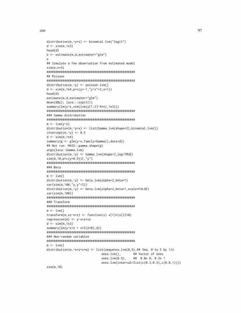
sim 97

distribution(m,~y+z) <- binomial.lvm("logit")d <- sim(m,1e3)head(d)e <- estimate(m,d,estimator="glm")e## Simulate a few observation from estimated modelsim(e,n=5)#################################################### Poisson##################################################distribution(m,~y) <- poisson.lvm()d <- sim(m,1e4,p=c(y=-1,"y~x"=2,z=1))head(d)estimate(m,d,estimator="glm")mean(d$z); lava:::expit(1)summary(lm(y~x,sim(lvm(y[1:2]~4*x),1e3)))##################################################### Gamma distribution##################################################m <- lvm(y~x)distribution(m,~y+x) <- list(Gamma.lvm(shape=2),binomial.lvm())intercept(m,~y) <- 0.5d <- sim(m,1e4)summary(g <- glm(y~x,family=Gamma(),data=d))## Not run: MASS::gamma.shape(g)args(lava::Gamma.lvm)distribution(m,~y) <- Gamma.lvm(shape=2,log=TRUE)sim(m,10,p=c(y=0.5))[,"y"]##################################################### Beta##################################################m <- lvm()distribution(m,~y) <- beta.lvm(alpha=2,beta=1)var(sim(m,100,"y,y"=2))distribution(m,~y) <- beta.lvm(alpha=2,beta=1,scale=FALSE)var(sim(m,100))##################################################### Transform##################################################m <- lvm()transform(m,xz~x+z) <- function(x) x[1]*(x[2]>0)regression(m) <- y~x+z+xzd <- sim(m,1e3)summary(lm(y~x+z + x*I(z>0),d))##################################################### Non-random variables##################################################m <- lvm()distribution(m,~x+z+v+w) <- list(sequence.lvm(0,5),## Seq. 0 to 5 by 1/n

ones.lvm(), ## Vector of onesones.lvm(0.5), ## 0.8n 0, 0.2n 1ones.lvm(interval=list(c(0.3,0.5),c(0.8,1))))

sim(m,10)

98 sim

##################################################### Cox model### piecewise constant hazard################################################m <- lvm(t~x)rates <- c(1,0.5); cuts <- c(0,5)## Constant rate: 1 in [0,5), 0.5 in [5,Inf)distribution(m,~t) <- coxExponential.lvm(rate=rates,timecut=cuts)## Not run:

d <- sim(m,2e4,p=c("t~x"=0.1)); d$status <- TRUEplot(timereg::aalen(survival::Surv(t,status)~x,data=d,

resample.iid=0,robust=0),spec=1)L <- approxfun(c(cuts,max(d$t)),f=1,

cumsum(c(0,rates*diff(c(cuts,max(d$t))))),method="linear")

curve(L,0,100,add=TRUE,col="blue")

## End(Not run)##################################################### Cox model### piecewise constant hazard, gamma frailty##################################################m <- lvm(y~x+z)rates <- c(0.3,0.5); cuts <- c(0,5)distribution(m,~y+z) <- list(coxExponential.lvm(rate=rates,timecut=cuts),

loggamma.lvm(rate=1,shape=1))## Not run:

d <- sim(m,2e4,p=c("y~x"=0,"y~z"=0)); d$status <- TRUEplot(timereg::aalen(survival::Surv(y,status)~x,data=d,

resample.iid=0,robust=0),spec=1)L <- approxfun(c(cuts,max(d$y)),f=1,

cumsum(c(0,rates*diff(c(cuts,max(d$y))))),method="linear")

curve(L,0,100,add=TRUE,col="blue")

## End(Not run)## Equivalent via transform (here with Aalens additive hazard model)m <- lvm(y~x)distribution(m,~y) <- aalenExponential.lvm(rate=rates,timecut=cuts)distribution(m,~z) <- Gamma.lvm(rate=1,shape=1)transform(m,t~y+z) <- prodsim(m,10)## Shared frailtym <- lvm(c(t1,t2)~x+z)rates <- c(1,0.5); cuts <- c(0,5)distribution(m,~y) <- aalenExponential.lvm(rate=rates,timecut=cuts)distribution(m,~z) <- loggamma.lvm(rate=1,shape=1)## Not run:mets::fast.reshape(sim(m,100),varying="t")

## End(Not run)##################################################### General multivariate distributions

sim 99

#################################################### Not run:m <- lvm()distribution(m,~y1+y2,oratio=4) <- VGAM::rbiplackcopksmooth2(sim(m,1e4),rgl=FALSE,theta=-20,phi=25)m <- lvm()distribution(m,~z1+z2,"or1") <- VGAM::rbiplackcopdistribution(m,~y1+y2,"or2") <- VGAM::rbiplackcopsim(m,10,p=c(or1=0.1,or2=4))

## End(Not run)m <- lvm()distribution(m,~y1+y2+y3,TRUE) <- function(n,...) rmvn0(n,sigma=diag(3)+1)var(sim(m,100))## Syntax also useful for univariate generators, e.g.m <- lvm(y~x+z)distribution(m,~y,TRUE) <- function(n) rnorm(n,mean=1000)sim(m,5)distribution(m,~y,"m1",0) <- rnormsim(m,5)sim(m,5,p=c(m1=100))##################################################### Regression design in other parameters#################################################### Variance heterogeneitym <- lvm(y~x)distribution(m,~y) <- function(n,mean,x) rnorm(n,mean,exp(x)^.5)if (interactive()) plot(y~x,sim(m,1e3))## Alternaively, calculate the standard error directlyaddvar(m) <- ~sd ## If 'sd' should be part of the resulting data.frameconstrain(m,sd~x) <- function(x) exp(x)^.5distribution(m,~y) <- function(n,mean,sd) rnorm(n,mean,sd)if (interactive()) plot(y~x,sim(m,1e3))## Regression on variance parameterm <- lvm()regression(m) <- y~xregression(m) <- v~x##distribution(m,~v) <- 0 # No stochastic term## Alternative:## regression(m) <- v[NA:0]~xdistribution(m,~y) <- function(n,mean,v) rnorm(n,mean,exp(v)^.5)if (interactive()) plot(y~x,sim(m,1e3))## Regression on shape parameter in Weibull modelm <- lvm()regression(m) <- y ~ z+vregression(m) <- s ~ exp(0.6*x-0.5*z)distribution(m,~x+z) <- binomial.lvm()distribution(m,~cens) <- coxWeibull.lvm(scale=1)distribution(m,~y) <- coxWeibull.lvm(scale=0.1,shape=~s)eventTime(m) <- time ~ min(y=1,cens=0)if (interactive()) {

d <- sim(m,1e3)require(survival)

100 sim.default

(cc <- coxph(Surv(time,status)~v+strata(x,z),data=d))plot(survfit(cc) ,col=1:4,mark.time=FALSE)

}##################################################### Categorical predictor##################################################m <- lvm()## categorical(m,K=3) <- "v"categorical(m,labels=c("A","B","C")) <- "v"regression(m,additive=FALSE) <- y~v## Not run:plot(y~v,sim(m,1000,p=c("y~v:2"=3)))

## End(Not run)m <- lvm()categorical(m,labels=c("A","B","C"),p=c(0.5,0.3)) <- "v"regression(m,additive=FALSE,beta=c(0,2,-1)) <- y~v## equivalent to:## regression(m,y~v,additive=FALSE) <- c(0,2,-1)regression(m,additive=FALSE,beta=c(0,4,-1)) <- z~vtable(sim(m,1e4)$v)glm(y~v, data=sim(m,1e4))glm(y~v, data=sim(m,1e4,p=c("y~v:1"=3)))

transform(m,v2~v) <- function(x) x=='A'sim(m,10)

##################################################### Pre-calculate object##################################################m <- lvm(y~x)m2 <- sim(m,'y~x'=2)sim(m,10,'y~x'=2)sim(m2,10) ## Faster

sim.default Wrapper function for mclapply

Description

Wrapper function for mclapply

Usage

## Default S3 method:sim(x = NULL, R = 100, f = NULL, colnames = NULL,

messages = lava.options()$messages, mc.cores, blocksize = 2L * mc.cores,cl, type = 1L, seed = NULL, args = list(), iter = FALSE, ...)

sim.default 101

Arguments

x function or ’sim’ object

R Number of replications or data.frame with parameters

f Optional function (i.e., if x is a matrix)

colnames Optional column names

messages Messages

mc.cores Number of cores to use

blocksize Split computations in blocks

cl (optional) cluster to use for parallelization

type type=0 is an alias for messages=1,mc.cores=1,blocksize=R

seed (optional) Seed (needed with cl=TRUE)

args (optional) list of named arguments passed to (mc)mapply

iter If TRUE the iteration number is passed as first argument to (mc)mapply

... Additional arguments to (mc)mapply

See Also

summary.sim plot.sim print.sim

Examples

m <- lvm(y~x+e)distribution(m,~y) <- 0distribution(m,~x) <- uniform.lvm(a=-1.1,b=1.1)transform(m,e~x) <- function(x) (1*x^4)*rnorm(length(x),sd=1)

onerun <- function(iter=NULL,...,n=2e3,b0=1,idx=2) {d <- sim(m,n,p=c("y~x"=b0))l <- lm(y~x,d)res <- c(coef(summary(l))[idx,1:2],

confint(l)[idx,],estimate(l,only.coef=TRUE)[idx,2:4])

names(res) <- c("Estimate","Model.se","Model.lo","Model.hi","Sandwich.se","Sandwich.lo","Sandwich.hi")

res}val <- sim(onerun,R=10,b0=1,messages=0,mc.cores=1)val

val <- sim(val,R=40,b0=1,mc.cores=1) ## append resultssummary(val,estimate=c(1,1),confint=c(3,4,6,7),true=c(1,1))

summary(val,estimate=c(1,1),se=c(2,5),names=c("Model","Sandwich"))summary(val,estimate=c(1,1),se=c(2,5),true=c(1,1),names=c("Model","Sandwich"),confint=TRUE)

if (interactive()) {plot(val,estimate=1,c(2,5),true=1,names=c("Model","Sandwich"),polygon=FALSE)

102 spaghetti

plot(val,estimate=c(1,1),se=c(2,5),main=NULL,true=c(1,1),names=c("Model","Sandwich"),line.lwd=1,col=c("gray20","gray60"),rug=FALSE)

plot(val,estimate=c(1,1),se=c(2,5),true=c(1,1),names=c("Model","Sandwich"))

}

f <- function(a=1,b=1) {rep(a*b,5)

}R <- Expand(a=1:3,b=1:3)sim(f,R,type=0)sim(function(a,b) f(a,b), 3, args=c(a=5,b=5),type=0)sim(function(iter=1,a=5,b=5) iter*f(a,b), type=0, iter=TRUE, R=5)

spaghetti Spaghetti plot

Description

Spaghetti plot for longitudinal data

Usage

spaghetti(formula, data, id = "id", group = NULL, type = "o", lty = 1,pch = NA, col = 1:10, alpha = 0.3, lwd = 1, level = 0.95,trend.formula = formula, tau = NULL, trend.lty = 1, trend.join = TRUE,trend.delta = 0.2, trend = !is.null(tau), trend.col = col,trend.alpha = 0.2, trend.lwd = 3, trend.jitter = 0, legend = NULL,by = NULL, xlab = "Time", ylab = "", add = FALSE, ...)

Arguments

formula Formula (response ~ time)

data data.frame

id Id variable

group group variable

type Type (line ’l’, stair ’s’, ...)

lty Line type

pch Colour

col Colour

alpha transparency (0-1)

lwd Line width

level Confidence level

spaghetti 103

trend.formula Formula for trendline

tau Quantile to estimate (trend)

trend.lty Trend line type

trend.join Trend polygon

trend.delta Length of limit bars

trend Add trend line

trend.col Colour of trend line

trend.alpha Transparency

trend.lwd Trend line width

trend.jitter Jitter amount

legend Legend

by make separate plot for each level in ’by’ (formula, name of column, or vector)

xlab Label of X-axis

ylab Label of Y-axis

add Add to existing device

... Additional arguments to lower level arguments

Author(s)

Klaus K. Holst

Examples

if (interactive() & requireNamespace("mets")) {K <- 5y <- "y"%++%seq(K)m <- lvm()regression(m,y=y,x=~u) <- 1regression(m,y=y,x=~s) <- seq(K)-1regression(m,y=y,x=~x) <- "b"N <- 50d <- sim(m,N); d$z <- rbinom(N,1,0.5)dd <- mets::fast.reshape(d); dd$num <- dd$num+3spaghetti(y~num,dd,id="id",lty=1,col=Col(1,.4),

trend.formula=~factor(num),trend=TRUE,trend.col="darkblue")dd$num <- dd$num+rnorm(nrow(dd),sd=0.5) ## Unbalancespaghetti(y~num,dd,id="id",lty=1,col=Col(1,.4),

trend=TRUE,trend.col="darkblue")spaghetti(y~num,dd,id="id",lty=1,col=Col(1,.4),

trend.formula=~num+I(num^2),trend=TRUE,trend.col="darkblue")}

104 stack.estimate

stack.estimate Stack estimating equations

Description

Stack estimating equations (two-stage estimator)

Usage

## S3 method for class 'estimate'stack(x, model2, D1u, inv.D2u, propensity, dpropensity, U,keep1 = FALSE, propensity.arg, estimate.arg, na.action = na.pass, ...)

Arguments

x Model 1

model2 Model 2

D1u Derivative of score of model 2 w.r.t. parameter vector of model 1

inv.D2u Inverse of deri

propensity propensity score (vector or function)

dpropensity derivative of propensity score wrt parameters of model 1

U Optional score function (model 2) as function of all parameters

keep1 If FALSE only parameters of model 2 is returned

propensity.arg Arguments to propensity function

estimate.arg Arguments to ’estimate’

na.action Method for dealing with missing data in propensity score


Examples

m <- lvm(z0~x)Missing(m, z ~ z0) <- r~xdistribution(m,~x) <- binomial.lvm()p <- c(r=-1,'r~x'=0.5,'z0~x'=2)beta <- p[3]/2d <- sim(m,500,p=p)m1 <- estimate(r~x,data=d,family=binomial)d$w <- d$r/predict(m1,type="response")m2 <- estimate(z~1, weights=w, data=d)(e <- stack(m1,m2,propensity=TRUE))

startvalues 105

startvalues For internal use

Description

For internal use

Author(s)

Klaus K. Holst

subset.lvm Extract subset of latent variable model

Description

Extract measurement models or user-specified subset of model

Usage

## S3 method for class 'lvm'subset(x, vars, ...)

Arguments

x lvm-object.

vars Character vector or formula specifying variables to include in subset.


Value

A lvm-object.

Author(s)

Klaus K. Holst

Examples

m <- lvm(c(y1,y2)~x1+x2)subset(m,~y1+x1)

106 timedep

summary.sim Summary method for ’sim’ objects

Description

Summary method for ’sim’ objects

Usage

## S3 method for class 'sim'summary(object, estimate = NULL, se = NULL,confint = !is.null(se) && !is.null(true), true = NULL, fun,names = NULL, unique.names = TRUE, minimal = FALSE, level = 0.95,quantiles = c(0.025, 0.5, 0.975), ...)

Arguments

object sim object

estimate (optional) columns with estimates

se (optional) columns with standard error estimates

confint (optional) list of pairs of columns with confidence limits

true (optional) vector of true parameter values

fun (optional) summary function

names (optional) names of

unique.names if TRUE, unique.names will be applied to column names

minimal if TRUE, minimal summary will be returned

level confidence level

quantiles quantiles

... additional levels to lower-level functions

timedep Time-dependent parameters

Description

Add time-varying covariate effects to model

Usage

timedep(object, formula, rate, timecut, type = "coxExponential.lvm", ...)

timedep 107

Arguments

object Model

formula Formula with rhs specifying time-varying covariates

rate Optional rate parameters. If given as a vector this parameter is interpreted as theraw (baseline-)rates within each time interval defined by timecut. If given asa matrix the parameters are interpreted as log-rates (and log-rate-ratios for thetime-varying covariates defined in the formula).

timecut Time intervals

type Type of model (default piecewise constant intensity)


Author(s)

Klaus K. Holst

Examples

## Piecewise constant hazardm <- lvm(y~1)m <- timedep(m,y~1,timecut=c(0,5),rate=c(0.5,0.3))

## Not run:d <- sim(m,1e4); d$status <- TRUEdd <- mets::lifetable(Surv(y,status)~1,data=d,breaks=c(0,5,10));exp(coef(glm(events ~ offset(log(atrisk)) + -1 + interval, dd, family=poisson)))

## End(Not run)

## Piecewise constant hazard and time-varying effect of z1m <- lvm(y~1)distribution(m,~z1) <- ones.lvm(0.5)R <- log(cbind(c(0.2,0.7,0.9),c(0.5,0.3,0.3)))m <- timedep(m,y~z1,timecut=c(0,3,5),rate=R)

## Not run:d <- sim(m,1e4); d$status <- TRUEdd <- mets::lifetable(Surv(y,status)~z1,data=d,breaks=c(0,3,5,Inf));exp(coef(glm(events ~ offset(log(atrisk)) + -1 + interval+z1:interval, dd, family=poisson)))

## End(Not run)

## Explicit simulation of time-varying effectsm <- lvm(y~1)distribution(m,~z1) <- ones.lvm(0.5)distribution(m,~z2) <- binomial.lvm(p=0.5)#variance(m,~m1+m2) <- 0

108 toformula

#regression(m,m1[m1:0] ~ z1) <- log(0.5)#regression(m,m2[m2:0] ~ z1) <- log(0.3)regression(m,m1 ~ z1,variance=0) <- log(0.5)regression(m,m2 ~ z1,variance=0) <- log(0.3)intercept(m,~m1+m2) <- c(-0.5,0)m <- timedep(m,y~m1+m2,timecut=c(0,5))

## Not run:d <- sim(m,1e5); d$status <- TRUEdd <- mets::lifetable(Surv(y,status)~z1,data=d,breaks=c(0,5,Inf))exp(coef(glm(events ~ offset(log(atrisk)) + -1 + interval + interval:z1, dd, family=poisson)))

## End(Not run)

toformula Converts strings to formula

Description

Converts a vector of predictors and a vector of responses (characters) i#nto a formula expression.

Usage

toformula(y = ".", x = ".")

Arguments

y vector of predictors

x vector of responses

Value

An object of class formula

Author(s)

Klaus K. Holst

See Also

as.formula,

Examples

toformula(c("age","gender"), "weight")

tr 109

tr Trace operator

Description

Calculates the trace of a square matrix.

Usage

tr(x, ...)

Arguments

x Square numeric matrix


Value

numeric

Author(s)

Klaus K. Holst

See Also

crossprod, tcrossprod

Examples

tr(diag(1:5))

trim Trim tring of (leading/trailing/all) white spaces

Description

Trim tring of (leading/trailing/all) white spaces

Usage

trim(x, all = FALSE, ...)

110 twostage

Arguments

x String

all Trim all whitespaces?


Author(s)

Klaus K. Holst

twindata Twin menarche data

Description

Simulated data

id numeric Twin-pair idzyg character Zygosity (MZ or DZ)

twinnum numeric Twin number (1 or 2)agemena numeric Age at menarche (or censoring)

status logical Censoring status (observed:=T,censored:=F)bw numeric Birth weight

msmoke numeric Did mother smoke? (yes:=1,no:=0)

Format

data.frame

Source

Simulated

twostage Two-stage estimator

Description

Generic function.

Usage

twostage(object, ...)

twostage.lvmfit 111

Arguments

object Model object


See Also

twostage.lvm twostage.lvmfit twostage.lvm.mixture twostage.estimate

twostage.lvmfit Two-stage estimator (non-linear SEM)

Description

Two-stage estimator for non-linear structural equation models

Usage

## S3 method for class 'lvmfit'twostage(object, model2, data = NULL, predict.fun = NULL,id1 = NULL, id2 = NULL, all = FALSE, formula = NULL, std.err = TRUE,...)

Arguments

object Stage 1 measurement model

model2 Stage 2 SEM

data data.frame

predict.fun Prediction of latent variable

id1 Optional id-variable (stage 1 model)

id2 Optional id-variable (stage 2 model)

all If TRUE return additional output (naive estimates)

formula optional formula specifying non-linear relation

std.err If FALSE calculations of standard errors will be skipped


Examples

m <- lvm(c(x1,x2,x3)~f1,f1~z,c(y1,y2,y3)~f2,f2~f1+z)

latent(m) <- ~f1+f2d <- simulate(m,100,p=c("f2,f2"=2,"f1,f1"=0.5),seed=1)

## Full MLEee <- estimate(m,d)

112 twostage.lvmfit

## Manual two-stage## Not run:m1 <- lvm(c(x1,x2,x3)~f1,f1~z); latent(m1) <- ~f1e1 <- estimate(m1,d)pp1 <- predict(e1,f1~x1+x2+x3)

d$u1 <- pp1[,]d$u2 <- pp1[,]^2+attr(pp1,"cond.var")[1]m2 <- lvm(c(y1,y2,y3)~eta,c(y1,eta)~u1+u2+z); latent(m2) <- ~etae2 <- estimate(m2,d)

## End(Not run)

## Two-stagem1 <- lvm(c(x1,x2,x3)~f1,f1~z); latent(m1) <- ~f1m2 <- lvm(c(y1,y2,y3)~eta,c(y1,eta)~u1+u2+z); latent(m2) <- ~etapred <- function(mu,var,data,...)

cbind("u1"=mu[,1],"u2"=mu[,1]^2+var[1])(mm <- twostage(m1,model2=m2,data=d,predict.fun=pred))

if (interactive()) {pf <- function(p) p["eta"]+p["eta~u1"]*u + p["eta~u2"]*u^2plot(mm,f=pf,data=data.frame(u=seq(-2,2,length.out=100)),lwd=2)

}

## Splinesf <- function(x) cos(2*x)+x+-0.25*x^2m <- lvm(x1+x2+x3~eta1, y1+y2+y3~eta2, latent=~eta1+eta2)functional(m, eta2~eta1) <- fd <- sim(m,500,seed=1,latent=TRUE)m1 <- lvm(x1+x2+x3~eta1,latent=~eta1)m2 <- lvm(y1+y2+y3~eta2,latent=~eta2)mm <- twostage(m1,m2,formula=eta2~eta1,type="spline")if (interactive()) plot(mm)

nonlinear(m2,type="quadratic") <- eta2~eta1a <- twostage(m1,m2,data=d)if (interactive()) plot(a)

kn <- c(-1,0,1)nonlinear(m2,type="spline",knots=kn) <- eta2~eta1a <- twostage(m1,m2,data=d)x <- seq(-3,3,by=0.1)y <- predict(a, newdata=data.frame(eta1=x))

if (interactive()) {plot(eta2~eta1, data=d)lines(x,y, col="red", lwd=5)

p <- estimate(a,f=function(p) predict(a,p=p,newdata=x))$coefmatplot(eta2~eta1, data=d)lines(x,p[,1], col="red", lwd=5)confband(x,lower=p[,3],upper=p[,4],center=p[,1], polygon=TRUE, col=Col(2,0.2))

twostageCV 113

l1 <- lm(eta2~splines::ns(eta1,knots=kn),data=d)p1 <- predict(l1,newdata=data.frame(eta1=x),interval="confidence")lines(x,p1[,1],col="green",lwd=5)confband(x,lower=p1[,2],upper=p1[,3],center=p1[,1], polygon=TRUE, col=Col(3,0.2))

}

## Not run: ## Reduce timing## Cross-validation examplema <- lvm(c(x1,x2,x3)~u,latent=~u)ms <- functional(ma, y~u, f=function(x) -.4*x^2)d <- sim(ms,500)#,seed=1)ea <- estimate(ma,d)

mb <- lvm()mb1 <- nonlinear(mb,type="linear",y~u)mb2 <- nonlinear(mb,type="quadratic",y~u)mb3 <- nonlinear(mb,type="spline",knots=c(-3,-1,0,1,3),y~u)mb4 <- nonlinear(mb,type="spline",knots=c(-3,-2,-1,0,1,2,3),y~u)ff <- lapply(list(mb1,mb2,mb3,mb4),

function(m) function(data,...) twostage(ma,m,data=data,st.derr=FALSE))a <- cv(ff,data=d,rep=1,mc.cores=1)a

## End(Not run)

twostageCV Cross-validated two-stage estimator

Description

Cross-validated two-stage estimator for non-linear SEM

Usage

twostageCV(model1, model2, data, control1 = list(trace = 0),control2 = list(trace = 0), knots.boundary, mc.cores = 1, k = 1:4,nknots = 1:9, fix = TRUE, std.err = TRUE, nfolds = 5, rep = 1, ...)

Arguments

model1 model 1 (exposure measurement error model)

model2 model 2

data data.frame

control1 optimization parameters for model 1

control2 optimization parameters for model 1

knots.boundary boundary points for natural cubic spline basis

114 vars

mc.cores number of cores to use for parallel computations

k number of mixture components

nknots number of knots

fix automatically fix parameters for identification (TRUE)

std.err calculation of standard errors (TRUE)

nfolds Number of folds (cross-validation)

rep Number of repeats of cross-validation


Examples

## Not run: ## Reduce Ex.Timingsm1 <- lvm( x1+x2+x3 ~ u1, latent= ~u1)m2 <- lvm( y1+y2+y3 ~ u2, latent= ~u2)m <- functional(merge(m1,m2), u2~u1, f=function(x) sin(x)+x)n <- 200distribution(m, ~u1) <- uniform.lvm(-6,6)d <- sim(m,n=200,seed=1)val <- twostageCV(m1,m2,data=d, std.err=FALSE, nknots=2:5, K=1:3, mc.cores=1, nfolds=5)

## End(Not run)

vars Extract variable names from latent variable model

Description

Extract exogenous variables (predictors), endogenous variables (outcomes), latent variables (ran-dom effects), manifest (observed) variables from a lvm object.

Usage

vars(x,...)

endogenous(x,...)

exogenous(x,...)

manifest(x,...)

latent(x,...)

## S3 replacement method for class 'lvm'exogenous(x, xfree = TRUE,...) <- value

## S3 method for class 'lvm'

vars 115

exogenous(x,latent=FALSE,index=TRUE,...)

## S3 replacement method for class 'lvm'latent(x,clear=FALSE,...) <- value

Arguments

x lvm-object


latent Logical defining whether latent variables without parents should be included inthe result

index For internal use only

clear Logical indicating whether to add or remove latent variable status

xfree For internal use only

value Formula or character vector of variable names.

Details

vars returns all variables of the lvm-object including manifest and latent variables. Similarilymanifest and latent returns the observered resp. latent variables of the model. exogenous re-turns all manifest variables without parents, e.g. covariates in the model, however the argumentlatent=TRUE can be used to also include latent variables without parents in the result. Pr. defaultlava will not include the parameters of the exogenous variables in the optimisation routine duringestimation (likelihood of the remaining observered variables conditional on the covariates), how-ever this behaviour can be altered via the assignment function exogenous<- telling lava whichsubset of (valid) variables to condition on. Finally latent returns a vector with the names of thelatent variables in x. The assigment function latent<- can be used to change the latent status ofvariables in the model.

Value

Vector of variable names.

Author(s)

Klaus K. Holst

See Also

endogenous, manifest, latent, exogenous, vars

Examples

g <- lvm(eta1 ~ x1+x2)regression(g) <- c(y1,y2,y3) ~ eta1latent(g) <- ~eta1endogenous(g)

116 wait

exogenous(g)identical(latent(g), setdiff(vars(g),manifest(g)))

vec vec operator

Description

vec operator

Usage

vec(x, matrix = FALSE, sep = ".", ...)

Arguments

x Array

matrix If TRUE a row vector (matrix) is returned

sep Seperator


Details

Convert array into vector

Author(s)

Klaus Holst

wait Wait for user input (keyboard or mouse)

Description

Wait for user input (keyboard or mouse)

Usage

wait()

Author(s)

Klaus K. Holst

wrapvec 117

wrapvec Wrap vector

Description

Wrap vector

Usage

wrapvec(x, delta = 0L, ...)

Arguments

x Vector or integer

delta Shift

... Additional parameters

Examples

wrapvec(5,2)

zibreg Regression model for binomial data with unkown group of immortals

Description

Regression model for binomial data with unkown group of immortals (zero-inflated binomial re-gression)

Usage

zibreg(formula, formula.p = ~1, data, family = stats::binomial(),offset = NULL, start, var = "hessian", ...)

Arguments

formula Formula specifying

formula.p Formula for model of disease prevalence

data data frame

family Distribution family (see the help page family)

offset Optional offset

start Optional starting values

var Type of variance (robust, expected, hessian, outer)


118 %++%

Author(s)

Klaus K. Holst

Examples

## Simulationn <- 2e3x <- runif(n,0,20)age <- runif(n,10,30)z0 <- rnorm(n,mean=-1+0.05*age)z <- cut(z0,breaks=c(-Inf,-1,0,1,Inf))p0 <- lava:::expit(model.matrix(~z+age) %*% c(-.4, -.4, 0.2, 2, -0.05))y <- (runif(n)<lava:::tigol(-1+0.25*x-0*age))*1u <- runif(n)<p0y[u==0] <- 0d <- data.frame(y=y,x=x,u=u*1,z=z,age=age)head(d)

## Estimatione0 <- zibreg(y~x*z,~1+z+age,data=d)e <- zibreg(y~x,~1+z+age,data=d)compare(e,e0)ePD(e0,intercept=c(1,3),slope=c(2,6))

B <- rbind(c(1,0,0,0,20),c(1,1,0,0,20),c(1,0,1,0,20),c(1,0,0,1,20))

prev <- summary(e,pr.contrast=B)$prevalence

x <- seq(0,100,length.out=100)newdata <- expand.grid(x=x,age=20,z=levels(d$z))fit <- predict(e,newdata=newdata)plot(0,0,type="n",xlim=c(0,101),ylim=c(0,1),xlab="x",ylab="Probability(Event)")count <- 0for (i in levels(newdata$z)) {

count <- count+1lines(x,fit[which(newdata$z==i)],col="darkblue",lty=count)

}abline(h=prev[3:4,1],lty=3:4,col="gray")abline(h=prev[3:4,2],lty=3:4,col="lightgray")abline(h=prev[3:4,3],lty=3:4,col="lightgray")legend("topleft",levels(d$z),col="darkblue",lty=seq_len(length(levels(d$z))))

%++% Concatenation operator

%ni% 119

Description

For matrices a block-diagonal matrix is created. For all other data types he operator is a wrapper ofpaste.

Usage

x %++% y

Arguments

x First object

y Second object of same class

Details

Concatenation operator

Author(s)

Klaus K. Holst

See Also

blockdiag, paste, cat,

Examples

## Block diagonalmatrix(rnorm(25),5)%++%matrix(rnorm(25),5)## String concatenation"Hello "%++%" World"## Function compositionf <- log %++% expf(2)

%ni% Matching operator (x not in y) oposed to the %in%-operator (x in y)

Description

Matching operator

Usage

x %ni% y

120 %ni%

Arguments

x vector

y vector of same type as x

Value

A logical vector.

Author(s)

Klaus K. Holst

See Also

match

Examples

1:10 %ni% c(1,5,10)

Index

∗Topic algebratr, 109

∗Topic aplotlabels<-, 57

∗Topic colorCol, 14

∗Topic datagensim, 96

∗Topic datasetsbmd, 7bmidata, 7brisa, 9calcium, 11hubble, 51hubble2, 51indoorenv, 54missingdata, 64nldata, 71nsem, 72semdata, 94serotonin, 94serotonin2, 95twindata, 110

∗Topic graphsGraph, 49labels<-, 57path, 76

∗Topic hplot,plotConf, 84

∗Topic hplotdevcoords, 33plot.lvm, 80rotate2, 93

∗Topic htestcompare, 17modelsearch, 67

∗Topic iplotclick, 12confband, 19

pdfconvert, 78wait, 116

∗Topic manipNA2x, 71

∗Topic mathtr, 109

∗Topic methodsgof, 47path, 76

∗Topic misc%++%, 118%ni%, 119Grep, 50

∗Topic models,mixture, 65mvnmix, 69

∗Topic modelsbootstrap.lvm, 8complik, 18confint.lvmfit, 21constrain<-, 23covariance, 28estimate.lvm, 39eventTime, 42gof, 47Graph, 49intercept, 54lava.options, 59lvm, 60Model, 66partialcor, 75path, 76regression<-, 89rmvar, 92sim, 96subset.lvm, 105toformula, 108vars, 114

∗Topic package

121

122 INDEX

lava-package, 4∗Topic regression

bootstrap.lvm, 8complik, 18confint.lvmfit, 21constrain<-, 23covariance, 28estimate.lvm, 39eventTime, 42intercept, 54lvm, 60mixture, 65mvnmix, 69partialcor, 75plot.lvm, 80plotConf, 84regression<-, 89rmvar, 92sim, 96subset.lvm, 105vars, 114

∗Topic survivaleventTime, 42

∗Topic utilities%++%, 118%ni%, 119Grep, 50makemissing, 61startvalues, 105toformula, 108

%++%, 118%ni%, 119

aalenExponential.lvm (sim), 96addattr (startvalues), 105addhook (startvalues), 105addvar, 5addvar<- (addvar), 5adjMat (children), 12agrep, 51ancestors (children), 12as.formula, 108as.sim (sim.default), 100

backdoor, 5baptize, 6beta.lvm (sim), 96binomial.lvm (sim), 96blockdiag, 6

bmd, 7bmidata, 7bootstrap, 7, 22bootstrap.lvm, 8bootstrap.lvmfit (bootstrap.lvm), 8brisa, 9By, 10

calcium, 11cancel, 11cancel<- (cancel), 11cat, 119categorical (sim), 96categorical<- (sim), 96checkmultigroup (startvalues), 105children, 12chisq.lvm (sim), 96click, 12closed.testing, 13CoefMat (startvalues), 105Col, 14colorbar, 15colsel (click), 12Combine, 16commutation, 17compare, 17, 35, 68complik, 18confband, 19confint.lvmfit, 9, 21confint.multigroupfit (confint.lvmfit),

21confpred, 22constrain (constrain<-), 23constrain<-, 23constraints (constrain<-), 23contr, 27correlation, 27covariance, 25, 28, 60covariance<- (covariance), 28covfix (covariance), 28covfix<- (covariance), 28coxExponential.lvm (sim), 96coxGompertz.lvm (sim), 96coxWeibull.lvm (sim), 96crossprod, 109csplit, 30curly, 31cv, 32

INDEX 123

decomp.specials (startvalues), 105density.sim (plot.sim), 82deriv (startvalues), 105descendants (children), 12describecoef (startvalues), 105devcoords, 33diagtest, 33Diff (diagtest), 33distribution (sim), 96distribution<- (sim), 96dmvn0 (startvalues), 105dsep (dsep.lvm), 34dsep.lvm, 34

edgelabels (labels<-), 57edgelabels<- (labels<-), 57edgeList (children), 12effects (path), 76endogenous, 115endogenous (vars), 114equivalence, 18, 35, 68estimate (estimate.default), 36estimate.default, 36estimate.lvm, 39estimate.MAR (startvalues), 105eventTime, 42eventTime<- (eventTime), 42exogenous, 115exogenous (vars), 114exogenous<- (vars), 114Expand, 45expit (startvalues), 105

finalize (startvalues), 105fixsome (startvalues), 105foldr (csplit), 30forestplot (confband), 19fplot, 45functional (sim), 96functional<- (sim), 96

Gamma.lvm (sim), 96gamma.lvm (sim), 96gaussian.lvm (sim), 96gaussian_logLik.lvm (startvalues), 105gethook (startvalues), 105getMplus, 46getoutcome (startvalues), 105getSAS, 47

gkgamma (multinomial), 68GM2.lvm (sim), 96GM3.lvm (sim), 96gof, 47Graph, 49, 67graph2lvm (startvalues), 105Graph<- (Graph), 49Grep, 50grep, 51

heavytail (sim), 96heavytail<- (sim), 96hubble, 51hubble2, 51

idplot, 13idplot (click), 12igraph.lvm (startvalues), 105iid, 52images, 52index (startvalues), 105index<- (startvalues), 105indoorenv, 54information (gof), 47intercept, 25, 54, 60intercept<- (intercept), 54intfix (intercept), 54intfix<- (intercept), 54Inverse (startvalues), 105IV (startvalues), 105

kappa.multinomial (multinomial), 68kappa.table (multinomial), 68kill (rmvar), 92kill<- (rmvar), 92km, 56ksmooth2, 56

labels (labels<-), 57labels<-, 57latent, 115latent (vars), 114latent<- (vars), 114lava (lava-package), 4lava-package, 4lava.options, 59lisrel (startvalues), 105loggamma.lvm (sim), 96logit (startvalues), 105

124 INDEX

logit.lvm (sim), 96logLik.lvmfit (gof), 47lognormal.lvm (sim), 96lvm, 60

makemissing, 61manifest, 115manifest (vars), 114match, 120matrices (startvalues), 105measurement (subset.lvm), 105measurement.error, 61merge (startvalues), 105merge.estimate (estimate.default), 36Missing, 63Missing, (Missing), 63Missing<- (Missing), 63missingdata, 64missingModel (startvalues), 105mixture, 65Model, 50, 66Model<- (Model), 66modelPar (startvalues), 105modelsearch, 18, 35, 67modelVar (startvalues), 105moments (gof), 47multigroup (startvalues), 105multinomial, 68mvn.lvm (sim), 96mvnmix, 69

na.pass0 (startvalues), 105NA2x, 71nldata, 71nodecolor (labels<-), 57nodecolor<- (labels<-), 57nonlinear (twostage.lvmfit), 111nonlinear<- (twostage.lvmfit), 111normal.lvm (sim), 96NR (startvalues), 105nsem, 72

odds (diagtest), 33offdiag (revdiag), 91offdiag<- (revdiag), 91offdiags (startvalues), 105ones.lvm (sim), 96OR (diagtest), 33ordinal (ordinal<-), 72

ordinal<-, 72ordreg, 73Org, 73

p.correct (closed.testing), 13parameter (startvalues), 105parameter<- (constrain<-), 23parents (children), 12pareto.lvm (sim), 96parfix (startvalues), 105parfix<- (startvalues), 105parlabels (startvalues), 105parpos, 74pars (startvalues), 105parsedesign (contr), 27partialcor, 75paste, 119path, 76pcor, 77PD, 78pdfconvert, 78plot.estimate, 79plot.lvm, 80plot.lvmfit (plot.lvm), 80plot.sim, 82plotConf, 84poisson.lvm (sim), 96predict.lvm, 86predict.lvmfit (predict.lvm), 86predictlvm, 87print.lvm (lvm), 60probit.lvm (sim), 96procdata.lvmfit (startvalues), 105procformula (startvalues), 105profci (startvalues), 105

randomslope (startvalues), 105randomslope<- (startvalues), 105Range.lvm, 88Ratio (diagtest), 33regfix (regression<-), 89regfix<- (regression<-), 89regression, 25, 60regression (regression<-), 89regression<-, 89reindex (startvalues), 105reorderdata (startvalues), 105revdiag, 91revdiag<- (revdiag), 91

INDEX 125

riskcomp (diagtest), 33rmvar, 92rmvar<- (rmvar), 92rmvn0 (startvalues), 105roots (children), 12rot2D (rotate2), 93rot3D (rotate2), 93rotate2, 93rsq (startvalues), 105

scheffe, 93score (gof), 47score.glm (startvalues), 105semdata, 94sequence.lvm (sim), 96serotonin, 94serotonin2, 95sim, 96sim.default, 100simulate.lvm (sim), 96simulate.lvmfit (sim), 96sinks (children), 12spaghetti, 102Specials (startvalues), 105stack.estimate, 104starter.multigroup (startvalues), 105startvalues, 105startvalues0 (startvalues), 105startvalues1 (startvalues), 105startvalues2 (startvalues), 105startvalues3 (startvalues), 105stdcoef (startvalues), 105student.lvm (sim), 96subgraph (startvalues), 105subset.lvm, 105summary.lvm (lvm), 60summary.sim, 106surface (ksmooth2), 56

tcrossprod, 109threshold.lvm (sim), 96tigol (startvalues), 105timedep, 106timedep<- (timedep), 106toformula, 108totaleffects (path), 76tr, 109transform.lvm (sim), 96transform<- (sim), 96

trim, 109twindata, 110twostage, 110twostage.estimate (twostage.lvmfit), 111twostage.lvm (twostage.lvmfit), 111twostage.lvmfit, 111twostageCV, 113

uniform.lvm (sim), 96updatelvm (startvalues), 105

variance (covariance), 28variance<- (covariance), 28variances (startvalues), 105vars, 114, 115vec, 116

wait, 116waitclick (wait), 116weibull.lvm (sim), 96Weights (startvalues), 105wrapvec, 117

x2NA (NA2x), 71

zibreg, 117

Documents

Package ‘lava’ - The Comprehensive R Archive Network 5 addvar Add variable to (model) object Description Generic method for adding variables to model object Usage addvar(x, ...)