Package ‘LIM’ - The Comprehensive R Archive Network lim ... (package="LIM"), "/doc/examples/Foodweb ... Mathematically this can be estimated by solving a linear programming problem:

Package ‘LIM’February 19, 2015

Version 1.4.6

Title Linear Inverse Model examples and solution methods.

Author Karline Soetaert <[email protected]>,Dick van Oevelen<[email protected]>

Maintainer Karline Soetaert <[email protected]>

Depends R (>= 2.10), limSolve, diagram

Description Functions that read and solve linear inverse problems (food web problems, linear pro-gramming problems).These problems find solutions to linear or quadratic functions:min or max (f(x)), where f(x) = ||Ax-b||^2 or f(x) = sum(ai*xi)subject to equality constraints Ex=f and inequality constraints Gx>=h. Uses package limSolve.

License GPL (>= 2)

LazyData yes

Repository CRAN

Repository/R-Forge/Project lim

Repository/R-Forge/Revision 57

Repository/R-Forge/DateTimeStamp 2014-12-24 13:23:18

Date/Publication 2014-12-26 11:07:11

NeedsCompilation no

R topics documented:LIM-package . . . . . . . . . . . . . . . . . . . . . . . . . . . . . . . . . . . . . . . . 2FILERigaAutumn . . . . . . . . . . . . . . . . . . . . . . . . . . . . . . . . . . . . . . 4Flowmatrix . . . . . . . . . . . . . . . . . . . . . . . . . . . . . . . . . . . . . . . . . 5Ldei . . . . . . . . . . . . . . . . . . . . . . . . . . . . . . . . . . . . . . . . . . . . . 6LIMBlending . . . . . . . . . . . . . . . . . . . . . . . . . . . . . . . . . . . . . . . . 8LIMBrouageMudflat . . . . . . . . . . . . . . . . . . . . . . . . . . . . . . . . . . . . 10LIMCaliforniaSediment . . . . . . . . . . . . . . . . . . . . . . . . . . . . . . . . . . . 11LIMCoralRockall . . . . . . . . . . . . . . . . . . . . . . . . . . . . . . . . . . . . . . 13LIMEcoli . . . . . . . . . . . . . . . . . . . . . . . . . . . . . . . . . . . . . . . . . . 14

1

2 LIM-package

LIMEverglades . . . . . . . . . . . . . . . . . . . . . . . . . . . . . . . . . . . . . . . 16LIMRigaAutumn . . . . . . . . . . . . . . . . . . . . . . . . . . . . . . . . . . . . . . 18LIMRigaSpring . . . . . . . . . . . . . . . . . . . . . . . . . . . . . . . . . . . . . . . 19LIMRigaSummer . . . . . . . . . . . . . . . . . . . . . . . . . . . . . . . . . . . . . . 20LIMScheldtIntertidal . . . . . . . . . . . . . . . . . . . . . . . . . . . . . . . . . . . . 21LIMTakapoto . . . . . . . . . . . . . . . . . . . . . . . . . . . . . . . . . . . . . . . . 23Linp . . . . . . . . . . . . . . . . . . . . . . . . . . . . . . . . . . . . . . . . . . . . . 24Lsei . . . . . . . . . . . . . . . . . . . . . . . . . . . . . . . . . . . . . . . . . . . . . 26Plotranges . . . . . . . . . . . . . . . . . . . . . . . . . . . . . . . . . . . . . . . . . . 28PrintMat . . . . . . . . . . . . . . . . . . . . . . . . . . . . . . . . . . . . . . . . . . . 30Read . . . . . . . . . . . . . . . . . . . . . . . . . . . . . . . . . . . . . . . . . . . . . 31Setup . . . . . . . . . . . . . . . . . . . . . . . . . . . . . . . . . . . . . . . . . . . . 33Variables . . . . . . . . . . . . . . . . . . . . . . . . . . . . . . . . . . . . . . . . . . 35Varranges . . . . . . . . . . . . . . . . . . . . . . . . . . . . . . . . . . . . . . . . . . 36Xranges . . . . . . . . . . . . . . . . . . . . . . . . . . . . . . . . . . . . . . . . . . . 37Xsample . . . . . . . . . . . . . . . . . . . . . . . . . . . . . . . . . . . . . . . . . . . 38

Index 40

LIM-package Linear Inverse Model examples and solution methods

Description

functions that read and solve linear inverse problems (food web problems, linear programmingproblems, flux balance analysis).

These problems find solutions to linear or quadratic functions: min or max (f(x)), where f(x) =||Ax− b||2 or f(x) = sum(ai ∗ xi)subject to equality constraints Ex = f and inequality constraints Gx >= h.

Uses package limSolve.

Details

Package: LIMType: PackageVersion: 1.4.3Date: 2011-09-05License: GNU Public License 2 or above

The model problem is formulated in text files in a way that is natural and comprehensible. Functionsin LIM then converts this input into the required linear equality and inequality conditions, which canbe solved either by least squares or by linear programming techniques. By letting an algorithmformulate the mathematics, it is simple to reformulate the model in case a parameter value changes,or a component is added or removed.

Three different types of problems are supported:

LIM-package 3

flow networks,

reaction networks (e.g. flux balance analysis).

and other (operations research) problems.

The first two cases are based on mass balances of the components.

The package includes many examples

Author(s)

Karline Soetaert (Maintainer),

Dick van Oevelen

References

Description of the software:

van Oevelen D, Van den Meersche K, Meysman FJR Soetaert K, Middelburg JJ, Vezina AF.,2009. Quantifying Food Web Flows Using Linear Inverse Models. Ecosystems 13: 32-45 DOI:10.1007/s10021-009-9297-6. http://www.springerlink.com/content/4q6h4011511731m5/fulltext.pdf

(please use the above citation when using the software)

About food web modelling:

Soetaert, K., van Oevelen, D., 2009. Modeling food web interactions in benthic deep-sea ecosys-tems: a practical guide. Oceanography (22) 1: 130-145.

Application of deep-water food web:

van Oevelen, Dick, Gerard Duineveld, Marc Lavaleye, Furu Mienis, Karline Soetaert, and Carlo H.R. Heip, 2009. The cold-water coral community as hotspot of carbon cycling on continental mar-gins: A food web analysis from Rockall Bank (northeast Atlantic). Limnology and Oceangraphy54:1829-1844.

http://www.aslo.org/lo/toc/vol_54/issue_6/1829.pdf

A flux balance analysis application:

Karline Soetaert. Escherichia coli Core Metabolism Model in LIM. LIM package vignette (see alsobelow).

See Also

Read, Setup for reading files and creating the model

Ldei, Lsei,Linp,

Flowmatrix, Plotranges, Variables,

Varranges, Xranges, Xsample.

http://www.springerlink.com/content/4q6h4011511731m5/fulltext.pdf

http://www.springerlink.com/content/4q6h4011511731m5/fulltext.pdf


4 FILERigaAutumn

Examples

## Not run:## show examples (see respective help pages for details)example(Lsei)example(LIMRigaSpring)example(Ldei)example(Xsample)example(Varranges)

## run demosdemo("LIMexamples")

## open the directory with R sourcecode examplesbrowseURL(paste(system.file(package="LIM"), "/doc/examples/Foodweb", sep=""))browseURL(paste(system.file(package="LIM"), "/doc/examples/LinearProg", sep=""))browseURL(paste(system.file(package="LIM"), "/doc/examples/Reactions", sep=""))

## the deep-water coral food -webbrowseURL(paste(system.file(package="LIM"), "/doc/examples/Foodweb/coral", sep=""))

## show package vignette with tutorial about how to create input filesvignette("LIM")

## E.coli example vignette - flux balance analysisvignette("LIMecoli")

browseURL(paste(system.file(package="LIM"), "/doc", sep=""))

## End(Not run)

FILERigaAutumn Input text "file" for gulf of Riga autumn planktonic food web

Description

Input text "file" for the Carbon flux Gulf of Riga planktonic food web in autumn as described inDonali et al. (1999).

The Gulf of Riga is a highly eutrophic system in the Baltic Sea

The foodweb comprises 7 functional compartments and two external compartments, connected with26 flows.

Units of the flows are mg C/m3/day

The "dataset" RigaAutumnFile is included to demonstrate the use of a text input file for food webmodels.

The original file, RigaAutumn.input can be found in subdirectory ‘web’ of the packages directory

In this subdirectory you will find many foodweb example input files

• They can be read using Read(file)• Or they can be directly solved using Setup(file)

Flowmatrix 5

Usage

data(FILERigaAutumn)

Format

vector of character strings as present in the original file

Author(s)

Karline Soetaert <[email protected]>

References

Donali, E., Olli, K., Heiskanen, A.S., Andersen, T., 1999. Carbon flow patterns in the planktonicfood web of the Gulf of Riga, the Baltic Sea: a reconstruction by the inverse method. Journal ofMarine Systems 23, 251..268.

See Also

LIMRigaAutumn a list containing the linear inverse model specification, generated from file ‘RigaAutumn.input’

Examples

print(FILERigaAutumn)

# RigaAutumnInput is a vector of text strings -# here it is first converted to a "File"# When using the example files in the LIM directory,# this first statement is not necessary## Not run:File <- textConnection(FILERigaAutumn)RigaAutumn.input <- Read(File)

## End(Not run)

Flowmatrix Generates a flow matrix for an inverse (foodweb) problem

Description

Given a linear inverse model food web input list, generates a flow matrix, that contains the valuesof flows

Usage

Flowmatrix(lim, web = NULL)

6 Ldei

Arguments

lim a list that contains the linear inverse model specification, as generated by func-tion setup.limfile.

web the solved (food) web problem, i.e. the values of the unknowns; if not specified,the model is solved first, using Ldei

Value

the flow matrix, containing the magnitude of the flows.

The value on row i and column j is the flow *from* i and *to* j

Author(s)


See Also

plotweb from package diagram, which takes as input the flow matrix and plots the food web

Examples

Flowmatrix(LIMRigaAutumn)

Ldei Solves a linear inverse model using least distance programming

Description

Solves a linear inverse model using least distance programming, i.e. minimizes the sum of squaredunknowns.

Input presented either:

• as matrices E, F, A, B, G, H (Ldei.double)

• as a list (Ldei.lim) or

• as a lim input file (Ldei.limfile)

Usage

Ldei(...)## S3 method for class 'lim'Ldei(lim, ...)## S3 method for class 'limfile'Ldei(file, verbose = TRUE, ...)## S3 method for class 'character'Ldei(...)## S3 method for class 'double'Ldei(...)

Ldei 7

Arguments


file name of the inverse input file.verbose if TRUE: prints warnings and messages to the screen.... other arguments passed to function ldei from packagelimSolve.

Details

Solves the following inverse problem:

min(∑

Costi ∗ xi2)

subject toAx = B

Gx >= H

Value

a list containing:

X vector containing the solution of the least distance problem.unconstrained.Solution

vector containing the unconstrained solution of the least distance problem.residualNorm scalar, the sum of residuals of equalities and violated inequalities.solutionNorm scalar, the value of the quadratic function at the solution.IsError logical, TRUE, if an error occurred.Error ldei error text.type ldei.

Author(s)


References

Lawson C.L.and Hanson R.J. 1974. SOLVING LEAST SQUARES PROBLEMS, Prentice-Hall

Lawson C.L.and Hanson R.J. 1995. Solving Least Squares Problems. SIAM classics in appliedmathematics, Philadelphia. (reprint of book)

See Also

ldei, the more general function from package limSolve.

Linp, to solve the linear inverse problem by linear programming.

Lsei, to solve the linear inverse problem by lsei (least squares with equality and inequality con-straints).

function ldei from packagelimSolve.

8 LIMBlending

Examples

Ldei(LIMRigaAutumn)

LIMBlending A blending problem specification

Description

A manufacturer produces a feeding mix for pet animals.

The feed mix contains two nutritive ingredients and one ingredient (filler) to provide bulk.

One kg of feed mix must contain a minimum quantity of each of four nutrients as below:

Nutrient A B C Dgram 80 50 25 5

The ingredients have the following nutrient values and cost

(gram/kg) A B C D Cost/kgIngredient 1 100 50 40 10 40Ingredient 2 200 150 10 - 60Filler - - - - 0

The linear inverse models LIMBlending and LIMinputBlending are generated from the file Blend-ing.input which can be found in subdirectory /examples/LinearProg of the package directory

LIMBlending is generated by function Setup

LIMinputBlending is generated by function Read

The problem is to find the composition of the feeding mix that minimises the production costssubject to the constraints above.

Stated otherwise: what is the optimal amount of ingredients in one kg of feeding mix?

Mathematically this can be estimated by solving a linear programming problem:

min(∑

Costi ∗ xi)

subject toxi >= 0

Ex = f

Gx >= h

Where the Cost (to be minimised) is given by:

x1 ∗ 40 + x2 ∗ 60

LIMBlending 9

The equality ensures that the sum of the three fractions equals 1:

1 = x1 + x2 + x3

And the inequalities enforce the nutritional constraints:

100 ∗ x1 + 200 ∗ x2 > 80

50 ∗ x1 + 150 ∗ x2 > 50

and so on

The solution is Ingredient1 (x1) = 0.5909, Ingredient2 (x2)=0.1364 and Filler (x3)=0.2727.

Usage

LIMBlendingLIMinputBlending

Format

LIMBlending is of type lim, which is a list of matrices, vectors, names and values that specify thelinear inverse model problem.

see the return value of Setup for more information about this list

LIMinputBlending is of type liminput, see the return value of Read for more information.

A more complete description of these structures is in vignette("LIM")

Author(s)


See Also

browseURL(paste(system.file(package="LIM"), "/doc/examples/LinearProg/", sep=""))

contains "blending.input", the input file; read this with Setup

LIMTakapoto, LIMEcoli and many others

Examples

# 1. Solve the model with linear programmingres <- Linp(LIMBlending, ispos = TRUE)

# show resultsprint(c(res$X, Cost = res$solutionNorm))

# 2. Possible ranges of the three ingredients(xr <- Xranges(LIMBlending, ispos = TRUE))Nx <- LIMBlending$NUnknowns

10 LIMBrouageMudflat

# plotdotchart(x = as.vector(res$X), xlim = range(xr),

labels = LIMBlending$Unknowns,main = "Optimal blending with ranges",sub = "using linp and xranges", pch = 16)

segments(xr[ ,1], 1:Nx, xr[ ,2], 1:Nx)legend ("topright", pch = c(16, NA), lty = c(NA, 1),

legend = c("Minimal cost", "range"))

# 3. Random sample of the three ingredients# The inequality that all x > 0 has to be added!blend <- LIMBlendingblend$G <- rbind(blend$G, diag(3))blend$H <- c(blend$H, rep(0, 3))

xs <- Xsample(blend)

pairs(xs, main = "Blending, 3000 solutions with xsample")

LIMBrouageMudflat Linear inverse model specification for the Intertidal mudflat food webon the Atlantic coast of France

Description

Linear inverse model specification for the Intertidal mudflat food web on the Atlantic coast of Franceas in Leguerrier et al., 2003.

The foodweb comprises 16 functional compartments and 3 external compartments, connected with95 flows.

Units of the flows are g C/m2/year

The linear inverse model LIMBrouageMudflat is generated from the file BrouageMudflat.inputwhich can be found in subdirectory /examples/FoodWeb of the package directory


These files can be read using Read and their output processed by Setup which will produce a linearinverse problem specification similar to LIMBrouageMudflat

Usage

data(LIMBrouageMudflat)

Format

a list of matrices, vectors, names and values that specify the linear inverse model problem.


A more complete description of this structures is in vignette("LIM")

LIMCaliforniaSediment 11

Author(s)

Karline Soetaert <[email protected]> Dick van Oevelen <[email protected]>

References

Leguerrier, D., Niquil, N., Boileau, N., Rzeznik, J., Sauriau, P.G., Le Moine, O., Bacher, C., 2003.Numerical analysis of the food web of an intertidal mudflat ecosystem on the Atlantic coast ofFrance. Marine Ecology Progress Series 246, 17-37.

See Also

browseURL(paste(system.file(package="LIM"), "/doc/examples/Foodweb/", sep=""))

contains "BrouageMudflat.input", the input file; read this with Setup

LIMTakapoto, LIMRigaSummer and many others

Examples

Brouage <- Flowmatrix(LIMBrouageMudflat)plotweb(Brouage, main = "Brouage mudflat food web", sub = "gC/m2/yr")# Some ranges are infinite ->marked with "*Plotranges(LIMBrouageMudflat, lab.cex = 0.7, sub = "*=unbounded",

xlab = "gC/m2/year", main = "Brouage mudflat, Flowranges")Plotranges(LIMBrouageMudflat, type = "V", lab.cex = 0.7,

sub = "*=unbounded",xlab = "gC/m2/year",main="Brouage mudflat, Variable ranges")

LIMCaliforniaSediment Linear inverse model specification for the Santa Monica Basin sedi-ment food web

Description

Linear inverse model specification for the Santa Monica Basin (California) sediment food web asin Eldridge and Jackson (1993).

The Santa Monica Basin is a hypoxic-anoxic basin located near California.

The model contains both chemical and biological species.

The foodweb comprises 7 functional compartments and five external compartments, connected with32 flows.

Units of the flows are mg /m2/day

The linear inverse model LIMCaliforniaSediment is generated from the file ‘CaliforniaSediment.input’which can be found in subdirectory /examples/FoodWeb of the package directory


These files can be read using Read and their output processed by Setup which will produce a linearinverse problem specification similar to LIMCaliforniaSediment

12 LIMCaliforniaSediment

Usage

data(LIMCaliforniaSediment)

Format




Author(s)


References

Eldridge, P.M., Jackson, G.A., 1993. Benthic trophic dynamics in California coastal basin andcontinental slope communities inferred using inverse analysis. Marine Ecology Progress Series 99,115-135.

See Also


contains "CaliforniaSediment.input", the input file; read this with Setup


Examples

CaliforniaSediment <- Flowmatrix(LIMCaliforniaSediment)plotweb(CaliforniaSediment, main = "Santa Monica Basin Benthic web",

sub = "mgN/m2/day", lab.size = 0.8)## Not run:xr <- LIMCaliforniaSediment$NUnknownsi1 <- 1:(xr/2)i2 <- (xr/2+1):xrPlotranges(LIMCaliforniaSediment, index = i1, lab.cex = 0.7,

sub = "*=unbounded",main = "Santa Monica Basin Benthic web, Flowranges - part1")

Plotranges(LIMCaliforniaSediment, index = i2, lab.cex = 0.7,sub = "*=unbounded",main = "Santa Monica Basin Benthic web, Flowranges - part2")

## End(Not run)

LIMCoralRockall 13

LIMCoralRockall Linear inverse model specification for the Deep-water Coral food webat Rockall Bank

Description

Linear inverse model specification for the deep-water coral ecosystem at Rockall Bank, North-EastAtlantic. See van Oevelen et al. (2009)

Units of the flows are mmol C/m2/day

The linear inverse model LIMCoralRockall is generated from the file ‘CWCRockall.input’ whichcan be found in subdirectory /examples/FoodWeb of the package directory

Usage

data(LIMCoralRockall)

Format



A more complete description of this structure is in vignette("LIM")

Author(s)

Dick van Oevelen <[email protected]>


References

van Oevelen, Dick, Gerard Duineveld, Marc Lavaleye, Furu Mienis, Karline Soetaert, and Carlo H.R. Heip, 2009.

The cold-water coral community as hotspot of carbon cycling on continental margins: A food webanalysis from Rockall Bank (northeast Atlantic). Limnology and Oceangraphy 54 : 1829 – 1844.


See Also

browseURL(paste(system.file(package="LIM"), "/examples/Foodweb/", sep=""))

contains "CWCRockall.input", the input file; read this with Setup



14 LIMEcoli

Examples

Coral <- Flowmatrix(LIMCoralRockall)

plotweb(Coral, main = "Deep Water Coral Foodweb, Rockall Bank",sub = "mmolC/m2/day", lab.size = 0.8)

## Not run:xr <- LIMCoralRockall$NUnknownsi1 <- 1:(xr/2)i2 <- (xr/2+1):xr

pm <- par(mfrow = c(1, 1))Simplest <- Ldei(LIMCoralRockall)$XRanges <- Xranges(LIMCoralRockall)Plotranges(Ranges[i1, 1], Ranges[i1, 2], Simplest[i1], lab.cex = 0.7,

main = "Deep Water Coral - ranges part 1")

Plotranges(Ranges[i2, 1], Ranges[i2, 2], Simplest[i2], lab.cex = 0.7,main = "Deep Water Coral - ranges part 2")

par(mfrow = pm)

## End(Not run)

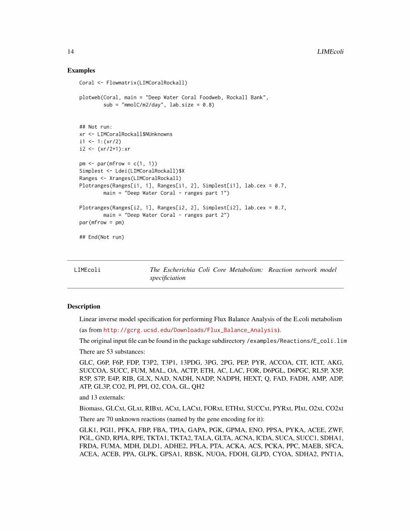
LIMEcoli The Escherichia Coli Core Metabolism: Reaction network modelspecificiation

Description

Linear inverse model specification for performing Flux Balance Analysis of the E.coli metabolism

(as from http://gcrg.ucsd.edu/Downloads/Flux_Balance_Analysis).

The original input file can be found in the package subdirectory /examples/Reactions/E_coli.lim

There are 53 substances:

GLC, G6P, F6P, FDP, T3P2, T3P1, 13PDG, 3PG, 2PG, PEP, PYR, ACCOA, CIT, ICIT, AKG,SUCCOA, SUCC, FUM, MAL, OA, ACTP, ETH, AC, LAC, FOR, D6PGL, D6PGC, RL5P, X5P,R5P, S7P, E4P, RIB, GLX, NAD, NADH, NADP, NADPH, HEXT, Q, FAD, FADH, AMP, ADP,ATP, GL3P, CO2, PI, PPI, O2, COA, GL, QH2

and 13 externals:

Biomass, GLCxt, GLxt, RIBxt, ACxt, LACxt, FORxt, ETHxt, SUCCxt, PYRxt, PIxt, O2xt, CO2xt

There are 70 unknown reactions (named by the gene encoding for it):

GLK1, PGI1, PFKA, FBP, FBA, TPIA, GAPA, PGK, GPMA, ENO, PPSA, PYKA, ACEE, ZWF,PGL, GND, RPIA, RPE, TKTA1, TKTA2, TALA, GLTA, ACNA, ICDA, SUCA, SUCC1, SDHA1,FRDA, FUMA, MDH, DLD1, ADHE2, PFLA, PTA, ACKA, ACS, PCKA, PPC, MAEB, SFCA,ACEA, ACEB, PPA, GLPK, GPSA1, RBSK, NUOA, FDOH, GLPD, CYOA, SDHA2, PNT1A,

http://gcrg.ucsd.edu/Downloads/Flux_Balance_Analysis

LIMEcoli 15

PNT2A, ATPA, GLCUP, GLCPTS, GLUP, RIBUP, ACUP, LACUP, FORUP, ETHUP, SUCCUP,PYRUP, PIUP, O2TX, CO2TX, ATPM, ADK, Growth

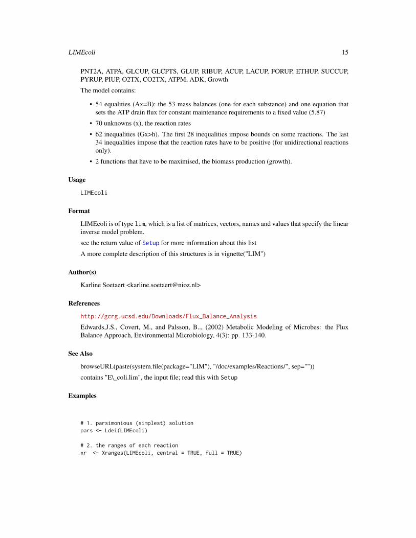
The model contains:

• 54 equalities (Ax=B): the 53 mass balances (one for each substance) and one equation thatsets the ATP drain flux for constant maintenance requirements to a fixed value (5.87)

• 70 unknowns (x), the reaction rates

• 62 inequalities (Gx>h). The first 28 inequalities impose bounds on some reactions. The last34 inequalities impose that the reaction rates have to be positive (for unidirectional reactionsonly).

• 2 functions that have to be maximised, the biomass production (growth).

Usage

LIMEcoli

Format

LIMEcoli is of type lim, which is a list of matrices, vectors, names and values that specify the linearinverse model problem.



Author(s)


References


Edwards,J.S., Covert, M., and Palsson, B.., (2002) Metabolic Modeling of Microbes: the FluxBalance Approach, Environmental Microbiology, 4(3): pp. 133-140.

See Also

browseURL(paste(system.file(package="LIM"), "/doc/examples/Reactions/", sep=""))

contains "E\_coli.lim", the input file; read this with Setup

Examples

# 1. parsimonious (simplest) solutionpars <- Ldei(LIMEcoli)

# 2. the ranges of each reactionxr <- Xranges(LIMEcoli, central = TRUE, full = TRUE)


16 LIMEverglades

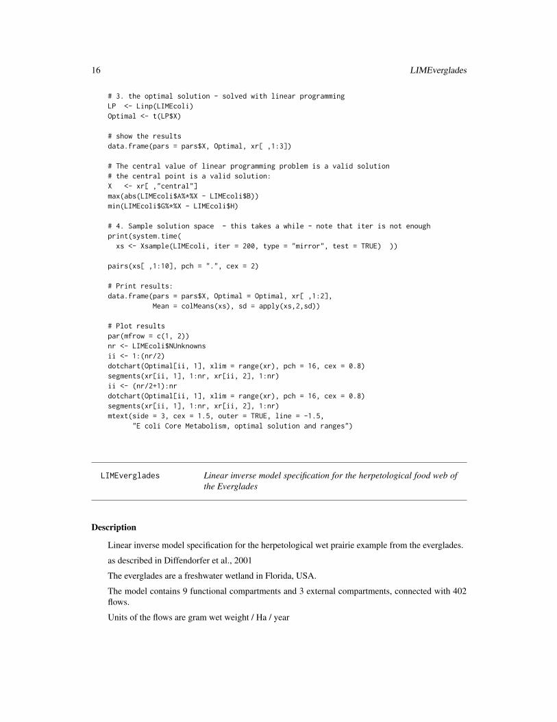
# 3. the optimal solution - solved with linear programmingLP <- Linp(LIMEcoli)Optimal <- t(LP$X)

# show the resultsdata.frame(pars = pars$X, Optimal, xr[ ,1:3])

# The central value of linear programming problem is a valid solution# the central point is a valid solution:X <- xr[ ,"central"]max(abs(LIMEcoli$A%*%X - LIMEcoli$B))min(LIMEcoli$G%*%X - LIMEcoli$H)

# 4. Sample solution space - this takes a while - note that iter is not enoughprint(system.time(

xs <- Xsample(LIMEcoli, iter = 200, type = "mirror", test = TRUE) ))

pairs(xs[ ,1:10], pch = ".", cex = 2)

# Print results:data.frame(pars = pars$X, Optimal = Optimal, xr[ ,1:2],

Mean = colMeans(xs), sd = apply(xs,2,sd))

# Plot resultspar(mfrow = c(1, 2))nr <- LIMEcoli$NUnknownsii <- 1:(nr/2)dotchart(Optimal[ii, 1], xlim = range(xr), pch = 16, cex = 0.8)segments(xr[ii, 1], 1:nr, xr[ii, 2], 1:nr)ii <- (nr/2+1):nrdotchart(Optimal[ii, 1], xlim = range(xr), pch = 16, cex = 0.8)segments(xr[ii, 1], 1:nr, xr[ii, 2], 1:nr)mtext(side = 3, cex = 1.5, outer = TRUE, line = -1.5,

"E coli Core Metabolism, optimal solution and ranges")

LIMEverglades Linear inverse model specification for the herpetological food web ofthe Everglades

Description

Linear inverse model specification for the herpetological wet prairie example from the everglades.

as described in Diffendorfer et al., 2001

The everglades are a freshwater wetland in Florida, USA.

The model contains 9 functional compartments and 3 external compartments, connected with 402flows.

Units of the flows are gram wet weight / Ha / year

LIMEverglades 17

The linear inverse model LIMEverglades is generated from the file Everglades.input which can befound in subdirectory /examples/FoodWeb of the package directory


These files can be read using Read and their output processed by Setup which will produce a linearinverse problem specification similar to LIMEverglades

Usage

data(LIMEverglades)

Format




Author(s)


References

Diffendorfer, J.E., Richards, P.M., Dalrymple, G.H., DeAngelis, D.L., 2001. Applying Linear Pro-gramming to estimate fluxes in ecosystems or food webs: an example from the herpetologicalassemblage of the freshwater Everglades. Ecol. Model. 144, 99-120.

See Also


contains "Everglades.input", the input file; read this with Setup


Examples

# Cannot be solved, but the least squares solution is foundFlows <- Lsei(LIMEverglades, parsimonious = TRUE)Everglades <- Flowmatrix(LIMEverglades)plotweb(Everglades, main = "Everglades Herpetological Wet Prairie model",

sub = "g WW/Ha/Yr", lab.size = 0.8)

18 LIMRigaAutumn

LIMRigaAutumn Linear inverse model specification for the Gulf of Riga *autumn*planktonic food web

Description

Linear inverse model specification for the Gulf of Riga planktonic food web in *autumn* as inDonali et al. (1999).

The Gulf of Riga is a highly eutrophic system in the Baltic Sea.

The foodweb comprises 7 functional compartments and two external compartments, connected with26 flows. Units of the flows are mg C/m3/day

The linear inverse model LIMRigaAutumn is generated from the file RigaAutumn.input which canbe found in subdirectory /examples/FoodWeb of the package directory


These files can be read using Read and their output processed by Setup which will produce a linearinverse problem specification similar to LIMRigaAutumn

Usage

data(LIMRigaAutumn)

Format




Author(s)


Dick van Oevelen<[email protected]>

References


See Also


contains "RigaAutumn.input", the input file; read this with Setup

LIMTakapoto, LIMRigaSummer, LIMRigaSpring and many others

LIMRigaSpring 19

Examples

rigaAutumn <- Flowmatrix(LIMRigaAutumn)plotweb(rigaAutumn, main = "Gulf of Riga planktonic food web, autumn",

sub = "mgC/m3/day")# ranges of flowsPlotranges(LIMRigaAutumn, lab.cex = 0.7, xlab = "mgC/m3/d",

main = "Gulf of Riga planktonic food web, autumn, Flowranges")# ranges of variablesPlotranges(LIMRigaAutumn, type="V", lab.cex = 0.7, xlab = "mgC/m3/d",

main = "Gulf of Riga planktonic food web, autumn, variables")

LIMRigaSpring Linear inverse model specification for the Gulf of Riga *spring* plank-tonic food web.

Description

Linear inverse model specification for the Gulf of Riga planktonic food web in *spring* as in Donaliet al. (1999).




The linear inverse model LIMRigaSpring is generated from the file RigaSpring.input which can befound in subdirectory /examples/FoodWeb of the package directory


These files can be read using Read and their output processed by Setup which will produce a linearinverse problem specification similar to LIMRigaSpring.

Usage

data(LIMRigaSpring)

Format




Author(s)


Dick van Oevelen<[email protected]>

20 LIMRigaSummer

References


See Also


contains "RigaSpring.input", the input file; read this with Setup

LIMTakapoto,LIMRigaAutumn, LIMRigaAutumn and many others

Examples

rigaSpring <- Flowmatrix(LIMRigaSpring)plotweb(rigaSpring, main = "Gulf of Riga planktonic food web, spring",

sub = "mgC/m3/day")Plotranges(LIMRigaSpring, lab.cex = 0.7,

main = "Gulf of Riga planktonic food web, spring, Flowranges")Plotranges(LIMRigaSpring, type = "V", lab.cex = 0.7,

main = "Gulf of Riga planktonic food web, spring, Variable ranges")

LIMRigaSummer Linear inverse model specification for the Gulf of Riga *summer*planktonic food web.

Description

Linear inverse model specification for the Gulf of Riga planktonic food web in *summer* as inDonali et al. (1999).




The linear inverse model LIMRigaSummer is generated from the file RigaSummer.input which canbe found in subdirectory /examples/FoodWeb of the package directory


These files can be read using Read and their output processed by Setup which will produce a linearinverse problem specification similar to LIMRigaSummer

Usage

data(LIMRigaSummer)

LIMScheldtIntertidal 21

Format


see the return value of Setup for more information about this list.


Author(s)


Dick van Oevelen <[email protected]>

References


See Also


contains "RigaSummer.input", the input file; read this with Setup

LIMTakapoto,LIMRigaAutumn, LIMRigaSpring and many others

Examples

rigaSummer <- Flowmatrix(LIMRigaSummer)plotweb(rigaSummer, sub = "mgC/m3/day",

main = "Gulf of Riga planktonic food web, summer")Plotranges(LIMRigaSummer, type = "V", lab.cex = 0.7,

main = "Gulf of Riga planktonic food web, summer, Variable ranges")

LIMScheldtIntertidal Linear inverse model specification for the Schelde Intertidal flat foodweb

Description

Linear inverse model specification for the Westerschelde Intertidal flat food web in June

as in Van Oevelen et al. (2006).

The Westerschelde is a highly eutrophic estuary in the Netherlands.

The food web model was created for the intertidal flat called the "Molenplaat", site 2.

It is the basic input model.

The foodweb comprises 7 functional compartments and five external compartments, connected with32 flows.


22 LIMScheldtIntertidal

The linear inverse model LIMScheldtIntertidal is generated from the file ScheldtIntertidal.input whichcan be found in subdirectory /examples/FoodWeb of the package directory


These files can be read using Read and their output processed by Setup which will produce a linearinverse problem specification similar to LIMScheldtIntertidal

Usage

data(LIMScheldtIntertidal)

Format




Author(s)

Karline Soetaert <[email protected]> Dick van Oevelen<[email protected]>

References

Van Oevelen, D., Soetaert, K., Middelburg, J.J., Herman, P.M.J., Moodley, L., Hamels, I., Moens,T., Heip, C.H.R., 2006b. Carbon flows through a benthic food web: Integrating biomass, isotopeand tracer data. J. Mar. Res. 64, 1-30.

See Also


contains "ScheldtIntertidal.input", the input file; read this with Setup


Examples

ScheldtIntertidal <- Flowmatrix(LIMScheldtIntertidal)plotweb(ScheldtIntertidal, main = "Scheldt intertidal flat food web",

sub = "mgC/m2/day")Plotranges(LIMScheldtIntertidal, lab.cex = 0.7,

main = "Scheldt intertidal flat food web, Flowranges")Plotranges(LIMScheldtIntertidal, type = "V", lab.cex = 0.7,

main = "Scheldt intertidal flat food web, Variable ranges")

LIMTakapoto 23

LIMTakapoto Linear inverse model specification for the Takapoto atoll planktonicfood web.

Description

Linear inverse model specification for the Carbon flux model of the Takapoto atoll planktonic foodweb

as reconstructed by inverse modelling by Niquil et al. (1998).

The Takapoto Atoll lagoon is located in the French Polynesia of the South Pacific

The food web comprises 7 functional compartments and three external compartments/sinks con-nected with 32 flows.


The linear inverse model LIMTakapoto is generated from the file Takapoto.input which can befound in subdirectory /examples/FoodWeb of the package directory


These files can be read using Read and their output processed by Setup which will produce a linearinverse problem specification similar to LIMTakapoto

Usage

data(LIMTakapoto)

Format




Author(s)

Karline Soetaert <[email protected]> Dick van Oevelen<[email protected]>

References

Niquil, N., Jackson, G.A., Legendre, L., Delesalle, B., 1998. Inverse model analysis of the plank-tonic food web of Takapoto Atoll (French Polynesia). Marine Ecology Progress Series 165, 17..29.

See Also


contains "Takapoto.input", the input file; read this with Setup

LIMRigaAutumn and many others

24 Linp

Examples

Takapoto <- Flowmatrix(LIMTakapoto)plotweb(Takapoto, main="Takapoto atoll planktonic food web",

sub = "mgC/m2/day", lab.size = 1)# some ranges extend to infinity - they are marked with "*"Plotranges(LIMTakapoto, lab.cex = 0.7,

sub = "*=unbounded", xlab = "mgC/m2/d",main = "Takapoto atoll planktonic food web, Flowranges")

# ranges of variables, exclude firstPlotranges(LIMTakapoto, type = "V", lab.cex = 0.7,

index = 2:23, xlab = "mgC/m2/d",main = "Takapoto atoll planktonic food web, Variable ranges")

Linp Solves a linear inverse model using linear programming.

Description

Solves a linear inverse model using linear programming

Input presented either as:

• matrices E, F, A, B, G, H (Linp.double) or

• as a list (Linp.lim) or

• as a lim input file (Linp.limfile)

Usage

Linp(...)## S3 method for class 'lim'Linp(lim, cost = NULL, ispos = lim$ispos, ...)## S3 method for class 'limfile'Linp(file, verbose = TRUE,...)## S3 method for class 'character'Linp(...)## S3 method for class 'double'Linp(...)

Arguments


file name of the inverse input file.

verbose if TRUE: when reading the file, prints warnings and messages to the screen.

cost if not NULL, a vector with the coefficients of the cost function (to be minimised).

ispos if TRUE: all x-values have to be positive.

... other arguments passed to function linp from packagelimSolve.

Linp 25

Details


min(∑

Costi ∗ xi)

ormax(

∑Profiti ∗ xi)

subject toxi >= 0

Ax = B

Gx >= H

and where Costi or Profiti are weighting coefficients

Value

a list containing:

X vector containing the solution of the linear programming problem.unconstrained.solution

vector containing the unconstrained solution of the linear programming prob-lem.

residualNorm scalar, the sum of residuals of equalities and violated inequalities.

solutionNorm scalar, the value of the quadratic function at the solution.

IsError logical, TRUE if an error occurred.

Error linp error text.

type linp.

Author(s)


References

Michel Berkelaar and others (2005). lpSolve: Interface to Lpsolve v. 5 to solve linear/integerprograms. R package version 1.1.9.

See Also

linp, the more general function from package lpSolve

Ldei, to solve the linear inverse problem by least distance programming

Lsei, to solve the linear inverse problem by lsei (least squares with equality and inequality con-straints)

function linp from packagelimSolve

26 Lsei

Examples

# the Blending exampleLinp(LIMBlending)

# the E coli example: two functions to maximimiseLinp(LIMEcoli)

# E coli example, but only first function optimised..Linp(LIMEcoli, cost = -LIMEcoli$Profit[1,])

# a foodweb example: need to specify the cost function# here just sum of absolute values of flows...Linp(LIMRigaAutumn, cost = (rep(1, LIMRigaAutumn$NUnknowns)))

Lsei Solves a linear inverse model using the least squares method.

Description

Solves a linear inverse model using the least squares method

Input presented as:

• matrices E, F, A, B, G, H (Lsei.double) or

• a list (Lsei.lim) or

• as a lim input file (Lsei.limfile)

Useful for solving overdetermined lims.

Usage

Lsei(...)## S3 method for class 'double'Lsei(...)## S3 method for class 'lim'Lsei(lim, exact = NULL, parsimonious = FALSE, ...)## S3 method for class 'limfile'Lsei(file, exact = NULL, parsimonious = FALSE,

verbose = TRUE, ...)## S3 method for class 'character'Lsei(...)

Arguments


exact if not NULL, a vector containing the numbers of the equations to be solved ex-actly; if NULL, all equations are considered exact.

Lsei 27

parsimonious if TRUE, also minimises the sum of squared unknowns.


verbose if TRUE: when reading the file, prints warnings and messages to the screen.

... other arguments passed to function lsei from packagelimSolve.

Details


min(||AAx−BB||2)

, the approximate equations subject toEx = F

, the mass balancesGx >= H

, the constraints.

and where E and F make up the equations from A and B, as specified by vector exact.

AA and BB are the equations from A and B, NOT in vector exact.

in case exact = NULL, there are no approximate equations.

in case parsimonious = TRUE, then the sum of squared unknowns is also minimised. This meansthat AA is augmented with the unity matrix (of size Nunknowns) and BB contains Nunknowns addi-tional zeros.

For overdetermined lim problems, for instance, the inverse equations may be split up in the massbalance equations which have to be exactly met and the other equations which have to be approxi-mated.

This is, it is assumed that the first *NComponents* equations, the mass balances, should be metexactly and the call to the function is: Lsei(lim,exact = 1:lim$NComponents,...)

If the lim is underdetermined, an alternative is to use Ldei instead.

This will return the parsimonious solution.

The results should be similar with Lsei(...,parsimonious=TRUE).

In theory both Lsei.lim and Ldei should return the same value for underdetermined systems.

Value

a list containing:

X vector containing the solution of the least squares problem.

residualNorm scalar, the sum of residuals of equalities and violated inequalities.

solutionNorm scalar, the value of the minimised quadratic function at the solution.

IsError TRUE if an error occurred.

Error error text.

type lsei.

28 Plotranges

Author(s)


References

K. H. Haskell and R. J. Hanson, An algorithm for linear least squares problems with equality andnonnegativity constraints, Report SAND77-0552, Sandia Laboratories, June 1978.

K. H. Haskell and R. J. Hanson, Selected algorithms for the linearly constrained least squares prob-lem - a users guide, Report SAND78-1290, Sandia Laboratories,August 1979.

K. H. Haskell and R. J. Hanson, An algorithm for linear least squares problems with equality andnonnegativity constraints, Mathematical Programming 21 (1981), pp. 98-118.

R. J. Hanson and K. H. Haskell, Two algorithms for the linearly constrained least squares problem,ACM Transactions on Mathematical Software, September 1982.

See Also

lsei, the more general function from package limSolve

Linp, to solve the linear inverse problem by linear programming

Ldei, to solve the linear inverse problem by least distance programming

function lsei from packagelimSolve

Examples

Lsei(LIMRigaAutumn, parsimonious = TRUE)

Plotranges Plots the minimum and maximum and central values

Description

Plots minimum and maximum ranges.

Takes as input either a lim list, as generated by Setup or a set of vectors specifying the minimum,maximum and the central value, or a data.frame that contains min, max and central values.

Usage

Plotranges(...)## S3 method for class 'double'Plotranges(min, max, value = NULL, labels = NULL, log = "",pch = 16, pch.col = "black", line.col = "gray",seg.col = "black", xlim = NULL, main = NULL,xlab = NULL, ylab = NULL, lab.cex = 1.0, mark = NULL,...)

## S3 method for class 'lim'Plotranges(lim = NULL, labels = NULL, type = "X", log = "",

Plotranges 29

pch = 16, pch.col = "black", line.col = "gray",seg.col = "black", xlim = NULL, main = NULL,xlab = NULL, ylab = NULL, lab.cex = 1.0, index = NULL, ...)

## S3 method for class 'character'Plotranges(file, ...)

Arguments

min minimum value.

max maximum value.

value median or mean value.



labels names of each value.

type one of "X" or "V" for plotting of unknowns (X) or variables.

log if = x: logarithmic scale for x-axis.

pch pch symbol used for mean value.

pch.col pch color for mean value.

line.col color for each variable, spanning x-axis.

seg.col color for variable range.

xlim limits on x-axis.

main main title.

xlab x-axis label.

ylab y-axis label.

lab.cex label expansion value.

index list of elements to be plotted, a vector of integers; default = all elements.

mark list of elements to be marked with a "*", i.e. when range is unbounded.

... arguments passed to R-function "text" when writing labels.

Value

Only when a lim list was inputted. A data frame with

min the minimum.

max the maximum.

values the central value.

Author(s)


30 PrintMat

Examples

# The Takapoto food web.# some ranges extend to infinity - they are marked with "*"Plotranges(LIMTakapoto, lab.cex = 0.7, sub = "*=unbounded",

xlab = "mgC/m2/d",main = "Takapoto atoll planktonic food web, Flowranges")

# ranges of variables, exclude first variablePlotranges(LIMTakapoto, type = "V", lab.cex = 0.7,

index = 2:23, xlab = "mgC/m2/d",main = "Takapoto atoll planktonic food web, Variable ranges")

PrintMat Writes linear inverse matrices to the screen

Description

Prints the linear inverse problem:

• inverse matrices and vectors A, b of the equalities

Ax = b

• inverse matrices and vectors G, h of the inequalities

Gx >= h

• if present, also writes the cost/profit function

Usage

PrintMat(lim)

Arguments


Value

returns nothing.

Author(s)


Examples

PrintMat(LIMBlending)

Read 31

Read Reads an inverse input file

Description

Reads an inverse input file and creates the inverse problem as a list, of type "liminput"

Usage

Read(file, verbose = FALSE, checkLinear = TRUE, remtabs = TRUE)

Arguments

file name of inverse input file.

verbose if TRUE: prints warnings and messages to the screen.

checkLinear if FALSE: does not check for linearity

remtabs remove tabs.

Details

The structure of an inverse input file is explained in vignette("LIM") which should be consulted.

In short the inverse input file contains the declaration sections enclosed inbetween two lines startingwith a \#\#.

For instance, the following section declares two components

\# COMP

State1

State2

\# END COMP

Only the first 4 characters of the section names are read

The following sections are allowed:

• Parameters - \#\# PARAMETERS

• Components - \#\# STOCKS or \#\# DECISION VARIABLES or \#\# STATES or \#\# UN-KNOWNS

• Externals - \#\# EXTERNALS

• Rates - \#\# RATES

• Flows - \#\# FLOWS

• Variables - \#\# VARIABLES

• Cost - \#\# COST or \#\# MINIMISE

• Profit - \#\# PROFIT or \#\# MAXIMISE

• Equalities - \#\# EQUALITIES

32 Read

• InEqualities - \#\# INEQUALITIES or \#\# CONSTRAINTS

Any (part of a) line starting with a "!" is considered a comment.

Input is NOT case sensitive

The output of this function is used as input in function Setup which creates the inverse matrices

By default, only linear problems can be solved, and the function checks whether the input is linear.To toggle off this check, set checkLinear to FALSE.

Some input files contain tabs, which are converted to spaces, unless this logical is set to FALSE.

Value

a list containing :


pars a data.frame with parameter declarations.

comp a data.frame with compartments (or states, stocks).

rate a data.frame with rate declarations.

extern a data.frame with external declarations.

flows a data.frame with flow declarations.

vars a data.frame with variable declarations.

cost a data.frame with cost declarations.

profit a data.frame with profit declarations.

equations a data.frame with equality declarations.

constraints a data.frame with constraint declarations.

reactions a data.frame with reaction declarations.

posreac a vector with TRUE values if reaction or flow is unidirectional (and the unknownx is thus positive), FALSE if it is two-way reaction or flow, and x can be positiveor negative.

marker a data.frame with marker declarations - see vignette("LIM").

parnames a vector with parameter names.

varnames a vector with variable names.

compnames a vector with compartment names.

externnames a vector with names of externals.

Type a string; one of "web" (flows are unknowns), "reaction" (reaction rates unknown)and "simple" (compartments are unknowns).

Author(s)


See Also

Setup the function to create inverse matrices, based on output of Read.

Setup 33

Examples

# this input has been created with function Read:LIMinputBlending

## Not run:wd <- getwd()setwd(paste(system.file(package = "LIM"), "/doc/examples/Foodweb", sep = ""))Read("RigaAutumn.input")setwd(wd)

## End(Not run)

Setup Creates linear inverse matrices

Description

Creates the linear problem with equality and inequality equations.

Takes as input either a liminput list, as generated by Read or a filename with the linear inversemodel specifications. Creates:

• inverse matrices and vectors A, b, G, h of the equalities/inequalities:

Ax = b

Gx >= h

• if present, also generates the cost/profit function which is used as:

min(cost)

ormax(profit)

• if the input was a flow network, Setup will also create the flow matrix (see details).

Usage

Setup(...)## S3 method for class 'limfile'Setup(file, verbose = TRUE, ...)## S3 method for class 'character'Setup(...)## S3 method for class 'liminput'Setup(liminput,...)

34 Setup

Arguments


verbose if TRUE: prints warnings and messages to the screen.

liminput list of elements, as returned by Read.

... extra parameters allowing this to be a generic function.

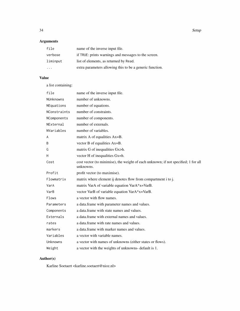
Value

a list containing:


NUnknowns number of unknowns.

NEquations number of equations.

NConstraints number of constraints.

NComponents number of components.

NExternal number of externals.

NVariables number of variables.

A matrix A of equalities Ax=B.

B vector B of equalities Ax=B.

G matrix G of inequalities Gx>h.

H vector H of inequalities Gx=h.

Cost cost vector (to minimise), the weight of each unknown; if not specified; 1 for allunknowns.

Profit profit vector (to maximise).

Flowmatrix matrix where element ij denotes flow from compartment i to j.

VarA matrix VarA of variable equation VarA*x=VarB.

VarB vector VarB of variable equation VarA*x=VarB.

Flows a vector with flow names.

Parameters a data.frame with parameter names and values.

Components a data.frame with state names and values.

Externals a data.frame with external names and values.

rates a data.frame with rate names and values.

markers a data.frame with marker names and values.

Variables a vector with variable names.

Unknowns a vector with names of unknowns (either states or flows).

Weight a vector with the weights of unknowns- default is 1.

Author(s)


Variables 35

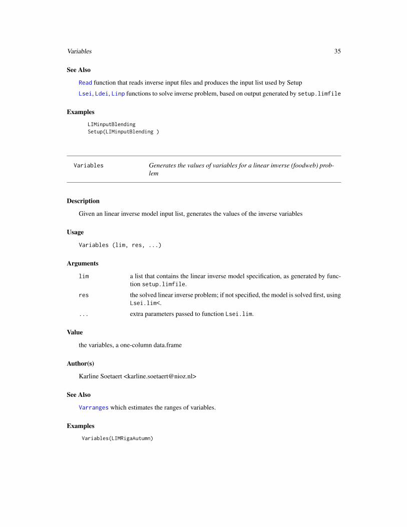
See Also

Read function that reads inverse input files and produces the input list used by Setup

Lsei, Ldei, Linp functions to solve inverse problem, based on output generated by setup.limfile

Examples

LIMinputBlendingSetup(LIMinputBlending )

Variables Generates the values of variables for a linear inverse (foodweb) prob-lem

Description

Given an linear inverse model input list, generates the values of the inverse variables

Usage

Variables (lim, res, ...)

Arguments


res the solved linear inverse problem; if not specified, the model is solved first, usingLsei.lim<.

... extra parameters passed to function Lsei.lim.

Value

the variables, a one-column data.frame

Author(s)


See Also

Varranges which estimates the ranges of variables.

Examples

Variables(LIMRigaAutumn)

36 Varranges

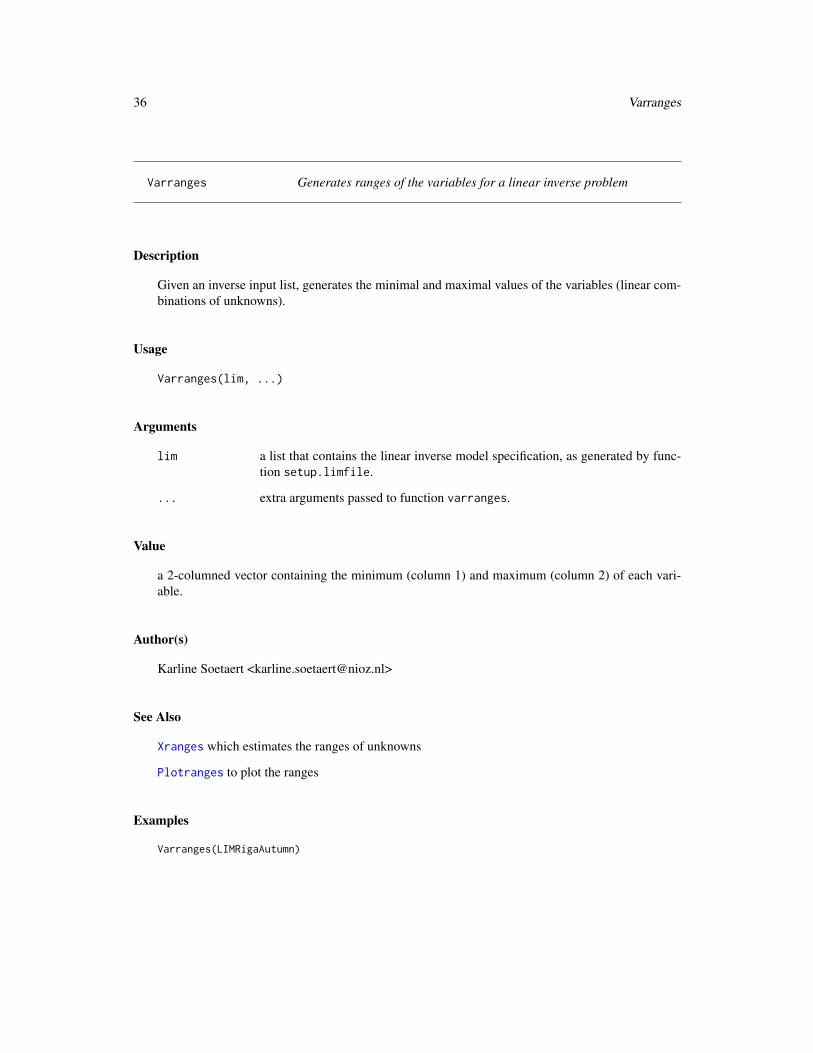
Varranges Generates ranges of the variables for a linear inverse problem

Description

Given an inverse input list, generates the minimal and maximal values of the variables (linear com-binations of unknowns).

Usage

Varranges(lim, ...)

Arguments


... extra arguments passed to function varranges.

Value

a 2-columned vector containing the minimum (column 1) and maximum (column 2) of each vari-able.

Author(s)


See Also

Xranges which estimates the ranges of unknowns

Plotranges to plot the ranges

Examples

Varranges(LIMRigaAutumn)

Xranges 37

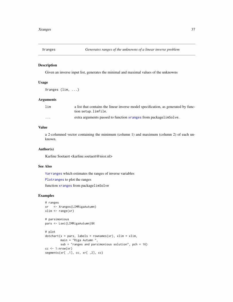
Xranges Generates ranges of the unknowns of a linear inverse problem

Description

Given an inverse input list, generates the minimal and maximal values of the unknowns

Usage

Xranges (lim, ...)

Arguments


... extra arguments passed to function xranges from packagelimSolve.

Value

a 2-columned vector containing the minimum (column 1) and maximum (column 2) of each un-known.

Author(s)


See Also

Varranges which estimates the ranges of inverse variables


function xranges from packagelimSolve

Examples

# rangesxr <- Xranges(LIMRigaAutumn)xlim <- range(xr)

# parsimoniouspars <- Lsei(LIMRigaAutumn)$X

# plotdotchart(x = pars, labels = rownames(xr), xlim = xlim,

main = "Riga Autumn ",sub = "ranges and parsimonious solution", pch = 16)

cc <- 1:nrow(xr)segments(xr[ ,1], cc, xr[ ,2], cc)

38 Xsample

Xsample Generates a random sample of the unknowns for a linear inverse prob-lem

Description

Given an inverse input list, randomly samples the unknowns, using an MCMC method

Usage

Xsample(lim, exact = NULL, ...)

Arguments


exact if not NULL, a vector containing the numbers of the equations to be solved ex-actly; if NULL, all equations are considered exact.

... extra parameters passed to function xsample from packagelimSolve.

Details

For overdetermined LIM problems, the inverse equations may be split up in equations which haveto be exactly met and other equations which have to be approximated.

exact is a vector with the exact equations

The default settings of xsample will often not do. For instance, the default consists of 3000 itera-tions (iter) and a jump length of jmp of 0.1. You may need to increase one of those to ensure thatthe entire solution space has been adequately sampled.

Value

a 2-columned vector containing the minimum (column 1) and maximum (column 2) of each un-known.

Author(s)


References

Van den Meersche K, Soetaert K, Van Oevelen D (2009). xsample(): An R Function for SamplingLinear Inverse Problems. Journal of Statistical Software, Code Snippets, 30(1), 1-15.

http://www.jstatsoft.org/v30/c01/

http://www.jstatsoft.org/v30/c01/

Xsample 39

See Also

Varranges which estimates the ranges of inverse variables


function xsample from packagelimSolve

Examples

# sample solution spacexs <- Xsample(LIMRigaAutumn, iter = 500, jmp = 5)# remove flows that are invariable (sd=0)xs <- xs[ ,-which(apply(xs, 2, sd) == 0 )]#pairs plotpairs(xs, gap = 0, pch = ".", upper.panel = NULL)

Index

∗Topic IOPrintMat, 30Read, 31Setup, 33

∗Topic algebraLdei, 6Linp, 24Lsei, 26

∗Topic arrayLdei, 6Linp, 24Lsei, 26

∗Topic datasetsFILERigaAutumn, 4LIMBlending, 8LIMBrouageMudflat, 10LIMCaliforniaSediment, 11LIMCoralRockall, 13LIMEcoli, 14LIMEverglades, 16LIMRigaAutumn, 18LIMRigaSpring, 19LIMRigaSummer, 20LIMScheldtIntertidal, 21LIMTakapoto, 23

∗Topic hplotPlotranges, 28

∗Topic optimizeLdei, 6Linp, 24Lsei, 26Varranges, 36Xranges, 37Xsample, 38

∗Topic packageLIM-package, 2

∗Topic utilitiesFlowmatrix, 5PrintMat, 30

Setup, 33Variables, 35Varranges, 36Xranges, 37Xsample, 38

FILERigaAutumn, 4Flowmatrix, 3, 5

Ldei, 3, 6, 25, 27, 28, 35ldei, 7LIM (LIM-package), 2LIM-package, 2LIMBlending, 8LIMBrouageMudflat, 10LIMCaliforniaSediment, 11LIMCoralRockall, 13LIMEcoli, 9, 14LIMEverglades, 16LIMinputBlending (LIMBlending), 8LIMRigaAutumn, 5, 18, 20, 21, 23LIMRigaSpring, 18, 19, 21LIMRigaSummer, 11–13, 17, 18, 20, 22LIMScheldtIntertidal, 21LIMTakapoto, 9, 11–13, 17, 18, 20–22, 23Linp, 3, 7, 24, 28, 35linp, 24, 25Lsei, 3, 7, 25, 26, 35lsei, 27, 28

Plotranges, 3, 28, 36, 37, 39plotweb, 6PrintMat, 30

Read, 3, 4, 9–11, 17–20, 22, 23, 31, 35

Setup, 3, 4, 9–13, 15, 17–23, 32, 33

Variables, 3, 35Varranges, 3, 35, 36, 37, 39

40

INDEX 41

Xranges, 3, 36, 37xranges, 37Xsample, 3, 38xsample, 38, 39

Documents

Package ‘LIM’ - The Comprehensive R Archive Network lim ... (package="LIM"), "/doc/examples/Foodweb ... Mathematically this can be estimated by solving a linear programming problem: