Embed Size (px)
Citation preview

PACKAGE NP FAQ
JEFFREY S. RACINE
Contents
1. Overview and Current Version 42. Frequently Asked Questions 52.1. How do I cite the np package? 52.2. I have never used R before. Can you direct me to some introductory material
that will guide me through the basics? 62.3. How do I keep all R packages on my system current? 62.4. It seems that there are a lot of packages that must be installed in order to
conduct econometric analysis (tseries, lmtest, np, etc.). Is there a way toavoid having to individually install each package individually? 6
2.5. Is there a ‘gentle guide’ to the np package that contains some easy to followexamples? 7
2.6. I noticed you have placed a new version of the np package on CRAN. How canI determine what has been changed, modified, fixed etc? 7
2.7. What is the difference between the np package and the previous stand-aloneprograms you wrote, namely, N ©, NPREG ©, and NPDEN ©? 7
2.8. How can I read data stored in various formats such as Stata, SAS, Minitab,SPSS etc. into the R program? 8
2.9. I want to use so-and-so’s semiparametric/nonparametric method, however, thenp package does not include this particular method. . . 8
2.10. Cross-validation takes forever, and I can’t wait that long. . . 82.11. Is there a way to figure out roughly how long cross-validation will take on a
large sample? 132.12. Where can I get some examples of R code for the np package in addition to
the examples in the help files? 142.13. I need to apply a boundary correction for a univariate density estimate - how
can I do this? 152.14. I notice your density estimator supports manual bandwidths, the normal-
reference rule-of-thumb, likelihood cross-validation and least squarescross-validation, but not plug-in rules. How can I use various plug-in rulesfor estimating a univariate density? 15
2.15. I wrote a program using np and it does not work as I expected. . . 152.16. Under Mac OS X, when I run a command no progress is displayed. . . 16
Date: June 4, 2018.
1
2 JEFFREY S. RACINE
2.17. When some routines are running under MS Windows, R appears to be ‘notresponding.’ It appears that the program is not ‘hung’, rather is simplycomputing. The previous stand-alone program (N ©) always displayeduseful information. . . 16
2.18. Some results take a while, and my MS Windows computer is sluggish while R
is running. . . 162.19. A variable must be cast as, say, a factor in order for np to recognize this as an
unordered factor. How can I determine whether my data is already castas a factor? 17
2.20. When I use plot() (npplot()) existing graphics windows are overwritten.How can I display multiple graphics plots in separate graphics windowsso that I can see results from previous runs and compare that to my newrun? 17
2.21. Sometimes plot() fails to use my variable names. . . 172.22. Sometimes plot() appends my variable names with .ordered or .factor. . . 172.23. I specify a variable as factor() or ordered() in a data frame, then call this
when I conduct bandwidth selection. However, when I try to plot theresulting object, it complains with the following message: 17
2.24. My np code produces errors when I attempt to run it. . . 182.25. I have (numeric) 0/1 dummy variable regressors in my parametric model. Can
I just pass them to the np functions as I would in a parametric setting? 182.26. I have a categorical variable, ignored the advice in items 2.19 and 2.25, and R
terminates with the following error. 182.27. Rgui appears to crash. There must be a bug in the program. 182.28. Can I skip creating a bandwidth object and enter a bandwidth directly? 192.29. When I estimate my gradients and there are two or more covariates and then
extract them with the gradients() function, they are not ‘smooth’,though if I plot a model with the gradients=TRUE option, they are. Thegradients() function must be broken. . . 19
2.30. I use plot() (npplot()) to plot, say, a density and the resulting plot lookslike an inverted density rather than a density. . . 20
2.31. Can npksum() compute analytical derivatives with respect to a continuousvariable? 21
2.32. Can I use the npcmstest() function that implements the consistent testfor correct specification of parametric regression models as describedin Hsiao, Li, & Racine (2007) [6] to test for correct specification of thesemiparametric partially linear model? 22
2.33. I am using npcmstest() on a glm() object (the document says glm() objectsare supported and I am estimating a Logit model) but it returns an errorsaying 23
2.34. I want to plot the kernel function itself. How can I do this? 232.35. In version 0.20-0 and up I can ‘combine’ steps such as bandwidth selection and
estimation. But when I do summary(model) I don’t get the same summary

PACKAGE NP FAQ 3
that I would get from, say, summary(bw) and then summary(model). Howdo I get bandwidth object summaries when combining steps? 23
2.36. I estimated a semiparametric index model via model <- npindex(y~x1+x2)
but se(model) returns NULL 242.37. How do I interpret gradients from the conditional density estimator? 252.38. When I run R in batch mode via R CMD BATCH filename.R unwanted status
messages (e.g., “‘Multistart 1 of 10”’) crowd out desired output. How canI turn off these unwanted status messages? 25
2.39. I am getting an ‘unable to allocate...’ message after repeatedly interruptinglarge jobs. 25
2.40. I have a large number of variables, and when using the formula interface I getan error message stating ‘invoked with improper formula’. I have doublechecked and everything looks fine. Furthermore, it works fine with thedata frame interface. 25
2.41. How can I estimate additive semiparametric models? 262.42. I am using npRmpi and am getting an error message involving dlopen() 262.43. I am using the npRmpi package but when I launch one of the demo parallel jobs
I get the error Error: could not find function "mpi.bcast.cmd" 272.44. I have estimated a partially linear model and want to extract the gradient/fitted
values of the nonparametric component 272.45. The R function ‘lag()’ does not work as I expect it to. How can I create the lth
lag of a numeric variable in R to be fed to functions in the np package? 292.46. Can I provide sample weights to be used by functions in the np package? 302.47. Quantile regression is slow, particularly for very small/large values of tau. Can
this be sped up? 302.48. How can I generate resamples from the unknown distribution of a set of data
based on my smooth kernel density estimate? 322.49. Some of my variables are measured with an unusually large number of
digits. . . should I rescale? 322.50. The local linear gradient estimates appear to be somewhat ‘off’ in that they do
not correspond to the first derivative of the estimated regression function. 332.51. How can I turn off all console I/O? 332.52. Is there a way to exploit the sparse nature of the design matrix when all
predictors are categorical and reduce computation time, particularly forcross-validation? 34
2.53. I want to bootstrap the standard errors for the coefficients in a varyingcoefficient specification. Is there a simple way to accomplish this? 37
References 39Changes from Version 0.60-7 to 0.60-8 [04-Jun-2018] 40Changes from Version 0.60-6 to 0.60-7 [01-May-2018] 40Changes from Version 0.60-5 to 0.60-6 [12-Jan-2018] 40Changes from Version 0.60-4 to 0.60-5 [04-Jan-2018] 40Changes from Version 0.60-3 to 0.60-4 [03-Dec-2017] 40Changes from Version 0.60-2 to 0.60-3 [29-Apr-2017] 41

4 JEFFREY S. RACINE
Changes from Version 0.60-1 to 0.60-2 [27-Jun-2014] 41Changes from Version 0.60-0 to 0.60-1 [6-Jun-2014] 41Changes from Version 0.50-1 to 0.60-0 [1-Jun-2014] 42Changes from Version 0.40-13 to 0.50-1 [13-Mar-2013] 43Changes from Version 0.40-12 to 0.40-13 [05-Mar-2012] 44Changes from Version 0.40-11 to 0.40-12 [24-Nov-2011] 44Changes from Version 0.40-10 to 0.40-11 [24-Oct-2011] 44Changes from Version 0.40-9 to 0.40-10 [24-Oct-2011] 44Changes from Version 0.40-8 to 0.40-9 [30-July-2011] 45Changes from Version 0.40-7 to 0.40-8 [29-July-2011] 45Changes from Version 0.40-6 to 0.40-7 [8-Jun-2011] 45Changes from Version 0.40-5 to 0.40-6 [1-Jun-2011] 45Changes from Version 0.40-4 to 0.40-5 [26-Apr-2011] 45Changes from Version 0.40-3 to 0.40-4 [21-Jan-2011] 45Changes from Version 0.40-1 to 0.40-3 [23-Jul-2010] 46Changes from Version 0.40-0 to 0.40-1 [4-Jun-2010] 46Changes from Version 0.30-9 to 0.40-0 [25-May-2010] 46Changes from Version 0.30-8 to 0.30-9 [17-May-2010] 46Changes from Version 0.30-7 to 0.30-8 [20-Apr-2010] 47Changes from Version 0.30-6 to 0.30-7 [15-Feb-2010] 47Changes from Version 0.30-5 to 0.30-6 [3-Feb-2010] 47Changes from Version 0.30-4 to 0.30-5 [29-Jan-2010] 47Changes from Version 0.30-3 to 0.30-4 [27-Jan-2010] 47Changes from Version 0.30-2 to 0.30-3 [28-May-2009] 48Changes from Version 0.30-1 to 0.30-2 [19-Apr-2009] 48Changes from Version 0.30-0 to 0.30-1 [29-Jan-2009] 48Changes from Version 0.20-4 to 0.30-0 [15-Jan-2009] 48Changes from Version 0.20-3 to 0.20-4 [19-Nov-2008] 49Changes from Version 0.20-2 to 0.20-3[14-Nov-2008] 49Changes from Version 0.20-1 to 0.20-2 [02-Nov-2008] 49Changes from Version 0.20-0 to 0.20-1 [13-Aug-2008] 50Changes from Version 0.14-3 to 0.20-0 [28-Jul-2008] 50Changes from Version 0.14-2 to 0.14-3 [02-May-2008] 50Changes from Version 0.14-1 to 0.14-2 [11-Jan-2008] 50Changes from Version 0.13-1 to 0.14-1 [18-Dec-2007] 51Changes from Version 0.12-1 to 0.13-1 [03-May-2007] 51Version 0.12-1 [19-Nov-2006] 52
1. Overview and Current Version
This set of frequently asked questions is intended to help users who are encountering
unexpected or undesired behavior when trying to use the np package.

PACKAGE NP FAQ 5
Many of the underlying C routines have been extensively tested over the past two decades.
However, the R ‘hooks’ needed to call these routines along with processing of the data required
for a seamless user experience may produce unexpected or undesired results in some settings.
If you encounter any issues with the np package, kindly first ensure that you have the most
recent version of np, R, and RStudio (if appropriate) installed. Sometimes issues encountered
using outdated versions of software have been resolved in the current versions, so this is the
first thing one ought to investigate when the unexpected occurs.
Having ensured that the problem persists with the most recently available versions of all
software involved, kindly report any issues you encounter to me, and please include your
code, data, version of the np package, version of R, and operating system (with version
number) used so that I can help track down any such issues ([email protected]). And, of
course, if you encounter an issue that you think might be of interest to others, kindly email
me the relevant information and I will incorporate it into this FAQ.
This FAQ refers to the most recent version, which as of this writing is 0.60-8. Kindly
update your version should you not be using the most current (from within R, up-
date.packages() ought to do it, though also see 2.3 below.). See the appendix in this
file for cumulative changes between this and previous versions of the np package.
2. Frequently Asked Questions
2.1. How do I cite the np package? Once you have installed the np package
(install.packages("np")), if you load the np package (library("np")) and type ci-
tation("np") you will be presented with the following information.
> citation("np")
To cite np in publications use:
Tristen Hayfield and Jeffrey S. Racine (2008). Nonparametric
Econometrics: The np Package. Journal of Statistical Software
27(5). URL http://www.jstatsoft.org/v27/i05/.
A BibTeX entry for LaTeX users is
@Article{,
title = {Nonparametric Econometrics: The np Package},
author = {Tristen Hayfield and Jeffrey S. Racine},
journal = {Journal of Statistical Software},
year = {2008},
volume = {27},

6 JEFFREY S. RACINE
number = {5},
url = {http://www.jstatsoft.org/v27/i05/},
}
2.2. I have never used R before. Can you direct me to some introductory material
that will guide me through the basics? There are many excellent introductions to the R
environment with more on the way. First, I would recommend going directly to the R website
(http://www.r-project.org) and looking under Documentation/Manuals (http://cran.
r-project.org/manuals.html) where you will discover a wealth of documentation for R
users of all levels. See also the R task views summary page (http://cran.r-project.org/
web/views) for information grouped under field of interest. A few documents that I mention
to my students which are tailored to econometricians include http://cran.r-project.org/
doc/contrib/Verzani-SimpleR.pdf, Cribari-Neto & Zarkos (1999) [1], Racine & Hyndman
(2002) [11] and Farnsworth (2006) [3], to name but a few.
Those looking for exemplar data sets outside of those contained in the np package are
directed to the Ecdat [2] and AER [7] packages.
I maintain a ‘Gallery’ to provide a forum for users to share code and discover examples
and illustrations which can be found at http://socserv.mcmaster.ca/racinej/Gallery/
Home.html.
Often the best resource is right down the hall. Ask a colleague whether they use or know
anyone who uses R, then offer to buy that person a coffee and along the way drop something
like “I keep hearing about the R project. . . I feel like such a Luddite. . . ”
2.3. How do I keep all R packages on my system current? Run the command up-
date.packages(checkBuilt=TRUE,ask=FALSE), which will not only update all packages
that are no longer current, but will also update all packages built under outdated installed
versions of R, if appropriate.
2.4. It seems that there are a lot of packages that must be installed in order to
conduct econometric analysis (tseries, lmtest, np, etc.). Is there a way to avoid
having to individually install each package individually? Certainly. The Compre-
hensive R Archive Network (CRAN) is a network of ftp and web servers around the world
that store identical, up-to-date, versions of code and documentation for R. The CRAN ‘task
view’ for computational econometrics might be of particular interest to econometricians. The
econometric task view provides an excellent summary of both parametric and nonparametric
econometric packages that exist for the R environment and provides one-stop installation for
these packages.

PACKAGE NP FAQ 7
See cran.r-project.org/web/views/Econometrics.html for further information.
To automatically install a task view, the ctv package first needs to be installed and loaded,
i.e.,
install.packages("ctv")
library("ctv")
The econometric task view can then be installed via install.views() and updated via
update.views() (which first assesses which of the packages are already installed and up-to-
date), i.e.,
install.views("Econometrics")
or
update.views("Econometrics")
2.5. Is there a ‘gentle guide’ to the np package that contains some easy to
follow examples? Perhaps the most gentle introduction is contained in the np package
itself in the form of a ‘vignette’. To view the vignette run R, install the np package
(install.packages("np")), then type vignette("np",package="np") to view or print the
vignette (this vignette is essentially the article that appeared in the Journal of Statistical
Software that describes the np package (Hayfield & Racine [5])).
See also vignette("entropy_np",package="np") for a vignette on the entropy-based
functions and procedures introduced to the np package in versions 0.30-4 through 0.30-8.
In addition, you might be interested in the nonparametric econometrics primer (Racine
[10]) which is available for download from my website as is the code that will generate the
examples contained therein.
For a listing of all routines in the np package type: library(help="np").
2.6. I noticed you have placed a new version of the np package on CRAN. How can
I determine what has been changed, modified, fixed etc? See the CHANGELOG on
the CRAN site (http://cran.r-project.org/web/packages/np/ChangeLog), or go to the
end of this document where the CHANGELOG is provided for your convenience.
2.7. What is the difference between the np package and the previous stand-alone
programs you wrote, namely, N ©, NPREG ©, and NPDEN ©? The np package
is built from the same C library that underlies its predecessors N ©, NPREG ©, and
NPDEN ©. In fact, R calls the compiled C code that underlies its predecessors (one of the
beauties of R is that you can obtain the benefits of compiled code (i.e., speed) yet have access
to the rich superset of R routines and R packages built by others). Therefore, there is no

8 JEFFREY S. RACINE
penalty in run-time when using R versus the stand alone precompiled binary programs N
©, NPREG ©, and NPDEN © (unless of course the compiler or compiler flags differ from
those used to build its predecessors).
2.8. How can I read data stored in various formats such as Stata, SAS,Minitab, SPSS etc. into the R program? Install the foreign library via in-
stall.packages("foreign") then do something like
mydat <- read.dta("datafile.dta"),
where datafile.dta is the name of your Stata data file. Note that, as of version 0.8-34, the
foreign package function read.dta supports reading files directly over the Internet making
for more portable code. For instance, one could do something like
mydat <- read.dta(file="http://www.principlesofeconometrics.com/stata/mroz.dta")
as one could always do with, say, read.table().
2.9. I want to use so-and-so’s semiparametric/nonparametric method, however,
the np package does not include this particular method. . . This is why we have
included the function npksum(), which exists so that you can create your own kernel objects
and take advantage of underlying kernel methods implemented in the np package without
having to write, say, C or Fortran code.
With the options available, you could create new nonparametric tests or even new kernel
estimators. For instance, the convolution kernel option would allow you to replicate, say, the
least squares cross-validation function for kernel density estimation found in npudensbw().
The function npksum() uses highly-optimized C code that strives to minimize its memory
footprint, while there is low overhead involved when using repeated calls to this function.
See, by way of illustration, the example in the npksum() help file that conducts leave-
one-out cross-validation for a local constant regression estimator via calls to the R function
nlm(), and compares this to the npregbw() function.
If you wish to have a method incorporated into a future version of the np package, the best
way to achieve this is to successfully code up the method using npksum(), briefly document
it and write up an example, then send it to us. We will then, at our discretion, do our best
to adapt and incorporate this into a future version and of course give credit where credit is
due.
2.10. Cross-validation takes forever, and I can’t wait that long. . . This is the most
common complaint from frustrated users coming to terms with numerically demanding sta-
tistical methods. I am fond of saying ‘if you want the wrong answer, I can give it to you
right away’, but this wears thin quickly.
PACKAGE NP FAQ 9
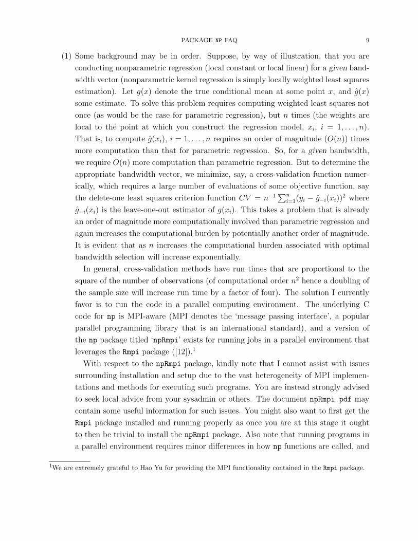
(1) Some background may be in order. Suppose, by way of illustration, that you are
conducting nonparametric regression (local constant or local linear) for a given band-
width vector (nonparametric kernel regression is simply locally weighted least squares
estimation). Let g(x) denote the true conditional mean at some point x, and g(x)
some estimate. To solve this problem requires computing weighted least squares not
once (as would be the case for parametric regression), but n times (the weights are
local to the point at which you construct the regression model, xi, i = 1, . . . , n).
That is, to compute g(xi), i = 1, . . . , n requires an order of magnitude (O(n)) times
more computation than that for parametric regression. So, for a given bandwidth,
we require O(n) more computation than parametric regression. But to determine the
appropriate bandwidth vector, we minimize, say, a cross-validation function numer-
ically, which requires a large number of evaluations of some objective function, say
the delete-one least squares criterion function CV = n−1∑n
i=1(yi − g−i(xi))2 where
g−i(xi) is the leave-one-out estimator of g(xi). This takes a problem that is already
an order of magnitude more computationally involved than parametric regression and
again increases the computational burden by potentially another order of magnitude.
It is evident that as n increases the computational burden associated with optimal
bandwidth selection will increase exponentially.
In general, cross-validation methods have run times that are proportional to the
square of the number of observations (of computational order n2 hence a doubling of
the sample size will increase run time by a factor of four). The solution I currently
favor is to run the code in a parallel computing environment. The underlying C
code for np is MPI-aware (MPI denotes the ‘message passing interface’, a popular
parallel programming library that is an international standard), and a version of
the np package titled ‘npRmpi’ exists for running jobs in a parallel environment that
leverages the Rmpi package ([12]).1
With respect to the npRmpi package, kindly note that I cannot assist with issues
surrounding installation and setup due to the vast heterogeneity of MPI implemen-
tations and methods for executing such programs. You are instead strongly advised
to seek local advice from your sysadmin or others. The document npRmpi.pdf may
contain some useful information for such issues. You might also want to first get the
Rmpi package installed and running properly as once you are at this stage it ought
to then be trivial to install the npRmpi package. Also note that running programs in
a parallel environment requires minor differences in how np functions are called, and
1We are extremely grateful to Hao Yu for providing the MPI functionality contained in the Rmpi package.

10 JEFFREY S. RACINE
you would be wise to examine the examples in the demo directory (download and
unpack the source code and look in this directory) and the overview file npRmpi.pdf
in the inst/doc/ directory of the npRmpi package you downloaded and unpacked.
(2) Alternatively, you can use the method outlined in Racine (1993) [9]. The method is
based on the fact that the unknown constant cj (the ‘scale factor’) in the formula
cjσjn−1/(2p+r) is independent of the sample size, so one can conduct bandwidth se-
lection on random subsets and do this for a large number of subsets then take the
mean/median over these subsets and feed the scale factor into the final routine for
the entire sample. Below you will find simple R code that replicates the method using
numerical search and resampling without replacement rather than the grid method
outlined in [9] (both have equivalent properties but this is perhaps simpler to imple-
ment using the np package).
## Regression example
## Generate a moderately large data set
set.seed(12345)
n <- 100000
x1 <- runif(n)
x2 <- runif(n)
y <- 1 + x1 + sin(pi*x2) + rnorm(n,sd=.1)
## Set the number of resamples and the subsample size
num.res <- 50
n.sub <- 250
## Create a storage matrix
bw.mat <- matrix(NA,nrow=num.res,ncol=2)
## Get the scale factors for resamples from the full sample of size n.sub
options(np.messages=FALSE)
for(i in 1:num.res) {
cat(paste(" Replication", i, "of", num.res, "...\r"))
bw.mat[i,] <- npregbw(y~x1+x2,regtype="ll",

PACKAGE NP FAQ 11
subset=sample(n,n.sub))$sfactor$x
}
## A function to compute the median of the columns of a matrix
colMedians <- function(data) {
colmed <- numeric(ncol(data))
for(i in 1:ncol(data)) {
colmed[i] <- median(data[,i])
}
return(colmed)
}
## Take the median scale factors
bw <- colMedians(bw.mat)
## The final model for the full dataset
model.res <- npreg(y~x1+x2,bws=bw,regtype="ll",bwscaling=TRUE)
## Hat tip to Yoshi Fujiwara <[email protected]> for this
## nice example
n <- 100000
library(MASS)
rho <- 0.25
Sigma <- matrix(c(1,rho,rho,1),2,2)
mydat <- mvrnorm(n=n, rep(0, 2), Sigma)
x <- mydat[,1]
y <- mydat[,2]
rm(mydat)
num.res <- 100
n.sub <- 100
bw.mat <- matrix(NA,nrow=num.res,ncol=2)
options(np.messages=FALSE)
for(i in 1:num.res) {
bw <- npcdensbw(y ~ x,subset=sample(n,n.sub))
bw.mat[i,] <- c(bw$sfactor$y,bw$sfactor$x)

12 JEFFREY S. RACINE
}
colMedians <- function(data) {
colmed <- numeric(ncol(data))
for(i in 1:ncol(data)) {
colmed[i] <- median(data[,i])
}
return(colmed)
}
bw <- colMedians(bw.mat)
bw <- npcdensbw(y ~ x, bws=bw, bwscaling=TRUE, bandwidth.compute=FALSE)
summary(bw)
plot(bw,xtrim=.01)
(3) Barring this, you can set the search tolerances to be a bit less terse (at the expense of
potential accuracy, i.e., becoming trapped in local minima) by setting, say, tol=0.1
and ftol=0.1 in the respective bandwidth routine (see the docs for examples). Also,
you can set nmulti=1 which overrides the number of times the search procedure
restarts from different random starting values (the default is to restart k times where
k is the number of variables). Be warned, however, that this is definitely not recom-
mended and should be avoided at all costs for all but the most casual examination of
a relationship. One ought to use multistarting for any final results and never override
default search tolerances unless increasing multistarts beyond the default. Results
based upon exhaustive search often differ dramatically from that based on limited
search achieved by overriding default search tolerances.(4) For those who like to tinker and who work on a *NIX system with the gcc compiler
suite, you can change the default compiler switches used for building R packageswhich may generate some modest improvements in run time. The default compilerswitches are
-g -O2
and are set in the R-*.*.*/etc/Makeconf file (where *.*.* refers to your R versionnumber, e.g. R-2.10.1). You can edit this file and change these defaults to
-O3 -ffast-math -fexpensive-optimizations -fomit-frame-pointer
then reinstall the np package and you may experience some improvements in run
time. Note that the -g flag turns on production of debugging information which can
involve some overhead, so we are disabling this feature. This is not a feature used by
the typical applied researcher but if you envision requiring this it is clearly trivial to

PACKAGE NP FAQ 13
re-enable debugging. I typically experience in the neighborhood of a 0-5% reduction
in run time for data-driven bandwidth selection on a variety of systems depending
on the method being used, though mileage will of course vary.
(5) Finally, I have recently been working on extending regression splines (as opposed to
smoothing splines2) to admit categorical predictors (see references for papers with
Yang and Ma in the crs package). Because regression splines involve simple (i.e.,
‘global’ as opposed to local) least-squares fits, they scale much better with respect
to the sample size so for large sample sizes you may wish to instead consider this
approach (kindly see my webpage for further details). You can run cross-validation
with hundreds of thousands of observations on a decent desktop in far less time than
that required for cross-validated kernel estimates. Be forewarned, however, that the
presence of categorical predictors can lead to increased execution time unless the
option kernel=FALSE is invoked (the default is to use local kernel weighting in the
presence of categorical predictors).
2.11. Is there a way to figure out roughly how long cross-validation will take on a
large sample? Certainly. You can run cross-validation on subsets of your data of increasing
size and time each run, then estimate a double-log model of sample size on run time (run time
can be approximated by a linear log-log model) and then use this to predict approximate
run-time. The following example demonstrates this for a simple model, but you can modify
it trivially for your data. Note that the larger is n.max the more accurate it will likely be.
Note that we presume your data is in no particular order (if it is, you perhaps ought to
shuffle it first). We plot the log-log model fit and prediction along with that expressed in
hours.
## Set the upper bound (n.max > 100) for the sub-samples on which you
## will run cross-validation (perhaps n.max = 1000 (or 2000) ought to
## suffice). For your application, n will be your sample size
n <- 2000
n.max <- 1000
x <- runif(n)
y <- 1 + x + rnorm(n)
2Unlike regression splines, a smoothing spline places a knot at each data point and penalizes the fit for lackof smoothness as defined by the second derivative (typically cubic splines are used). When the penalty iszero this produces a function that interpolates the data points. When the penalty is infinite, this deliversthe linear OLS fit to the data.

14 JEFFREY S. RACINE
n.seq <- seq(100,n.max,by=100)
time.seq <- numeric(length(n.seq))
for(i in 1:length(n.seq)) {
time.seq[i] <- system.time(npregbw(y~x,subset=seq(1:n.seq[i])))[3]
}
## Now fit a double-log model and generate/plot actual values plus
## prediction for n (i.e., approximate run time in hours)
log.time <- log(time.seq)
log.n <- log(n.seq)
model <- lm(log.time~log.n)
n.seq.aug <- c(n.seq,n)
time.fcst <- exp(predict(model,newdata=data.frame(log.n=log(n.seq.aug))))
par(mfrow=c(2,1))
plot(log(n.seq.aug),log(time.fcst),type="b",
xlab="log(Sample Size)",
ylab="log(Run Time)",
main="Approximate Run Time (log seconds)")
plot(n.seq.aug,time.fcst/3600,type="b",
xlab="Sample Size (n)",
ylab="Hours",
main="Approximate Run Time (hours)",
sub=paste("Predicted run time for n =", n, "observations:",
signif(time.fcst[length(time.fcst)]/3600, digits=2),
"hours"))
2.12. Where can I get some examples of R code for the np package in addition
to the examples in the help files? Start R then type demo(package="np") and you will
be presented with a list of demos for constrained estimation, inference, and so forth. To run
one of these demos type, for example, demo(npregiv) (note that you must first install the
rgl package to run this particular demo).
To find the location of a demo type system.file("demo","npregiv.R",package="np")
for example, then you can take the source code for this demo and modify it for your particular
application.

PACKAGE NP FAQ 15
You can also find examples and illustrations at the ‘Gallery’ located at http://socserv.
mcmaster.ca/racinej/Gallery/Home.html.
2.13. I need to apply a boundary correction for a univariate density estimate -
how can I do this? As of version 0.60.5, you can use either npuniden.boundary (boundary
kernel functions) or npuniden.reflect (data reflection).
2.14. I notice your density estimator supports manual bandwidths, the normal-
reference rule-of-thumb, likelihood cross-validation and least squares cross-
validation, but not plug-in rules. How can I use various plug-in rules for es-
timating a univariate density? For the univariate case this is straightforward as the
default R installation supports a variety of univariate plug-in bandwidths (see ?bw.nrd for
details). For example, bs.SJ computes the bandwidths outlined in
Sheather, S. J. and Jones, M. C. (1991) A reliable data-based
bandwidth selection method for kernel density estimation.
_Journal of the Royal Statistical Society series B_, *53*,
683-690.
Incorporating these univariate plug-in bandwidth selectors into the univariate density es-
timation routines in np is straightforward as the following code snippet demonstrates. They
will certainly be faster than the likelihood and least-squares cross-validation approaches.
Also, you may not wish the density estimate for all sample realizations, but rather for a
shorter grid. The following example demonstrates both and is closer in spirit to the den-
sity() function in base R.
x <- rnorm(10000)
xeval <- seq(min(x),max(x),length=100)
f <- npudens(tdat=x,edat=xeval,bws=bw.SJ(x))
You might even be tempted to use these in the multivariate case via bws=c(bw.SJ(x1),bw.SJ(x2),...)
though these would be optimal for univariate densities and most certainly not for a multi-
variate density. However, for exploratory purposes these may be of interest to some users.
2.15. I wrote a program using np and it does not work as I expected. . . There exist
a rather extensive set of examples contained in the docs. You can run these examples by
typing example("npfunctionname") where npfunctionname is, say, w, as in example("w").3
These examples all pass quality control and produce the expected results, so first see whether
3For a listing of all routines in the np package type: library(help="np").
16 JEFFREY S. RACINE
your problem fits into an existing example, and if not, carefully follow the examples listed
in a given function for syntax issues etc.
If you are convinced that the problem lies with np (there certainly will be undiscovered
‘features’, i.e., bugs), then kindly send me your code and data so that I can replicate and
help resolve the issue.
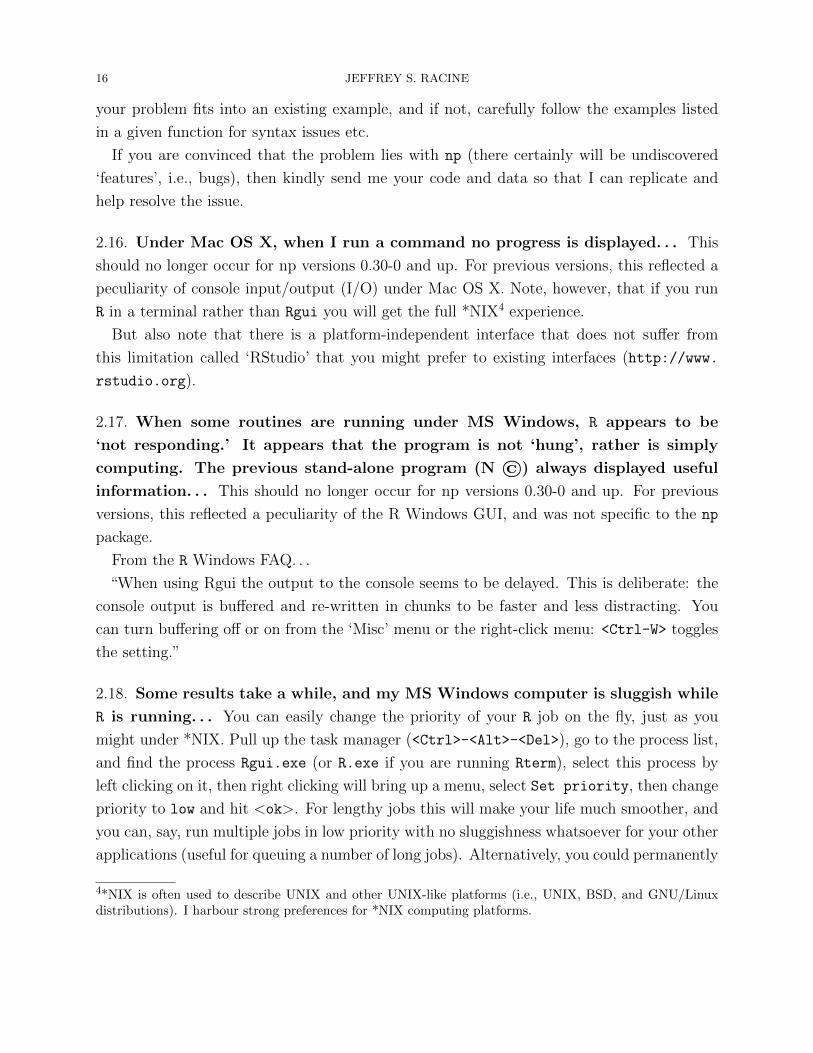
2.16. Under Mac OS X, when I run a command no progress is displayed. . . This
should no longer occur for np versions 0.30-0 and up. For previous versions, this reflected a
peculiarity of console input/output (I/O) under Mac OS X. Note, however, that if you run
R in a terminal rather than Rgui you will get the full *NIX4 experience.
But also note that there is a platform-independent interface that does not suffer from
this limitation called ‘RStudio’ that you might prefer to existing interfaces (http://www.
rstudio.org).
2.17. When some routines are running under MS Windows, R appears to be
‘not responding.’ It appears that the program is not ‘hung’, rather is simply
computing. The previous stand-alone program (N ©) always displayed useful
information. . . This should no longer occur for np versions 0.30-0 and up. For previous
versions, this reflected a peculiarity of the R Windows GUI, and was not specific to the np
package.
From the R Windows FAQ. . .
“When using Rgui the output to the console seems to be delayed. This is deliberate: the
console output is buffered and re-written in chunks to be faster and less distracting. You
can turn buffering off or on from the ‘Misc’ menu or the right-click menu: <Ctrl-W> toggles
the setting.”
2.18. Some results take a while, and my MS Windows computer is sluggish while
R is running. . . You can easily change the priority of your R job on the fly, just as you
might under *NIX. Pull up the task manager (<Ctrl>-<Alt>-<Del>), go to the process list,
and find the process Rgui.exe (or R.exe if you are running Rterm), select this process by
left clicking on it, then right clicking will bring up a menu, select Set priority, then change
priority to low and hit <ok>. For lengthy jobs this will make your life much smoother, and
you can, say, run multiple jobs in low priority with no sluggishness whatsoever for your other
applications (useful for queuing a number of long jobs). Alternatively, you could permanently
4*NIX is often used to describe UNIX and other UNIX-like platforms (i.e., UNIX, BSD, and GNU/Linuxdistributions). I harbour strong preferences for *NIX computing platforms.

PACKAGE NP FAQ 17
change the default priority of R under MS Windows by modifying the properties of your R
desktop icon.
2.19. A variable must be cast as, say, a factor in order for np to recognize this as an
unordered factor. How can I determine whether my data is already cast as a fac-
tor? Use the class() function. For example, define x <- factor(c("male","female")),
then type class(x).
2.20. When I use plot() (npplot()) existing graphics windows are overwritten.
How can I display multiple graphics plots in separate graphics windows so that
I can see results from previous runs and compare that to my new run? Use the
dev.new() command in between each call to plot(). This will leave the existing graphics
window open and start a new one. The command dev.list() will list all graphics windows,
and the command dev.set(integer.foo) will allow you to switch from one to another and
overwrite existing graphics windows should you so choose.
Alternately, you can use RStudio (http://www.rstudio.org) where the plot window is
such that previous plots can be recalled on the fly, resized, saved in various formats etc.
2.21. Sometimes plot() fails to use my variable names. . . This should not occur
unless you are using the data frame method and not naming your variables (e.g., you are
doing something like data.frame(ordered(year))). To correct this, name your variables in the
respective data frame, as in
data <- data.frame(year=ordered(year),gdp)
so that the ordered factor appears as ‘year’ and not ‘ordered.year’
2.22. Sometimes plot() appends my variable names with .ordered or .factor. . .
See also 2.21 above.
2.23. I specify a variable as factor() or ordered() in a data frame, then call
this when I conduct bandwidth selection. However, when I try to plot the
resulting object, it complains with the following message: Error in eval(expr,
envir, enclos) : object "variable" not found...
This arises because plot() (npplot()) tries to retrieve the variable from the environment
but you have changed the definition when you called the bandwidth selection routine (e.g.,
npregbw(y~x,data=dataframe)).
To correct this, simply call plot() with the argument data=dataframe where dataframe
is the name of your data frame.

18 JEFFREY S. RACINE
2.24. My np code produces errors when I attempt to run it. . . First, it is good
practice to name all arguments (see the docs for examples) as in npregbw(formula=y~x)
(i.e., explicitly call formula for functions that use named formulas). This will help the code
return a potentially helpful error message.
Next, follow the examples listed at the end of each function help page closely (i.e., ?npreg
then scroll down to Examples:). See also 2.15 above.
2.25. I have (numeric) 0/1 dummy variable regressors in my parametric model.
Can I just pass them to the np functions as I would in a parametric setting? In
general, definitely not – you need to correctly classify each variable as type factor and treat
it as one variable only. By way of example, suppose in your data you have created dummy
variables for year, for example, dummy06 which equals 1 for 2006, 0 otherwise, dummy07
which equals 1 for 2007, 0 otherwise etc. We create these by habit for parametric models.
But, the underlying variable is simply year, which equals 2006, 2007, and so forth.
In np (and R in general), you get to economize by just telling the function that the variable
‘year’ is ordered, as in ordered(year), where year is a vector containing elements 2006, 2007
etc. Of course, seasoned R users would appreciate that this is in fact the simple way to do
it with a parametric model as well.
You would never, therefore, just pass dummy variables to an np function as you would for
linear parametric models. The only exception is where you have only one 0/1 dummy for
one variable, say ‘sex’, and in this case you still would have to enter this as factor(sex)
so that the np function recognizes this as a factor (otherwise it would treat it as continuous
and use a kernel function that is inappropriate for a factor).
2.26. I have a categorical variable, ignored the advice in items 2.19 and 2.25, and
R terminates with the following error.
** Fatal Error in routine kernel_bandwidth() ** variable 0 appears to be constant!
** Program terminated abnormally!
Presuming your variable is not in fact a constant (i.e., is not in fact a ‘variable’), this can
only occur in the case where a variable is ‘pathological’ in that it has IQR=0 but std>0 (see
the section titled ‘Changes from Version 0.30-1 to 0.30-2 [19-Apr-2009]’ for further details).
This should no longer occur for np versions 0.30-2 and up.
2.27. Rgui appears to crash. There must be a bug in the program. Try running
your code using the terminal (i.e., Rterm in Windows or R in a Mac OS X terminal) and see
whether you get the message in item 2.26.

PACKAGE NP FAQ 19
2.28. Can I skip creating a bandwidth object and enter a bandwidth directly?Certainly, though I would advise doing so for exploratory data analysis only. For example,attach a dataset via
data(cps71)
attach(cps71)
then enter, say,
plot(age,logwage,main="Manual Bandwidth Example")
lines(age,fitted(npreg(logwage~age,bws=1)),col="blue",lty=1)
lines(age,fitted(npreg(logwage~age,bws=2)),col="red",lty=2)
lines(age,fitted(npreg(logwage~age,bws=3)),col="green",lty=3)
legend(20,15,
c("h=1","h=2","h=3"),
col=c("blue","red","green"),
lty=c(1,2,3))
to plot the local constant estimator with bandwidths of 1, 2, and 3 years. Note that the
age variable is already sorted in this dataset. If your data is not sorted you will need to do
so prior to plotting so that your lines command works properly. Or see 2.29 below for a
multivariate example.
2.29. When I estimate my gradients and there are two or more covariates and
then extract them with the gradients() function, they are not ‘smooth’, though
if I plot a model with the gradients=TRUE option, they are. The gradients()
function must be broken. . . The function plot() (npplot()) plots ‘partial’ means and
gradients. In other words, it plots x1 versus g(x1, x2) for the partial mean, where x2 is, say,
the median/modal value of x2. It also plots x1 versus ∂g(x1, x2)/∂x1 for the gradient. Note
that we are controlling for the values of the other covariate(s). This is in effect what people
expect when they play with linear parametric models of the form y = β0 + β1x1 + β2x2 + ε
since, given the additive nature of the model, ∂y/∂x1 = β1 (i.e., does not vary with x2).
The example below shows how you could manually generate the partial gradients (and
means) for your data where the sample realizations form the evaluation data for x1 (unlike
npplot() which uses an evenly spaced grid). Note we use the function uocquantile() to
generate a vector that holds x2 constant at is median/modal value (i.e., the 0.5 quantile)
in the evaluation data. The function uocquantile() can compute quantiles for ordered,
unordered, and continuous data (see ?uocquantile for details).
n <- 100

20 JEFFREY S. RACINE
x1 <- runif(n)
x2 <- runif(n)
y <- x1^2+x2^2 + rnorm(n,sd=.1)
data.train <- data.frame(x1,x2,y)
bw <- npregbw(y~x1+x2,
data=data.train,
regtype="ll",
bwmethod="cv.aic")
data.eval <- data.frame(x1 = sort(x1),
x2 = rep(uocquantile(x2,.5),n))
model <- npreg(bws=bw,
data=data.train,
newdata=data.eval,
gradients=TRUE)
plot(data.eval[,1],model$grad[,1],xlab="X1",ylab="Gradient",type="l")
Note that this uses the sorted sample realizations for x1 which is perfectly acceptable. Ifyou want to mimic plot() exactly you will see that by default plot uses a grid of equallyspaced values of length neval=50 as per below. Both are perfectly acceptable and the pointis they control for the level of the non-axis variables.
data.eval <- data.frame(x1 = seq(min(x1),max(x1),length=50),
x2 = rep(uocquantile(x2,.5),50))
2.30. I use plot() (npplot()) to plot, say, a density and the resulting plot looks
like an inverted density rather than a density. . . This can occur when the data-
driven bandwidth is dramatically undersmoothed. Data-driven (i.e., automatic) bandwidth
selection procedures are not guaranteed always to produce good results due to perhaps the
presence of outliers or the rounding/discretization of continuous data, among others. By
default, npplot() takes the two extremes of the data (minimum, maximum i.e., actual data
points) then creates an equally spaced grid of evaluation data (i.e., not actual data points in
general) and computes the density for these points. Since the bandwidth is extremely small,
the density estimate at these evaluation points is correctly zero, while those for the sample
realizations (in this case only two, the min and max) are non-zero, hence we get two peaks
at the edges of the plot and a flat bowl equal to zero everywhere else.
This can also happen when your data is heavily discretized and you treat it as continuous.
In such cases, treating the data as ordered may result in more sensible estimates.

PACKAGE NP FAQ 21
2.31. Can npksum() compute analytical derivatives with respect to a continuous
variable? As of version 0.20-0 and up, yes it can, using the operator = "derivative"
argument, which is put to its paces in the following code snippet (this supports multiple
arguments including "integral" and "convolution" in addition to "normal", the default).
Z <- seq(-2.23,2.23,length=100)
Zc <- seq(-4.47,4.47,length=100)
par(mfrow=c(2,2))
plot(Z,main="Kernel",ylab="K()",npksum(txdat=0,exdat=Z,bws=1,
ckertype="epanechnikov",ckerorder=2,operator="normal")$ksum,
col="blue",type="l")
plot(Z,main="Kernel Derivative",ylab="K()",npksum(txdat=0,exdat=Z,bws=1,
ckertype="epanechnikov",ckerorder=2,operator="derivative")$ksum,
col="blue",type="l")
plot(Z,main="Kernel Integral",ylab="K()",npksum(txdat=0,exdat=Z,bws=1,
ckertype="epanechnikov",ckerorder=2,operator="integral")$ksum,
col="blue",type="l")
plot(Zc,main="Kernel Convolution",ylab="K()",npksum(txdat=0,exdat=Zc,bws=1,
ckertype="epanechnikov",ckerorder=2,operator="convolution")$ksum,
col="blue",type="l")
An alternative to computing analytical derivatives is to compute them numerically using
finite-differences. One simply computes the kernel sum evaluating the sum with variable j
set at xj−hj/2 and calls this, say, ksumj1, then again set at xj +hj/2 and call this ksumj2,
then compute ∇ = (ksumj2 − ksumj1)/hj. This method has been used for both theoretical
and applied work and produces consistent estimates of the derivatives, as of course do the
analytical derivatives, providing that h → 0 as n → ∞ (which will not be the case in some
settings, i.e., in the presence of irrelevant covariates and so forth). The following example
provides a simple demonstration. See 2.29 above for multivariate partial regression when
using this method.
## In this example we consider the local constant estimator computed
## using npksum, and then use npksum to compute numerical derivatives
## using finite-difference methods, then finally compare them with the
## analytical ones.

22 JEFFREY S. RACINE
data(cps71)
attach(cps71)
## Grab the cross-validated bandwidth
bw <- npregbw(logwage~age)
h <- bw$bw[1]
## Evaluate the local constant regression at x-h/2, x+h/2...
ksum.1 <- npksum(txdat=age, exdat=age-h/2,tydat=logwage,bws=bw)$ksum/
npksum(txdat=age,exdat=age-h/2,bws=bw)$ksum
ksum.2 <- npksum(txdat=age, exdat=age+h/2,tydat=logwage,bws=bw)$ksum/
npksum(txdat=age,exdat=age+h/2,bws=bw)$ksum
## Compute the numerical gradient...
grad.numerical <- (ksum.2-ksum.1)/h
## Compare with the analytical gradient...
grad.analytical <- gradients(npreg(bws=bw,gradient=TRUE))
## Plot the resulting estimates...
plot(age,grad.numerical,type="l",col="blue",lty=1,ylab="gradient")
lines(age,grad.analytical,type="l",col="red",lty=2)
legend(20,-0.05,c("Numerical","Analytic"),col=c("blue","red"),lty=c(1,2))
2.32. Can I use the npcmstest() function that implements the consistent test for
correct specification of parametric regression models as described in Hsiao, Li, &
Racine (2007) [6] to test for correct specification of the semiparametric partially
linear model? As Brennan Thompson points out, yes, you can.
To test a parametric linear specification against a semiparametric partially linear alterna-
tive, i.e.,
H0 : y = X ′β + Z ′γ + u
H1 : y = X ′β + g(Z) + u,
you could use npcmstest() as follows:
lmodel <- lm(y~X+Z,y=TRUE,x=TRUE)

PACKAGE NP FAQ 23
uhat <- resid(lmodel)
npcmstest(xdat=Z,ydat=uhat,model=lmodel)
A slightly better way (as discussed in Li & Wang (1998) [8]) would be to use a ‘mixed’
residual, i.e., ui = yi −X ′iβ − Z ′iγ in the test, where β is the semiparametric estimator of β
(based on the semiparametric partially linear model), and γ is the OLS estimator of γ based
on the linear model. This could lead to potential power gains due to the improved efficiency
of β under the alternative.
2.33. I am using npcmstest() on a glm() object (the document says glm() objects
are supported and I am estimating a Logit model) but it returns an error saying.
Error in eval(expr, envir, enclos) : y values must be 0 <= y <= 1.
npcmstest() supports conditional mean models with continuous outcomes (glm() objects
are supported so that models that are nonlinear in parameters can be estimated). The test
is based on residual bootstrapping to generate resamples for Y . In particular, a resample for
the residual vector (ε∗) is added to the models’ fit (i.e., Y ∗ = Y + ε∗) to generate a resample
under the null. This excludes binary outcome models and the like because you would have
generated a resample for Y that no longer contains zeros and ones, hence the error message.
Note that npcmstest supports regression objects generated by lm and uses features specific
to objects of type lm hence if you attempt to pass objects of a different type the function
cannot be expected to work.
2.34. I want to plot the kernel function itself. How can I do this? Use the npksum()function and switch the evaluation and training roles as in the following example that plotsthe 2nd, 4th, 6th and 8th order Epanechnikov kernels.
Z <- seq(-sqrt(5),sqrt(5),length=100)
par(mfrow=c(2,2))
plot(Z,ylab="kernel",npksum(txdat=0,exdat=Z,bws=1,ckertype="epanechnikov",
ckerorder=2)$ksum,type="l",main="Epanechnikov [order = 2]")
plot(Z,ylab="kernel",npksum(txdat=0,exdat=Z,bws=1,ckertype="epanechnikov",
ckerorder=4)$ksum,type="l",main="Epanechnikov [order = 4]")
plot(Z,ylab="kernel",npksum(txdat=0,exdat=Z,bws=1,ckertype="epanechnikov",
ckerorder=6)$ksum,type="l",main="Epanechnikov [order = 6]")
plot(Z,ylab="kernel",npksum(txdat=0,exdat=Z,bws=1,ckertype="epanechnikov",
ckerorder=8)$ksum,type="l",main="Epanechnikov [order = 8]")
2.35. In version 0.20-0 and up I can ‘combine’ steps such as bandwidth selection
and estimation. But when I do summary(model) I don’t get the same summary
that I would get from, say, summary(bw) and then summary(model). How do I get
bandwidth object summaries when combining steps? Don’t worry, the bandwidth

24 JEFFREY S. RACINE
object exists when you do the combined steps and is easily accessed via summary(model$bws)
or extracted via bw <- model$bws where model is the name of your model.
2.36. I estimated a semiparametric index model via model <- npindex(y~x1+x2)
but se(model) returns NULL. .
Perhaps you want vcov(model) instead (i.e., the asymptotic variance-covariance matrix)?
This is supported as of version 0.40-1 provided that you set gradients=TRUE as the following
snippet demonstrates:
set.seed(42)
n <- 250
x1 <- runif(n, min=-1, max=1)
x2 <- runif(n, min=-1, max=1)
y <- ifelse(x1 + x2 + rnorm(n) > 0, 1, 0)
## Note that the first element of the vector beta is normalized to one
## for identification purposes hence the first row and column of the
## covariance matrix will contain zeros.
model <- npindex(y~x1+x2, method="kleinspady", gradients=TRUE)
vcov(model)
Z <- coef(model)[-1]/sqrt(diag(vcov(model)))[-1]
Z
Note that, alternatively, you can get robust bootstrapped standard errors for the esti-
mated model and gradients by adding the argument errors=TRUE to your call to npindex
so that se(model) returns the vector of standard errors for the estimated conditional mean
where model is the name of your model. Note that model$merr will contain the standard
errors returned by se(model) while model$gerr will return the matrix of standard errors for
the gradients provided you have set gradients=TRUE (furthermore, model$mean.grad and
model$mean.gerr will give the average derivative and its bootstrapped standard errors). See
the documentation of npindex for further details. The following code snippet demonstrates
how one could do this for a simulated dataset.
n <- 100
x1 <- runif(n, min=-1, max=1)
x2 <- runif(n, min=-1, max=1)
y <- x1 - x2 + rnorm(n)
bw <- npindexbw(formula=y~x1+x2)

PACKAGE NP FAQ 25
model <- npindex(bws=bw,errors=TRUE,gradients=TRUE)
se.mean <- model$merr
se.grad <- model$gerr
2.37. How do I interpret gradients from the conditional density estimator? If you
plot a conditional density f(y|x) when x is a scalar, with gradients, by default you will get
the following:
(1) A plot of ∂f(y = median|x)/∂x (admittedly not the most useful plot). (If y is discrete
the only difference is that you get a plot of ∂f(y = (unconditional) mode|x)/∂x).
(2) A plot of ∂f(y|x = median)/∂x.
If x is multivariate (for example, 2D) you get:
(1) A plot of ∂f(y = median|x1, x2 = median)/∂x1
(2) A plot of ∂f(y = median|x1, x2 = median)/∂x2
(3) A plot of ∂f(y = median|x1 = median, x2)/∂x1
(4) A plot of ∂f(y = median|x1 = median, x2)/∂x2
(5) A plot of ∂f(y|x1 = median, x2 = median)/∂x1
(6) A plot of ∂f(y|x1 = median, x2 = median)/∂x2
2.38. When I run R in batch mode via R CMD BATCH filename.R unwanted status
messages (e.g., “‘Multistart 1 of 10”’) crowd out desired output. How can I
turn off these unwanted status messages? After loading the np library add the line
options(np.messages=FALSE) and all such messages will be disabled.
2.39. I am getting an ‘unable to allocate...’ message after repeatedly interrupting
large jobs. Repeated interruption of large jobs can reduce available memory under R. This
occurs because memory is allocated dynamically, and memory that has been allocated is not
freed when you interrupt the job (the routine will clean up after itself only if it is allowed to
complete all computations - when you interrupt you never reach the point in the code where
the memory is freed). If this becomes an issue simply restart R (i.e., exit then run a fresh R
session).
2.40. I have a large number of variables, and when using the formula interface
I get an error message stating ‘invoked with improper formula’. I have double
checked and everything looks fine. Furthermore, it works fine with the data
frame interface. The issue is that converting formulas into character strings in R appears

26 JEFFREY S. RACINE
to be limited to 500 characters. We are not aware of a simple workaround so we simply
advise that you use the data frame interface when this occurs.
2.41. How can I estimate additive semiparametric models? Generalized additive
semiparametric models (see Hastie and Tibshirani (1990) [4]) are implemented in the gam
package (though they do not support categorical variables). The gam package function
gam() (the mgcv package also contains a similar function by the same name) uses iteratively
reweighted least squares and either smoothing splines (s(·)) or local polynomial regression
fitting (‘loess’, lo(·), with default manual ‘span’ of 0.75, the parameter which controls the
degree of smoothing). The following code snippet demonstrates the capabilities of the gam()
function via the wage1 dataset included in the np packages using three numeric regressors.
library(gam)
data(wage1)
attach(wage1)
model.gam <- gam(lwage~s(educ)+s(exper)+s(tenure))
par(mfrow=c(2,2))
plot(model.gam,se=T)
detach(wage1)
The mgcv package also has an implementation of generalized additive models via the
identical function name, gam(). The biggest difference is that this uses generalized cross
validation to select the ‘span’ (rather than manually) hence the degree of smoothing becomes
part of the method (as is the case for all functions in the np package). The following code
snippet demonstrates the mgcv implementation of the gam() function.
library(mgcv)
data(wage1)
attach(wage1)
model.gam <- gam(lwage~s(educ)+s(exper)+s(tenure))
par(mfrow=c(2,2))
plot(model.gam,se=T)
detach(wage1)
2.42. I am using npRmpi and am getting an error message involving dlopen(). One
of the most common problems experienced by users attempting to install and run MPI-aware
programs is to first correctly identify the location of libraries and headers for the local MPI
installation so that installation can proceed.

PACKAGE NP FAQ 27
By way of illustration, the following environment variables need to be set for the MacPorts
version of OpenMPI (www.macports.org) running on Mac OS X 10.8.3 (the environment
commands listed below are for those using the ‘bash’ shell):
export LD_LIBRARY_PATH=/opt/local/lib
export RMPI_LIB_PATH=/opt/local/lib
export RMPI_TYPE=OPENMPI
export RMPI_INCLUDE=/opt/local/include/openmpi
launchctl setenv LD_LIBRARY_PATH $LD_LIBRARY_PATH
launchctl setenv RMPI_LIB_PATH $RMPI_LIB_PATH
launchctl setenv RMPI_TYPE $RMPI_TYPE
launchctl setenv RMPI_INCLUDE $RMPI_INCLUDE
Once set, R (and optionally RStudio) ought to function as expected. However, problems
encountered during this phase are best resolved by someone with familiarity of the local
installation.
2.43. I am using the npRmpi package but when I launch one of the demo parallel
jobs I get the error Error: could not find function "mpi.bcast.cmd". When your
demo program stops at the following point in your file
> mpi.bcast.cmd(np.mpi.initialize(),
+ caller.execute=TRUE)
Error: could not find function "mpi.bcast.cmd"
this likely means that either you have failed to place the .Rprofile file in the current or root
directory as directed, or the .Rprofile initialization code is not being loaded as expected.
(1) Make sure a copy of the initialization file Rprofile exists in your working or root
directory and is named .Rprofile
(2) Make sure you did not run R with either the -no-init-file or -vanilla option (this
combines a number of options including -no-init-file which will disable reading
of .Rprofile)
2.44. I have estimated a partially linear model and want to extract the gradi-
ent/fitted values of the nonparametric component. People use partially linear models
because they focus on the parametric component and treat the nonparametric component
as a nuisance. In fact, the partially linear model is estimated by carefully getting rid of the
nonparametric component g(Z) prior to estimation, and then estimating a set of conditional
moments nonparametrically.

28 JEFFREY S. RACINE
However, suppose after getting rid of this nonparametric nuisance component we then
wished to construct a consistent estimator of g(Z), the nonparametric component for a
partially linear model y = Xβ + g(Z) + u. We might proceed as follows.
library(np)
set.seed(42)
n <- 250
x1 <- rnorm(n)
x2 <- rbinom(n, 1, .5)
z1 <- rbinom(n, 1, .5)
z2 <- rnorm(n)
y <- 1 + x1 + x2 + z1 + sin(z2) + rnorm(n)
## First, construct the partially linear model using local linear
## regression.
model <- npplreg(y~x1+factor(x2)|factor(z1)+z2,regtype="ll")
## Next, subtract the fitted parametric component from y so that we
## have y-xbetahat. Since we can have factors we need to create the
## `model matrix' but make sure we don't keep the intercept generated
## by model.matrix hence the [,-1]. This gives us the numeric matrix X
## which we multiply by the coefficient vector to obtain xbetahat which
## we can subtract from y.
y.sub <- y-model.matrix(~x1+factor(x2))[,-1]%*%coef(model)
## Finally, regress this on the nonparametric components Z using npreg.
model.sub <- npreg(y.sub~factor(z1)+z2,regtype="ll",gradients=TRUE)
## Now we can obtain derivatives etc. However, note that this is the

PACKAGE NP FAQ 29
## model containing the transformed y with respect to the nonparametric
## components. We can use gradients(model.sub) etc. or plot them and
## so forth.
plot(model.sub,gradients=TRUE)
2.45. The R function ‘lag()’ does not work as I expect it to. How can I create
the lth lag of a numeric variable in R to be fed to functions in the np package?
As of version 0.60-2, time series objects are supported. However, if you prefer you can use
the function ts.intersect, which can exploit R’s lag function but return a suitable data
frame, as per the following illustration:
data(lynx)
loglynx <- log(lynx)
lynxdata <- ts.intersect(loglynx,
loglynxlag1=lag(loglynx,-1),
dframe=TRUE)
model <- npregbw(loglynx~loglynxlag1,
data=lynxdata)
plot(model)
Note that in order for the above to work, the common argument fed to ts.intersect must
be a ts object, so first cast it as such if it is not already (log(lynx) is a ts object since
lynx was itself a ts object).
Or, you can use the embed function to accomplish this task. Here is a simple function that
might work more along the lines that you expect. By default we ‘pad’ the vector with NAs
but you can switch this to FALSE if you prefer. The function will return a vector of the same
length as the original vector with NA’s padded for the missing values.
lag.numeric <- function(x,l=1,pad.NA=TRUE) {
if(!is.numeric(x)) stop("x must be numeric")
if(l < 1) stop("l (lag) must be a positive integer")
if(pad.NA) x <- c(rep(NA,l),x)
return(embed(x,l+1)[,l+1])
}
x <- 1:10
x.lag.1 <- lag.numeric(x,1)

30 JEFFREY S. RACINE
2.46. Can I provide sample weights to be used by functions in the np package?
Unfortunately, at this stage the answer is ‘no’, at least not directly with many of the functions
as they stand. However, the function npksum underlies many of the functions in the np
package and it supports passing of weights, so you may be able to use this function and do
a bit of coding to fulfill your needs. Kindly see ?npksum for illustrations.
Alternatively, if reweighting of sample data is sufficient for your needs then you can feed
the weighted sample realizations directly to existing functions.
2.47. Quantile regression is slow, particularly for very small/large values of tau.
Can this be sped up? Yes, indeed this can be the case for extreme values of tau (and not
so extreme values as well). The reason for this is because numerical methods are used to
invert the CDF. This must be done for each predictor observation requiring the solution to
n (or neval) optimization problems. An alternative is to compute the ‘pseudo-inverse’ via a
‘lookup method’. In essence, one computes the conditional CDF for a range of y values, and
then computes the pseudo-inverse which is defined as
qτ (x) = inf{y : F (y|x) ≥ τ}
= sup{y : F (y|x) ≤ τ}
The following code demonstrates this approach for the example used in the help file for
npqreg (see ?npqreg).
data("Italy")
attach(Italy)
bw <- npcdensbw(gdp~year)
## Set a grid of values for which the conditional CDF will be computed
## with a range that extends well beyond the range of the data
n.eval <- 1000
gdp.er <- extendrange(gdp,f=2)
gdp.q <- quantile(gdp,seq(0,1,length=n.eval))
gdp.eval <- sort(c(seq(gdp.er[1],gdp.er[2],length=n.eval),gdp.q))
n.q <- length(gdp.eval)
## We only need to compute the conditional quantiles for each unique
## value of year

PACKAGE NP FAQ 31
year.unique <- unique(year)
## Consider a range of values for tau
tau.seq <- c(0.01,0.05,0.25,0.5,0.75,0.95,0.99)
gdp.tau <- matrix(NA,length(year.unique),length(tau.seq))
for(j in 1:length(tau.seq)) {
cat("\r",j,"of",length(tau.seq))
tau <- tau.seq[j]
for(i in 1:length(year.unique)) {
F <- fitted(npcdist(bws=c(bw$ybw,bw$xbw),
txdat = year,
tydat = gdp,
exdat = rep(year.unique[i],n.q),
eydat = gdp.eval))
## For each realization of the predictor, compute the
## the pseudo-inverse
gdp.tau[i,j] <- ifelse(tau>=0.5, max(gdp.eval[F<=tau]),
min(gdp.eval[F>=tau]))
}
}
## Plot the results
plot(year,gdp,ylim=c(min(gdp.tau,gdp),max(gdp.tau,gdp)))
for(j in 1:length(tau.seq)) {
lines(year.unique,gdp.tau[,j],col=j+1,lty=j,lwd=2)
}
legend(min(year),max(gdp.tau,gdp),
paste("tau=",tau.seq),
col=1:length(tau.seq)+1,
lty=1:length(tau.seq),

32 JEFFREY S. RACINE
lwd=2)
2.48. How can I generate resamples from the unknown distribution of a set of data
based on my smooth kernel density estimate? This can be accomplished by picking a
sample realization, uniformly at random, then drawing from the kernel distribution centered
on that training point with scale equal to the bandwidth. Below is a demonstration for the
‘Old Faithful’ data where we draw a random sample of size n = 1, 000 where a Gaussian
kernel was used for the density estimator.
data(faithful)
n <- nrow(faithful)
x1 <- faithful$eruptions
x2 <- faithful$waiting
## First compute the bandwidth vector
bw <- npudensbw(~x1+x2,ckertype="gaussian")
## Next generate draws from the kernel density (Gaussian)
n.boot <- 1000
i.boot <- sample(1:n,n.boot,replace=TRUE)
x1.boot <- rnorm(n.boot,x1[i.boot],bw$bw[1])
x2.boot <- rnorm(n.boot,x2[i.boot],bw$bw[2])
## Plot the density for the bootstrap sample using the original
## bandwidths
plot(npudens(~x1.boot+x2.boot,bws=bw$bw),view="fixed",xtrim=-.2,neval=100)
2.49. Some of my variables are measured with an unusually large number of
digits. . . should I rescale? In general there should be no need to rescale data for one’s
statistical analysis. However, occasionally one can encounter issues with numerical accuracy
(e.g. numerical ‘overflow’) regardless of the method used. It is therefore prudent to be
aware of this issue. For instance, if your dependent variable represents housing prices in

PACKAGE NP FAQ 33
a particular currency and entries are recorded as e.g. 145,000,000,000,000,000,000 foounits,
then it might be prudent to deflate this variable by 1020 (i.e. 1.45) so that e.g. sums of squares
are numerically stable (say when using least squares cross-validation). Of course you can
run your analysis with and without the adjustment and see whether it matters or not. But
it is sometimes surprising that such things can in fact make a difference. See ?scale for a
function whose default method centers and/or scales the columns of a numeric matrix.
2.50. The local linear gradient estimates appear to be somewhat ‘off’ in that they
do not correspond to the first derivative of the estimated regression function.
It is perhaps not a widely known fact that the local linear partial derivatives obtained
from the coefficients of the Taylor approximation, b(x), are not the analytical derivative of
the estimated regression g(x) with respect to x. The local linear estimator is obtained by
minimizing the following weighted least squares function (consider the one-predictor case to
fix ideas) ∑i
(Yi − a− b(x−Xi))2K
(x−Xi
h
)and the estimated regression function g(x) is given by
g(x) = a
while the gradient is given by
β(x) = b.
But the analytical gradient (i.e. the partial derivative of g(x) = a with respect to x) is not
b unless the bandwidth is very large (i.e. h =∞) in which case K((x−Xi)/h) = K(0) and
one gets the standard linear least squares estimates for g(x) and β(x) (if you compute the
partial algebraically you will see they are not the same).
So, the derivative estimates arising directly from the local linear estimator will differ from
the analytical derivatives, even though they are asymptotically equivalent under standard
conditions required for consistency. Thus, if economic constraints are imposed on the direct
derivatives, this may produce an estimated surface which is not consistent with the con-
straints. This can be avoided by imposing the constraints on the analytical derivatives of
the local polynomial estimator being used.
2.51. How can I turn off all console I/O?. To disable all console I/O, set op-
tions(np.messages=FALSE) and wrap the function call in suppressWarnings() to disable
any warnings printed to the console. For instance
library(np)

34 JEFFREY S. RACINE
options(np.messages=FALSE)
set.seed(42)
n <- 100
x <- sort(rnorm(n))
z <- factor(rbinom(n,1,.5))
y <- x^3 + rnorm(n)
model.np <- suppressWarnings(npreg(y~x+z))
ought to produce no console I/O whatsoever in the call to npreg.
2.52. Is there a way to exploit the sparse nature of the design matrix when all
predictors are categorical and reduce computation time, particularly for cross-
validation? Certainly. This would occur if, for instance, you had 4 predictors each of which
was binary 0/1, so there are only 24 = 16 possible unique rows in the design matrix. The
following conducts kernel regression with exclusively binary predictors by way of illustration.
## This routine exploits a sparse design matrix when computing the
## kernel estimator of a conditional mean presuming unordered
## categorical predictors. Numerical optimization is undertaken, and
## this function can be much faster than that ignoring the sparse
## structure for large n and small k (the function npreg() currently
## does not attempt to exploit this structure).
rm(list=ls())
## Set the number of observations and number of binary predictors
n <- 1000
k <- 4
## Create data/DGP
z <- matrix(rbinom(n*k,1,.5),n,k)
y <- rowSums(z) + rnorm(n)
## Fire up uniquecombs() on a matrix of discrete support predictors.
## We call the crs() variant of uniquecombs (the function is taken
## from mgcv(), but mgcv() has serious load time overhead, and I don't

PACKAGE NP FAQ 35
## want to rely on other packages unnecessarily).
z.unique <- crs:::uniquecombs(as.matrix(z))
num.z <- ncol(z.unique)
ind <- attr(z.unique,"index")
ind.vals <- unique(ind)
c <- nrow(z.unique)
if(c == n) stop("design is not sparse (no repeated rows)")
## Kernel function (li-racine unordered kernel)
kernel <- function(X,x,lambda) ifelse(X==x,1,lambda)
## Least-squares cross-validation objective function
cv.ls.uniquecombs <- function(lambda,y,z,z.unique,ind,ind.vals,num.z,c) {
g <- numeric()
for(i in 1:c) {
zz <- ind == ind.vals[i]
L <- apply(sapply(1:num.z, function(j){kernel(z[,j],
z.unique[ind.vals[i],j],
lambda[j])}),1,prod)
g[zz] <- (sum(y*L)-(y*L)[zz])/np:::NZD(sum(L)-L[zz])
}
return(mean((y-g)^2))
}
## Start timing for comparison with npreg()
ptm <- proc.time()
## Numerical optimization via optim() - could be faster if we also
## used fn.gradient (not done here)
optim.out <- optim(runif(num.z),
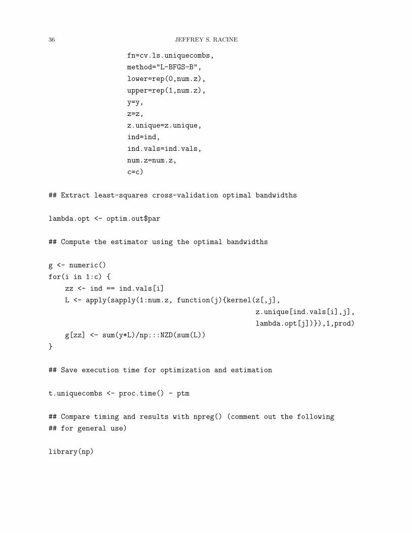
36 JEFFREY S. RACINE
fn=cv.ls.uniquecombs,
method="L-BFGS-B",
lower=rep(0,num.z),
upper=rep(1,num.z),
y=y,
z=z,
z.unique=z.unique,
ind=ind,
ind.vals=ind.vals,
num.z=num.z,
c=c)
## Extract least-squares cross-validation optimal bandwidths
lambda.opt <- optim.out$par
## Compute the estimator using the optimal bandwidths
g <- numeric()
for(i in 1:c) {
zz <- ind == ind.vals[i]
L <- apply(sapply(1:num.z, function(j){kernel(z[,j],
z.unique[ind.vals[i],j],
lambda.opt[j])}),1,prod)
g[zz] <- sum(y*L)/np:::NZD(sum(L))
}
## Save execution time for optimization and estimation
t.uniquecombs <- proc.time() - ptm
## Compare timing and results with npreg() (comment out the following
## for general use)
library(np)

PACKAGE NP FAQ 37
g.Formula <- "y ~"
for (p in 1:k) {
g.Formula <- paste(g.Formula," + factor(z[,",p,"])")
}
g.Formula <- formula(g.Formula)
t.npreg <- system.time(g.npreg <- npreg(g.Formula,
ukertype="liracine",
nmulti=1))
## Compare fitted values for first 10 observations
cbind(g[1:10],fitted(g.npreg)[1:10])
## Compare bandwidths
cbind(lambda.opt,g.npreg$bws$bw)
## Compare objective function values
cbind(optim.out$value,g.npreg$bws$fval)
## Compare computation time in seconds
cbind(t.uniquecombs[1],t.npreg[1])
2.53. I want to bootstrap the standard errors for the coefficients in a varying
coefficient specification. Is there a simple way to accomplish this? The code below
presents one way to accomplish this. For this example the model is
Yi = α(Zi) +Xiβ(Zi) + εi,
where Xi is experience and Zi is tenure. The estimated slope vector β(Zi) is therefore a
function of tenure. We bootstrap its standard error and then plot the resulting estimate and
95% asymptotic confidence bounds.
library(np)
data(wage1)
## Fit the model

38 JEFFREY S. RACINE
model <- with(wage1,npscoef(tydat=lwage,
txdat=exper,
tzdat=tenure,
betas=TRUE))
beta2 <- coef(model)[,2]
## Bootstrap the standard error for the slope coefficient (there
## will be two coefficient vectors, the intercept and slope
## for exper, which vary with tenure)
B <- 100
coef.mat <- matrix(NA,nrow(wage1),B)
for(b in 1:B) {
## Bootstrap the training data, evaluate on the original
## sample realizations, hold the bandwidth constant at
## that for the original model/training data
wage1.boot <- wage1[sample(1:nrow(wage1),replace=TRUE),]
model.boot <- with(wage1.boot,npscoef(tydat=lwage,
txdat=exper,
tzdat=tenure,
exdat=wage1$exper,
ezdat=wage1$tenure,
betas=TRUE,
bws=model$bw))
coef.mat[,b] <- coef(model.boot)[,2]
}
se.beta2 <- apply(coef.mat,1,sd)
ci.l <- beta2-1.96*se.beta2
ci.u <- beta2+1.96*se.beta2
ylim <- range(c(beta2,ci.l,ci.u))
with(wage1,plot(tenure,beta2,ylim=ylim))
with(wage1,points(tenure,ci.l,col=2))
with(wage1,points(tenure,ci.u,col=2))
legend("topleft",c("beta2","ci.l","ci.u"),col=c(1,2,2),pch=c(1,1,1),bty="n")

PACKAGE NP FAQ 39
References
[1] Francisco Cribari-Neto and Spyros G Zarkos. R: Yet another econometric programming en-
vironment. Journal of Applied Econometrics, 14(3):319–29, May-June 1999. Available at
http://ideas.repec.org/a/jae/japmet/v14y1999i3p319-29.html.
[2] Yves Croissant. Ecdat: Data sets for econometrics, 2011. R package version 0.1-6.1.
[3] Grant V. Farnsworth. Econometrics in R. Technical report, October 2008. Available at http://cran.r-
project.org/doc/contrib/Farnsworth-EconometricsInR.pdf.
[4] T. Hastie and R. Tibshirani. Generalized additive models. Chapman and Hall, London, 1990.
[5] Tristen Hayfield and Jeffrey S. Racine. Nonparametric econometrics: The np package. Journal of Sta-
tistical Software, 27(5), 2008.
[6] C. Hsiao, Q. Li, and J. Racine. A consistent model specification test with mixed categorical and con-
tinuous data. Journal of Econometrics, 140:802–826, 2007.
[7] Christian Kleiber and Achim Zeileis. Applied Econometrics with R. Springer-Verlag, New York, 2008.
ISBN 978-0-387-77316-2.
[8] Q. Li and S. Wang. A simple consistent bootstrap test for a parametric regression functional form.
Journal of Econometrics, 87:145–165, 1998.
[9] J. S. Racine. An efficient cross–validation algorithm for window width selection for nonparametric kernel
regression. Communications in Statistics, 22(4):1107–1114, October 1993.
[10] J. S. Racine. Nonparametric econometrics: A primer. Foundations and Trends in Econometrics, 3(1):1–
88, 2008.
[11] J. S. Racine and R. Hyndman. Using R to teach econometrics. Journal of Applied Econometrics,
17(2):175–189, 2002.
[12] Hao Yu. Rmpi: Interface (Wrapper) to MPI (Message-Passing Interface), 2001. R package version 0.5-8.
40 JEFFREY S. RACINE
Changes from Version 0.60-7 to 0.60-8 [04-Jun-2018]
• Used patch suggested by Scott Thompson for issue https://github.com/JeffreyRacine/R-
Package-np/issues/8 regarding npcdens()/npcdist() and formulas
Changes from Version 0.60-6 to 0.60-7 [01-May-2018]
• Fix for switch() and zero length character strings that affected summary output for
certain tests
• Added function for shape constrained bounded univariate PDF and CDF estimation
(npuniden.sc())
• Added option for renormalizing improper bounded density estimates than can
arise from the use of asymmetric negative edge kernel functions (proper=TRUE,
npuniden.boundary())
• Fixed issues with CDF estimation in the presence of large bandwidths for bounded
density estimates (npuniden.boundary())
Changes from Version 0.60-5 to 0.60-6 [12-Jan-2018]
• Added more edge kernel functions for npuniden.boundary(), some glitches addressed
• Added asymptotic standard errors and integrated density (CDF) to npuniden.boundary()
and npuniden.reflect() plus additional examples
• Added least squares cross-validation to npuniden.boundary() (default for boundary
kernel functions)
Changes from Version 0.60-4 to 0.60-5 [04-Jan-2018]
• Added two basic functions for univariate bounded kernel density estimation,
npuniden.boundary and npuniden.reflect
• More plotting routines accept more passable parameters
Changes from Version 0.60-3 to 0.60-4 [03-Dec-2017]
• Default plot.errors.style changed to "band"
• Using wrapLines(strwrap(...)) for summary output for model specification test
to automatically wrap long formula lines
• plot() calls npplot() and npplot() behaves better when most passable parameters
are fed (col =, lty =, xlab =, etc.) but there may still be room for improvement

PACKAGE NP FAQ 41
• Added option plot.par.mfrow=TRUE/FALSE to npplot() so that the automated set-
ting of par(mfrow=c(,)) in plot is disabled and the user can do this manually if
desired
• Option plot.par.mfrow=TRUE/FALSE can be overridden by setting options(plot.par.mfrow=TRUE/FALSE)
Changes from Version 0.60-2 to 0.60-3 [29-Apr-2017]
• Fixed the ‘cannot find function is()’ glitch that just surfaced with R 3.4.0
• Fixed glitch in npconmode() when randomizing if all probabilities are equal
• Migrated some code from crs (which I wrote) to avoid crs:::
• Fixed outstanding glitch in npscoef() with tydat
• Option leave.one.out not properly implemented in npscoef(), corrected
• Using pmin/pmax in NZD (parallel min/max more efficient with vectors)
• Improved screen i/o when smooth.residuals=TRUE/FALSE
• Corrected glitch in npregiv() where multivariate z would halt with error
• npregiv() with method="Landweber-Fridman" no longer passes back lists
• Fixed glitch in Kmat.lp with p=0 and derivatives
• Tikhonov regularization in npregiv() now supports evaluation data
• Updated npregiv() (was sorely lacking, did not support eval etc.)
• Use of .onLoad suggested (by Bernd Bischl)
• Added vignette("entropy_np",package="np") to startup message
• In np.distribution.bw.R default for do.full.integral changed to FALSE
• Fixed the CDF objective function when averaging over the training data
• Fixed crash error with npcdistbw() and adaptive bandwidths
Changes from Version 0.60-1 to 0.60-2 [27-Jun-2014]
• added timeseries support for all relevant objects (i.e. for a ts() vector data object x,
npreg(x~lag(x,-1)+lag(x,-2)) is now supported)
• added total time to summary for bandwidth objects
• npqreg() no longer accepts gradients=TRUE when gradients are in fact not supported
• npqreg() fails with an informative message when passed a conditional density band-
width object
Changes from Version 0.60-0 to 0.60-1 [6-Jun-2014]
• Fixed glitch in adaptive nn/generalized nn bandwidths that affected all routines that
rely on non-fixed bandwidths

42 JEFFREY S. RACINE
• Tweaks to search for adaptive nn/generalized nn initial search values
• Fixed glitch in local linear estimation with adaptive nn bandwidths
Changes from Version 0.50-1 to 0.60-0 [1-Jun-2014]
• Ordered kernel types now default to liracine/liracine (normalized) for condi-
tional/unconditional objects, respectively (the previous default, i.e. the Wang van
Ryzin kernel, is poorly behaved when smoothing out of ordered predictors is appro-
priate)
• Added analytical ordered CDF kernels, resulting in significant speedups for cross
validation with ordered variables
• Added analytical ordered convolution kernels, resulting in significant speedups for
least-squares cross validation with ordered variables
• The entire C backend has been rewritten and improved in almost every regard
• The Rmpi backend has been updated to Rmpi version 0.6-5
• Glitch in adaptive convolution kernels corrected
• Added truncated gaussian kernel (see ntpgauss() for modifying the truncation ra-
dius)
• Support for trees complete (use options(np.tree=TRUE)) which when used in con-
junction with bounded kernels (i.e. "epanechnikov"/"truncated gaussian") can
reduce the computational burden for certain problems
• Optimizers that make use of Powell’s direction set method now accept additional
arguments that can be used to potentially improve default settings
• Default search settings for optimizers that make use of Powell’s direction set method
should better scale to the range of variables
• Added mean absolute deviation/1.4826 to mix of robust scale elements
• Corrected error in order of conditional density/distribution manual bandwidths
pointed out by Decet Romain
• Figure in vignette not displaying properly, needed png=TRUE reported by Christophe
Bontemps
• Using chol2inv/chol rather than solve throughout R routines that rely on inversion
• Fixed glitch in npindexbw() to stop maxit from blowing up every time convergence
fails
• Fixed issue with summary reporting incorrect value of objective function in certain
bandwidth objects

PACKAGE NP FAQ 43
• When nmulti > 1, the full multi-starting search history is now returned in a vector
named fval.history
• Added na.action for consistency with other R functions such as lm()
• New function npquantile() that returns smooth univariate quantiles
• npksum() explicitly only uses raw bandwidths now (and will emit an error if passed
numeric scale factors, bandwidth objects are still OK)
• Fixed regression in npindex() with bootstrapped standard errors
• Code makes use of one call to npksum() in npindex() and npscoef() where possible
rather than two separate calls
• Updated npsigtest() for addition of power and added joint test to the mix
• Changed ceiling() to max(1,round()) in b.star() per Dimitris Politis’s sugges-
tion
• Reworked the interface for npcopula() to avoid two bandwidths and density=TRUE
but exploiting passing of either npudistbw() (copula) or npudensbw (copula density)
Changes from Version 0.40-13 to 0.50-1 [13-Mar-2013]
• The functions npudist() and npudistbw() are now uncoupled from npudens() and
npudensbw() (previously they relied on unconditional PDF bandwidths due to the
lack of a multivariate mixed-data method for selecting bandwidths for CDFs - now
with Li & Racine (2013) we have a robust method hence the split)
• The use of cdf=TRUE is deprecated for npudens() and npudensbw() objects due to
the uncoupling described above
• Fixed glitch in gradient standard errors in npindex() where identical standard
errors were output in model$gerr
• Fixed glitch in covariance matrix in npindex() ("ichimura") where covariance ma-
trix was not symmetric
• Fixed glitch in npksum where use of bwtype="adaptive_nn" and opera-
tor="integral" produced the survivor function rather than the cumulative distri-
bution function
• Cleaned up internals for npcmstest()
• Using .onUnload rather than .Last.lib in zzz.R
• Fixed glitch in npreg() summary where ‘Residual standard error’ was reporting
residual variance
• npksum() functionality extended

44 JEFFREY S. RACINE
– npksum() can now return the matrix of kernel weights (which can be useful for
constrained estimation, by way of illustration, or constructing novel kernel-based
procedures without the need to write extensive code)
– npksum() can now accept different operators on a product kernel, for example,
npksum(txdat=data.frame(x1,x2),operator=c("derivative","normal"),bws=c(1,1))
will use the derivative kernel for x1 (i.e. the derivative of the gaussian kernel)
and the default kernel for x2 (i.e. a standard kernel such as the gaussian) thereby
allowing the user to program a number of estimators such as conditional CDFs
etc. that were previously not available via npksum()
• Fixed glitch with variable scope where certain objects could not be found in the
environment
• Added function npcopula() for d-dimensional copula estimation via inversion
• Modified stopping rules in npregiv() and npregivderiv()
• Added reference to R2 measure (Doksum and Samarov (1995))
• Startup message points to the faq, faq is now a vignette
Changes from Version 0.40-12 to 0.40-13 [05-Mar-2012]
• Added new function npregivderiv() that implements the IV derivative method of
Florens and Racine (2012)
• Added more passable parameters to npregiv() (multistarting, parameters passed to
optim() for cross-validation)
• Changes to code to improve compliance with R ‘Writing portable packages’ guidelines
and correct partial argument matches
Changes from Version 0.40-11 to 0.40-12 [24-Nov-2011]
• Added option (user request) to hold the bandwidth fixed but optimize the parameters
in the single index model
Changes from Version 0.40-10 to 0.40-11 [24-Oct-2011]
• Corrected code regression in single index errors introduced inadvertently in 0.40-10
Changes from Version 0.40-9 to 0.40-10 [24-Oct-2011]
• Modified Silverman’s adaptive measure of spread to reflect changes in sd() (sd on
matrix deprecated)

PACKAGE NP FAQ 45
Changes from Version 0.40-8 to 0.40-9 [30-July-2011]
• Renamed COPYING file to COPYRIGHTS
Changes from Version 0.40-7 to 0.40-8 [29-July-2011]
• Fixed issue where calling npplot resets system seed
• Updated examples in docs so that plot is recommended throughout (and not npplot
that is invoked by plot)
• Fixed regression in npindex when gradients=TRUE and errors=TRUE
• Function npindex/npindexbw now accepts additional arguments and implements this
properly (i.e. proper implementation by Tristen of Version 0.30-8/0.30-9 change for
npindex)
• Function npplreg now supports factors in the parametric part just like lm() does
Changes from Version 0.40-6 to 0.40-7 [8-Jun-2011]
• Function npregiv now supports exogenous X and multivariate Z and W .
• demo(npregiv) provides a useful illustration.
Changes from Version 0.40-5 to 0.40-6 [1-Jun-2011]
• Added a new function npregiv that conducts nonparametric instrumental regression
a la Darolles, Fan, Florens and Renault (2011, Econometrica) and Horowitz (2011,
Econometrica). Note that this function currently returns the fitted ϕ(z) (i.e. lacks
much functionality relative to other np functions) and is in ‘beta status’ until further
notice.
• Added a new dataset Engel95 that allows one to estimate Engel curves using the
new nonparametric instrumental regression function npregiv.
Changes from Version 0.40-4 to 0.40-5 [26-Apr-2011]
• Fixed issue with npindexbw where, for certain problems, starting values needed re-
finement otherwise convergence would fail (we now use an improved normalization
for the starting values)
Changes from Version 0.40-3 to 0.40-4 [21-Jan-2011]
• Fixed issue with ckertype and ckerorder not being propagated in np.singleindex.bw.R
• Fixed issue with negative penalties being returned by bwmethod="cv.aic" in npregbw
(ought to have been +infinity)
46 JEFFREY S. RACINE
• Error being thrown by system(..., intern=TRUE) when mpi.quit() is called,
changed to FALSE (change to system() behaviour detailed in R CHANGELOG
2.12.0)
Changes from Version 0.40-1 to 0.40-3 [23-Jul-2010]
• Added random seed (defaults to 42) to npscoefbw to ensure consistent values for
optimization for successive invocations on the same data
• Fixed glitch in multistarting in npscoefbw whereby multistarting was not working
(always returned last computed function value and not the minimum)
• Fixed issue for npRmpi where the C code underlying regression cross-validation (code
in jksum.c) differs between np and npRmpi (both are correct with the latter being
a tad slower)
• Fixed a scope issue whereby a user would write a function that calls an np/npRmpi
command, however, objects passed to the user’s function and called by the np/npRmpi
command (i.e. such as newdata) cannot be found in the environment yet they exist
outside of the function
• Fixed issue with bwscaling=TRUE and bwmethod="cv.aic" in npreg
Changes from Version 0.40-0 to 0.40-1 [4-Jun-2010]
• Added asymptotic standard errors to npindex for the Klein and Spady and Ichimura
parameter estimates which, when gradients=TRUE, can be extracted via vcov(foo)
where foo is a npsingleindex object (the Z-scores can be obtained via Z <-
coef(foo)[-1]/sqrt(diag(vcov(foo)))[-1])
Changes from Version 0.30-9 to 0.40-0 [25-May-2010]
• Modified codebase to enable dynamic spawning for interactive sessions in npRmpi
• Interactive examples supported in npRmpi
Changes from Version 0.30-8 to 0.30-9 [17-May-2010]
• Fixed issue where ukertype and okertype were being ignored by npscoef
• Fixed code regression (dating to version 0.30-4) where random.seed=42 was not ini-
tialized in functions npcmstest, npdeneqtest, npindexbw, npsdeptest, npqcmstest,
npsigtest, npsymtest, npunitest, and npplot
• Fixed issue with saving and restoring random seed in npdeptest
• Changes to codebase to modify method used to prevent division by zero

PACKAGE NP FAQ 47
• New vignette for the npRmpi package (vignette("npRmpi",package="npRmpi"))
Changes from Version 0.30-7 to 0.30-8 [20-Apr-2010]
• Implemented moment version of metric entropy in npsymtest and npunitest with
warnings about their use documented carefully and exceptions trapped and warnings
issuing when detected
• Cleaned up print/summary output formatting of some functions
Changes from Version 0.30-6 to 0.30-7 [15-Feb-2010]
• Added function npunitest for entropy-based testing of equality of univariate densi-
ties as described in Maasoumi and Racine (2002)
• Updated vignette to reflect new functions from 0.30-4 upwards (Table 1: np functions)
Changes from Version 0.30-5 to 0.30-6 [3-Feb-2010]
• Added function npsdeptest for entropy-based testing of nonlinear serial dependence
described in Granger, Maasoumi and Racine (2004)
• Added function npdeptest for entropy-based testing of nonlinear pairwise depen-
dence described in Maasoumi and Racine (2002)
• Added more bootstrap options to npsymtest (now both iid and time-series boot-
strapping are supported)
• Cleaned up summary formatting in the vignette by adding \usepackage[utf8x]{inputenc}
to the Sweave file np.Rnw
• Fixed issue with saving and restoring random seed when there was none in the envi-
ronment
Changes from Version 0.30-4 to 0.30-5 [29-Jan-2010]
• Added function npdeneqtest for integrated squared difference testing of equality of
densities as described in Maasoumi, Li, and Racine (2009), Journal of Econometrics
• Save random seed prior to setting seed in certain functions, then restore seed after
function completes
Changes from Version 0.30-3 to 0.30-4 [27-Jan-2010]
• Added function npsymtest for entropy-based testing of symmetry described in Maa-
soumi and Racine (2009), Econometric Reviews

48 JEFFREY S. RACINE
• Added function b.star that automates block length selection for the stationary and
circular bootstrap
• Cleaned up docs
Changes from Version 0.30-2 to 0.30-3 [28-May-2009]
• Corrected error in Epanechnikov convolution kernels for fixed and generalized band-
width objects
• Changed default example in npscoef
Changes from Version 0.30-1 to 0.30-2 [19-Apr-2009]
• min(std,IQR/1.348) is the adaptive measure of spread. We now test for the patho-
logical case where IQR=0 but std>0 and return std in this instance
Changes from Version 0.30-0 to 0.30-1 [29-Jan-2009]
• predict() now supports bandwidth, density, distribution, conbandwidth, condensity,
and condistribution objects
• Consistently allow predictions for categorical values outside of support of training
data
Note that predictions based upon unconditional density objects defined over cate-
gorical variables that lie outside the support of the training data may no longer be
true probabilities (i.e., as defined over the training data and the extended/augmented
support – their sum may exceed one) and may therefore require renormalization by
the user
• Fixed a numerical issue which could hinder npregbw()’s cross validation with higher-
order kernels
• Default nmulti in npplregbw() is now set correctly
• Fixed a bug with the ridging routine in npscoefbw(), added ridging to npscoef()
• Fixed minor i/o issue with Multistart 1 of... using npscoefbw()
Changes from Version 0.20-4 to 0.30-0 [15-Jan-2009]
• Added basic user-interrupt checking for all underlying C code so that either <Ctrl-
C> (Rterm) or the ‘STOP’ icon (Rgui) will interrupt all running processes. This
has a number of desirable side effects in addition to being able to interrupt C-based
processes including i) R no longer showing up as ‘not responding’ under the task

PACKAGE NP FAQ 49
manager (Windows) or the activity monitor (Mac OS X) and ii) buffered output now
being correctly displayed when using Rgui under Windows and Mac OS X
Note that repeated interruption of large jobs can reduce available memory under
R - if this becomes an issue (i.e., you get a ‘cannot allocate...’ error under R) simply
restart R (i.e., exit then run a fresh R session)
• Added a function npseed() that allows the user to set/reset the random seed for all
underlying C routines
• Fixed a bug that caused npplregbw() to ignore any kernel options for the regression
of y on z
• Refined certain constants used in the normal-reference density bandwidth rule for
increased accuracy
• Moved from using the maximum likelihood estimate of variance throughout to the
degrees of freedom corrected estimate (all variance estimates now change by the factor
(n-1)/n)
Changes from Version 0.20-3 to 0.20-4 [19-Nov-2008]
• Using an adaptive measure of spread throughout. The scale factor reported for a
bandwidth can appear to be small when the sample standard deviation of the asso-
ciated variable is inflated due to the presence of outliers. Furthermore, supplying a
scale factor of, say, 1.06 for density estimation when there are outliers that inflate
the standard deviation may oversmooth rather dramatically in the presence of out-
liers. We now use the measure found in Silverman (1986, equation (3.30)) which
is min(standard deviation, interquartile range/1.349). This robust choice produces
expected results for scale factors in the presence of outliers
Changes from Version 0.20-2 to 0.20-3[14-Nov-2008]
• Fixed a typo which caused predict() and plot() to abort when called on plre-
gression objects, and which also prevented print() and summary() from printing
information about the kernels used when called on plregression objects
• Fixed a typo which caused partially linear regressions to crash when out-of-sample
responses were provided with evaluation data
Changes from Version 0.20-1 to 0.20-2 [02-Nov-2008]
• Allow for evaluation outside of discrete support of factors in npksum() and fixed a
warning in jksum

50 JEFFREY S. RACINE
• Fixed a bug which lead to unpredictable behavior when there were more categorical
values for the training data than realisations
Changes from Version 0.20-0 to 0.20-1 [13-Aug-2008]
• Work-around for scale-factor issues during npregbw() cv when changing the training
data
Changes from Version 0.14-3 to 0.20-0 [28-Jul-2008]
• npksum() now supports an expanded set of kernels (including convolution, derivative
and integral), which can be selected via the operator = argument
• Automatic bandwidth searches are now performed when attempting to evaluate on
data without bandwidths. This allows users to combine bandwidth selection and
estimation in one step
• The npsigtest() interface is brought in line with other functions (S3)
• Significance tests can now be performed on npreg() outputs, so npsigtest(modelname)
is now supported
• Added a vignette and faq. To see the vignette try vignette("np",package="np")
• summary() on npconmode() now properly retrieves names from bandwidth objects
• Fixed the 6th and 8th order epanechnikov kernels
• Fixed some quietness issues
• npplot() now returns data upon request for conditional densities
• npreg() and npcdens() now take the appropriate limits in some pathological cases
• User supplied bandwidths now operate seamlessly with the formula interface
Changes from Version 0.14-2 to 0.14-3 [02-May-2008]
• Fixed a glitch that only arose when using the liracine unordered kernel in the pres-
ence of irrelevant variables. The upper bound for numerical search was constrained
to be (c-1)/c [that for the aitchisonaitken unordered kernel] but ought to have
been 1. The summary output would therefore show a value of lambda hitting the
(smaller) upper bound (c-1)/1 when it may have hit the (larger) upper bound 1
Changes from Version 0.14-1 to 0.14-2 [11-Jan-2008]
• Relaxed checking tolerances slightly to prevent spurious ’invalid bandwidth’ errors
• Empty sections were removed from help files
PACKAGE NP FAQ 51
• example(foobar) now works again. This was disabled in 0.14-1 at the request of
the R maintainers in order to shorten the duration of R CMD check. All examples
remained in the help files but due to the presence of ‘dontrun’ they were not run
when example(foobar) is requested. Now a limited subset is run while the full set
of examples remain in the documents
Changes from Version 0.13-1 to 0.14-1 [18-Dec-2007]
• Now use optim() for minimisation in single index and smooth coefficient models
• Fixed bug in klein-spady objective function
• Standard errors are now available in the case of no continuous variables
• Summary should look prettier, print additional information
• Tidied up lingering issues with out-of-sample data and conditional modes
• Fixed error when plotting asymptotic errors with conditional densities
• Fixed a bug in npplot() with partially linear regressions and plot.behavior="data"
or "plot-data"
• Maximum default number of multistarts is 5
• Least-squares cross-validation of conditional densities uses a new, much faster algo-
rithm
• New, faster algorithm for least-squares cross-validation for both local-constant and
local linear regressions
Note that the estimator has changed somewhat: both cross-validation and the
estimator itself use a method of shrinking towards the local constant estimator when
singularity would otherwise lead to the breakdown of the estimator. This arises in
sparse data settings in conjunction with small bandwidths for one or more regressor
• Optimised smooth coefficient code, added ridging
• Fixed bug in uniform CDF kernel
• Fixed bug where npindexbw() would ignore bandwidth.compute = FALSE and com-
pute bandwidths when supplied with a preexisting bw object
• Now can handle estimation out of discrete support
• Summary would misreport the values of discrete scale factors which were computed
with bwscaling = TRUE
Changes from Version 0.12-1 to 0.13-1 [03-May-2007]
• Bandwidths are now checked for validity based on their variable and kernel types
• np now does a better job of preserving names of some ’y’ data
52 JEFFREY S. RACINE
• Names of coefficients returned from coef() now match variable names
• Fixed some corner cases in npksum() involving the dimensionality of outputs
• Fixed deprecation warnings in R 2.5.0 caused by use of $ on atomic objects
• Various and sundry bug fixes in npscoef()
• npscoef() now handles discrete ’z’ data
• Predict now accepts the argument ’se.fit’, like predict.lm
• Fixed bug where incorrect asymptotic standard errors of gradients for regression
objects were being displayed in npplot()
• Fixed bug where errors of gradients of regression objects were not being returned in
matrix form
• vcov() now works with partially linear regression objects
• Fixed detection of evaluation responses when using the formula interface
• Pre-computed bandwidth objects are now provided for some of the more computa-
tionally burdensome examples
• Added Jeffrey Wooldridge’s WAGE1 dataset with qualitative variables (married, fe-
male, nonwhite)
• Predictions outside of discrete support for regressions and conditional densities are
now allowed
• Fixed sign issue with scaling of standard errors in the single index model
• Fixed error when calculating some bandwidths/scale factors for display purposes
• Bug in passing certain arguments to npcdensbw() fixed
• Added predict method for qregression objects
• Proper normalisation for liracine kernel shown in summary
• Fixed output bug ( H) in summary method for sigtest objects
• Fixed regression with plotting of bootstrapped errors in perspective plots
• npcdist() no longer incorrectly calls npcdens()
• Fixed spacing between var name and p-value in significance test summaries
Version 0.12-1 [19-Nov-2006]
• Initial release of the np package on CRAN