Embed Size (px)
Citation preview

Package ‘samplingbook’May 23, 2017
Type Package
Title Survey Sampling Procedures
Version 1.2.2
Date 2017-05-21
Author Juliane Manitz <[email protected]>, contributions by MarkHempelmann <[email protected]>, Goeran Kauermann
<[email protected]>, Helmut Kuechenhoff
<[email protected]>, Shuai Shao
<[email protected]>, Cornelia Oberhauser
<[email protected]>, Nina Westerheide
<[email protected]>, Manuel Wiesenfarth
Maintainer Juliane Manitz <[email protected]>
Depends pps, sampling, survey
Description Sampling procedures from the book 'Stichproben - Methodenund praktische Umsetzung mit R' by Goeran Kauermann and HelmutKuechenhoff (2010).
License GPL (>= 2)
LazyLoad yes
NeedsCompilation no
Repository CRAN
Date/Publication 2017-05-23 03:38:31 UTC
R topics documented:samplingbook-package . . . . . . . . . . . . . . . . . . . . . . . . . . . . . . . . . . . 2election . . . . . . . . . . . . . . . . . . . . . . . . . . . . . . . . . . . . . . . . . . . 3htestimate . . . . . . . . . . . . . . . . . . . . . . . . . . . . . . . . . . . . . . . . . . 5influenza . . . . . . . . . . . . . . . . . . . . . . . . . . . . . . . . . . . . . . . . . . . 7mbes . . . . . . . . . . . . . . . . . . . . . . . . . . . . . . . . . . . . . . . . . . . . . 8
1

2 samplingbook-package
money . . . . . . . . . . . . . . . . . . . . . . . . . . . . . . . . . . . . . . . . . . . . 11pop . . . . . . . . . . . . . . . . . . . . . . . . . . . . . . . . . . . . . . . . . . . . . 12pps.sampling . . . . . . . . . . . . . . . . . . . . . . . . . . . . . . . . . . . . . . . . 13sample.size.mean . . . . . . . . . . . . . . . . . . . . . . . . . . . . . . . . . . . . . . 15sample.size.prop . . . . . . . . . . . . . . . . . . . . . . . . . . . . . . . . . . . . . . 16Smean . . . . . . . . . . . . . . . . . . . . . . . . . . . . . . . . . . . . . . . . . . . . 18Sprop . . . . . . . . . . . . . . . . . . . . . . . . . . . . . . . . . . . . . . . . . . . . 19stratamean . . . . . . . . . . . . . . . . . . . . . . . . . . . . . . . . . . . . . . . . . . 21stratasamp . . . . . . . . . . . . . . . . . . . . . . . . . . . . . . . . . . . . . . . . . . 22stratasize . . . . . . . . . . . . . . . . . . . . . . . . . . . . . . . . . . . . . . . . . . 23submean . . . . . . . . . . . . . . . . . . . . . . . . . . . . . . . . . . . . . . . . . . . 25tax . . . . . . . . . . . . . . . . . . . . . . . . . . . . . . . . . . . . . . . . . . . . . . 26wage . . . . . . . . . . . . . . . . . . . . . . . . . . . . . . . . . . . . . . . . . . . . . 27
Index 29
samplingbook-package Survey Sampling Procedures
Description
Sampling procedures from the book ’Stichproben - Methoden und praktische Umsetzung mit R’ byGoeran Kauermann and Helmut Kuechenhoff (2010).
Details
Package: SamplingbookType: PackageVersion: 1.2.1Date: 2016-07-05License: GPL(>=2)LazyLoad: yes
Index:
election German Parliament Election Datahtestimate Horvitz-Thompson Estimatorinfluenza Population and Cases of Influenza in Administrative Districts of Germanymbes Model Based Estimationmoney Money Data Framepop Small Suppositious Sampling Examplepps.sampling Sampling with Probabilities Proportional to Sizesample.size.mean Sample Size Calculation for Mean Estimationsample.size.prop Sample Size Calculation for Proportion EstimationSamplingbook-package Survey Sampling ProceduresSmean Sampling Mean Estimation

election 3
Sprop Sampling Proportion Estimationstratamean Stratified Sample Mean Estimationstratasamp Sample Size Calculation for Stratified Samplingtax Hypothetical Tax Refund Data Frame
Author(s)
Author: Juliane Manitz <[email protected]>, contributions byMark Hempelmann <[email protected]>,Goeran Kauermann <[email protected]>,Helmut Kuechenhoff <[email protected]>,Shuai Shao <[email protected]>,Cornelia Oberhauser <[email protected]>,Nina Westerheide <[email protected]>,Manuel Wiesenfarth <[email protected]>
Maintainer: Juliane Manitz <[email protected]>
References
Kauermann, Goeran/Kuechenhoff, Helmut (2010): Stichproben. Methoden und praktische Umset-zung mit R. Springer.
election German Parliament Election Data
Description
Data frame with number of citizens eligible to vote and results of the elections in 2002 and 2005for the German Bundestag, the first chamber of the German parliament.
Usage
data(election)
Format
A data frame with 299 observations (corresponding to constituencies) on the following 13 variables.
state factor, the 16 German federal states
eligible_02 number of citizens eligible to vote in 2002
SPD_02 a numeric vector, percentage for the Social Democrats SPD in 2002
UNION_02 a numeric vector, percentage for the conservative Christian Democrats CDU/CSU in2002
GREEN_02 a numeric vector, percentage for the Greens in 2002

4 election
FDP_02 a numeric vector, percentage for the Liberal Party FDP in 2002
LEFT_02 a numeric vector, percentage for the Left Party PDS in 2002
eligible_05 number of citizens eligible to vote in 2005
SPD_05 a numeric vector, percentage for the Social Democrats SPD in 2005
UNION_05 a numeric vector, percentage for the conservative Christian Democrats CDU/CSU in2005
GREEN_05 a numeric vector, percentage for the Greens in 2005
FDP_05 a numeric vector, percentage for the Liberal Party FDP in 2005
LEFT_05 a numeric vector, percentage for the Left Party in 2005
Details
German Federal Elections
Half of the Members of the German Bundestag are elected directly from Germany’s 299 constituen-cies, the other half one on the parties’ land lists. Accordingly, each voter has two votes in the elec-tions to the German Bundestag. The first vote, allowing voters to elect their local representatives tothe Bundestag, decides which candidates are sent to Parliament from the constituencies. The secondvote is cast for a party list. And it is this second vote that determines the relative strengths of theparties represented in the Bundestag. At least 598 Members of the German Bundestag are electedin this way. In addition to this, there are certain circumstances in which some candidates win whatare known as ’overhang mandates’ when the seats are being distributed.
The data set provides the percentage of second votes for each party, which determines the numberof seats each party gets in parliament. These percentages are calculated by the number of votes fora party divided by number of valid votes.
Source
The data is provided by the R package flexclust.
References
Kauermann, Goeran/Kuechenhoff, Helmut (2010): Stichproben. Methoden und praktische Umset-zung mit R. Springer.
Homepage of the Bundestag: http://www.bundestag.de.
Friedrich Leisch. A Toolbox for K-Centroids Cluster Analysis. Computational Statistics and DataAnalysis, 51 (2), 526-544, 2006.
Examples
data(election)summary(election)
# 1) Draw a simple sample of size n=20n <- 20set.seed(67396)index <- sample(1:nrow(election), size=n)sample1 <- election[index,]

htestimate 5
Smean(sample1$SPD_02, N=nrow(election))# true meanmean(election$SPD_02)
# 2) Estimate sample size to forecast proportion of SPD in election of 2005sample.size.prop(e=0.01, P=mean(election$SPD_02), N=Inf)
# 3) Usage of previous knowledge by model based estimation# draw sample of size n = 20N <- nrow(election)set.seed(67396)sample <- election[sort(sample(1:N, size=20)),]# secondary information SPD in 2002X.mean <- mean(election$SPD_02)# forecast proportion of SPD in election of 2005mbes(SPD_05 ~ SPD_02, data=sample, aux=X.mean, N=N, method='all')# true valueY.mean <- mean(election$SPD_05)Y.mean# Use a second predictor variableX.mean2 <- c(mean(election$SPD_02),mean(election$GREEN_02))# forecast proportion of SPD in election of 2005 with two predictorsmbes(SPD_05 ~ SPD_02+GREEN_02, data=sample, aux=X.mean2, N=N, method= 'regr')
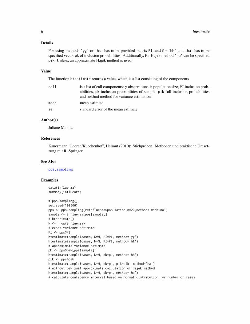
htestimate Horvitz-Thompson Estimator
Description
Calculates Horvitz-Thompson estimate with different methods for variance estimation such as Yatesand Grundy, Hansen-Hurwitz and Hajek.
Usage
htestimate(y, N, PI, pk, pik, method = 'yg')
Arguments
y vector of observationsN integer for population sizePI square matrix of second order inclusion probabilities with n rows and cols. It is
necessary to be specified for variance estimation by methods 'ht' and 'yg'.pk vector of first order inclusion probabilities of length n for the sample elements. It
is necessary to be specified for variance estimation by methods 'hh' and 'ha'.pik an optional vector of first order inclusion probabilities of length N for the popu-
lation elements . It can be used for variance estimation by method 'ha'.method method to be used for variance estimation. Options are 'yg' (Yates and Grundy)
and 'ht' (Horvitz-Thompson), approximate options are 'hh' (Hansen-Hurwitz)and 'ha' (Hajek).
6 htestimate
Details
For using methods 'yg' or 'ht' has to be provided matrix PI, and for 'hh' and 'ha' has to bespecified vector pk of inclusion probabilities. Additionally, for Hajek method 'ha' can be specifiedpik. Unless, an approximate Hajek method is used.
Value
The function htestimate returns a value, which is a list consisting of the components
call is a list of call components: y observations, N population size, PI inclusion prob-abilities, pk inclusion probabilities of sample, pik full inclusion probabilitiesand method method for variance estimation
mean mean estimate
se standard error of the mean estimate
Author(s)
Juliane Manitz
References
Kauermann, Goeran/Kuechenhoff, Helmut (2010): Stichproben. Methoden und praktische Umset-zung mit R. Springer.
See Also
pps.sampling
Examples
data(influenza)summary(influenza)
# pps.sampling()set.seed(108506)pps <- pps.sampling(z=influenza$population,n=20,method='midzuno')sample <- influenza[pps$sample,]# htestimate()N <- nrow(influenza)# exact variance estimatePI <- pps$PIhtestimate(sample$cases, N=N, PI=PI, method='yg')htestimate(sample$cases, N=N, PI=PI, method='ht')# approximate variance estimatepk <- pps$pik[pps$sample]htestimate(sample$cases, N=N, pk=pk, method='hh')pik <- pps$pikhtestimate(sample$cases, N=N, pk=pk, pik=pik, method='ha')# without pik just approximate calculation of Hajek methodhtestimate(sample$cases, N=N, pk=pk, method='ha')# calculate confidence interval based on normal distribution for number of cases

influenza 7
est.ht <- htestimate(sample$cases, N=N, PI=PI, method='ht')est.ht$mean*Nlower <- est.ht$mean*N - qnorm(0.975)*N*est.ht$seupper <- est.ht$mean*N + qnorm(0.975)*N*est.ht$sec(lower,upper)# true number of influenza casessum(influenza$cases)
influenza Population and Cases of Influenza for Administrative Districts of Ger-many
Description
The data frame influenza provides cases of influenza and inhabitants for administrative districtsof Germany in 2007.
Usage
data(influenza)
Format
A data frame with 424 observations on the following 4 variables.
id a numeric vector
district a factor with levels LK Aachen, LK Ahrweiler, ..., SK Zweibruecken, names of admin-istrative districts in Germany
population a numeric vector specifying the number of inhabitants in the specific administrativedistrict
cases a numeric vector specifying the number of influenza cases in the specific administrativedistrict
Details
Data of 2007. If you want to use the population numbers in the future, be aware of local govern-mental reorganizations, e.g. district unions.
Source
Database SurvStat of Robert Koch-Institute. Many thanks to Hermann Claus.
References
Database of Robert Koch-Institute http://www3.rki.de/SurvStat/
Kauermann, Goeran/Kuechenhoff, Helmut (2010): Stichproben. Methoden und praktische Umset-zung mit R. Springer.

8 mbes
Examples
data(influenza)summary(influenza)
# 1) Usage of pps.samplingset.seed(108506)pps <- pps.sampling(z=influenza$population,n=20,method='midzuno')ppssample <- influenza[pps$sample,]sample
# 2) Usage of htestimateset.seed(108506)pps <- pps.sampling(z=influenza$population,n=20,method='midzuno')sample <- influenza[pps$sample,]# htestimate()N <- nrow(influenza)# exact variance estimatePI <- pps$PIhtestimate(sample$cases, N=N, PI=PI, method='ht')htestimate(sample$cases, N=N, PI=PI, method='yg')# approximate variance estimatepk <- pps$pik[pps$sample]htestimate(sample$cases, N=N, pk=pk, method='hh')pik <- pps$pikhtestimate(sample$cases, N=N, pk=pk, pik=pik, method='ha')# without pik just approximative calculation of Hajek methodhtestimate(sample$cases, N=N, pk=pk, method='ha')# calculate confidence interval based on normal distribution for number of casesest.ht <- htestimate(sample$cases, N=N, PI=PI, method='ht')est.ht$mean*Nlower <- est.ht$mean*N - qnorm(0.975)*N*est.ht$seupper <- est.ht$mean*N + qnorm(0.975)*N*est.ht$sec(lower,upper)# true number of influenza casessum(influenza$cases)
mbes Model Based Estimation
Description
mbes is used for model based estimation of population means using auxiliary variables. Difference,ratio and regression estimates are available.
Usage
mbes(formula, data, aux, N = Inf, method = 'all', level = 0.95, ...)

mbes 9
Arguments
formula object of class formula (or one that can be coerced to that class): symbolicdescription for connection between primary and secondary information
data data frame containing variables in the model
aux known mean of auxiliary variable, which provides secondary information
N positive integer for population size. Default is N=Inf, which means that calcu-lations are carried out without finite population correction.
method estimation method. Options are 'simple','diff','ratio','regr','all'.Default is method='all'.
level coverage probability for confidence intervals. Default is level=0.95.
... further options for linear regression model
Details
The option method='simple' calculates the simple sample estimation without using the auxiliaryvariable. The option method='diff' calculates the difference estimate, method='ratio' the ratioestimate, and method='regr' the regression estimate which is based on the selected model. Theoption method='all' calculates the simple and all model based estimates. For methods 'diff','ratio' and 'all' the formula has to be y~x with y primary and x secondary information. Formethod 'regr', it is the symbolic description of the linear regression model. In this case, it canbe used more than one auxiliary variable. Thus, aux has to be a vector of the same length as thenumber of auxiliary variables in order as specified in the formula.
Value
The function mbes returns an object, which is a list consisting of the components
call is a list of call components: formula formula, data data frame, aux given valuefor mean of auxiliary variable, N population size, type type of model basedestimation and level coverage probability for confidence intervals
info is a list of further information components: N population size, n sample size, pnumber of auxiliary variables, aux true mean of auxiliary variables in populationand x.mean sample means of auxiliary variables
simple is a list of result components, if method='simple' or method='all' is selected:mean mean estimate of population mean for primary information, se standarderror of the mean estimate, and ci vector of confidence interval boundaries
diff is a list of result components, if method='diff' or method='all' is selected:mean mean estimate of population mean for primary information, se standarderror of the mean estimate, and ci vector of confidence interval boundaries
ratio is a list of result components, if method='ratio' or method='all' is selected:mean mean estimate of population mean for primary information, se standarderror of the mean estimate, and ci vector of confidence interval boundaries
regr is a list of result components, if type='regr' or type='all' is selected: meanmean estimate of population mean for primary information, se standard error ofmean estimate, ci vector of confidence interval boundaries, and model underly-ing linear regression model

10 mbes
Author(s)
Juliane Manitz
References
Kauermann, Goeran/Kuechenhoff, Helmut (2010): Stichproben. Methoden und praktische Umset-zung mit R. Springer.
See Also
Smean, Sprop
Examples
## 1) simple suppositious exampledata(pop)# Draw a random sample of size=3set.seed(802016)data <- pop[sample(1:5, size=3),]names(data) <- c('id','x','y')# difference estimatormbes(formula=y~x, data=data, aux=15, N=5, method='diff', level=0.95)# ratio estimatormbes(formula=y~x, data=data, aux=15, N=5, method='ratio', level=0.95)# regression estimatormbes(formula=y~x, data=data, aux=15, N=5, method='regr', level=0.95)
## 2) Bundestag electiondata(election)# draw sample of size n = 20N <- nrow(election)set.seed(67396)sample <- election[sort(sample(1:N, size=20)),]# secondary information SPD in 2002X.mean <- mean(election$SPD_02)# forecast proportion of SPD in election of 2005mbes(SPD_05 ~ SPD_02, data=sample, aux=X.mean, N=N, method='all')# true valueY.mean <- mean(election$SPD_05)Y.mean# Use a second predictor variableX.mean2 <- c(mean(election$SPD_02),mean(election$GREEN_02))# forecast proportion of SPD in election of 2005 with two predictorsmbes(SPD_05 ~ SPD_02+GREEN_02, data=sample, aux=X.mean2, N=N, method= 'regr')
## 3) money sampledata(money)mu.X <- mean(money$X)x <- money$X[which(!is.na(money$y))]y <- na.omit(money$y)# estimationmbes(y~x, aux=mu.X, N=13, method='all')

money 11
## 4) model based two-phase sampling with mbes()id <- 1:1000x <- rep(c(1,0,1,0),times=c(10,90,70,830))y <- rep(c(1,0,NA),times=c(15,85,900))phase <- rep(c(2,1), times=c(100,900))data <- data.frame(id,x,y,phase)# mean of x out of first phasemean.x <- mean(data$x)mean.xN1 <- length(data$x)# calculation of estimation for yest.y <- mbes(y~x, data=data, aux=mean.x, N=N1, method='ratio')est.y# correction of standard error with uncertaincy in first phasev.y <- var(data$y, na.rm=TRUE)se.y <- sqrt(est.y$ratio$se^2 + v.y/N1)se.y# corrected confidence intervallower <- est.y$ratio$mean - qnorm(0.975)*se.yupper <- est.y$ratio$mean + qnorm(0.975)*se.yc(lower, upper)
money Money Data Frame
Description
Data provides guesses and true values for students wallet money.
Usage
data(money)
Format
A data frame with 13 observations (corresponding to the students) on the following 3 variables.
id a numeric vector of identification number
X a numeric vector of secondary information, guesses of money in the wallet
y a numeric vector of primary information, counted money in the wallet. NA means subject was notincluded into the sample.
Details
In a lesson an experiment was made, in which the students were asked to guess the current amountof money in their wallet. A simple sample of these students was drawn, who counted the moneyin their wallet exactly. Using this secondary information, model based estimation of the populationmean is possible.

12 pop
References
Kauermann, Goeran/Kuechenhoff, Helmut (2010): Stichproben. Methoden und praktische Umset-zung mit R. Springer.
Examples
data(money)print(money)
# Usage of mbes()mu.X <- mean(money$X)x <- money$X[which(!is.na(money$y))]y <- na.omit(money$y)# estimationmbes(y~x, aux=mu.X, N=13, method='all')
pop Small Suppositious Sampling Example
Description
pop is a suppositious data frame for a small population with 5 elements. It is used for simpleillustration of survey sampling estimators.
Usage
data(pop)
Format
A data frame with 5 observations on the following 3 variables.
id a numeric vector of individual identification values
X a numeric vector of first characteristic
Y a numeric vector of second characteristic
References
Kauermann, Goeran/Kuechenhoff, Helmut (2010): Stichproben. Methoden und praktische Umset-zung mit R. Springer.

pps.sampling 13
Examples
data(pop)print(pop)
## 1) Usage of Smean()data(pop)Y <- pop$YY# Draw a random sample pop size=3set.seed(93456)y <- sample(x = Y, size = 3)sort(y)# Estimation with infiniteness correctionest <- Smean(y = y, N = length(pop$Y))est
## 2) Usage of mbes()data(pop)# Draw a random sample of size=3set.seed(802016)data <- pop[sample(1:5, size=3),]names(data) <- c('id','x','y')# difference estimatormbes(formula=y~x, data=data, aux=15, N=5, method='diff', level=0.95)# ratio estimatormbes(formula=y~x, data=data, aux=15, N=5, method='ratio', level=0.95)# regression estimatormbes(formula=y~x, data=data, aux=15, N=5, method='regr', level=0.95)
pps.sampling Sampling with Probabilities Proportional to Size
Description
The function provides sample techniques with sampling probabilities which are proportional to thesize of a quantity z.
Usage
pps.sampling(z, n, id = 1:N, method = 'sampford', return.PI = FALSE)
Arguments
z vector of quantities which determine the sampling probabilities in the population
n positive integer for sample size
id an optional vector with identification values for population elements. Default is'id = 1:N', where 'N' is length of 'z'.

14 pps.sampling
method the sampling method to be used. Options are 'sampford', 'tille', 'midzuno'or 'madow'.
return.PI logical. If TRUE the pairwise inclusion probabilities for all individuals in thepopulation are returned.
Details
The different methods vary in their run time. Therefore, method='sampford' is stopped if N > 200or if n/N < 0.3. method='tille' is stopped if N > 500. In case of large populations usemethod='midzuno' or method='madow'.
Value
The function pps.sampling returns a value, which is a list consisting of the components
call is a list of call components: z vector of quantity data, n sample size, id identifi-cation values, and method sampling method
sample resulted sample
pik inclusion probabilities
PI sample second order inclusion probabilities
PI.full full second order inclusion probabilities
Author(s)
Juliane Manitz
References
Kauermann, Goeran/Kuechenhoff, Helmut (2010): Stichproben. Methoden und praktische Umset-zung mit R. Springer.
See Also
htestimate
Examples
## 1) simple suppositious exampledata <- data.frame(id = 1:7, z = c(1.8, 2 ,3.2 ,2.9 ,1.5 ,2.0 ,2.2))# Usage of pps.sampling for Sampford methodset.seed(178209)pps.sample_sampford <- pps.sampling(z=data$z, n=2, method='sampford', return.PI=FALSE)pps.sample_sampford# sampling elementsid.sample <- pps.sample_sampford$sampleid.sample# other methodsset.seed(178209)pps.sample_tille <- pps.sampling(z=data$z, n=2, method='tille')pps.sample_tille
sample.size.mean 15
set.seed(178209)pps.sample_midzuno <- pps.sampling(z=data$z, n=2, method='midzuno')pps.sample_midzunoset.seed(178209)pps.sample_madow <- pps.sampling(z=data$z, n=2, method='madow')pps.sample_madow
## 2) influenzadata(influenza)summary(influenza)
set.seed(108506)pps <- pps.sampling(z=influenza$population,n=20,method='midzuno')ppssample <- influenza[pps$sample,]sample
sample.size.mean Sample Size Calculation for Mean Estimation
Description
The function sample.size.mean returns the sample size needed for mean estimations either withor without consideration of finite population correction.
Usage
sample.size.mean(e, S, N = Inf, level = 0.95)
Arguments
e positive number specifying the precision which is half width of confidence in-terval
S standard deviation in population
N positive integer for population size. Default is N=Inf, which means that calcu-lations are carried out without finite population correction.
level coverage probability for confidence intervals. Default is level=0.95.
Value
The function sample.size.mean returns a value, which is a list consisting of the components
call is a list of call components: e precision, S standard deviation in population, andN integer for population size
n estimate of sample size
Author(s)
Juliane Manitz

16 sample.size.prop
References
Kauermann, Goeran/Kuechenhoff, Helmut (2010): Stichproben. Methoden und praktische Umset-zung mit R. Springer.
See Also
Smean, sample.size.prop
Examples
# sample size for precision e=4sample.size.mean(e=4,S=10,N=300)# sample size for precision e=1sample.size.mean(e=1,S=10,N=300)
sample.size.prop Sample Size Calculation for Proportion Estimation
Description
The function sample.size.prop returns the sample size needed for proportion estimation eitherwith or without consideration of finite population correction.
Usage
sample.size.prop(e, P = 0.5, N = Inf, level = 0.95)
Arguments
e positive number specifying the precision which is half width of confidence in-terval
P expected proportion of events with domain between values 0 and 1. Default isP=0.5.
N positive integer for population size. Default is N=Inf, which means that calcu-lations are carried out without finite population correction.
level coverage probability for confidence intervals. Default is level=0.95.
Details
For meaningful calculation, precision e should be chosen smaller than 0.5, because the domainof P is between values 0 and 1. Furthermore, precision e should be smaller than proportion P,respectively (1-P).

sample.size.prop 17
Value
The function sample.size.prop returns a value, which is a list consisting of the components
call is a list of call components e precision, P expected proportion, N population size,and level coverage probability for confidence intervals
n estimate of sample size
Author(s)
Juliane Manitz
References
Kauermann, Goeran/Kuechenhoff, Helmut (2010): Stichproben. Methoden und praktische Umset-zung mit R. Springer.
See Also
Sprop, sample.size.mean
Examples
## 1) examples with different precisions# precision 1% for election forecast of SPD in 2005sample.size.prop(e=0.01, P=0.5, N=Inf)data(election)sample.size.prop(e=0.01, P=mean(election$SPD_02), N=Inf)# precision 5% for questionnairesample.size.prop(e=0.05, P=0.5, N=300)sample.size.prop(e=0.05, P=0.5, N=Inf)# precision 10%sample.size.prop(e=0.1, P=0.5, N=300)sample.size.prop(e=0.1, P=0.5, N=1000)
## 2) tables in the book# table 2.2P_vector <- c(0.2, 0.3, 0.4, 0.5)N_vector <- c(10, 100, 1000, 10000)results <- matrix(NA, ncol=4, nrow=4)for (i in 1:length(P_vector)){
for (j in 1:length(N_vector)){x <- try(sample.size.prop(e=0.1, P=P_vector[i], N=N_vector[j]))if (class(x)=='try-error') {results[i,j] <- NA}else {results[i,j] <- x$n}
}}dimnames(results) <- list(paste('P=',P_vector, sep=''), paste('N=',N_vector, sep=''))results# table 2.3P_vector <- c(0.5, 0.1)e_vector <- c(0.1, 0.05, 0.03, 0.02, 0.01)

18 Smean
results <- matrix(NA, ncol=2, nrow=5)for (i in 1:length(e_vector)){
for (j in 1:length(P_vector)){x <- try(sample.size.prop(e=e_vector[i], P=P_vector[j], N=Inf))if (class(x)=='try-error') {results[i,j] <- NA}else {results[i,j] <- x$n}
}}dimnames(results) <- list(paste('e=',e_vector, sep=''), paste('P=',P_vector, sep=''))results
Smean Sampling Mean Estimation
Description
The function Smean estimates the population mean out of simple samples either with or withoutconsideration of finite population correction.
Usage
Smean(y, N = Inf, level = 0.95)
Arguments
y vector of sample data
N positive integer specifying population size. Default is N=Inf, which means thatcalculations are carried out without finite population correction.
level coverage probability for confidence intervals. Default is level=0.95.
Value
The function Smean returns a value, which is a list consisting of the components
call is a list of call components: y vector with sample data, n sample size, N popula-tion size, level coverage probability for confidence intervals
mean mean estimate
se standard error of the mean estimate
ci vector of confidence interval boundaries
Author(s)
Juliane Manitz

Sprop 19
References
Kauermann, Goeran/Kuechenhoff, Helmut (2010): Stichproben. Methoden und praktische Umset-zung mit R. Springer.
See Also
Sprop, sample.size.mean
Examples
data(pop)Y <- pop$YY# Draw a random sample of size=3set.seed(93456)y <- sample(x = Y, size = 3)sort(y)# Estimation with infiniteness correctionest <- Smean(y = y, N = length(pop$Y))est
Sprop Sampling Proportion Estimation
Description
The function Sprop estimates the proportion out of samples either with or without considerationof finite population correction. Different methods for calculating confidence intervals for examplebased on binomial distribution (Agresti and Coull or Clopper-Pearson) or based on hypergeometricdistribution are used.
Usage
Sprop(y, m, n = length(y), N = Inf, level = 0.95)
Arguments
y vector of sample data containing values 0 and 1m an optional non-negative integer for number of positive eventsn an optional positive integer for sample size. Default is n=length(y).N positive integer for population size. Default is N=Inf, which means calculations
are carried out without finite population correction.level coverage probability for confidence intervals. Default is level=0.95.
Details
Sprop can be called by usage of a data vector y with the observations 1 for event and 0 for failure.Moreover, it can be called by specifying the number of events m and trials n.

20 Sprop
Value
The function Sprop returns a value, which is a list consisting of the components
call is a list of call components: y sample data, m number of positive events in thesample, n sample size, N population size, level coverage probability for confi-dence intervals
p proportion estimate
se standard error of the proportion estimate
ci is a list of confidence interval boundaries for proportion.In case of a finite population of size N, it is given approx, the hypergeometricconfidence interval with normal distribution approximation, and exact, the ex-act hypergeometric confidence interval.If the population is very large N=Inf, it is calculated bin, the binomial confi-dence interval, which is asymptotic, cp the exact confidence interval based onbinomial distribution (Clopper-Pearson), and ac, the asymptotic confidence in-terval based on binomial distribution by Wilson (Agresti and Coull (1998)).
nr In case of finite population of size N, it is given a list of confidence intervalboundaries for number in population with approx, the hypergeometric confi-dence interval with normal distribution approximation, and exact, the exacthypergeometric confidence interval.
Author(s)
Juliane Manitz
References
Kauermann, Goeran/Kuechenhoff, Helmut (2010): Stichproben. Methoden und praktische Umset-zung mit R. Springer.
Agresti, Alan/Coull, Brent A. (1998): Approximate Is Better than ’Exact’ for Interval Estimationof Binomial Proportions. The American Statistician, Vol. 52, No. 2 , pp. 119-126.
See Also
Smean, sample.size.prop
Examples
# 1) Survey in company to upgrade office climateSprop(m=45, n=100, N=300)Sprop(m=2, n=100, N=300)
# 2) German opinion poll for 03/07/09 with# (http://www.wahlrecht.de/umfragen/politbarometer.htm)# a) 302 of 1206 respondents who would elect SPD.# b) 133 of 1206 respondents who would elect the Greens.Sprop(m=302, n=1206, N=Inf)Sprop(m=133, n=1206, N=Inf)

stratamean 21
# 3) Rare disease of animals (sample size n=500 of N=10.000 animals, one infection)# for 95% one sided confidence level use level=0.9Sprop(m=1, n=500, N=10000, level=0.9)
# 4) call with data vector yy <- c(0,0,1,0,1,0,0,0,1,1,0,0,1)Sprop(y=y, N=200)# is the same asSprop(m=5, n=13, N=200)
stratamean Stratified Sample Mean Estimation
Description
The function stratamean estimates the population mean out of stratified samples either with orwithout consideration of finite population correction.
Usage
stratamean(y, h, Nh, wh, level = 0.95, eae = FALSE)
Arguments
y vector of target variable.
h vector of stratifying variable.
Nh vector of sizes of every stratum, which has to be supplied in alphabetical ornumerical order of the categories of h.
wh vector of weights of every stratum, which has to be supplied in alphabetical ornumerical order of the categories of h.
level coverage probability for confidence intervals. Default is level=0.95.
eae TRUE for extensive output with the result in each and every stratum. Default iseae=FALSE.
Details
If the absolute stratum sizes Nh are given, the variances are calculated with finite population cor-rection. Otherwise, if the stratum weights wh are given, the variances are calculated without finitepopulation correction.
Value
The function stratamean returns a value, which is a list consisting of the components
call is a list of call components: y target variable in sample data, h stratifying variablein sample data, Nh sizes of every stratum, wh weights of every stratum, fpc finitepopulation correction, level coverage probability for confidence intervals

22 stratasamp
mean mean estimate for population
se standard error of the mean estimate for population
ci vector of confidence interval boundaries for population
Author(s)
Shuai Shao and Juliane Manitz
References
Kauermann, Goeran/Kuechenhoff, Helmut (2010): Stichproben. Methoden und praktische Umset-zung mit R. Springer.
See Also
Smean, Sprop
Examples
# random datatesty <- rnorm(100)testh <- c(rep("male",40), rep("female",60))stratamean(testy, testh, wh=c(0.5, 0.5))stratamean(testy, testh, wh=c(0.5, 0.5), eae=TRUE)
# tax datadata(tax)summary(tax)
nh <- as.vector(table(tax$Class))wh <- nh/sum(nh)stratamean(y=tax$diff, h=as.vector(tax$Class), wh=wh, eae=TRUE)
stratasamp Sample Size Calculation for Stratified Sampling
Description
The function stratasamp calculates the sample size for each stratum depending on type of alloca-tion.
Usage
stratasamp(n, Nh, Sh = NULL, Ch = NULL, type = 'prop')

stratasize 23
Arguments
n positive integer specifying sampling size.
Nh vector of population sizes of each stratum.
Sh vector of standard deviation in each stratum.
Ch vector of cost for a sample in each stratum.
type type of allocation. Default is type='prop' for proportional, alternatives aretype='opt' for optimal and type='costopt' for cost-optimal.
Value
The function stratasamp returns a matrix, which lists the strata and the sizes of observation de-pending on type of allocation.
Author(s)
Shuai Shao and Juliane Manitz
References
Kauermann, Goeran/Kuechenhoff, Helmut (2010): Stichproben. Methoden und praktische Umset-zung mit R. Springer.
See Also
stratamean, stratasize, sample.size.mean
Examples
#random proportional stratified samplestratasamp(n=500, Nh=c(5234,2586,649,157))stratasamp(n=500, Nh=c(5234,2586,649,157), Sh=c(251,1165,8035,24725), type='opt')
stratasize Sample Size Determination for Stratified Sampling
Description
The function stratasize determinates the total size of stratified samples depending on type ofallocation and determinated by specified precision.
Usage
stratasize(e, Nh, Sh, level = 0.95, type = 'prop')

24 stratasize
Arguments
e positive number specifying sampling precision.
Nh vector of population sizes in each stratum.
Sh vector of standard deviation in each stratum.
level coverage probability for confidence intervals. Default is level=0.95.
type type of allocation. Default is type='prop' for proportional, alternative is type='opt'for optimal.
Value
The function stratasize returns a value, which is a list consisting of the components
call is a list of call components: e specified precision, Nh population sizes of ev-ery stratum, Sh standard diviation of every stratum, method type of allocation,level coverage probability for confidence intervals.
n determinated total sample size.
Author(s)
Shuai Shao
References
Kauermann, Goeran/Kuechenhoff, Helmut (2011): Stichproben. Methoden und praktische Umset-zung mit R. Springer.
See Also
stratasamp, stratamean
Examples
#random proportional stratified samplestratasize(e=0.1, Nh=c(100000,300000,600000), Sh=c(1,2,3))
#random optimal stratified samplestratasize(e=0.1, Nh=c(100000,300000,600000), Sh=c(1,2,3), type="opt")

submean 25
submean Sub-sample Mean Estimation
Description
The function submean estimates the population mean out of sub-samples (two-stage samples) eitherwith or without consideration of finite population correction in both stages.
Usage
submean(y, PSU, N, M, Nl, m.weight, n.weight, method = 'simple', level = 0.95)
Arguments
y vector of target variable.
PSU vector of grouping variable which indicates the primary unit for each sampleelement.
N positive integer specifying population size
M positive integer specifying the number of primary units in the population.
Nl vector of sample sizes in each primary unit, which has to be specified in alpha-betical or numerical order of the categories of l.
m.weight vector of primary sample unit weights, which has to be specified in alphabeticalor numerical order of the categories of l.
n.weight vector of secondary sample unit weights in each primary sample unit, which hasto be specified in alphabetical or numerical order of the categories of l.
method estimation method. Default is "simple", alternative is "ratio".
level coverage probability for confidence intervals. Default is level=0.95.
Details
If the absolute sizes M and Nl are given, the variances are calculated with finite population correction.Otherwise, if the weights m.weight and n.weight are given, the variances are calculated withoutfinite population correction.
Value
The function submean returns a value, which is a list consisting of the components
call is a list of call components: y target variable in sample data, PSU gouping vari-able in sample data, N population size, M number of primary population units,fpc finite population correction, method estimation method, level coverageprobability for confidence intervals
mean mean estimate for population
se standard error of the mean estimate for population
ci vector of confidence interval boundaries for population

26 tax
Author(s)
Shuai Shao and Juliane Manitz
References
Kauermann, Goeran/Kuechenhoff, Helmut (2011): Stichproben. Methoden und praktische Umset-zung mit R. Springer.
See Also
Smean, stratamean
Examples
y <- c(23,33,24,25,72,74,71,37,42)psu <- as.factor(c(1,1,1,1,2,2,2,3,3))# with finite population correctionsubmean(y, PSU=psu, N=700, M=23, Nl=c(100,50,75), method='ratio')# without finite population correctionsubmean(y, PSU=psu, N=700, m.weight=3/23, n.weight=c(4/100,3/50,2/75), method='ratio')
# Chinese wage datadata(wage)summary(wage)submean(wage$Wage,PSU=wage$Region, N=990, M=33, Nl=rep(30,14))
tax Hypothetical Tax Refund Data Frame
Description
Simulated tax refund data frame including the estimated and actual refund value
Usage
data(tax)
Format
A data frame with 9083 observations on the following 5 variables.
id a numeric vector indicating the tax payer
estRefund a numeric vector representing the estimated value of tax refund by the tax payer
actRefund a numeric vector representing the actual tax refund calculated by the financial authority
diff difference between estimated and acture tax refund
Class a factor with levels 1, 2, 3, and 4 indicating the strata

wage 27
Source
Due to data protection this is a simulated data set reflecting the real data.
References
Kauermann, Goeran/Kuechenhoff, Helmut (2010): Stichproben. Methoden und praktische Umset-zung mit R. Springer.
Examples
data(tax)summary(tax)
# illustration of stratameannh <- as.vector(table(tax$Class))wh <- nh/sum(nh)stratamean(y=tax$diff, h=as.vector(tax$Class), wh=wh, eae=TRUE)
wage Chinese wage data
Description
A data frame with hypothetical Chinese wages differenciated by region and industrial sector.
Usage
data(wage)
Format
A data frame with 231 observations on the following 3 variables.
Region factor, Chinese regions with 14 levels.
Sector factor, industrial sector with 30 levels.
Wage a numeric vector, average wage in the region and sector measured in Chinese yuan.
Details
The dataset is hypothetical. Its structure imitates the data in the Chinese Statistical Yearbook.The values are simulated corresponding to the distribution of the real data which are not publiclyaccessible.
References
Kauermann, Goeran/Kuechenhoff, Helmut (2010): Stichproben. Methoden und praktische Umset-zung mit R. Springer.

28 wage
Examples
# Chinese wage datadata(wage)summary(wage)submean(wage$Wage,PSU=wage$Region, N=990, M=33, Nl=rep(30,14))

Index
∗Topic datasetselection, 3influenza, 7money, 11pop, 12tax, 26wage, 27
election, 3
htestimate, 5, 14
influenza, 7
mbes, 8money, 11
pop, 12pps.sampling, 6, 13
sample.size.mean, 15, 17, 19, 23sample.size.prop, 16, 16, 20samplingbook (samplingbook-package), 2samplingbook-package, 2Smean, 10, 16, 18, 20, 22, 26Sprop, 10, 17, 19, 19, 22stratamean, 21, 23, 24, 26stratasamp, 22, 24stratasize, 23, 23submean, 25
tax, 26
wage, 27
29