Package ‘spatial’ - R · Package ‘spatial ’ August 30, 2015 ... object A ﬁtted trend surface model object from surf.ls... Further objects of the same kind Value

Package ‘spatial’August 30, 2015

Priority recommended

Version 7.3-11

Date 2015-08-29

Depends R (>= 3.0.0), graphics, stats, utils

Suggests MASS

Description Functions for kriging and point pattern analysis.

Title Functions for Kriging and Point Pattern Analysis

LazyLoad yes

ByteCompile yes

License GPL-2 | GPL-3

URL http://www.stats.ox.ac.uk/pub/MASS4/

NeedsCompilation yes

Author Brian Ripley [aut, cre, cph],Roger Bivand [ctb],William Venables [cph]

Maintainer Brian Ripley <[email protected]>

Repository CRAN

Date/Publication 2015-08-30 08:59:41

R topics documented:anova.trls . . . . . . . . . . . . . . . . . . . . . . . . . . . . . . . . . . . . . . . . . . 2correlogram . . . . . . . . . . . . . . . . . . . . . . . . . . . . . . . . . . . . . . . . . 3expcov . . . . . . . . . . . . . . . . . . . . . . . . . . . . . . . . . . . . . . . . . . . . 4Kaver . . . . . . . . . . . . . . . . . . . . . . . . . . . . . . . . . . . . . . . . . . . . 5Kenvl . . . . . . . . . . . . . . . . . . . . . . . . . . . . . . . . . . . . . . . . . . . . 6Kfn . . . . . . . . . . . . . . . . . . . . . . . . . . . . . . . . . . . . . . . . . . . . . 7ppgetregion . . . . . . . . . . . . . . . . . . . . . . . . . . . . . . . . . . . . . . . . . 8ppinit . . . . . . . . . . . . . . . . . . . . . . . . . . . . . . . . . . . . . . . . . . . . 8pplik . . . . . . . . . . . . . . . . . . . . . . . . . . . . . . . . . . . . . . . . . . . . . 9

1

http://www.stats.ox.ac.uk/pub/MASS4/

2 anova.trls

ppregion . . . . . . . . . . . . . . . . . . . . . . . . . . . . . . . . . . . . . . . . . . . 10predict.trls . . . . . . . . . . . . . . . . . . . . . . . . . . . . . . . . . . . . . . . . . . 11prmat . . . . . . . . . . . . . . . . . . . . . . . . . . . . . . . . . . . . . . . . . . . . 12Psim . . . . . . . . . . . . . . . . . . . . . . . . . . . . . . . . . . . . . . . . . . . . . 13semat . . . . . . . . . . . . . . . . . . . . . . . . . . . . . . . . . . . . . . . . . . . . 14SSI . . . . . . . . . . . . . . . . . . . . . . . . . . . . . . . . . . . . . . . . . . . . . . 15Strauss . . . . . . . . . . . . . . . . . . . . . . . . . . . . . . . . . . . . . . . . . . . . 16surf.gls . . . . . . . . . . . . . . . . . . . . . . . . . . . . . . . . . . . . . . . . . . . 17surf.ls . . . . . . . . . . . . . . . . . . . . . . . . . . . . . . . . . . . . . . . . . . . . 18trls.influence . . . . . . . . . . . . . . . . . . . . . . . . . . . . . . . . . . . . . . . . . 19trmat . . . . . . . . . . . . . . . . . . . . . . . . . . . . . . . . . . . . . . . . . . . . . 20variogram . . . . . . . . . . . . . . . . . . . . . . . . . . . . . . . . . . . . . . . . . . 21

Index 23

anova.trls Anova tables for fitted trend surface objects

Description

Compute analysis of variance tables for one or more fitted trend surface model objects; whereanova.trls is called with multiple objects, it passes on the arguments to anovalist.trls.

Usage

## S3 method for class 'trls'anova(object, ...)anovalist.trls(object, ...)

Arguments

object A fitted trend surface model object from surf.ls

... Further objects of the same kind

Value

anova.trls and anovalist.trls return objects corresponding to their printed tabular output.

References

Venables, W. N. and Ripley, B. D. (2002) Modern Applied Statistics with S. Fourth edition. Springer.

See Also

surf.ls

correlogram 3

Examples

library(stats)data(topo, package="MASS")topo0 <- surf.ls(0, topo)topo1 <- surf.ls(1, topo)topo2 <- surf.ls(2, topo)topo3 <- surf.ls(3, topo)topo4 <- surf.ls(4, topo)anova(topo0, topo1, topo2, topo3, topo4)summary(topo4)

correlogram Compute Spatial Correlograms

Description

Compute spatial correlograms of spatial data or residuals.

Usage

correlogram(krig, nint, plotit = TRUE, ...)

Arguments

krig trend-surface or kriging object with columns x, y, and z

nint number of bins used

plotit logical for plotting

... parameters for the plot

Details

Divides range of data into nint bins, and computes the covariance for pairs with separation in eachbin, then divides by the variance. Returns results for bins with 6 or more pairs.

Value

x and y coordinates of the correlogram, and cnt, the number of pairs averaged per bin.

Side Effects

Plots the correlogram if plotit = TRUE.

References

Ripley, B. D. (1981) Spatial Statistics. Wiley.


4 expcov

See Also

variogram

Examples

data(topo, package="MASS")topo.kr <- surf.ls(2, topo)correlogram(topo.kr, 25)d <- seq(0, 7, 0.1)lines(d, expcov(d, 0.7))

expcov Spatial Covariance Functions

Description

Spatial covariance functions for use with surf.gls.

Usage

expcov(r, d, alpha = 0, se = 1)gaucov(r, d, alpha = 0, se = 1)sphercov(r, d, alpha = 0, se = 1, D = 2)

Arguments

r vector of distances at which to evaluate the covariance

d range parameter

alpha proportion of nugget effect

se standard deviation at distance zero

D dimension of spheres.

Value

vector of covariance values.

References



See Also

surf.gls

Kaver 5

Examples

data(topo, package="MASS")topo.kr <- surf.ls(2, topo)correlogram(topo.kr, 25)d <- seq(0, 7, 0.1)lines(d, expcov(d, 0.7))

Kaver Average K-functions from Simulations

Description

Forms the average of a series of (usually simulated) K-functions.

Usage

Kaver(fs, nsim, ...)

Arguments

fs full scale for K-fn

nsim number of simulations

... arguments to simulate one point process object

Value

list with components x and y of the average K-fn on L-scale.

References



See Also

Kfn, Kenvl

Examples

towns <- ppinit("towns.dat")par(pty="s")plot(Kfn(towns, 40), type="b")plot(Kfn(towns, 10), type="b", xlab="distance", ylab="L(t)")for(i in 1:10) lines(Kfn(Psim(69), 10))lims <- Kenvl(10,100,Psim(69))lines(lims$x,lims$lower, lty=2, col="green")lines(lims$x,lims$upper, lty=2, col="green")lines(Kaver(10,25,Strauss(69,0.5,3.5)), col="red")

6 Kenvl

Kenvl Compute Envelope and Average of Simulations of K-fns

Description

Computes envelope (upper and lower limits) and average of simulations of K-fns

Usage

Kenvl(fs, nsim, ...)

Arguments

fs full scale for K-fn

nsim number of simulations

... arguments to produce one simulation

Value

list with components

x distances

lower min of K-fns

upper max of K-fns

aver average of K-fns

References



See Also

Kfn, Kaver

Examples

towns <- ppinit("towns.dat")par(pty="s")plot(Kfn(towns, 40), type="b")plot(Kfn(towns, 10), type="b", xlab="distance", ylab="L(t)")for(i in 1:10) lines(Kfn(Psim(69), 10))lims <- Kenvl(10,100,Psim(69))lines(lims$x,lims$lower, lty=2, col="green")lines(lims$x,lims$upper, lty=2, col="green")lines(Kaver(10,25,Strauss(69,0.5,3.5)), col="red")

Kfn 7

Kfn Compute K-fn of a Point Pattern

Description

Actually computes L =√K/π.

Usage

Kfn(pp, fs, k=100)

Arguments

pp a list such as a pp object, including components x and y

fs full scale of the plot

k number of regularly spaced distances in (0, fs)

Details

relies on the domain D having been set by ppinit or ppregion.

Value

A list with components

x vector of distances

y vector of L-fn values

k number of distances returned – may be less than k if fs is too large

dmin minimum distance between pair of points

lm maximum deviation from L(t) = t

References



See Also

ppinit, ppregion, Kaver, Kenvl

Examples

towns <- ppinit("towns.dat")par(pty="s")plot(Kfn(towns, 10), type="s", xlab="distance", ylab="L(t)")

8 ppinit

ppgetregion Get Domain for Spatial Point Pattern Analyses

Description

Retrieves the rectangular domain (xl, xu) × (yl, yu) from the underlying C code.

Usage

ppgetregion()

Value

A vector of length four with names c("xl", "xu", "yl", "yu").

References


See Also

ppregion

ppinit Read a Point Process Object from a File

Description

Read a file in standard format and create a point process object.

Usage

ppinit(file)

Arguments

file string giving file name

Details

The file should contain

the number of pointsa header (ignored)xl xu yl yu scalex y (repeated n times)

pplik 9

Value

class "pp" object with components x, y, xl, xu, yl, yu

Side Effects

Calls ppregion to set the domain.

References


See Also

ppregion

Examples

towns <- ppinit("towns.dat")par(pty="s")plot(Kfn(towns, 10), type="b", xlab="distance", ylab="L(t)")

pplik Pseudo-likelihood Estimation of a Strauss Spatial Point Process

Description

Pseudo-likelihood estimation of a Strauss spatial point process.

Usage

pplik(pp, R, ng=50, trace=FALSE)

Arguments

pp a pp object

R the fixed parameter R

ng use a ng x ng grid with border R in the domain for numerical integration.

trace logical? Should function evaluations be printed?

Value

estimate for c in the interval [0, 1].

References

Ripley, B. D. (1988) Statistical Inference for Spatial Processes. Cambridge.


10 ppregion

See Also

Strauss

Examples

pines <- ppinit("pines.dat")pplik(pines, 0.7)

ppregion Set Domain for Spatial Point Pattern Analyses

Description

Sets the rectangular domain (xl, xu) × (yl, yu).

Usage

ppregion(xl = 0, xu = 1, yl = 0, yu = 1)

Arguments

xl Either xl or a list containing components xl, xu, yl, yu (such as a point-processobject)

xu

yl

yu

Value

none

Side Effects

initializes variables in the C subroutines.

References


See Also

ppinit, ppgetregion

predict.trls 11

predict.trls Predict method for trend surface fits

Description

Predicted values based on trend surface model object

Usage

## S3 method for class 'trls'predict(object, x, y, ...)

Arguments

object Fitted trend surface model object returned by surf.ls

x Vector of prediction location eastings (x coordinates)

y Vector of prediction location northings (y coordinates)

... further arguments passed to or from other methods.

Value

predict.trls produces a vector of predictions corresponding to the prediction locations. To dis-play the output with image or contour, use trmat or convert the returned vector to matrix form.

References


See Also

surf.ls, trmat

Examples

data(topo, package="MASS")topo2 <- surf.ls(2, topo)topo4 <- surf.ls(4, topo)x <- c(1.78, 2.21)y <- c(6.15, 6.15)z2 <- predict(topo2, x, y)z4 <- predict(topo4, x, y)cat("2nd order predictions:", z2, "\n4th order predictions:", z4, "\n")

12 prmat

prmat Evaluate Kriging Surface over a Grid

Description

Evaluate Kriging surface over a grid.

Usage

prmat(obj, xl, xu, yl, yu, n)

Arguments

obj object returned by surf.gls

xl limits of the rectangle for grid

xu

yl

yu

n use n x n grid within the rectangle

Value

list with components x, y and z suitable for contour and image.

References



See Also

surf.gls, trmat, semat

Examples

data(topo, package="MASS")topo.kr <- surf.gls(2, expcov, topo, d=0.7)prsurf <- prmat(topo.kr, 0, 6.5, 0, 6.5, 50)contour(prsurf, levels=seq(700, 925, 25))

Psim 13

Psim Simulate Binomial Spatial Point Process

Description

Simulate Binomial spatial point process.

Usage

Psim(n)

Arguments

n number of points

Details

relies on the region being set by ppinit or ppregion.

Value

list of vectors of x and y coordinates.

Side Effects

uses the random number generator.

References



See Also

SSI, Strauss

Examples

towns <- ppinit("towns.dat")par(pty="s")plot(Kfn(towns, 10), type="s", xlab="distance", ylab="L(t)")for(i in 1:10) lines(Kfn(Psim(69), 10))

14 semat

semat Evaluate Kriging Standard Error of Prediction over a Grid

Description

Evaluate Kriging standard error of prediction over a grid.

Usage

semat(obj, xl, xu, yl, yu, n, se)

Arguments

obj object returned by surf.gls


xu

yl

yu


se standard error at distance zero as a multiple of the supplied covariance. Other-wise estimated, and it assumed that a correlation function was supplied.

Value


References



See Also

surf.gls, trmat, prmat

Examples

data(topo, package="MASS")topo.kr <- surf.gls(2, expcov, topo, d=0.7)prsurf <- prmat(topo.kr, 0, 6.5, 0, 6.5, 50)contour(prsurf, levels=seq(700, 925, 25))sesurf <- semat(topo.kr, 0, 6.5, 0, 6.5, 30)contour(sesurf, levels=c(22,25))

SSI 15

SSI Simulates Sequential Spatial Inhibition Point Process

Description

Simulates SSI (sequential spatial inhibition) point process.

Usage

SSI(n, r)

Arguments

n number of points

r inhibition distance

Details

uses the region set by ppinit or ppregion.

Value

list of vectors of x and y coordinates

Side Effects

uses the random number generator.

Warnings

will never return if r is too large and it cannot place n points.

References



See Also

Psim, Strauss

Examples

towns <- ppinit("towns.dat")par(pty = "s")plot(Kfn(towns, 10), type = "b", xlab = "distance", ylab = "L(t)")lines(Kaver(10, 25, SSI(69, 1.2)))

16 Strauss

Strauss Simulates Strauss Spatial Point Process

Description

Simulates Strauss spatial point process.

Usage

Strauss(n, c=0, r)

Arguments

n number of points

c parameter c in [0, 1]. c = 0 corresponds to complete inhibition at distances upto r.

r inhibition distance

Details

Uses spatial birth-and-death process for 4n steps, or for 40n steps starting from a binomial patternon the first call from an other function. Uses the region set by ppinit or ppregion.

Value

list of vectors of x and y coordinates

Side Effects

uses the random number generator

References



See Also

Psim, SSI

Examples

towns <- ppinit("towns.dat")par(pty="s")plot(Kfn(towns, 10), type="b", xlab="distance", ylab="L(t)")lines(Kaver(10, 25, Strauss(69,0.5,3.5)))

surf.gls 17

surf.gls Fits a Trend Surface by Generalized Least-squares

Description

Fits a trend surface by generalized least-squares.

Usage

surf.gls(np, covmod, x, y, z, nx = 1000, ...)

Arguments

np degree of polynomial surface

covmod function to evaluate covariance or correlation function

x x coordinates or a data frame with columns x, y, z

y y coordinates

z z coordinates. Will supersede x$z

nx Number of bins for table of the covariance. Increasing adds accuracy, and in-creases size of the object.

... parameters for covmod

Value


beta the coefficients

x

y

z and others for internal use only.

References



See Also

trmat, surf.ls, prmat, semat, expcov, gaucov, sphercov

18 surf.ls

Examples

library(MASS) # for eqscplotdata(topo, package="MASS")topo.kr <- surf.gls(2, expcov, topo, d=0.7)trsurf <- trmat(topo.kr, 0, 6.5, 0, 6.5, 50)eqscplot(trsurf, type = "n")contour(trsurf, add = TRUE)

prsurf <- prmat(topo.kr, 0, 6.5, 0, 6.5, 50)contour(prsurf, levels=seq(700, 925, 25))sesurf <- semat(topo.kr, 0, 6.5, 0, 6.5, 30)eqscplot(sesurf, type = "n")contour(sesurf, levels = c(22, 25), add = TRUE)

surf.ls Fits a Trend Surface by Least-squares

Description

Fits a trend surface by least-squares.

Usage

surf.ls(np, x, y, z)

Arguments

np degree of polynomial surface

x x coordinates or a data frame with columns x, y, z

y y coordinates

z z coordinates. Will supersede x$z

Value


beta the coefficients

x

y

z and others for internal use only.

References



trls.influence 19

See Also

trmat, surf.gls

Examples

library(MASS) # for eqscplotdata(topo, package="MASS")topo.kr <- surf.ls(2, topo)trsurf <- trmat(topo.kr, 0, 6.5, 0, 6.5, 50)eqscplot(trsurf, type = "n")contour(trsurf, add = TRUE)points(topo)

eqscplot(trsurf, type = "n")contour(trsurf, add = TRUE)plot(topo.kr, add = TRUE)title(xlab= "Circle radius proportional to Cook's influence statistic")

trls.influence Regression diagnostics for trend surfaces

Description

This function provides the basic quantities which are used in forming a variety of diagnostics forchecking the quality of regression fits for trend surfaces calculated by surf.ls.

Usage

trls.influence(object)## S3 method for class 'trls'plot(x, border = "red", col = NA, pch = 4, cex = 0.6,

add = FALSE, div = 8, ...)

Arguments

object, x Fitted trend surface model from surf.ls

div scaling factor for influence circle radii in plot.trls

add add influence plot to existing graphics if TRUEborder, col, pch, cex, ...

additional graphical parameters

Value

trls.influence returns a list with components:

r raw residuals as given by residuals.trls

hii diagonal elements of the Hat matrixstresid standardised residualsDi Cook’s statistic

20 trmat

References

Unwin, D. J., Wrigley, N. (1987) Towards a general-theory of control point distribution effects intrend surface models. Computers and Geosciences, 13, 351–355.


See Also

surf.ls, influence.measures, plot.lm

Examples

library(MASS) # for eqscplotdata(topo, package = "MASS")topo2 <- surf.ls(2, topo)infl.topo2 <- trls.influence(topo2)(cand <- as.data.frame(infl.topo2)[abs(infl.topo2$stresid) > 1.5, ])cand.xy <- topo[as.integer(rownames(cand)), c("x", "y")]trsurf <- trmat(topo2, 0, 6.5, 0, 6.5, 50)eqscplot(trsurf, type = "n")contour(trsurf, add = TRUE, col = "grey")plot(topo2, add = TRUE, div = 3)points(cand.xy, pch = 16, col = "orange")text(cand.xy, labels = rownames(cand.xy), pos = 4, offset = 0.5)

trmat Evaluate Trend Surface over a Grid

Description

Evaluate trend surface over a grid.

Usage

trmat(obj, xl, xu, yl, yu, n)

Arguments

obj object returned by surf.ls or surf.gls


xu

yl

yu


Value


variogram 21

References



See Also

surf.ls, surf.gls

Examples

data(topo, package="MASS")topo.kr <- surf.ls(2, topo)trsurf <- trmat(topo.kr, 0, 6.5, 0, 6.5, 50)

variogram Compute Spatial Variogram

Description

Compute spatial (semi-)variogram of spatial data or residuals.

Usage

variogram(krig, nint, plotit = TRUE, ...)

Arguments

krig trend-surface or kriging object with columns x, y, and z

nint number of bins used

plotit logical for plotting

... parameters for the plot

Details

Divides range of data into nint bins, and computes the average squared difference for pairs withseparation in each bin. Returns results for bins with 6 or more pairs.

Value

x and y coordinates of the variogram and cnt, the number of pairs averaged per bin.

Side Effects

Plots the variogram if plotit = TRUE

22 variogram

References



See Also

correlogram

Examples

data(topo, package="MASS")topo.kr <- surf.ls(2, topo)variogram(topo.kr, 25)

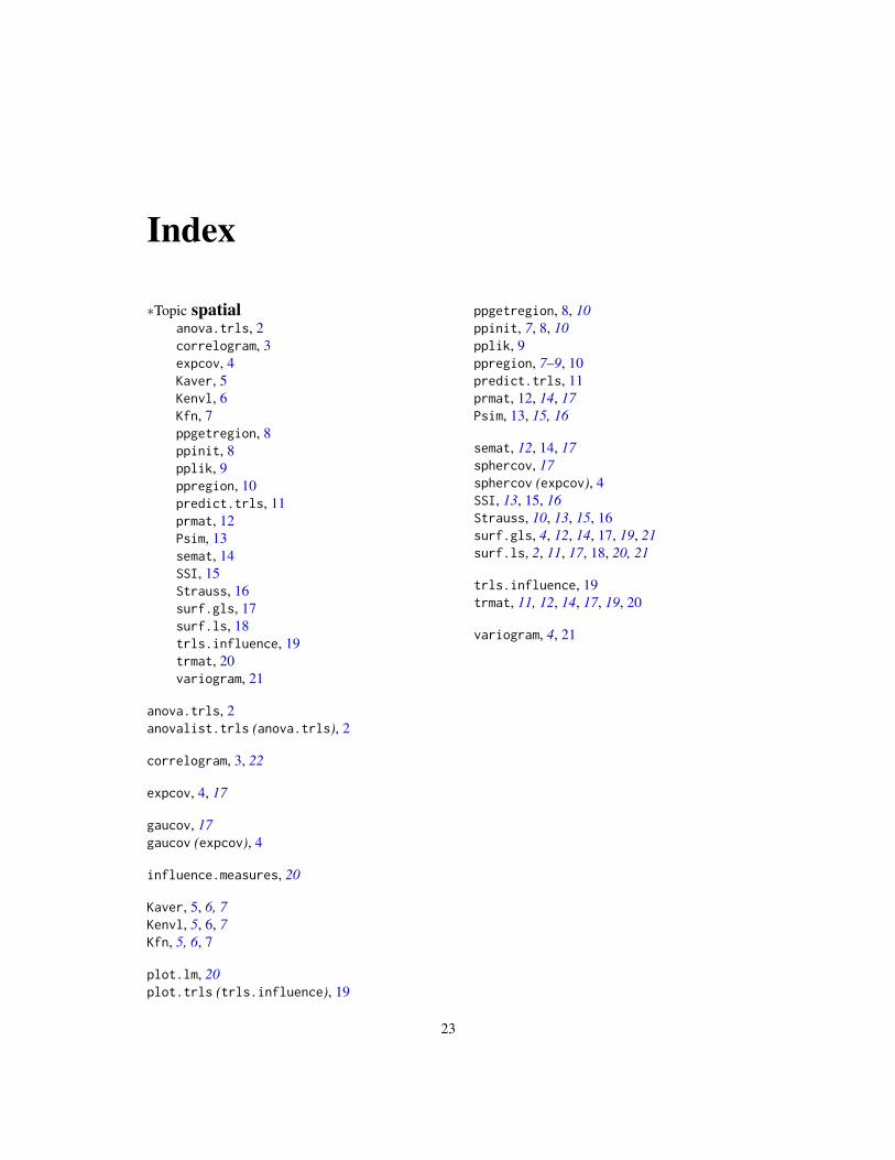
Index

∗Topic spatialanova.trls, 2correlogram, 3expcov, 4Kaver, 5Kenvl, 6Kfn, 7ppgetregion, 8ppinit, 8pplik, 9ppregion, 10predict.trls, 11prmat, 12Psim, 13semat, 14SSI, 15Strauss, 16surf.gls, 17surf.ls, 18trls.influence, 19trmat, 20variogram, 21

anova.trls, 2anovalist.trls (anova.trls), 2

correlogram, 3, 22

expcov, 4, 17

gaucov, 17gaucov (expcov), 4

influence.measures, 20

Kaver, 5, 6, 7Kenvl, 5, 6, 7Kfn, 5, 6, 7

plot.lm, 20plot.trls (trls.influence), 19

ppgetregion, 8, 10ppinit, 7, 8, 10pplik, 9ppregion, 7–9, 10predict.trls, 11prmat, 12, 14, 17Psim, 13, 15, 16

semat, 12, 14, 17sphercov, 17sphercov (expcov), 4SSI, 13, 15, 16Strauss, 10, 13, 15, 16surf.gls, 4, 12, 14, 17, 19, 21surf.ls, 2, 11, 17, 18, 20, 21

trls.influence, 19trmat, 11, 12, 14, 17, 19, 20

variogram, 4, 21

23

Documents

Package ‘spatial’ - R · Package ‘spatial ’ August 30, 2015 ... object A ﬁtted trend surface model object from surf.ls... Further objects of the same kind Value