Sequential measurement of a superconducting qubit

T. Peronnin,1 D. Markovic,2 Q. Ficheux,1 and B. Huard1

1Universite Lyon, ENS de Lyon, Universite Claude Bernard Lyon 1,CNRS, Laboratoire de Physique, F-69342 Lyon, France

2Unite Mixte de Physique, CNRS, Thales, Univ. Paris-Sud,Universite Paris-Saclay, 91767 Palaiseau, France

(Dated: April 10, 2019)

We present a superconducting device that realizes the sequential measurement of a transmonqubit. The unitary evolution between system and probe is indeed separated in time and space fromthe measurement of the probe itself. The device disables common limitations of dispersive readoutsuch as Purcell effect or transients in the cavity mode by tuning the coupling to the measurementchannel on demand. The probe is initially stored in a memory mode and coupled to the qubit untila microwave pump releases it into an output line in a characteristic time as low as 10 ns, whichis 400 times shorter than the memory lifetime. The Wigner function of the memory allows us tocharacterize the non-Gaussian nature of the probe and its dynamics. A direct measurement of thereleased probe field quadratures demonstrates a readout fidelity of 97.5 % in a total measurementtime of 220 ns.

PACS numbers:

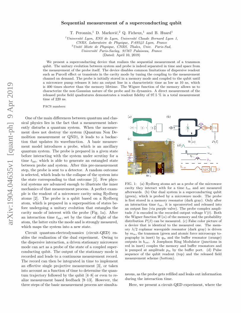
One of the main differences between quantum and clas-sical physics lies in the fact that a measurement inher-ently disturbs a quantum system. When the measure-ment does not destroy the system (Quantum Non De-molition measurement or QND), it leads to a backac-tion that updates its wavefunction. A basic measure-ment model introduces a probe, which is an ancillaryquantum system. The probe is prepared in a given statebefore interacting with the system under scrutiny for atime tint, which is able to generate an entangled statebetween probe and system. After this pre-measurementstep, the probe is sent to a detector. A random outcomeis selected, which leads to the collapse of the system intothe state corresponding to that outcome [1]. Few phys-ical systems are advanced enough to illustrate the innermechanics of that measurement process. A perfect exam-ple is the readout of a microwave cavity using Rydbergatoms [2]. The probe is a qubit based on a Rydbergatom, which is prepared in a superposition of states be-fore undergoing a unitary evolution that entangles thecavity mode of interest with the probe (Fig. 1a). Afteran interaction time tint, set by the time of flight of theatom, the latter exits the mode and is strongly measured,which maps the system into a new state.

Circuit quantum-electrodynamics (circuit-QED) en-ables the realization of the dual experiment. Owing tothe dispersive interaction, a driven stationary microwavemode can act as a probe of the state of a coupled super-conducting qubit. The output of the stationary mode isrecorded and leads to a continuous measurement record.The record can then be integrated in time to implementan effective single projective measurement [3], or takeninto account as a function of time to determine the quan-tum trajectory followed by the qubit [4–8] or even to re-alize measurement based feedback [9–13]. However, thethree steps of the basic measurement process are simulta-

FIG. 1: (a) Rydberg atoms act as a probe of the microwavecavity they interact with for a time tint and are measuredafterwards. (b) Our dual system is a superconducting qubit(green), which is probed by a microwave mode. The probeis first stored in a memory resonator (dark gray). Only afteran interaction time tint, it is upconverted and released intoan output line (via purple valve). The probe complex ampli-tude β is encoded in the recorded output voltage V (t). Boththe Wigner function W (α) of the memory and the probabilitydistribution P (β) can be measured. (c) False color picture ofa device that is identical to the measured one. The mem-ory λ/2 coplanar waveguide resonator (dark gray) is drivenby min, the transmon (green and atomic force microscopy to-pography in inset) by qin and the buffer resonator (orange)outputs in bout. A Josephson Ring Modulator (junctions inred in inset) couples the memory and buffer resonators andis pumped at amplitude pin by the buffer port. (d) Pulsesequence of the qubit readout (top) and the released fieldmeasurement scheme (bottom).

neous, as the probe gets refilled and leaks out informationduring the interaction time.

Here, we present a circuit-QED experiment, where the

arX

iv:1

904.

0463

5v1

[qu

ant-

ph]

9 A

pr 2

019

2

measurement of a qubit in the |g〉, |e〉 basis is separatedin the three sequential steps of the basic measurementmodel. It is analogous to the proposed catch-disperse-release protocol [14]. For that purpose, we have designedand realized a transmon qubit coupled to a high-Q mi-crowave resonator (memory) whose state can be flushedon-demand into an output line. The release character-istic time can be as short as 10 ns (see Fig. 1b), thusconsiderably improving a former 3D version of this de-vice [15]. The probe resonator is initialized in a coher-ent state and evolves unitarily in interaction with thequbit for a time tint. Finally the mode is released intothe transmission line and measured, thus revealing infor-mation about the qubit state. Interestingly, the schemealleviates the usual trade-off between QND measurementspeed and fidelity by disabling the link between dispersiveinteraction strength and qubit relaxation rate [16–18] andavoiding transients in resonator population [17, 19, 20],without resorting to the complexity of longitudinal cou-pling [21–23]. We obtain performances that are close tostate-of-the-art for qubit readout [18] with a fidelity of97.5 % in a total time of 220 ns.

The key element of our sequential measurement is amemory mode that couples to a qubit system and whichis able to store a microwave field and release it on-demandinto an output line. In order to realize it, we have usedan upgraded version of the Superconducting QuantumNode [15] coupled to a transmon qubit. Instead of using3D architecture as in our previous work, the device (seeFig. 1c) is made in coplanar waveguide geometry withNiobium on Silicon and Al/AlOx/Al Josephson junc-tions. The Quantum Node is made of two λ/2 resonatorsarranged as a cross and that are coupled via a JosephsonRing Modulator (JRM) in their center (inset of Fig. 1c)and is cooled down below 30 mK. The memory has a fre-quency ωm = 2π× 3.73 GHz and a lifetime Tm = 4.0 µs.The buffer resonator has a frequency ωb = 2π×10.22 GHzand is intentionally much more lossy as it is connected toan output transmission line with a rate κb = 2π×21 MHz.

Close to flux quantum in the Josephson ring, the cou-pling Hamiltonian is dominated by a three-wave mixinginteraction term between the memory mode (m), the

buffer mode (b) and a common mode of the device thatis localized in both arms [24]. When the latter is off-resonantly driven by a pump of amplitude pin and fre-quency ωp = ωb − ωm, the effective coupling is described

by the beam-splitter Hamiltonian Hbs = ~(gb†m +

g∗bm†), where the conversion rate g is proportional tothe pump amplitude pin [25]. With the addition of a fre-quency conversion between memory and buffer, turningon the pump thus results in an effective tunable couplingrate of the memory mode to the output line [15, 26, 27].In practice, we used a smoothed time dependence of the

pump amplitude pin(t) ∝(

cosh (√π/2t/σ)

)−1

in order

to turn on or off the coupling (Fig. 1d). While the mem-

ory can be emptied in a timescale as short as σmin = 10 ns[27], we obtained the highest readout fidelity for a timeσ = 28 ns, and we consider this case only in the rest ofthe letter.

The system to readout is a transmon qubit with fre-quency ωq = 2π × 4.45 GHz, lifetime T1 = 6.1 µs andcoherence time T2 = 9.2 µs. Crucially, the symmetry ofthe device is chosen to cancel out its coupling to the com-mon mode while preserving the coupling to the λ/2 modeof the memory. Therefore the large pump powers haveno detrimental effect on the transmon during release. Aprevious design without this symmetry showed that thepump would otherwise ionize the transmon [28]. Thequbit and memory are dispersively coupled so that theeffective first order interaction term reads −~χm†m|e〉〈e|where χ = 2π × 2.1 MHz. Once the qubit is prepared ina given state (Fig. 1d), the experiment starts by a dis-placement of the initially empty memory mode (via portmin) in 10 ns, which is short enough compared to 1/χto prepare the probe in the coherent state |α0〉 irrespec-tive of the qubit state. The probe is thus initialized in adeterministic state and can now interact with the qubitunder a unitary evolution for a time tint. After this time,the probe is released into the transmission line and si-multaneously upconverted to the buffer frequency usinga pump pulse. It is finally amplified and measured toextract its complex amplitude β as defined below.

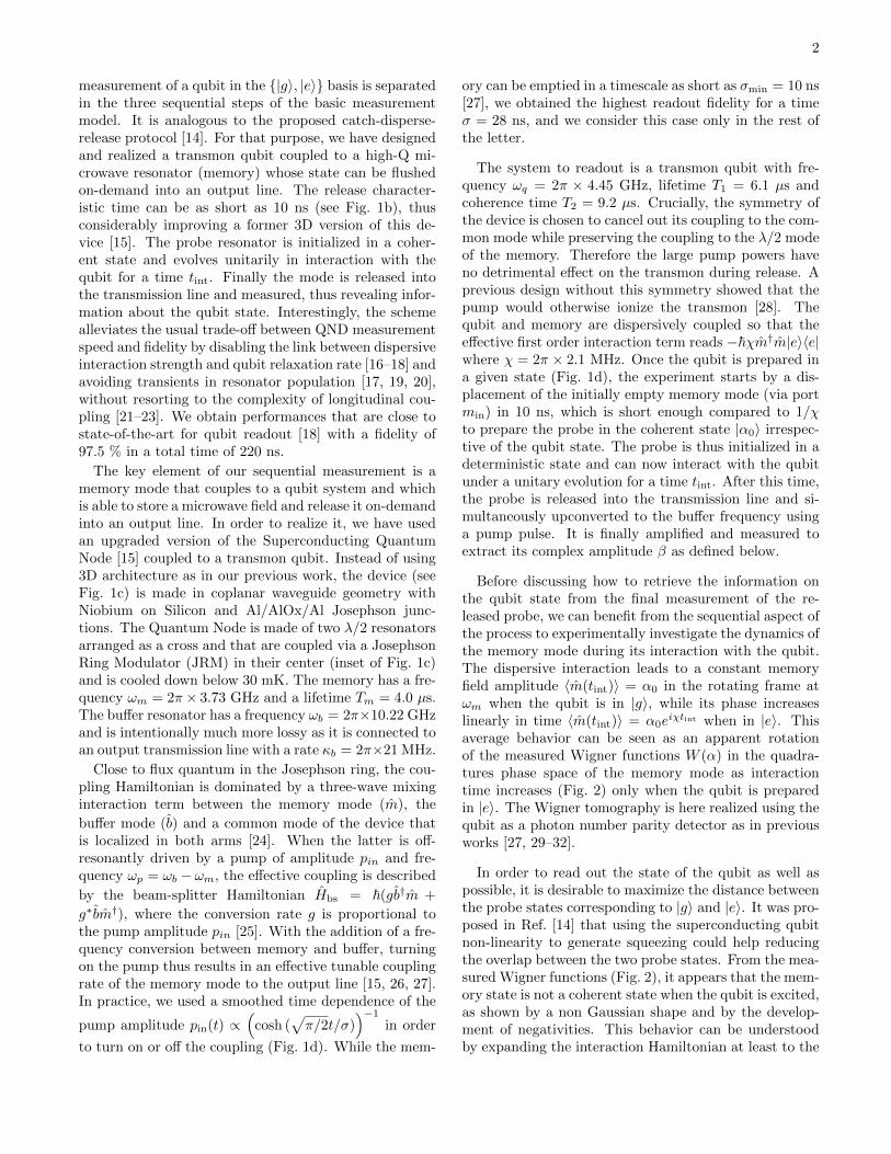
Before discussing how to retrieve the information onthe qubit state from the final measurement of the re-leased probe, we can benefit from the sequential aspect ofthe process to experimentally investigate the dynamics ofthe memory mode during its interaction with the qubit.The dispersive interaction leads to a constant memoryfield amplitude 〈m(tint)〉 = α0 in the rotating frame atωm when the qubit is in |g〉, while its phase increaseslinearly in time 〈m(tint)〉 = α0e

iχtint when in |e〉. Thisaverage behavior can be seen as an apparent rotationof the measured Wigner functions W (α) in the quadra-tures phase space of the memory mode as interactiontime increases (Fig. 2) only when the qubit is preparedin |e〉. The Wigner tomography is here realized using thequbit as a photon number parity detector as in previousworks [27, 29–32].

In order to read out the state of the qubit as well aspossible, it is desirable to maximize the distance betweenthe probe states corresponding to |g〉 and |e〉. It was pro-posed in Ref. [14] that using the superconducting qubitnon-linearity to generate squeezing could help reducingthe overlap between the two probe states. From the mea-sured Wigner functions (Fig. 2), it appears that the mem-ory state is not a coherent state when the qubit is excited,as shown by a non Gaussian shape and by the develop-ment of negativities. This behavior can be understoodby expanding the interaction Hamiltonian at least to the

3

0

800

1400

-0.20.00.20.40.60.81.0

in m

emor

yRe

leas

edQubit prepared in Qubit prepared in

0

0

8-8

8

-8

0

0

8-8

8

-80

0

8-8

8

-8

0

0

8-8

8

-8

FIG. 2: Top row: measured Wigner function W (α) of the memory state after various interaction times tint for a qubit initializedin |e〉 or |g〉 and initial coherent state amplitude α0 = 5.8 in the memory. A global rotation of the quadrature phase space wasdone numerically [27]. Bottom row: corresponding histograms of the measured complex amplitude β of the probe (see textfor definition) after it has been released into the transmission line following the interaction time tint for 105 realizations of theexperiment.

next order [33], which gives

Hint/~ = −χm†m|e〉〈e|−Kgm†2m2|g〉〈g|−Kem

†2m2|e〉〈e|.(1)

The Kerr rates could be independently measured to beKg = 2π × 8 kHz and Ke = 2π × 37 kHz [27]. Inter-estingly, the memory self-Kerr rate is much larger whenthe qubit is excited than when it is in the ground state,which explains why the Wigner function shape is littledistorted for |g〉 and strongly distorted for |e〉. A simpleway to qualitatively understand the shape of the Wignerfunction is to realize that the Kerr term induces an angu-lar velocity in the quadrature phase space that increaseswith field amplitude. A quantitative study reveals thatyet higher order terms need to be taken into account atthe large number of photons |α0|2 ≈ 34 that we are us-ing [27]. It is interesting to note that it would be possibleto use a single junction for the memory release [26]. How-ever, the JRM we use allows us to tune the cross-Kerrterms by the magnetic flux in the ring [27]. In this work,we set the flux to cancel out the cross-Kerr effects be-tween the buffer and the memory mode and between thememory mode and the common mode. Hence the strongpump does not shift the resonance frequencies.

By releasing the memory state into the output line byupconversion to ωb, we can access the information aboutthe qubit that is encoded in the memory. The emittedpulse is amplified by a Traveling Wave Parametric Am-plifier [34] followed by cryogenic and room temperatureamplifiers [27]. It is finally down-converted to 50 MHzand digitized as a voltage V (t) (Fig. 1b). A typical traceV (t) of a single realization is shown in Fig. 3a for a qubitprepared in |g〉 or |e〉. How to recover the informationabout the qubit state from the final measurement of thereleased probe field? Our solution consists in defining a

50

0.0

-50

25

0.0

-25

10

0.0

-10

1000.0 200 300

FIG. 3: (a) Raw traces of the output voltage V (t) for tworealizations of the experiment with the qubit prepared eitherin |g〉 or in |e〉 and with an initial displacement α0 = 5.8 andinteraction time tint = 100 ns. (b) Average traces over 105

realizations. (c) Real and imaginary part of the weight func-tion w(t) from which the complex amplitude of the releasedprobe is obtained.

complex amplitude β for the released probe by demod-ulating the single measurement records V (t) by a singlecomplex weight function w(t) to be determined.

β =

∫V (t)w(t)dt. (2)

We first average the traces of 105 realizations of the ex-periment for tint = 100 ns and α0 = 5.8 (Fig. 3b). Theaverages V |e,g〉(t) reveal the 50 MHz modulation we used

4

FIG. 4: (a) Scalar product of the measured distributionsPg,e(β) of released probe amplitudes when the qubit is pre-pared in |g〉 or |e〉 as a function of interaction time tint, andfor various values of initial displacement α0. (b) Same scalarproduct as a function of α0 and tint. Colored dashed linesindicate cuts corresponding to Fig. (a).

and the temporal envelope of the releasing pump pin(t).We find (see [27] for details) that a way to faithfully mapthe intraresonator complex field amplitude α to the de-modulated amplitude β, independently of the qubit state,consists in choosing a weight function w(t) whose realpart is Re[w(t)] =

(V |e〉(t)− V |g〉(t)

)/2λ (Fig. 3 c). Its

imaginary part Im[w(t)] is then constructed by shiftingthe phase of the carrier modulation by π/2. The prefac-tor λ−1 is adjusted so that β is dimensionless and equalon average to α0 in the case tint = 0. As can be seen inFig. 2, with this choice, the probability densities Pg,e(β)to measure a complex amplitude β for a qubit preparedin |g〉 and in |e〉 are indeed smoothed versions of the in-traresonator Wigner functions.

The readout operation then comes down to determin-ing whether a measured amplitude β is more likely tooccur if the qubit is in the ground or excited state. It isstraightforward once we know the distributions of com-plex amplitudes Pg(β) and Pe(β). We stress that sincethe probes are not in a Gaussian state, there is infor-mation in both quadratures, which justifies the use of aphase preserving amplifier. The 2D scalar product be-tween the histograms

〈Pg, Pe〉 =

∫C

dαPg(α)Pe(α)(∫C

dαPg(α)2)1/2 (∫

CdαPe(α)2

)1/2 (3)

quantifies the distinguishability of the measurement out-comes. Fig. 4 represents the measured overlap of the twodistributions as a function of interaction time tint and forthree values of the initial amplitude α0 of the probe inthe memory.

As mentioned above, the dispersive interaction leadsto a global rotation in the quadrature phase space of thememory mode when the qubit is in |e〉. With disper-

sive interaction alone, the even and odd integer values oftintχ/π would thus correspond to maxima and minimaof 〈Pg, Pe〉, which are reached for full turns or half turnsof the average complex amplitude of the probe. Fig. 4illustrates which phenomena determine the amplitude α0

that maximizes the readout fidelity. If α0 is too low, theseparation between the distribution supports does notovercome the noise. It is what sets the minimum overlapof the green curve at α0 = 2.1, on top of the residual in-ternal losses of the memory that dampen the oscillations.If α0 is too large, the higher order terms in the interactionHamiltonian lead to a uniform distribution in phase, andthe time oscillations disappear (red curve at α0 = 8.5).The full dependence of the overlap 〈Pg, Pe〉 as a func-tion of α0 and tint (Fig. 4b) can be used to determinethe optimal readout conditions. The minimal overlap〈Pg, Pe〉 = 3.4 % is reached at α0 = 5.8 and tint = 100 nsas in Fig. 2 and 3. Interestingly, at large amplitudes(7 < α0 < 10) the oscillations become more complicatedas a double periodicity appears and is not understood yet(red curve). At very large values (α0 > 10) the qubit isionized [28]. We note that this platform seems suited tostudy the dynamics of ionization of the qubit.

In order to characterize the measurement readout forapplications, we associate values of β where Pg(β) >Pe(β) to the measurement outcome ”g” and ”e” oth-erwise. We can then define the measurement errors Ee(respect. Eg) as obtaining the result ”g” (respect. ”e”)after having prepared the qubit in |e〉 (respect. |g〉). Wefind Ee = 3.4% and Eg = 1.6%. They can be partiallyexplained by the qubit thermal population of 0.8%, thefinite qubit lifetime and the gate fidelity 99.5%. The av-erage fidelity is F = 1 − Eg+Ee

2 = 97.5 % for a totalreadout time is 220 ns. Finally, one may wonder how therelease process affects the qubit. We have characterizedhow QND the readout is by determining the probabilityFQND = 95 % that two successive measurements find thesame outcome.

In conclusion, we have implemented the sequentialmeasurement of a transmon where the probe initializa-tion, interaction with the qubit and detection are all sep-arated in time and space. Our readout scheme is insen-sitive to the Purcell effect since it is always coupled to ahigh Q resonator except during release when the bufferresonator acts as a Purcell filter anyway. By releasingthe probe on demand, we also avoid common limitationsdue to slow reset of the cavity mode in dispersive mea-surements. The use of a JRM as a switch between thememory mode and the transmission line opens interestingperspectives. Indeed, the JRM can also act as a built-inamplifier [35, 36] (by applying a pump at the frequencyωp = ωb +ωm) to amplify the probe as it is released intothe transmission line. Besides, by increasing the partici-pation ratio of the JRM in the memory mode, one couldnot only adjust but even cancel out the Kerr rates Kg

or Ke of the memory mode by tuning the magnetic flux

5

in the JRM. Finally it would be interesting to retrievethe information that remains in the autocorrelation ofthe measured voltage V (t). Indeed, the qubit state de-pendent Kerr terms in Kg and Ke should allow for extrainformation to be retrieved in this way [37].

We thank Zaki Leghtas, Raphael Lescanne, Maz-yar Mirrahimi, Pierre Rouchon, Alain Sarlette, HubertSouquet-Basiege, Matthias Droth, and Marco Marcianifor fruitful interactions over the course of this project.The device was fabricated in the cleanrooms of Collegede France, ENS Paris, CEA Saclay, and Observatoire deParis. The Traveling Wave Amplifier was provided bythe team of Will Oliver at Lincoln labs. The project waspartly supported by Agence Nationale de la Rechercheunder project ANR-14-CE26-0018 and by the EuropeanUnions Horizon 2020 research and innovation programmeunder grant agreement No 820505.

[1] Zurek, Reviews of Modern Physics 75, 715 (2003).[2] S. Haroche, Reviews of Modern Physics 85, 1083 (2013).[3] A. Blais, J. Gambetta, A. Wallraff, D. I. Schuster, S. M.

Girvin, M. H. Devoret, and R. J. Schoelkopf, PhysicalReview A 75, 32329 (2007).

[4] J. Gambetta, A. Blais, M. Boissonneault, A. A. Houck,D. I. Schuster, and S. M. Girvin, Physical Review A 77,012112 (2008).

[5] K. W. Murch, S. J. Weber, C. Macklin, and I. Siddiqi,Nature 502, 211 (2013).

[6] D. Tan, S. Weber, I. Siddiqi, K. Mølmer, and K. Murch,Physical Review Letters 114, 090403 (2015).

[7] S. J. Weber, K. W. Murch, M. E. Kimchi-Schwartz,N. Roch, and I. Siddiqi, Comptes Rendus Physique 17,766 (2016).

[8] Q. Ficheux, S. Jezouin, Z. Leghtas, and B. Huard, NatureCommunications 9, 1926 (2018).

[9] R. Vijay, C. Macklin, D. H. Slichter, S. J. Weber, K. W.Murch, R. Naik, A. N. Korotkov, and I. Siddiqi, Nature490, 77 (2012).

[10] D. Riste, C. Bultink, K. Lehnert, and L. Dicarlo, PhysicalReview Letters 109, 240502 (2012).

[11] P. Campagne-Ibarcq, E. Flurin, N. Roch, D. Darson,P. Morfin, M. Mirrahimi, M. H. Devoret, F. Mallet, andB. Huard, Physical Review X 3, 021008 (2013).

[12] D. Riste, M. Dukalski, C. a. Watson, G. de Lange,M. J. Tiggelman, Y. M. Blanter, K. W. Lehnert, R. N.Schouten, and L. DiCarlo, Nature 502, 350 (2013).

[13] G. de Lange, D. Riste, M. J. Tiggelman, C. Eichler,L. Tornberg, G. Johansson, A. Wallraff, R. N. Schouten,and L. DiCarlo, Physical Review Letters 112, 080501(2014).

[14] E. A. Sete, A. Galiautdinov, E. Mlinar, J. M. Marti-nis, and A. N. Korotkov, Physical Review Letters 110,210501 (2013).

[15] E. Flurin, N. Roch, J. Pillet, F. Mallet, and B. Huard,Physical Review Letters 114, 090503 (2015).

[16] M. D. Reed, B. R. Johnson, A. A. Houck, L. Dicarlo,J. M. Chow, D. I. Schuster, L. Frunzio, and R. J.Schoelkopf, Applied Physics Letters 96, 203110 (2010).

[17] E. Jeffrey, D. Sank, J. Mutus, T. White, J. Kelly,R. Barends, Y. Chen, Z. Chen, B. Chiaro, A. Dunsworth,et al., Physical Review Letters 112, 190504 (2014).

[18] T. Walter, P. Kurpiers, S. Gasparinetti, P. Mag-nard, A. Potocnik, Y. Salathe, M. Pechal, M. Mondal,M. Oppliger, C. Eichler, et al., Physical Review Applied7, 054020 (2017).

[19] D. T. McClure, H. Paik, L. S. Bishop, M. Steffen, J. M.Chow, and J. M. Gambetta, Physical Review Applied 5,011001 (2016).

[20] C. C. Bultink, M. A. Rol, T. E. OBrien, X. Fu, B. C. S.Dikken, C. Dickel, R. F. L. Vermeulen, J. C. de Sterke,A. Bruno, R. N. Schouten, et al., Physical Review Ap-plied 6, 034008 (2016).

[21] N. Didier, J. Bourassa, and A. Blais, Physical ReviewLetters 115, 203601 (2015).

[22] S. Touzard, A. Kou, N. E. Frattini, V. V. Sivak, S. Puri,A. Grimm, L. Frunzio, S. Shankar, and M. H. Devoret,arXiv:1809.06964 (2018).

[23] J. Ikonen, J. Goetz, J. Ilves, A. Keranen, A. M. Gunyho,M. Partanen, K. Y. Tan, L. Gronberg, V. Vesterinen,S. Simbierowicz, et al., arXiv:1810.05465 (2018).

[24] E. Flurin, Ph.D. thesis, Ecole Normale Superieure, Paris(2014).

[25] B. Abdo, K. Sliwa, F. Schackert, N. Bergeal, M. Ha-tridge, L. Frunzio, A. D. Stone, and M. Devoret, PhysicalReview Letters 110, 173902 (2013).

[26] W. Pfaff, C. J. Axline, L. D. Burkhart, U. Vool, P. Rein-hold, L. Frunzio, L. Jiang, M. H. Devoret, and R. J.Schoelkopf, Nature Physics 13, 882 (2017).

[27] Supplemental Material.[28] R. Lescanne, L. Verney, Q. Ficheux, M. H. Devoret,

B. Huard, M. Mirrahimi, and Z. Leghtas (2018).[29] L. Lutterbach and L. Davidovich, Physical Review Let-

ters 78, 2547 (1997).[30] P. Bertet, a. Auffeves, P. Maioli, S. Osnaghi, T. Meunier,

M. Brune, J. Raimond, and S. Haroche, Physical ReviewLetters 89, 200402 (2002).

[31] B. Vlastakis, G. Kirchmair, Z. Leghtas, S. E. Nigg,L. Frunzio, S. M. Girvin, M. Mirrahimi, M. H. Devoret,and R. J. Schoelkopf, Science 342, 607 (2013).

[32] L. Bretheau, P. Campagne-Ibarcq, E. Flurin, F. Mallet,and B. Huard, Science 348, 776 (2015).

[33] G. Kirchmair, B. Vlastakis, Z. Leghtas, S. E. Nigg,H. Paik, E. Ginossar, M. Mirrahimi, L. Frunzio, S. M.Girvin, and R. J. Schoelkopf, Nature 495, 205 (2013).

[34] C. Macklin, D. Hover, M. E. Schwartz, X. Zhang, W. D.Oliver, and I. Siddiqi, Science 350, 307 (2015).

[35] N. Bergeal, F. Schackert, M. Metcalfe, R. Vijay, V. E.Manucharyan, L. Frunzio, D. E. Prober, R. J. Schoelkopf,S. M. Girvin, and M. H. Devoret, Nature 465, 64 (2010).

[36] N. Roch, E. Flurin, F. Nguyen, P. Morfin, P. Campagne-Ibarcq, M. H. Devoret, and B. Huard, Physical ReviewLetters 108, 147701 (2012).

[37] J. Atalaya, M. Khezri, and A. N. Korotkov,arXiv:1804.08789 (2018).

1

Supplemental Materials: Sequential measurement of a superconducting qubit

MEASUREMENT SETUP

Microwave setup

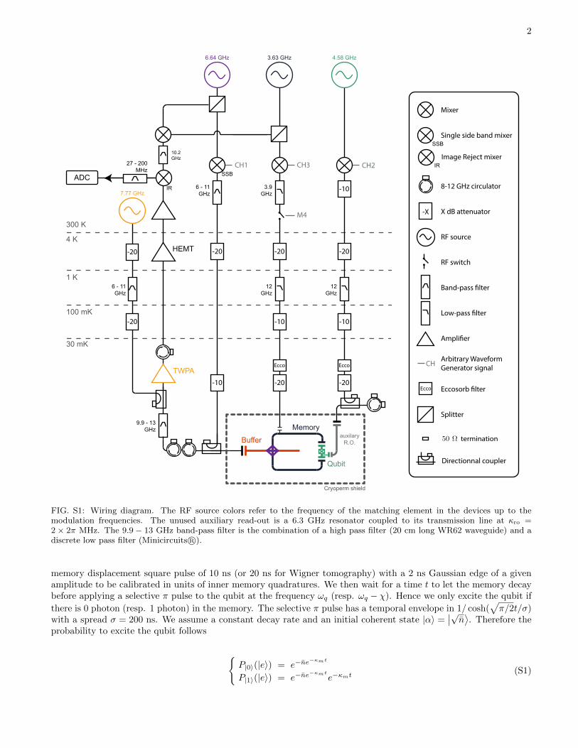
The sample is cooled down to T ≈ 30 mK in a BlueFors R©dilution refrigerator. The scheme of the microwave inputand output lines is provided in Fig. S1. The memory, pump and qubit pulses are generated by modulation of continuousmicrowave tones produced respectively by AnaPico R©(APSIN12G), Agilent R©(E8752D)and AnaPico R©(APSIN12G)sources set at the frequencies fm − 100 MHz, fb − fm + 150 MHz and fq + 128 MHz. The pump tone is modulatedthrough a single sideband mixer and the memory and qubit tones are modulated through regular mixers. Theparasitic sidebands at the output of the mixers are far detuned from any frequency of interest and are neglected.The RF modulation pulses are generated by a 4 channels Tektronix R©Abitrary Waveform Generator (AWG5014C)with a sample rate of 1 GS/s. Those pulses are of frequency 100 MHz, 150 MHz and 128 MHz. In order to ensurephase stability during the measurement, the local oscillator used for the demodulation of the output signal is notindependent from the other ones. It is generated by mixing the output of the two sources that are close to thememory and pump frequencies, followed by the filtering out of the lower sideband. We thus retrieve a tone atfrequency (fm − 100 MHz) + (fb − fm + 150 MHz) = fb + 50 MHz which is used to mix the signal down to 50 MHzbefore digitization.

The signal coming out of the buffer mode is filtered using a wave-guide with a cutoff frequency at 9.8 GHz inorder to protect the following amplification stage to be affected by the strong reflected pump tone. The signal is firstamplified by a Traveling Wave Parametric Amplifier (provided by W. Oliver group at Lincoln Labs). We tuned thepump frequency (fTWPA = 7.773 GHz) and power in order to reach a gain of 19 dB at 10.220 GHz. The followupamplification is performed by a High Electron Mobility Transistor (HEMT) amplifier (from Caltech) at 4 K and bytwo room temperature amplifiers.

Sample description

The sample was fabricated on a substrate of undoped Si (111) of dimension 8.67 × 8.16 × 0.28 mm. The groundplanes and resonators are made of 150 nm of sputtered Nb after HF treatment. An optical lithography is performedusing a laser writer before dry etching with SF6 the Nb layer. The Josephson junctions of the transmon and the JRMare fabricated using electronic lithography followed by an angle deposition of Al/AlOx/Al in a Plassys MEB550Sevaporator. A good contact between Al and Nb is ensured by ion milling the Nb oxide in the Plassys evaporator priorto the evaporation over the overlap pads of 50 × 50 µm2. The Nb sputtering was done in the Quantronics group atCEA Saclay, the wafer dicing at Observatoire de Paris, the Al evaporation in a Plassys R©ebeam evaporator and thelaser writing at College de France, the electronic lithography at ENS Paris and the HF treatment at Paris Diderot.All measurements were performed at ENS de Lyon.

The memory and the buffer are λ/2 resonators in coplanar waveguide architecture. They are coupled in theirmiddle by the JRM. The memory has a gap width of 50 µm and a central conductor width of 84 µm whereas thebuffer gap width is 10 µm and its central conductor width is 220 µm. This design is intended to minimize the buffercharacteristic impedance (here 25 Ω) in order to maximize the participation ratio of the JRM in that mode, withoutcompromising too much on the reproducibility of the fabrication. The memory is symmetrically coupled (see Fig. 1c)to the transmon qubit. Owing to this trick, the pump generates a negligible potential difference between the antennasof the Josephson Junction. This symmetric design reduces the coupling of the qubit to the pump drive by an estimated20 dB compared to an unpublished previous design (Fig. S2). This improvement was determined by measuring theminimal pump power that leads to ionization of the transmon [S1].

CALIBRATION

Memory quadrature and photon number calibration

The calibration of the memory quadratures in the Wigner functions and of the photon number in the memory weredone by monitoring the free temporal evolution of the occupations of the first Fock states. To do so, we apply a

2

9.9 - 13 GHz

auxilary R.O.

Qubit

Memory

Buffer

TWPA-10 -20 -20

Ecco Ecco

30 mK

100 mK-20 -10 -10

1 K

4 K-20

6 - 11 GHz

12 GHz

12 GHz

HEMT -20 -20-20

300 K

ADC IR

SSB

10.2GHz

3.9 GHz

CH3

M4

-10

CH227 - 200 MHz

CH1

6 - 11 GHz

8-12 GHz circulator

-X X dB attenuator

Band-pass lter

Low-pass lter

Ecco Eccosorb lter

Single side band mixer

Mixer

SSB

RF source

RF switch

Amplier

CHArbitrary Waveform Generator signal

Splitter

termination

Directionnal coupler

Cryoperm shield

Image Reject mixer IR

7.77 GHz

6.64 GHz 3.63 GHz 4.58 GHz

FIG. S1: Wiring diagram. The RF source colors refer to the frequency of the matching element in the devices up to themodulation frequencies. The unused auxiliary read-out is a 6.3 GHz resonator coupled to its transmission line at κro =2 × 2π MHz. The 9.9 − 13 GHz band-pass filter is the combination of a high pass filter (20 cm long WR62 waveguide) and adiscrete low pass filter (Minicircuits R©).

memory displacement square pulse of 10 ns (or 20 ns for Wigner tomography) with a 2 ns Gaussian edge of a givenamplitude to be calibrated in units of inner memory quadratures. We then wait for a time t to let the memory decaybefore applying a selective π pulse to the qubit at the frequency ωq (resp. ωq − χ). Hence we only excite the qubit if

there is 0 photon (resp. 1 photon) in the memory. The selective π pulse has a temporal envelope in 1/ cosh(√π/2t/σ)

with a spread σ = 200 ns. We assume a constant decay rate and an initial coherent state |α〉 =∣∣√n⟩. Therefore the

probability to excite the qubit follows

P|0〉(|e〉) = e−ne

−κmt

P|1〉(|e〉) = e−ne−κmt

e−κmt(S1)

3

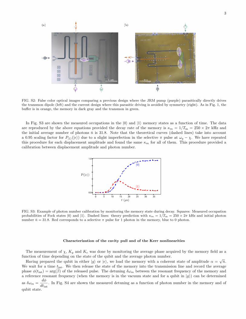
FIG. S2: False color optical images comparing a previous design where the JRM pump (purple) parasitically directly drivesthe transmon dipole (left) and the current design where this parasitic driving is avoided by symmetry (right). As in Fig. 1, thebuffer is in orange, the memory in dark gray and the transmon in green.

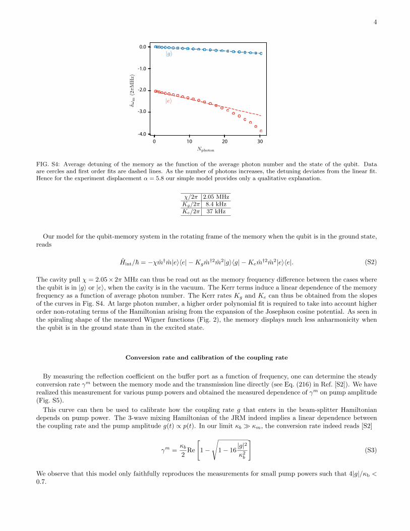
In Fig. S3 are shown the measured occupations in the |0〉 and |1〉 memory states as a function of time. The dataare reproduced by the above equations provided the decay rate of the memory is κm = 1/Tm = 250 × 2π kHz andthe initial average number of photons n is 31.8. Note that the theoretical curves (dashed lines) take into accounta 0.95 scaling factor for P|1〉(|e〉) due to a slight imperfection in the selective π pulse at ωq − χ. We have repeatedthis procedure for each displacement amplitude and found the same κm for all of them. This procedure provided acalibration between displacement amplitude and photon number.

1.0

0.0

0 5 10 15 20 25 30 35

FIG. S3: Example of photon number calibration by monitoring the memory state during decay. Squares: Measured occupationprobabilities of Fock states |0〉 and |1〉. Dashed lines: theory prediction with κm = 1/Tm = 250 × 2π kHz and initial photonnumber n = 31.8. Red corresponds to a selective π pulse for 1 photon in the memory, blue to 0 photon.

Characterization of the cavity pull and of the Kerr nonlinearities

The measurement of χ, Kg and Ke was done by monitoring the average phase acquired by the memory field as afunction of time depending on the state of the qubit and the average photon number.

Having prepared the qubit in either |g〉 or |e〉, we load the memory with a coherent state of amplitude α =√n.

We wait for a time tint. We then release the state of the memory into the transmission line and record the averagephase φ(tint) = arg(β) of the released pulse. The detuning δωm between the resonant frequency of the memory anda reference resonant frequency (when the memory is in the vacuum state and for a qubit in |g〉) can be determined

as δωm =dφ

dtint. In Fig. S4 are shown the measured detuning as a function of photon number in the memory and of

qubit state.

4

0 10 20 30

0.0

-1.0

-2.0

-3.0

-4.0

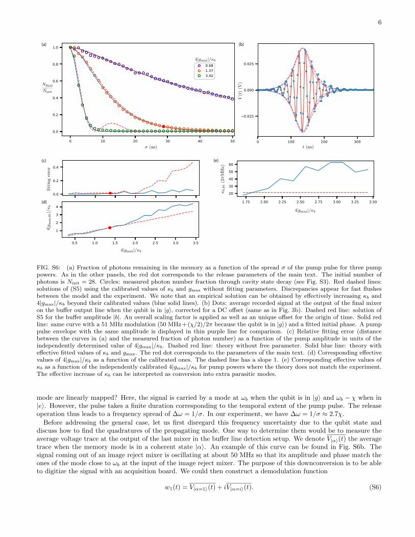
FIG. S4: Average detuning of the memory as the function of the average photon number and the state of the qubit. Dataare cercles and first order fits are dashed lines. As the number of photons increases, the detuning deviates from the linear fit.Hence for the experiment displacement α = 5.8 our simple model provides only a qualitative explanation.

χ/2π 2.05 MHzKg/2π 8.4 kHzKe/2π 37 kHz

Our model for the qubit-memory system in the rotating frame of the memory when the qubit is in the ground state,reads

Hint/~ = −χm†m|e〉〈e| −Kgm†2m2|g〉〈g| −Kem

†2m2|e〉〈e|. (S2)

The cavity pull χ = 2.05× 2π MHz can thus be read out as the memory frequency difference between the cases wherethe qubit is in |g〉 or |e〉, when the cavity is in the vacuum. The Kerr terms induce a linear dependence of the memoryfrequency as a function of average photon number. The Kerr rates Kg and Ke can thus be obtained from the slopesof the curves in Fig. S4. At large photon number, a higher order polynomial fit is required to take into account higherorder non-rotating terms of the Hamiltonian arising from the expansion of the Josephson cosine potential. As seen inthe spiraling shape of the measured Wigner functions (Fig. 2), the memory displays much less anharmonicity whenthe qubit is in the ground state than in the excited state.

Conversion rate and calibration of the coupling rate

By measuring the reflection coefficient on the buffer port as a function of frequency, one can determine the steadyconversion rate γm between the memory mode and the transmission line directly (see Eq. (216) in Ref. [S2]). We haverealized this measurement for various pump powers and obtained the measured dependence of γm on pump amplitude(Fig. S5).

This curve can then be used to calibrate how the coupling rate g that enters in the beam-splitter Hamiltoniandepends on pump power. The 3-wave mixing Hamiltonian of the JRM indeed implies a linear dependence betweenthe coupling rate and the pump amplitude g(t) ∝ p(t). In our limit κb κm, the conversion rate indeed reads [S2]

γm =κb2

Re

[1−

√1− 16

|g|2κ2b

](S3)

We observe that this model only faithfully reproduces the measurements for small pump powers such that 4|g|/κb <0.7.

5

(a) (b) (c) (d)

FIG. S5: (a) Direct coupling measurement (purple square) to the memory as a function of the pump amplitude. We obtainthe calibration for the coupling g from the fit (dashed gray line). (b) to (d) Blue solid line : phase of the measured reflectioncoefficient on the buffer port for various pump amplitudes. Red dashed line : corresponding curve obtained by tuning γm,which allows us to plot one dot in (a). The color of each frame corresponds to the color of its corresponding dot in figure (a).

Dynamics of the memory release

The flushing of the memory by the smooth pump pulse is characterized as follows. The memory is loaded with acoherent state with amplitude α = 5.3. In the following the qubit is assumed to be in its ground state[S11]. It isjustified by the fact that χ κb, for which the release dynamics is similar for the qubit in the ground or in the excited

state. A pump pulse with an envelope p(t) ∝(

cosh (√π/2t/σ)

)−1

is applied for various pump amplitudes and spread

(Fig. S6). This choice of a smooth pump pulse allows us to limit the spectral broadening of the pump. The Fouriertransform of that pulse has the same shape but with a variance 1/σ. In practice, the pump pulse is windowed bya square shaped weight function of duration 8σ. We then measure the remaining average photon number using thetechnique of cavity state decay as in Fig. S3.

The release dynamics is captured by the quantum Langevin equation for the field amplitudes m and b in the rotatingframes of the buffer and the memory.

m = −ig?b− κm

2 m

b = −igm− κb2 b

(S4)

Hence,

m+

(κb2 + κm

2 −g?

g?

)m+

(|g|2 + κmκb

4 − κm2g∗

g∗

)m = 0

g?b− i(m+ κm

2 m)

= 0(S5)

with g(t) = gmax/ cosh(√

π/2t/σ)

and g?

g? (t) = −√π/2 tanh

(√π/2t/σ

)σ .

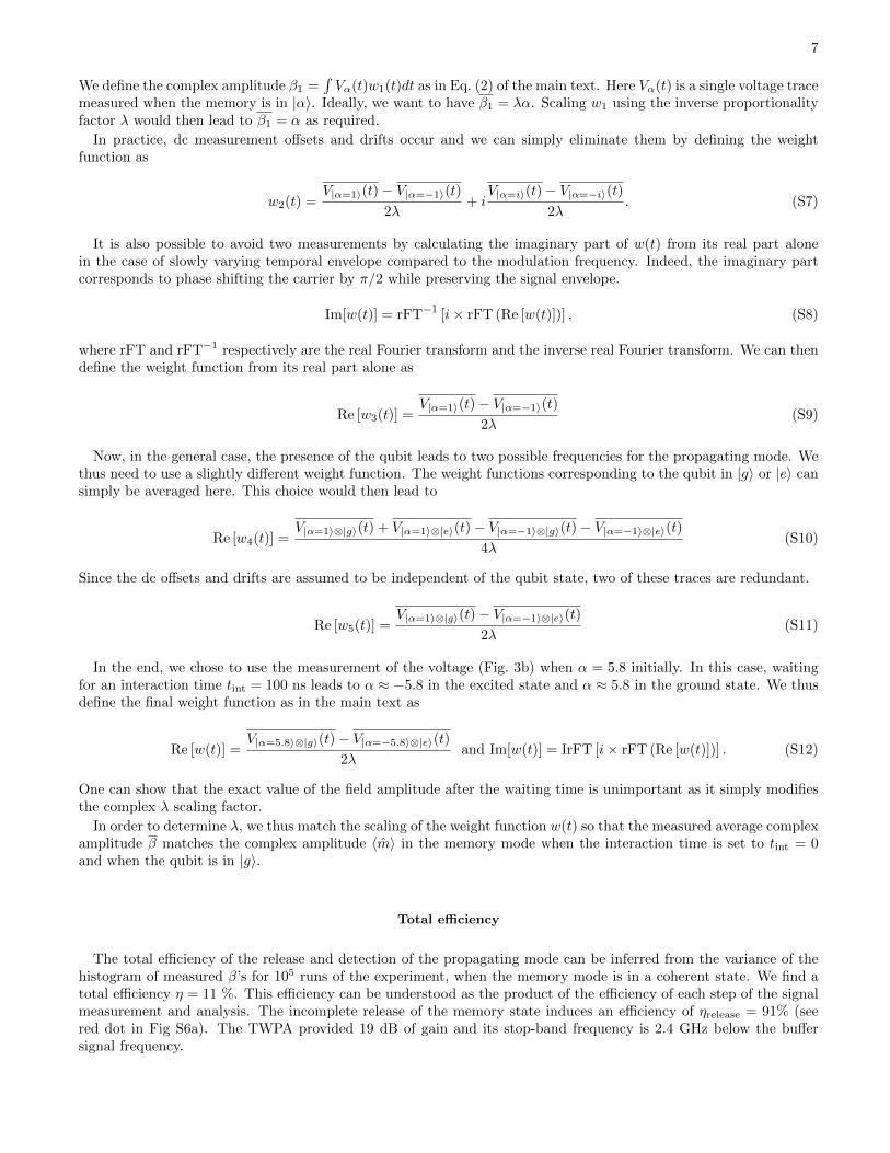
In Fig. S6a are shown the measured memory photon number normalized to the initial number as a function of σand for various pump powers. The numerical solution of the above equation reproduces well these measurements aslong as 4|gmax|/κb does not exceed 1.6 (Fig. S6c). There, even the average time trace of the buffer output is wellcaptured (Fig. S6b).

For the largest pump powers, for which this value is exceeded, the memory is flushed more rapidly than theoreticallyexpected. The observed behavior can be captured by allowing to tune the effective values of κb and gmax. The increaseof the effective decay rate κb could be due to the conversion of the memory mode into parasitic unmonitored modes(Fig. S6e).

SIGNAL PROCESSING

Demodulation basis construction

As the memory mode is released into the buffer line, its quantum state is mapped into a propagating microwavemode. How to determine the quadratures of the propagating mode into which the quadratures of the inner memory

6

(a) (b)

(c) (e)

(d)

FIG. S6: (a) Fraction of photons remaining in the memory as a function of the spread σ of the pump pulse for three pumppowers. As in the other panels, the red dot corresponds to the release parameters of the main text. The initial number ofphotons is Ninit = 28. Circles: measured photon number fraction through cavity state decay (see Fig. S3). Red dashed lines:solutions of (S5) using the calibrated values of κb and gmax without fitting parameters. Discrepancies appear for fast flushesbetween the model and the experiment. We note that an empirical solution can be obtained by effectively increasing κb and4|gmax|/κb beyond their calibrated values (blue solid lines). (b) Dots: average recorded signal at the output of the final mixeron the buffer output line when the qubit is in |g〉, corrected for a DC offset (same as in Fig. 3b). Dashed red line: solution ofS5 for the buffer amplitude |b|. An overall scaling factor is applied as well as an unique offset for the origin of time. Solid redline: same curve with a 51 MHz modulation (50 MHz+(χ/2)/2π because the qubit is in |g〉) and a fitted initial phase. A pumppulse envelope with the same amplitude is displayed in thin purple line for comparison. (c) Relative fitting error (distancebetween the curves in (a) and the measured fraction of photon number) as a function of the pump amplitude in units of theindependently determined value of 4|gmax|/κb. Dashed red line: theory without free parameter. Solid blue line: theory witheffective fitted values of κb and gmax. The red dot corresponds to the parameters of the main text. (d) Corresponding effectivevalues of 4|gmax|/κb as a function of the calibrated ones. The dashed line has a slope 1. (e) Corresponding effective values ofκb as a function of the independently calibrated 4|gmax|/κb for pump powers where the theory does not match the experiment.The effective increase of κb can be interpreted as conversion into extra parasitic modes.

mode are linearly mapped? Here, the signal is carried by a mode at ωb when the qubit is in |g〉 and ωb − χ when in|e〉. However, the pulse takes a finite duration corresponding to the temporal extent of the pump pulse. The releaseoperation thus leads to a frequency spread of ∆ω = 1/σ. In our experiment, we have ∆ω = 1/σ ≈ 2.7χ.

Before addressing the general case, let us first disregard this frequency uncertainty due to the qubit state anddiscuss how to find the quadratures of the propagating mode. One way to determine them would be to measure theaverage voltage trace at the output of the last mixer in the buffer line detection setup. We denote V|α〉(t) the averagetrace when the memory mode is in a coherent state |α〉. An example of this curve can be found in Fig. S6b. Thesignal coming out of an image reject mixer is oscillating at about 50 MHz so that its amplitude and phase match theones of the mode close to ωb at the input of the image reject mixer. The purpose of this downconversion is to be ableto digitize the signal with an acquisition board. We could then construct a demodulation function

w1(t) = V|α=1〉(t) + iV|α=i〉(t). (S6)

7

We define the complex amplitude β1 =∫Vα(t)w1(t)dt as in Eq. (2) of the main text. Here Vα(t) is a single voltage trace

measured when the memory is in |α〉. Ideally, we want to have β1 = λα. Scaling w1 using the inverse proportionalityfactor λ would then lead to β1 = α as required.

In practice, dc measurement offsets and drifts occur and we can simply eliminate them by defining the weightfunction as

w2(t) =V|α=1〉(t)− V|α=−1〉(t)

2λ+ i

V|α=i〉(t)− V|α=−i〉(t)

2λ. (S7)

It is also possible to avoid two measurements by calculating the imaginary part of w(t) from its real part alonein the case of slowly varying temporal envelope compared to the modulation frequency. Indeed, the imaginary partcorresponds to phase shifting the carrier by π/2 while preserving the signal envelope.

Im[w(t)] = rFT−1 [i× rFT (Re [w(t)])] , (S8)

where rFT and rFT−1 respectively are the real Fourier transform and the inverse real Fourier transform. We can thendefine the weight function from its real part alone as

Re [w3(t)] =V|α=1〉(t)− V|α=−1〉(t)

2λ(S9)

Now, in the general case, the presence of the qubit leads to two possible frequencies for the propagating mode. Wethus need to use a slightly different weight function. The weight functions corresponding to the qubit in |g〉 or |e〉 cansimply be averaged here. This choice would then lead to

Re [w4(t)] =V|α=1〉⊗|g〉(t) + V|α=1〉⊗|e〉(t)− V|α=−1〉⊗|g〉(t)− V|α=−1〉⊗|e〉(t)

4λ(S10)

Since the dc offsets and drifts are assumed to be independent of the qubit state, two of these traces are redundant.

Re [w5(t)] =V|α=1〉⊗|g〉(t)− V|α=−1〉⊗|e〉(t)

2λ(S11)

In the end, we chose to use the measurement of the voltage (Fig. 3b) when α = 5.8 initially. In this case, waitingfor an interaction time tint = 100 ns leads to α ≈ −5.8 in the excited state and α ≈ 5.8 in the ground state. We thusdefine the final weight function as in the main text as

Re [w(t)] =V|α=5.8〉⊗|g〉(t)− V|α=−5.8〉⊗|e〉(t)

2λand Im[w(t)] = IrFT [i× rFT (Re [w(t)])] . (S12)

One can show that the exact value of the field amplitude after the waiting time is unimportant as it simply modifiesthe complex λ scaling factor.

In order to determine λ, we thus match the scaling of the weight function w(t) so that the measured average complexamplitude β matches the complex amplitude 〈m〉 in the memory mode when the interaction time is set to tint = 0and when the qubit is in |g〉.

Total efficiency

The total efficiency of the release and detection of the propagating mode can be inferred from the variance of thehistogram of measured β’s for 105 runs of the experiment, when the memory mode is in a coherent state. We find atotal efficiency η = 11 %. This efficiency can be understood as the product of the efficiency of each step of the signalmeasurement and analysis. The incomplete release of the memory state induces an efficiency of ηrelease = 91% (seered dot in Fig S6a). The TWPA provided 19 dB of gain and its stop-band frequency is 2.4 GHz below the buffersignal frequency.

8

CHOICE OF PARAMETERS

Optimal release amplitude and temporal envelope

The goal of this experiment is to demonstrate a sequential single shot read-out with the highest achievable fidelity.We chose the optimal parameters by minimizing the overlap between the distribution P|e〉 and P|g〉. The pumptemporal shape was chosen to minimize this overlap. There is a trade-off between the speed of the flush and themeasurement fidelity. Indeed, a fast flush reduces the efficiency as it dissipates a fraction of the memory energy inunmonitored modes (see Fig. S6). On the other hand, a slower flush is not able to release the probe when it is at themaximum phase difference. Instead, it continuously releases the probe signal as it interacts with the qubit.

In our experiment, this trade-off yields an optimal pump spread σ = 28 ns and maximum coupling |gmax| =7.2× 2π MHz > κb

4 corresponding to a slight over-critical coupling of the memory and the buffer.

Operating flux bias of the JRM

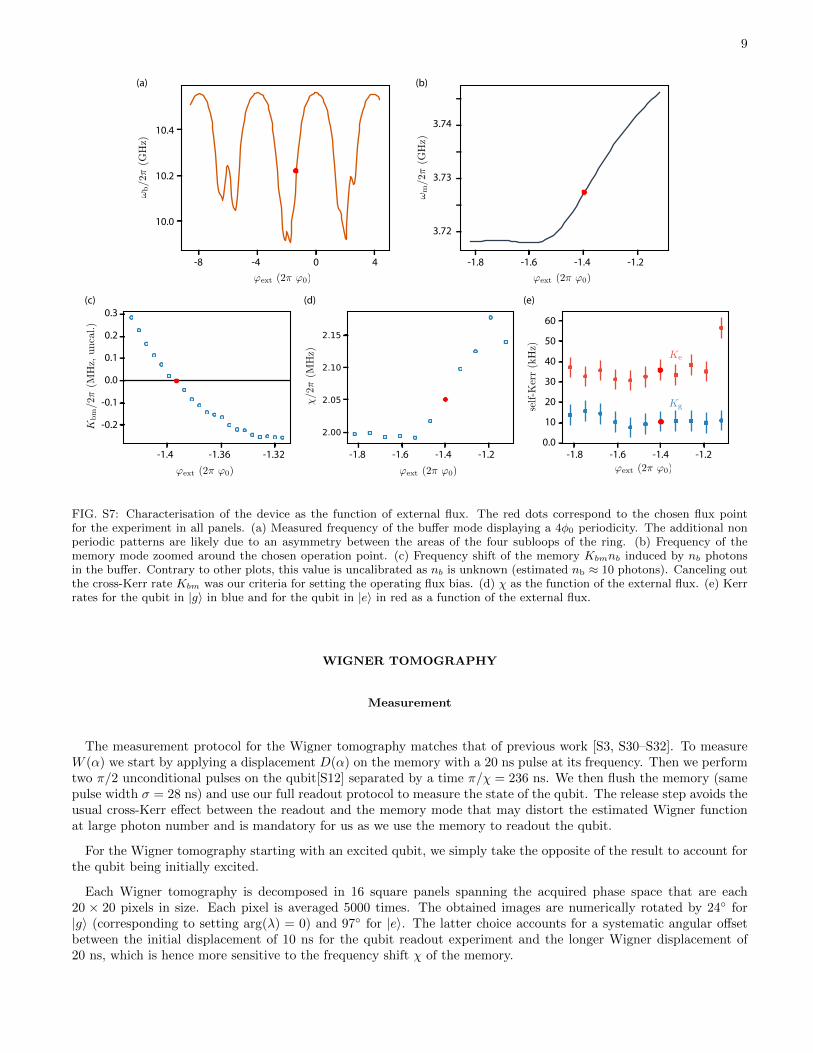
The behaviour of the shunted JRM as a function of the external flux was studied in depth in previous works [S2].By measuring the reflection coefficient on the buffer port, we determined the buffer frequency as a function of theexternal magnetic flux (Fig. S7a).

We then characterize the cross-Kerr effect induced by the buffer occupation on the memory. To do so, we displacethe memory with α0 ≈ 5. Then we apply a continuous tone at the buffer frequency on the buffer port for a timet corresponding to an estimated 10 photons in the buffer at the end of the pulse, which is large compare to 1/κb.Finally we release the memory state into the buffer and measure its average phase arg(β). The acquired phase as afunction of time t provides us the memory frequency (as in Fig. S4). We subtract to this measured frequency the onemeasured without driving the buffer and obtain a measurement of the modification of the memory frequency by thebuffer occupation without any calibration of the buffer photon number at this stage. This cross-Kerr effect cancelsout for a given value of the external flux as expected for the JRM. We chose this flux point for the experiment as itensures that the memory is decoupled from the transmission line during the interaction time and as it also cancels outthe cross-Kerr effect induced by the pump tone during the release. We use the same method as in Fig. S4 to measurethe self-Kerr rate and χ as a function of the external flux. The self-Kerr rate is dominated by the contribution of thesingle junction transmon qubit and hence show little to no flux dependency. Increasing the JRM participation ratioshould increase this Kerr tunability by the flux and enables a canceling of the average Kerr in the memory mode.

9

10.4

10.0

10.2

-8 -4 0 4 -1.8 -1.6 -1.4 -1.2

3.74

3.72

3.73

-1.8 -1.6 -1.4 -1.2 -1.8 -1.6 -1.4 -1.20.0

10

20

30

40

50

60

-1.4 -1.36 -1.32

-0.2

-0.1

0.0

0.1

0.2

0.3

(a) (b)

(c) (d) (e)

FIG. S7: Characterisation of the device as the function of external flux. The red dots correspond to the chosen flux pointfor the experiment in all panels. (a) Measured frequency of the buffer mode displaying a 4φ0 periodicity. The additional nonperiodic patterns are likely due to an asymmetry between the areas of the four subloops of the ring. (b) Frequency of thememory mode zoomed around the chosen operation point. (c) Frequency shift of the memory Kbmnb induced by nb photonsin the buffer. Contrary to other plots, this value is uncalibrated as nb is unknown (estimated nb ≈ 10 photons). Canceling outthe cross-Kerr rate Kbm was our criteria for setting the operating flux bias. (d) χ as the function of the external flux. (e) Kerrrates for the qubit in |g〉 in blue and for the qubit in |e〉 in red as a function of the external flux.

WIGNER TOMOGRAPHY

Measurement

The measurement protocol for the Wigner tomography matches that of previous work [S3, S30–S32]. To measureW (α) we start by applying a displacement D(α) on the memory with a 20 ns pulse at its frequency. Then we performtwo π/2 unconditional pulses on the qubit[S12] separated by a time π/χ = 236 ns. We then flush the memory (samepulse width σ = 28 ns) and use our full readout protocol to measure the state of the qubit. The release step avoids theusual cross-Kerr effect between the readout and the memory mode that may distort the estimated Wigner functionat large photon number and is mandatory for us as we use the memory to readout the qubit.

For the Wigner tomography starting with an excited qubit, we simply take the opposite of the result to account forthe qubit being initially excited.

Each Wigner tomography is decomposed in 16 square panels spanning the acquired phase space that are each20 × 20 pixels in size. Each pixel is averaged 5000 times. The obtained images are numerically rotated by 24 for|g〉 (corresponding to setting arg(λ) = 0) and 97 for |e〉. The latter choice accounts for a systematic angular offsetbetween the initial displacement of 10 ns for the qubit readout experiment and the longer Wigner displacement of20 ns, which is hence more sensitive to the frequency shift χ of the memory.

10

Qubit prepared in Qubit prepared in

SimulationExperiment SimulationExperimentTime

0.0

0.0

7.0

7.0

-7.0

-7.0

-0.2

0.0

1.0

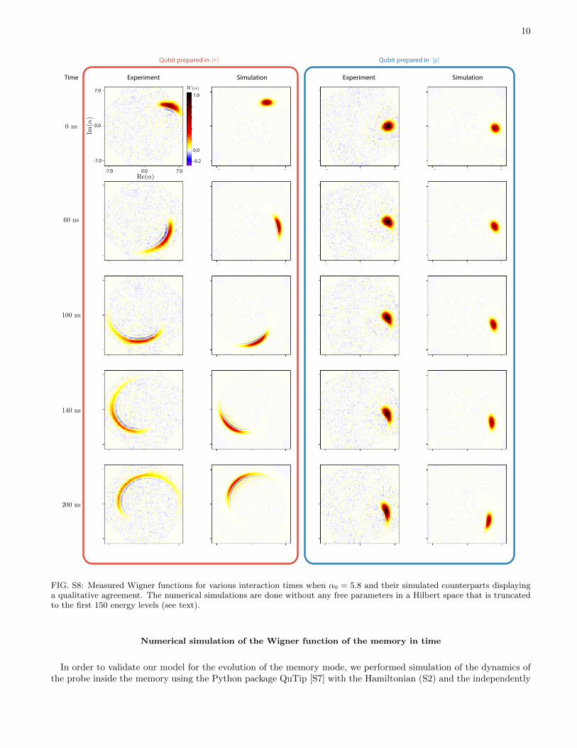
FIG. S8: Measured Wigner functions for various interaction times when α0 = 5.8 and their simulated counterparts displayinga qualitative agreement. The numerical simulations are done without any free parameters in a Hilbert space that is truncatedto the first 150 energy levels (see text).

Numerical simulation of the Wigner function of the memory in time

In order to validate our model for the evolution of the memory mode, we performed simulation of the dynamics ofthe probe inside the memory using the Python package QuTip [S7] with the Hamiltonian (S2) and the independently

11

measured values for its parameters (see above sections). The fit includes an extra 20 ns delay to account for theduration of the displacement pulse. The results are provided on Fig. S8 and display a qualitative agreement withthe measurement. It confirms that the probe state dynamics is mainly governed by the χ and Kerr terms of theHamiltonian.

READOUT CHARACTERIZATION

Measurement fidelity

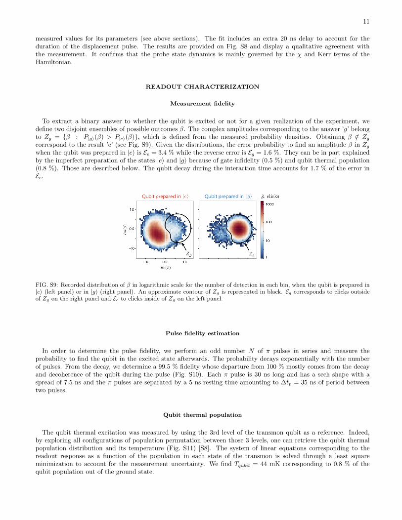
To extract a binary answer to whether the qubit is excited or not for a given realization of the experiment, wedefine two disjoint ensembles of possible outcomes β. The complex amplitudes corresponding to the answer ’g’ belongto Zg = β : P|g〉(β) > P|e〉(β), which is defined from the measured probability densities. Obtaining β /∈ Zgcorrespond to the result ’e’ (see Fig. S9). Given the distributions, the error probability to find an amplitude β in Zgwhen the qubit was prepared in |e〉 is Ee = 3.4 % while the reverse error is Eg = 1.6 %. They can be in part explainedby the imperfect preparation of the states |e〉 and |g〉 because of gate infidelity (0.5 %) and qubit thermal population(0.8 %). Those are described below. The qubit decay during the interaction time accounts for 1.7 % of the error inEe.

FIG. S9: Recorded distribution of β in logarithmic scale for the number of detection in each bin, when the qubit is prepared in|e〉 (left panel) or in |g〉 (right panel). An approximate contour of Zg is represented in black. Eg corresponds to clicks outsideof Zg on the right panel and Ee to clicks inside of Zg on the left panel.

Pulse fidelity estimation

In order to determine the pulse fidelity, we perform an odd number N of π pulses in series and measure theprobability to find the qubit in the excited state afterwards. The probability decays exponentially with the numberof pulses. From the decay, we determine a 99.5 % fidelity whose departure from 100 % mostly comes from the decayand decoherence of the qubit during the pulse (Fig. S10). Each π pulse is 30 ns long and has a sech shape with aspread of 7.5 ns and the π pulses are separated by a 5 ns resting time amounting to ∆tp = 35 ns of period betweentwo pulses.

Qubit thermal population

The qubit thermal excitation was measured by using the 3rd level of the transmon qubit as a reference. Indeed,by exploring all configurations of population permutation between those 3 levels, one can retrieve the qubit thermalpopulation distribution and its temperature (Fig. S11) [S8]. The system of linear equations corresponding to thereadout response as a function of the population in each state of the transmon is solved through a least squareminimization to account for the measurement uncertainty. We find Tqubit = 44 mK corresponding to 0.8 % of thequbit population out of the ground state.

12

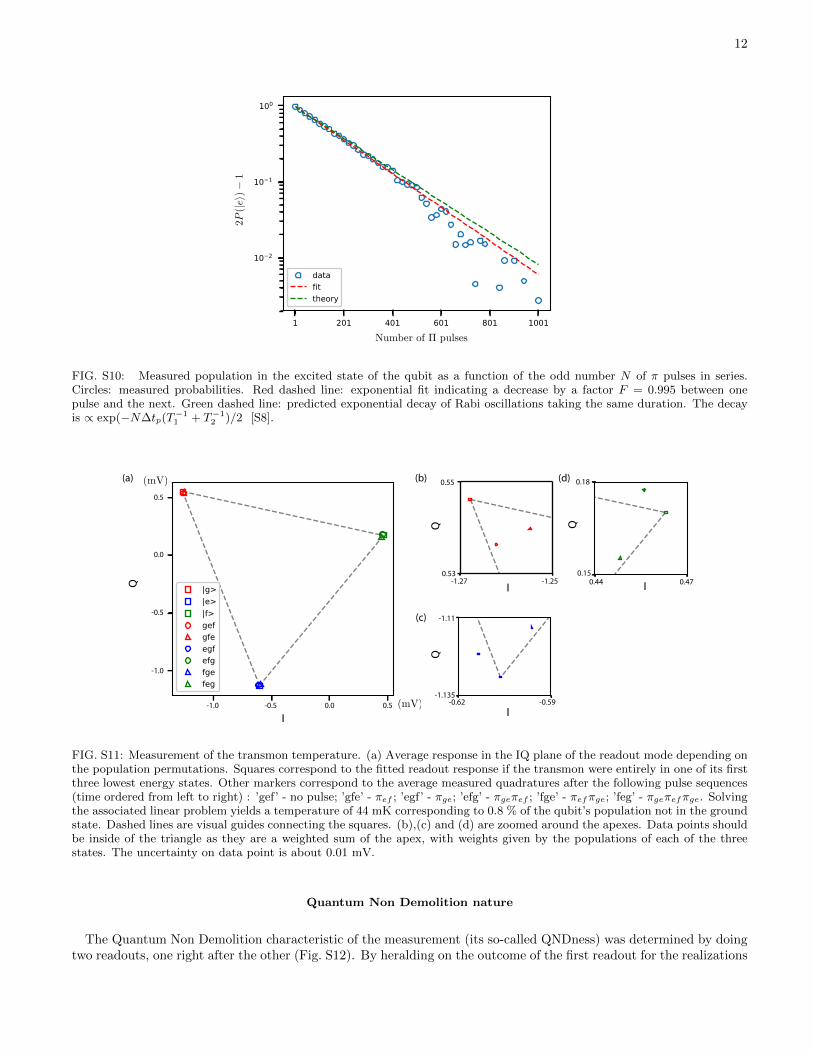
FIG. S10: Measured population in the excited state of the qubit as a function of the odd number N of π pulses in series.Circles: measured probabilities. Red dashed line: exponential fit indicating a decrease by a factor F = 0.995 between onepulse and the next. Green dashed line: predicted exponential decay of Rabi oscillations taking the same duration. The decayis ∝ exp(−N∆tp(T−1

1 + T−12 )/2 [S8].

0.0

0.5

-0.5

-1.0

0.0 0.5-1.0 -0.5

0.55

0.53-1.27 -1.25

-1.11

-1.135-0.62 -0.59

0.18

0.150.470.44

(a) (b)

(c)

(d)

FIG. S11: Measurement of the transmon temperature. (a) Average response in the IQ plane of the readout mode depending onthe population permutations. Squares correspond to the fitted readout response if the transmon were entirely in one of its firstthree lowest energy states. Other markers correspond to the average measured quadratures after the following pulse sequences(time ordered from left to right) : ’gef’ - no pulse; ’gfe’ - πef ; ’egf’ - πge; ’efg’ - πgeπef ; ’fge’ - πefπge; ’feg’ - πgeπefπge. Solvingthe associated linear problem yields a temperature of 44 mK corresponding to 0.8 % of the qubit’s population not in the groundstate. Dashed lines are visual guides connecting the squares. (b),(c) and (d) are zoomed around the apexes. Data points shouldbe inside of the triangle as they are a weighted sum of the apex, with weights given by the populations of each of the threestates. The uncertainty on data point is about 0.01 mV.

Quantum Non Demolition nature

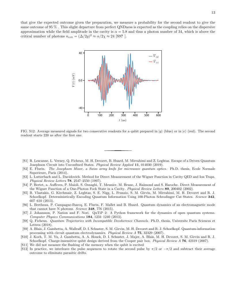
The Quantum Non Demolition characteristic of the measurement (its so-called QNDness) was determined by doingtwo readouts, one right after the other (Fig. S12). By heralding on the outcome of the first readout for the realizations

13

that give the expected outcome given the preparation, we measure a probability for the second readout to give thesame outcome of 95 % . This slight departure from perfect QNDness is expected as the coupling relies on the dispersiveapproximation while the field amplitude in the cavity is α = 5.8 and thus a photon number of 34, which is above thecritical number of photons ncrit = (∆/2g)2 ≈ α/2χ ≈ 24 [S9? ].

40

0.0

-40

0 100 200 300 400 500 600

FIG. S12: Average measured signals for two consecutive readouts for a qubit prepared in |g〉 (blue) or in |e〉 (red). The secondreadout starts 220 ns after the first one.

[S1] R. Lescanne, L. Verney, Q. Ficheux, M. H. Devoret, B. Huard, M. Mirrahimi and Z. Leghtas. Escape of a Driven QuantumJosephson Circuit into Unconfined States. Physical Review Applied 11, 014030 (2019).

[S2] E. Flurin. The Josephson Mixer, a Swiss army knife for microwave quantum optics. Ph.D. thesis, Ecole NormaleSuperieure, Paris (2014).

[S3] L. Lutterbach and L. Davidovich. Method for Direct Measurement of the Wigner Function in Cavity QED and Ion Traps.Physical Review Letters 78, 2547–2550 (1997).

[S4] P. Bertet, a. Auffeves, P. Maioli, S. Osnaghi, T. Meunier, M. Brune, J. Raimond and S. Haroche. Direct Measurement ofthe Wigner Function of a One-Photon Fock State in a Cavity. Physical Review Letters 89, 200402 (2002).

[S5] B. Vlastakis, G. Kirchmair, Z. Leghtas, S. E. Nigg, L. Frunzio, S. M. Girvin, M. Mirrahimi, M. H. Devoret and R. J.Schoelkopf. Deterministically Encoding Quantum Information Using 100-Photon Schrodinger Cat States. Science 342,607–610 (2013).

[S6] L. Bretheau, P. Campagne-Ibarcq, E. Flurin, F. Mallet and B. Huard. Quantum dynamics of an electromagnetic modethat cannot have N photons. Science 348, 776 (2015).

[S7] J. Johansson, P. Nation and F. Nori. QuTiP 2: A Python framework for the dynamics of open quantum systems.Computer Physics Communications 184, 1234–1240 (2013).

[S8] Q. Ficheux. Quantum Trajectories with Incompatible Decoherence Channels. Ph.D. thesis, Universite Paris Sciences etLettres (2018).

[S9] A. Blais, J. Gambetta, A. Wallraff, D. I. Schuster, S. M. Girvin, M. H. Devoret and R. J. Schoelkopf. Quantum-informationprocessing with circuit quantum electrodynamics. Physical Review A 75, 32329 (2007).

[S10] J. Koch, T. M. Yu, J. Gambetta, A. A. Houck, D. I. Schuster, J. Majer, A. Blais, M. H. Devoret, S. M. Girvin and R. J.Schoelkopf. Charge-insensitive qubit design derived from the Cooper pair box. Physical Review A 76, 42319 (2007).

[S11] We did not measure the flushing of the memory when the qubit is excited[S12] In practice, we interleave the pulse sequences to rotate the second pulse by π/2 or −π/2 and subtract their average

outcome to eliminate parasitic drifts.