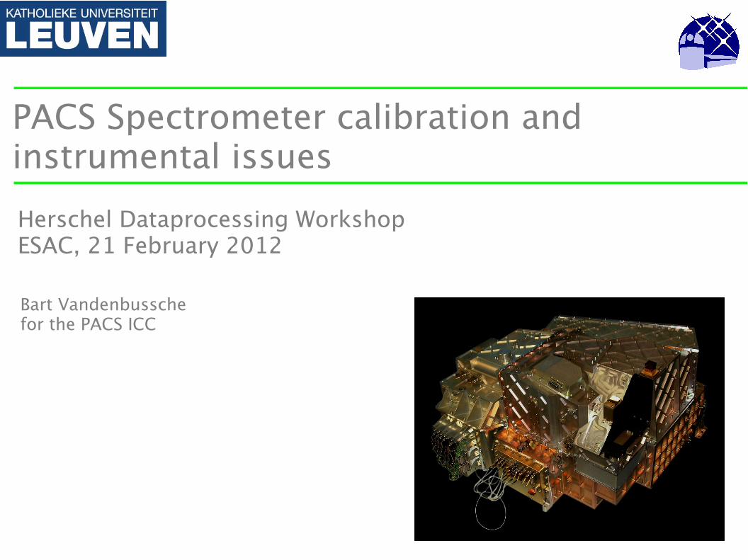
PACS Spectrometer calibration and instrumental issues

Bart Vandenbussche for the PACS ICC

Herschel Dataprocessing WorkshopESAC, 21 February 2012

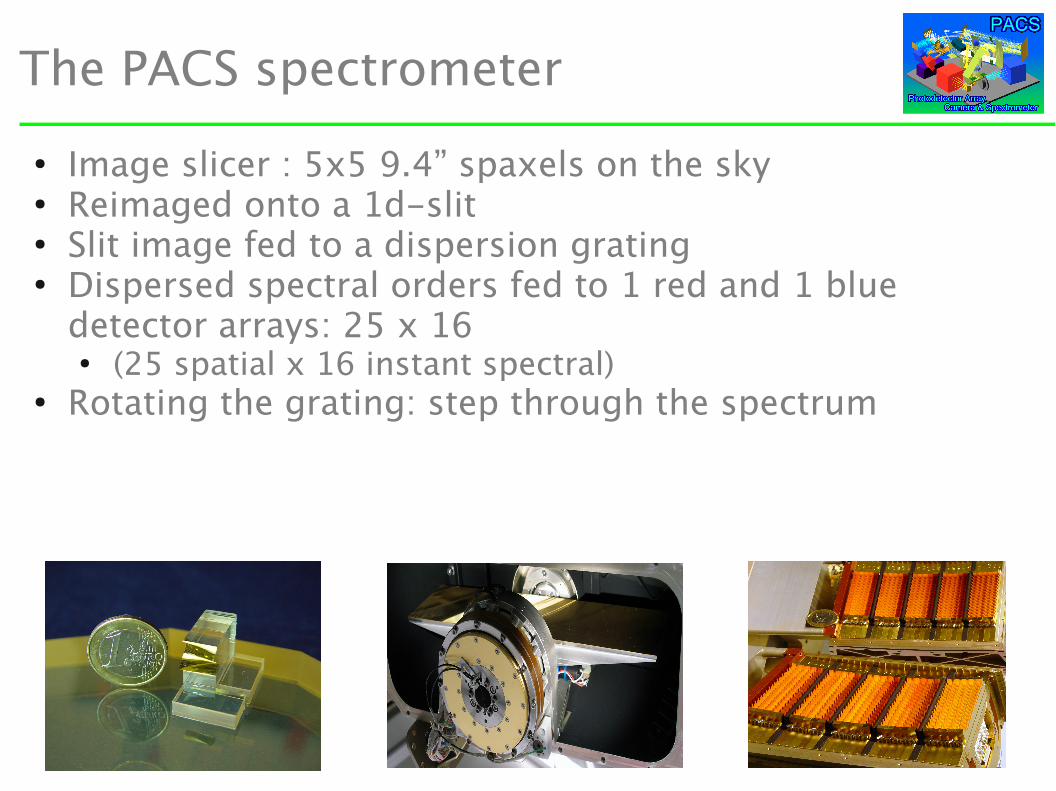
The PACS spectrometer

● Image slicer : 5x5 9.4” spaxels on the sky● Reimaged onto a 1d-slit● Slit image fed to a dispersion grating● Dispersed spectral orders fed to 1 red and 1 blue

detector arrays: 25 x 16 ● (25 spatial x 16 instant spectral)

● Rotating the grating: step through the spectrum

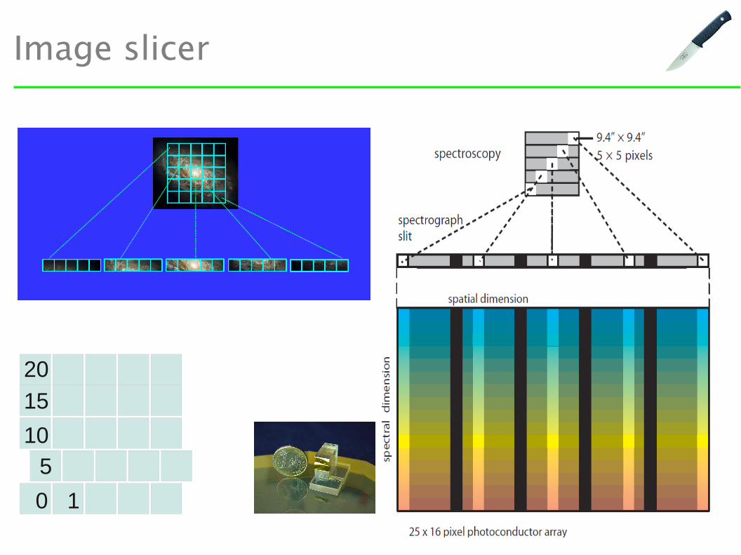
Image slicer

105

15

20

0 1

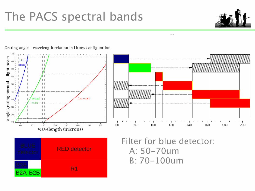
The PACS spectral bands

Filter for blue detector: A: 50-70um B: 70-100um

RED detectorBLUE

detector

B3AB2A B2B

R1

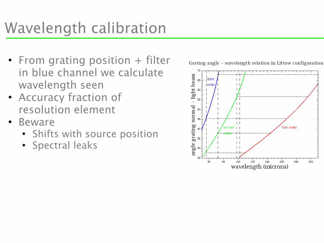
Wavelength calibration

● From grating position + filter in blue channel we calculate wavelength seen

● Accuracy fraction of resolution element

● Beware● Shifts with source position● Spectral leaks

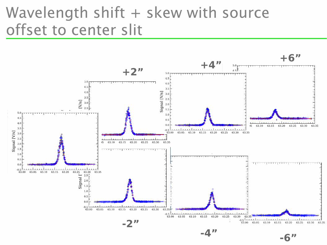
Wavelength shift + skew with source offset to center slit

-2”

+2”+4”

-4” -6”

+6”

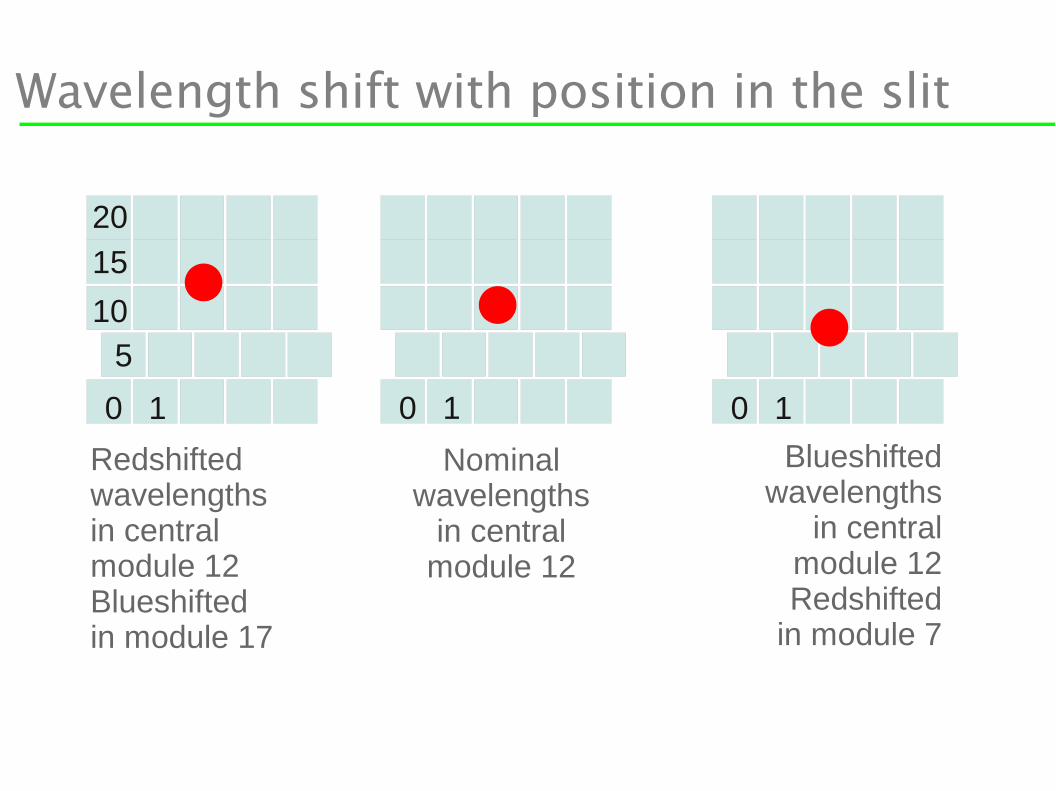
Wavelength shift with position in the slit

2” red dash, 1.5” black dash, slit border solid red

Wavelength shift with position in the slit

0 1 0 10 1

10

Nominal wavelengths

in central module 12

Redshifted wavelengthsin central module 12Blueshiftedin module 17

5

15

20

Blueshifted wavelengths

in central module 12Redshifted

in module 7

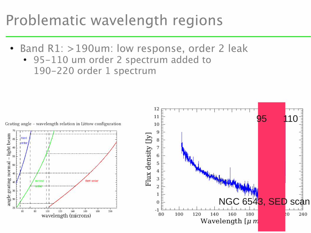
Problematic wavelength regions

● Band R1: >190um: low response, order 2 leak ● 95-110 um order 2 spectrum added to

190-220 order 1 spectrum

95 110

NGC 6543, SED scan

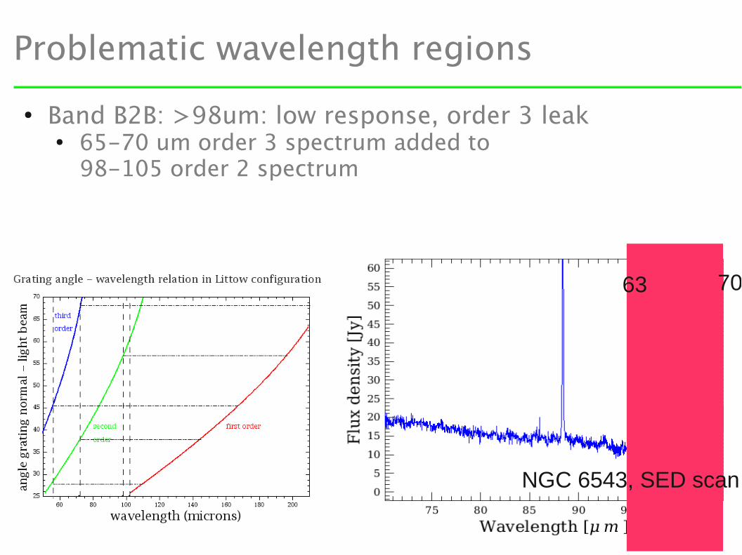
Problematic wavelength regions

● Band B2B: >98um: low response, order 3 leak ● 65-70 um order 3 spectrum added to

98-105 order 2 spectrum

63 70

NGC 6543, SED scan

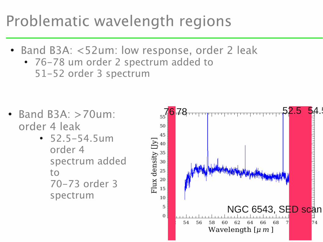
Problematic wavelength regions

● Band B3A: <52um: low response, order 2 leak ● 76-78 um order 2 spectrum added to

51-52 order 3 spectrum

76 78● Band B3A: >70um: order 4 leak

● 52.5-54.5um order 4 spectrum added to 70-73 order 3 spectrum

52.5 54.5

NGC 6543, SED scan

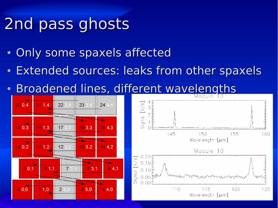
2nd pass ghosts2nd pass ghosts

● Only some spaxels affectedOnly some spaxels affected● Extended sources: leaks from other spaxelsExtended sources: leaks from other spaxels● Broadened lines, different wavelengths Broadened lines, different wavelengths

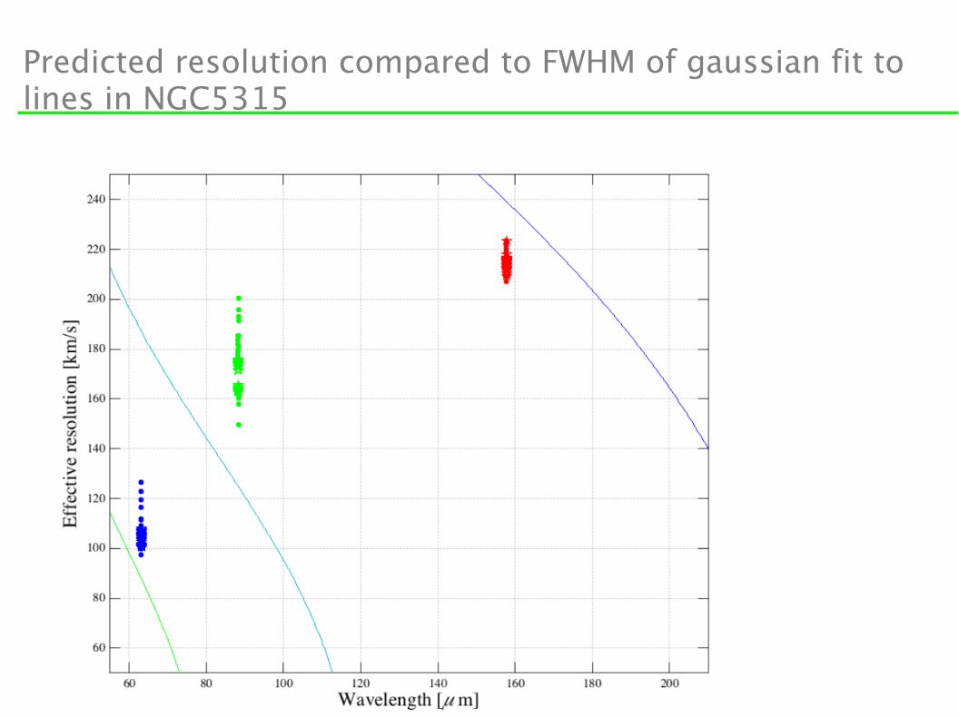
Predicted resolution compared to FWHM of gaussian fit to lines in NGC5315

PACS flux calibration concepts

● Nominal response + Relative Spectral Response (RSRF)● Average response spaxel 2,2 from sky calibrator obs● Flatfield from telescope background● RSRF from ILT

● Response from internal calibration block + RSRF● Internal calibration block: differential signal hot/cold load● Internal calibration block calibrated on sky calibrators● Flatfield from telescope background● RSRF from ILT

● Telescope normalisation for chopped measurements● E(source)/E(Telescope) ● E(Telescope) calibrated on Neptune raster

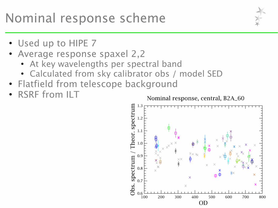
Nominal response scheme

● Used up to HIPE 7● Average response spaxel 2,2

● At key wavelengths per spectral band● Calculated from sky calibrator obs / model SED

● Flatfield from telescope background● RSRF from ILT

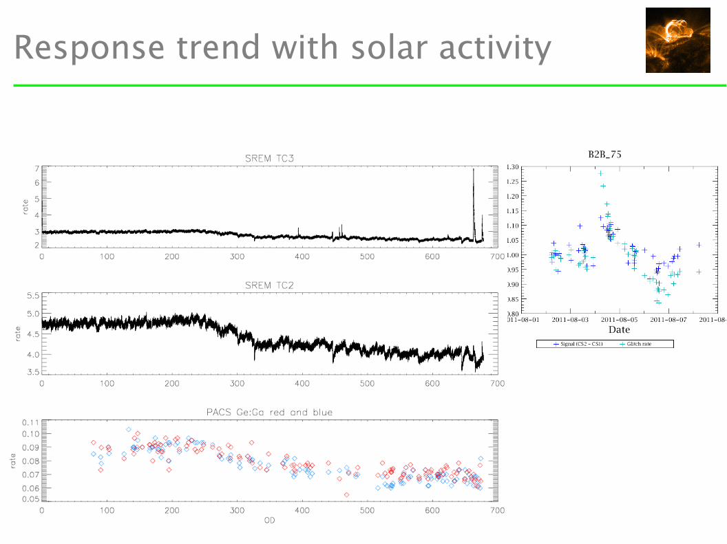
Response trend with solar activity

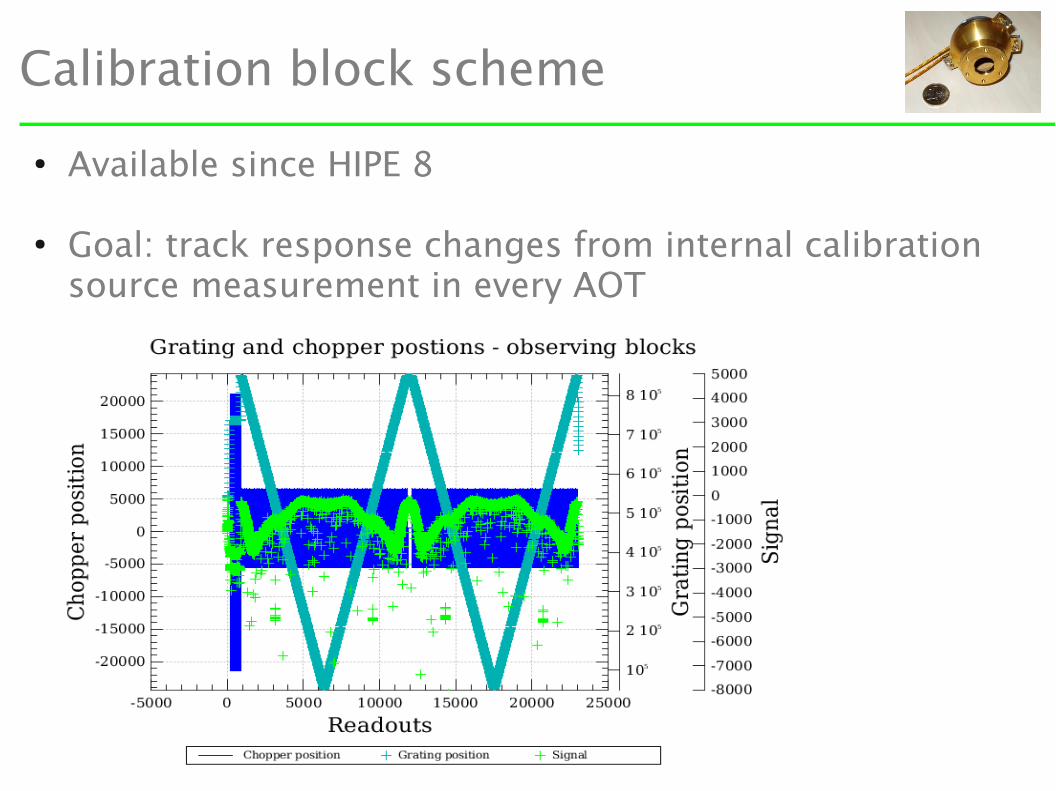
Calibration block scheme

● Available since HIPE 8

● Goal: track response changes from internal calibration source measurement in every AOT

Calibration block scheme (II)

● Calfile ObservedResponse: ● Average response central spaxel from sky fluxcal sources● Average response other pixels

– Flatfield from telescope background in chop OFF– Averaged over all abs. Flux cal obs– Scale flatfield to mean response central spaxel

● At key wavelength for each band● Calfile CalSourceFlux

● Average differential signal CS1-CS2 over all fluxcal obs● At key wavelength for each band

Telescope normalisation

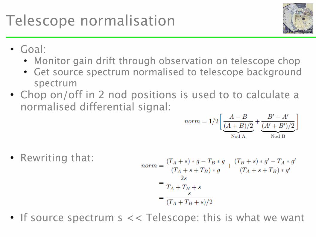
● Goal: ● Monitor gain drift through observation on telescope chop ● Get source spectrum normalised to telescope background

spectrum● Chop on/off in 2 nod positions is used to to calculate a

normalised differential signal:

● Rewriting that:

● If source spectrum s << Telescope: this is what we want

Telescope normalisation (II)

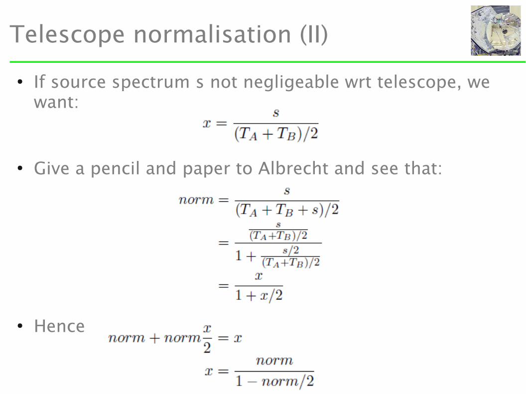
● If source spectrum s not negligeable wrt telescope, we want:

● Give a pencil and paper to Albrecht and see that:

● Hence

Telescope Normalisation (III)

● To get to source spectrum in Jansky, multiply normalisation pipeline result with telescope spectrum

● Calibration file TelescopeBackground● Based on Neptune raster observations / model ESA3

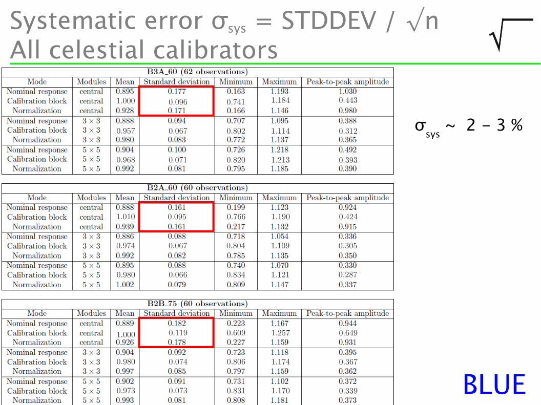
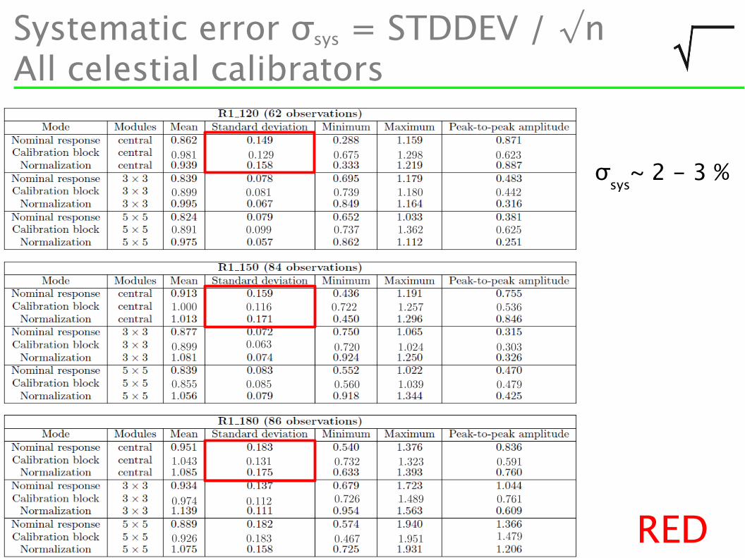
Systematic error σsys = STDDEV / √nAll celestial calibrators

σsys

~ 2 - 3 %

BLUE

1.010 0.095 0.766 1.190 0.424

0.974 0.067 0.804 1.109 0.305

0.2871.1210.8340.0660.980

1.000

0.957

0.968 0.071

0.067

0.096 0.741

0.802

0.820 1.213

1.114

1.184 0.443

0.312

0.393

1.000

0.980

0.973 0.073

0.074

0.119 0.609

0.806

0.831 1.170

1.174

1.257 0.649

0.367

0.339

Systematic error σsys = STDDEV / √nAll celestial calibrators

σsys

~ 2 - 3 %

RED

0.981 0.129 0.675 1.298 0.623

0.4421.1800.7390.0810.899

0.891 0.099 0.737 1.362 0.625

1.000

0.899

0.855

1.043

0.974

0.926

0.116

0.063

0.085

0.131

0.112

0.183

0.722 1.257 0.536

0.3031.0240.720

0.560 1.039 0.479

0.732

0.726

0.467 1.951

1.489

1.323 0.591

0.761

1.479

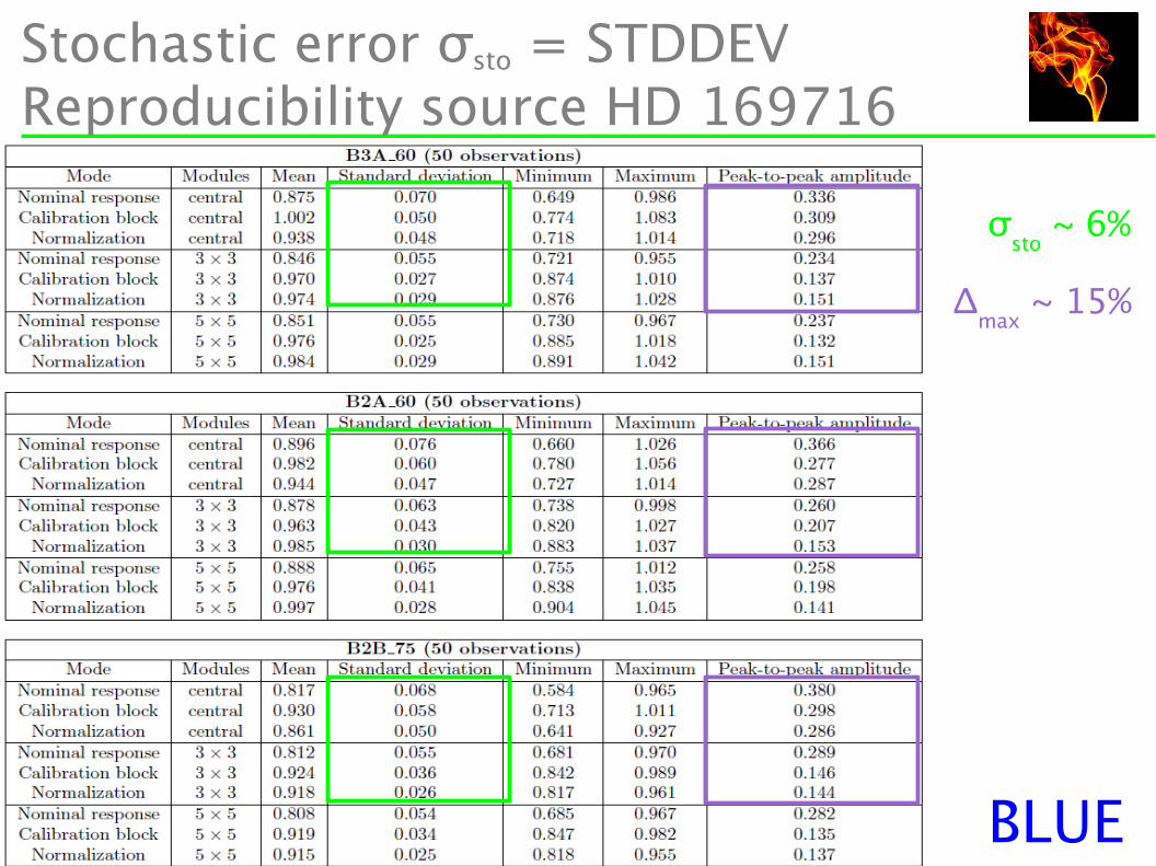
Stochastic error σsto = STDDEVReproducibility source HD 169716

σsto

~ 6%

Δmax

~ 15%

BLUE

Stochastic error σsto = STDDEVReproducibility source HD 169716

σsto

~ 5-7%

Δmax

~ 20%

RED

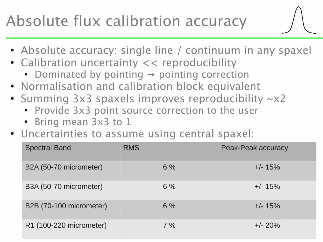
Absolute flux calibration accuracy

● Absolute accuracy: single line / continuum in any spaxel● Calibration uncertainty << reproducibility

● Dominated by pointing → pointing correction● Normalisation and calibration block equivalent● Summing 3x3 spaxels improves reproducibility ~x2

● Provide 3x3 point source correction to the user● Bring mean 3x3 to 1

● Uncertainties to assume using central spaxel:Spectral Band RMS Peak-Peak accuracy

B2A (50-70 micrometer) 6 % +/- 15%

B3A (50-70 micrometer) 6 % +/- 15%

B2B (70-100 micrometer) 6 % +/- 15%

R1 (100-220 micrometer) 7 % +/- 20%

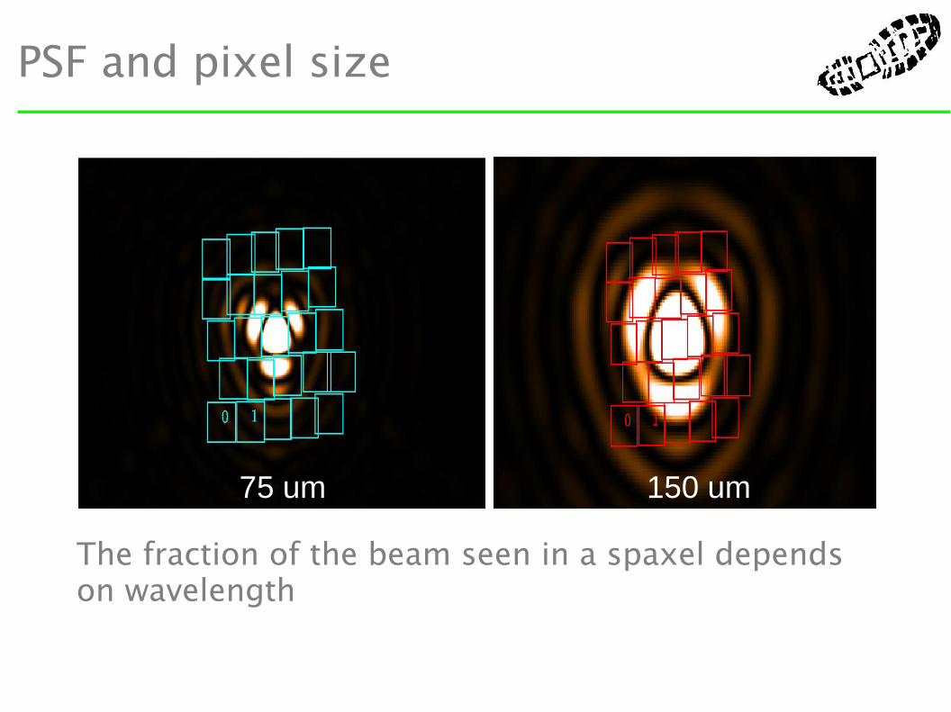
PSF and pixel size

The fraction of the beam seen in a spaxel depends on wavelength

75 um 150 um

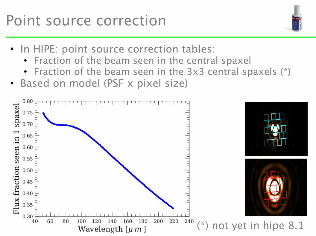
Point source correction

● In HIPE: point source correction tables:● Fraction of the beam seen in the central spaxel● Fraction of the beam seen in the 3x3 central spaxels (*)

● Based on model (PSF x pixel size)

(*) not yet in hipe 8.1

Point source correction verification

● All PACS SEDs:● Ratio central spaxel / 5x5 in final rebinned spectral cubes● Ratio central 3x3 / 5x5 in final rebinned spectral cubes● Median rebinned (filter out extended sources)

Point source correction

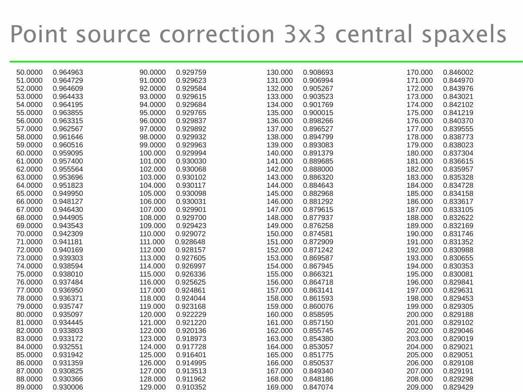
Point source correction 3x3 central spaxels 50.0000 0.964963 51.0000 0.964729 52.0000 0.964609 53.0000 0.964433 54.0000 0.964195 55.0000 0.963855 56.0000 0.963315 57.0000 0.962567 58.0000 0.961646 59.0000 0.960516 60.0000 0.959095 61.0000 0.957400 62.0000 0.955564 63.0000 0.953696 64.0000 0.951823 65.0000 0.949950 66.0000 0.948127 67.0000 0.946430 68.0000 0.944905 69.0000 0.943543 70.0000 0.942309 71.0000 0.941181 72.0000 0.940169 73.0000 0.939303 74.0000 0.938594 75.0000 0.938010 76.0000 0.937484 77.0000 0.936950 78.0000 0.936371 79.0000 0.935747 80.0000 0.935097 81.0000 0.934445 82.0000 0.933803 83.0000 0.933172 84.0000 0.932551 85.0000 0.931942 86.0000 0.931359 87.0000 0.930825 88.0000 0.930366 89.0000 0.930006

90.0000 0.929759 91.0000 0.929623 92.0000 0.929584 93.0000 0.929615 94.0000 0.929684 95.0000 0.929765 96.0000 0.929837 97.0000 0.929892 98.0000 0.929932 99.0000 0.929963 100.000 0.929994 101.000 0.930030 102.000 0.930068 103.000 0.930102 104.000 0.930117 105.000 0.930098 106.000 0.930031 107.000 0.929901 108.000 0.929700 109.000 0.929423 110.000 0.929072 111.000 0.928648 112.000 0.928157 113.000 0.927605 114.000 0.926997 115.000 0.926336 116.000 0.925625 117.000 0.924861 118.000 0.924044 119.000 0.923168 120.000 0.922229 121.000 0.921220 122.000 0.920136 123.000 0.918973 124.000 0.917728 125.000 0.916401 126.000 0.914995 127.000 0.913513 128.000 0.911962 129.000 0.910352

130.000 0.908693 131.000 0.906994 132.000 0.905267 133.000 0.903523 134.000 0.901769 135.000 0.900015 136.000 0.898266 137.000 0.896527 138.000 0.894799 139.000 0.893083 140.000 0.891379 141.000 0.889685 142.000 0.888000 143.000 0.886320 144.000 0.884643 145.000 0.882968 146.000 0.881292 147.000 0.879615 148.000 0.877937 149.000 0.876258 150.000 0.874581 151.000 0.872909 152.000 0.871242 153.000 0.869587 154.000 0.867945 155.000 0.866321 156.000 0.864718 157.000 0.863141 158.000 0.861593 159.000 0.860076 160.000 0.858595 161.000 0.857150 162.000 0.855745 163.000 0.854380 164.000 0.853057 165.000 0.851775 166.000 0.850537 167.000 0.849340 168.000 0.848186 169.000 0.847074

170.000 0.846002 171.000 0.844970 172.000 0.843976 173.000 0.843021 174.000 0.842102 175.000 0.841219 176.000 0.840370 177.000 0.839555 178.000 0.838773 179.000 0.838023 180.000 0.837304 181.000 0.836615 182.000 0.835957 183.000 0.835328 184.000 0.834728 185.000 0.834158 186.000 0.833617 187.000 0.833105 188.000 0.832622 189.000 0.832169 190.000 0.831746 191.000 0.831352 192.000 0.830988 193.000 0.830655 194.000 0.830353 195.000 0.830081 196.000 0.829841 197.000 0.829631 198.000 0.829453 199.000 0.829305 200.000 0.829188 201.000 0.829102 202.000 0.829046 203.000 0.829019 204.000 0.829021 205.000 0.829051 206.000 0.829108 207.000 0.829191 208.000 0.829298 209.000 0.829429

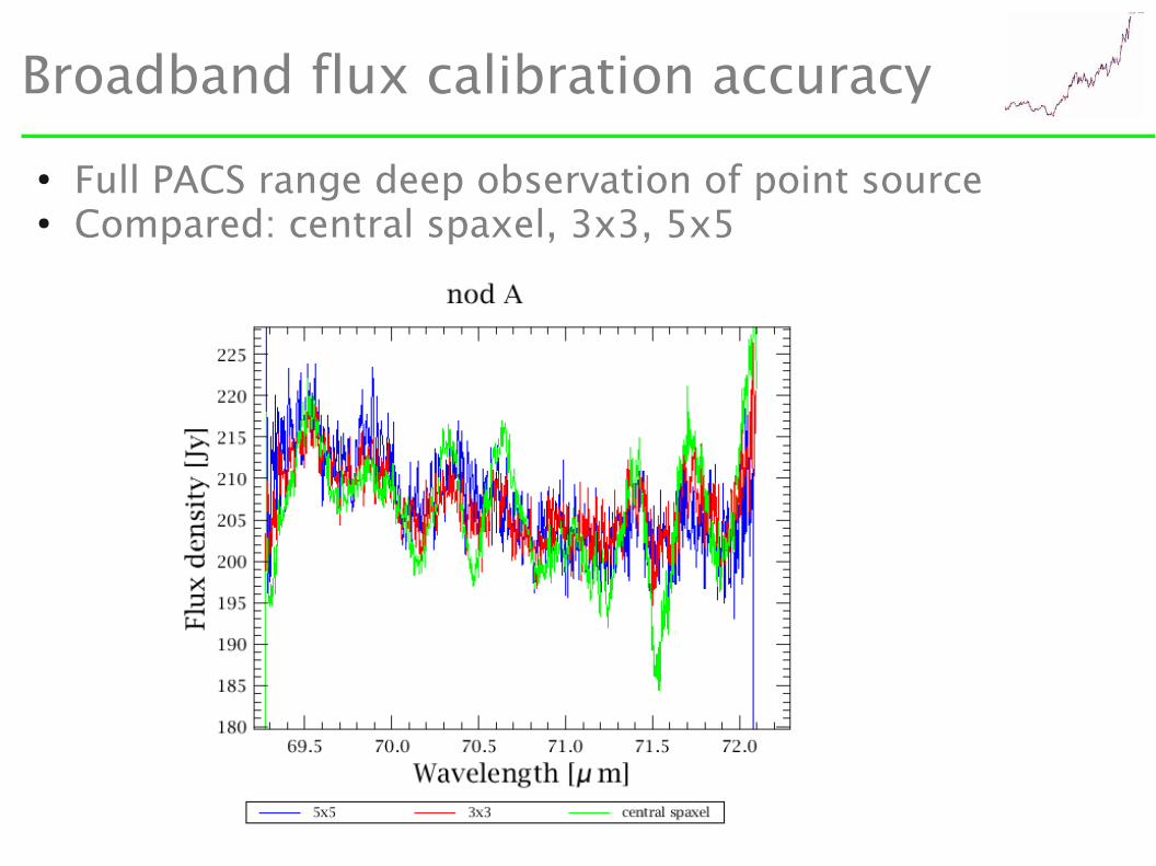
Broadband flux calibration accuracy

● Full PACS range deep observation of point source● Compared: central spaxel, 3x3, 5x5

Broadband flux calibration accuracy

● 3x3 sum best trade-off noise / continuum reliability● Pointing loss correction way forward

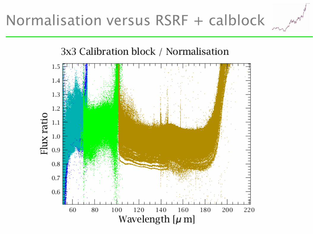
Normalisation versus RSRF + calblock

Broadband flux calibration accuracy

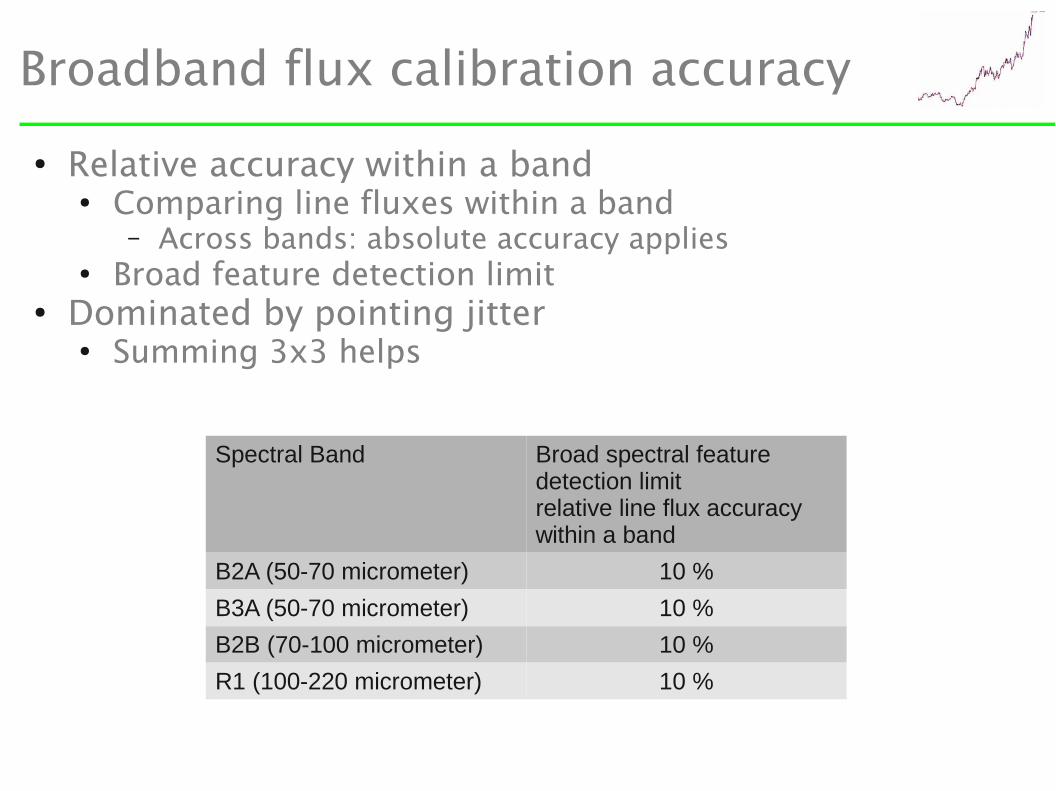
● Relative accuracy within a band● Comparing line fluxes within a band

– Across bands: absolute accuracy applies● Broad feature detection limit

● Dominated by pointing jitter● Summing 3x3 helps

Spectral Band Broad spectral feature detection limitrelative line flux accuracy within a band

B2A (50-70 micrometer) 10 %

B3A (50-70 micrometer) 10 %

B2B (70-100 micrometer) 10 %

R1 (100-220 micrometer) 10 %

Broadband accuracies - prospects

● Re-reduction RSRF measurements ILT● Band edge corrections● Comparison normalisation method: other slow

components● Pointing loss correction (pointing jitter)

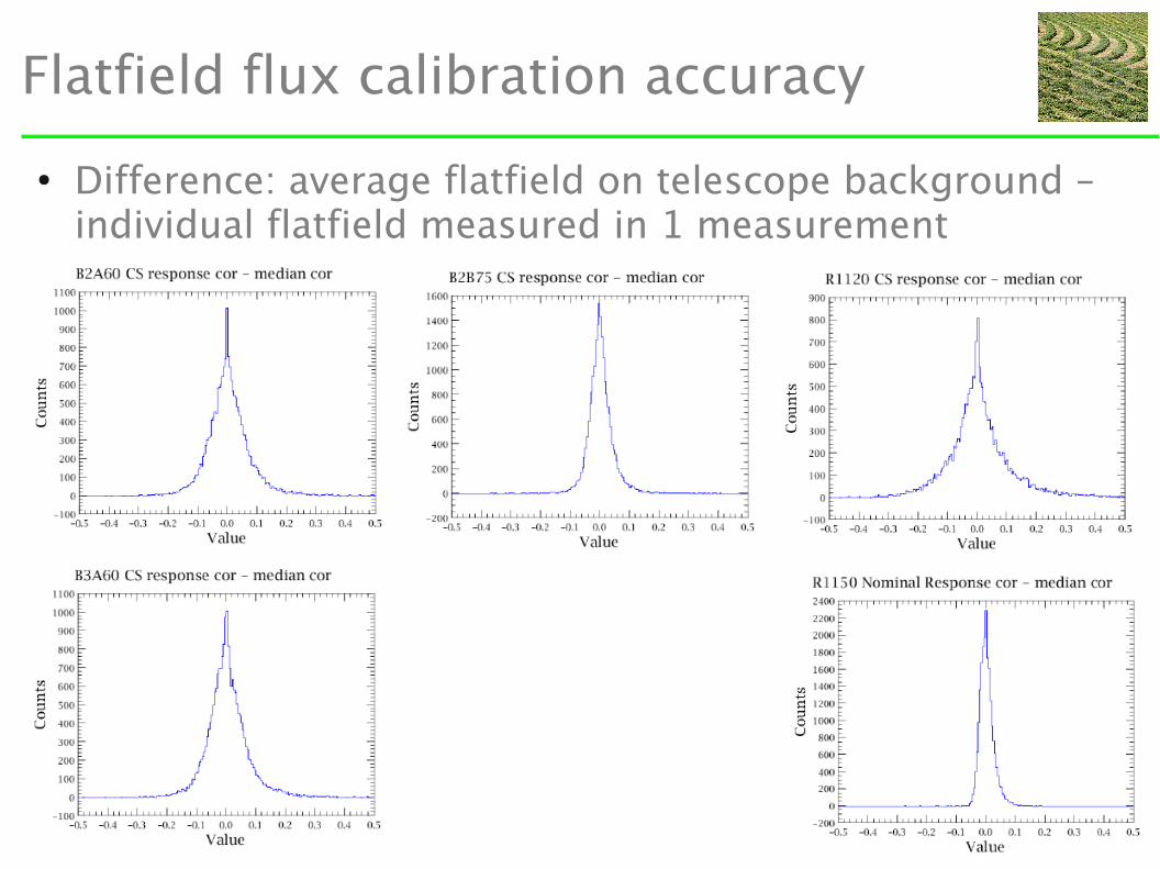
Flatfield flux calibration accuracy

● Difference: average flatfield on telescope background – individual flatfield measured in 1 measurement

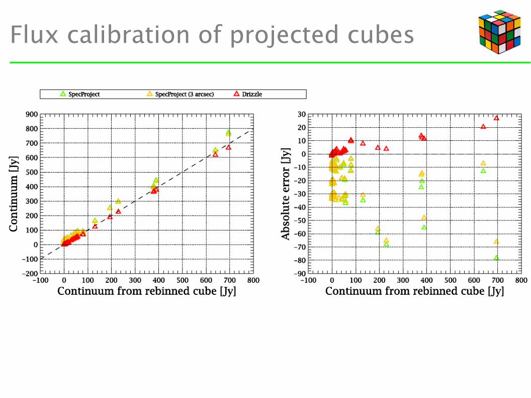
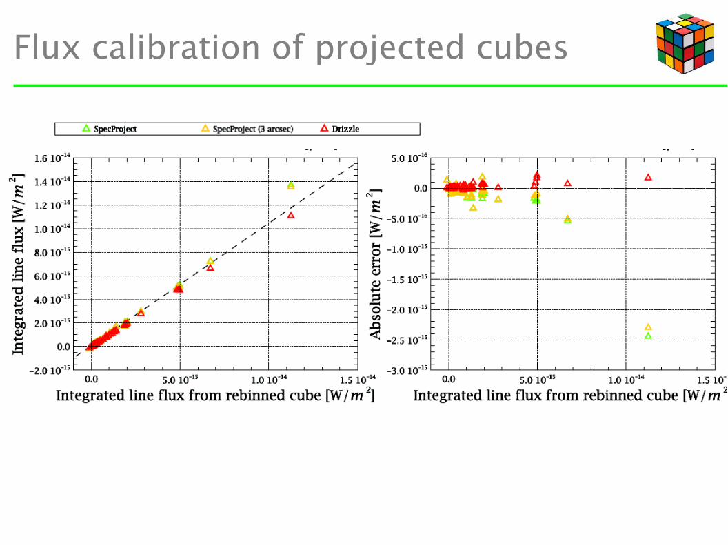
Flux calibration in projected cubes

● Comparison oversampled maps, line spectroscopy ● Rebinned spectrum

– central spaxel– central pointing in raster

● Projected cube– Co-added spectrum over central 9.4”x9.4”

● Cube projection:● Default 'specProject'

– naïve projection of rebinned spaxel spectra, 3” pixels● SpecProject, optimised pixel size

– Spatial pixel size optimised nyquist sampling beam● 3D drizzle

– Wavelength / spatial grid optimised for nyquist sampling– Shrinking pixels (avoid smearing)– Rebin in dot cloud

Flux calibration of projected cubes

Flux calibration of projected cubes

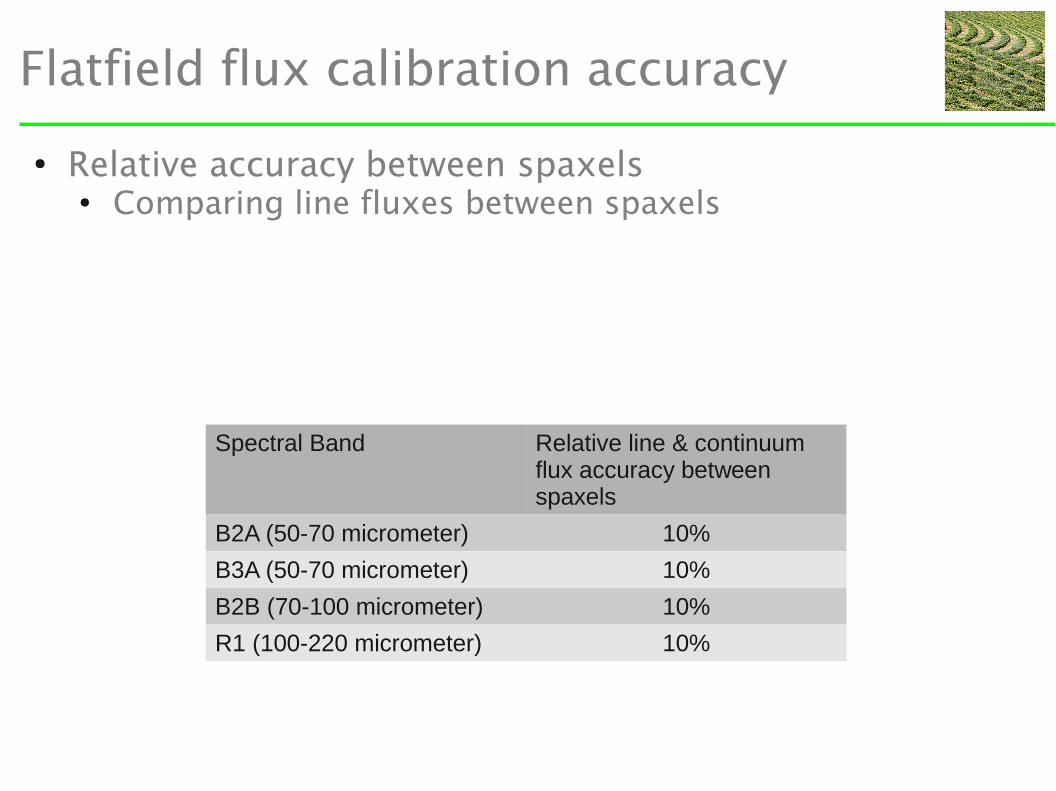
Flatfield flux calibration accuracy

● Relative accuracy between spaxels● Comparing line fluxes between spaxels

Spectral Band Relative line & continuum flux accuracy between spaxels

B2A (50-70 micrometer) 10%

B3A (50-70 micrometer) 10%

B2B (70-100 micrometer) 10%

R1 (100-220 micrometer) 10%

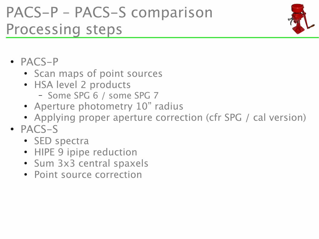
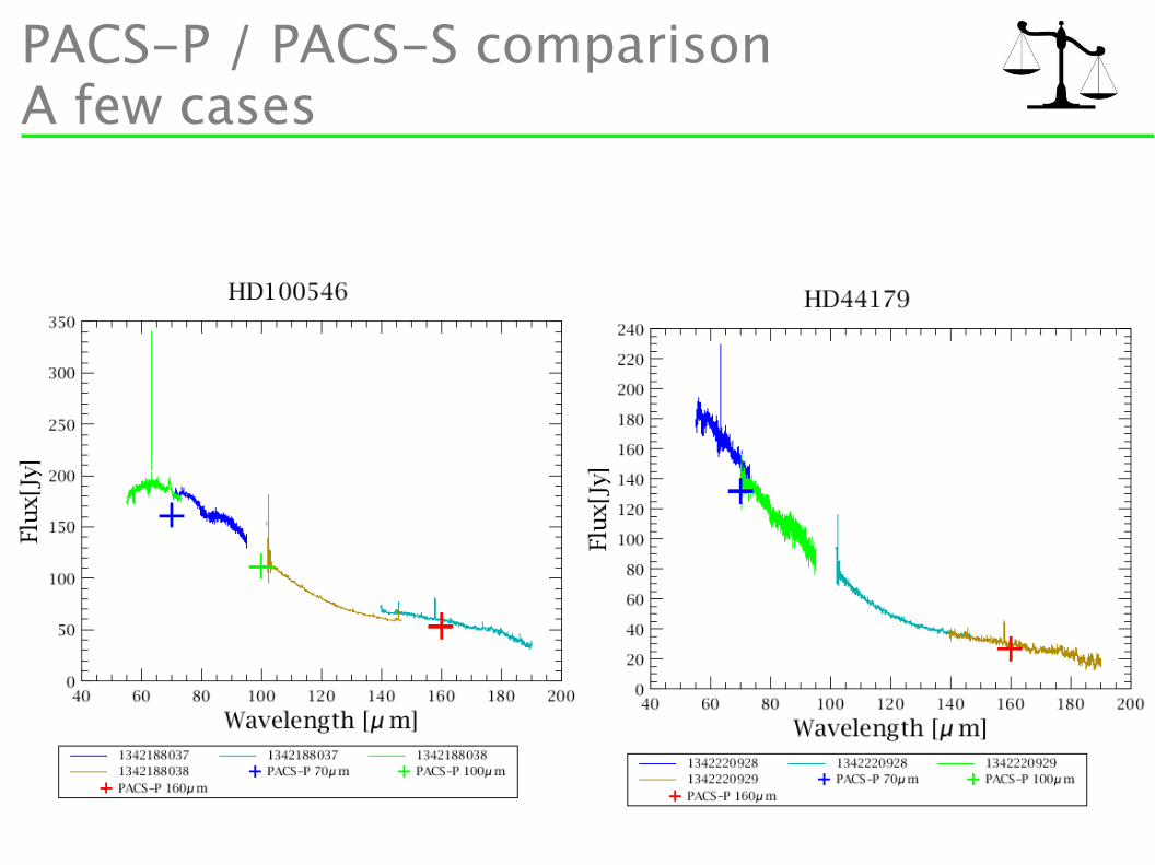
PACS-P – PACS-S comparisonProcessing steps

● PACS-P ● Scan maps of point sources ● HSA level 2 products

– Some SPG 6 / some SPG 7● Aperture photometry 10” radius● Applying proper aperture correction (cfr SPG / cal version)

● PACS-S● SED spectra● HIPE 9 ipipe reduction● Sum 3x3 central spaxels● Point source correction

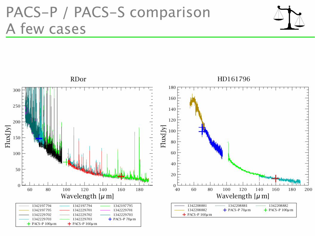
PACS-P / PACS-S comparisonA few cases

PACS-P / PACS-S comparisonA few cases

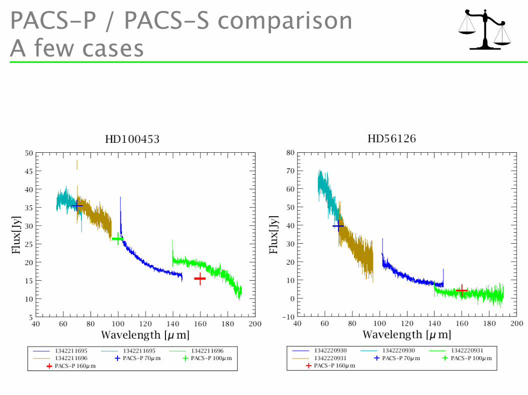
PACS-P / PACS-S comparisonA few cases

PACS-P / PACS-S comparisonConclusions & Outlook

● PACS-P – PACS-S agree within quoted error bars● On-going / planned:

● Reprocess PACS-P (proper high-pass, aperture centroid)● Extend with some more observations available

– PACS-P with inproper curve of growth were now rejected● Repeat comparison when spectrometer pointing correction

is available

Summary

● Wavelength calibration● Spectral leakage, 2nd pass ghosts● Absolute flux central spaxel 15%-20%, 3x3 7%-10%

● Compare central spaxel / 3x3 sums● Dominated by pointing

● Point source correction model appropriate ● Broadband accuracy 10%

● Band edge improvements● Leak regions● Dominated by pointing

● Spaxel-Spaxel calibration 10%● Consistency PACS-P and PACS-S within quoted errors

QUESTIONS ?