Pairwise Velocity Statistics in Convolution Lagrangian ...lilew/documents/BigBOSS... · 4 CLPT + RSD 5 Summary 6 Back up. Introduction CLPT: More resummation RSD: Gaussian streaming

Introduction CLPT: More resummation RSD: Gaussian streaming CLPT + RSD Summary Back up

Pairwise Velocity Statistics in ConvolutionLagrangian Perturbation Theory–Application to Redshift Space Distortions–

Lile Wang

Collaborator:Martin White (UC Berkeley/LBNL)

Beth A. Reid (LBNL, Hubble Fellow)

THCA/Dept. of Phys., Tsinghua UniversityLBNL

May 10, 2013


What’s Next?

1 IntroductionMotivations and BackgroundBefore resummationLagrangian resummation theory (LRT)

2 CLPT: More resummation

3 RSD: Gaussian streaming

4 CLPT + RSD

5 Summary

6 Back up


Motivations and Background

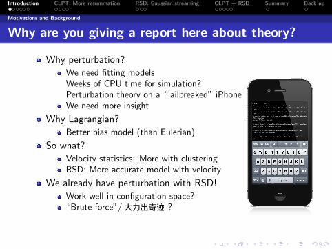
Why are you giving a report here about theory?

Why perturbation?

We need fitting modelsWeeks of CPU time for simulation?Perturbation theory on a “jailbreaked” iPhoneWe need more insight

Why Lagrangian?

Better bias model (than Eulerian)

So what?

Velocity statistics: More with clusteringRSD: More accurate model with velocity

We already have perturbation with RSD!

Work well in configuration space?“Brute-force”/ ?大力出奇迹


Before resummation

Lagrangian scheme: Basic introductions I

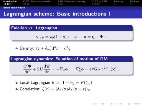
Eulerian vs. Lagrangian

v , ρ = ρ0(1 + δ) ; vs. x = q + Ψ .

Density: (1 + δm)d3x = d3q

Lagrangian dynamics: Equation of motion of DM

d2Ψ

dt2+ 2H

dΨ

dt= −∇xφ , ∇2

xφ = 4πGρ0a2δm(x) .

Local Lagrangian Bias: 1 + δX = F (δm)

Correlation: ξ(r) = 〈δX(x)δX(x + r)〉x


Before resummation

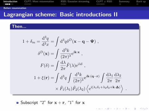
Lagrangian scheme: Basic introductions II

Then...

1 + δm =d3q

d3x=

∫d3qδD(x− q−Ψ) ,

δD(x) =

∫d3k

(2π)3eik·x ,

F (δ) =

∫dλ

2πF (λ)eiλδ ,

1 + ξ(r) =

∫d3q

∫d3k

(2π)3eik·(q−r)

∫dλ12π

dλ22π

× F1(λ1)F2(λ2)⟨

ei(λ1δ1+λ2δ2+k·∆)⟩.

Subscript “2” for x + r, “1” for x


Before resummation

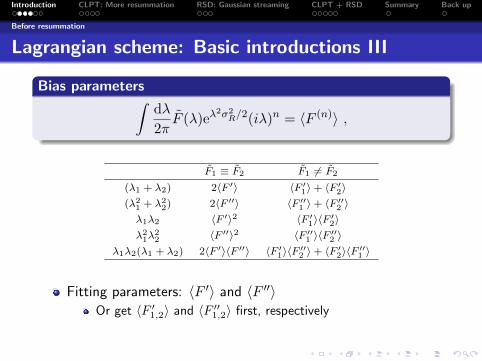
Lagrangian scheme: Basic introductions III

Bias parameters∫dλ

2πF (λ)eλ

2σ2R/2(iλ)n = 〈F (n)〉 ,

F1 ≡ F2 F1 6= F2

(λ1 + λ2) 2〈F ′〉〈F ′1〉+ 〈F ′2〉(λ21 + λ22) 2〈F ′′〉〈F ′′1 〉+ 〈F ′′2 〉λ1λ2 〈F ′〉2 〈F ′1〉〈F ′2〉λ21λ

22 〈F ′′〉2 〈F ′′1 〉〈F ′′2 〉

λ1λ2(λ1 + λ2) 2〈F ′〉〈F ′′〉〈F ′1〉〈F ′′2 〉+ 〈F ′2〉〈F ′′1 〉

Fitting parameters: 〈F ′〉 and 〈F ′′〉Or get 〈F ′1,2〉 and 〈F ′′1,2〉 first, respectively


Lagrangian resummation theory (LRT)

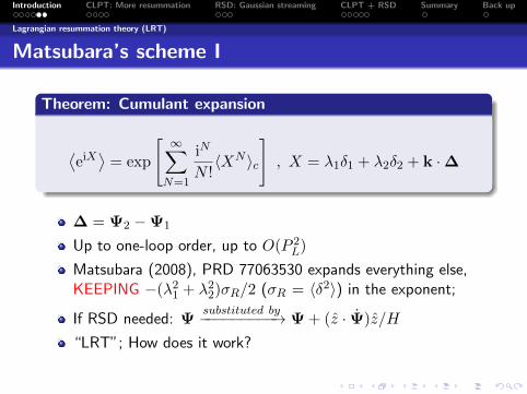
Matsubara’s scheme I

Theorem: Cumulant expansion

⟨eiX⟩

= exp

[ ∞∑N=1

iN

N !〈XN 〉c

], X = λ1δ1 + λ2δ2 + k ·∆

∆ = Ψ2 −Ψ1

Up to one-loop order, up to O(P 2L)

Matsubara (2008), PRD 77063530 expands everything else,KEEPING −(λ21 + λ22)σR/2 (σR = 〈δ2〉) in the exponent;

If RSD needed: Ψsubstituted by−−−−−−−−−→ Ψ + (z · Ψ)z/H

“LRT”; How does it work?


Lagrangian resummation theory (LRT)

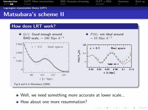
Matsubara’s scheme II

How does LRT work?

ξ(r): Good enough aroundBAO scale, ∼ 100 Mpc h−1

Fig 8 and 6 in Matsubara (2008)

P (k): not ideal around∼ 10 Mpc h−1

Well, we need something more accurate at lower scale...

How about one more resummation?


What’s Next?

1 Introduction

2 CLPT: More resummationCLPT: “Convolution” Lagrangian


4 CLPT + RSD

5 Summary

6 Back up


CLPT: “Convolution” Lagrangian

“Convolution”, or one more resummation

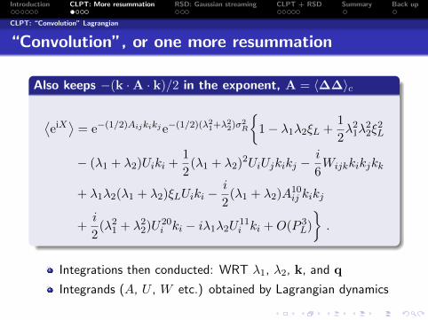
Also keeps −(k ·A · k)/2 in the exponent, A = 〈∆∆〉c

⟨eiX⟩

= e−(1/2)Aijkikje−(1/2)(λ21+λ

22)σ

2R

{1− λ1λ2ξL +

1

2λ21λ

22ξ

2L

− (λ1 + λ2)Uiki +1

2(λ1 + λ2)

2UiUjkikj −i

6Wijkkikjkk

+ λ1λ2(λ1 + λ2)ξLUiki −i

2(λ1 + λ2)A

10ij kikj

+i

2(λ21 + λ22)U

20i ki − iλ1λ2U11

i ki +O(P 3L)

}.

Integrations then conducted: WRT λ1, λ2, k, and q

Integrands (A, U , W etc.) obtained by Lagrangian dynamics



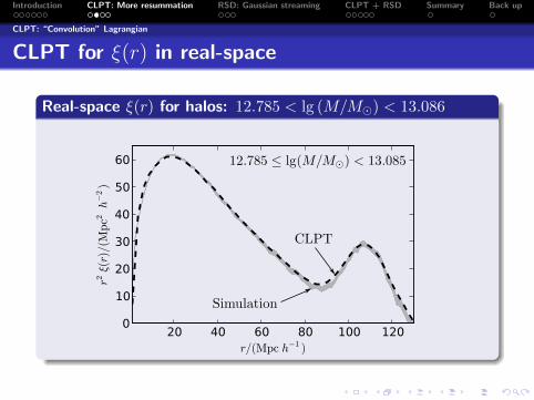
CLPT for ξ(r) in real-space

Real-space ξ(r) for halos: 12.785 < lg (M/M�) < 13.086



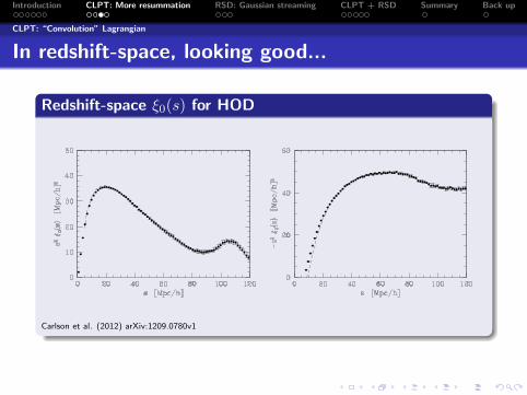
In redshift-space, looking good...

Redshift-space ξ0(s) for HOD

Carlson et al. (2012) arXiv:1209.0780v1



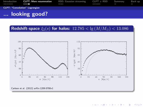
... looking good?

Redshift-space ξ2(s) for halos: 12.785 < lg (M/M�) < 13.086

Carlson et al. (2012) arXiv:1209.0780v1


What’s Next?

1 Introduction


3 RSD: Gaussian streamingLinear and quasi-linear RSD

4 CLPT + RSD

5 Summary

6 Back up


Linear and quasi-linear RSD

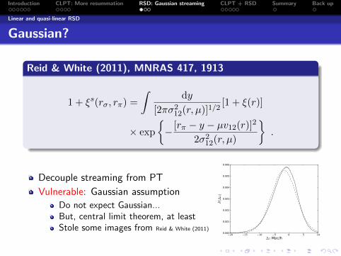
Gaussian?

Reid & White (2011), MNRAS 417, 1913

1 + ξs(rσ, rπ) =

∫dy

[2πσ212(r, µ)]1/2[1 + ξ(r)]

× exp

{− [rπ − y − µv12(r)]2

2σ212(r, µ)

}.

Decouple streaming from PT

Vulnerable: Gaussian assumption

Do not expect Gaussian...But, central limit theorem, at leastStole some images from Reid & White (2011)



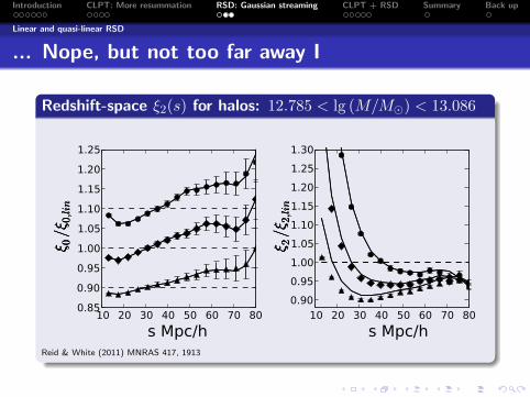
... Nope, but not too far away I


Reid & White (2011) MNRAS 417, 1913



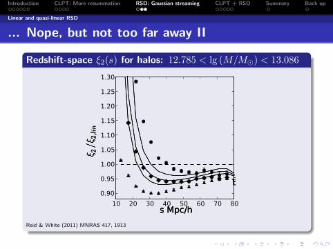
... Nope, but not too far away II


Reid & White (2011) MNRAS 417, 1913


What’s Next?

1 Introduction



4 CLPT + RSDVelocity statistics

5 Summary

6 Back up


Velocity statistics

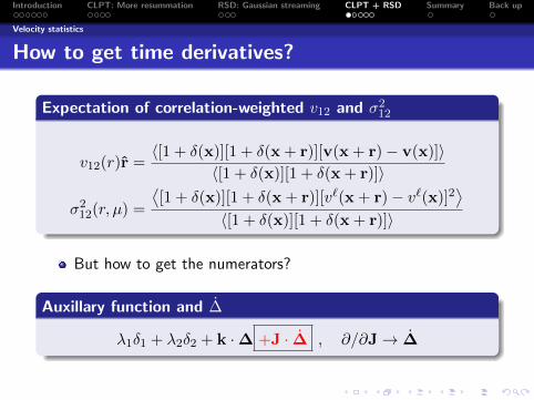
How to get time derivatives?

Expectation of correlation-weighted v12 and σ212

v12(r)r =〈[1 + δ(x)][1 + δ(x + r)][v(x + r)− v(x)]〉

〈[1 + δ(x)][1 + δ(x + r)]〉

σ212(r, µ) =

⟨[1 + δ(x)][1 + δ(x + r)][v`(x + r)− v`(x)]2

⟩〈[1 + δ(x)][1 + δ(x + r)]〉

But how to get the numerators?

Auxillary function and ∆

λ1δ1 + λ2δ2 + k ·∆ +J · ∆ , ∂/∂J→ ∆


Velocity statistics

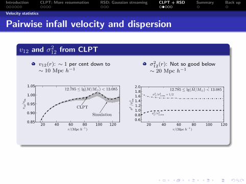
Pairwise infall velocity and dispersion

v12 and σ212 from CLPT

v12(r): ∼ 1 per cent down to∼ 10 Mpc h−1

σ212(r): Not so good below

∼ 20 Mpc h−1


Velocity statistics

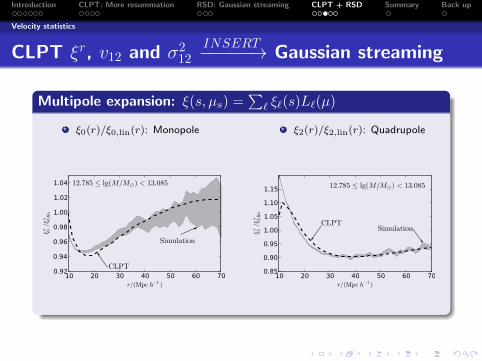
CLPT ξr, v12 and σ212

INSERT−−−−−→ Gaussian streaming

Multipole expansion: ξ(s, µs) =∑

` ξ`(s)L`(µ)

ξ0(r)/ξ0,lin(r): Monopole ξ2(r)/ξ2,lin(r): Quadrupole


Velocity statistics

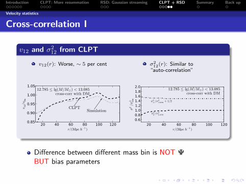
Cross-correlation I

v12 and σ212 from CLPT

v12(r): Worse, ∼ 5 per cent σ212(r): Similar to

“auto-correlation”

Difference between different mass bin is NOT ΨBUT bias parameters


Velocity statistics

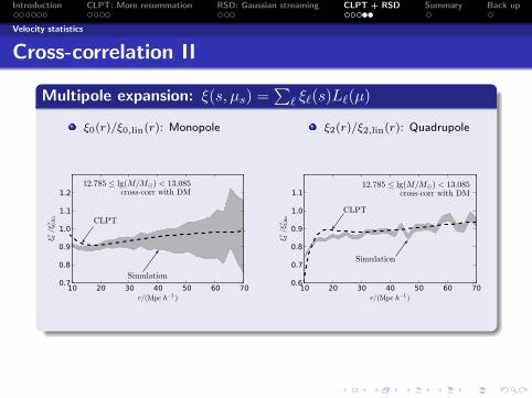
Cross-correlation II

Multipole expansion: ξ(s, µs) =∑

` ξ`(s)L`(µ)

ξ0(r)/ξ0,lin(r): Monopole ξ2(r)/ξ2,lin(r): Quadrupole


What’s Next?

1 Introduction



4 CLPT + RSD

5 SummarySummary and Conclusions

6 Back up


Summary and Conclusions

Summary

One more resummation: Improvement, only 2(3) parameters

Real-space ξr improvedReal-space v12 improved (σ2

12 a little bit worse)

Scale-independent local Lagrangian bias: Halos applicable (?)

Gaussian streaming gives good output for good input (CLPT)

∼ 1 per cent at <∼ 15 Mpc h−1

∼ 10 per cent at <∼ 10 Mpc h−1

Works well for monopole and quadrupole

Possible applications:

RS correlation → Cosmology + Bias parameters → v12, σ2

Perturbations are still fast enough on an iPhone

Documents

Pairwise Velocity Statistics in Convolution Lagrangian ...lilew/documents/BigBOSS... · 4 CLPT + RSD 5 Summary 6 Back up. Introduction CLPT: More resummation RSD: Gaussian streaming