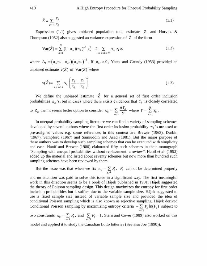
© 2016 Pakistan Journal of Statistics 409

Pak. J. Statist.

2016 Vol. 32(6), 409-423

A HIGH ENTROPY PROCEDURE FOR UNEQUAL PROBABILITY SAMPLING

Aftab Ahmad and Muhammad Hanif

National College of Business Administration and Economics, Lahore, Pakistan

Email: aftab.stat@gmail.com, drmainhanif@gmail.com

ABSTRACT

In survey sampling we select a random sample according to some specified random

fashion. We focused to apply innovative approach of maximum entropy sampling to

develop a new easily executable procedure to determine the probability function in

unequal probability sampling and it needs no iteration to compute inclusion probabilities

of any order. The empirical comparison of this procedure shows that Horvitz &

Thompson (1952) population total estimate has high entropy and lower variance than that

of the Yates and Grundy (1953), Brewer (1963) and Prabhu and Ajgankar (1982)

selection procedures.

KEY WORDS

Probability proportional to size sampling, Entropy, Horvitz & Thompson Population

estimate, First & second (or joint) order probabilities of inclusion.

1. INTRODUCTION

In unequal probability sampling without replacement consider a finite population

comprising of N elements or units. For each such element k , where 1,2,3, ,k N ,

two variables Y and Z are attached such that the values of the variable Y , called as

benchmark or auxiliary variable, is known for all the values of k from 1 to N . The

variable of main interest is denoted by Z and we want to estimate the population total

1

N

kk

Z Z

. The benchmark or auxiliary variable Y is supposed to be related to the

variable of interest Z . We select n distinct units as a random sample from the finite

population and for those selected units k in the sample the values of the main variable

kZ are then known. The probability to select a sample s is represented by sP . Since

sampling is without replacement so there being altogether NnC distinct samples and

1ss

P

, where Ω denotes the collection of all possible samples. The first order

inclusion probability or probability of inclusion of unit k in the sample is denoted by k

where k ss k

P

. For k the property 1

N

kk

n

, holds. With such k ’s a popular

estimator of population total Z , suggested by the Horvitz & Thompson (1952) is

A High Entropy Procedure for Unequal Probability Sampling 410

ˆ k

k s k

zZ

(1.1)

Expression (1.1) gives unbiased population total estimate Z and Horvitz &

Thompson (1952) also suggested an variance expression of Z of the form

1 2

1 1

ˆVar( ) (1 )( ) 2N

k k k k k lk k l N

Z z z z

(1.2)

where 1

k k l kl k l

. If 0kl , Yates and Grundy (1953) provided an

unbiased estimate ˆ( )v Z of ˆVar( )Z where

2

ˆ( ) k lk

k l s k l

z zv Z

(1.3)

We define the unbiased estimate Z for a general set of first order inclusion

probabilities k ’s, but in cases where there exists evidences that kY is closely correlated

to kZ then it seems better option to consider kk

k s

nY

Y

where 1

N

kk

Y Y

.

In unequal probability sampling literature we can find a variety of sampling schemes

developed by several authors where the first order inclusion probability k ’s are used as

pre-assigned values e.g. some references in this context are Brewer (1963), Durbin

(1967), Sampford (1967) and Samiuddin and Asad (1981). But the major purpose of

these authors was to develop such sampling schemes that can be executed with simplicity

and ease. Hanif and Brewer (1980) elaborated fifty such schemes in their monograph

“Sampling with unequal probabilities without replacement: a review”. Hanif et al. (1992)

added up the material and listed about seventy schemes but now more than hundred such

sampling schemes have been reviewed by them.

But the issue was that when we fix ,k ss k

P

sP cannot be determined properly

and no attention was paid to solve this issue in a significant way. The first meaningful

work in this direction seems to be a book of Hájek published in 1981. Hájek suggested

the theory of Poisson sampling design. This design maximizes the entropy for first order

inclusion probabilities but it suffers due to the variable sample size. Hájek suggested to

use a fixed sample size instead of variable sample size and provided the idea of

conditional Poisson sampling which is also known as rejective sampling. Hájek derived

Conditional Poisson sampling by maximizing entropy criteria ln( )s ss

P P

subject to

two constraints ,k ss k

P

and 1ss

P

. Stern and Cover (1989) also worked on this

model and applied it to study the Canadian Lotto lotteries (See also Joe (1990)).

Ahmad and Hanif 411

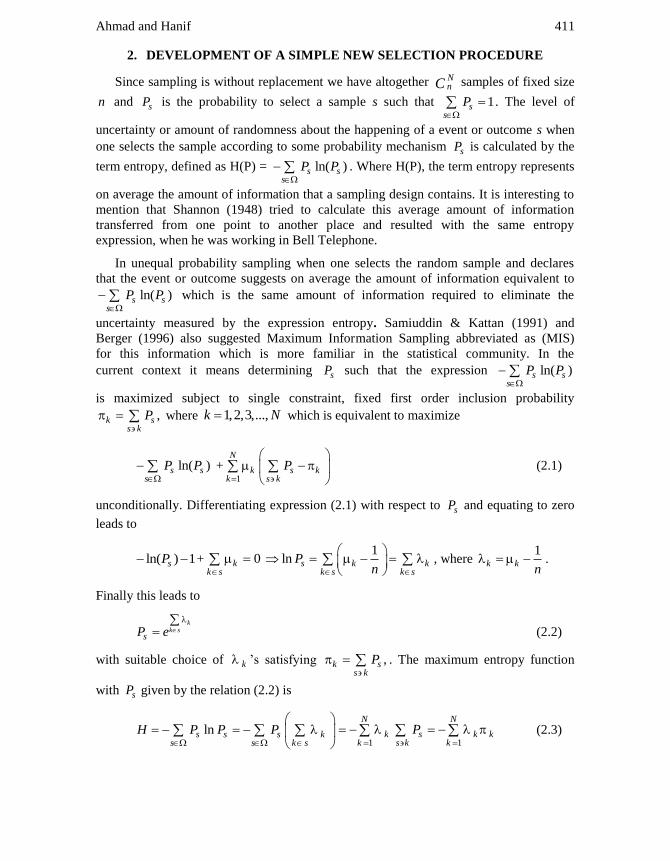
2. DEVELOPMENT OF A SIMPLE NEW SELECTION PROCEDURE

Since sampling is without replacement we have altogether NnC samples of fixed size

n and sP is the probability to select a sample s such that 1ss

P

. The level of

uncertainty or amount of randomness about the happening of a event or outcome s when

one selects the sample according to some probability mechanism sP is calculated by the

term entropy, defined as H(P) = ln( )s ss

P P

. Where H(P), the term entropy represents

on average the amount of information that a sampling design contains. It is interesting to

mention that Shannon (1948) tried to calculate this average amount of information

transferred from one point to another place and resulted with the same entropy

expression, when he was working in Bell Telephone.

In unequal probability sampling when one selects the random sample and declares

that the event or outcome suggests on average the amount of information equivalent to

ln( )s ss

P P

which is the same amount of information required to eliminate the

uncertainty measured by the expression entropy. Samiuddin & Kattan (1991) and

Berger (1996) also suggested Maximum Information Sampling abbreviated as (MIS)

for this information which is more familiar in the statistical community. In the

current context it means determining sP such that the expression ln( )s ss

P P

is maximized subject to single constraint, fixed first order inclusion probability

,k ss k

P

where 1,2,3,...,k N which is equivalent to maximize

ln( )s ss

P P

+1

N

k s kk s k

P

(2.1)

unconditionally. Differentiating expression (2.1) with respect to sP and equating to zero

leads to

ln( ) 1sP + 0kk s

1

ln s k kk s k s

Pn

, where

1k k

n .

Finally this leads to

k

k ssP e

(2.2)

with suitable choice of k ’s satisfying ,k ss k

P

. The maximum entropy function

with sP given by the relation (2.2) is

lns s s ks s k s

H P P P

1 1

N N

k s k kk s k k

P

(2.3)

A High Entropy Procedure for Unequal Probability Sampling 412

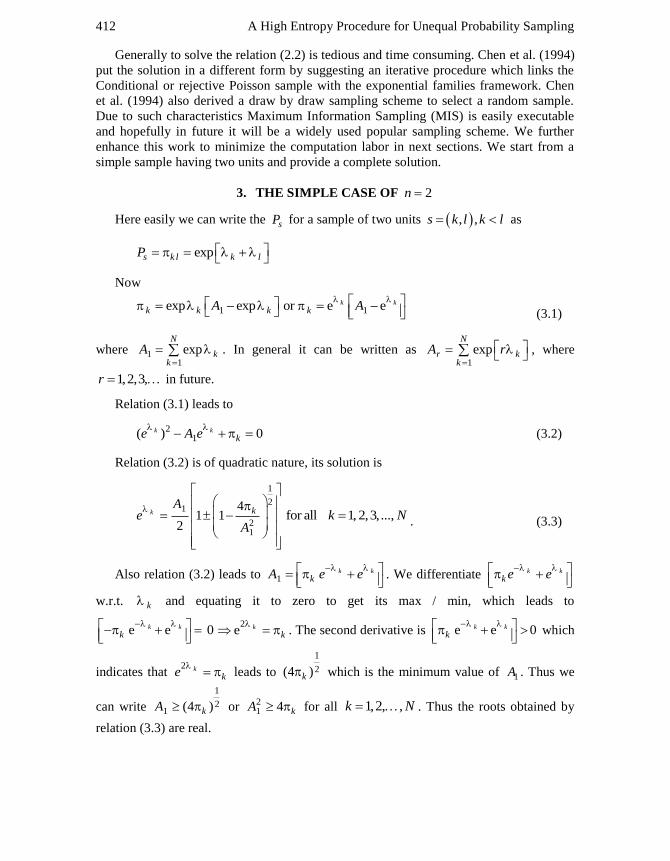
Generally to solve the relation (2.2) is tedious and time consuming. Chen et al. (1994)

put the solution in a different form by suggesting an iterative procedure which links the

Conditional or rejective Poisson sample with the exponential families framework. Chen

et al. (1994) also derived a draw by draw sampling scheme to select a random sample.

Due to such characteristics Maximum Information Sampling (MIS) is easily executable

and hopefully in future it will be a widely used popular sampling scheme. We further

enhance this work to minimize the computation labor in next sections. We start from a

simple sample having two units and provide a complete solution.

3. THE SIMPLE CASE OF 2n

Here easily we can write the sP for a sample of two units , ,s k l k l as

exps k l k lP

Now

1 1exp exp or e ek k

k k k kA A (3.1)

where 11

expN

kk

A

. In general it can be written as 1

expN

r kk

A r

, where

1,2,3,r in future.

Relation (3.1) leads to

2

1( ) 0k k

ke A e

(3.2)

Relation (3.2) is of quadratic nature, its solution is

1

21

21

41 1

2

k kA

eA

for all 1, 2,3,...,k N. (3.3)

Also relation (3.2) leads to 1k k

kA e e

. We differentiate k k

k e e

w.r.t. k and equating it to zero to get its max / min, which leads to

e e 0k k

k

2e k

k

. The second derivative is e e 0k k

k

which

indicates that 2 k

ke

leads to

1

2(4 )k which is the minimum value of 1A . Thus we

can write

1

21 (4 )kA or

21 4 kA for all 1,2, ,k N . Thus the roots obtained by

relation (3.3) are real.

Ahmad and Hanif 413

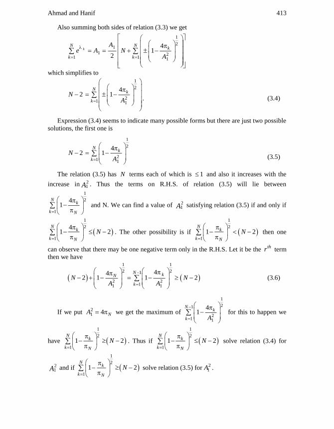
Also summing both sides of relation (3.3) we get

1

21

1 21 1 1

41

2

kN N

k

k k

Ae A N

A

which simplifies to

1

2

21 1

42 1

Nk

k

NA

. (3.4)

Expression (3.4) seems to indicate many possible forms but there are just two possible

solutions, the first one is

1

2

21 1

42 1

Nk

k

NA

(3.5)

The relation (3.5) has N terms each of which is 1 and also it increases with the

increase in 21A . Thus the terms on R.H.S. of relation (3.5) will lie between

1

2

1

41

Nk

k N

and N. We can find a value of 21A satisfying relation (3.5) if and only if

1

2

1

41 2

Nk

k N

N

. The other possibility is if

1

2

1

1 2N

k

k N

N

then one

can observe that there may be one negative term only in the R.H.S. Let it be the thr term

then we have

1 1

2 21

2 211 1

442 1 1 2

N kN

k

N NA A

(3.6)

If we put 21 4 NA we get the maximum of

1

21

21 1

41

Nk

k A

for this to happen we

have

1

2

1

1 2N

k

k N

N

. Thus if

1

2

1

1 2N

k

k N

N

solve relation (3.4) for

21A and if

1

2

1

1 2N

k

k N

N

solve relation (3.5) for21A .

A High Entropy Procedure for Unequal Probability Sampling 414

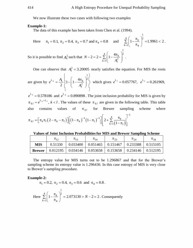
We now illustrate these two cases with following two examples

Example-1:

The data of this example has been taken from Chen et al. (1994).

Here 1 2 3 40.1, 0.4, 0.7 and 0.8 and

1

4 2

1 4

1 1.9961 2k

k

.

So it is possible to find 21A such that

1

24

21 1

42 2 1 k

k

NA

.

One can observe that 21 3.20005A nearly satisfies the equation. For MIS the roots

are given by

1

21

21

41 1

2

k kAe

A

which gives 1 0.057767,e 2 0.261969,e

3 0.578186e

and 4 0.890898e

. The joint inclusion probability for MIS is given by

,k l

k l e k l

. The values of these k l are given in the following table. This table

also contains values of k l for Brewer sampling scheme where

141 1

1

2 1 1 21

kk l k l k l k l

k l

Values of Joint Inclusion Probabilities for MIS and Brewer Sampling Scheme

12 13

14 23

24 34

MIS 0.51330 0.033400 0.051465 0.151467 0.233388 0.515105

Brewer 0.012195 0.034146 0.053658 0.153658 0.234146 0.512195

The entropy value for MIS turns out to be 1.296867 and that for the Brewer’s

sampling scheme its entropy value is 1.296436. In this case entropy of MIS is very close

to Brewer’s sampling procedure.

Example-2:

1 2 3 40.2, 0.4, 0.6 and 0.8 .

Here

1

4 2

1 4

1 2.073130 2 2k

k

N

. Consequently

Ahmad and Hanif 415

1 1

2 234

2 21 1 1

4 42 2 1 1k

k

NA A

(3.7)

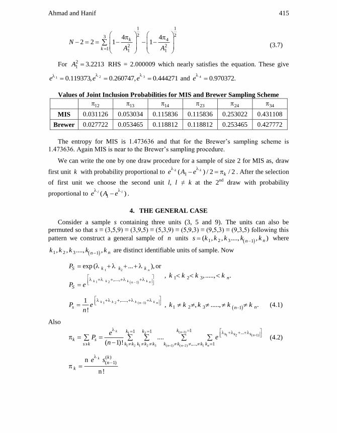
For 21 3.2213A RHS = 2.000009 which nearly satisfies the equation. These give

2 31 0.119373, 0.260747, 0.444271e e e

and 4 0.970372.e

Values of Joint Inclusion Probabilities for MIS and Brewer Sampling Scheme

12 13

14 23

24 34

MIS 0.031126 0.053034 0.115836 0.115836 0.253022 0.431108

Brewer 0.027722 0.053465 0.118812 0.118812 0.253465 0.427772

The entropy for MIS is 1.473636 and that for the Brewer’s sampling scheme is

1.473636. Again MIS is near to the Brewer’s sampling procedure.

We can write the one by one draw procedure for a sample of size 2 for MIS as, draw

first unit k with probability proportional to 1( ) / 2 / 2k k

ke A e

. After the selection

of first unit we choose the second unit l, l ≠ k at the 2nd

draw with probability

proportional to 1( )l le A e

.

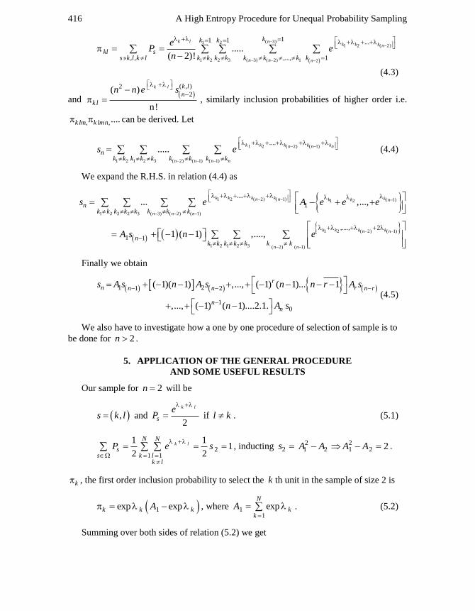
4. THE GENERAL CASE

Consider a sample s containing three units (3, 5 and 9). The units can also be

permuted so that s ≡ (3,5,9) ≡ (3,9,5) ≡ (5,3,9) ≡ (5,9,3) ≡ (9,5,3) ≡ (9,3,5) following this

pattern we construct a general sample of n units 1 2 3 1( , , ...., , )nn

s k k k k k

where

1 2 3 1, , ...., , nn

k k k k k

are distinct identifiable units of sample. Now

1 2

1 2 1,....,

exp ( ... ), orn

k k k k nn

S k k k

S

P

P e

, 1 2 3, ....., .nk k k k

1 2 ( 1),.....,1

!

k k k kn n

sP en

, 1 2 3 1

, ....., .nnk k k k k

(4.1)

Also

( 1)1 2

1 2 ( 1)

1 2 1 2 3 ( 1) ( 2) 1

11 1 ...

,..., 1

....( 1)!

k nk k k n

n n n

kk k

k ss k k k k k k k k k k

eP e

n

(4.2)

( )( 1)n

n!

k kn

k

e s

A High Entropy Procedure for Unequal Probability Sampling 416

( 3)1 21 2 ( 2)

1 2 2 3 ( 3) ( 2) 1 2

11 1 ...

, , ,..., 1

.....( 2)!

k l nk k k n

n n n

kk k

kl ss k l k l k k k k k k k k

eP e

n

(4.3)

and ( , )2

2( )

n!

k l k l

n

k l

n n e s

, similarly inclusion probabilities of higher order i.e.

, ,....k lm k lmn can be derived. Let

1 2 ( 2) ( 1)

1 2 1 2 3 ( 2) ( 1) ( 1)

.........

k k k k kn n n

n n n n

nk k k k k k k k k

s e

(4.4)

We expand the R.H.S. in relation (4.4) as

1 2 ( 2) ( 1)

1 2 2 2 3 ( 3) ( 2) ( 1)

.......

k k k kn n

n n n

nk k k k k k k k

s e

( 1)1 21 ,...,

kk k nA e e e

1 1nA s

1 2 ( 2) ( 1)

1 2 1 2 3 ( 2) ( 1)

,...., 21 ( 1) ,....,

k k k kn n

n nk k k k k k k

n e

Finally we obtain

1 21 2

10

( 1)( 1) ,..., ( 1) ( 1)... 1

,..., ( 1) ( 1)....2.1.

rn rn n n r

nn

s A s n A s n n r A s

n A s

(4.5)

We also have to investigate how a one by one procedure of selection of sample is to

be done for 2n .

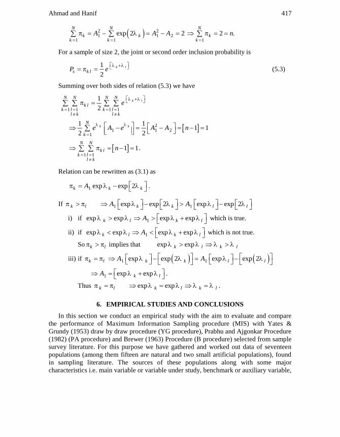
5. APPLICATION OF THE GENERAL PROCEDURE

AND SOME USEFUL RESULTS

Our sample for 2n will be

,s k l and 2

k l

s

eP

if l k . (5.1)

21 1

1 11

2 2

k lN N

ss k l

k l

P e s

, inducting 22 1 2s A A 2

1 2 2A A .

k , the first order inclusion probability to select the k th unit in the sample of size 2 is

1exp expk k kA , where 11

expN

kk

A

. (5.2)

Summing over both sides of relation (5.2) we get

Ahmad and Hanif 417

2 21 1 2

1 1

exp 2 2N N

k kk k

A A A

1

2 .N

kk

n

For a sample of size 2, the joint or second order inclusion probability is

1

2

k l

s k lP e (5.3)

Summing over both sides of relation (5.3) we have

1 1 1 1

1

2

k lN N N N

k lk l k l

l k l k

e

21 1 2

1

1 11 1

2 2

k kN

k

e A e A A n

1 1

1 1N N

k lk l

l k

n

.

Relation can be rewritten as (3.1) as

1 exp exp 2k k kA .

If 1 1exp exp 2 exp exp 2k l k k l lA A

i) if 1exp exp exp expk l k lA which is true.

ii) if 1exp exp exp expk l k lA which is not true.

So k l implies that exp expk l k l

iii) if 1 1exp exp 2 exp exp 2k l k k l lA A

1 exp expk lA .

Thus exp expk l k l k l .

6. EMPIRICAL STUDIES AND CONCLUSIONS

In this section we conduct an empirical study with the aim to evaluate and compare

the performance of Maximum Information Sampling procedure (MIS) with Yates &

Grundy (1953) draw by draw procedure (YG procedure), Prabhu and Ajgonkar Procedure

(1982) (PA procedure) and Brewer (1963) Procedure (B procedure) selected from sample

survey literature. For this purpose we have gathered and worked out data of seventeen

populations (among them fifteen are natural and two small artificial populations), found

in sampling literature. The sources of these populations along with some major

characteristics i.e. main variable or variable under study, benchmark or auxiliary variable,

A High Entropy Procedure for Unequal Probability Sampling 418

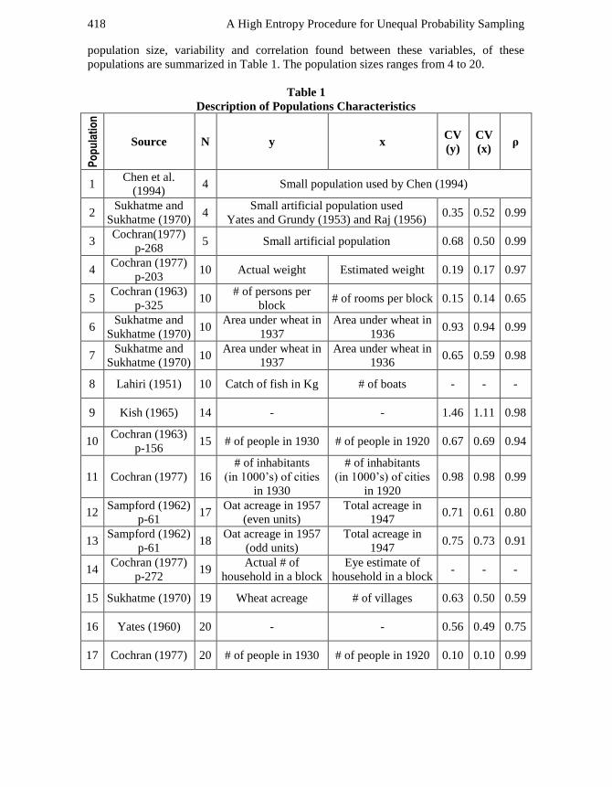
population size, variability and correlation found between these variables, of these

populations are summarized in Table 1. The population sizes ranges from 4 to 20.

Table 1

Description of Populations Characteristics

Po

pu

lati

on

Source N y x CV

(y)

CV

(x) ρ

1 Chen et al.

(1994) 4 Small population used by Chen (1994)

2 Sukhatme and

Sukhatme (1970) 4

Small artificial population used

Yates and Grundy (1953) and Raj (1956) 0.35 0.52 0.99

3 Cochran(1977)

p-268 5 Small artificial population 0.68 0.50 0.99

4 Cochran (1977)

p-203 10 Actual weight Estimated weight 0.19 0.17 0.97

5 Cochran (1963)

p-325 10

# of persons per

block # of rooms per block 0.15 0.14 0.65

6 Sukhatme and

Sukhatme (1970) 10

Area under wheat in

1937

Area under wheat in

1936 0.93 0.94 0.99

7 Sukhatme and

Sukhatme (1970) 10

Area under wheat in

1937

Area under wheat in

1936 0.65 0.59 0.98

8 Lahiri (1951) 10 Catch of fish in Kg # of boats - - -

9 Kish (1965) 14 - - 1.46 1.11 0.98

10 Cochran (1963)

p-156 15 # of people in 1930 # of people in 1920 0.67 0.69 0.94

11 Cochran (1977) 16

# of inhabitants

(in 1000’s) of cities

in 1930

# of inhabitants

(in 1000’s) of cities

in 1920

0.98 0.98 0.99

12 Sampford (1962)

p-61 17

Oat acreage in 1957

(even units)

Total acreage in

1947 0.71 0.61 0.80

13 Sampford (1962)

p-61 18

Oat acreage in 1957

(odd units)

Total acreage in

1947 0.75 0.73 0.91

14 Cochran (1977)

p-272 19

Actual # of

household in a block

Eye estimate of

household in a block - - -

15 Sukhatme (1970) 19 Wheat acreage # of villages 0.63 0.50 0.59

16 Yates (1960) 20 - - 0.56 0.49 0.75

17 Cochran (1977) 20 # of people in 1930 # of people in 1920 0.10 0.10 0.99

Ahmad and Hanif 419

Table 2

Entropy Values for Different Schemes

Population HMIS HYG HPA HB

1 1.29682439 1.29681711 1.29643906 1.296439055

2 1.47360366 1.47359942 1.47331923 1.47331931

3 2.02829054 2.02828263 2.02813504 2.02813528

4 3.77752932 3.77752932 3.77752925 3.77752924

5 3.78842290 3.78842288 3.78842285 3.78842285

6 2.90343834 2.90343514 2.90335878 2.90335878

7 3.4565335 3.4565330 3.45652363 3.45652363

8 3.34027793 3.34027669 3.34025153 3.34025154

9 3.40066479 3.40066275 3.40062003 3.40062003

10 4.23737940 4.237377903 4.23737218 4.23737218

11 4.01958491 4.01958186 4.0195235 4.0195235

12 4.43605934 4.43605919 4.4360563 4.43605633

13 4.52731417 4.52731405 4.52731176 4.52730458

14 4.990490682 4.990490677 4.99049056 4.99049056

15 4.87628312 4.87628309 4.87628282 4.87628281

16 5.01067405 5.010674035 5.01067380 5.010673803

17 4.35805554 4.35805460 4.35803695 4.35803694

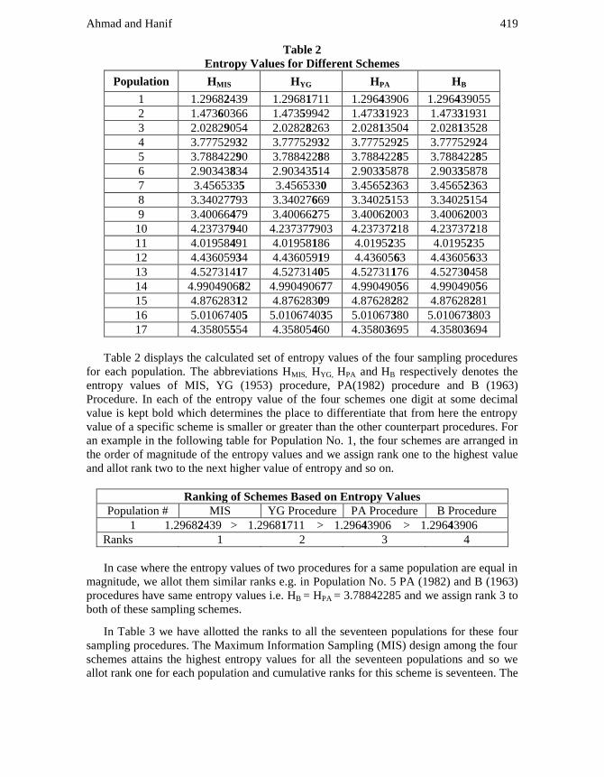
Table 2 displays the calculated set of entropy values of the four sampling procedures

for each population. The abbreviations HMIS, HYG, HPA and HB respectively denotes the

entropy values of MIS, YG (1953) procedure, PA(1982) procedure and B (1963)

Procedure. In each of the entropy value of the four schemes one digit at some decimal

value is kept bold which determines the place to differentiate that from here the entropy

value of a specific scheme is smaller or greater than the other counterpart procedures. For

an example in the following table for Population No. 1, the four schemes are arranged in

the order of magnitude of the entropy values and we assign rank one to the highest value

and allot rank two to the next higher value of entropy and so on.

Ranking of Schemes Based on Entropy Values

Population # MIS YG Procedure PA Procedure B Procedure

1 1.29682439 > 1.29681711 > 1.29643906 > 1.29643906

Ranks 1 2 3 4

In case where the entropy values of two procedures for a same population are equal in

magnitude, we allot them similar ranks e.g. in Population No. 5 PA (1982) and B (1963)

procedures have same entropy values i.e. HB = HPA = 3.78842285 and we assign rank 3 to

both of these sampling schemes.

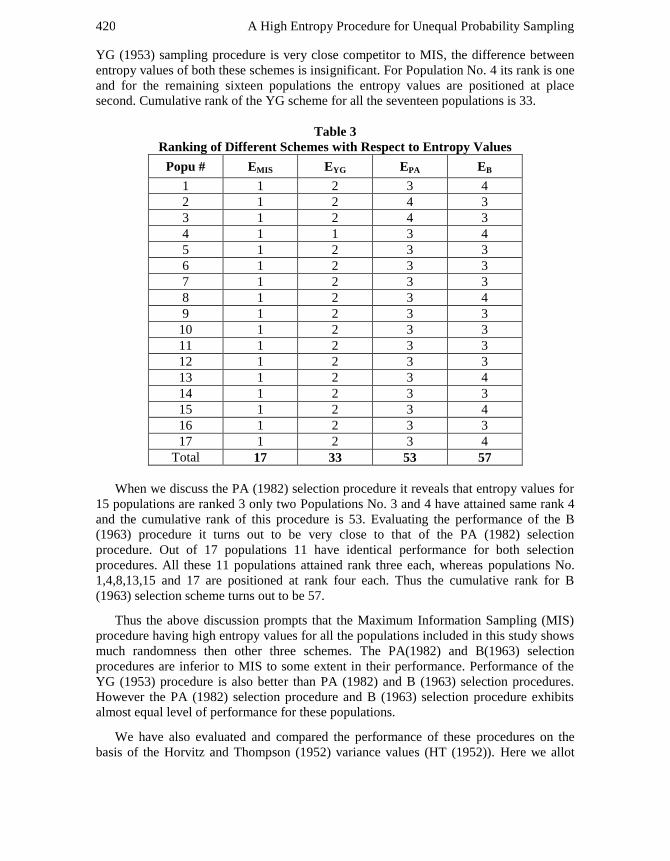
In Table 3 we have allotted the ranks to all the seventeen populations for these four

sampling procedures. The Maximum Information Sampling (MIS) design among the four

schemes attains the highest entropy values for all the seventeen populations and so we

allot rank one for each population and cumulative ranks for this scheme is seventeen. The

A High Entropy Procedure for Unequal Probability Sampling 420

YG (1953) sampling procedure is very close competitor to MIS, the difference between

entropy values of both these schemes is insignificant. For Population No. 4 its rank is one

and for the remaining sixteen populations the entropy values are positioned at place

second. Cumulative rank of the YG scheme for all the seventeen populations is 33.

Table 3

Ranking of Different Schemes with Respect to Entropy Values

Popu # EMIS EYG EPA EB

1 1 2 3 4

2 1 2 4 3

3 1 2 4 3

4 1 1 3 4

5 1 2 3 3

6 1 2 3 3

7 1 2 3 3

8 1 2 3 4

9 1 2 3 3

10 1 2 3 3

11 1 2 3 3

12 1 2 3 3

13 1 2 3 4

14 1 2 3 3

15 1 2 3 4

16 1 2 3 3

17 1 2 3 4

Total 17 33 53 57

When we discuss the PA (1982) selection procedure it reveals that entropy values for

15 populations are ranked 3 only two Populations No. 3 and 4 have attained same rank 4

and the cumulative rank of this procedure is 53. Evaluating the performance of the B

(1963) procedure it turns out to be very close to that of the PA (1982) selection

procedure. Out of 17 populations 11 have identical performance for both selection

procedures. All these 11 populations attained rank three each, whereas populations No.

1,4,8,13,15 and 17 are positioned at rank four each. Thus the cumulative rank for B

(1963) selection scheme turns out to be 57.

Thus the above discussion prompts that the Maximum Information Sampling (MIS)

procedure having high entropy values for all the populations included in this study shows

much randomness then other three schemes. The PA(1982) and B(1963) selection

procedures are inferior to MIS to some extent in their performance. Performance of the

YG (1953) procedure is also better than PA (1982) and B (1963) selection procedures.

However the PA (1982) selection procedure and B (1963) selection procedure exhibits

almost equal level of performance for these populations.

We have also evaluated and compared the performance of these procedures on the

basis of the Horvitz and Thompson (1952) variance values (HT (1952)). Here we allot

Ahmad and Hanif 421

rank one to the smallest or minimum value of variance; rank two is attached to the second

last variance value and ranks are assigned to remaining values in the same pattern. In

Table 4 we have displayed the calculated values of the variances using these procedures

for all the 17 populations and Table 5 displays the ranks assigned to the schemes under

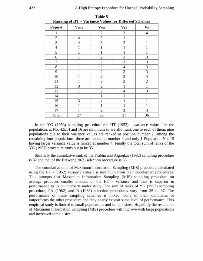
study according to their variance values. The summery data of this table reveals that the

HT- variances values of thirteen populations out of seventeen with Maximum

Information Sampling (MIS) procedure are smaller than their three counterpart

procedures. We allot rank 1 to these populations. The two Populations No. 13 and No. 15

are positioned at rank 3 and the Populations No. 2 and No. 3 are ranked at number four.

Thus the sum of ranks of this sampling procedure turns out to be 27.

Table 4

Horvitz and Thompson Variance Values For Different Schemes

Popu # VMIS VYG VPA VB

1 0.405868 0.407315 0.41463415 0.414635

2 0.288768 0.287748 0.282178 0.282178

3 0.252981 0.252188 0.24810811 0.248108

4 276.14606 276.1447 276.1410 276.1416

5 6373.243 6373.259 6373.319 6373.319

6 24139.243 24145.78 24172.07 24172.07

7 48660.68 48672.01 48713.50 48713.5

8 1866467.6 18666508 1867368.16 1867368

9 9166.601 9167.505 9170.75 9170.747

10 83776.298 83777.05 83779.68 83780

11 55360.58 55383.96 55380.06 55380.06

12 25552.574 25549.02 25536.94 25537

13 18323.626 18323.71 18324.015 18324.01

14 2887.196 2887.224 2887.317 2887.32

15 44054215 44053756 44052254 44052254

16 4591.594 4591.631 4591.75 4591.75

17 1701724 1701737 1701782.67 1701783

A High Entropy Procedure for Unequal Probability Sampling 422

Table 5

Ranking of HT – Variance Values for Different Schemes

Popu # VMIS VYG VPA VB

1 1 2 3 4

2 4 3 1 1

3 4 3 2 1

4 1 1 1 1

5 1 1 1 1

6 1 2 3 3

7 1 2 3 3

8 1 2 4 3

9 1 2 3 3

10 1 2 3 4

11 1 3 2 2

12 3 2 1 1

13 1 2 4 3

14 1 1 1 1

15 3 4 1 1

16 1 1 1 1

17 1 2 3 3

Total 27 35 37 36

In the YG (1953) sampling procedure the HT (1952) - variance values for the

populations at No. 4,5,14 and 16 are minimum so we allot rank one to each of them, nine

populations due to their variance values are ranked at position number 2, among the

remaining four populations, three are ranked at number 3 and only 1 Population No. 15

having larger variance value is ranked at number 4. Finally the total sum of ranks of the

YG (1953) procedure turns out to be 35.

Similarly the cumulative rank of the Prabhu and Ajgonkar (1982) sampling procedure

is 37 and that of the Brewer (1963) selection procedure is 36.

The cumulative rank of Maximum Information Sampling (MIS) procedure calculated

using the HT - (1952) variance criteria is minimum from their counterpart procedures.

This prompts that Maximum Information Sampling (MIS) sampling procedure on

average produces smaller amount of the HT - variance and thus is superior in

performance to its counterparts under study. The sum of ranks of YG (1953) sampling

procedure, PA (1982) and B (1963) selection procedures vary from 35 to 37. The

performance of these sampling schemes is mixed, none of them dominates or

outperforms the other procedure and they nearly exhibit same level of performance. This

empirical study is limited to small populations and sample sizes. Hopefully the results for

of Maximum Information Sampling (MIS) procedure will improve with large populations

and increased sample size.

Ahmad and Hanif 423

ACKNOWLEDGEMENTS

The authors are thankful to Dr. Farrukh Shehzad and referees for significant

suggestions that added value to the manuscript of this paper.

REFERENCES

1. Berger, Y.G. (1996). On sampling with unequal probabilities close to rejective

sampling. SSC Annual Meeting June 1996 Proceedings of the Survey Methods

Section.

2. Brewer, K.R.W. (1963). A model of systematic sampling with unequal probabilities.

Aust. J. Statist., 5, 5-13.

3. Chen, S-X, Dempster, A.P. and Liu, J.S. (1994). Weighted finite population sampling

to maximize entropy. Biometrika, 81, 457-469.

4. Deshpande, M.N., Prabhu–Ajgonkar, S.G. (1982). An IPPS sampling scheme.

Statistica, 36(4), 209-212.

5. Durbin, J. (1967). Design of multistage surveys for the estimation of sampling errors.

Applied Statist., 16, 152-164.

6. Hájek, J. (1981). Sampling from a finite population. New York: Marcel Dekker.

7. Horvitz, D.G. and Thompson, D.J. (1952). A generalization of sampling without

replacement from a finite universe. Journal of the American Statistical Association,

47, 663-685.

8. Hanif, M. and Brewer, K.R.W. (1980). Sampling with unequal probabilities without

replacement: A Review. International Statistical Review, 48, 317-335.

9. Joe, H. (1990). A winning strategy for lotto games? Canad. J. Statist., 18, 233-244.

10. Samiuddin, M. and Asad, H. (1981). A simple procedure of unequal Probability

Sampling. Biometrika, 68(3), 728-731.

11. Samiuddin, M. and Kattan, A.K. (1991). A Procedure of Unequal Probability

Sampling. Pak. J. Statist., 7(3)B, 1-7.

12. Sampford, M.R. (1967). On sampling without replacement with unequal probabilities

of selection. Biometrika, 54, 499-513.

13. Stern, H. and Cover, T.M. (1989). Maximum entropy and the lottery. J. Amer. Statist.

Assoc., 84, 980-85.

14. Shannon, C.E. (1948). A mathematical theory of communication. Bell System

Technology Journal, 27, 623-656.

15. Yates, F. and Grundy, P.M. (1953). Selection without replacement from within strata

with probability proportional to size. Journal of the Royal Statistical Society B, 15,

235-261.