SLAC - PUB - 4320 May 1987

(4

.

AN INTRODUCTION TO ACCELERATION MECHANISMS*

R. B. PALMER

Stanford Linear Accelerator Center, Stanford University, Stanford, California 94305

and Brookhaven National Laboratory, Upton, New York 11973

Table of Contents

Page

1. Introduction ................................

Theorem 1. General Acceleration Theorem ..................

2. Radiation Pressure .............................

A) Nonrelativistic ............................

B) Relativistic .............................

3. A Nonrelativistic Case (the Popderamotive Force) ...............

4. Allow Free Charges (Plasma Beat Wave Acceleration) .............

5. Allow External Magnetic Field B (Inverse Free Electron Laser) .........

6. Allow Finite Refractive Index (Inverse Cerenkov Effect) .............

7. Acceleration Near a Planar e.m. Source (the Grating Accelerator) ........

Theorem 2. Lawson’s Theorem .......................

Grating Accelerator ............................

8. Acceleration Between Planar e.m. Sources (2D Linac) .............

9. Acceleration with Cylindrical Symmetry (Conventinal Iris Loaded Linac Structure) .

Theorem 3. Panofsky Wenzel Theorem .......... ; .........

*Work supported by Department of Energy contracts DE-AC03-76SF00515 (SLAC) and DE-AC02-76C0016 (BNL).

Invited talk presented at the Joint US-CERN School on Particle Accelerators: Topical Course on Frontiers on Particle Beams

South Padre, Texas, October 23-29,1986

2

5

7

7

10

11

15

17

21

23

24

25

27

29

31 c

1. Introduction

We wish to discuss the acceleration of charged particles by electromagnetic fields, i.e., by - fields that are produced by the motion of other charged particles driven by some power source. I It is convenient, from the start, to note that such electromagnetic fields may be separated into

. “near” and “far” fields. The distinction can easily be seen when we look at the form of the fields

generated by a moving point charge. From Jackson’ (i. 675, eq. 14.14):

.

-

where ii is a unit vector from the particle to the observation point and R is the distance. p,p and

7 refer to the motion of the charge at time [t - (R/c)], and e is the electric charge. One notes at

once that the first part of this expression falls as 1/R2, just like any static electromagnetic field; -

it is the “near? field part. The second part falls only as l/R and represents a propagating or

radiating field; it is the “far” field.

Of course, we do not in general use fields generated by a single moving charge. It is thus often

more convenient to look at the possible fields by examining Maxwell’s equations and ‘deducing

the kinds of fields that can satisfy them. Taken from Jackson (p. 218, eq. 6.28) but expressed in

MKS units:

d&t) Vxi?(t) = -7

d,!?(t) Vxiqt) = pcdt

v - i(t) = 9 0 (1.4

g is the space charge density, and p and e are the magnetic susceptibility and dielectric constants

in the medium. 6, is the dielectric constant in free space. Since -any time-varying field can be t x- _T_ represented as an integral of sinusoidally time-varying fields, (by taking a Fourier transform) we --

can write

i?(t) = /

i exp{-iwt}dw (1.5)

i(t) = /

g exp{-iwt}dw 0.6)

2

-

,!? and k are complex and depend on the frequency w. The E’s and B’s satisfy the following

modified Maxwell’s equations. We have now also made the assumption that there are no charges

in the space in which these fields are present.

. T7.i = 0 0.8)

v.A?z = 0 (1.10)

From vector algebra (see for instance, inside the front cover of Jackson) we can write

vi = V.(V.i)-Vx(Vxi).

-

From Eq. (1.10)

from Eq. (1.7)

vx3L0,

vxi=iwii,

-

so

and from Eq. (1.9)

v$ = -iwv x i )

vxi = --iwpei

which then gives us the wave equation:

v2i = -pew21k (1.11) -

A similar calculation for I3 gives us

v2ii = --j.4EW2i. (1.12)

All solutions to these equations can be expressed as sums of waves of the form

a& = I30 exp{i(&.?-wt)} , . -

x- _P_ i = Bo exp{i(i;: -f-wt)} .

(1.13) r,

If L is a real vector, i.e., if

i+=k,-z+ky-y+k,.r, (1.14)

then these equations represent traveling waves moving in the direction of the vector i at a velocity

equal to w/lkl = l/G. Since j.4,.5, = 1/c2, by definition, where c equals the velocity of light,

3

we see that the wave velocity is c/N, where the refracted index N = dm. Substituting

Eq.(1.13) into Eqs. (1.8) and (l.lO), we obtain

- &4 = 0, (1.15)

. &i = 0, (1.16)

These show us that the waves that we are discussing are transversely polarized (again on the

assumption that the vectors E are real). Finally, using Eq. (1.7), we can relate the B fields to the

E fields, and obtain

which shows us that the B fields and E fields are perpendicular to one another and that the - magnitude of the E field is equal to the magnitude of the B field times c. -

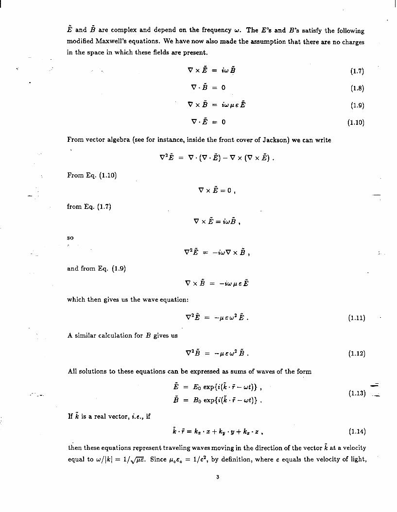
Thus we have found that solutions to Maxwell’s equations in a space with no free charges

include solutions that are plain, parallel, transversely polarized waves with a velocity of c/N,

where N is the refractive index (see Figure 1).

Direction of Wove Propogotion

5-a-l 5779Al

Figure 1

We will see later that these are not the only solutions. i need not be a real vector, and if complex, the waves represented by Eqs. (1.13) and (1.14) contain exponentials. These solutions fall in amplitude at distances which are far from any changes and thus cannot exist “FAR” from

such sources. They are referred to as “NEAR” fields (see Sections 7-9). For -the moment we will

consider only “FAR” fields (see Figure 2). 4 --

5,79A2

Figure 2

4

.

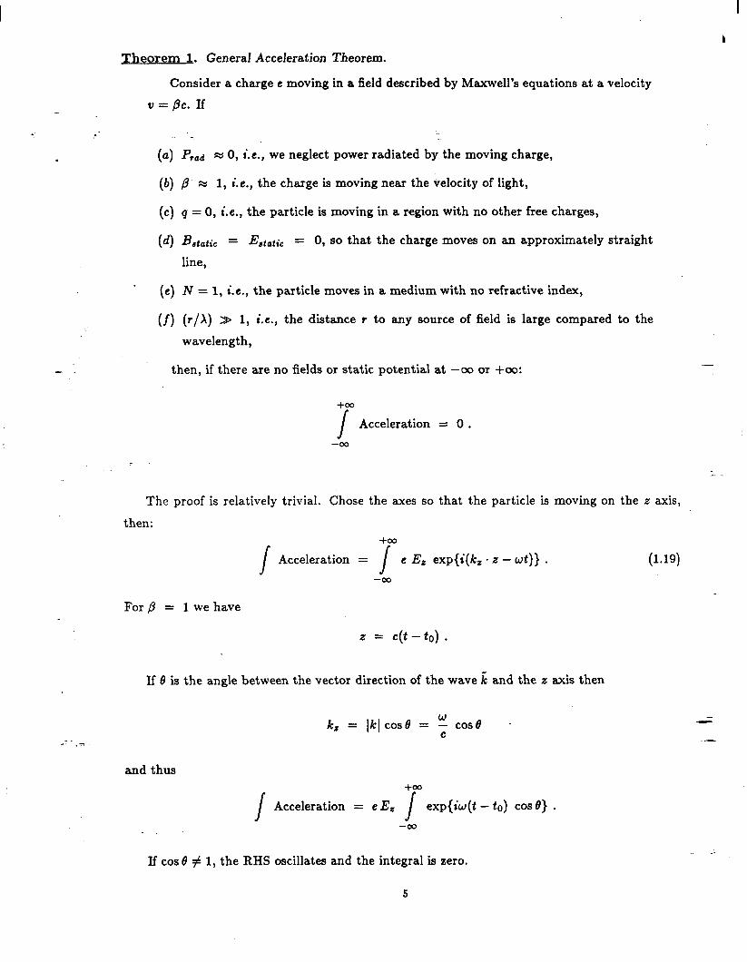
Theorem 1. General Acceleration Theorem.

Consider a charge e moving in a field described by Maxwell’s equations at a velocity

v = pc. If

(‘=) Prod = 0, i.e., we neglect power radiated by the moving charge,

(b) P = 1, i.e., the charge is moving near the velocity of light,

(c) q = 0, i.e., the particle is moving in a region with no other free charges,

(d) Bstatic = Eatcrtic = 0, so that the charge moves on an approximately straight

line,

. (e) N = 1, i.e., the particle moves in a medium with no refractive index,

(f) (r/X) 29 1, i.e., the distance t to any source of field is large compared to the

wavelength,

- then, if there are no fields or static potential at -oo or +oo:

+w

J Acceleration = 0 . -w

The proof is relatively trivial. Chose the axes so that the particle is moving on the z axis,

then: +w

J Acceleration = J e E, exp{i(k, . z - wt)} . (1.19)

-w

For p = 1 we have

z = c(t - to) .

If 6’ is the angle between the vector direction of the wave k and the z axis then

k, = lkl case = ; cosd

and thus +w

J Acceleration = e& J exp{iw(t - to) COST} . -w

If cos 0 # 1, the RHS oscillates and the integral is zero.

5

A

-

If cos 8, = 1, then the wave is propagat ing in the z direction and from the transverse polar-

ization condit ion [Eq. (l.lS)] Et = 0. Thus in all cases, acceleration is zero. No playing with a

focus or phase plates or holograms can change this.

‘ In the following sections we will deal with acceleration that occurs when we relax one of the

condit ions listed above. .

s-- -

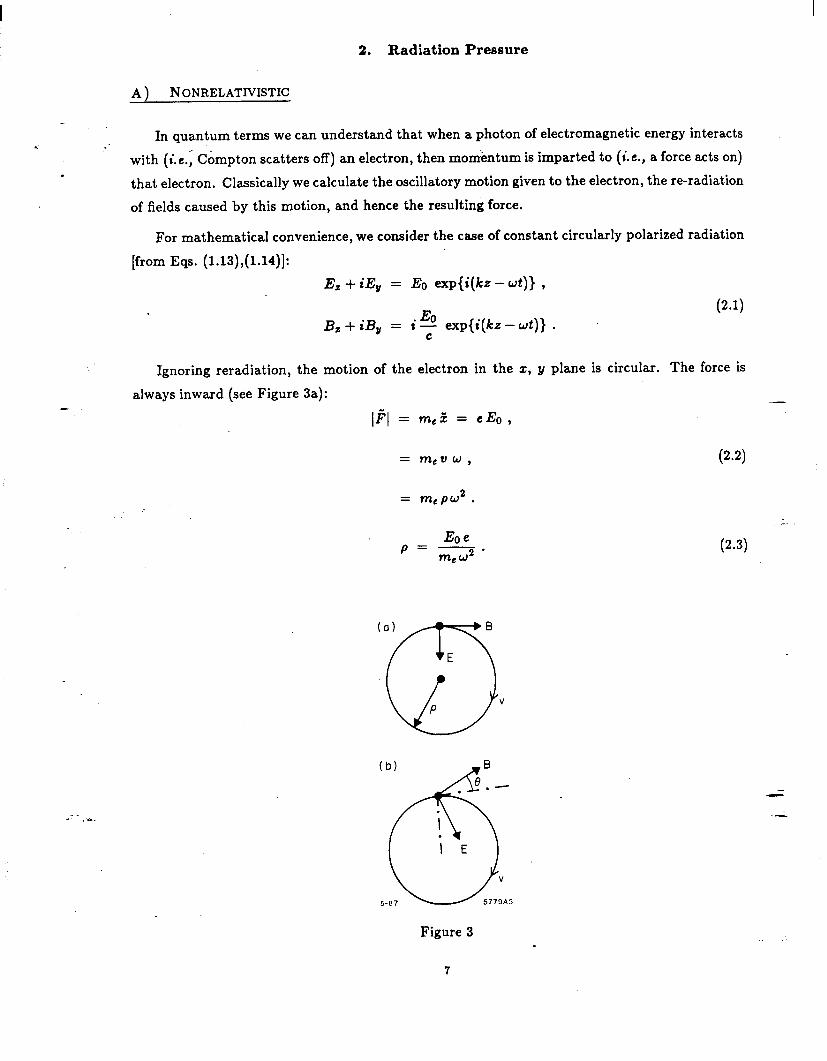
2. Radiation Pressure

A) NONRELATIVISTIC

-

.

In quantum terms we can understand that when a photon of electromagnetic energy interacts

with (Le., Compton scatters off) an electron, then momkntum is imparted to (i.e., a force acts on)

that electron. Classically we calculate the oscillatory motion given to the electron, the re-radiation

of fields caused by this motion, and hence the resulting force.

For mathematical convenience, we consider the case of constant circularly polarized radiation

[from Eqs. (1.13),(1.14)]:

Ez + iE, = E. exp{i(kz - wt)} ,

(2.1) B, + iB, = .Eo t c exp{i(kz - wt)} .

Ignoring reradiation, the motion of the electron in the z, y plane is circular. The force is

always inward (see Figure 3a): - Fl = me2 = CEO,

= m,vw, (2.2)

= mcpw2.

Eoe p=---&-p

e 2 P-3)

(CA) B

E

cl v P

C

Figure 3

7

-

FOR EXAMPLE: for the kind of field generated by a 1 cm-long focus of a 1.7 TW CO2 laser,

we might have:

EO fit 100 GV/m,

e w 1.6 x lo-*’ C ,

me m 9.1 x 10m31 kg,

then:

p w .Spm.

This circular motion will radiate a power P (see Jackson, p. 665):

P 2 e2

rad = - - r”(q2 & , 3 c3 0

or, if nonrelativistic, and substituting

I eEo 2= , me

P rad M 2 e*Ei 1 iGFxG? e 0

(24

- (2.5)

(2.6)

There are several ways of deriving the forward force on the electron:

(1) by considering the interference of incoming and radiated fields;

(2) by using energy and momentum conservation,

(3) by noting the consequences of a phase slip.

I will use the latter. By energy conservation a phase slip 6 must exist between the electron

motion and the incoming field (see Figure 3b). The power given to the electron from the field is,

-

P received = Eoeu sin+, (2.7) -, --

where

eEo u - = mew ’

and

P rce = &ad I

8

(2.8)

so using (2.6):

-

Eg e2 2 e*Et 1 sin4 = - - - mew 3 m2c3 47rE, ’

6

sinfj = .

which, using the definition of the classical electron radius te,

r e = e24r E, me c2 ,

gives 2 w

sinqi = -Te-. 3 c

A

(2.9)

(2.10)

FOR EXAMPLE: for the above example

- w = 188 x 10” set-l . ,

c = 3 x lo* m/set ,

re = 2 8 x lo-” m . ,

sin q5 m 1.2 x 10-g .

which is a very small angle c$ !

Referring again to Figure 3b, we see that there is now a finite force in the z direction

(2.11)

Eo =e-usinf$. C

e& u - = T?leW ’

so

FE = eEo eEo 2 w ---re-

C Q&W3 C’

FE = f (Eo e)2 z ??leC2 ’

(2.13)

9

which is the expression for the nonrelativistic radiation pressure. It may be compared with

the instantaneous radiation force Eo e:

Fz 2 fF = - = Eoe zEoe%.

.~ me C2 (2.14)

which increases as the field EO increases, but even for our rather high power laser example, this

fraction is very small.

Eo = 100 GV/m, (2.15)

fF = 3.6 x 10-l’ .

It is clear that radiation pressure is not a practical means of accelerating particles.

B j RELATIVISTIC

- It might appear from Eq. (2.4) that if -y is large, the radiation might also become large

(P,,#%y*). But in this case we have to consider also the force on the moving electron from the B y field of the wave

meja = J’ = Fe + FB ,

= eEo-eBou

= eEo --e&P,

= e-h (l-P),

So for 7 > 1, 2

p=-ze2* c$ 1

3 7’ ( > 47r&, ’

and we see that radiated power, and thus force, has not increased.

Thus for all practical caseS the first assumption of Theorem 1 is satisfied.

(2.16)

(2.17)

10

A

3. A Nonrelativistic Case (the Ponderamotive Force)

-

.

We have seen in Sec. 2 that a uniform electromagnetic wave induces only small forces on an

electron. The same is not true for a time varying field.

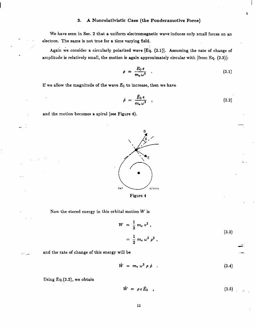
Again we consider a circularly polarized wave (Eq. (2.1)]. Assuming the rate of change of

amplitude is relatively small, the motion is again approximately circular with [from Eq. (2.3)]:

P Eoe =-.

me W2

If we allow the magnitude of the wave Eo to increase, then we have

.

b+$, e

and the motion becomes a spiral (see Figure 4).

Figure 4

Now the stored energy in this orbital motion W is

W = r me u2, 2

1 = - m, w2 p2 , 2

and the rate of change of this energy will be

FV = meW2p/j .

Using Eq.(3.2), we obtain

I+ = pei$ ,

(34

(3.2)

(3.4)

(3.5) _-

11

-

c

I L

which must equal the energy given to the electron. Again, as in Sec. 2, a phase 4P must &v&p

(see Figure 4) so that such an energy gain can take place:

vir = Eoeu sinr&, ,

= Eoewp sin& . (3.6)

.

Equating Eqs. (3.5) and (3.6) gives

P e i0 = Eoewp sin4p,

so .

Eo 1 sin&= -.; . Eo P-7)

-

Unlike the radiation pressure phase angle of Eq. (2X), t$,, can be large. &, is of the order of .

the reciprocal of the number of cycles over which the amplitude charge occurs. -

As in the radiation pressure case, this phase angle produces a finite force in the z direction:

Eo =- C

e u sin & ,

Eoe = -pw sin&, C

so with Eq. (3.7):

Fz = Eoe I& 1 CPwE;’

0

Fz = e&:,

and the ratio of this to the radial force Eo e:

FE fF = hoe =

1 &!P.- c Eoe

.- -1. using Eq. (3.1)

. fF = & = = .

mw2c

(3.8) 1.

(3.9) -

(3.10)

12

Figure 5

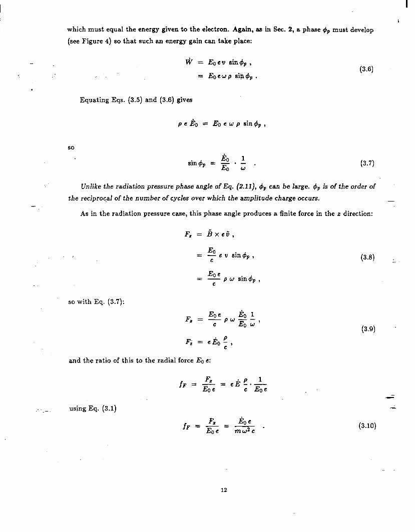
As an example of time varying fields, we consider the beat of two waves, each with amplitude

Eo, at frequencies wr and wp, where WI ti ~2. The fields will be as shown in Figure 5. The resultant time varying amplitude will be:

Eo(t) = 2Eo sin [(wp - wr) t] , (3.11)

and the maximum rate of change of this amplitude:

- .

&ma, = 2~90 (W2 - WI) .

The resulting maximum accelerating force [using Eq. (3.9)] is

F zmaz = 2eEo (W-WI) : . (3.13)

and the ratio of this force to the maximum radial force (2e Eo) is

eEo wa-wl fF=E w2 . e

As an example, we consider the beat from two lines of a CO2 laser where

W2 - Wl e 3% W

Eo = 100 GV/m = 10” V/m

w = 1.9 X lo’* set-l

fF = 3 x lo-3

(3.12) 7

(3.14)

which is not so negligible!

Fz = 1 GV/m

13

The acceleration, unfortunately does not continue indefinitely. The maximum velocity

achieved t

Vmaz = J $dt , 0

from Eq. (3.9)

2ep d& F,=-- C dt ’

from Eq. (2.3)

CEO P - =

mcwa ’

t v(t) =. J 2e CEO dEo --

C - dt , mec2 m, w2 dt

0

v(Eo) = (&)2 2 f Eo dEo 0

Vmaz :+

2 -= .

C

(3.16)

. (3.17)

For our example,

Eo = 100 GV/m

w = 1.88 x 10” set-’

me = 9 1 x lo-= k . I3

e = 1.6 x 10-l’ C

c = 3 X lo* m set-l

Vmaz -= C

%?I I o.1 .

C

So that acceleration can even reach relativistic velocities with plausible laser power levels. --

However it is clear from Eq. (3.16) that integrating from any point with EO = 0 to any other

point with Eo, the net acceleration is zero. This example suggests, although it does not prove,

that condition (b) is not in fact required for the result of Theorem 1 to be correct.

14

I

A 4. Allow Free Charges (Plasma Beat Wave acceleration)

The Ponderamotive force (see Sec. 3) can be used to induce perturbations in an otherwise

uniform distribution of charges, and the “static” fields generated by these perturbations can be

used to accelerate particles. This idea was proposed by Willis for charges in a dense beam.2 More . realistically, Dawson proposed the perturbation of charges in a plasma.3 In this case he explicitly

proposed that beat waves be used (as discussed in Sec. 3) and that the resulting oscillations in

electron plasma density be enhanced by selecting a plasma whose plasma frequency is equal to

the beat frequency, i.e.,

Wl -w2 = wp . (4.1)

In this case the amplitude of the plasma oscillations will increase until losses or nonlinearities

overcome the amplification provided by the beat wave. The nonlinearities will clearly stop the

process before the amplitude is such as to cause the plasma density, at its oscillating minima, to

become zero. -

To examine the magnitude of acceleration that we may expect, we return to Maxwell

[Eqs. (1.1) to (1.4)). If we assume that there is a solution in which the excess change density q is

also periodic in t and z, i.e., a plasma wave with

g = pe = paexp{i(k,z-wt)},

E = EO exp{i(k, z - wt)} .

Then substituting in Eqs. (1.1) to (1.4) f or small a, one obtains a solution if

p. e2 { >

112 UP= em ,

0 c

(4.2)

(4.3)

which frequency is defined as the “plasma frequency.”

The amplitude a cannot be greater than 1. If it were, the electron density would have to be

negative. In practice, nonlinearities will limit a to = l/10.

From Eq. (1.4) we have

_ _ .3. V.E = p . to

That is,

= t a p. exp{i(k,z - wt)} .

0

15

Differentiating E from Eq. 4.3, we get

Eok, = %a,() . - G

‘ = - Substituting for po using Eq. (4.4), and for kz using & = w,,/c:

Eo = wpm,ca

e I

which gives the amplitude of longitudinal acceleration as a function of the wave density amplitude

a. Clearly, higher fields are possible at higher plasma frequencies.

. For an example consider the beat wave between two CO2 laser frequencies 10% apart,

then

WP = 1.88 x 1o13 (A, = 100 pm)

- me = 9.1 x 10 -31 kg

c = 3x10* msec-1

e = 1.6 x 10-r’ C

po = 3.8 x 1O22 m (3.8 x 10’6cm-2) .

If

then

Eo = 3.2 x 10’ (3.2 GeV/m) .

Thus we see that with a quite reasonable plasma density, very high acceleration gradients are

possible. Of course plasmas are complicated and the efficiency of driving the beat wave will not

in general be 100%. Much study is being devoted to this mechanism.’

Note also that such a plasma wave can be excited by a bunch of low-ener.gy particles passing

through the plasma. The mechanism is then known as a “plasma wake accelerator.“5 2

16

5. Allow External Magnetic Field B (Inverse Free Electron Laser)s

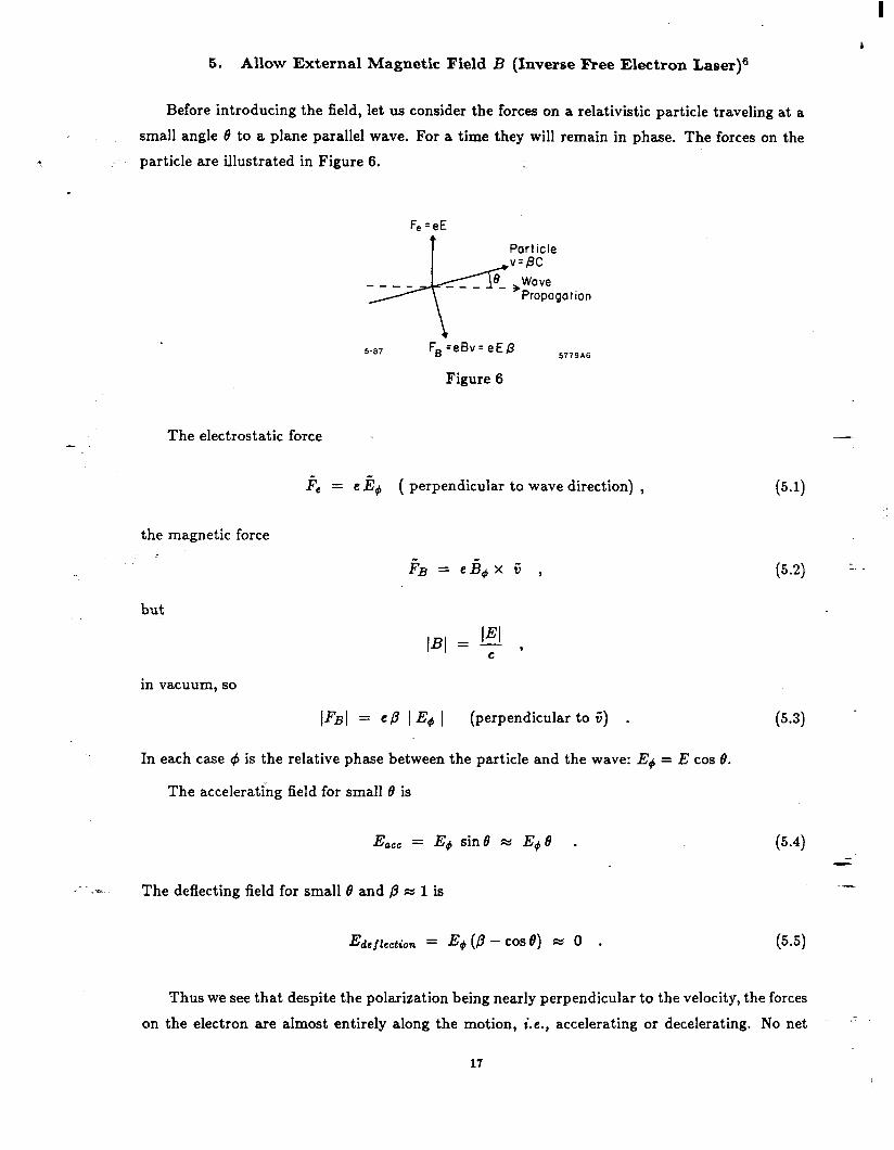
Before introducing the field, let us consider the forces on a relativistic particle traveling at a

‘ small angle 8 to a plane parallel wave. For a time they will remain in phase. The forces on the

; - particle are illustrated in Figure 6. .~

.

+

Particle v=BC

8 ---- --- _ ,Wave Propagation

5-87 FB =eBv = eEP

Figure 6

5779A6

- The electrostatic force

Fc = e &, ( perpendicular to wave direction) ,

the magnetic force

FB = eE$x C , (5.2) -. -

(5.1)

but

in vacuum, so

p3I = F ,

[FBI = ep I E+ I (perpendicular to C) . (5.3) .

In each case # is the relative phase between the particle and the wave: Ed = E cos 8.

The accelerating field for small B is

E ace = E# sin8 M Ede . (54

_ ..=. The deflecting field for small B and /3 ti 1 is

E de f lcction = E@-COSB) m 0 . (5.5)

Thus we see that despite the polarization being nearly perpendicular to the velocity, the forces

on the electron are almost entirely along the motion, i.e., accelerating or decelerating. No net se

17

-

c

acceleration will occur because as the phase slips, acceleration and deceleration will alternate.

Let us estimate this rate of slip. Let z be the direction of wave propogation. Then:

v, (wave) = c ,

V, (particle) = C~%S e .

Their phase q5 will slip by 2~ in a distance:

A 2x

=z,

where

K+&) ’ K=k(;++) .

-

If we assume e2/2 B 1/2q2 then 2x

Amp.

(5.6)

WI

_ For a distance A/2 we can have acceleration, then it will reverse. Over a long distance there -. - will be no net acceleration, How can we overcome this? Suppose after each distance A/2 we have

a magnet that reverses the sign of 8 (see Figure 7), acceleration will then continue indefinitely. _

/- \ ,: E ,

Figure 7

_ _ __. Since the acceleration is proportional to 0, we wish to maximize the amplitude of the zig-zag; -

with a fixed B, this is achieved by having a field everywhere but alternating its sign with an

appropriate period. Such magnets are known as wigglers.

A more elegant (and easier to calculate) solution is to use a “helical field;” i.e., a field that

remains transverse but whose direction rotates about the axis. It is the field generated by a

winding of two interleaved helical wires, carrying opposite currents. The motion of a charged .: particle in such a field will also be a helix with constant angle 0.

18

The helical field is, given by

B,+iB, = I30 exp{iKz} .

’ The force on the particle is then

Fz + iF, = ievBo exp(iKz} ,

dpz . dpu =z+‘z,

so

Pz+ipv = J ie v Bo exp{iKz} dt ,

evBo = - exp{iKz} , K dz z

(5.10)

(5.11)

(5.12)

- and evBo

PI = - Kdz ’ aF

(5.13)

w !$ (for small e) .

The transverse momentum is a constant, with its direction rotating about the axis (i.e., a helix).

The helix pitch angle B is then:

Now, from Eqs. (5.6) and (5.9)

Substituting in Eqs. (5.14) gives

e

and from Eq.. (5.4)

(5.14)

(5.15)

Ea = E~~cos~

so

E,(mas)=EoO . *

19

For example, with a powerful CO2 laser one might have

X = lOpm,

B = 1 Tesla

me = 9.1 x 10m31 kgm ,

c = 3 x lo* m set-I

E. = 10” eV/m (100 GV/m) ,

then for

7 = 100 (50 Mev) , 8 = 1.2 x 10e2 , -Ea = 1.2 GV/m ,

7 = lo5 (50 GeV) , B = 1.2 x 10v3 , E, = .12 GV/m .

Thus we see that we can obtain good acceleration at low energies but it becomes less attractive - as the energy goes up. In addition, C. Pellegrini7 has pointed out that synchrotron radiation

effectively limits the usefulness of the method above a few hundred GeV.

20

&

6. Allow Finite Refractive Index (Inverse Cerenkov Effect)

This mechanism was first discussed and subsequently demonstrated by R. Pamel.* As in

Sec. 5, we can start by considering the interaction of a relativistic particle with a plane wave

.-^ traveling in- nearly the same direction. As in Eq. (5.4), the accelerating field is

. E ace = E$ sine ) (6-l)

where 8 is the angle between the particle and traveling plane wave and Ed = EO co8 8, where 4 is

the relative phase between the particle and that wave. The deflecting field will again be

Edcf = E&3 - COSB) (

which for /3 fit 1 and 0 small is negligible.

The phase 4 will be given by -

($ = +,+w (

Nz;ose - t >

;

(6.2)

-

(6.3)

where N is the refractive index of the medium. If N # 1 then we can arrange to keep the phase

rj constant by setting:

The accelerating field is then

‘NcosB=l . (64

E act = EO sine = . (64

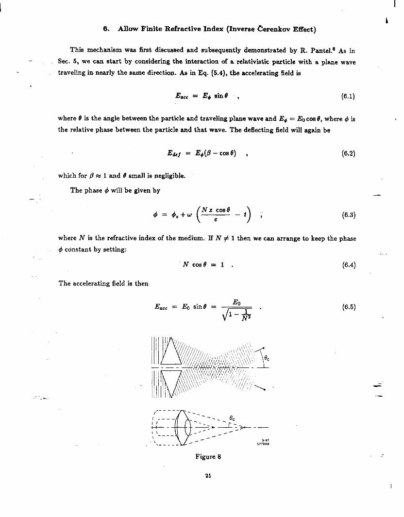
Figure 8

Clearly, this could be a very efficient and simple mechanism if N could be made reasonable

large. Unfortunately, a large N implies a high density of gas and that will (1) break down at

lower field and (2) cause Coulomb scattering of the beam. How serious these are would depend - on the application.

4 =- A more-. “e&ient” geometry than that of a plane Gave is obtained at an “axicon” focus.

. This is the field obtained by adding waves, each at a fixed angle 0 to the beam axis, but at all

different azimuthal angles. It is obtained by passing a plane parallel wave through an “axicon” lens

(see Figure 8). Such a field is also present in a circular waveguide excited in the TE,, mode.

The fields are well known in this case, and are described by Bessel Functions of the first kind

(see Jackson,l p. 367).

22

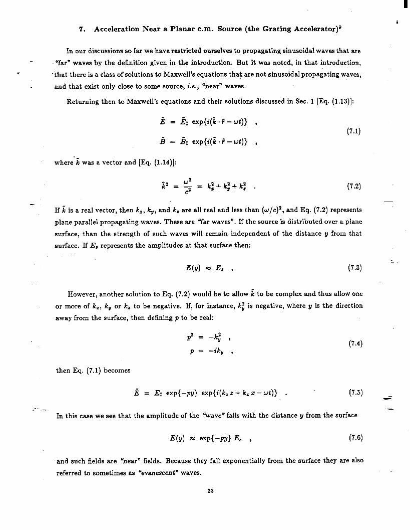
7. Acceleration Near a Planar e.m. Source (the Grating Accelerator)g

In our discussions so far we have restricted ourselves to propagating sinusoidal waves that are

“far” waves by the definition given in the introduction. But it was noted, in that introduction,

.=that there is a class of solutions to Maxwell’s equations that are not sinusoidal propagating waves,

. and that exist only close to some source, i.e., “near” waves.

Returning then to Maxwell’s equations and their solutions discussed in Sec. 1 [Eq. (1.13)]:

i

i-2 = & exp{i(k+-wt)} , (7.1)

ii = ii(-) exp{i(k .i-wt)} ,

where-k was a vector and [Eq. (1.14)]:

p = W2

c2 = k; + k; + kz . (7.2)

- - If i is a real vector, then k,, k,, and k, are all real and less than (w/c)~, and Eq. (7.2) represents

plane parallel propagating waves. These are “far waves”. If the source is distributed over a plane

surface, than the strength of such waves will remain independent of the distance y from that

surface. If Ed represents the amplitudes at that surface then:

.E(Y) - E, , (7.3) -’

c However, another solution to Eq. (7.2) would be to allow k to be complex and thus allow one

or more of k,, k, or kz to be negative. If, for instance, ki is negative, where y is the direction

away from the surface, then defining p to be real:

p2 = -k; ,

P = -ik, , (7.4

then Eq. (7.1) becomes

i = Eo exp(-py} exp(i(k, z + k, z - wt)} . (7.5) G

In this case we see that the amplitude of the “wave” falls with the distance y from the surface

E(Y) = exp{-m) E, , (74

and such fields are “near” fields. Because they fall exponentially from the surface they are also

referred to sometimes as “evanescent” waves.

23

I

For convenience let us consider waves traveling along the z direction, i.e., k, = 0:

j!? = &, exp{-p,,} exp{i(k, z - wt)} , -

k,2 = i -

(7.7) (7.8)

. Substituting into Eq. (1.10) gives

-E,ip+E,k, = 0 ,

and thus .

Ez = FE,, . (7.9) L

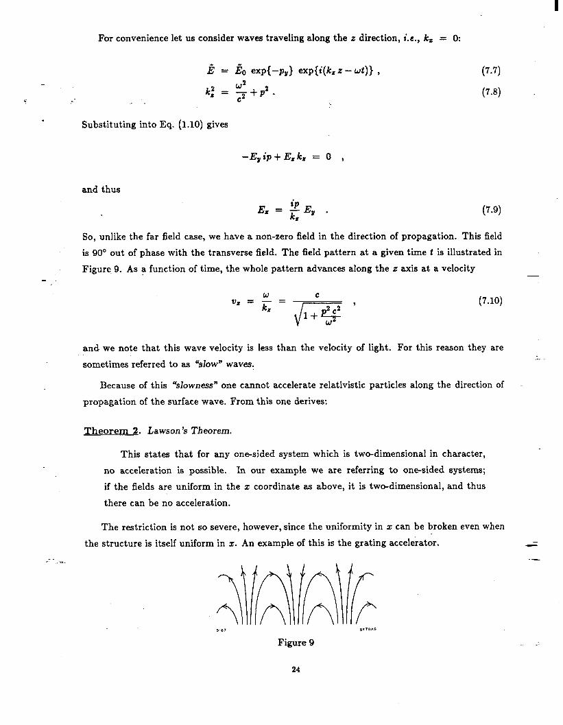
So, unlike the far field case, we have a non-zero field in the direction of propagation. This field

is 90’ out of phase with the transverse field. The field pattern at a given time t is illustrated in

Figure 9. As a function of time, the whole pattern advances along the z axis at a velocity - -

(7.10)

and we note that this wave velocity is less than the velocity of light. For this reason they are 1.

sometimes referred to as “slow” waves.

Because of this ((Slowness” one cannot accelerate relativistic particles along the direction of

propagation of the surface wave. From this one derives:

Theorem 2. Lawson’s Theorem.

This states that for any one-sided system which is two-dimensional in character,

no acceleration is possible. In our example we are referring to one-sided systems;

if the fields are uniform in the z coordinate as above, it is two-dimensional, and thus

there can be no acceleration.

The restriction is not so severe, however, since the uniformity in z can be broken even when

the structure is itself uniform in ZC. An example of this is the grating accelerator. C

Figure 9

24

GRATING ACCELERATOR

In a grating accelerator, slow waves are excited on the surface of a periodic structure in such

s - a way that the direction of propagation of the waves are oriented diagonally across the surface

from both sides. The two.sets of waves generate a periodic wave pattern that is periodic in both . P and z, i.e., k, and k, are finite and real; k, is imaginary leading to an exponential fall-off of

field away from the grating surface. For acceleration in the z direction we require

since

W2

c2 = k: + k; + k; ,

thus -

k; w -k; = p2 ,

and the field on a particle traveling at the velocity of light (z = ct) is

Ez = Eo exp{--P,} exp(i(4, +k,z)} , (7.11) L.

where

f$, =z,--ct, .

_.

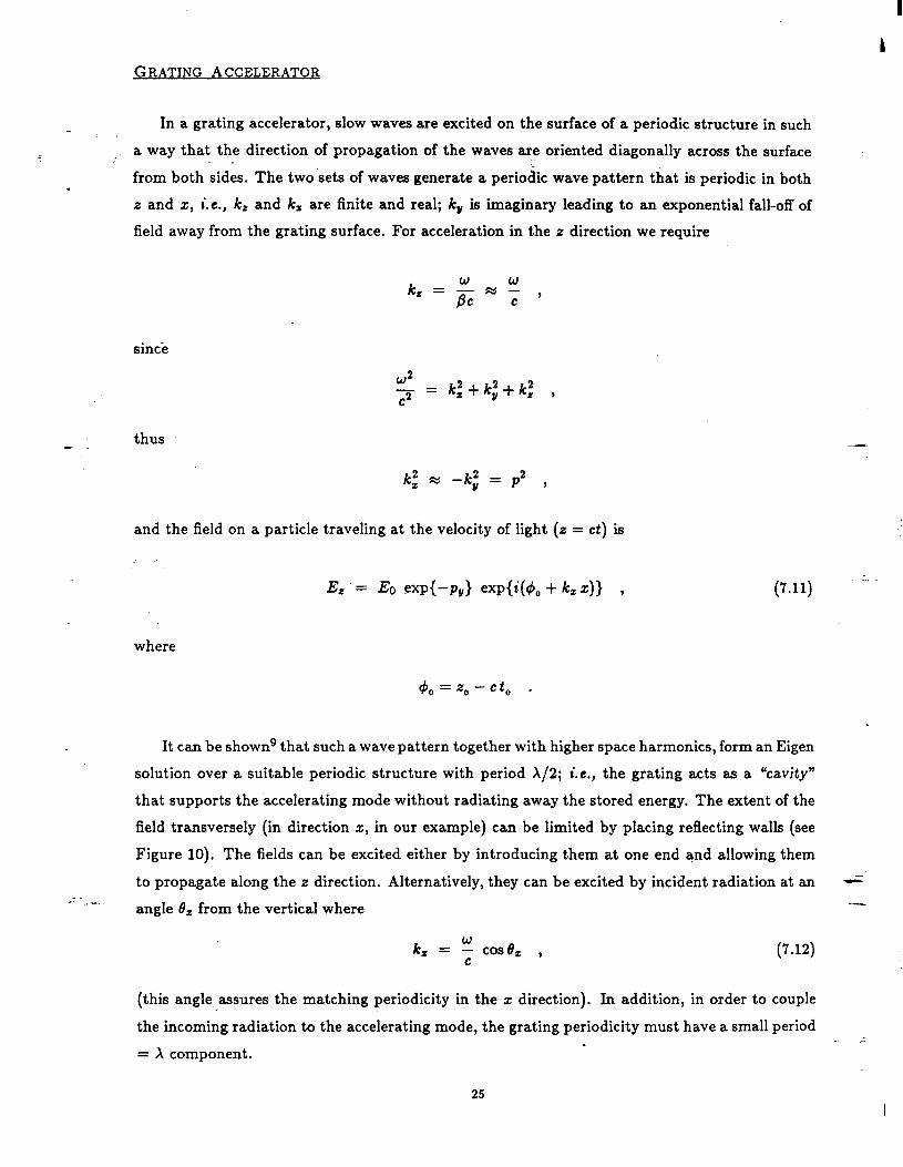
It can be shown9 that such a wave pattern together with higher space harmonics, form an Eigen

solution over a suitable periodic structure with period X/2; i.e., the grating acts as a “cavity”

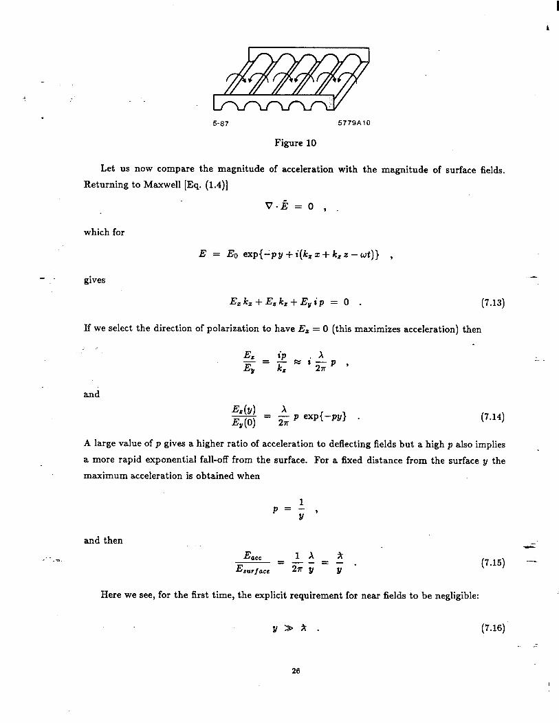
that supports the accelerating mode without radiating away the stored energy. The extent of the

field transversely (in direction x, in our example) can be limited by placing reflecting walls (see

Figure 10). The fields can be excited either by introducing them at one end and allowing them

to propagate along the z direction. Alternatively, they can be excited by incident radiation at an 2

angle kJz from the vertical where

k,+ose, , (7.12)

(this angle assures the matching periodicity in the z direction). In addition, in order to couple

the incoming radiation to the accelerating mode, the grating periodicity must have a small period .

= X component.

25

. 5-87 5779AlO

Figure 10

Let us now compare the magnitude of acceleration with the magnitude of surface fields.

Returning to Maxwell [Eq. (1.4)]

v.J!? = 0 (

which for

E = Eo exp{+ y + i(k, z + kz z - wt)} ,

- gives

Ezkz+Ezk,+E,ip = 0 .

If we select the direction of polarization to have Ez = 0 (this maximizes acceleration) then

and

(7.13)

(7.14)

A large value of p gives a higher ratio of acceleration to deflecting fields but a high p also implies

a more rapid exponential fall-off from the surface. For a fixed distance from the surface y the maximum acceleration is obtained when

and then _ E _ _T. act 1x x .

E --=-.

6ULIfOCC =27ry y

2

(7.15) -,

Here we see, for the first time, the explicit requirement for near fields to be negligible:

y>>x. (7.16)

26

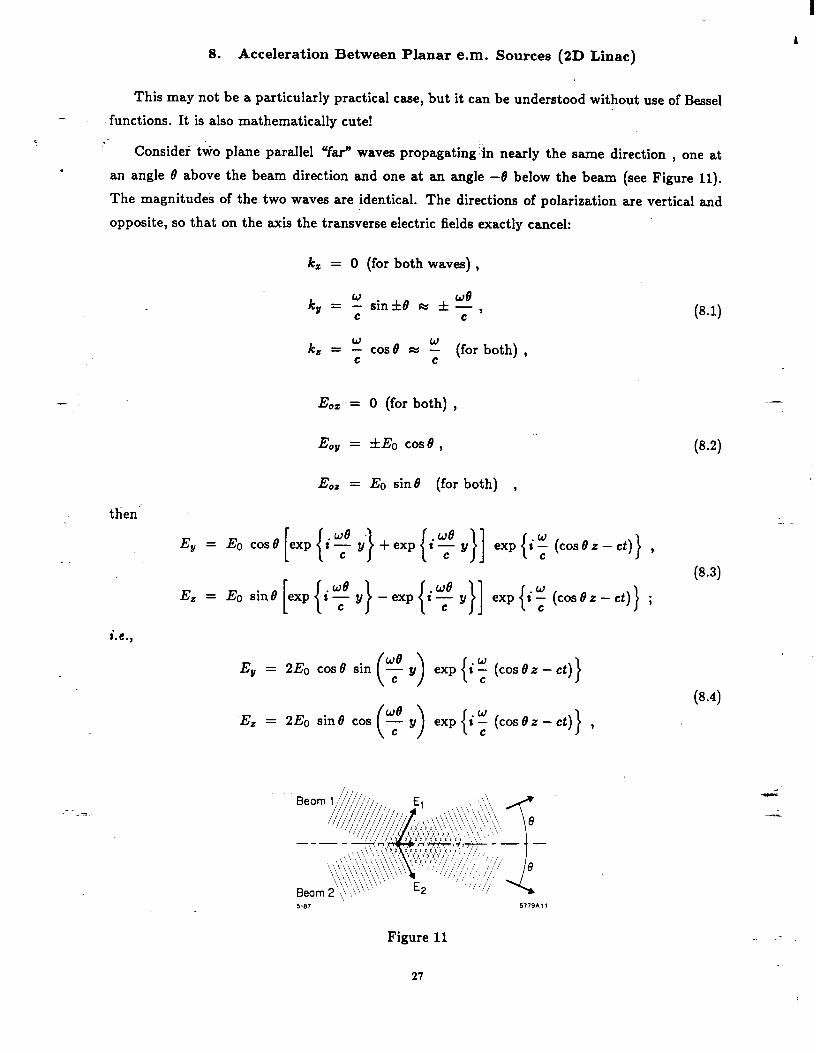
h 8. Acceleration Between Planar e.m. Sources (2D Linac)

This may not be a particularly practical case, but it can be understood without use of Bessel - -functions. It is also mathematically cute!

. Consider ttio plane parallel “far” waves propagating% nearly the same direction , one at

an angle 8 above the beam direction and one at an angle -8 below the beam (see Figure 11). The magnitudes of the two waves are identical. The directions of polarization are vertical and

opposite, so that on the axis the transverse electric fields exactly cancel:

k, = 0 (for both waves) ,

- E 02 = 0 (for both) ,

k, = 5 we C

sin&B fi: f-, C

k, = w case M w C

c (for both) ,

Eo, = rtEo cos e ,

(84

(84

then’

E 02 = EO sin8 (for both) ,

E, = Eo case exp i [ { $,)+exp{iG y}] exp{it (cOseE-ct)} ,

Ez = Eo sine exp i@y [ { c }-exp{iT y}] exp{it (cosez-ct)} ; (8*3)

i.e.,

E, = 2Eo case sin-($ y) exp{iF (cosdz-ct)}

(84 Ez = 2Eo sin8 cos($ y) exp{i: (cosez-et)} ,

Figure 11

27

I

which for 8 --) 0 and 2Eo 8 -+ A0

-

i

E, e Ao ty exp{it (z--t)} ,

Ez fi: A0 exp it (z 1

- ci)} .

(8.5)

.

Here we see that the accelerating field will remain in phase with the particle and need not go

to zero (Eo went to 00, as 8 -t 0, but the observed fields can remain finite). We note moreover

that the accelerating field is independent of transverse position z or y. However, the transverse

field E, rises linearly with y.

If the fields are generated at two surfaces at fy, then

&cc (0) 1x x p=-=--=-. Ed(Y) :Y 2AY Y

(8.6)

- We note that this is the same relation as found for the optimized planar grating accelerator -y

[Eq. (7.15)]. Although we started with two far fields we have, by taking the limit 8 -+ 0 obtained

a “near” field solution.

28

9. Acceleration with Cylindrical Symmetry (Conventional Iris Loaded Linac Structure)

- As in Sec. 8 we can again derive the near field solution by starting with.a far field case and

taking a limit. We start with the fields discussed in Sec. 6; i.e., the inverse of Cerenkov fields i

(see Figure 8). These fields would be formed by taking the two interfering beams of Sec. 8 and . rotating about the axis. Beams are approaching the axis at fixed angles 0 to that axis, but from

all azimuthal directions. The fields that result cannot be simply written down, since they involve

infinite sums, but they can be written in terms of Bessel functions.

In general the fields in an axially symmetric case can be represented as sums of transverse

electic (TE) and transverse Magnetic (TM) modes. Since only the TM modes contain accelerating

fields, we will consider only these. With a along the cylindrical axis, p perpendicular to that axis

and fI circumferential about it [from Jackson,l p. 367, eq. (8.117)]

EE = Eo Jo(pr) - exp{i(h - wt)) ,

E, = -E. exp (i(k, 2 - wt)) ,

Bd = f Jl(P7) * exp {i(k* a - wt)} .

: (Note that we have exchanged E with B to obtain the TM case; the reference being for TE.) I..

In the above 7 is not the relativistic parameter but:

W2 r2 = c2 - k; ,

k, = w c0se , C

P-2) thus

W 7 = ; sine ,

where 8 is the angle between the incoming plane parallel waves and the axis (as in Sec. 8).

Thus

Ez = EO JO (f sine) . e~p {i(kz z - wt)} , NZ

Ep = -Eo & 51 (f sine) .exp{i(k,z- wt)} , (9.3)

cB4 = Eo& 51 (f sine) sexp{i(k,z-wt)} ,

where .& and J1 are Bessel functions of the first kind.

29

I

As E + 0 (Jackson,’ p. 105, eq. 3.89)

(9.4 JO(Q) --) o ,

So at p = 0 we obtain

Ez = Eo exp {i(k,z - wt)} ,

E,, = Bg = 0.

since k, = (w/c) cos 0, continuous acceleration will only be obtained in the limit of 8 ---) 0. In this

limit, using Eq. (9.4):

E, + EO exp{C$,} (independent of p) , (9.6) .

- -

E, 4 -E,,i;$ exp{i&,} = -Eo i f exp{i&} ,

cBo + Eoi 1 P@ s 5 exp{+,} = Eo 8 x ’ p exp(i4,) ,

.- where 4, = (w/c)(zo - cto) is the initial phase. L

We note that as in Sec. 8 the limit is finite even though the terms -+ 0. Again, as in Sec. 8,

we can examine the accelerating field as the source is forced to be more distant.

If the source is at some large p, then the field at that source, Ed k: E,(p) >> E,(p), and

E act E,(o) X Ed---=- J%(P) 21.3 ’

(9.8) -

which, but for a factor of 2, is of the same form as Eqs. (8.6) and (7.15). So again we have a

“near” field acceleration which falls, relative to source fields, as the wavelength divided by the

distance to the source.

Returning to Eq. (9.6), we see that Ez is independent of p. It is a constant, despite the-=

increasing radial field Ep. Since Ez is constant, it is clear that such a mode cannot exist in a -&

simple circular waveguide. In fact, such an accelerating mode can only exist in structur.es that

contain a dielectric (such as a dielectric loaded waveguide) or that are periodic (such as an iris

loaded linac structure). See Figure 12.

Again looking at Eq. (9.6), we might expect that there is a focussing or defocussing force

coming from the finite, but rising with p, radial field E,. Kowever, a radial force will also come -~

30

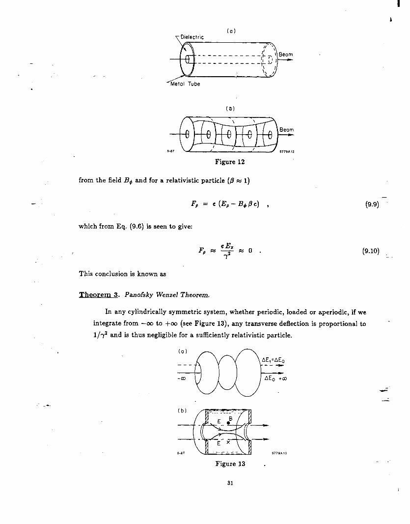
y Dielectric

%etol Tube

(b)

Figure 12

from the field B+ and for a relativistic particle (p k: 1)

- FP = 4Ep-B&) ,

which from Eq. (9.6) is seen to give:

e& Fp w - r2

wo.

(9.9) -

(9.10) I.

This conclusion is known as

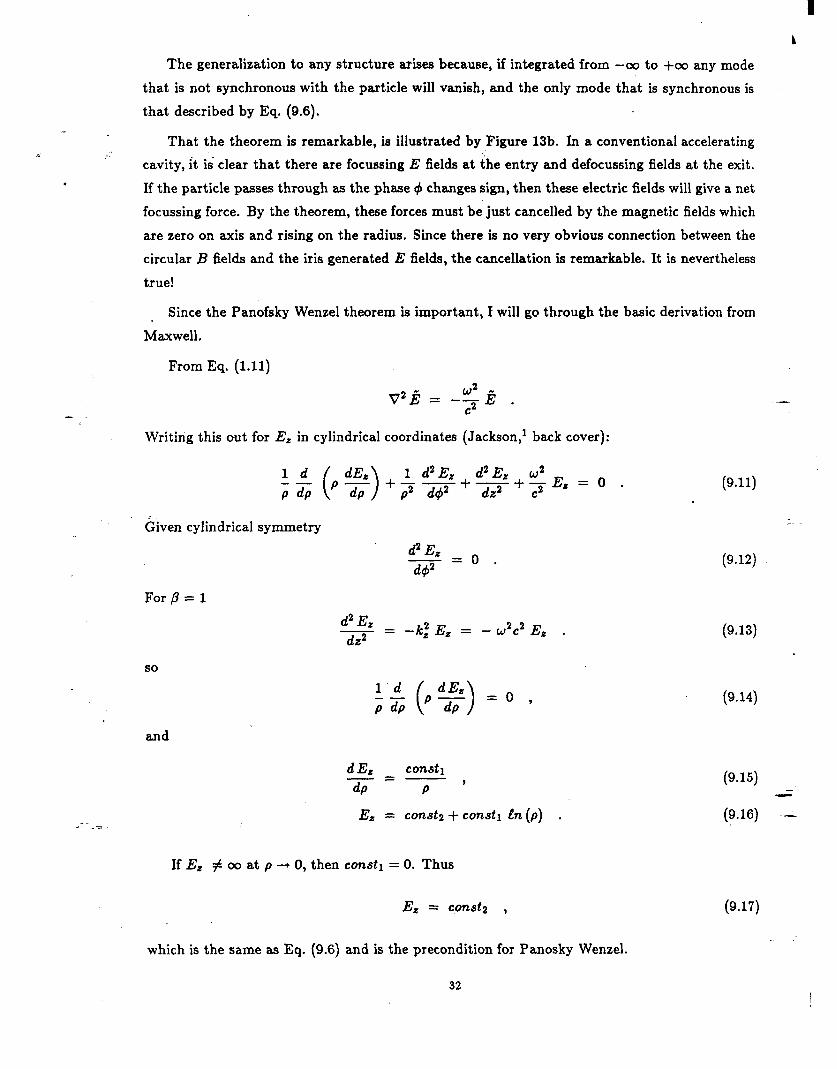
Theorem 3. Panofsky Wenzel Theorem.

In any cylindrically symmetric system, whether periodic, loaded or aperiodic, if we

integrate from -oo to +oo (see Figure 13), any transverse deflection is proportional to

l/r2 and is thus negligible for a sufficiently relativistic particle.

Figure 13 .

31

The generalization to any structure arises because, if integrated from -oo to +oo any mode

that is not synchronous with the particle will vanish, and the only mode that is synchronous is

that described by Eq. (9.6).

.

That the theorem is remarkable, is illustrated by Figure 13b. In a conventional accelerating

cavity, it is clear that there are focussing E fields at the entry and defocussing fields at the exit.

If the particle passes through as the phase 4 changes sign, then these electric fields will give a net

focussing force. By the theorem, these forces must be just cancelled by the magnetic fields which

are zero on axis and rising on the radius. Since there is no very obvious connection between the

circular B fields and the iris generated E fields, the cancellation is remarkable. It is nevertheless

true!

Since the Panofsky Wenzel theorem is important, I will go through the basic derivation from

Maxwell.

From Eq. (1.11)

- Writing this out for Ez in cylindrical coordinates (Jackson,’ back cover):

1 d2Ez d2Ez -- - “zE,=O. + p2 drj2 + t&2 + ~2

&iven cylindrical symmetry

For /3 = 1

d2 Ez ygr= -Cc,2 E, = - w2c2 Ez .

so 1-d -- P dp

and

d& const1 -=- dp P ’

EZ = constz + constl h (p) . (9.16) -2

If Ez # 00 at p 3 0, then con&l = 0. Thus

EL = constz ,

(9.11)

(9.12)

(9.13)

(9.14)

(9.15) -

(9.17)

which is the same as Eq. (9.6) and is the precondition for Panosky Wenzel.

32

Now we go back to Maxwell Eq. (1.7)

v xi? = iwi? .

. Going again to the back cover of Jackson’ and writiig out the azimuthal cylindrical component:

(2-F) = iwB4 . (9.18)

From Eq. (9.17)

d& o -=

dp

,

and for a wave propogating at c

d EP .W - = ik,E, = ;-Ep, dz C

- so

.W iwBg = r;E, .

Now the transverse force on a particle moving at /3 = 1 in the z direction:

Fp = e (Ep - c B,+) ,

which from Eq. (9.19) gives

F,, = 0 .

(9.19)

(9.20)

Wonderful!

33

References

1. J. D. Jackson, Classical Electrodynamics, 2nd Edition, John Wiley & Sons.

2. W. Willis, CERN Report 75-9 (1975).

. 3. T:-T$jima and J. .M. Dawson, Laser Electron A&elerator, Physical Review Letters 43, 267

(1979).

4. C. Joshi et al., Ezperimental Study of Beat Wave Ezcitation of High Phase Velocity Space

Charge Waves in a Plasma for Particle Acceleration, Proc Laser Act. of Particles, Malibu,

CA, p. 99 (1985) and T. Katsouleas et al., Plasma Accelerators, ibid., p. 63 (1985).

5. P. Chen and J, M. Dawson, The Plasma Wake Field Accelerator, ibid., p. 201.

6. R. B. Palmer, Interaction of Relativistic Particles and Free Electromagnetic Waves in the

Presence of a Static Helical Magnet, J. Applied Physics 43, 3014 (1972).

7. C. Pellegrini et al., The Report of the Working Group on Far Field Acceleration, Proc. Laser

Accel. of Particles, Los Alamos, p. 138 (1982). -

8. R. H. Pantell, Electron (and Positron) Acceleration with Lasers, in Laser

Interactions and Related Plasma Phenomena, 6, Plenum Pub. Co., New York (1983),

pp. 1083-1092.

.- 9. R. B. Palmer, A Laser-Driven Grating Linac, Particle Accelerators 11, 81 (1980).

10. J. D. Lawson, Rutherford Lab. Report RL-75-043 (1975); IEEE Transactions on Nuclear

Science, NS-26,4217 (1979).

11. W. K. H. Panofsky and W. A. Wenzel, Rev. Sci. Instrum. 27, 967 (1956).

4

--

34