Panel Data Unit Roots Tests Using Various Estimation Methodsspot.colorado.edu/~mcnownr/working_papers/panel-unit-root-tests.pdf · Panel Data Unit Roots Tests Using Various Estimation

Panel Data Unit Roots Tests Using VariousEstimation Methods

NAM T. HOANG∗and ROBERT F. MCNOWNDepartment of Economics - University of Colorado at Boulder

Abstract

In this paper, the performances of panel data unit root tests are considered andvarious estimation methods under different properties of data are compared. It is shownthat weighted symmetric estimation increases the power of the tests without adverselyaffecting the size, for most data properties and most panels of dimensions N and T.The presence of serial correlation and cross-sectional correlation does not reduce thepower of the tests significantly.

Keywords: Panel unit root; cross-section correlation; serial correlationJEL classification: C12; C15; C22; C23

∗Correspondent author, email: [email protected]

1

mailto:[email protected]

1 Introduction

Since Levin and Lin (1993) established the foundations for panel unit root tests, a few tests

for panel unit roots have been proposed. Among those, the most common tests in practice

are Levin-Lin(LL), Im-Pesaran-Shin (1997)(IPS) and Maddala-Wu (1999)(MW).

Im-Pesaran-Shin (2003) did the Monte-Carlo simulations to compare the test that they

proposed (IPS) and the Levin-Lin test, under the assumption of no cross-sectional correlation

in panels, and they showed that the IPS test is more powerful than the LL test. Maddala-Wu

(1999) also did simulations to compare three tests: LL, IPS and their own test MW. They

generated the data with cross-sectional correlation, and the variance-covariance matrix of

the cross-section error terms was randomly generated. They found the performance of the

LL test to be the worst. Although all three tests exhibit size distortion and low power under

cross-sectional dependence, the MW test generally performs better than the LL and IPS

tests.

O’Connell (1998) was the first author to note that cross-sectional correlation in panel data

will have negative effects on the LL panel unit root test, making the test have substantial size

distortion and low power. In his paper, he did a Monte-Carlo simulation to study the impact

of cross-section correlation on the size and power of the Levin-Lin test and he proposed using

GLS estimators instead of OLS estimators in the Levin-Lin test to increase power.

Kristian (2005) studied the performance of the Levin-Lin test under cross-sectional cor-

relation. In his DGP, he controlled the magnitude of the correlation, and he found results

similar to the results of O’Connell (1998). He also proposed to use the panel corrected

standard error (PCSE) estimator instead of the OLS standard error in the LL test, arguing

that the the PCSE-based test has better size and more power when compared to the LL

test. Strauss (2003) did a Monte-Carlo simulation of the IPS test, and found that the mag-

nitude of the contemporaneous correlation is important in the IPS test, and the demeaning

2

procedure across the panel that Im et al. (2003) suggest doesn’t eliminate this problem.

Of the three popular panel unit roots tests (LL, IPS and MW), the LL test is of limited

use, because the null hypothesis and the alternative hypothesis are so strict that it is not

realistic in practice. A comparison between the IPS or MW test and the LL test is not

valid because the alternative hypotheses of these tests are different. The MW and IPS tests

are more directly comparable. The intent of my paper is to perform such a comparison

employing both least squares and weighted symmetric estimators.

Comparing the IPS and MW tests in the Maddala and Wu paper (1999), the data gen-

erating process is constructed with both serial correlation and contemporaneous correlation,

but the serial correlation coefficients are randomly generated and the variance-covariance

matrix of contemporaneous errors is also a random positive definite matrix. In this paper,

we examine the performance of the IPS and MW tests with different estimation methods

under alternative data generating processes. We construct separate DGPs, varying the mag-

nitude of the correlation between cross-sections, to study the impact of serial correlation

and contemporaneous correlation separately. In addition, it is well known that a moving-

average component in the series will cause size distortion and lower power of unit roots tests.

We take this into account to examine the performance of the IPS and MW tests under the

moving-average component DGP.

Despite the fact that the IPS and MW test can be performed with any unit-root test

(for a single time series in each cross-section), it has been only used with the Dickey-Fuller

(DF) or Augmented Dickey-Fuller (ADF) estimation equations until now. We know that

although often used, the ADF test (as well the Phillips-Perrons (PP) test) has substantial

size distortion and lack of power in some environments. Maddala and Kim (2002) surveyed

unit root tests other than the ADF and PP tests, including a weighted symmetric(WS)

estimator test. Quoting Maddala and Kim: ”..it is better to use one of these than the ADF

and PP tests discussed in previous chapter. It is time now to completely discard the ADF

3

and PP test (they are still used often in applied work!)”(p.145). For this reason, we use both

least squares and the weighted symmetric estimation approach with the IPS and MW test,

examining their performance under different data properties. The simulation results show

that the panel unit root tests with WS estimation have more power with reasonable size

properties compared with the tests using DF and ADF estimation in general.

2 Panel data unit roots tests

2.1 The Im-Pesaran-Shin Test

The model is:

yi,t = αi + ρiyi,t−1 + εi,t (1)

t = 1, 2, . . . , T

The null and alternative hypotheses are defined as:

H0 : ρi = 1, i = 1, 2, . . . , N (2)

against the alternatives

HA : ρi < 1, i = 1, 2, . . . , N1; ρi = 1, i = N1 + 1, N1 + 2, . . . , N (3)

They use separate unit root tests for the N cross-section units. The DF regression:


t = 1, 2, . . . , T

4

or ADF regression:

yi,t = αi + ρiyi,t−1 +

pi∑j=1

θij∆yi,t−j + εi,t (5)

t = 1, 2, . . . , T

is estimated and the t-statistic for testing ρi = 1 is computed. Let ti,T (i = 1, 2, . . . , N)

denote the t-statistic for testing unit roots in individual series i, and let E(ti,T ) = µ and

V (ti,T ) = σ2. Then

tN,T =1

N

N∑i=1

ti,T (6)

and√

N(tN,T − µ)

σ

N=⇒ N(0, 1)

The IPS test is a way of combining the evidence on the unit root hypothesis from N unit

root tests performed on N cross-section units. The test assumption is that T is the same for

all cross-section units and hence E(ti,T ) and V (ti,T ) are the same for all i, so the IPS test

is applied only for balanced panel data. In the case of serial correlation, IPS propose using

the ADF t-test for individual series. E(ti,T ) and V (ti,T ) will vary as the lag length included

in the ADF regression varies. They tabulated E(ti,T ) and V (ti,T ) for different lag lengths.

In practice, to use their tables one is restricted to using the same lag length for all the ADF

regressions for individual series.

In principle, the IPS test also can be used in association with any parametric unit-root

test, as long as the panel is balanced and all the t-statistcs for the unit-root in every cross-

section are identically distributed so that they will have the same variance and mean. Then

the Central Limit Theorem(CLT) can be applied. Although the IPS test requires a balanced

panel, it is the test most often used in practice because it is simple and easy to use. Until

now, people have only used IPS with the ADF or DF estimation equation. We apply the

5

IPS test using weighted symmetric estimation. To do this, we estimate by simulation the

variances and means of the weighted symmetric t-statistic with different values of T and lag

lengths of the ADF equation, and then use these variances and means to compute the test

statistics which have the standard normal distribution under the CLT.

2.2 Maddala and Wu Test

Maddala and Wu (1999) proposed the use of the Fisher (pλ) test which is based on com-

bining the p-values of the test-statistic for a unit root in each cross-sectional unit. Let πi

be the p-value from the ith-test such that πi are U [0, 1] and independent, and −2logeπi has

a χ2 distribution with 2 degrees of freedom. So pλ = −2∑N

i=1 logeπi has a χ2 distribution

with 2N degrees of freedom. The null and alternative hypotheses are the same as in the

IPS test. Applying the ADF estimation equation in each cross-section, we can compute the

ADF t-statistic for each individual series, find the corresponding p-value from the empiri-

cal distribution of ADF t-statistic (obtained by Monte-Carlo simulation), and compute the

Fisher-test statistics and compare it with the appropriate χ2 critical value.

The test proposed by Maddala-Wu (1999) using Fisher’s test is promising, for the following

two reasons: First, it can be performed with any unit root test on a single time-series. It

should be kept in mind that the MW test does not require using the same unit-root test in

each cross section (in practice, one usually uses the same unit root test in each cross-section).

Second, it does not require a balanced panel as the IPS test does, so T can differ over cross-

sections. The main disadvantage of the MW test is that the p-values for each t-statistic in

a cross-section have to be derived by Monte-Carlo simulation. Because of this, IPS may be

favored over MW, but with more and more powerful computer software available using the

MW test is less of problem.

We also apply the weighted symmetric estimation in the context of MW test, and study

its performance under various data properties. Simulations are conducted to estimate the

6

empirical weighted symmetric distribution of tws with different values of T .

3 Weighted Symmetric Estimation

3.1 Weighted Symmetric Estimation for AR(1) model

Consider the process:

Yt = α + ρYt−1 + εt (7)

t = 2, 3, . . . , T ; εt ∼ N(0, σ2)

The idea of the symmetric estimator is that if a stationary process satisfies this equation,

then it also satisfies the equation:

Yt = α + ρYt+1 + ut (8)

t = 1, 2, . . . , (T − 1); ut ∼ N(0, σ2)

Consider an estimator of ρ that minimizes:

Qw(ρ) =T∑

t=2

wt(yt − ρyt−1)2 +

T−1∑t=1

(1− wt+1)(yt − ρyt+1)2 (9)

where wt , t=2,3,...,T are weights, yt = Yt− y and y = T−1∑T

j=1 yj. The estimator obtained

by setting wt = T−1(t− 1) is called the weighted symmetric (WS) estimator.

The weighted symmetric estimator of ρ is:

ρws =

∑Tt=2 ytyt−1∑T−1

t=2 y2t + T−1

∑Tt=1 y2

t

(10)

7

and the corresponding t-statistic is:

tws = σ−1ws (ρws − 1)(

T−1∑t=2

y2t + T−1

T∑t=1

y2t )

1/2 (11)

Where σ2ws = (T − 2)−1Qw(ρws). Park and Fuller (1995) derived the limiting distribution of

WS t-statistics:

tws =⇒

[∫ 1

0

W (r)2dr −[∫ 1

0

W (r)dr

]2]−1/2

×

×

[W (1)2 − 1

2−W (1)

∫ 1

0

W (r)2dr −∫ 1

0

W (r)2dr + 2

[∫ 1

0

W (r)dr

]2]

Where W (r) is a standard Wiener process on [0,1].

3.2 Weighted Symmetric Estimation for AR(p) model

Consider the pth order autoregressive time series:

Yt = α0 +

p∑i=1

αiYt−i + ei (12)

t = p + 1, . . . , T

where {et}∞t=1 is a sequence of normal independent (0, σ2) random variables. The character-

istic equation associated with (12) is:

mp −p∑

i=1

αimp−i = 0 (13)

8

Assume that |λi| < 1, where λ1, λ2, ..., λp are the roots of the characteristic equation (13). A

stationary time series satisfying (12) also satisfies:

Yt = α0 +

p∑i=1

αiYt+i + ui (14)

t = 1, 2, . . . , T − p

where {ut} ∼ N(0, σ2). We consider a class of estimators of α, obtained by minimizing:

Q =T∑

t=p+1

wt

[Yt − α0 −

p∑i=1

αiYt−i

]2

+

T−p∑t=1

(1− wt+1)

[Yt − α0 −

p∑i=1

αiYt+i

]2

(15)

where wt, t = 1, 2, ..., T are weights and 0 ≤ wt ≤ 1. If wt = 1 in (15) we have the ordinary

least squares estimator. The estimator that minimizes (15) with wt = 0.5 is called the simple

symmetric least squares estimator. The value of α that minimizes (15) with:

wt =

0 t = 1, 2, ..., p

(T − 2p + 2)−1(t− p) t = p + 1, p + 2, ..., T − p + 1

1 t = T − p + 2, T − p + 3, ..., T

(16)

is called the weighed symmetric estimator and is denoted αw. The estimator αw is closely

related to the estimator obtained by maximizing the normal stationary likelihood (Park and

Fuller, 1995). By minimizing Q, we can see the idea of weighted symmetric estimator is that

we use information of weighted observations based on the time lag and lead of the series:

the further the lag of an observation, the smaller is the weighted and the further the lead of

an observation, the smaller is the weighted.

9

Equation (15) can be reparameterized as :

Q =T∑

t=p+1

wt

[Yt − θ0 − θ1Yt−1 −

p∑i=2

θi∆Yt−i+1

]2

+

T−p∑t=1

(1−wt+1)

[Yt − θ0 − θ1Yt+1 −

p∑i=2

θi(−∆Yt+i)

]2

(17)

Where ∆Yt = Yt − Yt−1.

Pivotal t-statistics for the unit root hypothesis θ1 = 1 are constructed by analogy to the

pivotal t-statistics for the usual regression analysis:

tws = [V (θ1)]1/2(θ1 − 1) (18)

where V (θ1) is the estimated variance of the estimated coefficient of Yt−1 in (17). As in the

case of the AR(1) model, Park and Fuller (1995) showed that the limiting distribution of tws

is:

tws =⇒

[∫ 1

0

W (r)2dr −[∫ 1

0

W (r)dr

]2]−1/2

×

×

[W (1)2 − 1

2−W (1)

∫ 1

0

W (r)2dr −∫ 1

0

W (r)2dr + 2

[∫ 1

0

W (r)dr

]2]

Where W (r) is a standard Wiener process on [0,1].

4 Monte-Carlo Investigation Design

4.1 Testing Procedures

The IPS-DF test

The regression equation for each cross-section i:


10

t = 2, 3, . . . , T

is estimated for each cross-section i, i = 1, 2, . . . , N , to calculate the t-statistic for ρi denoted

by ti,T . The table of E(ti,T ) and V (ti,T ) from Im et al. (2003, p.60) gives µ and σ2 for each

T . The panel t-statistic is calculated as:

tDF−N,T =√

N(tDF − µ)

σ

N=⇒ N(0, 1) (20)

where

tDF =1

N

N∑i=1

ti,T (21)

The standard normal critical values are used to study size and power of the test.

The IPS-ADF test

The regression equation for each cross-section i:


p∑j=1


t = p + 1, . . . , T

Here, to choose the appropriate lag length, we employed the rule suggested by Schwert

(1989): p = Int[c(T/100)1/d] with c=4, d=4.

The steps are similar to the IPS-DF test described above: calculate the t-statistic for ρi,

denoted by ti,T , then use the table for E(ti,T ) and V (ti,T ) available in Im et al. (2003, p.66)

to get µ and σ2 for each p and T . The panel t-statistic are calculated as:

tADF−N,T =√

N(tADF − µ)

σ

N=⇒ N(0, 1) (23)

11

where

tADF =1

N

N∑i=1

ti,T (24)

The standard normal critical values are used to study size and power of the test.

The IPS-WS(1) test

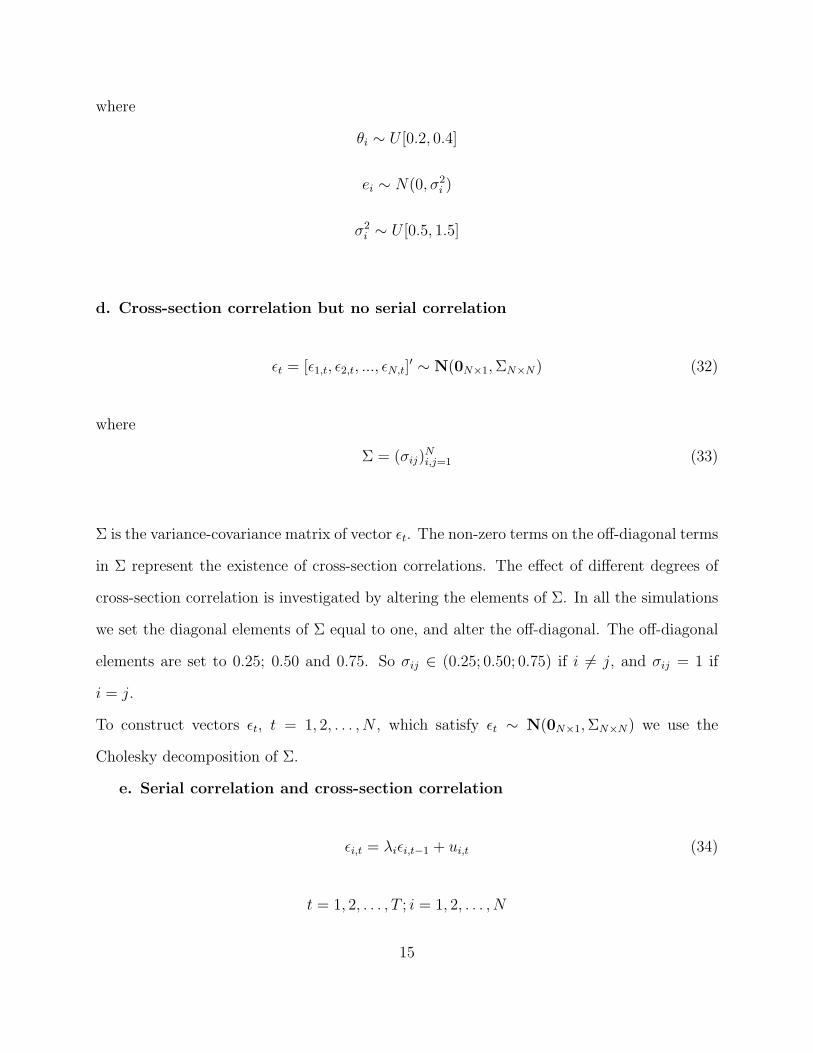
To apply WS estimation in the IPS test, we need to compute means and variances of t-

statistic for the AR(1) model with different values of T. Table 1 gives the moments of

t-statistic of the weighted symmetric estimator for the AR(1) model based on 200,000 sim-

ulations, using the formula:


T−1∑t=2

y2t + T−1

T∑t=1

y2t )

1/2 (25)

where σ2ws = (T − 2)−1Qw(ρws). Then WS estimation is used to compute the tws for each

cross-section, follow by the steps of Im et al. (2003) as in the IPS-DF test previously

described.

The IPS-WS(p) test

Table 2 shows the moments of t-statistics of the weighted symmetric estimator, for the AR(p)

model with lags of number p and T. The lag p is calculated by p = Int[4(T/100)1/4]. In

each cross-section we estimate θj which minimize (17). From these estimates, compute the

t-statistic for the hypothesis θ1 = 1 for each cross-section of the panel, and then follow the

remaining IPS test procedures.

The MW-ADF test

The ADF equation for each individual series, with the lag length p = Int[4(T/100)1/4], is

estimated:


p∑j=1


t = 1, 2 . . . , T

12

The MW test requires deriving the distribution of the Dickey-Fuller t-statistic, for which

50,000 simulations were generated for different T and p. Then the p-values πi for each

ADF t-statistic could be derived. Consequently, the MW-ADF statistic pλ is calculated as:

pλ = −2∑N

i=1 logeπi ∼ χ22N . For the critical values of MW-ADF statistics pλ for each N, we

use the χ2 table.

The MW-WS test

For this test, the WS estimation was applied for each individual series. For the WS(1) model,

the t-statistic were computed by:


T−1∑t=2

y2t + T−1

T∑t=1

y2t )

1/2 (27)

For the WS(p) model, the estimation involves minimization of (17), from which the t-statistic

for testing the hypothesis θ1 = 1 was computed. 50,000 simulations were generated to get

the empirical WS distribution of tws for different values of p and T. Then based on the WS

empirical distribution of tws, the p-values πi of each t-statistic in each cross-section can be

derived. After that MW test procedure is followed.

4.2 Data Generation Processes

The basic DGP is:

yi,t = (1− ρ)αi + ρyi,t−1 + εi,t (28)

t = 1, 2, . . . , T ; i = 1, 2, . . . , N

where

αi ∼ U [0, 1]

13

ρ =

1 for size

0.9 for power(29)

We set yi,0 = 0. To reduce the influence of the initial condition we generated T+50 time

series observations for each cross-section, then eliminated the first 50 observations and used

only the last T time series observation for each cross-section. The parameter values adopted

here are based on the values used in the Im et al. (2003) and the Maddala and Wu (1999)

papers. We consider five distinct sets of DGP as following:

a. No serial correlation and no cross-section correlation

εi,t ∼ N(0, σ2i ) and σ2

i ∼ U [0.5, 1.5] ; t = 1, 2, . . . , T ; i = 1, 2, . . . , N

b. Serial correlation but no cross-section correlation

εi,t = λiεi,t−1 + ui,t (30)

t = 1, 2, . . . , T ; i = 1, 2, . . . , N

where

λi ∼ U [0.2, 0.4]

ui,t ∼ N(0, σ2i )

σ2i ∼ U [0.5, 1.5]

c. Moving-average serial correlation

εi,t = ei,t − θiei,t−1 (31)

t = 1, 2, . . . , T ; i = 1, 2, . . . , N

14

where

θi ∼ U [0.2, 0.4]

ei ∼ N(0, σ2i )

σ2i ∼ U [0.5, 1.5]

d. Cross-section correlation but no serial correlation

εt = [ε1,t, ε2,t, ..., εN,t]′ ∼ N(0N×1, ΣN×N) (32)

where

Σ = (σij)Ni,j=1 (33)

Σ is the variance-covariance matrix of vector εt. The non-zero terms on the off-diagonal terms

in Σ represent the existence of cross-section correlations. The effect of different degrees of

cross-section correlation is investigated by altering the elements of Σ. In all the simulations

we set the diagonal elements of Σ equal to one, and alter the off-diagonal. The off-diagonal

elements are set to 0.25; 0.50 and 0.75. So σij ∈ (0.25; 0.50; 0.75) if i 6= j, and σij = 1 if

i = j.

To construct vectors εt, t = 1, 2, . . . , N , which satisfy εt ∼ N(0N×1, ΣN×N) we use the

Cholesky decomposition of Σ.

e. Serial correlation and cross-section correlation

εi,t = λiεi,t−1 + ui,t (34)

t = 1, 2, . . . , T ; i = 1, 2, . . . , N

15

where

λi ∼ U [0.2, 0.4]

and

ut = [u1,t, u2,t, ..., uN,t]′ ∼ N(0N×1, ΣN×N) (35)

with σij = 0.5 if i 6= j, and σij = 1 if i = j.

5 Size and Power of Tests

The results of the simulation experiments are reported in Tables 3-7. In all cases, 3000 trials

are used to examine the size and power properties.

Table 31 presents the first set of experiments when there is no serial correlation in indi-

vidual series and no cross-section correlation between series. The critical value of the 5%

significance level is used to calculate the size and power of the tests. For all five tests , the

size is close to 5% of the nominal size, and the size does not change much when N and T

are increased. In every case, the empirical size lies between 0.04 and 0.06. In this table the

IPS-ADF and MW-ADF tests are over-parameterized, which adversely affects their power,

but not the size. We can see that the power of the tests vary, but for every combination of

N and T, the IPS-WS(1) test has the most power. The second most powerful test is the

MW-WS(1) test. Compared to the IPS-DF, the IPS-ADF and MW-ADF are less powerful

because of their over-parameterization. When the number of cross-sections N or number

of observations T increases, the power of all five tests increase. Power increases faster with

T than with N so that cases with large N (50) and small T (10) show low power overall.

The power varies more across the tests when N and T are small, so that with N = 10 and

T = 25, the power of the IPS-WS(1) test is 56%, compared with 40% for the MW-WS(1),

1All simulations are performed by using Matlab 7.0 on a 3.44 GHz, 2GB Ram PC. The programs areavailable upon requested.

16

28% for the IPS-DF and only 16% for the MW-ADF. The IPS-WS(1) seems to be the best

choice in the case of no serial correlation and no cross-sectional correlation but if the panel

is unbalanced, the MW-WS(1) test may be preferred.

Table 4 summarizes the size and power of tests in the case when there is serial correlation

but no cross-sectional correlation. The IPS-DF test has strong size distortion towards zero,

which worsens when N and T increase. The reason is the under-parameterization of the DF

estimation equation in a series which is serially correlated. The IPS-ADF and MW-ADF

tests remain almost as good for size as in Table 3 but are somewhat over sized for small T .

The size of IPS-WS(p) and MW-WS(p) tests are still close to the nominal 5%, but are a

little under sized with small T . The greatest size distortion for all tests is when T is small,

and it increases when N increases, but when T increases as well, the size becomes acceptable

again. Size distortion is not severe in this table for all tests except the IPS-DF test. The

IPS-WS(p) test is a little deficient in size, but it tends to reduce the probability of a type I

error in testing a hypothesis.

For the power of the tests, we see that the IPS-WS(p) test consistently has the the best

power, and the power of the MW-WS(p) test is the second highest. The IPS-DF test is

very weak in power especially when T is small, so this test should not be used in the case

of serial correlation. When T and N are small, the WS(p) estimation brings more power to

the tests as compared with the ADF estimation. When T = 100 and N ≥ 25 all of the tests’

power tends to 1. They are different when T ≤ 50. The IPS-WS(p) test should be chosen in

this case, unless the panel is unbalanced, in which case the MW-WS(p) test should be used.

Power rises more strongly with increases in T, compared with increases in N. Power is low

for T = 10, even when N = 50.

Table 5 reports the size and power of the tests when there is a moving-average component

in the errors of each individual series. The IPS-DF test has a very serious size distortion,

which grows quickly when T is increasing. The other four tests show some size distortion,

17

tending to be a little above the nominal 5% size in some cases. The IPS-WS(p) and MW-

WS(p) tests have slightly more distortion compared with the IPS-ADF and MW-ADF tests.

When N = 50, T = 10 and T = 25, they have the most distortions, which are 0.148, 0.143

for IPS-WS(p) and 0.105, 0.136 for MW-WS(p). The IPS-ADF and the MW-ADF show

least size distortion. WS tests show greatest distortion when N is large and T is small.

For the power of the test, the IPS-DF test power looks good, but this test can not be

used because it has a serious size distortion with probabilities of a type I error near one. Of

all four remaining tests, the IPS-WS(p) test has the strongest power for every value of N

and T , followed by the MW-WS(p), IPS-ADF and the MW-ADF test. With the small trade

off in size distortion (allowing greater risk of type I error) one may use the IPS-WS(p) or

MW-WS(p) test to have a higher power, which reduces a probability of committing a type

II error. To avoid type I error, the MW-ADF or IPS-ADF tests may be preferred in this

case, although power is much lower.

Table 6A reports the size and power of the tests when there is a cross-sectional correlation

coefficient of [σ = 0.25] and no serial correlation. In this case, O’Connell (1998) found that

the size of the Levin-Lin test is distorted upwards. In contrast to this, all five tests presented

here have sizes distorted downwards with all sizes close to zero, especially the IPS-WS(p)

and MW-WS(p) tests. This shows that the normal distribution locus of the IPS-WS(p) test

shifts to the right, and the chi-squared distribution locus of the MW-WS(p) test shifts to the

left. With all sizes close to zero, the probability of a type I error is lower. It is interesting

that the power of all the tests seems not to be affected much compared with the results in

Table 3 (under no serial and cross-sectional correlation). The order from the most powerful

to the least powerful of tests is the same as in Table 3, which is: IPS-WS(p), MW-WS(p),

IPS-DF, IPS-ADF and MW-ADF. The tests’ power in this table are a little less than those

in Table 3. The reason for this may be because of the over-parameterization in ADF and

WS(p) estimations. It is also of note here that the over-parameterization is less serious

18

than the under-parameterization problem. In this case the IPS-DF may be preferred to test

the hypothesis of a unit- root, because it has the best size and relatively good power when

T ≥ 25.

Table 6B shows the results of the experiment that is the same as in Table 6A, except

the cross-section correlation coefficient now is [σ = 0.5]. The size now is slightly higher in

all three tests using DF or ADF estimations. It tends to exceed the 5% nominal size when

T=10, and it drops below 5% when T increases. The power of all the tests are slightly

higher than those in Table 6A when T is small and get smaller than those in Table 6A when

N and T increase. We see that when σ is larger, all of the tests’ powers are better for small

values of T, and a bit less power for larger T. The power of the IPS-WS(p) and MW-WS(p)

tests still dominate the other three tests for almost every value of N and T.

In Table 6C, the cross-section correlation coefficient is chosen as [σ = 0.75]. As we see in

the table, most of the sizes are higher than those in Table 6B. All tests using DF and ADF

estimations have greater than 5% size when T=10 but their size drops to 5% and lower when

T increases. The size of IPS-WS(p) and MW-WS(p) tests is slightly increased but they are

still very close to zero for all value of N and T. The power of tests are better than those in

Table 6A when N ≤ 10 and T ≤ 25, but they slightly decrease when N and T are larger.

The power of the IPS-WS(p) test still dominates for all cases of N and T.

Combining tables 6A, 6B and 6C, we see that when the magnitude of the cross-section

correlation coefficient increases, the size of all three tests using DF or ADF estimation

becomes larger. Especially when N=10, the power of the tests gets stronger for small T

and getting weaker for large T as cross-sectional correlation is increasing. The size of the

two tests using WS(p) estimation are close to zero, which means the locus of these tests’

distributions shifts away from a standard position (to the right for IPS-WS test, and to the

left for MW-WS test). In the case when there is cross-sectional correlation and no serial

correlation in the panel, and when N ≥ 10 and T ≥ 50, the IPS-DF test may be a better

19

choice, as it has both good size and power. When T or N is small, we can use the IPS-WS(p)

test with a balanced panel or the MW-WS(p) test with an unbalanced panel to get more

power in testing the hypothesis of nonstationarity in the panel.

The last set of experiments is shown in Table 7, where in the DGP, both serial correlation

and cross-sectional correlation are allowed, with the cross-sectional correlation coefficient set

to [σ = 0.5]. Compared to the results in the case of Table 6B, adding serial correlation

seriously affects the performance of the IPS-DF test, but it does not affect the performances

of the other four tests very much. The size of the IPS-DF test is closer to 0.05 than those

in Table 4, even though DF estimation is also under-parameterized in this case. It may

be because the presence of cross-sectional correlation remedies the size distortion of DF

estimation, but the power of the IPS-DF test drops dramatically. The other four tests IPS-

ADF, IPS-WS(p), MW-ADF and MW-WS(p) perform pretty much the same as they do

in the case of Table 6B, which is without serial correlation. We can see here that over-

parameterization in Table 6B does not impact the size and power of the tests very much

compared with the correct-parameterization in the case of Table 7. The IPS-WS(p) test is

the most powerful, followed by the MW-WS(p) in every case of N and T.

For all tests using ADF or WS(p) estimation, serial correlation in individual series is not

a serious problem. The presence of cross-sectional correlation affects all tests. It usually

lowers the size of tests when T increases, but it does not change the power of the tests very

much compared with the case with no cross-sectional correlation.

6 Conclusions

In this paper, we consider the use of weighted symmetric estimation in the context of sta-

tionary testing in panel data. The Monte-Carlo simulations are made to investigate the

performance of the IPS and MW unit root tests in panels without time trend under differ-

20

ent data properties. The of moments of t-statistic for weighted symmetric estimators are

computed for use with the IPS test. The weighted symmetric estimation is compared to DF

and ADF estimation, two commonly used estimation methods. We found that in the case

of panel data without cross-sectional correlation, tests using weighted symmetric estimation

dominate those using the DF and ADF estimation in terms of power of the test, regardless

of whether there is serial correlation in each series or not. Tests using weighted symmetric

estimation also have the best power when there is a moving-average in the errors. When

there is cross-sectional correlation between individual series, in most cases the size of tests

using weighted symmetric estimation is zero, which reduces a probability to commit a type

I error in testing hypotheses, and the power of tests using weighted symmetric estimation is

still better than those using DF or ADF estimation. Across all environments there appear

to be strong gains in powers afforded by use of the weighted symmetric procedure in panel

unit root tests.

21

REFERENCES

Breuer, McNown R, and Wallace M (2002) ”Series-specific Unit Root tests with Panel

Data”, Oxford Bullertin of Economics and Statistics, 64(5), 527-545

Fuller W.A (1996) ”Introduction to Statistical Time Series”, second edition. John Wiley

& Sons, Inc. New York

Kristian Jonsson(2005)”Cross-sectional Dependency and Size Distortion in a Small-sample

Homogeneous Panel Data Unit Root Test”, Oxford Bulletin of Economics and Statistics 67

Im K.S, Pesaran M.H, and Shin Y (2003) ”Testing for Unit Roots in Heterogeneous

Panels”, Journal of Econometrics 115 (revise version of 1997’s work), 53-74

Levin A, Lin C.F, Chu C.J (2002) ”Unit root tests in panel data: asymptotic and finite-

sample properties” Journal of Econometrics 108 (revise version of 1992’s work),1-24

Maddala G.S and Kim (2002) ”Unit Roots, Cointegration and Structure Change”, Cam-

bridge University Press

Maddala G.S and Shaowen Wu (1999)”A comparative study of unit root tests with panel

data and new simple test”, Oxford Bullertin of Economics and Statistics, Speccial issue,

631-652

O’Connell (1998) ”The overvaluation of purchasing power parity”, Journal of Interna-

tional Economics 44, 1-19.

Pantula S.G, Gonzalez-Farias G and Fuller W.A (1994) ”A comparison of unit-root test

criteria”, Journal of Business and Economic Statistics 12, 449-459

Park H.J and Fuller W.A (1995) ”Alternative estimators and unit root test for the au-

toregressive process”, Journal of Time Series Analysis 16, 415-429

Schwert G.W (1989) ”Tests for Unit Roots: A Monte Carlo Investigation”, Journal of

Business and Economic Statistics 7, 147-159

Strauss J and Yigit T (2003) ”Shortfall of panel unit root testing ”, Economics Letter 81,

309-313

22

TABLE 1: Moments of t-statistics of the weighted symmetricestimator for the AR(1 ) model

T MEAN VARIANCE5 -1.4541 1.19486 -1.3996 1.01207 -1.3619 0.95118 -1.3349 0.91709 -1.3118 0.877710 -1.2962 0.863815 -1.2460 0.818220 -1.2092 0.797025 -1.2104 0.792730 -1.2002 0.793540 -1.1884 0.782050 -1.1817 0.774160 -1.1753 0.775870 -1.1758 0.772780 -1.1642 0.769390 -1.1680 0.7715100 -1.1665 0.7726150 -1.1614 0.7684200 -1.1599 0.7681500 -1.1571 0.76811000 -1.1575 0.7660NOTES: means and variances in this table are computed by stochastic simulationswith 200,000 replications. The underlying data is generated by yt = yt−1 + εt,where εt ∼ N(0, σ2) with σ2 ∼ U [0.5, 1.5]. T+50 observations are generated andthe first 50 observations are eliminated, using only the last T observations.

23

TABLE 2: Moments of t-statistics of the weighted symmetricestimator for the AR(p) model

p T MEAN VARIANCE2 7 -0.7209 1.00782 8 -0.7520 1.03312 9 -0.7734 1.03692 10 -0.7932 1.05312 15 -0.8708 1.07022 20 -0.9235 1.06112 25 -0.9608 1.04422 30 -0.9873 1.03163 40 -1.0078 1.00673 50 -1.0319 0.99573 60 -1.0483 0.97783 70 -1.0605 0.97043 80 -1.0765 0.95503 90 -1.0814 0.95454 100 -1.0604 0.95664 150 -1.0894 0.93194 200 -1.1022 0.9162NOTES: means and variances in this table are computed by stochastic simulationswith 200,000 replications. The underlying data is generated by yt = yt−1 + εt,where εt ∼ N(0, σ2) with σ2 ∼ U [0.5, 1.5]. T+50 observations are generated andthe first 50 observations are eliminated, using only the last T observations. p isdecided by p = Int[c(T/100)1/d] with c=4, d=4.

24

TABLE 3: Size and power of panel unit root tests withno serial correlation and no cross-sectional correlation

N T IPS-DF IPS-ADF IPS-WS(1) MW-ADF MW-WS(1)SIZE

5 10 0.048 0.048 0.054 0.046 0.04925 0.051 0.045 0.050 0.044 0.05150 0.046 0.043 0.047 0.046 0.050100 0.049 0.046 0.054 0.054 0.053

10 10 0.057 0.059 0.053 0.053 0.05025 0.047 0.052 0.052 0.054 0.04750 0.043 0.042 0.043 0.046 0.047100 0.045 0.045 0.048 0.051 0.048

25 10 0.054 0.046 0.058 0.044 0.05625 0.045 0.048 0.050 0.046 0.05750 0.042 0.044 0.048 0.044 0.051100 0.044 0.041 0.045 0.050 0.046

50 10 0.060 0.055 0.050 0.053 0.05125 0.058 0.054 0.051 0.049 0.04450 0.048 0.043 0.047 0.046 0.053100 0.052 0.050 0.057 0.055 0.052

POWER5 10 0.073 0.064 0.103 0.058 0.088

25 0.169 0.126 0.320 0.107 0.24350 0.459 0.318 0.787 0.243 0.661100 0.969 0.857 1.000 0.762 0.996

10 10 0.093 0.083 0.156 0.071 0.12625 0.279 0.214 0.563 0.158 0.40750 0.777 0.604 0.982 0.439 0.924100 1.000 0.994 1.000 0.967 1.000

25 10 0.143 0.126 0.290 0.095 0.21225 0.565 0.450 0.924 0.260 0.75950 0.991 0.943 1.000 0.787 1.000100 1.000 1.000 1.000 1.000 1.000

50 10 0.221 0.188 0.483 0.114 0.34325 0.825 0.712 0.998 0.434 0.96050 1.000 0.999 1.000 0.972 1.000100 1.000 1.000 1.000 1.000 1.000

NOTES: This table reports the size and power of the tests. The underlying data is generatedby yi,t = (1− ρ)αi + ρyi,t−1 + εi,t, where αi ∼ U [0, 1] and εit ∼ N(0, σ2

i ) with σ2i ∼ U [0.5, 1.5] .

αi and σ2i are generated once and fixed in all replications, there is no serial correlation and no

cross-sectional correlation. ρ = 1 for size and ρ = 0.9 for power. WS(1) denotes the weightedsymmetric estimation for AR(1) model. T+50 observations are generated and the first 50observations are eliminated, using only last T observations. Number of replications is set to3,000 for computing the empirical size and power of all five tests. The size and power of testsare computed at the 5% nominal level.

25

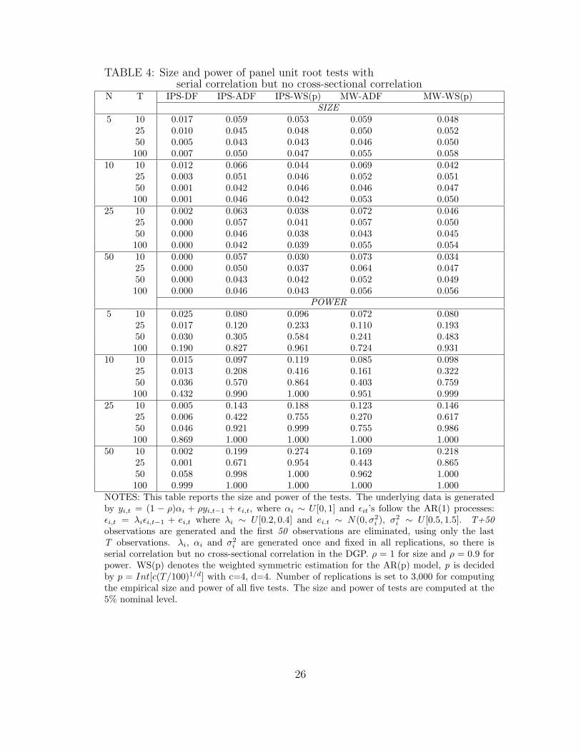
TABLE 4: Size and power of panel unit root tests withserial correlation but no cross-sectional correlation

N T IPS-DF IPS-ADF IPS-WS(p) MW-ADF MW-WS(p)SIZE

5 10 0.017 0.059 0.053 0.059 0.04825 0.010 0.045 0.048 0.050 0.05250 0.005 0.043 0.043 0.046 0.050100 0.007 0.050 0.047 0.055 0.058

10 10 0.012 0.066 0.044 0.069 0.04225 0.003 0.051 0.046 0.052 0.05150 0.001 0.042 0.046 0.046 0.047100 0.001 0.046 0.042 0.053 0.050

25 10 0.002 0.063 0.038 0.072 0.04625 0.000 0.057 0.041 0.057 0.05050 0.000 0.046 0.038 0.043 0.045100 0.000 0.042 0.039 0.055 0.054

50 10 0.000 0.057 0.030 0.073 0.03425 0.000 0.050 0.037 0.064 0.04750 0.000 0.043 0.042 0.052 0.049100 0.000 0.046 0.043 0.056 0.056

POWER5 10 0.025 0.080 0.096 0.072 0.080

25 0.017 0.120 0.233 0.110 0.19350 0.030 0.305 0.584 0.241 0.483100 0.190 0.827 0.961 0.724 0.931

10 10 0.015 0.097 0.119 0.085 0.09825 0.013 0.208 0.416 0.161 0.32250 0.036 0.570 0.864 0.403 0.759100 0.432 0.990 1.000 0.951 0.999

25 10 0.005 0.143 0.188 0.123 0.14625 0.006 0.422 0.755 0.270 0.61750 0.046 0.921 0.999 0.755 0.986100 0.869 1.000 1.000 1.000 1.000

50 10 0.002 0.199 0.274 0.169 0.21825 0.001 0.671 0.954 0.443 0.86550 0.058 0.998 1.000 0.962 1.000100 0.999 1.000 1.000 1.000 1.000

NOTES: This table reports the size and power of the tests. The underlying data is generatedby yi,t = (1 − ρ)αi + ρyi,t−1 + εi,t, where αi ∼ U [0, 1] and εit’s follow the AR(1) processes:εi,t = λiεi,t−1 + ei,t where λi ∼ U [0.2, 0.4] and ei.t ∼ N(0, σ2

i ), σ2i ∼ U [0.5, 1.5]. T+50

observations are generated and the first 50 observations are eliminated, using only the lastT observations. λi, αi and σ2

i are generated once and fixed in all replications, so there isserial correlation but no cross-sectional correlation in the DGP. ρ = 1 for size and ρ = 0.9 forpower. WS(p) denotes the weighted symmetric estimation for the AR(p) model, p is decidedby p = Int[c(T/100)1/d] with c=4, d=4. Number of replications is set to 3,000 for computingthe empirical size and power of all five tests. The size and power of tests are computed at the5% nominal level.

26

TABLE 5: Size and power of panel unit root tests witha moving-average component in errors


5 10 0.282 0.053 0.076 0.047 0.06425 0.496 0.062 0.071 0.056 0.07550 0.489 0.044 0.051 0.047 0.055100 0.629 0.052 0.052 0.055 0.059

10 10 0.432 0.055 0.083 0.044 0.06325 0.653 0.062 0.076 0.059 0.07250 0.803 0.054 0.067 0.056 0.064100 0.847 0.052 0.053 0.055 0.061

25 10 0.736 0.065 0.099 0.049 0.07925 0.964 0.078 0.103 0.066 0.09550 0.992 0.057 0.072 0.046 0.066100 0.997 0.055 0.055 0.055 0.064

50 10 0.949 0.073 0.148 0.041 0.10525 0.999 0.092 0.143 0.067 0.13650 1.000 0.058 0.091 0.058 0.081100 1.000 0.047 0.064 0.052 0.071

POWER5 10 0.394 0.060 0.140 0.051 0.109

25 0.838 0.159 0.341 0.124 0.27450 0.994 0.360 0.701 0.279 0.575100 1.000 0.895 0.983 0.815 0.968

10 10 0.625 0.090 0.203 0.068 0.14225 0.977 0.273 0.572 0.193 0.42850 1.000 0.684 0.947 0.508 0.854100 1.000 0.996 1.000 0.979 1.000

25 10 0.926 0.143 0.375 0.083 0.25125 1.000 0.593 0.927 0.369 0.81050 1.000 0.971 1.000 0.854 0.997100 1.000 1.000 1.000 1.000 1.000

50 10 0.996 0.228 0.604 0.104 0.42525 1.000 0.874 0.999 0.635 0.97850 1.000 1.000 1.000 0.992 1.000100 1.000 1.000 1.000 1.000 1.000

NOTES: This table reports the size and power of the tests. The underlying data is generatedby yi,t = (1 − ρ)αi + ρyi,t−1 + εi,t, where αi ∼ U [0, 1] and εit’s follow the MA(1) processes:εi,t = ei,t − ψiei,t−1 where ψi ∼ U [0.2, 0.4] and ei.t ∼ N(0, σ2

i ), σ2i ∼ U [0.5, 1.5]. T+50

observations are generated and the first 50 observations are eliminated, using only the lastT observations. ψi, αi and σ2

i are generated once and fixed in all replications, there is nocross-section correlation. ρ = 1 for size and ρ = 0.9 for power. WS(p) denotes the weightedsymmetric estimation for the AR(p) model, p is decided by p = Int[c(T/100)1/d] with c=4,d=4. Number of replications is set to 3,000 for computing the empirical size and power of allfive tests. The size and power of tests are computed at the 5% nominal level.

27

TABLE 6A: Size and power of panel unit root tests withcross-sectional correlation [σ = 0.25] but no serial correlation


5 10 0.037 0.037 0.009 0.036 0.00925 0.017 0.018 0.000 0.022 0.00150 0.007 0.010 0.000 0.011 0.000100 0.003 0.004 0.000 0.006 0.000

10 10 0.042 0.040 0.002 0.040 0.00225 0.012 0.018 0.000 0.020 0.00050 0.003 0.004 0.000 0.004 0.000100 0.003 0.002 0.000 0.001 0.000

25 10 0.029 0.031 0.000 0.035 0.00025 0.006 0.008 0.000 0.011 0.00050 0.002 0.003 0.000 0.003 0.000100 0.001 0.001 0.000 0.002 0.000

50 10 0.023 0.030 0.000 0.034 0.00025 0.007 0.006 0.000 0.006 0.00050 0.002 0.004 0.000 0.004 0.000100 0.002 0.002 0.000 0.003 0.000

POWER5 10 0.088 0.083 0.120 0.074 0.097

25 0.157 0.138 0.283 0.110 0.22550 0.472 0.338 0.614 0.270 0.498100 0.958 0.835 0.957 0.742 0.924

10 10 0.127 0.094 0.172 0.081 0.13525 0.301 0.248 0.471 0.172 0.35450 0.745 0.601 0.864 0.437 0.763100 0.995 0.972 0.997 0.932 0.993

25 10 0.217 0.176 0.290 0.122 0.21225 0.568 0.458 0.759 0.295 0.60750 0.941 0.881 0.980 0.731 0.947100 1.000 0.998 1.000 0.990 0.999

50 10 0.326 0.274 0.431 0.183 0.33525 0.743 0.660 0.876 0.448 0.78750 0.976 0.944 0.990 0.861 0.980100 1.000 0.999 1.000 0.998 1.000

NOTES: This table reports the size and power of the tests. The underlying data is generatedby yi,t = (1 − ρ)αi + ρyi,t−1 + εi,t, where αi ∼ U [0, 1]. T+50 observations are generatedand the first 50 observations are eliminated, using only the last T observations. No serialcorrelation but there is contemporaneous correlation between εi,t’s, which means εi,t’s satisfycov(εi,t, εj,t) = σij ∀t = 1, 2, ..., T , in this table σij = 0.25 if i 6= j and σij = 1 if i = j. ρ = 1 forsize and ρ = 0.9 for power. αi is generated once and fixed in all replications. WS(p) denotesthe weighted symmetric estimation for the AR(p) model, p is decided by p = Int[c(T/100)1/d]with c=4, d=4. Number of replications is set to 3,000 for computing the empirical size andpower of all five tests. The size and power of tests are computed at the 5% nominal level.

28

TABLE 6B: Size and power of panel unit root tests withcross-sectional correlation [σ = 0.5] but no serial correlation


5 10 0.054 0.055 0.016 0.053 0.01825 0.037 0.039 0.000 0.035 0.00050 0.019 0.014 0.000 0.013 0.000100 0.015 0.015 0.000 0.014 0.000

10 10 0.059 0.077 0.008 0.069 0.00725 0.029 0.040 0.000 0.033 0.00050 0.022 0.024 0.000 0.018 0.000100 0.011 0.014 0.000 0.012 0.000

25 10 0.067 0.092 0.003 0.078 0.00225 0.032 0.038 0.000 0.034 0.00050 0.020 0.026 0.000 0.019 0.000100 0.014 0.017 0.000 0.015 0.000

50 10 0.071 0.090 0.002 0.081 0.00025 0.028 0.043 0.000 0.035 0.00050 0.021 0.024 0.000 0.018 0.000100 0.015 0.021 0.000 0.018 0.000

POWER5 10 0.117 0.109 0.164 0.096 0.128

25 0.205 0.176 0.328 0.141 0.24950 0.492 0.370 0.607 0.286 0.494100 0.910 0.781 0.916 0.678 0.872

10 10 0.191 0.160 0.235 0.121 0.18325 0.366 0.311 0.497 0.217 0.37950 0.692 0.580 0.807 0.440 0.701100 0.977 0.920 0.976 0.845 0.955

25 10 0.327 0.261 0.358 0.199 0.28825 0.561 0.504 0.697 0.358 0.56450 0.830 0.778 0.916 0.622 0.845100 0.993 0.975 0.993 0.942 0.986

50 10 0.413 0.362 0.459 0.269 0.37325 0.656 0.609 0.766 0.448 0.66150 0.895 0.840 0.930 0.716 0.882100 0.999 0.985 0.996 0.963 0.991


29

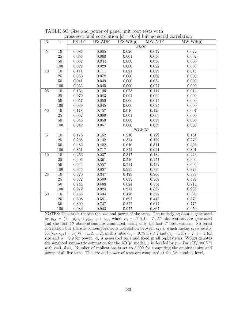
TABLE 6C: Size and power of panel unit root tests withcross-sectional correlation [σ = 0.75] but no serial correlation


5 10 0.086 0.085 0.026 0.072 0.02225 0.056 0.060 0.001 0.050 0.00250 0.032 0.044 0.000 0.036 0.000100 0.022 0.029 0.000 0.022 0.000

10 10 0.111 0.111 0.021 0.089 0.01525 0.063 0.078 0.000 0.060 0.00050 0.041 0.049 0.000 0.034 0.000100 0.033 0.040 0.000 0.027 0.000

25 10 0.134 0.146 0.023 0.117 0.01425 0.070 0.083 0.001 0.062 0.00050 0.057 0.059 0.000 0.044 0.000100 0.039 0.045 0.000 0.035 0.000

50 10 0.118 0.157 0.016 0.123 0.00725 0.062 0.089 0.001 0.069 0.00050 0.046 0.059 0.000 0.039 0.000100 0.042 0.057 0.000 0.039 0.000

POWER5 10 0.176 0.152 0.210 0.129 0.161

25 0.268 0.142 0.374 0.189 0.27650 0.482 0.402 0.616 0.311 0.493100 0.851 0.717 0.874 0.621 0.801

10 10 0.263 0.237 0.317 0.182 0.24325 0.406 0.361 0.520 0.257 0.39450 0.634 0.557 0.734 0.432 0.603100 0.933 0.837 0.935 0.733 0.878

25 10 0.370 0.347 0.423 0.260 0.33925 0.522 0.509 0.633 0.369 0.49950 0.744 0.688 0.824 0.554 0.714100 0.972 0.924 0.971 0.837 0.936

50 10 0.456 0.434 0.476 0.322 0.39025 0.608 0.581 0.697 0.442 0.57350 0.809 0.747 0.877 0.617 0.775100 0.983 0.943 0.977 0.867 0.950


30

TABLE 7: Size and power of panel unit root tests withboth cross-sectional correlation [σ = 0.5] and serial correlation


5 10 0.074 0.074 0.012 0.071 0.01225 0.060 0.035 0.001 0.033 0.00050 0.045 0.019 0.000 0.017 0.000100 0.035 0.011 0.000 0.011 0.000

10 10 0.089 0.088 0.010 0.085 0.00725 0.064 0.040 0.000 0.038 0.00050 0.061 0.025 0.000 0.021 0.000100 0.045 0.017 0.000 0.016 0.000

25 10 0.097 0.092 0.004 0.086 0.00325 0.060 0.042 0.000 0.040 0.00050 0.052 0.028 0.000 0.024 0.000100 0.053 0.021 0.000 0.016 0.000

50 10 0.108 0.108 0.008 0.108 0.00425 0.068 0.045 0.000 0.038 0.00050 0.063 0.032 0.000 0.026 0.000100 0.053 0.024 0.000 0.020 0.000

POWER5 10 0.045 0.123 0.143 0.112 0.114

25 0.042 0.186 0.309 0.147 0.23750 0.075 0.352 0.594 0.272 0.486100 0.254 0.760 0.910 0.663 864

10 10 0.057 0.179 0.219 0.147 0.17725 0.068 0.299 0.474 0.213 0.36650 0.118 0.562 0.774 0.433 0.668100 0.464 0.900 0.970 0.811 0.945

25 10 0.097 0.271 0.336 0.227 0.26925 0.101 0.489 0.653 0.357 0.53650 0.240 0.754 0.890 0.616 0.816100 0.683 0.972 0.991 0.927 0.982

50 10 0.122 0.364 0.420 0.299 0.35325 0.148 0.604 0.728 0.454 0.63750 0.318 0.833 0.930 0.710 0.886100 0.823 0.982 0.992 0.950 0.989

NOTES: This table reports the size and power of the tests. The underlying data is generatedby yi,t = (1 − ρ)αi + ρyi,t−1 + εi,t, where αi ∼ U [0, 1]. T+50 observations are generated andthe first 50 observations are eliminated, using only the last T observations. There are bothserial correlation and contemporaneous correlation between εi,t’s, which means: εi,t = λiεi,t−1+ui,t where λi ∼ U [0.2, 0.4] and ui,t’s satisfy the contemporaneous correlation cov(ui,t, uj,t) =σij ,∀t = 1, 2, ..., T , in this table σij = 0.5 if i 6= j and σij = 1 if i = j. ρ = 1 for size andρ = 0.9 for power. αi and λi are generated once and fixed in all replications. WS(p) denotesthe weighted symmetric estimation for the AR(p) model, p is decided by p = Int[c(T/100)1/d]with c=4, d=4. Number of replications is set to 3,000 for computing the empirical size andpower of all five tests. The size and power of tests are computed at the 5% nominal level.

31

Documents

Panel Data Unit Roots Tests Using Various Estimation Methodsspot.colorado.edu/~mcnownr/working_papers/panel-unit-root-tests.pdf · Panel Data Unit Roots Tests Using Various Estimation