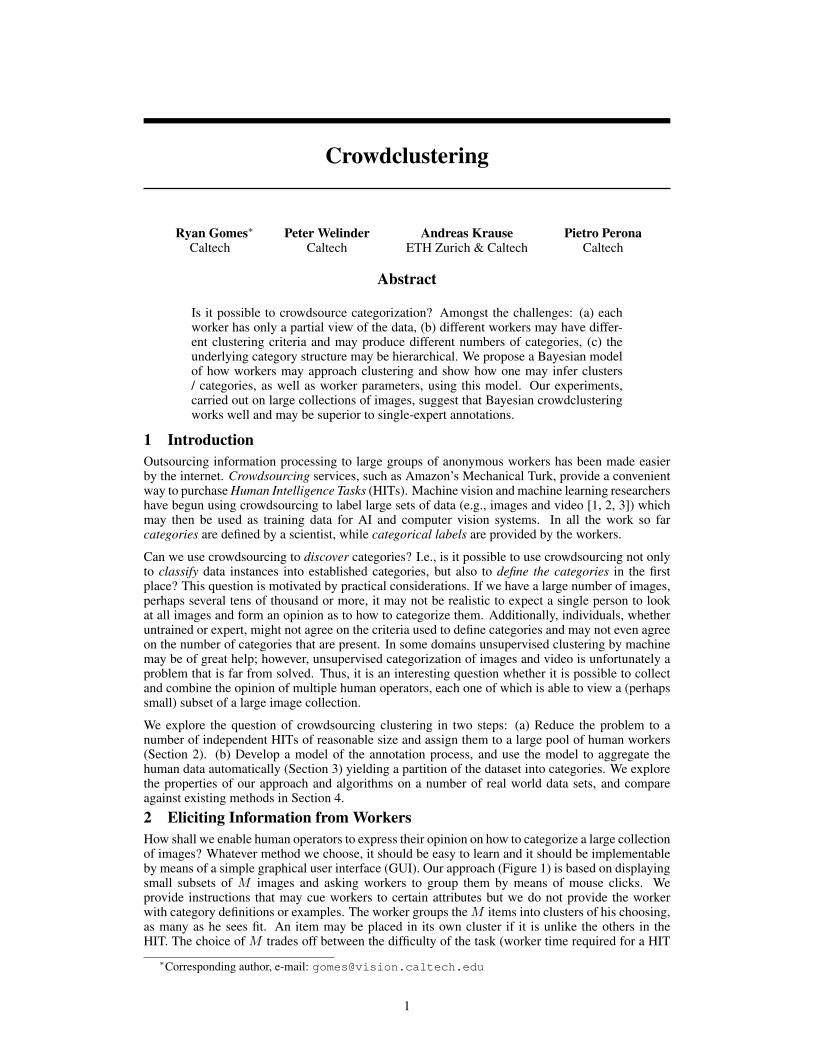
Crowdclustering

Ryan Gomes∗Caltech

Peter WelinderCaltech

Andreas KrauseETH Zurich & Caltech

Pietro PeronaCaltech

Abstract

Is it possible to crowdsource categorization? Amongst the challenges: (a) eachworker has only a partial view of the data, (b) different workers may have differ-ent clustering criteria and may produce different numbers of categories, (c) theunderlying category structure may be hierarchical. We propose a Bayesian modelof how workers may approach clustering and show how one may infer clusters/ categories, as well as worker parameters, using this model. Our experiments,carried out on large collections of images, suggest that Bayesian crowdclusteringworks well and may be superior to single-expert annotations.

1 IntroductionOutsourcing information processing to large groups of anonymous workers has been made easierby the internet. Crowdsourcing services, such as Amazon’s Mechanical Turk, provide a convenientway to purchase Human Intelligence Tasks (HITs). Machine vision and machine learning researchershave begun using crowdsourcing to label large sets of data (e.g., images and video [1, 2, 3]) whichmay then be used as training data for AI and computer vision systems. In all the work so farcategories are defined by a scientist, while categorical labels are provided by the workers.

Can we use crowdsourcing to discover categories? I.e., is it possible to use crowdsourcing not onlyto classify data instances into established categories, but also to define the categories in the firstplace? This question is motivated by practical considerations. If we have a large number of images,perhaps several tens of thousand or more, it may not be realistic to expect a single person to lookat all images and form an opinion as to how to categorize them. Additionally, individuals, whetheruntrained or expert, might not agree on the criteria used to define categories and may not even agreeon the number of categories that are present. In some domains unsupervised clustering by machinemay be of great help; however, unsupervised categorization of images and video is unfortunately aproblem that is far from solved. Thus, it is an interesting question whether it is possible to collectand combine the opinion of multiple human operators, each one of which is able to view a (perhapssmall) subset of a large image collection.

We explore the question of crowdsourcing clustering in two steps: (a) Reduce the problem to anumber of independent HITs of reasonable size and assign them to a large pool of human workers(Section 2). (b) Develop a model of the annotation process, and use the model to aggregate thehuman data automatically (Section 3) yielding a partition of the dataset into categories. We explorethe properties of our approach and algorithms on a number of real world data sets, and compareagainst existing methods in Section 4.

2 Eliciting Information from WorkersHow shall we enable human operators to express their opinion on how to categorize a large collectionof images? Whatever method we choose, it should be easy to learn and it should be implementableby means of a simple graphical user interface (GUI). Our approach (Figure 1) is based on displayingsmall subsets of M images and asking workers to group them by means of mouse clicks. Weprovide instructions that may cue workers to certain attributes but we do not provide the workerwith category definitions or examples. The worker groups theM items into clusters of his choosing,as many as he sees fit. An item may be placed in its own cluster if it is unlike the others in theHIT. The choice of M trades off between the difficulty of the task (worker time required for a HIT

∗Corresponding author, e-mail: gomes@vision.caltech.edu

1

Image set Annotators

GUI

Pairwise labels

6=

6=

6= ltτj

xi

Wj

zi

atbtjt

Annotators

Data Items

Pairwise Labels

Φk

Vk

“Atom

ic” clusters

Model / inference Categories

Figure 1: Schematic of Bayesian crowdclustering. A large image collection is explored by workers. In eachHIT (Section 2), the worker views a small subset of images on a GUI. By associating (arbitrarily chosen)colors with sets of images the worker proposes a (partial) local clustering. Each HIT thus produces multiplebinary pairwise labels: each pair of images shown in the same HIT is placed by the worker either in the samecategory or in different categories. Each image is viewed by multiple workers in different contexts. A modelof the annotation process (Sec. 3.1) is used to compute the most likely set of categories from the binary labels.Worker parameters are estimated as well.

increases super-linearly with the number of items), the resolution of the images (more images on thescreen means that they will be smaller), and contextual information that may guide the worker tomake more global category decisions (more images give a better context). We will further addressthe issue of context in Section 4.1. Partial clusterings on many M -sized subsets of the data frommany different workers are thus the raw data on which we compute clustering.

An alternative would have been to use pairwise distance judgments or three-way comparisons. Alarge body of work exists in the social sciences that makes use of human-provided similarity valuesdefined between pairs of data items (e.g., Multidimensional Scaling [4].) After obtaining pairwisesimilarity ratings from workers, and producing a Euclidean embedding, one could conceivably pro-ceed with unsupervised clustering of the data in the Euclidean space. However, accurate distancejudgments may be more laborious to specify than partial clusterings. We chose to explore what wecan achieve with partial clusterings alone.

We do not expect workers to agree on their definitions of categories, or to be consistent in catego-rization when performing multiple HITs. Thus, we avoid explicitly associating categories acrossHITs. Instead, we represent the results of each HIT as a series of

(M2

)binary labels (see Figure 1).

We assume that there are N total items (indexed by i), J workers (indexed by j), and H HITs(indexed by h). The information obtained from workers is a set of binary variables L, with ele-ments lt ∈ −1,+1 indexed by a positive integer t ∈ 1, . . . , T. Associated with the t-th labelis a quadruple (at, bt, jt, ht), where jt ∈ 1, . . . , J indicates the worker that produced the label,and at ∈ 1, . . . , N and bt ∈ 1, . . . , N indicate the two data items compared by the label.ht ∈ 1, . . . ,H indicates the HIT from which the t-th pairwise label was derived. The number oflabels is T = H

(M2

).

Sampling Procedure We have chosen to structure HITs as clustering tasks of M data items, sowe must specify them. If we simply seperate the items into disjoint sets, then it will be impossible toinfer a clustering over the entire data set. We will not know whether two items in different HITs arein the same cluster or not. There must be some overlap or redundancy: data items must be membersof multiple HITs.

In the other extreme, we could construct HITs such that each pair of items may be found in at leastone HIT, so that every possible pairwise category relation is sampled. This would be quite expensivefor large number of items N , since the number of labels scales asymptotically as T ∈ Ω(N2).However, we expect a noisy transitive property to hold: if items a and b are likely to be in the samecluster, and items b and c are (not) likely in the same cluster, then items a and c are (not) likely tobe in the same cluster as well. The transitive nature of binary cluster relations should allow sparsesampling, especially when the number of clusters is relatively small.

As a baseline sampling method, we use the random sampling scheme outlined by Strehl andGhosh [5] developed for the problem of object distributed clustering, in which a partition of a com-plete data set is learned from a number of clusterings restricted to subsets of the data. (We compareour aggregation algorithm to this work in Section 4.) Their scheme controls the level of samplingredundancy with a single parameter V , which in our problem is interpreted as the expected numberof HITs to which a data item belongs.

2

The N items are first distributed deterministically among the HITs, so that there are dMV e itemsin each HIT. Then the remaining M − dMV e items in each HIT are filled by sampling without re-placement from the N − dMV e items that are not yet allocated to the HIT. There are a total of dNVM eunique HITs. We introduce an additional parameterR, which is the number of different workers thatperform each constructed HIT. The total number of HITs distributed to the crowdsourcing service istherefore H = RdNVM e, and we impose the constraint that a worker can not perform the same HITmore than once. This sampling scheme generates T = RdNVM e

(M2

)∈ O(RNVM) binary labels.

With this exception, we find a dearth of ideas in the literature pertaining to sampling methods fordistributed clustering problems. Iterative schemes that adaptively choose maximally informativeHITs may be preferable to random sampling. We are currently exploring ideas in this direction.3 Aggregation via Bayesian CrowdclusteringThere is an extensive literature in machine learning on the problem of combining multiple alternativeclusterings of data. This problem is known as consensus clustering [6], clustering aggregation [7],or cluster ensembles [5]. While some of these methods can work with partial input clusterings, mosthave not been demonstrated in situations where the input clusterings involve only a small subset ofthe total data items (M << N ), which is the case in our problem.

In addition, existing approaches focus on producing a single “average” clustering from a set of inputclusterings. In contrast, we are not merely interested in the average clustering produced by a crowdof workers. Instead, we are interested in understanding the ways in which different individualsmay categorize the data. We seek a master clustering of the data that may be combined in order todescribe the tendencies of individual workers. We refer to these groups of data as atomic clusters.

For example, suppose one worker groups objects into a cluster of tall objects and another of shortobjects, while a different worker groups the same objects into a cluster of red objects and anotherof blue objects. Then, our method should recover four atomic clusters: tall red objects, short redobjects, tall blue objects, and short blue objects. The behavior of the two workers may then besummarized using a confusion table of the atomic clusters (see Section 3.3). The first worker groupsthe first and third atomic cluster into one category and the second and fourth atomic cluster intoanother category. The second worker groups the first and second atomic clusters into a category andthe third and fourth atomic clusters into another category.3.1 Generative ModelWe propose an approach in which data items are represented as points in a Euclidean space andworkers are modeled as pairwise binary classifiers in this space. Atomic clusters are then obtainedby clustering these inferred points using a Dirichlet process mixture model, which estimates thenumber of clusters [8]. The advantage of an intermediate Euclidean representation is that it providesa compact way to capture the characteristics of each data item. Certain items may be inherently moredifficult to categorize, in which case they may lie between clusters. Items may be similar along oneaxis but different along another (e.g., object height versus object color.) A similar approach wasproposed by Welinder et al. [3] for the analysis of classification labels obtained from crowdsourcingservices. This method does not apply to our problem, since it involves binary labels applied to singledata items rather than to pairs, and therefore requires that categories be defined a priori and agreedupon by all workers, which is incompatible with the crowdclustering problem.

We propose a probabilistic latent variable model that relates pairwise binary labels to hidden vari-ables associated with both workers and images. The graphical model is shown in Figure 1. xiis a D dimensional vector, with components [xi]d that encodes item i’s location in the embed-ding space RD. Symmetric matrix Wj ∈ RD×D with entries [Wj ]d1d2 and bias τj ∈ R areused to define a pairwise binary classifier, explained in the next paragraph, that represents workerj’s labeling behavior. Because Wj is symmetric, we need only specify its upper triangular por-tion: vecpWj which is a vector formed by “stacking” the partial columns of Wj accordingto the ordering [vecpWj]1 = [Wj ]11, [vecpWj]2 = [Wj ]12, [vecpWj]3 = [Wj ]22, etc.Φk = µk,Σk are the mean and covariance parameters associated with the k-th Gaussian atomiccluster, and Uk are stick breaking weights associated with a Dirichlet process.

The key term is the pairwise quadratic logistic regression likelihood that captures worker j’s ten-dency to label the pair of images at and bt with lt:

p(lt|xat ,xbt ,Wjt , τjt) =1

1 + exp(−ltAt)(1)

3

where we define the pairwise quadratic activity At = xTatWjtxbt + τjt . Symmetry of Wj ensuresthat p(lt|xat ,xbt ,Wjt , τjt) = p(lt|xbt ,xat ,Wjt , τjt). This form of likelihood yields a compactand tractable method of representing classifiers defined over pairs of points in Euclidean space.Pairs of vectors with large pairwise activity tend to be classified as being in the same category,and in different categories otherwise. We find that this form of likelihood leads to tightly groupedclusters of points xi that are then easily discovered by mixture model clustering.

The joint distribution is

p(Φ, U, Z,X,W, τ,L) =

∞∏k=1

p(Uk|α)p(Φk|m0, β0,J0, η0)

N∏i=1

p(zi|U)p(xi|Φzi) (2)

J∏j=1

p(vecpWj|σw0 )p(τj |στ0 )

T∏t=1

p(lt|xat ,xbt ,Wjt , τjt).

The conditional distributions are defined as follows:

p(Uk|α) = Beta(Uk; 1, α) p(zi = k|U) = Uk

k−1∏l=1

(1− Ul) (3)

p(xi|Φzi) = Normal(xi;µzi ,Σzi) p(xi|σx0 ) =∏d

Normal([xi]d; 0, σx0 )

p(vecpWj|σw0 ) =∏d1≤d2

Normal([Wj ]d1d2 ; 0, σw0 ) p(τj |στ0 ) = Normal(τj ; 0, στ0 )

p(Φk|m0, β0,J0, η0) = Normal-Wishart(Φk; m0, β0,J0, η0)

where (σx0 , στ0 , σ

w0 , α,m0, β0,J0, η0) are fixed hyper-parameters. Our model is similar to that

of [9], which is used to model binary relational data. Salient differences include our use of a logisticrather than a Gaussian likelihood, and our enforcement of the symmetry of Wj . In the next section,we develop an efficient deterministic inference algorithm to accomodate much larger data sets thanthe sampling algorithm used in [9].

3.2 Approximate InferenceExact posterior inference in this model is intractable, since computing it involves integrating overvariables with complex dependencies. We therefore develop an inference algorithm based on theVariational Bayes method [10]. The high level idea is to work with a factorized proxy posteriordistribution that does not model the full complexity of interactions between variables; it insteadrepresents a single mode of the true posterior. Because this distribution is factorized, integrationsinvolving it become tractable. We define the proxy distribution q(Φ, U, Z,X,W, τ) =

∞∏k=K+1

p(Uk|α)p(Φk|m0, β0,J0, η0)K∏k=1

q(Uk)q(Φk)N∏i=1

q(zi)q(xi)J∏j=1

q(vecpWj)q(τj) (4)

using parametric distributions of the following form:

q(Uk) = Beta(Uk; ξk,1, ξk,2) q(Φk) = Normal-Wishart(mk, βk,Jk, ηk) (5)

q(xi) =∏d

Normal([xi]d; [µxi ]d, [σxi ]d) q(τj) = Normal(τj ;µτj , σ

τj )

q(zi = k) = qik q(vecpWj) =∏d1≤d2

Normal([Wj ]d1d2 ; [µwj ]d1d2 , [σwj ]d1d2)

To handle the infinite number of mixture components, we follow the approach of [11] where wedefine variational distributions for the firstK components, and fix the remainder to their correspond-ing priors. ξk,1, ξk,2 and mk, βk,Jk, ηk are the variational parameters associated with the k-thmixture component. q(zi = k) = qik form the factorized assignment distribution for item i. µxi andσxi are variational mean and variance parameters associated with data item i’s embedding location.µwj and σwj are symmetric matrix variational mean and variance parameters associated with workerj, and µτj and στj are variational mean and variance parameters for the bias τj of worker j. We usediagonal covariance Normal distributions over Wj and xi to reduce the number of parameters thatmust be estimated.

4

Next, we define a utility function which allows us to determine the variational parameters. We useJensen’s inequality to develop a lower bound to the log evidence:

log p(L|σx0 , στ0 , σw0 , α,m0, β0,J0, η0) (6)≥Eq log p(Φ, U, Z,X,W, τ,L) +Hq(Φ, U, Z,X,W, τ),

H· is the entropy of the proxy distribution, and the lower bound is know as the Free Energy.However, the Free Energy still involves intractable integration, because the normal distributionsover variables Wj , xi, and τj are not conjugate [12] to the logistic likelihood term. We thereforelocally approximate the logistic likelihood with an unnormalized Gaussian function lower bound,which is the left hand side of the following inequality:

g(∆t) exp(ltAt −∆t)/2 + λ(∆t)(A2t −∆2

t ) ≤ p(lt|xat ,xbt ,Wjt , τjt). (7)

This was adapted from [13] to our case of quadratic pairwise logistic regression. Here g(x) =(1 + e−x)−1 and λ(∆) = [1/2− g(∆)]/(2∆). This expression introduces an additional variationalparameter ∆t for each label, which are optimized in order to tighten the lower bound. Our utilityfunction is therefore:

F =Eq log p(Φ, U, Z,X,W, τ) +Hq(Φ, U, Z,X,W, τ) (8)

+∑t

log g(∆t) +lt2EqAt −

∆t

2+ λ(∆t)(EqA2

t −∆2t )

which is a tractable lower bound to the log evidence. Optimization of variational parameters iscarried out in a coordinate ascent procedure, which exactly maximizes each variational parameter inturn while holding all others fixed. This is guaranteed to converge to a local maximum of the utilityfunction. The update equations are given in an extended technical report [14]. We initialize the vari-ational parameters by carrying out a layerwise procedure: first, we substitute a zero mean isotropicnormal prior for the mixture model and perform variational updates over µxi ,σxi ,µwj ,σwj , µτj , στj .Then we use µxi as point estimates for xi and update mk, βk,Jk, ηk, ξk,1, ξk,2 and determine theinitial number of clusters K as in [11]. Finally, full joint inference updates are performed. Theircomputational complexity is O(D4T +D2KN) = O(D4NV RM +D2KN).

3.3 Worker Confusion AnalysisAs discussed in Section 3, we propose to understand a worker’s behavior in terms of how he groupsatomic clusters into his own notion of categories. We are interested in the predicted confusion matrixCj for worker j, where

[Cj ]k1k2 = Eq

∫p(l = 1|xa,xb,Wj , τj)p(xa|Φk1)p(xb|Φk2)dxadxb

(9)

which expresses the probability that worker j assigns data items sampled from atomic cluster k1and k2 to the same cluster, as predicted by the variational posterior. This integration is intractable.We use the expected values EΦk1 = mk1 ,Jk1/ηk1 and EΦk2 = mk2 ,Jk2/ηk2 as pointestimates in place of the variational distributions over Φk1 and Φk2 . We then use Jensen’s inequalityand Eq. 7 again to yield a lower bound. Maximizing this bound over ∆ yields

[Cj ]k1k2 = g(∆k1k2j) exp(mTk1µ

wj mk2 + µτj − ∆k1k2j)/2 (10)

which we use as our approximate confusion matrix, where ∆k1k2j is given in [14].

4 ExperimentsWe tested our method on four image data sets that have established “ground truth” categories, whichwere provided by a single human expert. These categories do not necessarily reflect the uniquelyvalid way to categorize the data set, however they form a convenient baseline for the purpose ofquantitative comparison. We used 1000 images from the Scenes data set from [15] to illustrate ourapproach (Figures 2, 3, and 4.) We used 1354 images of birds from 10 species in the CUB-200 dataset [16] (Table 1) and the 3845 images in the Stonefly9 data set [17] (Table 1) in order to compareour method quantitatively to other cluster aggregation methods. We used the 37794 images from theAttribute Discovery data set [18] in order to demonstrate our method on a large scale problem.

We set the dimensionality of xi to D = 4 (since higher dimensionality yielded no additional clus-ters) and we iterated the update equations 100 times, which was enough for convergence. Hyperpa-rameters were tuned once on synthetic pairwise labels that simulated 100 data points drawn from 4clusters, and fixed during all experiments.

5

−1.5 −1 −0.5 0 0.5 1 1.5−2.5

−2

−1.5

−1

−0.5

0

0.5

1Average assignment entropy (bits): 0.0029653

1 2

3

4

5

6

7 8

9

10 11

1

2

3

5

4

Gro

und

Tru

th

Inferred Cluster

1 2 3 4 5 6 7 8 9 10 11

bedroomsuburbkitchen

living roomcoastforest

highwayinside citymountain

open countrystreet

tall buildingoffice

0

10

20

30

40

50

60

70

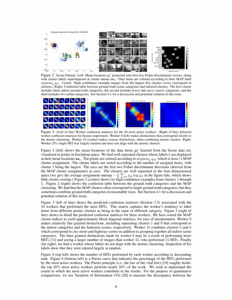
Figure 2: Scene Dataset. Left: Mean locations µxi projected onto first two Fisher discriminant vectors, along

with cluster labels superimposed at cluster means mk. Data items are colored according to their MAP labelargmaxk qik. Center: High confidence example images from the largest five clusters (rows correspond toclusters.) Right: Confusion table between ground truth scene categories and inferred clusters. The first clusterincludes three indoor ground truth categories, the second includes forest and open country categories, and thethird includes two urban categories. See Section 4.1 for a discussion and potential solution of this issue.

Worker: 9, # of HITs: 74

1 9 10 7 3 5 8 11 4 2 6

1

9

10

7

3

5

8

11

4

2

60

0.1

0.2

0.3

0.4

0.5

0.6

0.7

0.8

0.9

1Worker: 45, # of HITs: 15

1 9 7 10 3 5 8 11 4 6 2

1

9

7

10

3

5

8

11

4

6

2 0

0.1

0.2

0.3

0.4

0.5

0.6

0.7

0.8

0.9

1Worker: 29, # of HITs: 1

1 9 10 5 3 8 7 11 4 2 6

1

9

10

5

3

8

7

11

4

2

60

0.1

0.2

0.3

0.4

0.5

0.6

0.7

0.8

0.9

1

Figure 3: (Left of line) Worker confusion matrices for the 40 most active workers. (Right of line) Selectedworker confusion matrices for Scenes experiment. Worker 9 (left) makes distinctions that correspond closely tothe atomic clustering. Worker 45 (center) makes coarser distinctions, often combining atomic clusters. Right:Worker 29’s single HIT was largely random and does not align with the atomic clusters.

Figure 2 (left) shows the mean locations of the data items µxi learned from the Scene data set,visualized as points in Euclidean space. We find well seperated clusters whose labels k are displayedat their mean locations mk. The points are colored according to argmaxk qik, which is item i’s MAPcluster assignment. The cluster labels are sorted according to the number of assigned items, withcluster 1 being the largest. The axes are the first two Fisher discriminant directions (derived fromthe MAP cluster assignments) as axes. The clusters are well seperated in the four dimensionsalspace (we give the average assignment entropy − 1

N

∑ik qik log qik in the figure title, which shows

little cluster overlap.) Figure 2 (center) shows six high confidence examples from clusters 1 through5. Figure 2 (right) shows the confusion table between the ground truth categories and the MAPclustering. We find that the MAP clusters often correspond to single ground truth categories, but theysometimes combine ground truth categories in reasonable ways. See Section 4.1 for a discussion andpotential solution of this issue.

Figure 3 (left of line) shows the predicted confusion matrices (Section 3.3) associated with the40 workers that performed the most HITs. This matrix captures the worker’s tendency to labelitems from different atomic clusters as being in the same or different category. Figure 3 (right ofline) shows in detail the predicted confusion matrices for three workers. We have sorted the MAPcluster indices to yield approximately block diagonal matrices, for ease of interpretation. Worker 9makes relatively fine grained distinctions, including seperating clusters 1 and 9 that correspond tothe indoor categories and the bedroom scenes, respectively. Worker 45 combines clusters 5 and 8which correspond to city street and highway scenes in addition to grouping together all indoor scenecategories. The finer grained distinctions made by worker 9 may be a result of performing moreHITs (74) and seeing a larger number of images than worker 45, who performed 15 HITs. Finally(far right), we find a worker whose labels do not align with the atomic clustering. Inspection of hislabels show that they were entered largely at random.

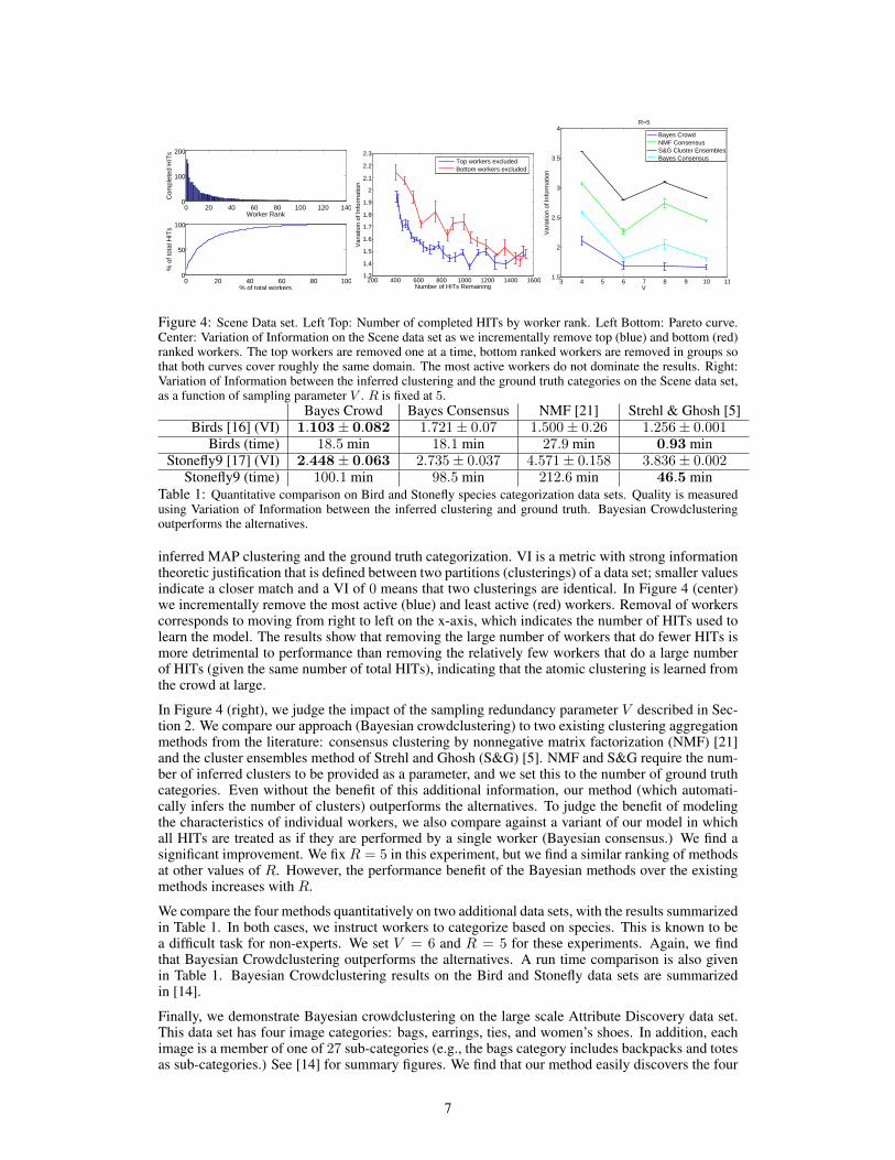
Figure 4 (top left) shows the number of HITs performed by each worker according to descendingrank. Figure 4 (bottom left) is a Pareto curve that indicates the percentage of the HITs performedby the most active workers. The Pareto principle (i.e., the law of the vital few) [19] roughly holds:the top 20% most active workers perform nearly 80% of the work. We wish to understand theextent to which the most active workers contribute to the results. For the purpose of quantitativecomparisons, we use Variation of Information (VI) [20] to measure the discrepancy between the

6

0 20 40 60 80 100 120 1400

100

200

Worker Rank

Com

plet

ed H

ITs

0 20 40 60 80 1000

50

100

% of total workers

% o

f tot

al H

ITs

200 400 600 800 1000 1200 1400 16001.3

1.4

1.5

1.6

1.7

1.8

1.9

2

2.1

2.2

2.3

Var

iatio

n of

Info

rmat

ion

Number of HITs Remaining

Top workers excludedBottom workers excluded

3 4 5 6 7 8 9 10 111.5

2

2.5

3

3.5

4

V

Var

iatio

n of

Info

rmat

ion

R=5

Bayes CrowdNMF ConsensusS&G Cluster EnsemblesBayes Consensus

Figure 4: Scene Data set. Left Top: Number of completed HITs by worker rank. Left Bottom: Pareto curve.Center: Variation of Information on the Scene data set as we incrementally remove top (blue) and bottom (red)ranked workers. The top workers are removed one at a time, bottom ranked workers are removed in groups sothat both curves cover roughly the same domain. The most active workers do not dominate the results. Right:Variation of Information between the inferred clustering and the ground truth categories on the Scene data set,as a function of sampling parameter V . R is fixed at 5.

Bayes Crowd Bayes Consensus NMF [21] Strehl & Ghosh [5]Birds [16] (VI) 1.103± 0.082 1.721± 0.07 1.500± 0.26 1.256± 0.001

Birds (time) 18.5 min 18.1 min 27.9 min 0.93 minStonefly9 [17] (VI) 2.448± 0.063 2.735± 0.037 4.571± 0.158 3.836± 0.002

Stonefly9 (time) 100.1 min 98.5 min 212.6 min 46.5 minTable 1: Quantitative comparison on Bird and Stonefly species categorization data sets. Quality is measuredusing Variation of Information between the inferred clustering and ground truth. Bayesian Crowdclusteringoutperforms the alternatives.

inferred MAP clustering and the ground truth categorization. VI is a metric with strong informationtheoretic justification that is defined between two partitions (clusterings) of a data set; smaller valuesindicate a closer match and a VI of 0 means that two clusterings are identical. In Figure 4 (center)we incrementally remove the most active (blue) and least active (red) workers. Removal of workerscorresponds to moving from right to left on the x-axis, which indicates the number of HITs used tolearn the model. The results show that removing the large number of workers that do fewer HITs ismore detrimental to performance than removing the relatively few workers that do a large numberof HITs (given the same number of total HITs), indicating that the atomic clustering is learned fromthe crowd at large.

In Figure 4 (right), we judge the impact of the sampling redundancy parameter V described in Sec-tion 2. We compare our approach (Bayesian crowdclustering) to two existing clustering aggregationmethods from the literature: consensus clustering by nonnegative matrix factorization (NMF) [21]and the cluster ensembles method of Strehl and Ghosh (S&G) [5]. NMF and S&G require the num-ber of inferred clusters to be provided as a parameter, and we set this to the number of ground truthcategories. Even without the benefit of this additional information, our method (which automati-cally infers the number of clusters) outperforms the alternatives. To judge the benefit of modelingthe characteristics of individual workers, we also compare against a variant of our model in whichall HITs are treated as if they are performed by a single worker (Bayesian consensus.) We find asignificant improvement. We fix R = 5 in this experiment, but we find a similar ranking of methodsat other values of R. However, the performance benefit of the Bayesian methods over the existingmethods increases with R.

We compare the four methods quantitatively on two additional data sets, with the results summarizedin Table 1. In both cases, we instruct workers to categorize based on species. This is known to bea difficult task for non-experts. We set V = 6 and R = 5 for these experiments. Again, we findthat Bayesian Crowdclustering outperforms the alternatives. A run time comparison is also givenin Table 1. Bayesian Crowdclustering results on the Bird and Stonefly data sets are summarizedin [14].

Finally, we demonstrate Bayesian crowdclustering on the large scale Attribute Discovery data set.This data set has four image categories: bags, earrings, ties, and women’s shoes. In addition, eachimage is a member of one of 27 sub-categories (e.g., the bags category includes backpacks and totesas sub-categories.) See [14] for summary figures. We find that our method easily discovers the four

7

Original Cluster 1 Original Cluster 4 Original Cluster 8

Gro

und

Tru

th

Inferred Cluster

1 2 3

bedroomsuburbkitchen

living roomcoastforest

highwayinside citymountain

open countrystreet

tall buildingoffice

0

10

20

30

40

50

60

70

Gro

und

Tru

th

Inferred Cluster

1

bedroomsuburbkitchen

living roomcoastforest

highwayinside citymountain

open countrystreet

tall buildingoffice

0

10

20

30

40

50

60

70

Gro

und

Tru

th

Inferred Cluster

1 2 3

bedroomsuburbkitchen

living roomcoastforest

highwayinside citymountain

open countrystreet

tall buildingoffice

0

10

20

30

40

50

1.1

1.2

1.34.1

8.1

8.2

8.3

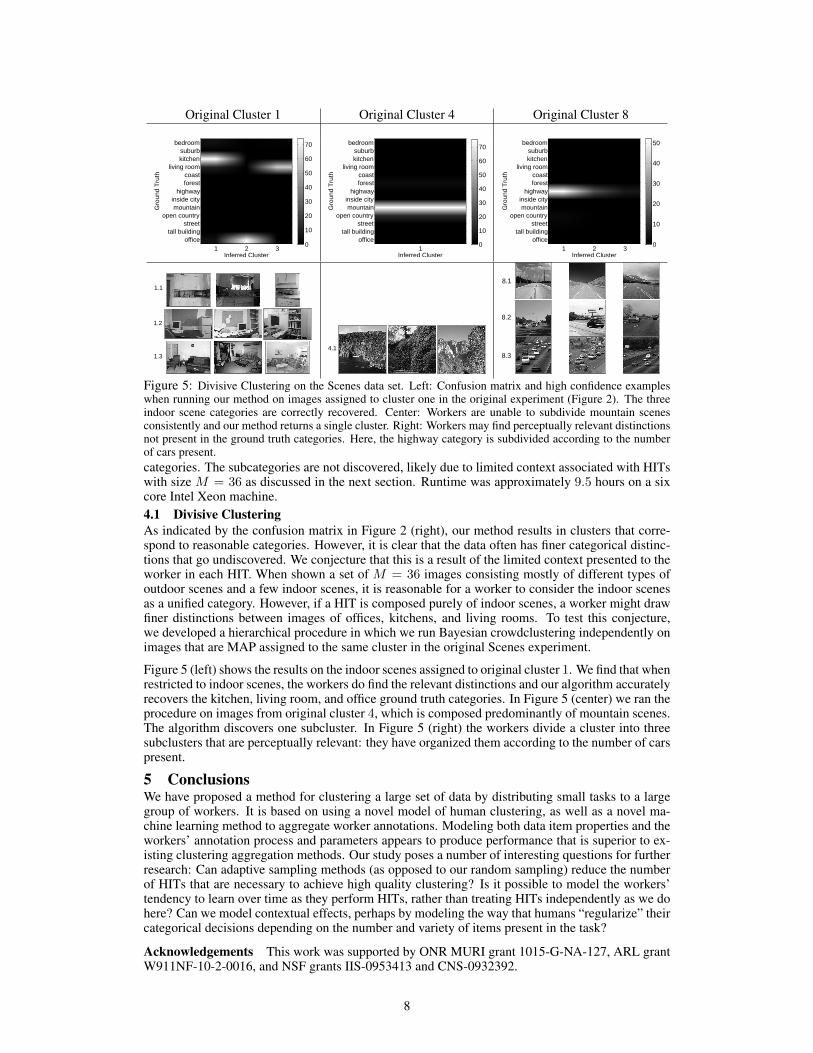
Figure 5: Divisive Clustering on the Scenes data set. Left: Confusion matrix and high confidence exampleswhen running our method on images assigned to cluster one in the original experiment (Figure 2). The threeindoor scene categories are correctly recovered. Center: Workers are unable to subdivide mountain scenesconsistently and our method returns a single cluster. Right: Workers may find perceptually relevant distinctionsnot present in the ground truth categories. Here, the highway category is subdivided according to the numberof cars present.categories. The subcategories are not discovered, likely due to limited context associated with HITswith size M = 36 as discussed in the next section. Runtime was approximately 9.5 hours on a sixcore Intel Xeon machine.4.1 Divisive ClusteringAs indicated by the confusion matrix in Figure 2 (right), our method results in clusters that corre-spond to reasonable categories. However, it is clear that the data often has finer categorical distinc-tions that go undiscovered. We conjecture that this is a result of the limited context presented to theworker in each HIT. When shown a set of M = 36 images consisting mostly of different types ofoutdoor scenes and a few indoor scenes, it is reasonable for a worker to consider the indoor scenesas a unified category. However, if a HIT is composed purely of indoor scenes, a worker might drawfiner distinctions between images of offices, kitchens, and living rooms. To test this conjecture,we developed a hierarchical procedure in which we run Bayesian crowdclustering independently onimages that are MAP assigned to the same cluster in the original Scenes experiment.

Figure 5 (left) shows the results on the indoor scenes assigned to original cluster 1. We find that whenrestricted to indoor scenes, the workers do find the relevant distinctions and our algorithm accuratelyrecovers the kitchen, living room, and office ground truth categories. In Figure 5 (center) we ran theprocedure on images from original cluster 4, which is composed predominantly of mountain scenes.The algorithm discovers one subcluster. In Figure 5 (right) the workers divide a cluster into threesubclusters that are perceptually relevant: they have organized them according to the number of carspresent.

5 ConclusionsWe have proposed a method for clustering a large set of data by distributing small tasks to a largegroup of workers. It is based on using a novel model of human clustering, as well as a novel ma-chine learning method to aggregate worker annotations. Modeling both data item properties and theworkers’ annotation process and parameters appears to produce performance that is superior to ex-isting clustering aggregation methods. Our study poses a number of interesting questions for furtherresearch: Can adaptive sampling methods (as opposed to our random sampling) reduce the numberof HITs that are necessary to achieve high quality clustering? Is it possible to model the workers’tendency to learn over time as they perform HITs, rather than treating HITs independently as we dohere? Can we model contextual effects, perhaps by modeling the way that humans “regularize” theircategorical decisions depending on the number and variety of items present in the task?

Acknowledgements This work was supported by ONR MURI grant 1015-G-NA-127, ARL grantW911NF-10-2-0016, and NSF grants IIS-0953413 and CNS-0932392.

8

References

[1] A. Sorokin and D. A. Forsyth. Utility data annotation with Amazon Mechanical Turk. InInternet Vision, pages 1–8, 2008.

[2] Sudheendra Vijayanarasimhan and Kristen Grauman. Large-Scale Live Active Learning:Training Object Detectors with Crawled Data and Crowds. In CVPR, 2011.

[3] Peter Welinder, Steve Branson, Serge Belongie, and Pietro Perona. The multidimensionalwisdom of crowds. In Neural Information Processing Systems Conference (NIPS), 2010.

[4] J. B. Kruskal. Multidimensional scaling by optimizing goodness-of-fit to a nonmetric hypoth-esis. PSym, 29:1–29, 1964.

[5] Alexander Strehl and Joydeep Ghosh. Cluster ensembles—A knowledge reuse framework forcombining multiple partitions. Journal of Machine Learning Research, 3:583–617, 2002.

[6] Stefano Monti, Pablo Tamayo, Jill Mesirov, and Todd Golub. Consensus clustering: Aresampling-based method for class discovery and visualization of gene expression microar-ray data. Machine Learning, 52(1–2):91–118, 2003.

[7] Gionis, Mannila, and Tsaparas. Clustering aggregation. In ACM Transactions on KnowledgeDiscovery from Data, volume 1. 2007.

[8] A.Y. Lo. On a class of bayesian nonparametric estimates: I. density estimates. The Annals ofStatistics, pages 351–357, 1984.

[9] I. Sutskever, R. Salakhutdinov, and J.B. Tenenbaum. Modelling relational data using bayesianclustered tensor factorization. Advances in Neural Information Processing Systems (NIPS),2009.

[10] Hagai Attias. A variational baysian framework for graphical models. In NIPS, pages 209–215,1999.

[11] Kenichi Kurihara, Max Welling, and Nikos Vlassis. Accelerated variational dirichlet processmixtures. In B. Scholkopf, J. Platt, and T. Hoffman, editors, Advances in Neural InformationProcessing Systems 19. MIT Press, Cambridge, MA, 2007.

[12] J. M. Bernardo and A. F. M. Smith. Bayesian Theory. Wiley, 1994.[13] Tommi S. Jaakkola and Michael I. Jordan. A variational approach to Bayesian logistic regres-

sion models and their extensions, August 13 1996.[14] Ryan Gomes, Peter Welinder, Andreas Krause, and Pietro Perona. Crowdclustering. Technical

Report CaltechAUTHORS:20110628-202526159, June 2011.[15] Li Fei-Fei and Pietro Perona. A Bayesian hierarchical model for learning natural scene cate-

gories. In CVPR, pages 524–531. IEEE Computer Society, 2005.[16] P. Welinder, S. Branson, T. Mita, C. Wah, F. Schroff, S. Belongie, and P. Perona. Caltech-

UCSD Birds 200. Technical Report CNS-TR-2010-001, California Institute of Technology,2010.

[17] G. Martinez-Munoz, N. Larios, E. Mortensen, W. Zhang, A. Yamamuro, R. Paasch, N. Payet,D. Lytle, L. Shapiro, S. Todorovic, et al. Dictionary-free categorization of very similar objectsvia stacked evidence trees. 2009.

[18] T. Berg, A. Berg, and J. Shih. Automatic attribute discovery and characterization from noisyweb data. Computer Vision–ECCV 2010, pages 663–676, 2010.

[19] V. Pareto. Cours d’economie politique. 1896.[20] M. Meila. Comparing clusterings by the variation of information. In Learning theory and

Kernel machines: 16th Annual Conference on Learning Theory and 7th Kernel Workshop,COLT/Kernel 2003, Washington, DC, USA, August 24-27, 2003: proceedings, volume 2777,page 173. Springer Verlag, 2003.

[21] Tao Li, Chris H. Q. Ding, and Michael I. Jordan. Solving consensus and semi-supervisedclustering problems using nonnegative matrix factorization. In ICDM, pages 577–582. IEEEComputer Society, 2007.

9