1

CORROSION INHIBITORS IN CONCRETE

R.J. Kessler, R.G. Powers, and W.D. Cerlanek Florida Department of Transportation

State Materials Office 2006 NE Waldo Road Gainesville, FL 32609

A.A. Sagüés University of South Florida

Department of Civil and Environmental Engineering 4202 E Fowler Ave

ENB 118 Tampa, FL 33620-5350

ABSTRACT This report discusses the behavior of various corrosion inhibitors for steel in concrete. Three commercially available inhibitors (two based on organic compounds and one calcium nitrite-based) were selected for detailed examination. Each inhibitor was evaluated in several types of concrete mix designs. The mixes included Portland cement concrete as the control, concrete admixed with silica fume, and concrete admixed with fly ash for comparison. Non-destructive tests in progress of steel-reinforced concrete laboratory specimens are used to identify the time at which corrosion of the reinforcement initiates. Standard specimens containing either of the two organic corrosion inhibitors performed relatively equal to control specimens (Type II cement, no pozzolans, no inhibitors). Standard specimens containing the calcium nitrite-based inhibitor showed improved performance. However, specimens containing silica fume exhibit no corrosion activity to date. Based on current data, the calcium nitrite-based inhibitor was effective in mitigating corrosion in high permeability concretes. However, low-permeability concrete specimens containing pozzolans (particularly silica fume) continue to exhibit a significantly longer time to corrosion initiation than specimens containing only conventional corrosion inhibitors. Keywords: Concrete, corrosion, reinforcing steel, macrocell current, corrosion inhibitor, calcium nitrite, rebar, polarization, pozzolan

Paper No. 03288

2

INTRODUCTION The overall objective of this report is to discuss the behavior of selected commercially available corrosion inhibitors for steel in concrete. The extent to which these inhibitors prevent or slow down corrosion will be contrasted with the beneficial action of fly ash and silica fume. Unlike corrosion inhibitors, these pozzolanic admixtures do not directly influence the electrochemical corrosion reactions themselves, but nevertheless delay corrosion initiation by slowing down the ingress of chloride ions in concrete. The combined effect of the presence of corrosion inhibitors and pozzolanic admixtures will be discussed as well.

EXPERIMENTAL PROCEDURE Three commercially available corrosion inhibitors, one calcium nitrite-based (CN) and two based on organic compounds (ORG1, ORG2)(a), were selected for detailed examination1. For comparison, each inhibitor (plus blank controls) was admixed at recommended dosages per manufacturer guidelines(a) into several types of concrete mix designs, including Type II cement (American Association of State Highway and Transportation Officials [AASHTO] M 85) concrete, concrete admixed with silica fume, and concrete admixed with fly ash. The mixes to be discussed used 985 kg/m3 of oolitic limestone as coarse aggregate with a maximum diameter of 10 mm. The fine aggregate was silica sand with a fineness module of 2.16. The cementitious factor was 7 bags (390 kg/m3). The pozzolans were admixed as cement replacement in the percentages of 20% by weight of cement for Type F Fly Ash and 8% by weight of cement for silica fume. A summary of the proportions is shown in Table 1.

Table 1. Concrete Mix Proportions

7-Bag Std Mix Water/Cement Ratio

20% Fly Ash 8% Silica Fume

CTRL X 0.41 ORG1 X 0.41

CN X 0.41 ORG2 X 0.41

Fly Ash X 0.41 X Silica Fume X 0.41 X

The mixes were batched in a 27 ft3 (0.76 m3) central mixer, which is located in a warehouse environment. During extreme environmental conditions, batching was conducted in a temperature-controlled room, with a portable mixer. To maintain control of the w/c ratio, all components were carefully measured and aggregate moisture adjustments were made. Before batching, all aggregate was obtained from Florida Department of Transportation (FDOT) pre-qualified sources and tests were

(a) CN – DCI-S manufactured by W.R. Grace & Co, dosage – 22 liters per cubic meter of concrete. ORG1 – FerroGard 901 manufactured by Sika Corp, dosage – 9.9 liters per cubic meter of concrete. ORG2 – Rheocrete 222+ manufactured by Master Builders Technologies, dosage – 5.0 liters per cubic meter of concrete.

3

conducted to ascertain proper gradation. The aggregate was bagged and completely saturated by submerging the bagged materials in water. One hour before mixing, the bagged materials were removed from the water and allowed to drain. After mixing, the concrete was placed into the forms in two equal lifts. Using a table vibrator, the specimens were vibrated for 45 seconds per lift, to consolidate the concrete. Each specimen was light- trowel finished and the specimens were then covered with a polyethylene film for 24 hours. All specimens were cured in 100% relative humidity for 72 hours and further cured in a dry warehouse environment for a minimum of 90 days before testing commenced.

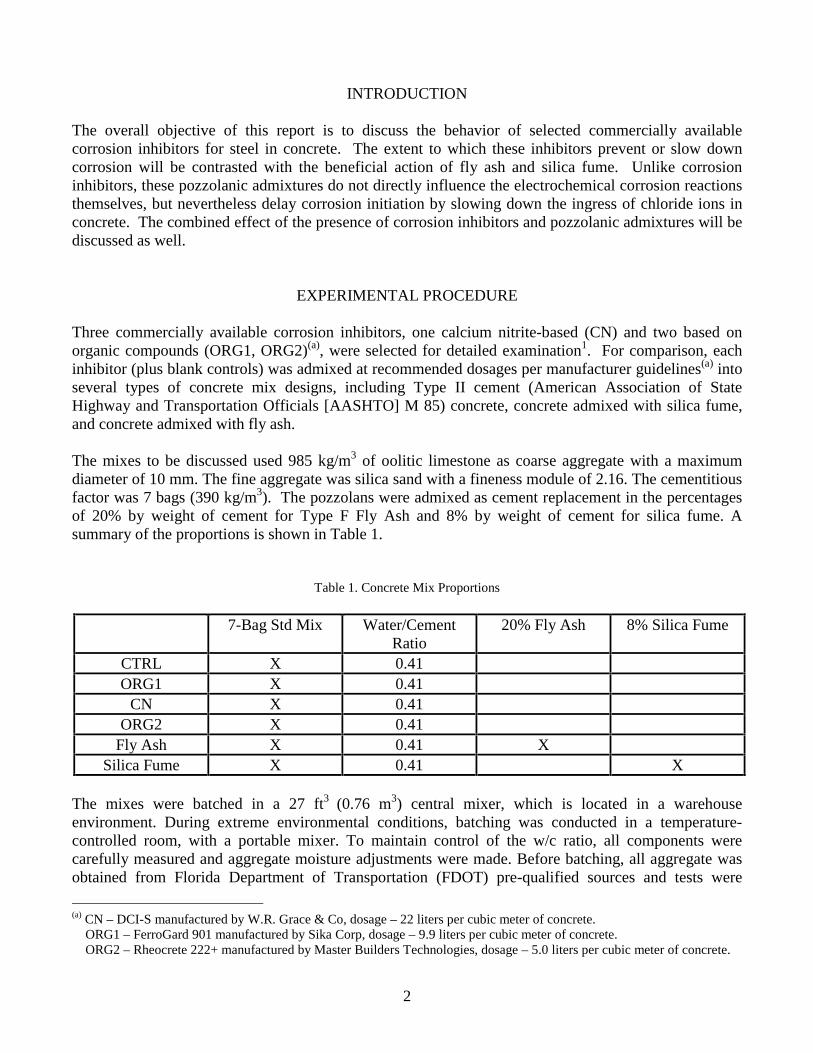
The specimens were manufactured to provide relatively short-term results, and were placed in a sheltered, outdoor exposure site. The arrangement of the specimens is shown in Figure 1 and the specimen configuration is shown in Figure 2. Conditions for exposure consisted of partial immersion, as seen in Figure 2. The water was a 3% NaCl solution. The specimen and tank temperatures depended on the fluctuations in the daily temperatures in Gainesville, FL. The four tanks are interconnected by water pipes and two pumps are used to circulate the saltwater. Twice daily, the water is circulated for one hour to ensure uniform chloride content within the tanks, and full aeration of the water. Water depth and salt content are measured weekly; each component is added, as necessary, to maintain the desired concentrations, and to maintain the desired water level. Routine specimen testing includes coupled and individual element half-cell potentials (using a standard calomel electrode, [SCE]), resistance to an external electrode, inter-element resistance, macrocell currents, polarization resistance, electrochemical impedance spectroscopy, and wet surface resistivity.

Figure 1. Sheltered outdoor specimens Figure 2. Schematic of outdoor specimens

Testing continues until specimen failure. Failure of a specimen is considered the point when a corrosion-induced crack is visually detected. Upon failure, specimens are removed from saltwater exposure and cores are taken from uncracked concrete for chloride analysis, which will be reported in a subsequent publication. Continuing work will also take into account the possible extent of inhibitor loss due to leaching out of the specimens during the tests2,3.

RESULTS AND DISCUSSION

This paper is based on the test results obtained from the ongoing Corrosion Inhibitors in Concrete1 project through September 2002. Each specimen was tested and monitored until visible indications of corrosion-induced cracking became evident on the surface of the specimen. Many of the specimens have advanced to failure and have been removed from the tanks. All that remain are those specimens admixed

4

with either silica fume or fly ash. The majority of the specimens remaining are those admixed with silica fume. Only a small percentage of specimens admixed with fly ash remain. Unfailed specimens remain under testing conditions.

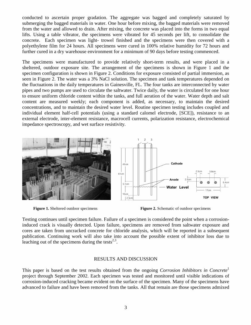
Figure 3. Average coupled (total) half-cell potentials to a SCE over time for all specimen groups. Comparisons Of Inhibitors And Pozzolanic Admixtures Acting Separately Figure 3 shows the evolution of the average coupled (total) half-cell potentials for all of the groups. The potentials shown are averages of all specimens of each group. Each curve terminates at the time the first failed specimen in a group was removed. Half-cell potential evolutions for all individual specimens of all relevant groups are provided in Appendix A. For comparison purposes, The Time to Corrosion Initiation (TCI) for a specimen was assumed to have been reached when the coupled half-cell potential crossed the nominal threshold value of –280 mV/SCE (which follows the commonly used assumption of a high probability of corrosion activity per ASTM C-876). By that criterion, the average potential trends in Figure 3 suggest representative TCI values for the specimen groups as shown in Table 2. It should be noted, based on the long-term potential data, that corrosion initiation likely occurred at a much earlier date than that corresponding to the nominal criterion used. As seen in the charts in Appendix A, a noticeable potential shift (~100 to 200 mV) occurs before the specimen potential reaches –280 mV. This shift more likely indicates the actual TCI for the specimen (average values for specimen groups are provided in Table 2). Thus, it is apparent that the –280 mV criterion produces an overestimate of the time to corrosion initiation for these specimens.

-500

-400

-300

-200

-100

0

100

0 200 400 600 800 1000 1200 1400 1600 1800 2000

Time (Days)

Po

ten

tial

s vs

SC

E (

mV

)

CTRL ORG1 CN ORG2 FA SF

CORROSION THRESHOLD = -280 mV

5

Table 2. Average TCI and Days to Failure for Specimen Groups

Sample Name

Mix Date Placement in

Saltwater

Average Time to First Significant Potential Drop

(Days)

Average TCI (–280 mV/SCE)

(Days)

Average Days to Failure*

Percent of Failed

Samples

CTRL 1/28/97 10/15/97 73 209 298 100 ORG1 1/22/97 10/15/97 140 245 418 100

CN 12/16/96 10/15/97 272 484 571 100 ORG2 1/30/97 10/15/97 120 168 279 100

Fly Ash 2/10/97 10/22/97 490 >757** >958** 80 Silica Fume 4/1/97 10/22/97 >1280** >1793** >1793** 0

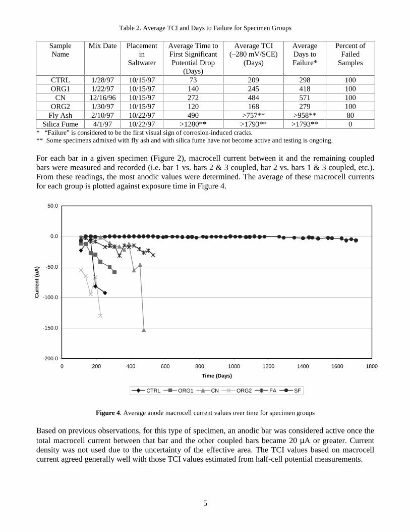
* “Failure” is considered to be the first visual sign of corrosion-induced cracks. ** Some specimens admixed with fly ash and with silica fume have not become active and testing is ongoing. For each bar in a given specimen (Figure 2), macrocell current between it and the remaining coupled bars were measured and recorded (i.e. bar 1 vs. bars 2 & 3 coupled, bar 2 vs. bars 1 & 3 coupled, etc.). From these readings, the most anodic values were determined. The average of these macrocell currents for each group is plotted against exposure time in Figure 4.

Figure 4. Average anode macrocell current values over time for specimen groups

Based on previous observations, for this type of specimen, an anodic bar was considered active once the total macrocell current between that bar and the other coupled bars became 20 µA or greater. Current density was not used due to the uncertainty of the effective area. The TCI values based on macrocell current agreed generally well with those TCI values estimated from half-cell potential measurements.

-200.0

-150.0

-100.0

-50.0

0.0

50.0

0 200 400 600 800 1000 1200 1400 1600 1800

Time (Days)

Cu

rren

t (u

A)

CTRL ORG1 CN ORG2 FA SF

6

The Rapid Chloride Permeability (RCP) test utilized was in accordance with American Society for Testing and Materials (ASTM) C 1202. The purpose of this test is to estimate the permeability of the concrete by measuring its conductivity. The 360-day tests showed lower results than the corresponding 28-day tests. This indicates that the concrete in the samples improved, which also indicates that the concrete continued to cure. The continual curing is also seen in the 28-day compression (ASTM C 39) results versus the 360-day compression results. Table 4 shows the results of the 28-day and 360-day results of both the RCP and the compressions tests.

Table 4. RCP and Compressions at 28 and 360 Days

Sample Name 28-Day RCP (Coulombs)

360-Day RCP (Coulombs)

28-Day Compression

(MPa)

360-Day Compression

(MPa) CTRL 5689 4448 47.8 53.0 ORG1 >12000 4710 51.6 57.4

CN N/A* N/A* 42.6 48.1 ORG2 9821 6943 36.9 41.8

Fly Ash 6793 1011 42.8 56.7 Silica Fume 1149 895 57.3 58.9

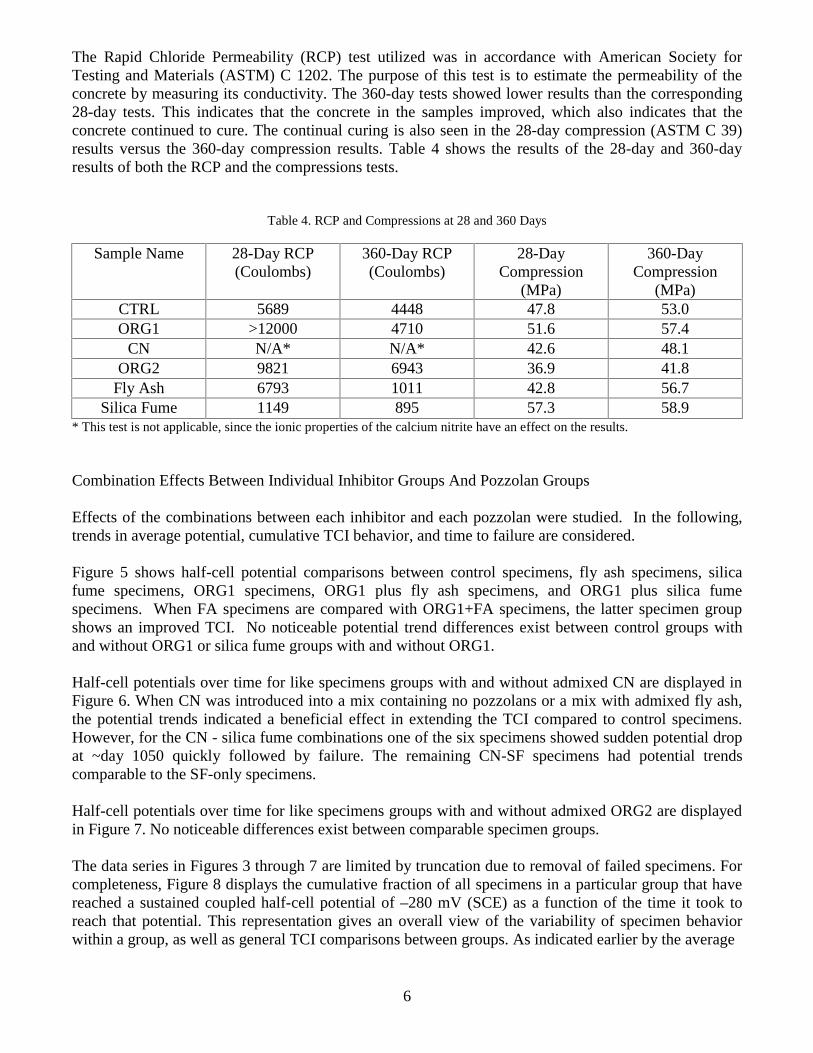
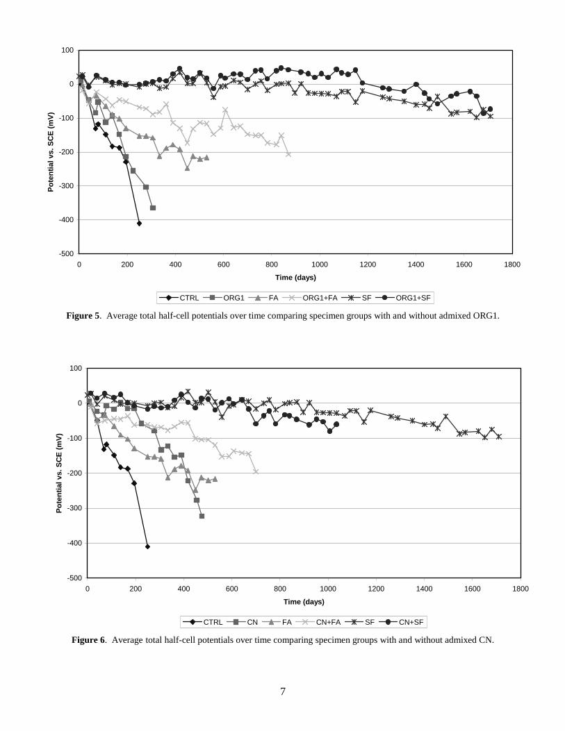
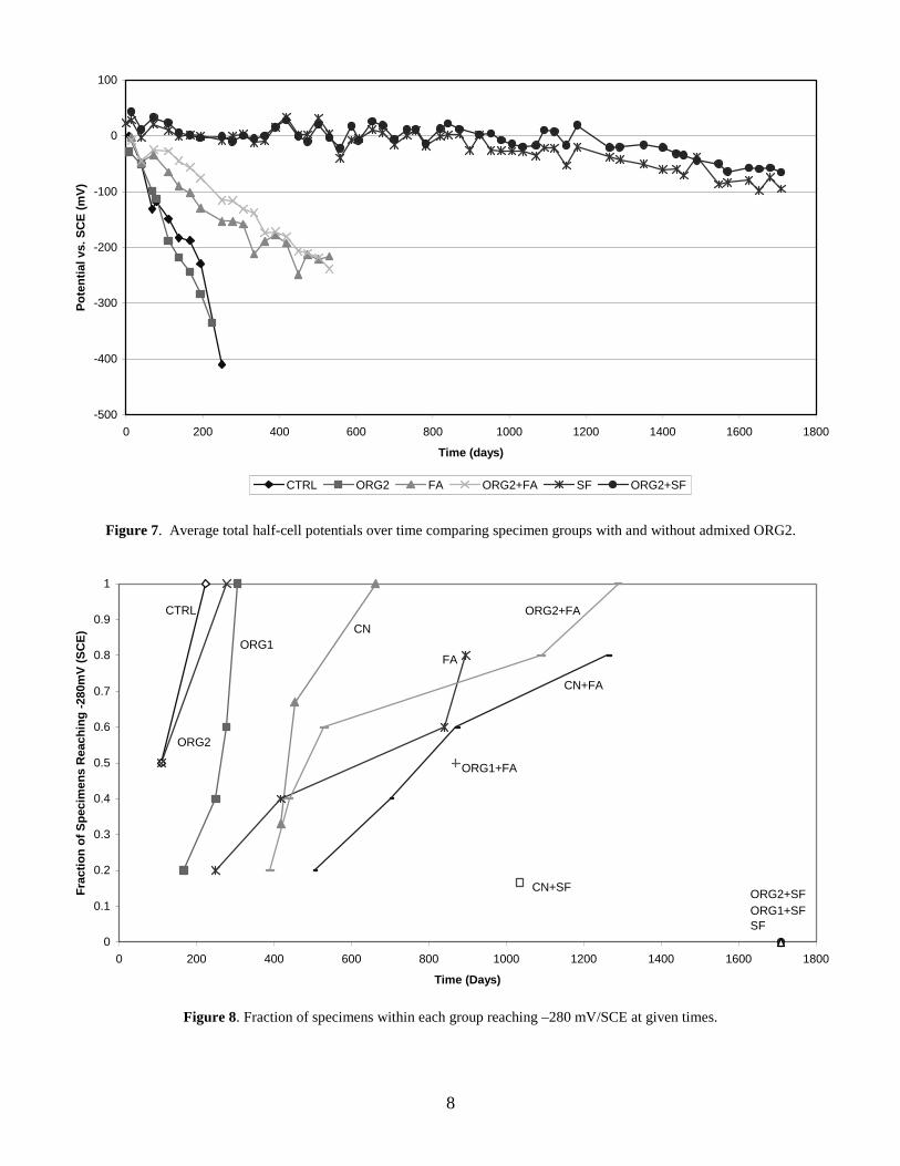
* This test is not applicable, since the ionic properties of the calcium nitrite have an effect on the results. Combination Effects Between Individual Inhibitor Groups And Pozzolan Groups Effects of the combinations between each inhibitor and each pozzolan were studied. In the following, trends in average potential, cumulative TCI behavior, and time to failure are considered. Figure 5 shows half-cell potential comparisons between control specimens, fly ash specimens, silica fume specimens, ORG1 specimens, ORG1 plus fly ash specimens, and ORG1 plus silica fume specimens. When FA specimens are compared with ORG1+FA specimens, the latter specimen group shows an improved TCI. No noticeable potential trend differences exist between control groups with and without ORG1 or silica fume groups with and without ORG1. Half-cell potentials over time for like specimens groups with and without admixed CN are displayed in Figure 6. When CN was introduced into a mix containing no pozzolans or a mix with admixed fly ash, the potential trends indicated a beneficial effect in extending the TCI compared to control specimens. However, for the CN - silica fume combinations one of the six specimens showed sudden potential drop at ~day 1050 quickly followed by failure. The remaining CN-SF specimens had potential trends comparable to the SF-only specimens. Half-cell potentials over time for like specimens groups with and without admixed ORG2 are displayed in Figure 7. No noticeable differences exist between comparable specimen groups. The data series in Figures 3 through 7 are limited by truncation due to removal of failed specimens. For completeness, Figure 8 displays the cumulative fraction of all specimens in a particular group that have reached a sustained coupled half-cell potential of –280 mV (SCE) as a function of the time it took to reach that potential. This representation gives an overall view of the variability of specimen behavior within a group, as well as general TCI comparisons between groups. As indicated earlier by the average

7

Figure 5. Average total half-cell potentials over time comparing specimen groups with and without admixed ORG1.

Figure 6. Average total half-cell potentials over time comparing specimen groups with and without admixed CN.

-500

-400

-300

-200

-100

0

100

0 200 400 600 800 1000 1200 1400 1600 1800

Time (days)

Po

ten

tial

vs.

SC

E (

mV

)

CTRL CN FA CN+FA SF CN+SF

-500

-400

-300

-200

-100

0

100

0 200 400 600 800 1000 1200 1400 1600 1800

Time (days)

Po

ten

tial

vs.

SC

E (

mV

)

CTRL ORG1 FA ORG1+FA SF ORG1+SF

8

Figure 7. Average total half-cell potentials over time comparing specimen groups with and without admixed ORG2.

Figure 8. Fraction of specimens within each group reaching –280 mV/SCE at given times.

-500

-400

-300

-200

-100

0

100

0 200 400 600 800 1000 1200 1400 1600 1800

Time (days)

Po

ten

tial

vs.

SC

E (

mV

)

CTRL ORG2 FA ORG2+FA SF ORG2+SF

0

0.1

0.2

0.3

0.4

0.5

0.6

0.7

0.8

0.9

1

0 200 400 600 800 1000 1200 1400 1600 1800

Time (Days)

Fra

ctio

n o

f S

pec

imen

s R

each

ing

-28

0mV

(S

CE

)

CTRL

ORG2

ORG1CN

ORG2+FA

FA

CN+FA

ORG1+FA

CN+SFORG2+SFORG1+SFSF

9

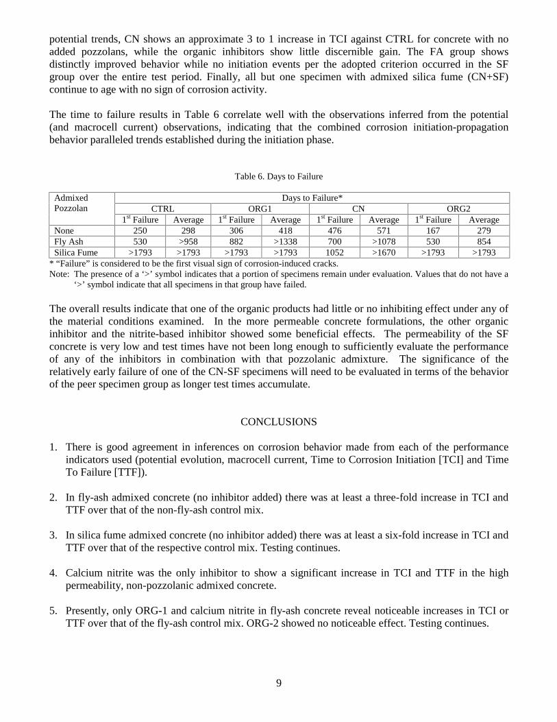
potential trends, CN shows an approximate 3 to 1 increase in TCI against CTRL for concrete with no added pozzolans, while the organic inhibitors show little discernible gain. The FA group shows distinctly improved behavior while no initiation events per the adopted criterion occurred in the SF group over the entire test period. Finally, all but one specimen with admixed silica fume (CN+SF) continue to age with no sign of corrosion activity. The time to failure results in Table 6 correlate well with the observations inferred from the potential (and macrocell current) observations, indicating that the combined corrosion initiation-propagation behavior paralleled trends established during the initiation phase.

Table 6. Days to Failure

Days to Failure* CTRL ORG1 CN ORG2

Admixed Pozzolan

1st Failure Average 1st Failure Average 1st Failure Average 1st Failure Average None 250 298 306 418 476 571 167 279 Fly Ash 530 >958 882 >1338 700 >1078 530 854 Silica Fume >1793 >1793 >1793 >1793 1052 >1670 >1793 >1793

* “Failure” is considered to be the first visual sign of corrosion-induced cracks. Note: The presence of a ‘>’ symbol indicates that a portion of specimens remain under evaluation. Values that do not have a

‘>’ symbol indicate that all specimens in that group have failed. The overall results indicate that one of the organic products had little or no inhibiting effect under any of the material conditions examined. In the more permeable concrete formulations, the other organic inhibitor and the nitrite-based inhibitor showed some beneficial effects. The permeability of the SF concrete is very low and test times have not been long enough to sufficiently evaluate the performance of any of the inhibitors in combination with that pozzolanic admixture. The significance of the relatively early failure of one of the CN-SF specimens will need to be evaluated in terms of the behavior of the peer specimen group as longer test times accumulate.

CONCLUSIONS 1. There is good agreement in inferences on corrosion behavior made from each of the performance

indicators used (potential evolution, macrocell current, Time to Corrosion Initiation [TCI] and Time To Failure [TTF]).

2. In fly-ash admixed concrete (no inhibitor added) there was at least a three-fold increase in TCI and TTF over that of the non-fly-ash control mix.

3. In silica fume admixed concrete (no inhibitor added) there was at least a six-fold increase in TCI and TTF over that of the respective control mix. Testing continues.

4. Calcium nitrite was the only inhibitor to show a significant increase in TCI and TTF in the high permeability, non-pozzolanic admixed concrete.

5. Presently, only ORG-1 and calcium nitrite in fly-ash concrete reveal noticeable increases in TCI or TTF over that of the fly-ash control mix. ORG-2 showed no noticeable effect. Testing continues.

10

6. None of the three inhibitors admixed in silica fume concrete presently reveal discernable behavior differences compared to their non-inhibitor added controls. Testing continues.

7. The –280 mV criterion produced overestimates of TCI based on comparisons with long-term

potential measurements.

NOTICE AND ACKNOWLEDGMENTS The assistance of Mario A. Paredes and Donna R. Fugatt of FDOT is gratefully acknowledged. The authors are also indebted to Dr. Y.P. Virmani for many helpful discussions. This investigation was conducted with support from the Federal Highway Administration and the FDOT. The opinions and findings indicated here are those of the authors and not necessarily those of the supporting organizations. The United States Government or the State of Florida assumes no liability for the content or use of this publication; it does not constitute a standard, specification, or regulation. The United States Government or the State of Florida does not endorse products or manufacturers. Trade and manufacturers’ names appear in this publication only because they are considered essential to the object of the document.

REFERENCES 1. R.G. Powers, A.A. Sagüés, W.D. Cerlanek, and C.A. Kasper, Corrosion Inhibitors in Concrete, Interim Report, pp. 32-52, Report Number FHWA-RD-02-002, National Information Service, Springfied, VA, 2002. 2. R.G. Powers, A.A. Sagüés, W.D. Cerlanek, C.A. Kasper and L. Li, Time to Corrosion of Reinforcing Steel in Concrete Containing Calcium Nitrite, U.S. Department of Transportation, FHWA Publication No. FHWA-RD-99-145, McLean, VA., October 1999. 3. H. Liang, L. Li, N.D. Poor, A.A. Sagüés, Cement and Concrete Research 33, pp.139–146, 2003.

11

Appendix A

12

-600

-500

-400

-300

-200

-100

0

100

0 100 200 300 400 500 600 700

Time (Days)

Po

ten

tial

vs.

SC

E (

mV

)

ORG1 A ORG1 B ORG1 C ORG1 D ORG1 E

Figure A-1. Potential evolution for individual CTRL specimens

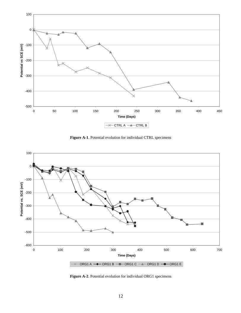
Figure A-2. Potential evolution for individual ORG1 specimens

-500

-400

-300

-200

-100

0

100

0 50 100 150 200 250 300 350 400 450

Time (Days)

Po

ten

tial

vs

SC

E (

mV

)

CTRL A CTRL B

13

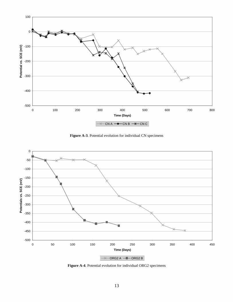
Figure A-3. Potential evolution for individual CN specimens

Figure A-4. Potential evolution for individual ORG2 specimens

-500

-400

-300

-200

-100

0

100

0 100 200 300 400 500 600 700 800

Time (Days)

Po

ten

tial

vs.

SC

E (

mV

)

CN A CN B CN C

-500

-450

-400

-350

-300

-250

-200

-150

-100

-50

0

0 50 100 150 200 250 300 350 400 450

Time (Days)

Po

ten

tial

s vs

. SC

E (

mV

)

ORG2 A ORG2 B

14

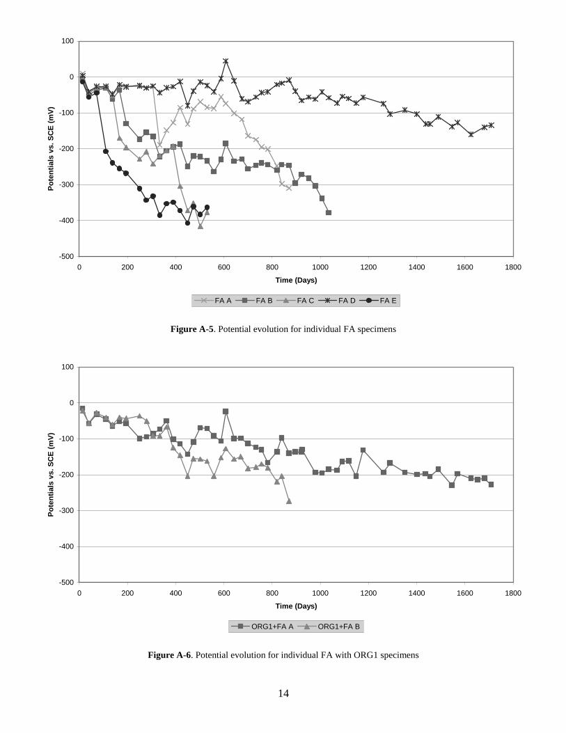
Figure A-5. Potential evolution for individual FA specimens

Figure A-6. Potential evolution for individual FA with ORG1 specimens

-500

-400

-300

-200

-100

0

100

0 200 400 600 800 1000 1200 1400 1600 1800

Time (Days)

Po

ten

tial

s vs

. SC

E (

mV

)

FA A FA B FA C FA D FA E

-500

-400

-300

-200

-100

0

100

0 200 400 600 800 1000 1200 1400 1600 1800

Time (Days)

Po

ten

tial

s vs

. SC

E (

mV

)

ORG1+FA A ORG1+FA B

15

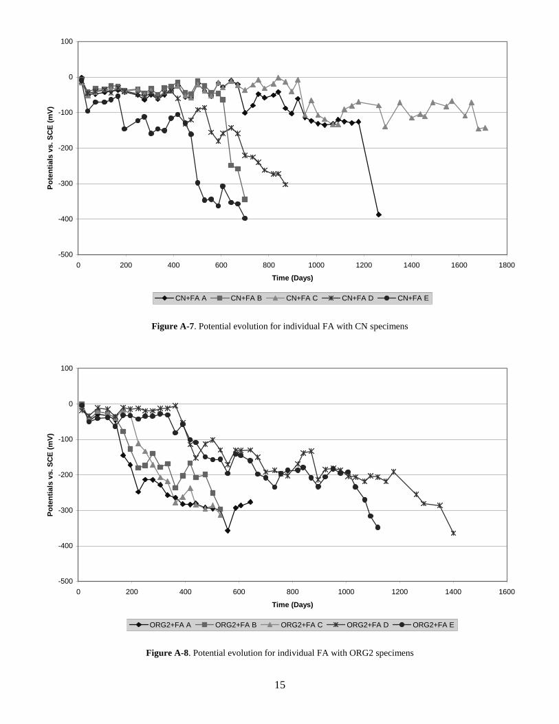
Figure A-7. Potential evolution for individual FA with CN specimens

Figure A-8. Potential evolution for individual FA with ORG2 specimens

-500

-400

-300

-200

-100

0

100

0 200 400 600 800 1000 1200 1400 1600 1800

Time (Days)

Po

ten

tial

s vs

. SC

E (

mV

)

CN+FA A CN+FA B CN+FA C CN+FA D CN+FA E

-500

-400

-300

-200

-100

0

100

0 200 400 600 800 1000 1200 1400 1600

Time (Days)

Po

ten

tial

s vs

. SC

E (

mV

)

ORG2+FA A ORG2+FA B ORG2+FA C ORG2+FA D ORG2+FA E

16

Figure A-9. Potential evolution for individual SF specimens

Figure A-10. Potential evolution for individual SF with ORG1 specimens

-500

-400

-300

-200

-100

0

100

0 200 400 600 800 1000 1200 1400 1600 1800

Time (Days)

Po

ten

tial

s vs

. SC

E (

mV

)

SF A SF B SF C SF D SF E SF F

-500

-400

-300

-200

-100

0

100

0 200 400 600 800 1000 1200 1400 1600 1800

Time (Days)

Po

ten

tial

s vs

. SC

E (

mV

)

ORG1+SF A ORG1+SF B ORG1+SF C ORG1+SF D ORG1+SF E ORG1+SF F

17

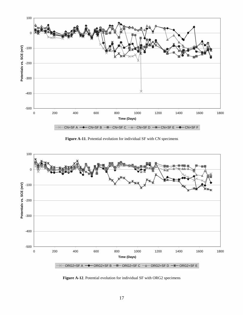
Figure A-11. Potential evolution for individual SF with CN specimens

Figure A-12. Potential evolution for individual SF with ORG2 specimens

-500

-400

-300

-200

-100

0

100

0 200 400 600 800 1000 1200 1400 1600 1800

Time (Days)

Po

ten

tial

s vs

. SC

E (

mV

)

CN+SF A CN+SF B CN+SF C CN+SF D CN+SF E CN+SF F

-500

-400

-300

-200

-100

0

100

0 200 400 600 800 1000 1200 1400 1600 1800

Time (Days)

Po

ten

tial

s vs

. SC

E (

mV

)

ORG2+SF A ORG2+SF B ORG2+SF C ORG2+SF D ORG2+SF E