Embed Size (px)
Citation preview

Paper Number: 300494
History of Science and Statistical Education: Examples from Fisherian and Pearsonian schools
Paper presented at the 2004 Joint Statistical Meeting, Toronto, Canada
Chong Ho Yu, Ph.D.
Website: http://www.creative-wisdom/pub/pub.html
Abstract
Many students share a popular misconception that statistics is a subject-free methodology
derived from invariant and timeless mathematical axioms. It is proposed that statistical
education should include the aspect of history/philosophy of science. This article will
discuss how statistical methods developed by Karl Pearson and R. A. Fisher are driven by
biological themes and philosophical presumptions. Pearson was pre-occupied with
between-group speciation and thus his statistical methods, such as the Chi-squared test, are
categorical in nature. On the other hand, variation within species plays a central role in
Fisher’s framework, and therefore, Fisher’s approach, such as partitioning variance, is
concerned with interval-scaled data. In addition, Fisher adopted a philosophy of embracing
causal inferences and theoretical entities, such as infinite population and gene, while
Pearson disregarded unobservable and insisted upon description of the data at hand. These
differences lead to the subsequent divergence of two hypothesis testing methods, developed
by R. A. Fisher and Neyman/E .S. Pearson, son of Karl Pearson, respectively. Students will
appreciate the meanings of Fisherian and Pearsonian methods if they are exposed to history
and philosophy of science.
R. A. Fisher and Karl Pearson are considered the two most important figures in statistics as well as
influential scholars in evolutionary biology and genetics. While statistical procedures are widely applied by
scholars in various disciplines, including the natural and social sciences, statistics is mistakenly regarded as

Fisher and Pearson 2
a subject-neutral methodology. It is important to point out that as R. A. Fisher and Karl Pearson developed
their statistical schools, both of them were also pre-occupied with biological issues. Nonetheless, some
authors have shifted the focus of Fisher- Pearson dispute from biology to statistical methodology or
philosophy. Morrison (2002) represents the methodology focus by arguing that philosophy such as
Pearson’s positivism did not play an active role in the debate between Mendelism and biometry; rather to
Pearson “the problem of evolution is a problem of statistics” (p.47). In contrast, while discussing the
difference between Fisher and Pearson with regard to Fisher’s synthesis of Mendelism and biometrics,
Norton and E. S. Pearson (1976), the son of Karl Pearson, argued that “their common stated objection was
largely philosophical” (p.153). Nonetheless, Norton’s framework of analysis (1975) emphasizes the
interplay between Pearsonian research on heredity and his philosophy of science.
The complexity of the Fisherian and Pearsonian views might not be adequately approached from a
biological, statistical, or philosophical perspective alone. It is important to point out that both Fisher and
Pearson were practitioners, not pure mathematicians conducting research on self-contained mathematical
systems. In addition, Pearson was versed in German cultural and philosophical studies (Pearson, 1938;
Williams et al., 2003). Therefore, it is plausible that the development of their statistical methodologies
resulted from their philosophical orientations toward biology. Indeed, contemplation of biology issues
played a crucial role in shaping their philosophy of science, and their philosophy of science influenced their
statistical modeling. It is not intention of this article to portray a simplistic view that the influences occur in
a linear fashion–biology-philosophy-statistics. Instead, it could be conceived as an iterative process in
which biology, philosophy and statistics are interwoven. One may argue that their Pearson’s and Fisher’s
philosophies are an abstraction of their statistical practice. On the other hand, one could also analyze
Fisher’s and Pearson’s views on biology by tracing the sources of influence back to statistics. The order of
“biology-philosophy-statistics” taken by this article is merely for the ease of illustration.
In the following section brief background information, such as the influence of biology on both Fisher
and Pearson, the debate between the Schools of Mendelism and Biometrics and the social agenda of
Eugenics, will be introduced. Next, it will discuss the relationship between biology and philosophy of

Fisher and Pearson 3
science in both Fisherian and Pearsonian schools. The thesis is that Pearson is pre-occupied with
between-group speciation and thus his statistical methods, such as the Chi-squared test, are categorical in
nature. On the other hand, variation within species plays a central role in Fisher’s framework and thus
Fisher’s approach, such as partitioning variance, is more quantitative than Pearson’s in terms of the
measurement scale. In addition, Fisher adopted a philosophy of embracing causal inferences and theoretical
entities, such as infinite population and gene, while Pearson disregarded unobservable and insisted upon
description of the data at hand. Afterwards, it will illustrate how Fisher disagreed with Pearson in almost
every aspect of Pearson’s contributions to statistics due to their differences in biology and philosophy. The
last part is an attempt to examine the difference between the significance testing approach developed by
Fisher and the hypothesis testing approach advocated by Neyman and E. S. Pearson, who were both
influenced by Karl Pearson.
Influence of Biology on Fisher and Pearson
Pearson and biology
Karl Pearson was a follower of Galton, who is credited as the founder of the biometric school.
However, Galton’s mathematical approach to biology is coarse; it is Pearson who elevated the statistical
approach to biology to a higher level. Thanks to Galton’s efforts, in the late 18th century it became
commonplace to picture the range of variation of species by a frequency distribution, especially the use of a
normal curve. When Galton attempted to find out what happened to the curve if selection affects a
population over several generations, he proposed the law of ancestral inheritance. Later Pearson followed up
this theme and revised the law of ancestral inheritance with sophisticated statistics (Bowler, 1989).
Besides Galton, the closest colleague of Karl Pearson, W. F. R. Weldon, is also a biologist. Darwinism
occupied a central theme in Weldon’s research. Collaboration between Pearson and Weldon, needless to
say, centered around biological topics. Karl Pearson’s interest in biology was manifested in his speeches
delivered in the Gresham Lectures from 1891 to 1894. Among those thirty-eight lectures, eight of them are
concerned with philosophy of science, and later these papers were revised and published in a book entitled
The grammar of science. The rest of the lectures are mostly related to biology. Eighteen of those papers

Fisher and Pearson 4
were named “Mathematical Contribution to the Theory of Evolution” with different subtitles. In these
papers Pearson introduced numerous concepts and procedures that have great impact on quantitative
methodology, such as standard error of estimate, use of histograms for numeric illustration, and use of
determinantal matrix algebra for biometrical methods. One of Pearson’s goals was to develop a
mathematical approach to biology. When Pearson started to develop the idea of speciation in terms of
asymmetrical distributions, he proudly proclaimed, “For the first time in the history of biology, there was a
chance of the science of life becoming an exact, mathematical science” (cited in Magnello, 1996, p.59). In
some lectures Karl Pearson focused on the research agenda of Weldon. To be specific, Pearson and Weldon
needed a criterion to reconstruct the concept of species. This provided the impetus to Pearson’s statistical
innovation of the Chi-square test of goodness of fit in 1892 (Magnello, 1996). No wonder Magnello (1996)
bluntly asserted that “Pearson’s statistical innovation was driven by the engine of evolutionary biology
fuelled by Weldon” (p. 63).
Fisher and biology
The influences of biology on Fisher could be traced back to as early as Fisher’s primary and secondary
schooling. According to Joan Fisher-Box (1978), daughter of R. A. Fisher, Fisher excelled at school in
biological and physical science as well as mathematics. Some of the books he chose as school prizes, such as
his choice of the complete works of Charles Darwin in 1909, indicate his early interest in biology. At that
time Fisher read many heavy-duty books on biology such as A familiar history of birds, Natural history and
antiquities of Selnorne, “Introduction to zoology, and Jelly-fish, starfish, and sea-urchins Later when Fisher
went to Cambridge University, he read three newly published books on evolution and genetics by the
Cambridge University Press.
It is a well-known fact that Fisher’s 1918 paper on the synthesis of Mendelism and biometrics is
considered a milestone in both biology and statistics. Actually, in 1911 Fisher had contemplated this
synthesis in an unpublished paper, which was a speech delivered to the Cambridge University’s Eugenics
Society. At that time biological science was not fully conceptualized in a quantitative manner. In the 1911
paper, Fisher started to recognize the importance of quantitative characters to biological studies. It is also

Fisher and Pearson 5
noteworthy that during Fisher’s study at Cambridge, Bateson, a Professor of Biology who specialized in
genetics, gave Fisher tremendous influences. To Bateson the origin of species is equated to the origin of
gradual variation. Henceforth, variation has become a major thread of Fisherian thought. However, in the
1911 paper Fisher departed from Bateson’s gradualism and suggested a thorough quantitative study of
variation in both Mendelian and Darwinian senses (Bennett, 1983).
From 1915 for about twenty years, Fisher maintained extensive contact with Leonard Darwin, son of
Charles Darwin. During much of this time they corresponded with each other one another every few days.
Leonard Darwin introduced Fisher to a job in the Eugenics Education Society and encouraged him to pursue
biological research topics. In 1916 when one of Fisher’s papers was rejected by the Royal Society due to
negative comments made by Karl Pearson, Leonard Darwin financed Fisher so that Fisher could pay another
journal for printing the paper. That paper, which appeared in 1918, is the one that synthesizes Mendelism
and biometrics (Norton, 1983). In exchanging ideas on academic topics, Darwin repeatedly encouraged
Fisher to develop a mathematical approach to evolution and genetics. This invitation was well received by
Fisher (Bennett, 1983). Indeed, Fisher observed this methodological “gap” in biological scholarship. In
1921 when Fisher reviewed the paper entitled “The relative value of the processes causing evolution,” he
commented, “The authors evidently lack the statistical knowledge necessary for the adequate treatment”
(cited in Bennett, 1983, p. 11). Throughout his career, Fisher continuously devoted tremendous effort to
developing statistical methods for evolution and genetics. Fisher’s 1958 book entitled The genetical theory
of natural selection summarizes his statistical contribution to biology. In brief, it is obvious that the
development of Fisherian statistical methodology was driven by his motivation to fill the methodological
gap in biological science.
Background of the debate between R. A. Fisher and Karl Pearson
In the late 19th century, Charles Darwin proposed natural selection, in terms of survival for the fittest, as
a driving force of evolution. Francis Galton, a cousin of Darwin, was skeptical of the selection thesis. Galton
discovered a statistical phenomenon called regression to the mean, which is the precursor of regression
analysis. According to regression to the mean, in a population whose general trait remains constant over a

Fisher and Pearson 6
period of generations, each trait exhibits some small changes. However, this change does not go on forever
and eventually the traits of offspring would approximate those of the ancestors. For example, although we
expect that tall parents give birth to tall children, we will not see a super-race consisting of giants after ten
generations, because the height of offspring from tall people would gradually regress towards the mean
height of the population. According to Darwinism, small improvement in a trait happens across generations,
and natural selection, by keeping this enhanced trait, makes evolution possible, but Galton argued that the
regression effect counter-balances the selection effect (Gillham, 2001).
The central question of evolution is whether variation of a trait is inheritable. In the late 19th century
Mendel gave a definite answer by introducing an elementary form of genetic theory. Mendel’s theory was
forgotten for a long while but it was re-discovered by de Vries in 1900. In contrast to Darwin’s position that
evolution is a result of accumulated small changes in traits, biologists who supported Mendel’s genetics
suggested otherwise: evolution is driven by mutation and thus evolution is discontinuous in nature. By the
early 20th century, two opposing schools of thought had developed, namely, biometricians, who supported
discontinuous evolution with “sports,”and Mendelians, who supported continuous evolution with gradual
changes. Although Galton rejected the idea of small changes in traits as an evolutionary force, he was
credited as the pioneer of biometrics for his contribution of statistical methods to the topic of biological
evolution.
Another important piece of background information is the fashion of Eugenics during the late 19th
century and early 20th century. During that period of time many research endeavors were devoted to
explaining why Western civilizations were superior to others (e.g., research on intelligence) and how they
could preserve their advanced civilizations. According to Darwinism, the fittest species are the strongest
ones who could reproduce more descendants. This notion fit the social atmosphere very well, since
Darwinism could rationalize the idea that the West is stronger and thus fitter; it has the “mandate destiny”
because the nature has selected the superior. Both Fisher and Pearson attempted to provide an answer to a
question that was seriously concerned by Western policy makers and scholars. Under the
Mendelian-Darwinian-Biometrician synthesis, Fisher suggested that the only way to ensure improvement of

Fisher and Pearson 7
the nation was to increase the reproduction of high-quality people (Brenner-Golomb, 1993; Gigerenzer et al,
1989).
Biology and philosophy of science in Pearsonian school
Grammar of science
Classification of facts. In 1892 Karl Pearson published a book entitled The grammar of science, which
manifested his positivist view on science. In Pearson’s view scientific methodology is a “classification of
facts” (p.21), and thus causal inferences and explanations are unwarranted. In this book Pearson paid much
attention to evolutionary biology, in which “variation,” “inheritance,” “natural selection,” and “sexual
selection” were treated as mere description. It may be difficult to determine whether his biological thought
influenced his philosophy of science or vice versa. In The grammar of science, Pearson declared that his
proposed scientific method is subject-free by saying, “The unity of all science consists alone in its method,
not in its material…it is not the fact themselves which form science, but the method in which they are dealt
with” (p.16).
Nevertheless, in spite of this claim of “subject-free” methodology, there is an interesting link between
the notion of speciation in biology and the notion of science as a classification of facts. Speciation is an
evolutionary formation of new biological species, usually by the division of a single species into two or
more genetically distinct ones. In later years Pearson employed statistics to divide a non-normal distribution
into two normal distributions as a means to describe speciation (Magnello, 1996). In addition, one of the
major contributions to statistics by Pearson is the invention of the Chi-squared test, which is a test of
goodness of fit using discrete and categorical data. In The Grammar of Science Pearson strongly
disapproved of metaphysics, German Hegelianism, and religion for their ambiguity and unanswerable
questions. Interestingly enough, rather than promoting science as a methodology of using precise
continuous-scaled measurement with ten decimal points following each numeric output, Pearson regarded
science as a discrete classification of facts, which fits well with speciation in biology.
Anti-theoretical entity and anti-cause. Pearson’s positivist attitude could also be found in his position
on anti-theoretical entities. In the first edition of The grammar of science (1892/1937), Karl Pearson mocked

Fisher and Pearson 8
the theory of atoms. After 1900 the impetus for Mendelian genetics had been revived. However, as late as
1911, Pearson still showed no interest in unobservable entities by asserting, in the Preface to the third
edition of The grammar of science, that theoretical entities are nothing more than constructs for
conveniently describing our experience. Causal explanations, equally hidden and unobservable, were also
dissatisfying to Pearson. In the third edition of “The Grammar of Science,” he added a new chapter entitled
“Contingency and Correlation—the Insufficiency of Causation.” Pearson strongly objected to using hidden
causal forces as an explanation in science. Instead, he proposed using a contingency table, which is a
description and classification of data. His anti-cause position is obviously influenced by Galton’s
correlational method. In 1889 Pearson wrote, “It was Galton who first freed me from the prejudice that
sound mathematics could only be applied to natural phenomena under the category of causation” (cited in
Pearson, 1938, p.19). Interestingly enough, this anti-cause position is also tied to his crusade against
animistic philosophy, such as employing “teleology” and “will,” in biology (Pearl, 2000). When Darwinism
was proposed as a naturalistic explanation of the origin and evolution of species, the causal mechanism
behind evolution was portrayed in the fashion that species are “willing” to evolve towards a teleological
consummation. As a scholar who disliked metaphysics and the Hegelian notion that history evolves with an
ideal, it is not surprising that Pearson was opposed to casual explanations in biology and favored
contingency tables.
Nonetheless, Porter (2004) argued that the position of downplaying invisible, hypothetical objects did
not play a central role in Pearson’s rejection of Mendelian genetics. He was critical of concepts such as
“force” and “matter,” but not “gene” and “molecule.” Rather he charged that the Mendelians defined nature
in one and only one approach while indeed natural phenomena could be described in multiple ways. In
philosophy of science terminology, there should be more than one way to “save the phenomenon.”
The Grammar of science was warmly embraced by Pearson’s scholarly contemporaries such as
Neyman, who later co-developed the Neyman/Pearson hypothesis testing approach with Karl Pearson’s son,
E. S. Pearson. Neyman said, “We were a group of young men who had lost our belief in Orthodox religion,
not from any sort of reasoning, but because of the stupidity of our priests, [But] we were not freed from

Fisher and Pearson 9
dogmatism and were prepared in fact to believe in authority, so far as it was not religious. The reading of
The Grammar of Science…was striking because…it attacked in an uncompromising manner all sorts of
authorities….At the first reading it was this aspect that struck us. What could it mean? We had been unused
to this tone in any scientific book. Was the work ‘de la blague’ [something of a hoax] and the author a
‘canaille’ [scoundrel] on a grand scale…? But our teacher, Bernstein, had recommended the book; we must
read it again” (cited in Reid. 1982, pp. 23-24).
Pearsonian school of statistics
Pearsonian methodologies carry unmistakable marks of his philosophy of science. Karl Pearson made
four major contributions to statistical methods before the turn of the century: (1) Method of moments
(Pearson, 1894), (2) Curve fitting based on least squares (Pearson, 1895), (3) Correlation (Pearson & Filon,
1898), and (4) Chi-squared test of goodness of fit (Pearson, 1900). These methodologies share two common
threads, namely, correlation instead of causation, and description of data at hand instead of idealistic,
theoretical modeling.
Method of moments. In 1893-94 Karl Pearson wrote a paper in response to Weldon’s request about
speciation in terms of breaking up a distribution into two. In this paper Pearson introduced the method of
moments as a means of fitting a curve to the data (Pearson, 1928; Magnello, 1996). To be specific, the
method of moments was applied to the estimation of a mixture of normal distributions. In a normal
distribution, which is symmetrical in shape, only the first and second moments (mean and standard
deviation) are matters of concern. In a non-normal distribution, the third and fourth moments (skewness and
kurtosis) are essential for describing the distribution. Although Galton is arguably the first scholar to employ
statistics in biology, he was so obsessed with normal distributions that he spent his whole life attempting to
fit any data to a normal curve. In contrast, Pearson found that symmetrical normality is by no means a
universal phenomenon, especially for problems in evolutionary biology. As a remedy, Pearson introduced
the method of moments as a statistical approach of curving fitting for both symmetrical and asymmetrical
distributions. To be specific, a bi-modal distribution, also know as a double-humped curve, could be

Fisher and Pearson 10
dissected into two normal curves. Its application is to break up a species into two species. When the measure
of a trait of a species appears to be non-normally distributed, speciation has occurred.
Least square and curve-fitting. The least square method and curve-fitting are built upon the theory of
error. When multiple measures were administered in astronomy research , there were always some
fluctuations. In the past scientists had tended to dismiss certain unreliable measurements, but later scientists
took the average of multiple measures. In this approach, the degrees of the departure from the mean are
regarded as errors or residuals. To Pearson the aim of curve-fitting is to minimize the residuals or errors. It is
important to point out that this approach is more data-driven than model-driven since it is obvious that errors
varying from sample to sample are taken into account. Today the theory of error is in line with the residual
analysis that is commonly seen in the school of Exploratory Data Analysis (EDA), since EDA is also more
data-driven than model based (Behrens & Yu, 2003).
In addition, curve-fitting as a graphical technique is tied to Pearson’s emphasis on the descriptive
nature of scientific methodology. During the 1880s Pearson concentrated on graphical methods as his
central contributions to engineering education. Later he extended his vision to biometrics, in which the
geometrical sense of evolutionary processes was said to be detectable by graphing methods. To be specific,
he thought that he could find the effects of natural selection from frequency curves. However, unlike data
visualization techniques in modern EDA, Pearson was opposed to curve smoothing because it might blend
away double peaks of correlation surfaces (Porter, 2004).
Correlation. Galton invented the concept of correlation and Pearson further expanded this idea by
introducing several correlation coefficients such as Product Moment and tetrachoric, as a replacement for
causal inferences. In Pearson’s view, the ultimate essence of biological knowledge is statistical and there is
no room for causal factors. To be specific, if variables A and B are correlated, it does not necessarily imply
that A causes B or vice versa. For example, the correlation coefficient derived from a bivariate distribution
fitted to the heights of fathers and sons could be used to describe the process of heredity, but one should not
specify any biological mechanism in a causal sense. This approach has been applied by both Karl Pearson
and W. F. R. Weldon in biological research, but Pearson even went further to use correlation to reject

Fisher and Pearson 11
Mendelism. By computing the correlation coefficients of physical traits among relatives sampled from
human populations, Pearson concluded that there is no evidence that the variance of height among humans
could be explained by heredity, and thus the correlational studies contradicted the Mendelian scheme of
inheritance (Norton, 1975; Provine, 2001).
Chi-squared. Chi-squared is a test of goodness of fit between the expected and the observed frequency
of categorical data in a contingency table. E. S. Pearson (1938), son of Karl Pearson, praised the
Chi-squared test as “a powerful new weapon in the hands of one who sought to battle with the myths of a
dogmatic world” (p.31). Pearson presented the Chi-squared distribution in place of the normal distribution
to solve the goodness of fit for multinomial distributions. In Pearson's view, there is no “true” chi-square in
the Platonic or absolute sense, or the so-called “true” chi-square cannot be estimated even if it exists. The
focal point of the Chi-squared test is the exact frequency of the data and thus there is no probabilistic
property in the data. To be specific, for Pearson the so-called probabilities associated with the test do not
represent a model-based attribute such as the frequency of incorrectly rejecting the hypothesis. Rather, it is
just a convenient way to describe the fit between the hypothesis and the data (Baird, 1983). Like the modern
Rasch modeling school, Pearson emphasized that the model must fit the data, but not the other way around.
When data seemed to contradict calculation, he doubted the mathematics (Porter, 2004).
Biology and philosophy of science in the Fisherian school
Mendelian genetics and Model-based deduction
Unlike Pearson, Fisher did not write any book concerning philosophy of science. In the collected
correspondence of Fisher edited by J H. Bennett (1990), only eight pages of Fisher’s writing are put under
the category of “history and philosophy of science.” Moreover, most of these writings are fragmented
thoughts rather than systematic inquiry into the history and philosophy of science. Nevertheless, Fisher’s
philosophical ideas are manifested in his view on biology. Neyman’s praise of Pearson, as cited above,
indicates the academic atmosphere of the late 19th century. Being skeptical of metaphysics and religion,
certain scholars were eager to search for methodologies of high certainty and low ambiguity. To Fisher,
Mendelian genetics was a viable means because genetics could potentially explain a large amount of
Fisher and Pearson 12
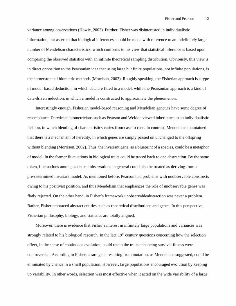
variance among observations (Howie, 2002). Further, Fisher was disinterested in individualistic
information, but asserted that biological inferences should be made with reference to an indefinitely large
number of Mendelism characteristics, which conforms to his view that statistical inference is based upon
comparing the observed statistics with an infinite theoretical sampling distribution. Obviously, this view is
in direct opposition to the Pearsonian idea that using large but finite populations, not infinite populations, is
the cornerstone of biometric methods (Morrison, 2002). Roughly speaking, the Fisherian approach is a type
of model-based deduction, in which data are fitted to a model, while the Pearsonian approach is a kind of
data-driven induction, in which a model is constructed to approximate the phenomenon.
Interestingly enough, Fisherian model-based reasoning and Mendelian genetics have some degree of
resemblance. Darwinian biometricians such as Pearson and Weldon viewed inheritance in an individualistic
fashion, in which blending of characteristics varies from case to case. In contrast, Mendelians maintained
that there is a mechanism of heredity, in which genes are simply passed on unchanged to the offspring
without blending (Morrison, 2002). Thus, the invariant gene, as a blueprint of a species, could be a metaphor
of model. In the former fluctuations in biological traits could be traced back to one abstraction. By the same
token, fluctuations among statistical observations in general could also be treated as deriving from a
pre-determined invariant model. As mentioned before, Pearson had problems with unobservable constructs
owing to his positivist position, and thus Mendelism that emphasizes the role of unobservable genes was
flatly rejected. On the other hand, in Fisher’s framework unobservableabstraction was never a problem.
Rather, Fisher embraced abstract entities such as theoretical distributions and genes. In this perspective,
Fisherian philosophy, biology, and statistics are totally aligned.
Moreover, there is evidence that Fisher’s interest in infinitely large populations and variances was
strongly related to his biological research. In the late 19th century questions concerning how the selection
effect, in the sense of continuous evolution, could retain the traits enhancing survival fitness were
controversial. According to Fisher, a rare gene resulting from mutation, as Mendelians suggested, could be
eliminated by chance in a small population. However, large populations encouraged evolution by keeping
up variability. In other words, selection was most effective when it acted on the wide variability of a large

Fisher and Pearson 13
population. This proposal addressed the question of evolution in a continuous and unbranching line. In
contrast to Pearson, Fisher ignored the issue of speciation, splitting of a population into several discrete and
distinct branches (Bowler, 1983). Fisher’s attempt to theorize selection in terms of “infinitely large
populations” clearly demonstrates a link between his research agenda in biology and his later development
of statistical inference based upon infinite, theoretical distributions, which will be discussed in a later
section. Also, the theme of seeking support for continuous evolution sheds some light on Fisher’s
orientation towards quantitative thinking in a continuous scale, as opposed to Pearson’s discrete thinking,
such as the Chi-squared test and the classification of facts.
Fisherian school of statistics
It is not exaggerating to say that Fisher’s career, to a certain extent, was built upon his opposition to
Pearsonian ideas. Fisher’s first paper, “On the absolute criterion for fitting frequency curves” (1912), is
considered a rebuttal of Pearson’s least squares and curve fitting. The clash between the two giants came to
a crescendo in 1918 when Fisher partitioned variances (the precursor of Analysis of Variance) to synthesize
Mendelism and Biometry, and hence rejected the Pearsonian idea that Mendelism is incompatible with
evolution. But the battle didn’t end here. In 1922 Fisher proposed a change in the degree of freedom of the
Chi-squared test introduced by Pearson in 1900. Fisher’s contributions to statistics and biology go beyond
the development of preceding theories, but in terms of confronting Pearsonian notions, his ideas could be
summarized as the following: (1) Maximum likelihood estimation as an opposition to least squares; (2)
Analysis of variance as an opposition to a-causal description; (3) Modification of Pearsonian Chi-Squared.
Each of the above will be discussed below.
Maximum likelihood. Aldrich (1997) asserted that Fisher’s 1912 paper is a “very implicit piece of
writing, and to make any of it explicit, we have to read outside and guess” (p.162). In Aldrich’s view,
although Fisher did not mention Pearson in that paper, the paper reads like a critique of Pearson’s theory of
curve fitting. In the paper Fisher proposed using the scale-independent absolute criterion as a replacement
for the theory of error and the least squared because of their shortcoming in scale-dependence. Later, during
Fisher’s dispute with Bayesians such as Jeffrey, Fisher further expanded the idea of absolute criterion and

Fisher and Pearson 14
eventually developed the maximum likelihood estimation. By applying the maximum likelihood function to
gene frequency and recombination frequency estimation, biologists overcame the problems of multiple
factors in biology (Piegorsch, 1990).
The main point is that statistical methods could not be confined by individual data sets, whose
properties vary from time to time, from place to place, and from person to person; probability should carry
objective and invariant properties that can be derived from mathematics. As a competent mathematician,
Fisher constructed three criteria for desirable properties of estimators to the unknown population, namely,
unbiasedness, consistency, and efficiency (Eliason, 1993). A detailed mathematical demonstration of these
properties is beyond the scope of this paper; nevertheless, the following brief description of Fisher’s
approach demonstrates how Fisher elegantly constructed an objective approach to statistics and probability
that is effective even if the hypothetical population is unknown in distribution and infinite in size.
Figure 1. Unbiased estimator.
In Figure 1, the bell-shaped curve denotes the hypothetical distribution. The red line represents the
population parameter while the yellow line represents the estimation. If the estimated parameter is the same
as the true parameter, this estimation is considered unbiased. However, an estimator has variance or

Fisher and Pearson 15
dispersion. In Figure 1 the green line with arrows at both ends indicates that the estimator may fall
somewhere along the dispersion. The efficient estimator is the one that has achieved the lowest possible
variance among all other estimators, and thus it is the most precise one. Moreover, the goodness of the
estimation is also tied to the sample size. As the sample size increases, the difference between the estimated
and the true parameters should be smaller and smaller. If this criterion is fulfilled, this estimator is said to be
consistent. Hence, researchers can make probabilistic inferences to hypothetical populations using these
objective criteria. Today some statisticians believe that if the likelihood approach serves as the sole basis for
inference, analyzing residuals of data is unnecessary (Nerlove, 1999).
Analysis of variance. In 1916 Karl Pearson, who served as a reviewer of the Journal of Royal Society,
rejected a paper submitted by Fisher regarding Mendelism and Darwinism. Fisher blamed the rejection on
the paper being sent to Pearson, “a mathematician who knew no biology,” and another reviewer, a biologist
lacking mathematical knowledge (cited in Morrison, 2002). Two years later, with Leonard Darwin’s
financial assistance, Fisher paid the Transactions of the Royal Society of Edinburgh to publish that paper. In
that paper Fisher (1918) bluntly rejected Pearson’s assertion that biometrics had denied Mendelism. Based
on the same data set collected by Pearson for denying Mendelism, Fisher demonstrated that the hypothesis
of cumulative Mendelian factors seems to fit the data very well. By re-formulating statistical procedures and
probabilistic inferences, Fisher concluded that heritable changes in the Mendelian sense could be very small
and evolution in the Darwinian sense could be very slow, and these subtle differences could be detected by
Fisher’s version of biometrics.
Fisher’s 1918 paper is highly regarded as a milestone in both statistics and biology for the introduction
of the prototype of Analysis of Variance as well as the synthesis of Mendelism, biometry and evolution
(Morran & Smith, 1966). More importantly, it carries important implications for philosophy of science. As
mentioned before, Pearson frequently employed descriptive statistics such as correlation coefficients rather
than causal inferences. However, in Fisher’s methodology variance of traits is partitioned and therefore it is
possible to trace how much variance of a variable is accounted for by the variance of another. Aldrich (1995)
praised Fisher’s 1918 paper as “the most ambitious piece of scientific inference” (p. 373). Aldrich cited

Fisher and Pearson 16
Koopmans and Reiersol (1950) and Cox (1958) to distinguish statistical inference from scientific inference.
The former deals with inference from sample to population, while the latter addresses the interpretation of
the population in terms of a theoretical structure. This is no doubt revolutionary because Fisher went beyond
correlation to causation, beyond description to explanation, and beyond individual observations to
theoretical structure.
It is noteworthy that in the 1918 paper Fisher coined the term “variance” as a means to partition
heritable and non-heritable components of species. It is generally agreed that the concept of “variance”
revolutionized modern statistical thinking. To be specific, not only are Analysis of Variance and its
extended methods, such as Analysis of Covariance (ANCOVA) and Multiple Analysis of Variance
(MANOVA), based upon the concept of “variance,” but correlational and regression analysis can also be
construed in terms of “variance explained” (Keppel & Zedeck, 1989). In addition, in Psychometrics
reliability is also conceived as a relationship between the true score variance and the error variance by
followers of the True Score Theory (Yu, 2001).
Modified Chi-squared test. Pearson invented the Chi-squared test as a specific materialization of the
notion that science is a classification of facts. Fisher was not opposed to the use of Chi-squared; he applied
this to expose the errors made by Gregor Mendel, the father of genetics (Press & Tanur, 2001; Fisher, 1936).
Mendel established the notion that physical properties of species are subject to heredity. In accumulating
evidence for his views, Mendel conducted a fertilization experiment in which he followed several
generations of axial and terminal flowers to observe how specific genes were carried from one generation to
another. However, upon subsequent examination of the data using Chi-squared tests of association, Fisher
(1936) found that Mendel's results were so close to the predicted model that residuals of the size reported
would be expected by chance less than once in 10,000 times if the model were true.
The clash between Fisher and Pearson on Chi-squared happened in 1922 when Fisher introduced
“degrees of freedom” to modify the meaning of Chi-squared. Fisher argued that in terms of causal
explanation every free parameter reduces one degree of freedom. Pearson, as the inventor of the test, was
opposed to Fisher’s suggestion (Baird, 1983). In contrast, Fisher’s criticism was well-taken by Yule and

Fisher and Pearson 17
Greenwood. They attributed Pearson’s stubbornness to his personality, an unwillingness to admit errors. But
Porter argued that perhaps there is also something in Pearson’s attitude that reflects a long standing ideal of
curve-fitting, the notion of data over model (Porter, 2004).
Obviously, Pearson was on the wrong side of history. Chi-squared is now applied as Fisher argued it
ought to be (Baird, 1983). The degree of freedom, by definition, is the number of pieces of useful
information, which is determined by the sample size and also the number of parameters to be estimated (Yu,
Lo, & Stockford, 2001). In other words, the degree of freedom is a measure of the informativeness of a
hypothesis. Using Chi-squared alone as a measure of fit suffers from a drawback: Chi-squared statistics is a
function of sample size. As a remedy today for detecting misfits in Item Response Theory, it is a common
practice to divide the Chi-squared by degrees of freedom (Chi-sq/df).
More importantly, Fisher’s interpretation of Chi-squared represents a very different philosophy from
Pearson’s. As mentioned before Pearson did not accept the notion of true Chi-Squared; the meaning of “fit”
between the expected and the observed, to him, was nothing more than constructing a convenient model to
approximate the observed frequencies in different cells of a contingency table. However, to Fisher a true
Chi-squared could be obtained even when expected cell frequencies must be estimated. In this sense, the
meaning of “fit” is the closeness to the truth of a hypothesis (Baird, 1983).
Comparison between Fisherian and Pearsonian statistics indicates that Fisher favored statistical
thinking in terms of variance on a continuum while Pearson oriented towards statistical thinking in a
discrete mode. Actually their differences go beyond this. As mentioned before, Pearsonian methodology is
tied to his philosophy of science, which is a-causal and descriptive in essence. Fisher realized that this
reasoning was a hindrance to biological science because to him scientists must contemplate a wider domain
than the actual observations. To Fisher the concept of variation or variance is not confined to actual cases,
but also theoretical distributions including a wider variation that has no mapping to the empirical world. For
instance, biologists would take the existing two sexes for granted; no biologist would be interested in
modeling what organisms might experience if there were three or more sexes. However, from a
mathematical viewpoint it is logical to consider this question with reference to a system of possibilities
Fisher and Pearson 18
infinitely wider than the actual (Fisher-Box, 1978). Today philosophers call this type of reasoning
“counterfactual.” Counterfactual reasoning of possible worlds lead Fisherians to go beyond mere
description of the actual world.
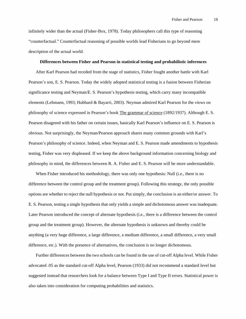
Differences between Fisher and Pearson in statistical testing and probabilistic inferences
After Karl Pearson had receded from the stage of statistics, Fisher fought another battle with Karl
Pearson’s son, E. S. Pearson. Today the widely adopted statistical testing is a fusion between Fisherian
significance testing and Neyman/E. S. Pearson’s hypothesis testing, which carry many incompatible
elements (Lehmann, 1993; Hubbard & Bayarri, 2003). Neyman admired Karl Pearson for the views on
philosophy of science expressed in Pearson’s book The grammar of science (1892/1937). Although E. S.
Pearson disagreed with his father on certain issues, basically Karl Pearson’s influence on E. S. Pearson is
obvious. Not surprisingly, the Neyman/Pearson approach shares many common grounds with Karl’s
Pearson’s philosophy of science. Indeed, when Neyman and E. S. Pearson made amendments to hypothesis
testing, Fisher was very displeased. If we keep the above background information concerning biology and
philosophy in mind, the differences between R. A. Fisher and E. S. Pearson will be more understandable.
When Fisher introduced his methodology, there was only one hypothesis: Null (i.e., there is no
difference between the control group and the treatment group). Following this strategy, the only possible
options are whether to reject the null hypothesis or not. Put simply, the conclusion is an either/or answer. To
E. S. Pearson, testing a single hypothesis that only yields a simple and dichotomous answer was inadequate.
Later Pearson introduced the concept of alternate hypothesis (i.e., there is a difference between the control
group and the treatment group). However, the alternate hypothesis is unknown and thereby could be
anything (a very huge difference, a large difference, a medium difference, a small difference, a very small
difference, etc.). With the presence of alternatives, the conclusion is no longer dichotomous.
Further differences between the two schools can be found in the use of cut-off Alpha level. While Fisher
advocated .05 as the standard cut-off Alpha level, Pearson (1933) did not recommend a standard level but
suggested instead that researchers look for a balance between Type I and Type II errors. Statistical power is
also taken into consideration for computing probabilities and statistics.

Fisher and Pearson 19
Figure 2. Fusion of Fisher and Pearson models
Fisherian model
In Figure 2, the y-axis is the frequency and the x-axis is the standardized score with the mean as zero and
the standard deviation as one. The curve on the left hand side is the null distribution introduced by Fisher. It
is important to note that this is the sampling distribution, which appears in theory only. It is derived from
neither the population nor the sample. In theory, if there is no difference between the control and treatment
groups in the population, the subtraction result is zero. However, there are always some sampling
fluctuations due to measurement errors and other factors. In a thought experiment, if many samples are
drawn from the same population, the difference is not exactly zero all the time. On some occasions it is
above zero, and in some cases it is below zero. According to the Central Limit Theorem, when these scores
are plotted, a bell-shaped distribution is formed regardless of the shape of the population distribution (Yu,
Anthony, & Behrens, 1995). In the Fisherian methodology, a pre-determined Alpha level (red line) is set to
guide the researcher in making a judgment about the observed sample. After the statistical attributes of the
observed sample are found, the sample is compared against this theoretical sampling distribution. If the
sample is located in the right hand side of the Alpha level, the data are said to be extremely rare, and thus the
null hypothesis is rejected. Therefore, the region in the right hand side of the Alpha level is called the
“region of rejection.”

Fisher and Pearson 20
At first glance, the approach adopted by Fisher seems overly simplistic. Why did Fisher recognize just
one null hypothesis? Why did he want only a dichotomous answer? Given Fisher’s model-based reasoning
and his quest for certainty derived from Mendelian genetics, his use of null hypothesis testing is not
surprising.
Neyman/Pearson model
Neyman and E. S. Pearson enriched the methodology by introducing the concepts of alternate
hypothesis, power, and Type I and Type II errors (Beta). According to Neyman and E. S. Pearson, it is not
helpful to conclude that either there is no difference or some difference. If the null hypothesis is false, what
is the alternative? The development of Neyman/Pearson’s notion of alternate distributions may be partly
tied to E. S. Pearson’s father’s disagreement with Galton on the nature of biological data. Galton believed
that all biological data are normally distributed and variations should be confined within certain parameters.
As mentioned before, Galton believed in regression to the mean, in which every naturally occurring variable
has a fixed mean and all values of the variable should tend to scatter around the mean. On the other hand,
Karl Pearson (1896) held a more open-ended view of distributions—the world should have more than one
type of distribution. Data could take on a variety of shapes, which could be skewed, asymmetrical, flat,
J-shaped, U-shaped, and many others. Skew distributions and skew variations could occur in cases of
disease and heredity (Magnello, 1996).
Besides providing an alternate hypothesis, Neyman and Pearson also changed the concept of probability
from static and single-faceted to dynamic and multi-faceted. If the difference between the control and the
treatment groups is small, it is possible that the researcher is unable to detect the difference when indeed the
null hypothesis is false. This is called a Type II error, also known as “Beta” or “miss.” On the contrary, the
researcher may also reject the null hypothesis when in fact there is no difference. In this case, the researcher
makes a Type I error, also known as “false alarm.”
Under the frequentist logic of E. S. Pearson, several other probability concepts were introduced: Power,
associated with the alternate hypothesis, is the probability that the null hypothesis is correctly rejected (the
blue area in Figure 2), whereas Beta is the probability of Type II error (the green area). In this dynamic

Fisher and Pearson 21
model, power is a function of sample size, Alpha level, and the supposed mean difference between the two
groups, which is also known as “effect size.”
Why did E. S. Pearson introduce the notions of Type I and Type II errors and power? It seems that these
criteria are tied to specific situations. For example, in a research setting where the sample size is small, the
statistical power is also small, and as a result, Type II error is inflated. In other words, the Fisherian
universal model-based inference is replaced by a type of inference that takes attributes of data sets at hand
into account. Indeed, the idea of power could be traced back to the development of the Chi-Squared test by
Karl Pearson. As mentioned before, Karl Pearson did not view a test of fit as a measure of the closeness of
data to the “truth,” but just as a measure of adequacy of some theoretical mathematical model for the
observed data. To justify this orientation of “fit,” Pearson referred to his test of fit of what we now call the
statistical power. His argument is that with a sufficiently large sample the Chi-squared test can suggest
whether the hypothesized model could describe the data (Inman, 1994). E. S. Pearson and Karl Pearson were
truly in the same vein regarding statistical inferences.
More importantly, E. S. Pearson viewed the interpretation of statistical inference as a purely
behavioristic one that refrained from any epistemic interpretation. Unlike Fisherian deductive inference, in
which the observed is compared against the model to deduce a dichotomous conclusion, Pearsonian
inference was thought to be inductive behavior, not inductive inference (Gigerenzer et al, 1989). The term
“inductive behavior” shows the resemblance between Karl Pearson’s and E. S. Pearson’s thought.
“Induction” indicates that the researcher should focus on collecting individual observations as a basis of
drawing conclusions, whereas “behavior” implies that the conclusion has nothing to do with estimating a
true parameter based on the sample at hand; rather the behavior is an action taken by the researcher based on
the conclusion as if it were true.
Concluding Remarks
By citing the history of Fisher and Pearson, this article attempts to debunk the myth that statistics is a
subject-free methodology derived from invariant and timeless mathematical axioms. As discussed above,
biological themes and philosophical presumptions drove Karl Pearson and R. A. Fisher to develop their

Fisher and Pearson 22
statistical schools. It is fascinating to see that both giants came from the same starting point (developing a
mathematical approach in biology), but eventually went in different directions. This chasm got even wider
when the Fisherian and Pearsonian philosophies were actualized in hypothesis testing. Today, although
many authors realize that current hypothesis testing is a fusion of the Fisher and Pearson/Neyman schools,
few recognize the biological and philosophical elements in the origin of this hybrid model. The following
table summarizes the differences between the Fisherian and Pearsonian schools:
Table 1. Difference between Fisherian and Pearson schools
Fisherian Pearsonian Philosophy Accept causal inference Favor a-causal description Inference based upon theoretical
worlds, such as infinite populations and counterfactual worlds
Inference based on observed data.
Biology Variation is the central theme; ignore speciation
Speciation is the central theme
Synthesize Mendelism and biometrics
Reject Mendelism
Statistics Use the Maximum Likelihood Estimation, which is model-based
Use Method of Moments, theory of error and least squared, which are data-driven
Use variance partitioning Use correlation and regression Use degree of freedom to amend
the Chi-squared test Use Chi-squared test of goodness of fit
Owing to the contributions by Fisher and Pearson, today statistical thinking continues to be a vibrant
component in evolutionary biology. For example, recent scholarship by Walsh (2003) and his colleagues
(2002) demonstrated that natural selection could appeal to the statistical structure of populations and
sampling error. Interestingly enough, Walsh (2003) didn’t view Fisher’s integration of statistics, genetics
and evolution as a successful one, because to Walsh Darwinian selection is environment-based, forceful,
and causal while genetic selection is probabilistic and statistical. Walsh et al. (2002) used the following two
experimental setups to illustrate the difference between a dynamical model based upon driving forces and a
statistical model based on the population structures. In the first experiment a feather is dropped from certain
height. Although the landing location of the feather appears to be random, indeed it could be well-explained

Fisher and Pearson 23
by the gravitational force, wind direction and its speed at a certain time. The so-called probabilistic
explanation of the outcome is just due to our ignorance of those forces. In the second experiment ten coins
are drawn at random out of 1000 coins: half with heads up and head with heads down. In this case, the
expected outcome of the coin is not generated by attending to the forces acting on the coins, but by taking
into account the structure of the population being sampled.
Discussing whether the Fisherian synthesis of Mendelism, Biometry and Evolution is successful in
resolving the difference between a causal and a statistical explanation is beyond the scope of this paper.
Indeed, the issue of whether statistical and causal laws are fundamentally different is philosophical in nature
(Glymour, 1997). Nonetheless, this example illustrates how biology, philosophy, and statistics are tightly
inter-related. Henceforth, statisticians and social scientists are encouraged to be well-informed about the
biological and philosophical background of statistical models, while it is also advisable for biologists to be
aware of the philosophical aspects of statistical thinking.
References
Aldrich, J. (1995). Correlations genuine and spurious in Pearson and Yule. Statistical Sciences, 10,
364-376.
Aldrich, J. (1997). R. A. Fisher and the making of maximum likelihood 1912-1922. Statistical Science,
12, 162-176.
Baird, D. (1983). The Fisher/Pearson chi-squared controversy: A turning point for inductive inference.
British Journal for the Philosophy of Science, 34, 105-118.
Behrens, J. T., & Yu, C. H. (2003). Exploratory data analysis. In J. A. Schinka & W. F. Velicer (Eds.),
Handbook of psychology Volume 2: Research methods in Psychology (pp. 33-64). New Jersey: John Wiley
& Sons, Inc.
Bennett, J. H. (1983). (Ed.). Natural selection, heredity, and eugenics. Oxford: Clarendon Press.
Bowler, P. J. (1989). Evolution: The history of an idea. Los Angeles, CA: University of California Press.
Brenner-Golomb, N. (1993). R. A. Fisher's philosophical approach to inductive inference. In Keren G.
& Lewis, C. (Eds.), A handbook for data analysis in the behavioral sciences (pp. 283-307). Hillsdale, NJ:

Fisher and Pearson 24
LEA.
Cox, D. R. (1958). Some problems connected with statistical inference. Annals of Mathematical
Statistics, 29, 357-372.
Eliason, S. R. (1993). Maximum likelihood estimation: Logic and practice. Newbury Park, CA: Sage.
Everitt, B. S. (1999). Chance rule: An informal guide to probability, risk, and statistics. New York:
Springer.
Fisher, R. A. (1930). Inverse probability. Proceedings of the Cambridge Philosophical Society, 26,
528-535.
Fisher, R. A. (1936). Has Mendel’s work been rediscovered? Annals of Science, 1, 115-117.
Fisher, R. A. (1956). Statistical methods and scientific inference. Edinburgh: Oliver and Boyd.
Fisher, R. A. (1958). The genetical theory of natural selection. New York: Dover Publications.
Fisher, R. A. (1990). Statistical inference and analysis: selected correspondence (edited by J.H. Bennett).
New York: Oxford University Press, 1990.
Fisher-Box, J. (1978). R. A. Fisher: The life of a scientist. New York: John Wiley.
Gigerenzer, G., Swijtink, Z., Porter, T., Daston, L., Beatty, J., Kruger, L. (1989). The empire of chance:
How probability changed science and everyday life. Cambridge: Cambridge University Press.
Gillham, N. W. (2001). A life of Sir Francis Galton: From African exploration to the birth of eugenics.
Oxford: Oxford University Press.
Glymour, C. (1997). What went wrong? Reflections on science by observations and the Bell Curve.
Philosophy of Science, 65, 1-32.
Howie, D. (2002). Interpreting probability: Controversies and developments in the early twentieth
century. Cambridge, UK: Cambridge University Press.
Hubbard, R., & Bayarri, M. J. (2003). Confusion over measures of evidence (p’s) versus errors (alpha’s)
in classical statistical testing. American Statistician, 57, 171-178.
Inman, H. F. (1994). Karl Pearson and R. A. Fisher on statistical tests: A 1935 exchange from Nature.
The American Statistician, 48, 2-11.

Fisher and Pearson 25
Lehmann, E. L. (1993). The Fisher, Neyman-Pearson theories of testing hypotheses: One theory or
two? Journal of the American Statistical Association, 88, 1242-1249.
Koopmans, T. C., & Reiersol O. (1950). The identification of structural characteristics. Annals of
Mathematical Statistics, 21, 165-181.
Keppel, G., & Zedeck, S. (1989). Data analysis for research design: Analysis of Variance and
Multiple Regression/Correlation approaches. New York: W. H. Freeman.
Magnello, M. E. (1996a). Karl Pearson’s Gresham Lectures: W. F. R. Weldon, speciation and the
origins of Pearsonian statistics. British Journal for the History of Science, 29, 43-64.
Magnello, M. E. (1996b). Karl Pearson’s mathematization of inheritance: from ancestral heredity to
Mendelian genetics (1895-1909). Annals of Science, 55, 33-94.
Moran, P. A. P., & Smith, C. A. B. (1966). Commentary on R. A. Fishers paper on the correlation
between relatives on the supposition of Mendelian inheritance. London: Galton Laboratory, University
College London.
Morrison, M. (2002). Modelling populations: Pearson and Fisher on Mendelism and Biometry.
British Journal of Philosophy of Science, 53, 39-68.
Neyman, J., & Pearson, E. S. (1933). On the problem of the most efficient tests of statistical
hypotheses. Philosophical Transactions of the Royal Society of London, Series A, 231, 289-337.
Norton, B. J. (1975). Biology and philosophy: The methodological foundations of biometry. Journal
of History of Biology, 8, 85-93.
Norton, B. J. (1983). Fisher’s entrance into evolutionary science: The role of eugenics. In M. Grene
(Ed.), Dimensions of Darwinism: Themes and counterthemes in 20th century evolutionary theory (pp.
19-30), Cambridge: Cambridge University Press.
Norton, B. J., & Pearson, E. S. (1976). A note on the background to, and refereeing of, R. A.
Fisher’s 1918 paper “On the correlation between relatives on the supposition of Mendelian inheritance.”
Notes and Records of the Royal Society of London, 31, 151-162.
Pearl, J. (2000). Causality: Models, reasoning, and inference. Cambridge: Cambridge University Press.

Fisher and Pearson 26
Pearson, E. S. (1938). Karl Pearson: An appreciation of some aspects of his life and work. Cambridge:
The University Press.
Pearson, E. S. (1955). Statistical concepts in their relation to reality. Journal of the Royal Statistical
Society, Series B, 17, 204-207.
Pearson, K. (1892/1937). The grammar of science. London: J. M. Dnt & Sons.
Pearson, K. (1894). Contributions to the mathematical theory of evolution. Philosophical Transactions
of the Royal Society A, 185, 71-110.
Pearson, K. (1895). Contributions to the mathematical theory of evolution. II. Skew variation in
homogeneous material. Philosophical Transactions of the Royal Society A, 186, 343-414.
Pearson, K. (1896) Mathematical contributions to the theory of evolution. III. Regression, heredity and
panmixia. Philosophical Transactions of the Royal Society A, 187, 253-318.
Pearson, K. & Filon, L. N. G. (1898) Mathematical contributions to the theory of evolution IV. On the
probable errors of frequency constants and on the influence of random selection on variation and correlation.
Philosophical Transactions of the Royal Society A, 191, 229-311.
Pearson, K. (1900) On the criterion that a given system of deviations from the probable in the case of
correlated system of variables is such that it can be reasonably supposed to have arisen from random
sampling. Philosophical Magazine, 50, 157-175.
Piegorsch, W. W. (1990). Fisher’s contributions to genetics and heredity, with special emphasis on the
Gregor Mendel controversy. Biometrics, 46, 915-924.
Porter, T. (2004). Karl Pearson: The scientific life in a statistical age. Princeton, NJ: Princeton
University Press.
Press, S. J., & Tanur, J. M. (2001). The subjectivity of scientists and the Bayesian approach. New
York: John Wiley & Sons.
Province, W. (1971). The origins of theoretical population genetics. Chicago, IL: The University of
Chicago Press.
Reid, C. (1982). Neyman--from life. New York: Springer-Verlag.

Fisher and Pearson 27
Walsh, D. M. (2003). Fit and diversity: Explaining adaptive evolution. Philosophy of Science, 70,
280-301.
Walsh, D. M., Lewens, T., & Ariew, A. (2002). The trials of life: Natural selection and random drift.
Philosophy of Science, 69, 452-473.
Williams, R. H., Zumbo, B. D., Ross, D., & Zimmerman, D. W. (2003). On the intellectual
versatility of Karl Pearson. Human Nature Review, 3, 296-301.
Yu, C. H. (2001). An Introduction to computing and interpreting Cronbach Coefficient Alpha in
SAS. Proceedings of 26th SAS User Group International Conference, Paper 26.
Yu, C. H., Anthony, S., & Behrens, J. T. (1995, April). Identification of misconceptions in learning
central limit theorem and evaluation of computer-based instruction as a remedial tool. Paper presented at the
Annual Meeting of American Educational Researcher Association, San Francisco, CA. (ERIC Document
Reproduction Service No. ED 395 989)
Yu, C. H., Lo, W. J., & Stockford, S. (2001 August). Using multimedia to visualize the concepts of
degree of freedom, perfect-fitting, and over-fitting. Paper presented at the Joint Statistical Meetings, Atlanta,
GA.
Acknowledgement
Special thanks to Professor Manfred Laubichler for his valuable input and Ms. Samantha Waselus for
her professional editing.


![Statistical Inference in Science[1]](https://img.pdfslide.net/doc/110x75/553ceb07550346a43f8b4bbc/statistical-inference-in-science1.jpg)