Paper RI-14 Creating a Heatmap Visualization of 150 ...analytics.ncsu.edu/sesug/2012/RI-14.pdf · Creating a Heatmap Visualization of 150 Million GPS ... Wu, Virginia Tech Transportation

SESUG 2012

1

Paper RI-14

Creating a Heatmap Visualization of 150 Million GPS Points

on Roadway Maps via SAS®

Shih-Ching Wu, Virginia Tech Transportation Institute, Blacksburg, Virginia Shane McLaughlin, Virginia Tech Transportation Institute, Blacksburg, Virginia

ABSTRACT

This paper introduces an approach to using SAS integrated with common geospatial tools to reduce a large amount of GPS points to heatmaps describing the frequency with which road segments are traversed. To accomplish this task, there are three steps. First, matching the large number of GPS points to known road networks which is known as a map-matching process. Second, calculating the number of trips on each road segment based on previous map-matching results. Third, coloring road segments based on the number of trips. An example is described which maps 150 million GPS points using SAS with SAS® Bridge for ESRI, ArcGIS, and two free and open-source tools - PostgreSQL and PostGIS.

INTRODUCTION

The Virginia Tech Transportation Institute (VTTI) has been conducting several multi-terabyte collections of naturalistic driving study (NDS) data. These studies collect continuous data from vehicles as they are driven by research participants in their daily activities over a year or two years. The variety of information and large amount of data have become an important source of guidance for transportation research. Among collected sensor data, global positioning system (GPS) is a crucial data source to link naturalistic driving data to geographic elements, such as roadway segments or spatial boundaries. Conducting this association of elements is the essential step for location-based research and visualization. GPS data provides point for linking the NDS vehicle/driver measures and the broad range of roadway and geographic attributes available in geographic databases. However, associating large amount of GPS data to roadway maps requires lots of computational resources to execute complex map matching algorithms. Graphical user interface (GUI) based geographic information system (GIS) software packages lack of flexibility to implement user-developed map-matching algorithms and capability to handle large quantities of GPS data. This makes the mapping process inaccurate or infeasible within realistic time frames. This paper introduces an approach to using SAS integrated with common geospatial tools to map GPS data onto roadways and reduce a large amount of GPS points to heatmaps describing the frequency with which road segments are traversed. The mapping process described here for 150 million GPS points takes 156 computer hours to complete, which is more than two times faster than comparable methods executed within a GUI application. In the following sections, we briefly introduce PostgreSQL and PostGIS, demonstrate the implementation of a map-matching algorithm, then calculate the number of trips on each road segment based on previous map-matching results. Finally, we create a heatmap visualization and describe other benefits of this SAS integrated approach.

OVERVIEW OF POSTGRESQL AND POSTGIS

PostgreSQL [1] is a database management system. PostGIS [2] is a library of spatial database functions, extending the utility of the PostgreSQL database. It adds to PostgreSQL spatial data types which allow PostgreSQL to be used as a spatial database. In addition, PostGIS provides functions for working with the spatial data types which allows users to create location-aware queries with SQL scripts in the SAS SQL procedure. By using spatial SQL, much of the heavy lifting that would require many manual steps in GUI-based GIS software can be scripted and automated via SAS. Following is an example of using PostGIS functions via SAS.

proc sql;

connect to odbc (dsn = "PostgreSQL_Guidance"); *(A);

title 'Point Geometry';

select * from connection to odbc

(select ST_SetSRID(ST_Point(-78.1391296, 42.7402077),4326) as Geometry;); *(B);

title 'Created Point Geometry';


(select ST_AsEWKT('0101000020E6100000F579D67FE78853C0AADF3B20BF5E4540')

as GPS_Point;); *(C);

disconnect from odbc;

quit;

Creating a Heatmap Visualization of 150 Million GPS Points on Roadway Maps via SAS®, continued SESUG 2012

2

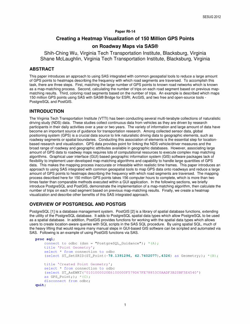
In the above example, Part A lets SAS access the PostgreSQL database via an ODBC connection [3]. In Part B, the PostGIS function, ST_Point, creates point geometry for a GPS point and the ST_SetSRID function specifies the spatial reference system used by the GPS receiver which was used for collecting this data. The result is shown in the upper portion of Figure 1. In Part C above, the function, ST_AsEWKT, returns the created geometry representation in Well-Known-Text (WKT) format with a spatial reference system identifier (SRID) metadata. The result is shown in the bottom part of Figure 1 which matches the latitude and longitude coordinates input in Part B of the SAS code.

Figure 1. SAS PROC SQL Output

PREPARATION OF DATA SETS

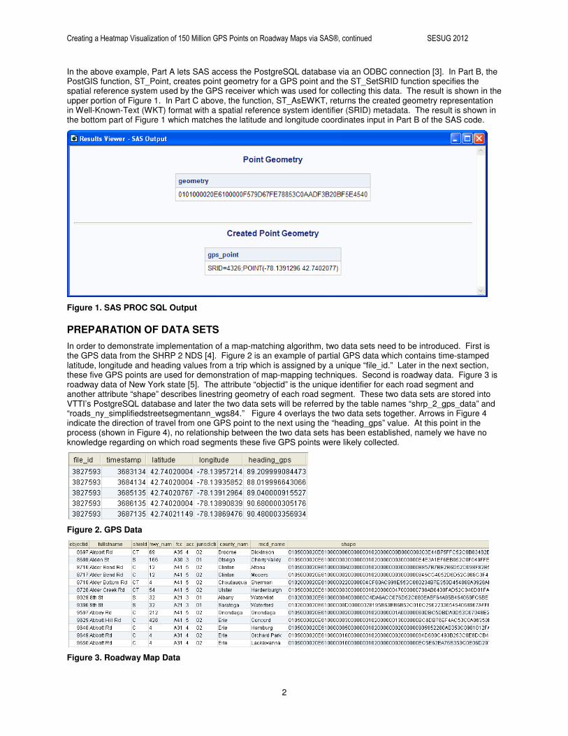
In order to demonstrate implementation of a map-matching algorithm, two data sets need to be introduced. First is the GPS data from the SHRP 2 NDS [4]. Figure 2 is an example of partial GPS data which contains time-stamped latitude, longitude and heading values from a trip which is assigned by a unique “file_id.” Later in the next section, these five GPS points are used for demonstration of map-mapping techniques. Second is roadway data. Figure 3 is roadway data of New York state [5]. The attribute “objectid” is the unique identifier for each road segment and another attribute “shape” describes linestring geometry of each road segment. These two data sets are stored into VTTI’s PostgreSQL database and later the two data sets will be referred by the table names “shrp_2_gps_data” and “roads_ny_simplifiedstreetsegmentann_wgs84.” Figure 4 overlays the two data sets together. Arrows in Figure 4 indicate the direction of travel from one GPS point to the next using the “heading_gps” value. At this point in the process (shown in Figure 4), no relationship between the two data sets has been established, namely we have no knowledge regarding on which road segments these five GPS points were likely collected.

Figure 2. GPS Data

Figure 3. Roadway Map Data


3

Figure 4. GPS Data on Roadway Map

MAP MATCHING

Map matching is a process of associating GPS traces on road segments. A simple and intuitive way is mapping GPS data to a nearby road. The following SAS sample code illustrates how to search for the closest road segment for one GPS point (the first point shown in Figure 2).

proc sql;

connect to odbc (dsn = "PostgreSQL_Guidance");

title 'Map Matching Result (Nearest Neighbor)';

create table mm_result as


(select gps.file_id, gps.timestamp, gps.latitude, gps.longitude,

gps.heading_gps,

road.objectid, road.fullstname, road.shield, road.hwy_num, road.fcc, road.acc,

road.jurisdicti, road.county_nam, road.mcd_name

from scwu.shrp_2_gps_data as gps,

scwu.roads_ny_simplifiedstreetsegmentann_wgs84 as road

where file_id = 3827593 and timestamp = 3683134 /* (D) */

order by ST_DISTANCE(road.shape, ST_SetSRID(ST_Point(gps.longitude,

gps.latitude),4326)) /* (E) */

limit 1;);


quit;

In Part D, the WHERE statement selects one GPS point from the sample data (Figure 2). Part E, the PostGIS ST_DISTANCE function calculates distance between two geometries which are the collected GPS point and New York roadway map. Since results are ordered by distance, the first record is always the nearest road segment to GPS data. Results of applying the same map-matching algorithm to all five GPS points are shown in the following figure.

Figure 5. Map-Matching Results

For clarity, the above code conducts the mapping for one GPS point. In practice, this code uses SAS Macro to iterate through as many GPS points as are in the data set.

From Figure 4, these five GPS points actually travel on W Buffalo Street and, from Figure 2, GPS heading values (~90 deg) also indicate the vehicle moves toward the East. However, the map-matching result has one GPS point mapped on S Maple Street. Using shortest distance or nearest neighbor as mapping criteria might be inaccurate


4

when there are multiple roads near a GPS point such as at intersections. This mistaken classification can be fixed if GPS heading values are considered. In this case, PostGIS and SAS come in handy to implement algorithm improvements with user-developed techniques. The following SAS sample code is an extension from the previous SAS sample code. It changes focus on the third GPS point, measures bearing of road segments, and calculates the difference between GPS heading of the vehicle and bearing of road segments.

proc sql;


title 'Map Matching Result (Nearest Neighbor & Match Heading)';




gps.heading_gps,


road.jurisdicti, road.county_nam, road.mcd_name,

ST_Azimuth(endpoint(road.shape), startpoint(road.shape))/(2*pi())*360

as road_bearing, /* (F) */

abs(ST_Azimuth(endpoint(road.shape), startpoint(road.shape))/(2*pi())*360 -

gps.heading_gps) as heading_diff /* (G) */



where file_id = 3827593 and timestamp = 3685135


gps.latitude),4326))

limit 3;);


quit;

Part F uses the PostGIS function, ST_Azimuth, to measure bearing of road segments based on two nodes of each road segment. Part G calculates difference between GPS heading and calculated bearing values from Part F. The SAS output in Figure 6 shows the top three closest road segments and only the W Buffalo Street bearing matches direction of what GPS heading indicates.


proc sql;


title 'Map Matching Result (Nearest Neighbor & Match Heading)';




gps.heading_gps,


road.jurisdicti, road.county_nam, road.mcd_name,

ST_Azimuth(endpoint(road.shape), startpoint(road.shape))/(2*pi())*360

as road_bearing,


gps.heading_gps) as heading_diff



where file_id = 3827593 and timestamp = 3685135 and


gps.heading_gps) <= 25 /* (H) */


5


gps.latitude),4326))

limit 1;);


quit;

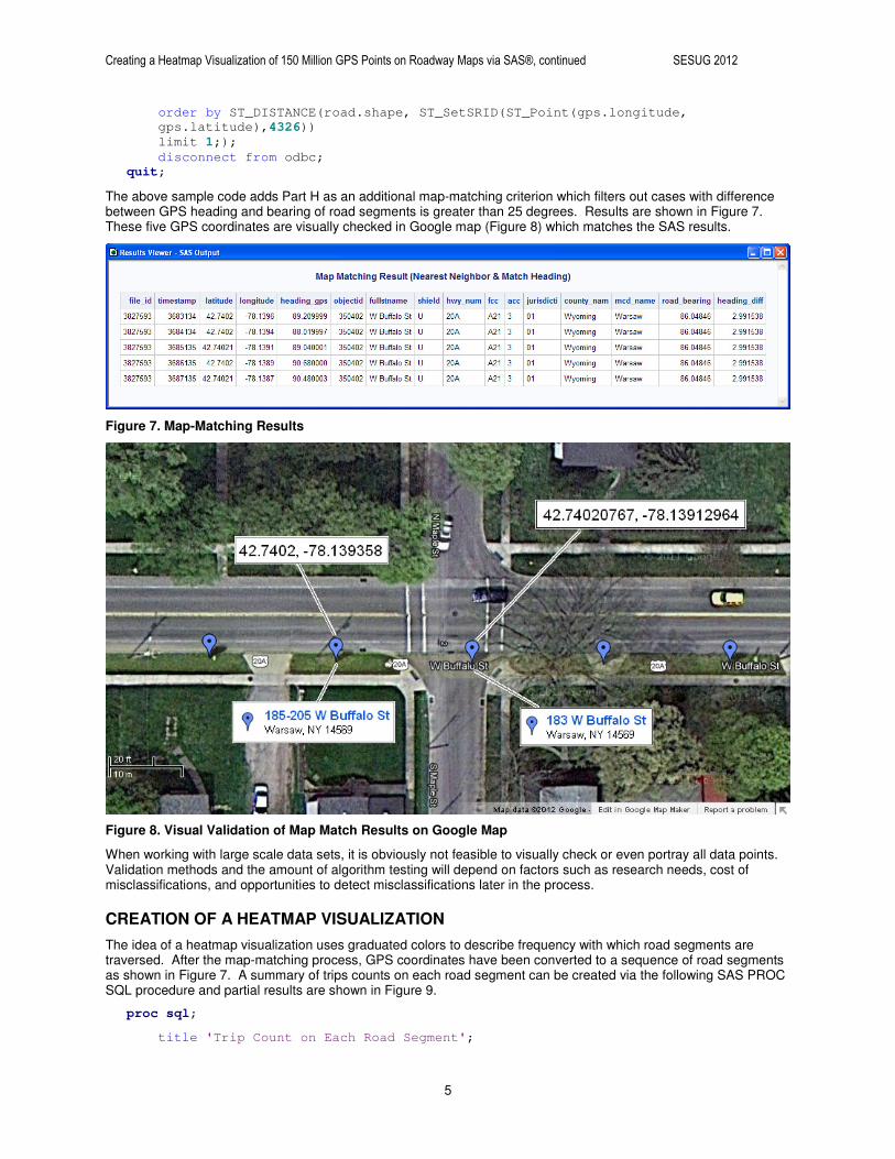
The above sample code adds Part H as an additional map-matching criterion which filters out cases with difference between GPS heading and bearing of road segments is greater than 25 degrees. Results are shown in Figure 7. These five GPS coordinates are visually checked in Google map (Figure 8) which matches the SAS results.


Figure 8. Visual Validation of Map Match Results on Google Map

When working with large scale data sets, it is obviously not feasible to visually check or even portray all data points. Validation methods and the amount of algorithm testing will depend on factors such as research needs, cost of misclassifications, and opportunities to detect misclassifications later in the process.

CREATION OF A HEATMAP VISUALIZATION

The idea of a heatmap visualization uses graduated colors to describe frequency with which road segments are traversed. After the map-matching process, GPS coordinates have been converted to a sequence of road segments as shown in Figure 7. A summary of trips counts on each road segment can be created via the following SAS PROC SQL procedure and partial results are shown in Figure 9.

proc sql;

title 'Trip Count on Each Road Segment';


6

create table trip_counts as

select objectid, count(distinct file_id) as trip_counts

from mm_result

group by objectid;

quit;

Figure 9. SAS PROC SQL Output

SAS Bridge for ESRI [6] enables ArcGIS [7] to read a SAS data set which allows ArcGIS to create heatmaps based on the summary in Figure 9. Through the ArcGIS GUI, first, add the SAS data set and the New York roadway map into ArcMap. Then join the two imported data sets via the attribute “objectid” as shown in Figure 10. After ArcGIS spatial joins trip counts to the map data using “objectid,” information of trip counts is added to the layer of roadway map. The user can then modify layer properties and use quantity “trip_counts” to specify the color in which road segments with different numbers of trips will be portrayed (Figure 11). Finally, a heatmap visualization has been created.

Figure 10. Creation of Heatmap Visualization in ArcGIS


7

Figure 11. Creation of Heatmap Visualization in ArcGIS

The following figures are sample heatmap visualizations from some of the SHRP 2 NDS data. Figure 12 shows trips traveled only on interstates in the Seattle Washington area. Figure 13 shows trips that have been associated with interstates and U.S. highways in North Carolina. Figure 14 zooms in to show mapping of these data points to road segments in the Raleigh area.

Figure 12. Heatmap Visualization


8




9

ADDITIONAL BENEFITS

There are a number of direct and ancillary benefits of the described approach. As mentioned in the introduction, the process described here is much faster than GUI based methods. More specifically though, GUI methods would require a user to manually break up the task into subtasks and monitor completion of each portion. The process described here lends itself to being divided up in an automated way across multiple computers, thereby reducing the overall time to completion [8]. For example, the 156 hour example could be divided by four if four computers are used. The method also permits process monitoring and graceful recovery in the event of a process interruption. For example, the user can continuously monitor the accumulation of results in the database and identify when an interruption occurred.

CONCLUSION

Attributes included in GISs are important for transportation research, but the capability of efficiently processing large data in GUI-based GIS software is limited. Integrating SAS with PostgreSQL, PostGIS, and ArcGIS provides usable solutions to accomplish location-based associations of large quantities of data. This paper demonstrates an efficient approach to associate GPS data to roadway maps and create informative heatmap visualizations.

REFERENCES

1. PostgreSQL. http://www.postgresql.org/.

2. PostGIS. http://postgis.refractions.net/.

3. SAS Institute, 2011, SAS/ACCESS® 9.3 for Relational Databases Reference. Cary, NC: SAS Institute, Inc. http://support.sas.com/documentation/cdl/en/acreldb/63144/PDF/default/acreldb.pdf.

4. Strategic Highway Research Program 2. http://www.shrp2nds.us/.

5. New York State Geographic Information Systems (GIS) Clearinghouse. http://gis.ny.gov/gisdata/inventories/details.cfm?dsid=932&nysgis=#.

6. Massengill, Darrell. 2007. “Making Business Decisions Using SAS Mapping Technologies”. Proceedings of the SAS Global Forum 2007 Conference. Cary, NC. SAS Institute Inc. http://support.sas.com/rnd/papers/sgf07/sgf2007-map.pdf.

7. ESRI ArcGIS. http://www.esri.com/.

8. Wu, Shih-Ching and McLaughlin, Shane. 2012. “Tips for Using SAS to Manipulate Large-scale Data in Databases“. the NorthEast SAS Users Group (NESUG) 2012 Conference.

ACKNOWLEDGMENTS

The authors would like to acknowledge the research participants and the external contributions which made this work possible. The data used in this study were collected as part of the SHRP 2 Naturalistic Driving Study, which is sponsored by the Transportation Research Board of the National Academies. The methods developed and described in this paper were developed with funds from the National Surface Transportation Safety Center for Excellence.

CONTACT INFORMATION

Your comments and questions are valued and encouraged. Contact the authors at:

Shih-Ching Wu Shane McLaughlin Virginia Tech Transportation Institute Virginia Tech Transportation Institute 3500 Transportation Research Plaza 3500 Transportation Research Plaza Blacksburg, VA, 24061 Blacksburg, VA, 24061 540-231-1091 540-231-1077 [email protected] [email protected] http://www.vtti.vt.edu http://www.vtti.vt.edu

SAS and all other SAS Institute Inc. product or service names are registered trademarks or trademarks of SAS Institute Inc. in the USA and other countries. ® indicates USA registration.

Other brand and product names are trademarks of their respective companies.

Documents

Paper RI-14 Creating a Heatmap Visualization of 150 ...analytics.ncsu.edu/sesug/2012/RI-14.pdf · Creating a Heatmap Visualization of 150 Million GPS ... Wu, Virginia Tech Transportation