Paper - The Robotics Institute - Carnegie Mellon University

Robotics and Autonomous Systems ( ) –

Contents lists available at SciVerse ScienceDirect

Robotics and Autonomous Systems

journal homepage: www.elsevier.com/locate/robot

Autonomous landing at unprepared sites by a full-scale helicopterSebastian Scherer ∗, Lyle Chamberlain, Sanjiv SinghRobotics Institute, Carnegie Mellon University, Pittsburgh, PA, USA

a r t i c l e i n f o

Article history:Received 23 June 2011Received in revised form24 March 2012Accepted 8 September 2012Available online xxxx

Keywords:UAVRotorcraft3D perceptionLidarLanding zone selection

a b s t r a c t

Helicopters are valuable since they can land at unprepared sites; however, current unmanned helicoptersare unable to select or validate landing zones (LZs) and approach paths. For operation in unknown terrainit is necessary to assess the safety of a LZ. In this paper, we describe a lidar-based perception system thatenables a full-scale autonomous helicopter to identify and land in previously unmapped terrain with nohuman input.

We describe the problem, real-time algorithms, perception hardware, and results. Our approachhas extended the state of the art in terrain assessment by incorporating not only plane fitting, but byalso considering factors such as terrain/skid interaction, rotor and tail clearance, wind direction, clearapproach/abort paths, and ground paths.

In results from urban and natural environments we were able to successfully classify LZs from pointcloud maps. We also present results from 8 successful landing experiments with varying ground clutterand approach directions. The helicopter selected its own landing site, approaches, and then proceedsto land. To our knowledge, these experiments were the first demonstration of a full-scale autonomoushelicopter that selected its own landing zones and landed.

© 2012 Elsevier B.V. All rights reserved.

1. Introduction

Safe autonomous flight at lowaltitude is essential forwidespreadacceptance of aircraft that must complete missions close to theground, and such capability is widely sought. For example, searchand rescue operations in the setting of a natural disaster allow dif-ferent vantage points at low altitude. Likewise, UAVs performingreconnaissance for the police, news stations or the military mustfly at low altitude in the presence of obstacles. Large rotorcraft canfly at high altitude, but however have to come close to the groundduring landing and takeoff. So far unmanned full-scale rotorcrafthave to land on prepared land at prepared sites with prior knowl-edge of obstacle-free trajectories.

Assessing a landing zone (LZ) reliably is essential for safeoperation of vertical takeoff and landing (VTOL) aerial vehiclesthat land at unimproved locations. Currently an UAV operatorhas to rely on visual assessment to make an approach decision;however, visual information from afar is insufficient to judgeslope and detect small obstacles. Prior work in landing siteevaluation has modeled LZ quality based on plane fitting, whichonly partly represents the interaction between vehicle and ground.Additionally, we want to be able to guide an unmanned rotorcraftto a safe landing location.

∗ Corresponding author.E-mail addresses: [email protected] (S. Scherer), [email protected]

(L. Chamberlain), [email protected] (S. Singh).

A NASA study of rotorcraft accidents from 1963 to 1997 foundthat collisions with objects, hard landings, and roll-overs wereresponsible for over 36% of the incidents [1]. A partial cause foraccidents is a lack of situational awareness of the pilot regardingthe suitability of landing sites. Reliable evaluation of landing siteswill increase the safety of operation of rotorcraft by presentingvital information to the pilot or unmanned aerial vehicle before alanding approach.

Our algorithmic approach consists of a coarse evaluation basedon slope and roughness criteria, a fine evaluation for skid contact,and body clearance of a location. Additionally we consider theground path to a goal location and approach paths to the landingsite. We investigated whether the evaluation is correct for usingterrain maps collected from a helicopter and tested landingin unknown environments. This article defines the problem ofevaluation, describes our incremental real-time algorithm andinformation gain map, and discusses the effectiveness of ourapproach.

We show results from two aircraft-based perception systems.The first is a downward-scanning lidar mounted on a manned EC-135 helicopter. The second system is a 3-D lidar-based perceptionsystem that guides the Unmanned Little Bird helicopter in fully-autonomous flight and landings. In results from urban and naturalenvironments from these two different helicopter platforms, wewere able to successfully classify and land at LZs from point cloudmaps collected on a helicopter in real-time. The presentedmethodenables detailed assessment of LZs from pattern altitude beforedescent.

0921-8890/$ – see front matter© 2012 Elsevier B.V. All rights reserved.doi:10.1016/j.robot.2012.09.004

http://dx.doi.org/10.1016/j.robot.2012.09.004

http://www.elsevier.com/locate/robot

http://www.elsevier.com/locate/robot

mailto:[email protected]



http://dx.doi.org/10.1016/j.robot.2012.09.004

2 S. Scherer et al. / Robotics and Autonomous Systems ( ) –

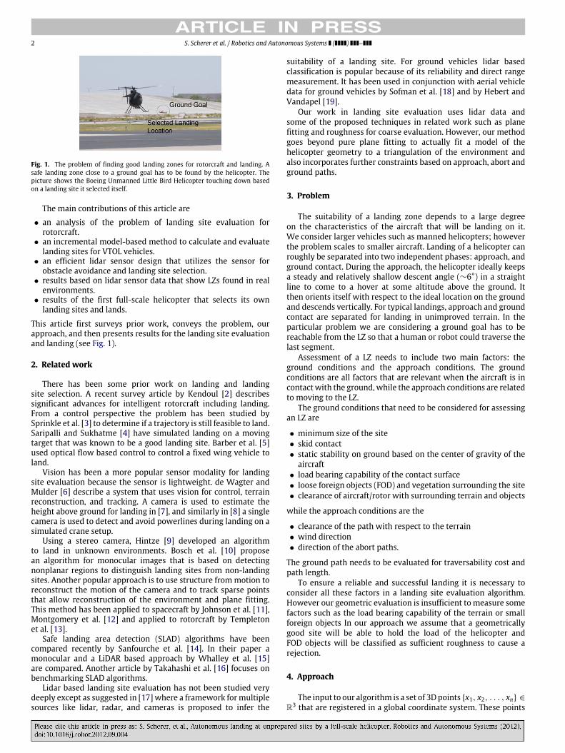
Fig. 1. The problem of finding good landing zones for rotorcraft and landing. Asafe landing zone close to a ground goal has to be found by the helicopter. Thepicture shows the Boeing Unmanned Little Bird Helicopter touching down basedon a landing site it selected itself.

The main contributions of this article are

• an analysis of the problem of landing site evaluation forrotorcraft.

• an incremental model-based method to calculate and evaluatelanding sites for VTOL vehicles.

• an efficient lidar sensor design that utilizes the sensor forobstacle avoidance and landing site selection.

• results based on lidar sensor data that show LZs found in realenvironments.

• results of the first full-scale helicopter that selects its ownlanding sites and lands.

This article first surveys prior work, conveys the problem, ourapproach, and then presents results for the landing site evaluationand landing (see Fig. 1).

2. Related work

There has been some prior work on landing and landingsite selection. A recent survey article by Kendoul [2] describessignificant advances for intelligent rotorcraft including landing.From a control perspective the problem has been studied bySprinkle et al. [3] to determine if a trajectory is still feasible to land.Saripalli and Sukhatme [4] have simulated landing on a movingtarget that was known to be a good landing site. Barber et al. [5]used optical flow based control to control a fixed wing vehicle toland.

Vision has been a more popular sensor modality for landingsite evaluation because the sensor is lightweight. de Wagter andMulder [6] describe a system that uses vision for control, terrainreconstruction, and tracking. A camera is used to estimate theheight above ground for landing in [7], and similarly in [8] a singlecamera is used to detect and avoid powerlines during landing on asimulated crane setup.

Using a stereo camera, Hintze [9] developed an algorithmto land in unknown environments. Bosch et al. [10] proposean algorithm for monocular images that is based on detectingnonplanar regions to distinguish landing sites from non-landingsites. Another popular approach is to use structure frommotion toreconstruct the motion of the camera and to track sparse pointsthat allow reconstruction of the environment and plane fitting.This method has been applied to spacecraft by Johnson et al. [11],Montgomery et al. [12] and applied to rotorcraft by Templetonet al. [13].

Safe landing area detection (SLAD) algorithms have beencompared recently by Sanfourche et al. [14]. In their paper amonocular and a LiDAR based approach by Whalley et al. [15]are compared. Another article by Takahashi et al. [16] focuses onbenchmarking SLAD algorithms.

Lidar based landing site evaluation has not been studied verydeeply except as suggested in [17] where a framework formultiplesources like lidar, radar, and cameras is proposed to infer the

suitability of a landing site. For ground vehicles lidar basedclassification is popular because of its reliability and direct rangemeasurement. It has been used in conjunction with aerial vehicledata for ground vehicles by Sofman et al. [18] and by Hebert andVandapel [19].

Our work in landing site evaluation uses lidar data andsome of the proposed techniques in related work such as planefitting and roughness for coarse evaluation. However, our methodgoes beyond pure plane fitting to actually fit a model of thehelicopter geometry to a triangulation of the environment andalso incorporates further constraints based on approach, abort andground paths.

3. Problem

The suitability of a landing zone depends to a large degreeon the characteristics of the aircraft that will be landing on it.We consider larger vehicles such as manned helicopters; howeverthe problem scales to smaller aircraft. Landing of a helicopter canroughly be separated into two independent phases: approach, andground contact. During the approach, the helicopter ideally keepsa steady and relatively shallow descent angle (∼6°) in a straightline to come to a hover at some altitude above the ground. Itthen orients itself with respect to the ideal location on the groundand descends vertically. For typical landings, approach and groundcontact are separated for landing in unimproved terrain. In theparticular problem we are considering a ground goal has to bereachable from the LZ so that a human or robot could traverse thelast segment.

Assessment of a LZ needs to include two main factors: theground conditions and the approach conditions. The groundconditions are all factors that are relevant when the aircraft is incontact with the ground, while the approach conditions are relatedto moving to the LZ.

The ground conditions that need to be considered for assessingan LZ are

• minimum size of the site• skid contact• static stability on ground based on the center of gravity of the

aircraft• load bearing capability of the contact surface• loose foreign objects (FOD) and vegetation surrounding the site• clearance of aircraft/rotor with surrounding terrain and objects

while the approach conditions are the

• clearance of the path with respect to the terrain• wind direction• direction of the abort paths.

The ground path needs to be evaluated for traversability cost andpath length.

To ensure a reliable and successful landing it is necessary toconsider all these factors in a landing site evaluation algorithm.However our geometric evaluation is insufficient to measure somefactors such as the load bearing capability of the terrain or smallforeign objects In our approach we assume that a geometricallygood site will be able to hold the load of the helicopter andFOD objects will be classified as sufficient roughness to cause arejection.

4. Approach

The input to our algorithm is a set of 3Dpoints {x1, x2, . . . , xn} ∈

R3 that are registered in a global coordinate system. These points

S. Scherer et al. / Robotics and Autonomous Systems ( ) – 3

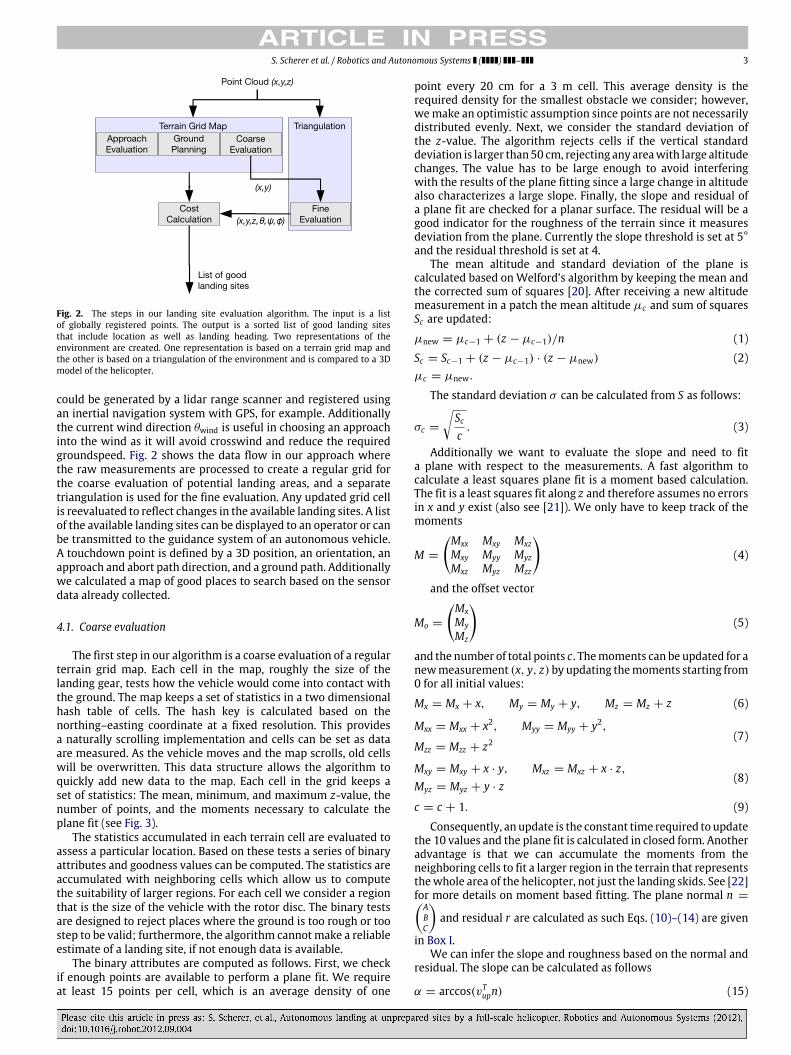
Fig. 2. The steps in our landing site evaluation algorithm. The input is a listof globally registered points. The output is a sorted list of good landing sitesthat include location as well as landing heading. Two representations of theenvironment are created. One representation is based on a terrain grid map andthe other is based on a triangulation of the environment and is compared to a 3Dmodel of the helicopter.

could be generated by a lidar range scanner and registered usingan inertial navigation system with GPS, for example. Additionallythe current wind direction θwind is useful in choosing an approachinto the wind as it will avoid crosswind and reduce the requiredgroundspeed. Fig. 2 shows the data flow in our approach wherethe raw measurements are processed to create a regular grid forthe coarse evaluation of potential landing areas, and a separatetriangulation is used for the fine evaluation. Any updated grid cellis reevaluated to reflect changes in the available landing sites. A listof the available landing sites can be displayed to an operator or canbe transmitted to the guidance system of an autonomous vehicle.A touchdown point is defined by a 3D position, an orientation, anapproach and abort path direction, and a ground path. Additionallywe calculated a map of good places to search based on the sensordata already collected.

4.1. Coarse evaluation

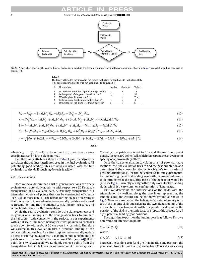
The first step in our algorithm is a coarse evaluation of a regularterrain grid map. Each cell in the map, roughly the size of thelanding gear, tests how the vehicle would come into contact withthe ground. The map keeps a set of statistics in a two dimensionalhash table of cells. The hash key is calculated based on thenorthing–easting coordinate at a fixed resolution. This providesa naturally scrolling implementation and cells can be set as dataare measured. As the vehicle moves and the map scrolls, old cellswill be overwritten. This data structure allows the algorithm toquickly add new data to the map. Each cell in the grid keeps aset of statistics: The mean, minimum, and maximum z-value, thenumber of points, and the moments necessary to calculate theplane fit (see Fig. 3).

The statistics accumulated in each terrain cell are evaluated toassess a particular location. Based on these tests a series of binaryattributes and goodness values can be computed. The statistics areaccumulated with neighboring cells which allow us to computethe suitability of larger regions. For each cell we consider a regionthat is the size of the vehicle with the rotor disc. The binary testsare designed to reject places where the ground is too rough or toostep to be valid; furthermore, the algorithm cannotmake a reliableestimate of a landing site, if not enough data is available.

The binary attributes are computed as follows. First, we checkif enough points are available to perform a plane fit. We requireat least 15 points per cell, which is an average density of one

point every 20 cm for a 3 m cell. This average density is therequired density for the smallest obstacle we consider; however,wemake an optimistic assumption since points are not necessarilydistributed evenly. Next, we consider the standard deviation ofthe z-value. The algorithm rejects cells if the vertical standarddeviation is larger than50 cm, rejecting any areawith large altitudechanges. The value has to be large enough to avoid interferingwith the results of the plane fitting since a large change in altitudealso characterizes a large slope. Finally, the slope and residual ofa plane fit are checked for a planar surface. The residual will be agood indicator for the roughness of the terrain since it measuresdeviation from the plane. Currently the slope threshold is set at 5°and the residual threshold is set at 4.

The mean altitude and standard deviation of the plane iscalculated based on Welford’s algorithm by keeping the mean andthe corrected sum of squares [20]. After receiving a new altitudemeasurement in a patch the mean altitude µc and sum of squaresSc are updated:

µnew = µc−1 + (z − µc−1)/n (1)

Sc = Sc−1 + (z − µc−1) · (z − µnew) (2)µc = µnew.

The standard deviation σ can be calculated from S as follows:

σc =

Scc

. (3)

Additionally we want to evaluate the slope and need to fita plane with respect to the measurements. A fast algorithm tocalculate a least squares plane fit is a moment based calculation.The fit is a least squares fit along z and therefore assumes no errorsin x and y exist (also see [21]). We only have to keep track of themoments

M =

Mxx Mxy MxzMxy Myy MyzMxz Myz Mzz

(4)

and the offset vector

Mo =

MxMyMz

(5)

and the number of total points c. Themoments can be updated for anewmeasurement (x, y, z) by updating themoments starting from0 for all initial values:

Mx = Mx + x, My = My + y, Mz = Mz + z (6)

Mxx = Mxx + x2, Myy = Myy + y2,

Mzz = Mzz + z2(7)

Mxy = Mxy + x · y, Mxz = Mxz + x · z,Myz = Myz + y · z

(8)

c = c + 1. (9)

Consequently, an update is the constant time required to updatethe 10 values and the plane fit is calculated in closed form. Anotheradvantage is that we can accumulate the moments from theneighboring cells to fit a larger region in the terrain that representsthewhole area of the helicopter, not just the landing skids. See [22]for more details on moment based fitting. The plane normal n =

ABC

and residual r are calculated as such Eqs. (10)–(14) are given

in Box I.We can infer the slope and roughness based on the normal and

residual. The slope can be calculated as follows

α = arccos(vTupn) (15)


Fig. 3. A flow chart showing the control flow of evaluating a patch in the terrain grid map. Only if all binary attributes shown in Table 1 are valid a landing zone will beconsidered.

Table 1The binary attributes considered in the coarse evaluation for landing site evaluation. Onlyif all operations evaluate to true can a landing site be available.

# Description Symbol Operator Value

1 Do we have more than x points for a plane fit? c > 152 Is the spread of the points less than x cm? σn < 503 Was the plane fit successful? = True4 Is the residual for the plane fit less than x? r < 45 Is the slope of the plane less than x degrees? α < 5

Mn = M2xyc − 2 · MxMxyMy, +M2

xMyy + (M2y − cMyy)Mxx (10)

A = (M2yMxz − (MxMyz + MxyMz)My + c(−MxzMyy + MxyMyz) + XxMYYMz)/Mn (11)

B = (−(MxyMz + MxzMy)Mx + cMxyMxz + M2xMyz + Mxx(−cMyz + MyMz))/Mn (12)

C = (−(MxMyz + MxzMy)Mxy + MxMxzMyy + M2xyMz + Mxx(MYMyz − MyyMz))/Mn (13)

r =

C2c + 2ACMx + A2Mxx + 2BCMx + 2ABMxy + B2MYY − 2CMz − 2AMxz − 2BMyz + Mzz /c. (14)

Box I.

where vup = (0, 0, −1) is the up vector (in north-east-downcoordinates) and n is the plane normal.

If all the binary attributes shown in Table 1 pass, the algorithmcalculates the goodness attributes used in the final evaluation. Allpotentially good landing sites are now evaluated with the fineevaluation to decide if touching down is feasible.

4.2. Fine evaluation

Once we have determined a list of general locations, we finelyevaluate each potentially good site with respect to a 2D Delaunaytriangulation of all available data. A Delaunay triangulation is atriangular network of points that can be constructed efficiently(see [23] for more details). The reason for this staged processing isthat it is easier to knowwhen to incrementally update a cell-basedrepresentation, and the incremental calculation for the coarse gridis much faster than for the triangulation.

While the coarse evaluation considers the plane geometry androughness of a landing site, the triangulation tries to simulatethe helicopter static contact with the surface. In our experimentswith a full scale unmanned helicopter it was possible to control atouch down to within about 30 cm even in crosswind. Thereforewe assume in this evaluation that a precision landing of thevehicle will be possible. As a first step we incrementally updatea hierarchical triangulation with amaximum number of points perpatch area. For the implementation we use CGAL (see [24]). If thepoint density is exceeded, we randomly remove points from thetriangulation to keep below a maximum amount of memory used.

Currently, the patch size is set to 3 m and the maximum pointdensity is set to 200points/cell,which corresponds to an evenpointspacing of approximately 20 cm.

Once the coarse evaluation calculates a list of potential (x, y)locations, the fine evaluation tries to find the best orientation anddetermines if the chosen location is feasible. We test a series ofpossible orientations θ of the helicopter (8 in our experiments)by intersecting the virtual landing gear with the measured terrainto determine what the resulting pose of the helicopter would be(also see Fig. 4). Currently our algorithmonlyworks for two landingskids, which is a very common configuration of landing gear.

First we determine the intersections of the skids with thetriangulation by walking along the two lines representing thelanding skids, and extract the height above ground as shown inFig. 5. Now we assume that the helicopter’s center of gravity is ontop of the landing skids and calculate the two highest points of theintersection. These twopointswill be the points that determine theposition of the skid in the static case. We repeat this process for alleight potential landing gear positions.

The algorithm to position the landing gear is as follows. First wedetermine all intersection points

pli = (xli, yli, z

li) (16)

where

pli ∈ R3, i ∈ {1, . . . , n} (17)

between the landing gear l and the triangulation and partition thepoints into two sets: Points aft, ali, and in front,f li , of a distance along


Fig. 4. The flow chart of the fine evaluation algorithm. The pose of the helicopter is calculated based on a (x, y, θ) position and heading. If the pose is calculated successfullya surface model of the aerial vehicle is evaluated.

Fig. 5. Illustration of skid-triangulation contact. The skids in contact with the triangulation determine the roll and pitch of the vehicle. A good contact is characterized by asmall angle and small area between the skid and triangulation.

the landing gear. Currentlywe set the distance to be half the lengthof the landing gear because we assume that the center of mass iscentered on top of the landing gear; however. this position can bechanged depending on the mass distribution.

Next we look at the z-values and find the maximum z-value inthe first and in the second half of the landing skid for each side:

plaft = argmax(ali) (18)

plfront = argmax(f li ). (19)

Aminimum distance between paft and pfront is set to ensure thatthe slope will fit to a stable value. Now that we know how thelanding gear will be positioned, we calculate the area between theline of the skid and the triangulation to get a measure of contactarea. For example, if we were to land centered on railroad tracksat an 90° angle our skids would rest on the rails because theyare the highest points above the ground. In this case even thoughthe roll, pitch, and roughness will be small (rails are very smalldeviations from the ground and usually level) the integral of the

area under the landing skids will have a large value because mostof the landing skid is elevated above the ground. For skids in fullcontact with the ground the integral would be zero.

The next step is to determine the roll and pitch of the helicopterwhen it is in contact with the ground. We use the center of thetwo landing skid lines to determine the roll angle. Finally we usethe lower landing gear line to calculate pitch because the centerof gravity will shift towards that line. Using this algorithm we arenow able to predict the position and orientation of the helicopterwhen it is in contact with the ground. The roll angle α is calculatedfrom the interpolated centers plc of the skids

plc =pln − pl1

2(20)

α = arctan 2z2c − z1c ,

(x2c − x1c )2 + (y2c − y1c )2

. (21)

The pitch of the helicopter depends on the roll angle sincemore weight will shift towards the lower skid. The pitch angle β


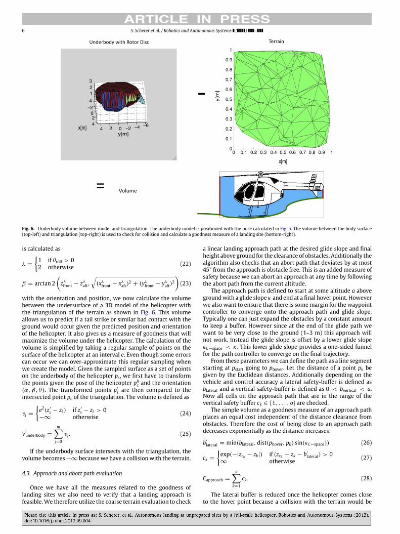
Fig. 6. Underbody volume between model and triangulation. The underbody model is positioned with the pose calculated in Fig. 5. The volume between the body surface(top-left) and triangulation (top-right) is used to check for collision and calculate a goodness measure of a landing site (bottom-right).

is calculated as

λ =

1 if θroll > 02 otherwise (22)

β = arctan 2zλfront − zλ

aft,

(xλ

front − xλaft)

2 + (yλfront − yλ

aft)2

(23)

with the orientation and position, we now calculate the volumebetween the undersurface of a 3D model of the helicopter withthe triangulation of the terrain as shown in Fig. 6. This volumeallows us to predict if a tail strike or similar bad contact with theground would occur given the predicted position and orientationof the helicopter. It also gives us a measure of goodness that willmaximize the volume under the helicopter. The calculation of thevolume is simplified by taking a regular sample of points on thesurface of the helicopter at an interval e. Even though some errorscan occur we can over-approximate this regular sampling whenwe create the model. Given the sampled surface as a set of pointson the underbody of the helicopter ps, we first have to transformthe points given the pose of the helicopter phc and the orientation(α, β, θ). The transformed points p′

s are then compared to theintersected point pt of the triangulation. The volume is defined as

vj =

e2(z ′

s − zt) if z ′

s − zt > 0−∞ otherwise (24)

Vunderbody =

mj=0

vj. (25)

If the underbody surface intersects with the triangulation, thevolume becomes−∞ becausewe have a collisionwith the terrain.

4.3. Approach and abort path evaluation

Once we have all the measures related to the goodness oflanding sites we also need to verify that a landing approach isfeasible.We therefore utilize the coarse terrain evaluation to check

a linear landing approach path at the desired glide slope and finalheight above ground for the clearance of obstacles. Additionally thealgorithm also checks that an abort path that deviates by at most45° from the approach is obstacle free. This is an addedmeasure ofsafety because we can abort an approach at any time by followingthe abort path from the current altitude.

The approach path is defined to start at some altitude a abovegroundwith a glide slope κ and end at a final hover point. Howeverwe also want to ensure that there is somemargin for the waypointcontroller to converge onto the approach path and glide slope.Typically one can just expand the obstacles by a constant amountto keep a buffer. However since at the end of the glide path wewant to be very close to the ground (1–3 m) this approach willnot work. Instead the glide slope is offset by a lower glide slopeκC−space < κ . This lower glide slope provides a one-sided funnelfor the path controller to converge on the final trajectory.

From these parameterswe can define the path as a line segmentstarting at pstart going to phover. Let the distance of a point pk begiven by the Euclidean distances. Additionally depending on thevehicle and control accuracy a lateral safety-buffer is defined asblateral and a vertical safety-buffer is defined as 0 < bvertical < a.Now all cells on the approach path that are in the range of thevertical safety buffer ck ∈ {1, . . . , o} are checked.

The simple volume as a goodness measure of an approach pathplaces an equal cost independent of the distance clearance fromobstacles. Therefore the cost of being close to an approach pathdecreases exponentially as the distance increases:

b′

lateral = min(blateral, dist(phover, pk) sin(κC−space)) (26)

ck =

exp(−|zck − zk|) if (zck − zk − b′

lateral) > 0∞ otherwise (27)

Capproach =

ok=1

ck. (28)

The lateral buffer is reduced once the helicopter comes closeto the hover point because a collision with the terrain would be


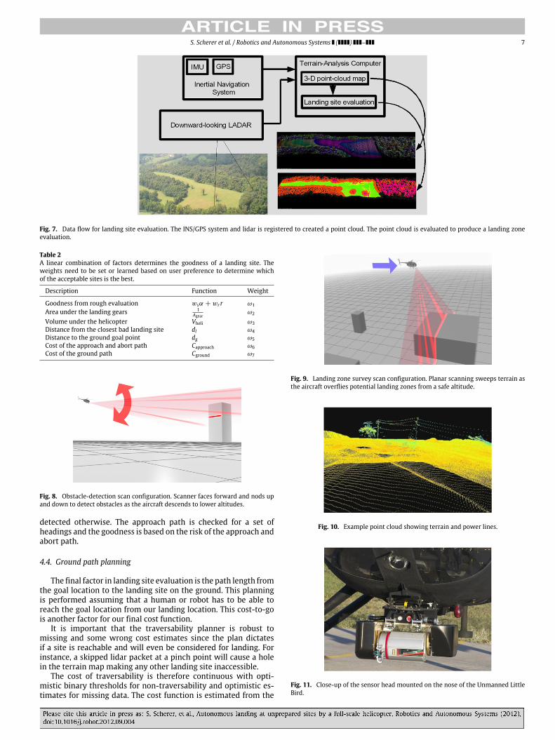
Fig. 7. Data flow for landing site evaluation. The INS/GPS system and lidar is registered to created a point cloud. The point cloud is evaluated to produce a landing zoneevaluation.

Table 2A linear combination of factors determines the goodness of a landing site. Theweights need to be set or learned based on user preference to determine whichof the acceptable sites is the best.

Description Function Weight

Goodness from rough evaluation wsα + wr r ω1

Area under the landing gears 1Agear

ω2

Volume under the helicopter Vheli ω3Distance from the closest bad landing site dl ω4Distance to the ground goal point dg ω5Cost of the approach and abort path Capproach ω6Cost of the ground path Cground ω7

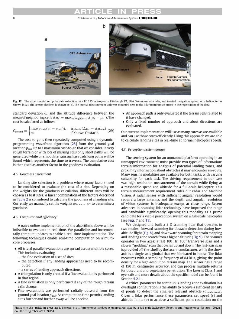
Fig. 8. Obstacle-detection scan configuration. Scanner faces forward and nods upand down to detect obstacles as the aircraft descends to lower altitudes.

detected otherwise. The approach path is checked for a set ofheadings and the goodness is based on the risk of the approach andabort path.

4.4. Ground path planning

The final factor in landing site evaluation is the path length fromthe goal location to the landing site on the ground. This planningis performed assuming that a human or robot has to be able toreach the goal location from our landing location. This cost-to-gois another factor for our final cost function.

It is important that the traversability planner is robust tomissing and some wrong cost estimates since the plan dictatesif a site is reachable and will even be considered for landing. Forinstance, a skipped lidar packet at a pinch point will cause a holein the terrain map making any other landing site inaccessible.

The cost of traversability is therefore continuous with opti-mistic binary thresholds for non-traversability and optimistic es-timates for missing data. The cost function is estimated from the

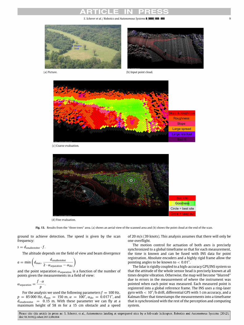
Fig. 9. Landing zone survey scan configuration. Planar scanning sweeps terrain asthe aircraft overflies potential landing zones from a safe altitude.

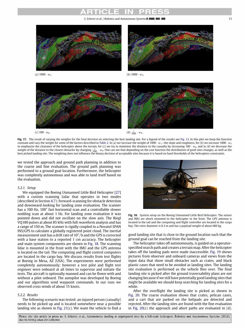
Fig. 10. Example point cloud showing terrain and power lines.

Fig. 11. Close-up of the sensor head mounted on the nose of the Unmanned LittleBird.


Fig. 12. The experimental setup for data collection on a EC 135 helicopter in Pittsburgh, PA, USA. We mounted a lidar, and inertial navigation system on a helicopter asshown in (a). The sensor platform is shown in (b). The inertial measurement unit was mounted next to the lidar to minimize errors in the registration of the data.

standard deviation σc and the altitude difference between themean of neighboring cells1µc = maxn∈Neighbors(c)(|µc − µn|). Thecost is calculated as follows

Cground =

max(σscale(σc − σmin)), 1µscale(1µc − 1µmin)∞ if Known Obstacle. (29)

The cost-to-go is then repeatedly computed using a dynamic-programming wavefront algorithm [25] from the ground goallocation pgoal up to amaximum cost-to-go thatwe consider. In veryrough terrain or with lots of missing cells only short paths will begeneratedwhile on smooth terrain such as roads long pathswill befound which represents the time to traverse. The cumulative costis then used as another factor in the goodness evaluation.

4.5. Goodness assessment

Landing site selection is a problem where many factors needto be considered to evaluate the cost of a site. Depending onthe weights for the goodness calculation, different sites will bechosen as best sites. A linear combination of the factors describedin Table 2 is considered to calculate the goodness of a landing site.Currently we manually set the weights ω1, . . . , ω7 to determine agoodness.

4.6. Computational efficiency

A naive online implementation of the algorithms above will beinfeasible to evaluate in real-time. We parallelize and incremen-tally compute updates to enable a real-time implementation. Thefollowing techniques enable real-time computation on a multi-core processor:

• All trivial parallel evaluations are spread across multiple cores.This includes evaluating– the fine evaluation of a set of sites.– the detection if any landing approaches need to be recom-

puted.– a series of landing approach directions.

• A triangulation is only created if a fine evaluation is performedin that region.

• A fine evaluation is only performed if any of the rough terraincells change.

• Fine evaluations are performed radially outward from theground goal location pgoal. As computation time permits landingsites further and further away will be checked.

• An approach path is only evaluated if the terrain cells related toit have changed.

• Only a fixed number of approach and abort directions areevaluated.

Our current implementationwill use asmany cores as are availableand can use those cores efficiently. Using this approachwe are ableto calculate landing sites in real-time at normal helicopter speeds.

4.7. Perception system design

The sensing system for an unmanned platform operating in anunmapped environment must provide two types of information:terrain information for analysis of potential landing zones, andproximity information about obstacles it may encounter en-route.Many sensing modalities are available for both tasks, with varyingsuitability for each task. The driving requirement in our casewas high-resolution measurement of the terrain while flying ata reasonable speed and altitude for a full-scale helicopter. Thisterrain measurement requirement rules out radar and MachineVision. A radar sensor with sufficient angular resolution wouldrequire a large antenna, and the depth and angular resolutionof vision systems is inadequate except at close range. Recentadvances in scanning lidar technology have improved the rangeand bandwidth significantly, opening this modality as a primecandidate for a viable perception system on a full-scale helicopter(see Figs. 7 and 11).

We designed and built a 3-D scanning lidar that operates intwo modes: forward-scanning for obstacle detection during low-altitude flight (Fig. 8), and downward scanning for terrainmappingand landing zone search from a higher altitude (Fig. 9). The scanneroperates in two axes: a fast 100 Hz, 100° transverse scan and aslower ‘‘nodding’’ scan that cycles up and down. The fast-axis scanis provided off-the-shelf by the lasermanufacturer,while the slow-axis is a single-axis gimbal that we fabricated in-house. The lidarmeasures with a sampling frequency of 84 kHz, giving the pointdensity for a high-resolution terrain map. The sensor has a rangeof 150 m, centimeter accuracy, and can process multiple returnsfor obscurant and vegetation penetration. The laser is Class 1 andeye-safe andmore details about the specific model can be found inSection 5.2.1.

A critical parameter for continuous landing zone evaluation in aoverflight configuration is the ability to receive a sufficient densityof points to detect the smallest relevant obstacle (dsmallestobst).Given a lidar performance these parameters set speed (s) andaltitude limits (a) to achieve a sufficient point resolution on the


(a) Picture. (b) Input point cloud.

(c) Coarse evaluation.

(d) Fine evaluation.

Fig. 13. Results from the ‘‘three trees’’ area. (a) shows an aerial view of the scanned area and (b) shows the point cloud at the end of the scan.

ground to achieve detection. The speed is given by the scanfrequency:

s = dsmallestobst · f .

The altitude depends on the field of view and beam divergence

a = mindmax,

dsmallestobst

2 · αseparation − αdiv

and the point separation αseparation is a function of the number ofpoints given the measurements in a field of view:

αseparation =f · α

p.

For the analysis we used the following parameters f = 100 Hz,p = 85 000 Hz, dmax = 150 m, α = 100°, αdiv = 0.0171°, anddsmallestobst = 0.15 m. With these parameter we can fly at amaximum height of 58 m for a 15 cm obstacle and a speed

of 20 m/s (39 knots). This analysis assumes that there will only beone overflight.

The motion control for actuation of both axes is preciselysynchronized to a global timeframe so that for each measurement,the time is known and can be fused with INS data for pointregistration. Absolute encoders and a highly rigid frame allow thepointing angles to be known to < 0.01°.

The lidar is rigidly coupled to ahigh-accuracyGPS/INS systemsothat the attitude of the whole sensor head is precisely known at alltimes despite vibration. Otherwise, themapwill become ‘‘blurred’’due to errors in the measurement of where the instrument waspointed when each point was measured. Each measured point isregistered into a global reference frame. The INS uses a ring-lasergyro with< 10°/h drift, differential GPS with 1 cm accuracy, and aKalman filter that timestamps themeasurements into a timeframethat is synchronizedwith the rest of the perception and computingsystem.





Fig. 14. Results from the ‘‘sloped field’’ area.

The system was shown to be capable of detecting chain linkfences, wires (Fig. 10), and 4 in flat pallets (Fig. 19(d)) duringflight on a helicopter. Maps built without differential GPS arestill locally consistent after one map-building run, but possiblyinconsistent over time. In our experiments, we operate with1-centimeter differential GPS, but the maps would still have hadsufficient local consistency to pick up small obstacles, even if theiractual registered position was slightly off. This sensor was used inthe experiments in Section 5.2.

Even though the inertial navigation system we are using has ahigh accuracy it is not sufficient to register the points with highenough accuracy to evaluate landing sites in front of the helicopterat the glide slope, because the smallest potentially lethal obstaclewe consider is the height of a rail (15 cm). One could apply scanmatching techniques such as the one proposed by Thrun et al. [26]to smooth the matching of adjacent scans.

5. Experiments

We present two experimental results in this section. Thefirst set of results evaluates only the coarse and fine landingsite evaluation algorithm in a variety of different urban andvegetated environments. The second set of results demonstrates

the autonomous landing of the Boeing Unmanned Little Bird (ULB)helicopter in an unknown environment that includes ground pathplanning, and approach path generation.

5.1. Fine and coarse landing zone evaluation

In this sectionwe showresults for the coarse and fine evaluationbased on 3D point cloud datasets we collected. In these resultswe assume a straight line path from the landing site to a groundgoal location. The results are shown for natural and man-madeenvironments to illustrate several environments and varying costweights. For all the results in this section we used the sameparameter values for all experiments except in the case where weintentionally varied the values to demonstrate the influence on thesite chosen.

5.1.1. SetupFor our first experiment we collected point cloud datasets at

various locations around Pittsburgh, PA, USA. We overflew theareas in approximately straight lines with speeds between 10 and20 knots. On the bottom of the helicopter we mounted a laserscanner, inertial navigation system, and a documentation camera





Fig. 15. Results from the ‘‘wooded intersection’’ area.

(see Fig. 12). The Riegl LMS-Q140i-60 scans a line perpendicular tothe flight direction at 8000 points per second. The scan frequencyof the lidar is 60 Hz. The data are fused by a Novatel SPANINS/GPS to calculate a globally registered point cloud. The inertialmeasurement unit has a drift rate of 10°/h (0.02° reportedaccuracy) and the GPS is correctedwith a base station to a reported1 cmaccuracy. In totalwe collected data on9 siteswith a flight timeof 8 h. We discuss results from three representative sites.

The coarse evaluation is robust to errors in z since it performsa least squares fit to determine the slope. The fine evaluationrelies on a good point cloud registration and is not robustto misregistered points. Nevertheless, other methods exist toimprove point cloud registration to get a better input point cloudfrom lower performance INS systems.

5.1.2. ResultsThe first sitewas scanned at an altitude of about 100m (Fig. 13).

It is a field, and our ground goal point is located next to the slopeon the hill (see Fig. 13(d) for exact goal location). The result showsthe coarse and fine evaluation of landing sites in the environment.Several possibly good landing sites in the coarse evaluation arerejected in the fine evaluation phase. Finally, the best landing site

is picked in a spot with small slope and a large clearance fromobstacles.

In the ‘‘sloped field’’ dataset (Fig. 14) we have a slightly morecomplex scenario because a lot of landing sites exist and wemust choose a best one. Also a large number of smooth slopesneed to be rejected based on the plane fitting. The next dataset(Fig. 15) is very constrained and a possible landing site needs tobe chosen that still fulfills all the constraints. We also scanned thisdataset at an altitude of about 100 m. Just based on the coarseevaluation one can see that most points are not suitable and onlya small area exists that can be considered suitable for landing. Inthe fine evaluation some too optimistic locations from the coarseevaluation are rejected. The main reason for the rejection is thatthe landing gears cannot be placed successfully. After evaluatingthe cost a point in the middle of the open area that is closer to theground goal location is picked.

While the previous dataset was mostly in vegetated terrain wealso collected a dataset at a coal power plant (Fig. 16) at 150 melevation above ground. The geometry of obstacles at the powerplant is very different from vegetation, but the algorithm is stillable to determine good landing sites. The ground goal location isclose to a car, and one can see how the fine evaluation rejects the





Fig. 16. Results from the ‘‘power plant’’ area.

car and the red region around the ground goal. The red region is asafety buffer that prevents landing directly on top of the groundgoal. The overflight and real-time evaluation of landing sites isshown at http://youtu.be/IXbBNyt6tz4.

As a final experiment, we varied the weights for our evaluationfunction for four different parameters in the same terrain (Fig. 17).First we changed the weight for slope and roughness (Fig. 17(a)).Compared to the nominal evaluation, one can see that we nowchoose a landing site further away from the ground goal pointbecause it is in smoother and less sloped terrain. A similar locationis chosen in Fig. 17(b); however, since we try to emphasize thevolume of the underbody, the shape of the LZ is actually moreconvex than the evaluation in Fig. 17(a).

If we give a large weight to the distances to the casualty, weexpect the distance to be small. We can see in the evaluation forFig. 17(c) that far points have low weight and close points havethe lowest weight. In Fig. 17(d), the result is almost the same asFig. 17(c), except that now points close to the boundary also have alow value. Varying the weights, one notices that the weight vectorhas a large influence on the resulting chosen landing site.

5.2. Landing the unmanned Little Bird helicopter

In the previous section we presented landing site evaluationresults in a large variety of terrain around Pittsburgh, PA. In thissection we present results from Mesa, AZ. In this environment

http://youtu.be/IXbBNyt6tz4


(a) 1000 · w1 . (b) 1000 · w3 .

(c) 100 · w6 . (d) 11000 · w4 .

Fig. 17. The result of varying the weights for the final decision on selecting the best landing site. For a legend of the results see Fig. 13. In this plot we keep the functionconstant and vary the weight for some of the factors described in Table 2. In (a) we increase the weight of 1000 · w1—the slope and roughness, for (b) we increase 1000 · w3to emphasize the clearance of the helicopter above the terrain, for (c) we try to minimize the distance to the casualty by increasing 100 · w6 , and in (d) we decrease theweight of the distance to the closest obstacles by changing 1

1000 · w4 . One can see that depending on the cost function the distribution of good sites changes, as well as thebest picked landing site. The weighting does not influence the binary decision of acceptable sites because it is based on hard thresholds of the helicopters constraints.

we tested the approach and ground path planning in addition tothe coarse and fine evaluation. The ground path planning wasperformed to a ground goal location. Furthermore, the helicopterwas completely autonomous and was able to land itself based onthe evaluation.

5.2.1. SetupWe equipped the Boeing Unmanned Little Bird Helicopter [27]

with a custom scanning Lidar that operates in two modes(described in Section 4.7): forward-scanning for obstacle detectionand downward-looking for landing zone evaluation. The scannerhas a 100 Hz, 100° fast horizontal scan and a controllable slowernodding scan at about 1 Hz. For landing zone evaluation it waspointed down and did not oscillate on the slow axis. The RieglVQ180 pulses at about 85 kHzwith full-waveform analysis and hasa range of 150 m. The scanner is rigidly coupled to a Novatel SPANINS/GPS to calculate a globally registered point cloud. The inertialmeasurement unit has a drift rate of 10°/h and the GPS is correctedwith a base station to a reported 1 cm accuracy. The helicopterand main system components are shown in Fig. 18. The scanninglidar is mounted in the front with the IMU and the GPS antennais located on the tail. The computing and flight control computersare located in the cargo bay. We discuss results from test flightsat Boeing in Mesa, AZ (USA). The experiments were performedcompletely autonomously; however a test pilot and flight testengineer were onboard at all times to supervise and initiate thetests. The aircraft is optionally manned and can be flown with andwithout a pilot onboard. The autopilot was developed by Boeingand our algorithms send waypoint commands. In our runs weobserved cross winds of about 15 knots.

5.2.2. ResultsThe following scenario was tested: an injured person (casualty)

needs to be picked up and is located somewhere near a possiblelanding site as shown in Fig. 21(c). We want the vehicle to find a

Fig. 18. System setup on the Boeing Unmanned Little Bird Helicopter. The sensorand IMU are shock mounted to the helicopter in the front. The GPS antenna islocated in the tail and the computing and flight controller are located in the cargobay. The rotor diameter is 8.3 m and has a payload weight of about 680 kg.

good landing site that is close to the ground location such that theground goal can be reached from the landing site.

The helicopter takes off autonomously, is guided on a operator-specified searchpath and creates a terrainmap. After thehelicoptertakes off the landing pads were made inaccessible. Fig. 19 showspictures from observer and onboard cameras and views from theinput data that show small obstacles such as crates, and blackplastic cases that need to be avoided as landing sites. The landingsite evaluation is performed as the vehicle flies over. The finallanding site is picked after the ground traversability plans are notchanging because ifwe still have potentially good landing sites thatmight be available we should keep searching for landing sites for awhile.

After the overflight the landing site is picked as shown inFig. 20. The coarse evaluation shows that crates, pelican cases,and a cart that are parked on the helipads are detected andrejected. After the landing sites are found with the fine evaluationin Fig. 20(c) the approach and abort paths are evaluated in (d).


Fig. 19. The problem setup and input sample data. In (a) one can see the straight line search path that was performed to look for landing sites. A ground goal was given bya ‘‘casualty’’ that needs to be picked up. In (b) one can see a downward looking view from the helicopter looking at some obstacles on the runway. (c) shows an exampleobstacle and (d) shows a set of obstacles. (d) shows the correlation between obstacles (pallets, and plastic storage boxes) and the point cloud which is the input to thealgorithm. The data was collected at 40 knots from 150 ft AGL.

The path to the ground goal is shown in (e). A video that showsone of the landing site search and landing runs is available athttp://youtu.be/BJ3RhXjucsE.

From the parameters of the lowest cost landing site an approachpath is computed and sent to the vehicle. On this trajectory thevehicle turns around and descends at the desired sink rate andcomes to a hover about 3 m above the ground. After coming to ahover the vehicle orients itself to the optimal heading and thenexecutes a touchdown. Part of the final approach segment is shownin Fig. 21 where the helicopter is close to the final landing site. Thefirst view is a cockpit view of the clutter on the runway and vehicleon its way down to land. The second view shows the selected finallanding site and other potential sites to land. The last picture showsthe helicopter and the location of the ground goal. After a stablehover is achieved above the final goal location the vehicle touchesdown at the landing site.

After system integration and testing runs, a total of 8 landingmissions were demonstrated with varying ground clutter andapproach directions. Fig. 22 shows two typical landing missions.After an autonomous takeoff and climb out, the aircraft approachesthe flight line from the south-west. It overflies the landing areaat 40 knots and 150 ft AGL to search for acceptable landing sites.The computation time for landing zone evaluation is low enoughthat the vehicle can pick landing zones, and approach paths in real-time. The point cloud, aerial image and resulting path are shown inFig. 22 for two typical missions. The approach cost ω6 was varied

between Fig. 22(a) and (b) to penalize for an unknown approachcost.

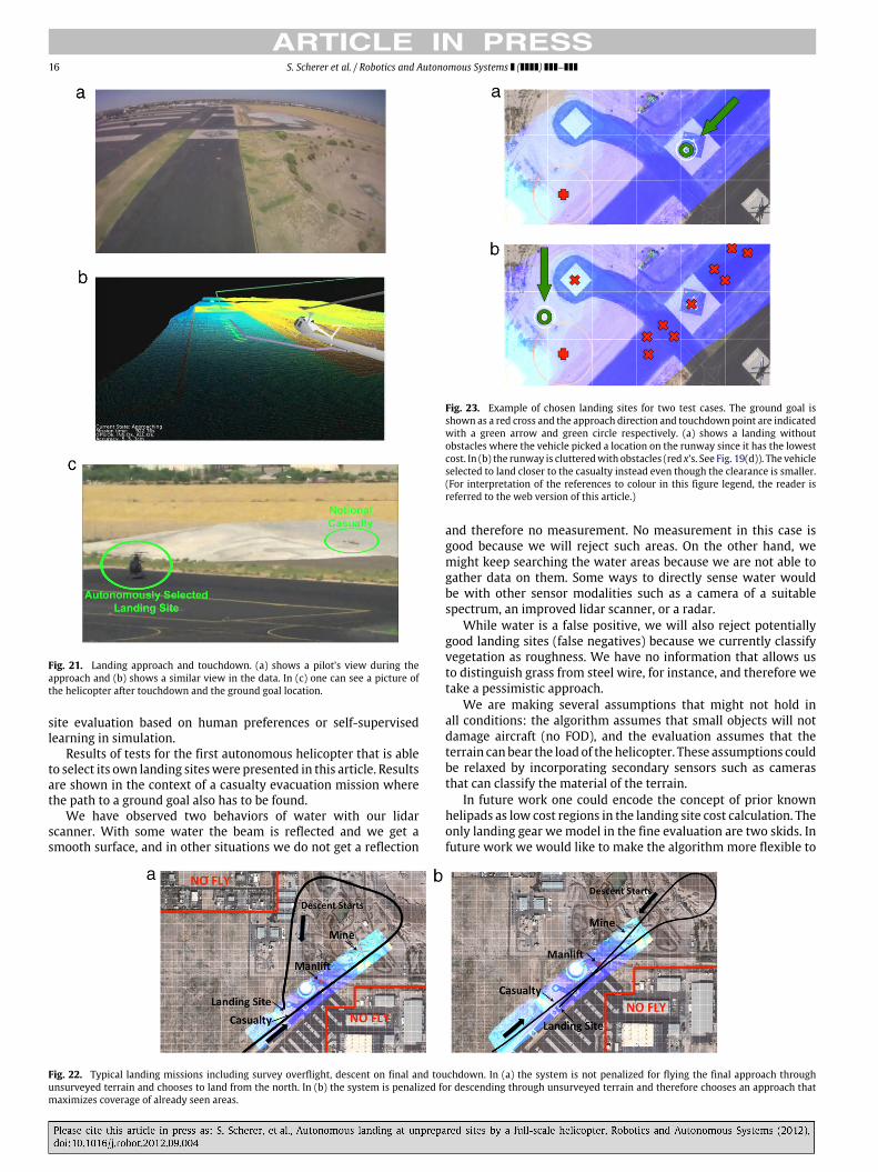
A close-up of twomissions flownwith a lowω6 (approach cost)weight are shown in Fig. 23. Since no obstacles are present inFig. 23(a) the vehicle prefers a landing site on the runway sinceit is a wide open area with a low landing site cost. As we clutteredthe runway Fig. 23(b) the vehicle instead now prefers a closer sitewith a shorter path. This result was unexpected since we expectedthe vehicle to land on the runway instead because there was a no-fly zone to the north. However, the approach it found went east ofthe no-fly zone and landed in a feasible location.

In the next two experiments the approach cost weight wasincreased (Fig. 24). This did not change the outcome of landingwithout obstacles since it also previously landed on the runway.In the case of obstacle clutter however the vehicle now preferredan approach that flew over the scanned area. Since most of theobstacles were low it was able to overfly the obstacles beforelanding.

Table 3 shows the computation times for the optimizedalgorithms that minimize re-computation of new data. Thecomputation was performed onboard with Intel 2.6 GHz Core 2Quad computers Adding new data is fast and takes currently about17 ms/100000 points which is much faster than real-time. Thecoarse evaluation is very fast at 699 ms/100000 cells. The fineevaluation is much slower which justifies the coarse evaluationto limit the number of fine evaluations performed. Approachevaluation also requires many evaluations and is therefore slower.

http://youtu.be/BJ3RhXjucsE


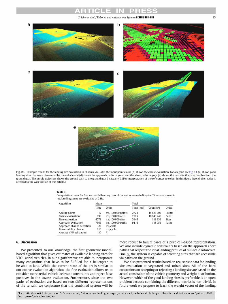
Fig. 20. Example results for the landing site evaluation in Phoenix, AZ. (a) Is the input point cloud. (b) shows the coarse evaluation. For a legend see Fig. 13. (c) shows goodlanding sites that were discovered by the vehicle and (d) shows the approach paths in green and the abort paths in grey. (e) shows the best site that is accessible from theground goal. The purple trajectory shows the ground path to the ground goal (‘‘casualty’’). (For interpretation of the references to colour in this figure legend, the reader isreferred to the web version of this article.)

Table 3Computation times for five successful landing runs of the autonomous helicopter. Times are shown inms. Landing zones are evaluated at 2 Hz.

Algorithm Mean TotalTime Units Time (ms) Count (#) Units

Adding points 17 ms/100000 points 2723 15826707 PointsCoarse evaluation 699 ms/100000 cells 7575 10843248 CellsFine evaluation 4578 ms/100000 sites 5446 118951 SitesApproach evaluation 7663 ms/100000 paths 9116 118951 PathsApproach change detection 21 ms/cycleTraversability planner 113 ms/cycleAverage CPU utilization 30 %

6. Discussion

We presented, to our knowledge, the first geometric model-based algorithm that gives estimates of available landing sites forVTOL aerial vehicles. In our algorithm we are able to incorporatemany constraints that have to be fulfilled for a helicopter tobe able to land. While the current state of the art is similar toour coarse evaluation algorithm, the fine evaluation allows us toconsider more aerial-vehicle-relevant constraints and reject falsepositives in the coarse evaluation. Furthermore, since the twopaths of evaluation are based on two different representationsof the terrain, we conjecture that the combined system will be

more robust to failure cases of a pure cell-based representation.We also include dynamic constraints based on the approach abortpaths that respect the ideal landing profiles of full-scale rotorcraft.Finally, the system is capable of selecting sites that are accessiblevia paths on the ground.

We also presented results based on real sensor data for landingsite evaluation at vegetated and urban sites. All of the hardconstraints on accepting or rejecting a landing site are based on theactual constraints of the vehicle geometry andweight distribution.However, which of the good landing sites is preferable is an openproblem because combining the different metrics is non-trivial. Infuture work we propose to learn the weight vector of the landing


Fig. 21. Landing approach and touchdown. (a) shows a pilot’s view during theapproach and (b) shows a similar view in the data. In (c) one can see a picture ofthe helicopter after touchdown and the ground goal location.

site evaluation based on human preferences or self-supervisedlearning in simulation.

Results of tests for the first autonomous helicopter that is ableto select its own landing siteswere presented in this article. Resultsare shown in the context of a casualty evacuation mission wherethe path to a ground goal also has to be found.

We have observed two behaviors of water with our lidarscanner. With some water the beam is reflected and we get asmooth surface, and in other situations we do not get a reflection

Fig. 23. Example of chosen landing sites for two test cases. The ground goal isshown as a red cross and the approach direction and touchdown point are indicatedwith a green arrow and green circle respectively. (a) shows a landing withoutobstacles where the vehicle picked a location on the runway since it has the lowestcost. In (b) the runway is clutteredwith obstacles (red x’s. See Fig. 19(d)). The vehicleselected to land closer to the casualty instead even though the clearance is smaller.(For interpretation of the references to colour in this figure legend, the reader isreferred to the web version of this article.)

and therefore no measurement. No measurement in this case isgood because we will reject such areas. On the other hand, wemight keep searching the water areas because we are not able togather data on them. Some ways to directly sense water wouldbe with other sensor modalities such as a camera of a suitablespectrum, an improved lidar scanner, or a radar.

While water is a false positive, we will also reject potentiallygood landing sites (false negatives) because we currently classifyvegetation as roughness. We have no information that allows usto distinguish grass from steel wire, for instance, and therefore wetake a pessimistic approach.

We are making several assumptions that might not hold inall conditions: the algorithm assumes that small objects will notdamage aircraft (no FOD), and the evaluation assumes that theterrain canbear the loadof thehelicopter. These assumptions couldbe relaxed by incorporating secondary sensors such as camerasthat can classify the material of the terrain.

In future work one could encode the concept of prior knownhelipads as low cost regions in the landing site cost calculation. Theonly landing gear wemodel in the fine evaluation are two skids. Infuture work we would like to make the algorithm more flexible to

Fig. 22. Typical landing missions including survey overflight, descent on final and touchdown. In (a) the system is not penalized for flying the final approach throughunsurveyed terrain and chooses to land from the north. In (b) the system is penalized for descending through unsurveyed terrain and therefore chooses an approach thatmaximizes coverage of already seen areas.


Fig. 24. Example of chosen landing sites with the system preferring knownapproach directions. In (a) the system selects a site on the runway that is reachablewith a low-cost path the site selected is similar to Fig. 23(a). In (b) the vehicle willstill prefer an approach through measured terrain. It picks a landing zone that ison the runway further away from the ground goal since it is the only clear areathat has an obstacle clear glide slope. The area close to the ground goal is free andclear; however it is not chosen as a landing site since a hill (bright area in lower-left)increases the approach cost and the approach is not known to be free.

be applicable to different kinds of landing gear and test in morechallenging environments.

Acknowledgments

Our team would like to thank TATRC (Telemedicine andAdvanced Research Center) from the US Army Research andMateriel Command for funding this research. Our thanks go to ourpartners at Piasecki Aircraft Corp, whose expertise and financialcommitment allowed us to test on a full-scale vehicle. The BoeingCompany provided use of the Unmanned Little Bird and the testfacilities in Mesa, AZ.We thank the ULB flight test team for makingthe integration and testing a safe and productive experience.

References

[1] F. Harris, E. Kasper, L. Iseler, US civil rotorcraft accidents, 1963 through 1997,Tech. Rep. NASA/TM-2000-209597, NASA, 2000.

[2] F. Kendoul, Survey of advances in guidance, navigation, and control ofunmanned rotorcraft systems, Journal of Field Robotics 29 (2) (2012) 315–378.

[3] J. Sprinkle, J. Eklund, S. Sastry, Deciding to land a UAV safely in real time,in: Proceedings of the American Control Conference, ACC, vol. 5, 2005, pp.3506–3511.

[4] S. Saripalli, G. Sukhatme, Landing a helicopter on a moving target, in:Proceedings IEEE International Conference on Robotics and Automation, 2007,pp. 2030–2035.

[5] D. Barber, S. Griffiths, T. McLain, R.W. Beard, Autonomous landing ofminiatureaerial vehicles, in: Proceedings of the AIAA Infotech@Aerospace Conference,2005.

[6] C. de Wagter, J. Mulder, Towards vision-based UAV situation awareness, in:Proceedings of the AIAA Conference on Guidance, Navigation, and Control,GNC, 2005.

[7] Z. Yu, K. Nonami, J. Shin, D. Celestino, 3D vision based landing control of asmall scale autonomous helicopter, International Journal of Advanced RoboticSystems 4 (1) (2007) 51–56.

[8] L. Mejias, P. Campoy, K. Usher, J. Roberts, P. Corke, Two seconds totouchdown-vision-based controlled forced landing, in: Proceedings of theIEEE/RSJ International Conference on Intelligent Robots and Systems, 2006, pp.3527–3532.

[9] J. Hintze, Autonomous landing of a rotary unmanned aerial vehicle in anon-cooperative environment usingmachine vision, Master’s Thesis, BrighamYoung University.

[10] S. Bosch, S. Lacroix, F. Caballero, Autonomous detection of safe landingareas for an UAV from monocular images, in: Proceedings of the IEEE/RSJInternational Conference on Intelligent Robots and Systems, 2006, pp.5522–5527.

[11] A. Johnson, J. Montgomery, L. Matthies, Vision guided landing of an au-tonomous helicopter in hazardous terrain, in: Proceedings IEEE InternationalConference on Robotics and Automation, 2005, pp. 3966–3971.

[12] J.F. Montgomery, A.E. Johnson, S.I. Roumelliotis, L.H. Matthies, The jet propul-sion laboratory autonomous helicopter testbed: a platform for planetary ex-ploration technology research and development, Journal of Field Robotics 23(2006) 245–267.

[13] T. Templeton, D. Shim, C. Geyer, S. Sastry, Autonomous vision-based landingand terrain mapping using an MPC-controlled unmanned rotorcraft, in:Proceedings IEEE International Conference on Robotics and Automation, 2007,pp. 1349–1356.

[14] M. Sanfourche, G. le Besnerais, P. Fabiani, A. Piquereau, M. Whalley,Comparison of terrain characterization methods for autonomous UAVs, in:Proceedings of the 65th Annual Forum of the American Helicopter Society,Grapevine, TX, 2009.

[15] M.Whalley, M. Takahashi, G. Schulein, C. Goerzen, Field-testing of a helicopterUAV obstacle field navigation and landing system, in: Proceedings of the 65thAnnual forum of the American Helicopter Society, AHS, Grapevine, TX, 2009.

[16] M. Takahashi, A. Abershitz, R. Rubinets, M. Whalley, Evaluation of safelanding area determination algorithms for autonomous rotorcraft using sitebenchmarking, in: Proceedings of the 67th Annual forum of the AmericanHelicopter Society, AHS, Virginia Beach, VA, 2011.

[17] N. Serrano, A Bayesian framework for landing site selection during au-tonomous spacecraft descent, in: Proceedings of the IEEE/RSJ InternationalConference on Intelligent Robots and Systems, 2006, pp. 5112–5117.

[18] B. Sofman, J. Bagnell, A. Stentz, N. Vandapel, Terrain classification from aerialdata to support ground vehicle navigation, Tech. Rep. CMU-RI-TR-05-39, TheRobotics Institute, Carnegie Mellon University, Pittsburgh, PA, 2006.

[19] M. Hebert, N. Vandapel, Terrain classification techniques from ladar datafor autonomous navigation, in: Proceedings of the Collaborative TechnologyAlliances Conference, 2003.

[20] B. Welford, Note on a method for calculating corrected sums of squares andproducts, Technometrics 4 (3) (1962) 419–420.

[21] T. Templeton, Autonomous vision-based rotorcraft landing and accurate aerialterrain mapping in an unknown environment, Tech. Rep. USB/EECS-2007-18,University of California at Berkeley, Berkeley, CA, 2007.

[22] S. Joon Ahn, Least Squares Orthogonal Distance Fitting of Curves and Surfacesin Space, in: Lecture Notes in Computer Science, Springer, 2005.

[23] F. Preparata, M. Ian Shamos, Computational Geometry: An Introduction,Springer, 1985.

[24] A. Fabri, G. Giezeman, L. Kettner, S. Schirra, S. Schönherr, The CGAL Kernel: abasis for geometric computation, in:M.C. Lin, D.Manocha (Eds.), Proc. 1st ACMWorkshop on Appl. Comput. Geom., in: Lecture Notes Comput. Sci., vol. 1148,Springer-Verlag, 1996, pp. 191–202.

[25] H. Choset, K.M. Lynch, S. Hutchinson, G. Kantor, W. Burgard, L.E. Kavraki, S.Thrun, Principles of Robot Motion: Theory, Algorithms, and Implementations,The MIT Press, 2005.

[26] S. Thrun, M. Diel, D. Hahnel, Scan alignment and 3-D surface modeling with ahelicopter platform, in: Proceedings of the International Conference on Fieldand Service Robotics, 2003.

[27] Boeing, http://www.boeing.com/rotorcraft/military/ulb, 2010.

Sebastian Scherer is a Systems Scientist at the RoboticsInstitute (RI) at Carnegie Mellon University (CMU). Hisresearch focuses on enabling unmanned rotorcraft tooperate at low altitude in cluttered environments. He hasdeveloped a number of intelligent autonomous rotorcraft.Dr. Scherer received his B.S. in computer science, and hisM.S. and Ph.D. in robotics from CMU in 2004, 2007, and2010.

http://www.boeing.com/rotorcraft/military/ulb


Lyle Chamberlain is a Sensor Hardware Engineer at theRobotics Institute at Carnegie Mellon University. His workhas focused on bringing robot perception technology tothe world of flying vehicles, both large and small. Mr.Chamberlain received a B.S. in engineering and appliedscience from the California Institute of Technology in 2005.

Sanjiv Singh is a Research Professor at the RoboticsInstitute at Carnegie Mellon University. His researchrelates to the operation of robots in natural and in somecases, extreme environments. Dr. Singh received his B.S. incomputer science from the University of Denver in 1983,his M.S. in electrical engineering from Lehigh Universityin 1985, and a Ph.D. in robotics from Carnegie MellonUniversity in 1995. He was a member of the research staffat the Robotics Institute from 1985 to 1989. He was aPostgraduate Fellow at Yale University in 1990 and anNSF Fellow at the Mechanical Engineering Laboratory in

Tsukuba, Japan in 1992.

Documents

Paper - The Robotics Institute - Carnegie Mellon University