Technical Report EL-94-3February 1994

US Army Corps ( )of EngineersWaterways Experiment AD-A278 542Station oIlin mnmn

Environmental Impact Research Program

A Conceptual Frameworkfor the Evaluationof Coastal Habitats

by Gary L. RayEnvironmental Laboratory

DTICS ELECTES APR2Z5 1994D

Approved For Public Release; Distribution Is Unlimited

94-12416Il IIIII 111111111111111 l il Ul 11 lilt -+ , + +: • •

Prepared for Headquarters, U.S. Army Corps of Englnegrs.,

944X1

The contents of this report are not to be used for advertising,publication, or promotional purposes. Citation of trade namesdoes not constitute an official endorsement or approval of the useof such commercial products.

i Rw= ow ww= PAPI

Environmental Impact Technical Report EL-94-3Research Program February 1994

A Conceptual Frameworkfor the Evaluationof Coastal Habitatsby Gary L. Ray

Environmental Laboratory

U.S. Army Corps of EngineersWaterways Experiment Station3909 Halls Ferry RoadVicksburg, MS 39180-6199

Acceslon ForNTIS CRA&JDTIC TABUnannounced 13Justification

By.... ..Distribution I

Availability Codes

Avail and j orDist Special

Final reportAppoved for public release; distribution Is unlimited

Prepared for U.S. Army Corps of EngineersWashington, DC 20314-1000

US Army Corpsof EngineersWaterways Experiment

Waterways Experiment Siation Cataloging.In.Publication Data

Ray, Gary L.A conceptual framework for the evaluation of coastal habitats I by Gary L. Ray ;

prepared for U.S. Army Corps of Engineers.67 p. :1il. ; 28 cm. - (Technical report ; EL-94-3)Includes bibliographic references.1. Aquatic habitats - Evaluation. 2. Coastal ecology - Evaluation. 3. Habitat

(Ecology). 4. Esuarln ecology - Evaluation. I. Enviromental Impc Re-search Program (U.S.) II. United States. Army. Corps of Engineers. Ill. U.S.Army Engineer Waterways Expernment Station. IV, Title. V. Series: Technical re-port (U.S. Army Engineer Waterways Exerment Station) ; EL-94-3.TA7 W34 no.EL-94-3

INALM COSFAL OMO

MAIN 49OMW ON

Contents

Preface ................................................ iv

I-Introduction ......................................... 1

Problem Statement ...................................... 1A Conceptual Framework .................................. 3

2-Framework for a Coastal Habitat Evaluation Method .............. 6

Step 1. Identifying System Boundaries ........................ 6Step 2. General Background Data ........................... 7Step 3. Identifying Habitats ................................ 8

Existing coastal habitat classification schemes ................. 8Coastal habitat classification scheme ........................ 9Data necessary for identifying habitats ..................... 10

Step 4. Habitat Attributes ................................ 10Step 5. Regional Attribute Values .......................... 12Step 6. Habitat Mapping ................................. 13Step 7. Attribute Measures ............................... 14Step 8. Attributes in Relation to Expected Values ............... 15Step 9. Calculating Total System Attributes ................... 15Step 10. Comparison of System Attribute Totals ................ 15

3- Discussion ........................................... 17

References ............................................. 19

Figures 1-3

Tables 1-18

SF 298

|ii

Preface

This report was prepared by the Ecological Research Division (ERD), Envi-ronmental Laboratory (EL), U.S. Army Engineer Waterways Experiment Sta-tion (WES), as part of the Environmental Impact Research Program (EIRP),sponsored by Headquarters, U.S. Army Corps of Engineers (HQUSACE).Technical monitors were Dr. John Bushman and Mr. Frederick B. Juhle,HQUSACE. Dr. Roger T. Saucier, EL, WES, was EIRP Program Manager.

The framework is the result of the collaborative efforts of a multi-disciplinary working group that included Marcia Bowen (Normadeau Associ-ates, New Bedford, NH), Dr. Robert Diaz (Virginia Institute of MarineSciences, Glouster Point, VA), Dr. Courtney T. Hackney (Breedlove, Dennis &Associates, Orlando, FL), Dr. Mark LaSalle (Mississippi State UniversityCoastal Research and Extension Service, Biloxi, MS), Dr. Nancy Rabalais(Louisiana Universities Marine Consortium, Chauvin, LA), Mr. CharlesSimenstad (Fisheries Research Institute, University of Washington, Seattle,WA), and Dr. Douglas Clarke (WES).

The report was written by Dr. Gary L. Ray, ERD, EL, WES. Workprogressed under the general supervision of Mr. Edward J. Pullen, Chief,Coastal Ecology Branch, ERD; Dr. Conrad J. Kirby, Chief, ERD; and Dr. JohnHarrison, Director, EL.

At the time of publication of this report, Director of WES wasDr. Robert W. Whalin. Commander was COL Bruce K. Howard, EN.

This report should be cited as follows:

Ray, G. L. (1994). "A Conceptual framework for the evaluationof coastal habitats," Technical Report EL-94-3, U.S. Army Engi-neer Waterways Experiment Station, Vicksburg, MS.

iv

1 Introduction

Problem Statement

Mitigation for damage to estuarine and marine habitats by engineeringprojects often involves habitat restoration or replacement. Such activitiesgenerally require the sacrifice of a different habitat type. For instance, anoyster bed might be constructed by placement of shell (cultch) on nearbyunvegetated substrates. In this case, the unvegetated substrate habitat is tradedfor oyster-bed habitat. At other times, it may be impossible or impractical toconstruct or restore the original habitat type, and an "out-of-kind" habitat isconstructed. In the previous example, a seagrass bed might be constructed inlieu of oyster-bed habitat.

Evaluating the environmental impact of habitat "trade-offs" involves com-parison of both constructed or restored sites with natural habitats (e.g., a con-structed oyster bed versus a natural oyster bed) and disparate habitat types(e.g., oyster beds, grass beds, and unvegetated substrates). At first glance,such an analysis appears to be a classic case of comparing "apples andoranges." Downing (1991) explored this analogy and noted that apples,oranges, and any other set of objects (including habitats and ecosystems) canbe meaningfully compared if common features are examined. In the case ofhabitats or ecosystems, comparisons can be made using structural characteris-tics and ecological functions or attributes.

The biological structures characteristic of a habitat are the communities thatmake it up (Table 1). The ecological attributes are those functions providedby the habitat to the ecosystem as a whole (e.g., primary productivity andpredation refuges). A seagrass habitat can be used as an example; it consistsof rooted vascular plants, epiflora (diatoms and other flora that live on thegrass blades), sediment microflora (mostly diatoms), epifauna (e.g., amphi-pods), infauna (e.g., polychaetes), and fish and invertebrate populations thatspend part or all of their lives in the grassbed. The attributes provided by thishabitat include primary productivity of the seagrass and other floral communi-ties and secondary productivity of the faunal communities. The seagrassblades serve as substrate for attachment for sedentary species and for place-ment of eggs by motile species. The physical structure of the bed also

ChOter 1 Inoductdon

provides a refuge from predation for many organisms at different points intheir life histories.

An evaluation technique specifically designed to compare different habitatsshould measure a wide diversity of structures and functional attributes (LaSalleand Ray 1992). Measurement of primary production in the seagrass bed dis-cussed above can be used as an example of the complexity of this problem.Sources of primary production include vascular plants, algae, and diatoms.Each of these sources is associated with various structures in the environment(e.g., sediment, rocks, and vascular plant stems or leaves) and requires separateevaluation. The productivity of each source will ultimately produce differentquantities and qualities of food material for consumer species. Productivity ofeach source will also vary according to the location of the habitat within anindividual coastal system and over the habitat's geographical range. Bowenand Small (1992) reviewed evaluation techniques available for coastal habitatsand concluded that existing methods are inadequate. Methods such as theWetland Evaluation Technique (WET) (Adamus and Stockwell 1983; Adamuset al. 1987; Diaz 1982) and Benthic Resources Assessment Technique (Lunzand Kendall 1982) cannot be applied to all habitats and do not measure allimportant functional attributes. Likewise, the Habitat Evaluation Procedure(HEP) (U.S. Fish and Wildlife Service (USFWS) 1980) relies on Habitat Suit-ability Index models that have been difficult to devise for coastal species(Nelson 1987). The Biological Evaluation Standardized Technique (BEST)(MEC Analytical Systems, Inc. 1988) suffers from being driven by individualspecies requirements rather than habitat attributes. These techniques are alsoinadequate to evaluate the contribution individual habitats make to the func-tioning of other habitats in the ecosystem.

Individual habitats do not exist in isolation, but are interdependent parts ofcoastal ecosystems. For instance, seagrasses not only support habitat-specificflora and fauna, but also export detritus, which is used as food by other com-munities. Likewise, coastal organisms move freely from one habitat to thenext to satisfy their life history requirements for shelter, feeding, reproduction,and development. Habitat trade-offs result in a change in both the areal extentof certain habitats and the relative proportions of habitat types present in asystem. While the impact of an individual trade-off is generally minimal, aseries of trade-offs occurring over a number of years or in concert withimpacts from other sources (e.g., changes in land-use patterns) can result in asignificant change in the nature of a system. The depletion of wetlands inheavily industrialized estuaries is an extreme example of such a situation.While the importance of assessing the cumulative impact of changes in theamounts and proportions of habitats in a system is generally recognized, exist-ing evaluation methods do not deal with these problems. If the issue of habitattrade-offs is to be meaningfully addressed, new techniques need to be devised.A conceptual framework for one such technique is presented in this document.It was suggested by a working group of estuarine scientists and has beenbriefly described in LaSalle and Ray (1992).

2 Chapter 1 Introduction

A Conceptual Framework

As with any evaluative method, a new habitat comparison technique needsto be quantitative, repeatable, flexible, understandable on technical and non-technical levels, accurate, and cost-effective (Diaz 1982; Bowen and Small1992). A technique designed specifically to evaluate habitat trade-offs mustadditionally examine a broad range of structural and functional attributes,compare values for these attributes with those expected in the appropriategeographic region, and provide a mechanism for interpreting changes in theseattributes on a system-wide basis. Comparisons should also be made on asystem-by-system basis because each watershed, estuary, or coastline is charac-terized by a unique combination of geological, morphological, hydrodynamic,and meteorological features. These elements interact to determine the basictypes, area, and quality of habitats that are present at any given time. It isassumed that each coastal system will potentially support a particular range ofhabitats in system-specific proportions and, therefore, must be analyzedindividually.

The framework described in this document is essentially an inventory andaccounting procedure that utilizes habitat attributes as basic input. Habitats ina system (e.g., estuary, watershed, and area of coastline) are mapped and theirareas measured. Their structural and functional attributes are then listed, andan estimate is made of the extent to which each habitat attains the valueexpected for that region of the country. For instance, the benthic algal primaryproductivity of a specific mud flat in Virginia may only achieve 75 percent ofwhat is normal for that region while another mud flat in the same system mayrealize 100 percent of the expected productivity. These percentages are thenmultiplied by the area of the habitat to arrive at a habitat/attribute value. If thefirst mud flat has an area of 50 ha, its habitat/attribute value would be 0.75times 50 or 37.5 units. If the area of the second mud flat is also 50 ha, itwould have a value of 1.00 times 5J or 50 units. This process is repeated foreach habitat-attribute combination, and values for identical habitats aresummed. In the previous example, the total mud flat benthic primary produc-tivity value for that system would be 87.5 units. The 87.5-unit value can thenbe compared with estimates of historical conditions to evaluate how the systemhas changed, or used as a baseline for with-project and without-projectcomparisons.

At this point, it is important for the reader to recognize that the frameworkdescribed in this document is still in a formative stage. Many of its underlyingassumptions have not been rigorously tested, and case studies are just gettingunderway. Enhancement and refinement of the basic procedure will berequired as the validity of the underlying assumptions are examined and practi-cal experience is gained.

In subsequent sections, the steps necessary to perform the analysis arediscussed and demonstrated using a hypothetical system. The procedure itselfcan be broken down into 10 steps (Table 2). The first step is to define theboundaries of the system under study. Next, background information on the

3C~hapla I Inatroucion

system is collected and compiled. The background information itself consistsof two types: data necessary for an understanding of the general nature of thesystem (e.g., hydrodynamics and meterology), and data used directly in theanalysis (e.g., estimates of primary production by seagrasses and fisheriesutilization of benthic invertebrates). Habitats present in the system are identi-fied (Step 3) along with their critical attributes (Step 4). Fifth, the averageattribute values expected in that region of the country are established fromliterature sources. Sixth, habitats are mapped and the area of each habitat typeis measured. Seventh, an estimate or direct measure of each attribute (e.g.,mud flat benthic invertebrate production) is then made and compared with theregional average. So that these values are understandable by nonexperts, theattribute is expressed as a percentage of the regional average (Step 8). Ninth,as previously described, the attribute value is multiplied by the area of thehabitat to produce a value that represents the total amountof a particular attri-bute that is supplied to the system. Finally, the total amount of each habitat'sattributes are compared for different time periods (e.g., historical versus presentconditions) or different scenarios (e.g., with and without project conditions).

The advantage of this framework is that it clearly identifies probable lossesand gains because of changes in the habitats in a system. The tendency toequate innately different attribute types (seagrass primary production versussalt marsh primary production) is avoided because each attribute is identifiedas a separate entity.

The framework uses both qualitative (habitat type) and quantitative (habitatattribute) data and should be cost-effective in that much of the raw data for thecalculations is already available from the technical literature or governmentpublications. The calculations are simple enough to be performed with virtu-ally any computer spreadsheet program. The procedure is flexible since it isindependent of the types of habitats or environmental status (e.g., polluted andpristine) of the system to which it is applied. It is also "upgradable" in iOhesense that as new information is obtained, it can be entered into the calcula-tions with minimal effort. The results of the calculations are sufficiently intui-tive to be understood on the nontechnical level, yet provide adequateinformation for making technically based decisions. Also, the results provideinformation for the decision-making process but do not drive that process.This problem is inherent in species-based evaluation methods such as HEP orBEST, where the choice of target species injects bias.

The combination of a system-wide and system-by-system analysis makesthis approach fundamentally different from the current practice of project-specific analysis. The new framework will require a substantial change fromcurrent approaches to evaluating impacts to habitats. Under the project-specific approach, a relatively small amount of information is evaluated duringa project, but the entire process must be repeated every time there is a newproject. This repetition results in a considerable amount of wasted time andeffort. In addition, changes in personnel or simply the passage of time canlead to inconsistent results by application of different standards. The system-wide approach requires that a broad-based and long-term perspective be taken

4 Chapter I Introducton

towards project evaluations. The assembly of background data, mapping ofhabitats, and assignment of expected attribute values for an entire system willnot be a trival effort. The initial investment, however, should be repaid byeliminating the repetition of effort associated with the project-specificapproach. Finally, decision-making processes will be improved, because thechoices inherent in implementing the framework (e.g., the initial choice ofcritical attributes and the assessment of what changes in these variables mayimply) require a consensus among decision-makers regarding the importance ofspecific attributes, the environmental status of the system, and the ultimateenvironmental goals for the system.

5ChapWr I Inoduclion

2 Framework for a CoastalHabitat Evaluation Method

Step 1. Identifying System Boundaries

The first step in the framework is to establish the boundaries of the systemto be studied (Table 2). Upland limits are the maximum extent of the water-shed or drainage basin. In large systems, multiple watersheds may beinvolved. The upland limits are not used directly in subsequent analyses, butprovide a logical boundary for assessing the character and environmental statusof the system. For instance, knowledge of land-use patterns in upland areas(e.g., industrial or urban development, agricultural practices, and natural uplandhabitats) is needed to understand potential sources of disturbance (e.g., point ornonpoint pollution sources). Coastal watershed and drainage basin boundarieshave been mapped in most areas of the country and can be found in theNational Oceanographic and Atmospheric Administration (NOAA) NationalEstuarine Inventory Data Atlas (NOAA 1985) or the United States GeologicalSurvey's Hydrological Unit Maps. The National Esmarine Inventory mapsalso include basic data on total surface area, area of salinity zones, drainagebasin shape, freshwater inflow rates, prevailing tides, tidal ranges, position oftide gauges, and cross-sectional topographic profiles.

Boundaries for the delineation of habitats in the system are the terrestrial,aquatic, and seaward limits. The terrestrial limit is the uppermost extent of theintertidal zone and can be determined from surface elevations and tidal rangesor from vegetational patterns. NOAA is presently mapping the coastal marshesof the United States, and these maps will be the most efficient source of infor-mation since it will be possible to simultaneously determine the terrestrialboundary and marsh and intertidal habitat areas. The aquatic limit is the maxi-mum extent of tidal influence in associated rivers and can be deduced fromtidal charts or vegetation patterns. Establishing the seaward boundary of asystem is more problematic. Few precise boundaries analogous to the water-shed exist, and those that do (e.g., the limits of the Continental Slope), do notimpose a physical barrier to the exchange of material, energy, or organisms.Geographic variation also makes generalization difficult. The difficulty indefining the seaward boundary makes it necessary to arbitrarily define it as themaximum extent of estuarine influence. This boundary obviously limits initial

6 Chapter 2 Framework tor a Coastal Habitat Evaluation M'etod

applications to estuaries. However, this is a reasonable restriction since mosttrade-offs involve estuarine habitats. Appropriate boundaries for purely marineor marine-estuarine systems will be developed at a later time.

To illustrate the identification of boundaries and all subsequent steps, ahypothetical system, "Anywhere Bay," will be analyzed. A map of the bay ispresented in Figure 1. Upland limits of the system are indicated by the water-shed. The landward system boundary was estimated from aerial photographs,and the seaward limits were derived from a National Estuarine Inventory Map.The system is comprised of nine different habitat types occurring in variousamounts (Table 3). Figure 2 presents the distribution of each habitat type.The example scenario is that a development is planned in the upper reaches ofthe estuary. Approximately 800 ha of oligohaline marsh will be directly elimi-nated and 100 ha of polyhaline seagrass planted on previously unvegetatedsands as mitigation. Figure 3 depicts the system after both development andhabitat construction activities have occurred.

Step 2. General Background Data

A variety of data types will be necessary for the development of the infor-mation database. Much of this information will not be used directly in theanalysis, but is essential to understand the specific nature of the system(Table 4). These data include descriptions of the system's physiography, geol-ogy, climate, water quality, and hydrodynamics. Particularly useful summariescan be found in the "Ecological Characterization" publications of the U.S. Fishand Wildlife Service (e.g., Fefer and Schettig 1980). These reports cover mostof the major regions of the coastal United States and provide concise descrip-tions of the general environment and local habitats. Detailed informationabout a specific system can be obtained from several different sources. Uplandand intertidal topography of the system can be determined from U.S. Geologi-cal Survey (USGS) topographic maps, while subtidal topography can bededuced from NOAA navigation charts. NOAA tide charts provide informa-tion on tidal patterns and ranges. Although there is presently no similar sourceof information on circulation patterns, these data may be available in the tech-nical literature.

Climatology of the various regions of the United States has been describedin publications of the U.S. Department of Commerce (e.g., Lautzenheiser1972). More detailed meteorological information can be obtained fromU.S. Weather Bureau publications and records. Useful data concerningweather and other local conditions may be maintained by Federal (e.g.,U.S. Forest Service and U.S. Fish and Wildlife Service) or state agencies.Water flow records are kept for many waterways by the USGS, and waterquality data are collected by a variety of Federal, state, and local agencies.

Records of past and present land-use patterns (agriculture, forestry, hous-ing, etc.) are located in the publications of the U.S. Census Bureau and localplanning agencies. Census Bureau reports provide historical data for the

7ChqWt" 2 Franework for a Coastal Habitat Evaluation Method

number of acres in agriculture and forestry and levels of production. Planningagencies and zoning boards may also maintain maps of land use. TheU.S. Department of Transportation and equivalent state agencies often haveaerial photographs taken over a number of years from which land-use patternscan be interpreted. Many of these agencies maintain databases and Geographi-cal Information Systems for easy access and manipulation of the data.

Step 3. Identifying Habitats

The next step in the process is the identification of habitats present in asystem. This step requires a common basis for classifying habitats. A varietyof classification schemes have been devised, including Ray (1975), Cowardinet al. (1979), Simenstad et al. (1991), and Dethier (1990, 1992). Most amehierarchical in nature and place physical or chemical descriptors at the apex ofthe hierarchy. All classifications require a certain degree of oversimplificationto be of practical use, and the differences between schemes can produce sub-stantially different results. In following sections, the various classificationschemes will be discussed and their strengths and weaknesses described. A"new" scheme is presented for implementation with the habitat evaluationframework.

Existing coastal habitat classification schemes

The habitat classification scheme of Ray (1975) places coastal type(coastal, coast-associated, and offshore) at the highest level of the classification(Table 5). Degree of exposure to waves (exposed or protected) is the secondhighest level of the hierarchy, and substrate type, vegetative cover, and salinityare at the bottom of the hierarchy. This scheme has two obvious shortcom-ings. First, it does not extend classification of the energy of the physical envi-ronment to es=ine environments. Second, differentiating between vegetativecover types or substrate types within separate salinity zones is difficult Forexample, no distinction is made between oligohaline and polyhaline seagrassbeds or hypersaline and mesohaline sands.

Cowardin et al. (1979) devised the most widely used wetland habitat clas-sification scheme, which has system (marine, estuarine, and riverine) at thehighest level of the hierarchy, subsystems (subtidal and intertidal) at the sec-ond level, and habitat class (substrate type, vegetative cover, and biologicallyproduced structures such as reefs) at the third level (Table 6). The final tier inthe scheme is that of modifiers. Modifiers appropriate in coastal habitatsinclude tidal inundation (irregularly exposed, regularly flooded, and irregularlyflooded), salinity zone (polyhaline, mesohaline, oligohaline, and fresh), and pH(acid, circumneutral, and alkaline). Special modifiers are also employed todescribe human activities: diked, excavating, drained, farmed, and artificial.

8 Chapter 2 Framework for a Coastal Habitat Evaluaon Method

Simenstad et al. (1991) modified the Cowardin system by restricting it to asubset of habitats found on the coast of Washington State. This scheme onlycovers nine habitat types: emergent marsh, mud flat, sandflat, gravel-cobble,eelgrass, nearshore subtidal, soft-bottom, near-shore subtidal hard-bottom, andwater column.

Dethier (1990, 1992) modified the Cowardin scheme to resemble that ofRay (1975) by adding the physical energy (exposed to wave action, semi-exposed, and protected) at the habitat class level to better describe habitatsfound along the Washington coast (Table 7). A weakness of this scheme isthat inconsistent terminology is applied among the system types. Marine inter-tidal habitats are classified by exposure to wave action (exposed, partlyexposed, and protected), but marine subtidal habitats are classified as high,moderate, and low energy. Estuarine habitats, in turn, are termed as open,partly enclosed, and channel or slough. These distinctions are useful indescribing the particular subset of environments encountered along the Wash-ington coast, but a more uniform set of descriptors is needed for a nationalclassification scheme.

Odum and Copeland (1974) devised a separate type of scheme that classi-fies ecosystems by their characteristic sources of energy. The major systemcategories are arctic, temperate, tropical, and man-made; the major energysources are light, wave or curent action, and type of organic material. Systemtypes (habitat classes) include most of those previously listed by other authorsbut in much less detail. An advantage of the Odum and Copeland scheme isthat it is part of a theoretical model for predicting changes in diversity becauseof stress. The major disadvantage is that it ignores the two main factors thatdescribe coastal habitats, salinity regime and substrate type.

Coastal habitat classification scheme

The Coastal Habitat Classification Scheme (CHCS) used in this report isan adaptation of Cowardin et al. (1979) and incorporates many of the modifi-cations of Simenstad et al. (1991) and Dethier (1990, 1992). The first modifi-cation is the elimination of all noncoastal or terrestrial-wetland habitat types(e.g., Scrub-Scrub Wetland and Forested Wetland) from the Cowardin scheme(Table 8). Evaluation of these particular habitats is more appropriately per-formed with other methods such as WET (Adamus and Stockwell 1983; Ada-mus et al. 1987). Continental slope and abyssal environments were alsoexcluded for the sake of practicality.

A second modification is the priority assigned to descriptors at the apex ofthe hierarchy. The top level of CHCS is an amplification of the system levelof Cowardin et al. (1979). The marine system descriptor is retained, but theestuarine descriptor is replaced by polyhaline, mesohaline, and oligohaline; andthe riverine descriptor is limited to tidal riverine. The elevation of salinitymodifiers to the system level better reflects the importance of this factor incontrolling the distribution of coastal organisms.

9Chapter 2 Framework for a Coastal Habitat Evaluation Method

The next level of CHCS is the same as the subsystems of Cowardin et al.(1979), that is, subtidal and intertidal. Finally, individual habitats aredescribed by substrate type and vegetative cover (Table 8). Five categories ofmodifiers are incorporated into the scheme: zones of physical energy, tidalinundation, artificial habitats, special salinity modifiers, and special substratemodifiers. The zones of physical energy are identified as suggested by Dethier(1990) for subtidal habitats (high, moderate, and low). Tidal inundation isclassed as regularly or irregularly flooded. Artificial habitats (jetties, dikedareas, agricultural lands, etc.) are included as a modifier of habitat type ratherthan a separate class of habitat, because they do not occur naturally. Hyper-saline and euhaline are added as special salinity modifiers, while special sub-strate modifiers include organic and mixed sediments.

Data necessary for Identifying habltats

Once a classification scheme has been selected, idertification of the habi-tats can begin. From the discussion of the various classification schemes andthe priorities assigned in the CHCS, the two most important types of data toassemble obviously are salinity and sediment distributions. Not only are mostestuarine and coastal habitats controlled by these factors, but in many casesthey are defined by them (e.g., marine rock bottom and oligohaline mud bot-tom). A map of salinity zones and sediment types will, in itself, provide thedata necessary to map a large part of the habitats in the system. Many of thehabitats in the example system (Figure 2) were "mapped" based on the distri-bution of salinity and sediments. Salinity distributions can be obtained tosome extent from National Esmarine Inventory Maps (NOAA 1985); however,these data are not comprehensive. The output from a hydraulic model orreports of direct measurements taken over long time periods would be prefera-ble. A concise review of hydraulic modeling in estuarine and coastal regionshas been prepared by Hall, Dortch, and Bird (1988). Models are maintainedby many Federal, state, and local agencies. Sediment distributions can bedetermined from NOAA charts, publications of the U.S. Soil Survey, stateGeological Surveys or other state agencies, and U.S. Army Corps of Engi-neers' studies. Sediment data may also be found in reports on the geology orbenthic ecology of a system.

Step 4. Habitat Attributes

Step 4 is the description of habitat structures and functional attributesassociated with each habitat This kind of information can be found in theEcological Characterization, Biological Report, and Community Profile Seriesof the U.S. Fish and Wildlife Service, Species Profiles Series of the U.S. Fishand Wildlife Service and U.S. Army Corps of Engineers, and the general sci-entific literature (Table 9). Additional information can be found in publica-tions of NOAA's Estuarine Living Marine Resources Program. Documentsfrom this program summarize the distribution, seasonal occurrence, and

10 Chapter 2 Framework for a Coastal Habitat Evaluaion Mehod

abundance of many fish and invertebrate species (e.g., Nelson et al. 1991).Data on other aspects of the biology and ecology of a system may be presentin the general technical literature or deduced from regional species lists. Bio-logical and economic information can be obtained from records of fisheries'landings and hunting and wildlife records (e.g., NOAA 1991). Archeologicalrecords may help provide insight to historical species occurrences and land-usepatterns. Nontraditional methods such as personal interviews, questionnaires,tax records, demographic studies, and oral histories may also provide insight tothe extent of resources or significant events affecting resource availability andutilization.

The association of characteristic habitat structures and functional attributesbegins by listing the major elements of biological communities (Table 1).Two components that have been excluded from the list are microflora (bacteriaand protozoa) and plankton. Microflora have been left out because of thelimited amount of information available on their quantitative contributions tothe ecology of many habitats. Plankton have been removed because the asso-ciation of these organisms with many habitats is a matter of passive transportand not active habitat selection.

The five functional attributes chosen for this method are derived in partfrom Simenstad et al. (1991) (Table 10) and in part from general ecologicalconsiderations. The attributes are used to characterize the role of each bioticcomponent and its association with a particular habitat. Three attributes areborrowed from Simenstad et al. (1991): structure, feeding, and reproduction.The structural attribute represents the use of some portion of the habitat forsubstrate, attachment, refuge, or other uses of physical structure essential tosurvival. Feeding simply represents the use of a habitat for providing all orpart of a population's nutritional requirements. Reproduction represents theuse of the habitat for either reproduction or development. Two additionalattributes, primary and secondary production, are included to express the natureof the productivity individual components supply to the ecosystem.

It should be noted at this point that the attributes presented above arebeing used for the purpose of illustration and do not represent the only attri-butes that can be employed. For example, sediment stabilization, nutrientremoval and transformation, and sediment and toxicant retention are commonlyutilized in wetland assessment. Sediment stabilization and erosion control areoften included among functions of seagrass beds. These and other attributesshould be incorporated into the framework wherever they are viewed as impor-tant to the habitats or ecosystems involved.

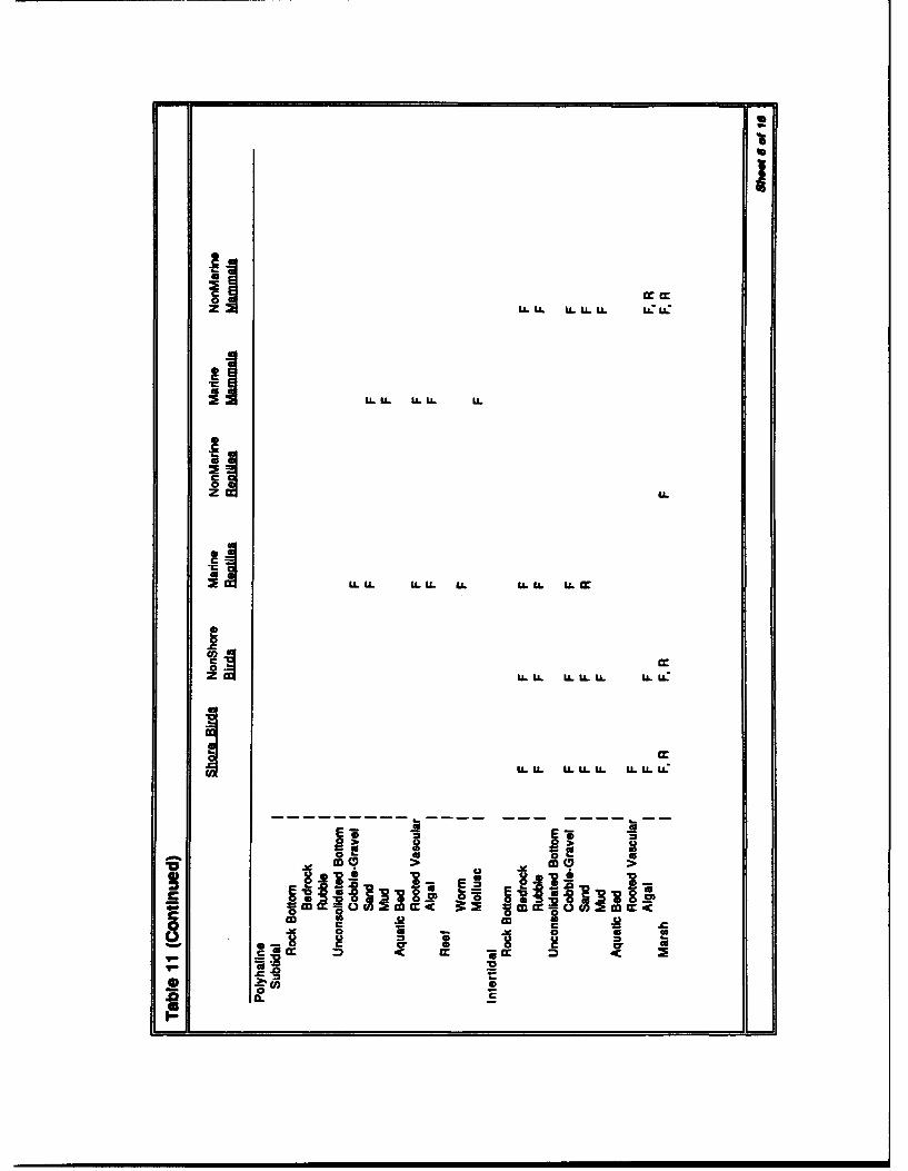
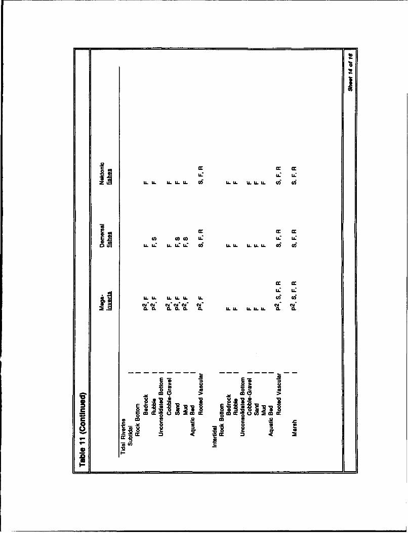
A matrix of all coastal habitats and their attributes is presented inTable 11. It was constructed by listing the CHCS (Table 8), the major bioticcomponents for each habitat type (Table 1), and assigning the appropriatefunctional attributes (Table 10). The total matrix does not have to be con-structed for each system; a smaller matrix including only the relevant habitatswill be needed. A matrix for the "Anywhere Bay" system is presented inTable 12. At first glance, even this matrix appears to be a "laundry list" of

11Chaplsr 2 Fraewr for a Coasal Hmbitt Evaludlon Method

ecological variables. Since it is doubtful that even a modestly sized systemmatrix could be filled in completely, the matrix is intended to serve as focusfor determining what is already known about a system and for deciding whatinformation is critical to evaluating the system. The critical attributes are thenselected and listed as a separate matrix. This critical attribute matrix is thebasis for all subsequent discussions and calculations. The choice of criticalattributes is obviously the most important step of the framework. Just as theselection of target species in a species-based method (e.g., HEP) injects aninherent bias to the analysis, the choice of critical attributes drives the interpre-tation of results from the framework. The choice of attributes must be madepurely on the basis of what is believed to be important to maintenance of thehabitat and its contribution to the functioning of the system. These choicesmust be made even if a "laundry list" is the ultimate result. Developing suchlists may not seem practical, yet, neither is a "minimal list" approach if it igno-res important data or ecological relationships. The extent of the critical attrib-ute matrix, however, need not be overwhelming. The example critical attributematrix (Table 13) details the structure and function of 10 different habitattypes. Less than a third of the original system habitat-attributes needed to beconsidered, and all of the attributes listed are commonly found in extantdatabases.

Step 5. Regional Attribute Values

After the selection of critical attributes, the next step is to assemble infor-mation on expected attribute values. Expected values are those data represen-tative of the same attribute, habitat type, and geographical region. For presentpurposes, geographical regions are classified by biogeographic provinces(Ekman 1953). These provinces are defined primarily on zoological distribu-tions, current patterns, and hydrological conditions and reflect broad-scalepatterns of species and community distributions (Table 14). Ekman (1953) isthe basis for virtually all subsequent schemes (e.g., Bailey 1976, 1978) andwill be used here. Phytogeographical distributions have also been described,but generally correspond to the same distribution patterns as the zoogeographi-cal provinces (Round 1981).

Information on attribute values can be found in many of the same docu-ments that provided data on habitat structure and functions, i.e., EcologicalCharacterization, Biological Report and Community Profile Series of theU.S. Fish and Wildlife Service, Species Profiles Series of the U.S. Fish andWildlife Service and U.S. Army Corps of Engineers, and NOAA's EstuarineLiving Marine Resources Program. Additional information can be found in thetechnical literature and governmental reports.

Regionally adjusted attribute values for the example system are presentedin Table 15. Note that polyhaline mud flats are broken down into two parts:A and B. In this case, Mud Flat B only supports 50 percent of the infaunanormally associated with that type of habitat. This condition in turn results in

12 Chaptr 2 Framework for a Coastal Habiat Evaluation MAtbod

reduced feeding opportunities for shrimps, crabs, fish, and birds. The ability todivide individual habitat categories into separate patches illustrates the flexi-bility of the framework. The patches can be analyzed individually and theresults easily incorporated into the framework. The degree of detail that aparticular analysis utilizes is left up to the end user.

Step 6. Habitat Mapping

Mapping of habitats and measurement of habitat areas (Step 6) followsassembly of the attribute information. The most cost-effective approach tohabitat mapping is to use pre-existing maps or data. Many agencies maintainmaps of economically important habitats such as oyster beds or seagrass beds(e.g., NOAA 1989). As previously mentioned, coastal wetlands are currentlybeing mapped by NOAA. Some state agencies have also produced habitatmaps of their coastlines. For instance, the Maine Geological Survey hasmapped all intertidal habitats (Timson 1977), and Texas has produced habitatmaps for both intertidal and subtidal habitats (e.g., Brown et al. 1976; White etal. 1983). As previously discussed, the distribution of many habitats can bededuced from sediment and salinity. This is particularly true of unvegetatedsediment habitats that are defined by these factors (e.g., polyhaline sand). Itwas assumed for the example system habitat map (Figure 2) that all unvegeta-ted substrate habitats could be mapped in this fashion. Marsh, rocky intertidal,and seagrass habitats were assumed to have been mapped by aerial photogra-phy and site visits.

While locating pre-existing maps is obviously a preferred course of action,it is essential that they not be used in an indiscriminate manner. Before anymap is used, the underlying information must be closely scrutinized to deter-mine its age, method of collection, and quality. A map will only be as goodas the data on which it is based. Another common source of error in pre-existing maps is scale. Maps of subtidal resources are generally produced byassuming the conditions at a sample site are representative of a particular phys-ical area or cell. A precise formula or even a general means does not exist todetermine the relationship between sample size and number, cell size andnumber, and the size of the system. Obviously, the more samples that aretaken in a cell and the more cells that are sampled, the more likely it is thatthe data will be representative.

When insufficient data are available to formulate an accurate habitat map,obtaining the information in a cost-effective manner is still possible. Aerialphotography provides a rapid, accurate, and repeatable mechanism for mappingmarshes and intertidal zones. Ground-truthing is required to ensure the accu-racy of the method, but can be done quickly and at low cost. Land-basedphotography can also be employed. Subtidal resources can be mapped with aremotely operated vehicle (ROV) or sediment-profiling camera. ROVs havebeen used to survey both species-specific habitats such as scallop beds (Lang-ton and Robinson 1990; Thouzeau, Robert, and Ugarte 1991) and generalfaunal assemblages. Sediment-profiling cameras have been used to rapidly

13Chapter 2 Framework for a Coastal Habitat Evaluation Method

map sediment distributions over large areas (Rhoads and Germano 1982).Diver-operated cameras may be effective in many situations. Maps can also beconstructed from the results of traditionally based sampling efforts such asbenthic surveys (e.g., Brown et al. 1976; White et al. 1983).

Once pre-existing habitat maps and other information have been obtained,the question of the best way to store, analyze, and present the data stillremains. The simplest method is to plot all of the habitats on a single map(e.g., Figure 2) and then use a planimeter to measure the area of each habitattype. Data from these measurements can be stored and analyzed on any com-puter spreadsheet program. A more expensive but more accurate methodwould be to use an image-analysis system. An image-analysis system mayconsist of a standard personal computer outfitted with an image capture card,image-analysis software, and a video camera. Maps are scanned into the sys-tem and the imaging software used to edit and measure the captured images.Most software packages also provide statistical analysis. Data can be stored onstandard floppy disks or mass storage devices (e.g., Bernoulli disks, replace-able hard drives, and optical storage) if a large volume of data is involved.Perhaps the most powerful method available is the Geographical InformationSystem (GIS). Davis and Schultz (1990) provided an overview of GIS struc-ture, operations, and practical considerations associated with its use. A moredetailed account can be found in Burrough (1986). As a rule, a GIS will betoo expensive to set up solely to perform the analysis outlined in this report.If, however, one is available and part of the required data has already beenentered, then the GIS may be the preferred option for data storage, analysis,and presentation.

Step 7. Attribute Measures

Step 7 is to provide a quantitative measure for each of the critical attri-butes. Data sources specific to the system under study have obvious priorityin the process. However, there will probably be little or no information avail-able on many habitat types within a specific system or for many of the attri-butes. In this situation, representative data from other systems in the sameregion may be substituted as long as the environmental conditions are repre-sentative. That is, data for a seagrass bed exposed to moderate wave actionshould be derived from seagrass beds in nearby systems in similar conditions.In some cases, compar ! le data may not exist, and attributes must be measureddirectly. Simenstad ei _. (1991) provided comprehensive recommendations formeasuring attributes of a wide variety of coastal habitats. Additional recom-mendations can be found in Price, Irvine, and Franham (1980), Nielsen andJohnson (1983), Baker and Wolff (1987), and Fredette et al. (1990).

14 Chapter 2 Framework for a Coastal Habitat Evaluatin Method

productivity by benthic invertebrate fauna were not significant, and amounts ofseagrass attributes in the system were increased (Table 17). Obviously, theoligohaline marsh was a limited resource to this system, and much of its con-tribution was lost. Planted seagrasses initially provide only a portion of whatis expected from natural habitats, but over time reach normal levels (Tables 17and 18). Further repercussions can also be estimated for other habitats and fordifferent time periods. In the example system, physical alterations associatedwith construction are predicted to result in changes in water flow and waterretention. Fresh water flows further into the estuary than previously, and amajor portion of mesohaline subtidal muds become oligohaline muds(Table 17). Over time, the oligohaline muds are predicted to become eutrophicwith suplus production of infauna (Table 18). Whether these losses and gainsrepresent an important long-term alteration of the system can probably bedetermined only with experience.

At the present time, predictive models or conceptual rules do not exist fordetermining what a specific change in an attribute or loss in the total amountof a habitat may mean to a system. The actual effect of trading habitats ortheir attributes will vary with the environmental status of each system. Forinstance, planting a seagrass bed in a highly polluted system may have a highprobability of failure because of water quality. Planting of marsh habitatwould be more likely to succeed because of the greater resilience of thesehabitats and could help improve water quality by sequestering pollutants.Planting either habitat in an identical but pristine system would probably havelittle discernible effect.

Another use of the framework would be to assess the current environmen-tal status of a system by comparing the current situation with estimated histor-ical conditions. In this case, measures of historical habitat areas or functionalattributes will probably not be available, so estimates must be made. Habitatareas can be estimated from existing distributions and historical records. His-torical attribute values can be assumed to be 100 percent of expected levels.This is a conservative approach since it presumes that a habitat will maintainnormal levels of function in the absence of human-induced disturbance. Asimilar assumption can also be made for modem habitats if there is sufficientreason to assume they are not affected by human-induced disturbance. Resultscan then be compared to determine the nature and extent of habitat changes inthe system. This comparison could then act as the baseline for determiningwhat attributes are the most important to restore or enhance.

16 Chapter 2 Framework for a Coastal Habitat Evaluakon MW•od

3 Discussion

This report describes a conceptual framework for a new method to assessenvironmental impacts from trade-offs of coastal habitats. It represents aninherently different approach to methods in current use in that it provides amechanism to examine system-wide repercussions of changes in the arealextent of habitats and their associated habitat attributes (ecological functions).It is essentially an inventory and accounting procedure based on the biologicalstructure and functions of habitats. Each habitat attribute is considered sepa-rately and its quantitative contribution is expressed as a percentage of expectedvalues for that region. Output consists of a listing of the habitat types in thesystem, their proportions, and a measure of their total contribution to thesystem (attribute values multiplied by habitat area). Although models are notavailable to predict what the precise effect of a particular alteration of a systemmight mean, this framework can be considered the first step towards a moreinclusive conceptual modeL By listing changes in each attribute separately, themethod permits a more detailed analysis than is generally performed and pre-vents underestimation of the importance of any one attribute.

The method outlined in this report is also different from existing proceduresin that it requires a substantial amount of initial effort. While some of thiseffort will be expended in assembling and compiling the information necessaryfor subsequent calculations, the bulk will be expended in consensus-buildingand decision-making activities. Unlike the conventional project-specificapproach, the new method is oriented towards establishing long-term environ-mental goals for the management of a system. The most important step in theprocess of constructing the framework, the determination of the critical attri-butes, requires that a consensus be reached concerning which attributes aremost important to the long-term health of the system. Likewise, the finalresults can only be applied if there is some common ground among managersregarding the direction in which the system should be managed. These deci-sions are presently made or negotiated every time there is a new projectImplementation of the new framework can act as a stimulus to formulating asingle long-term strategy for managing habitat trade-off issues. The expendi-ture of time and effort at the outset should be repaid by the elimination ofunnecessary and repetitive efforts associated with later projects. Even if com-mon ground cannot be established among decision-makers, the new frameworkcan provide a uniform approach for subsequent analysis and discussion of theissues associated with trading habitats.

17Chapter 3 Discussion

At the present time, case studies testing the framework am just gettingunderway. Examination of the framework's underlying assumptions and evalu-ation of its practical limitations am required before the framework can beapplied as a practical field method. The results of the case studies will bepublished as completed and further modifications and refinements of theframework made as experience dictates.

18 Chaptr 3 Dacssion

References

Adamus, P. R., and StockweUl. (1983). "A method for wetland functionalassessment. Volume 1. Critical review and evaluation concepts,"FHWA-IP-82-23.

Adamus, P. R., Clairain, E. J., Smith, R. D., and Young, R. E. (1987). "Wet-land evaluation technique (WET). Volume II: Methodology," OperationalDraft Technical Report, U.S. Army Engineer Waterways Experiment Station,Vicksburg, MS.

Armstrong, R. E. (1987). "The ecology of open-bay bottoms of Texas: Acommunity profile," U.S. Fish Wildl. Serv. Biol. Rep. 85 (7.12).

Bahr, L. N., and Lanier, W. P. (1981). "The ecology of intertidal oyster reefsof the South Atlantic coast: A community profile," U.S. Fish Wildl. Sery.FWS/OBS-81/15.

Bailey, R. G. (1976). "Ecoregions of the United States," U.S. Forest Service,Ogden, UT. (Map only; scales 1:7,500,000.)

_ (1978). "Ecoregions of the United States," U.S. Forest Service,Intermountain Region, Ogden, UT.

Baker, J. M., and Wolff, W. J. (1987). Biological surveys of estuaries andcoasts. Estuarine and Brackish-Water Sciences Association Handbook. Cam-bridge University Press, Cambridge, UK.

Bowen, M., and Small, M. (1992). "Identification and evaluation of coastalhabitat evaluation methodologies," Technical Report EL-92-21, Prepared byNormadeau Associates for U.S. Army Engineer Waterways Experiment Station,Vicksburg, MS.

Brown, L. F., Brewton, J. L., McGowen, J. H., Evans, T. J., Fisher, W. L., andGroat, C. G. (1976). "Environmental geologic atlas of the Texas coastalzone," Bureau of Economic Geology, The University of Texas at Austin,Austin, TX.

19Reference

Burrell, V. G. (1986). "Species profiles: Life histories and environmentalrequirements of coastal fishes and invertebrates (South Atlantic)--Americanoyster," U.S. Fish Wildl. Sery. FWS/OBS-82/11.57. U.S. Army Corps ofEngineers, TR EL-82-4.

Burrough, P. A. (1986). Principles of Geographical Information Systems forland resources assessment, Monographs on Soil and Resources Survey No. 12.Clarendon Press, Oxford University, Oxford, UK.

Couch, D., and Hassler, T. J. (1989). "Species profiles: Life histories andenvironmental requirements of coastal fishes and invertebrates (PacificNorthwest)--Olympia oyster," U.S. Fish Wild]. Serv. FWS/OBS-82/l 1.124.U.S. Army Corps of Engineers, TR EL-82-4.

Cowardin, L. M., Carter, V., Golet, F. C., and LaRoe, E. T. (1979). "Classi-fication of wetlands and deepwater habitats of the United States," U.S. Fishand Wildlife Service, FWS/OBS-79/31.

Davis, B. E., and Schultz, K. L. (1990). "Geographic information systems: Aprimer," Contract Report ITL-90-1, Prepared for Information TechnologyLaboratory, U.S. Army Engineer Waterways Experiment Station, Vicksburg,MS.

Dethier, M. N. (1990). "A marine and estuarine habitat classification forWashington State," Washington Natural Heritage Program, Dept. NaturalResources, Olympia, WA.

• (1992). "Classifying marine and estuarine natural communities:An alternative approach to the Cowardin system," Natural Areas J. 12, 90-100.

Diaz, R. J. (1982). "Examination of tidal flats: Volume 3. Evaluation meth-odology," U.S. Dept. Transportation Report, FHWA/RD-80/183.

Downing, J. A. (1991). "Comparing apples with oranges: Methods of inter-ecosystem comparison." Comparative analyses of ecosystems. Patterns,mechanisms, and theories. J. Cole, G. Lovett, and S. Findlay, ed., Springer-Verlag, New York.

Ekman, S. (1953). Zoogeography of the sea. Sidgwick and Jackson, Ltd.,London, UK.

Fay, C. W., Neves, R. J., and Pardue, G. B. (1983). "Species profiles: Lifehistories and environmental requirements of coastal fishes and invertebrates(Mid-Atlantic)--bay scallop," U.S. Fish. Wildl. Serv. Biol. Rep. 82 (11.12).U.S. Army Corps of Engineers, TR EL-82-4.

Fefer, S. I., and Schettig, P. A. (1980). "An ecological characterization ofcoastal Maine (north and east of Cape Elizabeth)," U.S. Fish Wildl. Serv.,FWS/OBS-80/29, (Five Volumes).

20 %fame"

Foster, M. S., and Schiel, D. R. (1985). "The ecology of giant kelp forests inCalifornia: A community profile," U.S. Fish Wildl. Serv. Biol. Rep. 85(7.2).

Fredette, T. J., Nelson, D. A., Miller-Way, T., Adair, J. A., Sotler, V. A.,Clausner, J. E., Hands, E. B., and Anders, F. L. (1990). "Selected tools andtechniques for physical and biological monitoring of aquatic dredged materialdisposal sites," Technical Report D-90-1 1, U.S. Army Engineer WaterwaysExperiment Station, Vicksburg, MS.

Hall, R. W., Dortch, M. S., and Bird, S. L. (1988). "Summary of Corps ofEngineers capabilities for modeling water quality of estuaries and coastalembayments," Miscellaneous Paper EL-88-13, U.S. Army Engineer WaterwaysExperiment Station, Vicksburg, MS.

Jaap, W. C. (1984). "The ecology of South Florida coral reefs: A commun-ity profile," U.S. Fish Wildl. Serv. FWS/OBS-82/08, Minerals ManagementService. MMS 84-0038.

Kantrud, H. A. (1991). "Wigeongrass (Ruppia maritima L.): A literaturereview," U.S. Fish Wildl. Serv., U.S. Fish Wildl. Res. ltI

Langton, R. W., and Robinson, W. E. (1990). "Faunal associations on scallopgrounds in the western Gulf of Maine," J. Exp. Mar. Biol. Ecol. 144, 157-171.

LaSalle, M., and Ray, G. L. (1992). "Assessment of habitat/resource evalua-tion methods for use in comparing estuarine and coastal habitats," Miscella-neous Paper EL-92-5, U.S. Army Engineer Waterways Experiment Station,Vicksburg, MS.

Lautzenheiser, R. E. (1972). "Climate of Maine." Climatology of the UnitedStates. U.S. Department of Commerce, Ashville, NC.

Lunz, J. D., and Kendall, D. R. (1982). "Benthic resources assessment tech-nique, a method for quantifying the effects of benthic community changes onfish resources." Oceans'82 Confrrence Proceedings: 1021-1027.

McLachlan, A. and Erasmus, T., ed. (1983). "Sandy beaches as ecosystems,"Developments in Hydrobiology 19. Junk, The Hague.

MEC Analytical Systems, Inc. (1988). "Biological baseline and an ecologicalevaluation of existing habitats in Los Angeles Harbor and adjacent waters,"Report to the Port of Los Angeles, September 1988.

Mullen, D. M., and Moring, J. R. (1986). "Species profiles: Life historiesand environmental requirements of coastal fishes and invertebrates (NorthAflantic)-sea scallop," U.S. Fish. Wildl. Serv. Biol. Rep. 82 (11.67).U.S. Army Corps of Engineers, TR EL-82-4.

21Peeeances

National Oceanographic and Atmospheric Administration. (1985). StrategicAssessment Branch. National Estuarine Inventory: Data Atlas, Volume 1:Physical and Hydrologic Characteristics. NOAA, Washington, DC.

_ (1989). Padilla Bay, Washington-Vegetative Communities(1989). Map. Padilla Bay National Research Reserve, Mount Vernon, WA.

_ (1991). Fisheries of the United States, 1991. National MarineFisheries Service, Fisheries Statistics Division. Silver Spring, MD.

Nelson, D. A. (1987). "Use of habitat evaluation procedures in estuarine andcoastal marine habitats," Miscellaneous Paper EL-87-7, U.S. Army EngineerWaterways Experiment Station, Vicksburg, MS.

Nelson, D. M., Monaco, M. E., Irlandi, E. A., Settle, L. R., and Coston-Clements, L. (1991). "Distribution and abundance of fishes and invertebratesin southeast estuaries," ELMR Report No. 9, NOAA/NOS Strategic Environ-mental Assessments Division, Rockville, MD.

Newell, R. 1. E. (1989). "Species profiles: Life histories and environmentalrequirements of coastal fishes and invertebrates (North and Mid-Atlantic)-bluemussel," U.S. Fish. Wildi. Serv. Biol. Rep. 82(11.102). U.S. Army Corps ofEngineers, TR EL-82-4.

Nielsen, L. A., and Johnson, D. L. (1983). "Fisheries techniques." The Amer-ican Fisheries Society. Southern Printing Co., Blacksburg, VA.

Odum, H. T., and Copeland, B. J. (1974). "A functional classification of thecoastal systems of the United States." Coastal ecological systems of theUnited States. H. T. Odum, B. J. Copeland, and E. A. McMahan, ed., TheConservation Foundation, Washington, DC.

Odum, W. E., Mclvor, C. C., and Smith, T. J. (1982). "The ecology of themangroves of South Florida: A community profile," U.S. Fish WildL Serv.FWS/OBS-81f24.

Pauley, G. B., Van Der Ray, B., and Troutt, D. (1988). "Species profiles:Life histories and environmental requirements of coastal fishes and inverte-brates (Pacific Northwest)-Pacific oyster," U.S. Fish Wildl. Serv. FWS/OBS-82/11.85. U.S. Army Corps of Engineers, TR EL-82-4.

Peterson, C. H., and Peterson, N. M. (1979). "The ecology of intertidal flatsof North Carolina: A community profile," U.S. Fish Wildl. Serv.FWS/OBS-79/39.

Phillips, R. C. (1984). '"he ecology of eelgrass meadows in the PacificNorthwest: A community profile," U.S. Fish Wildl. Serv. FWS/OBS-84/24.

22 Remre,

Porter, J. W. (1987). "Species profiles: Life histories and environmentalrequirements of coastal fishes and invertebrates (South Florida)--reef-buildingcorals," U.S. Fish Wildl. Serv. FWS/OBS-82/1 1.73. U.S. Army Corps ofEngineers, TR EL-82-4.

Price, J. H., Irvine, D. E. G., and Franham, W. F. (1980). The shore environ-ment. Volume I: Methods. The Systematics Association Special Volume No.17(a), Academic Press, New York.

Ray, G. C. (1975). "A preliminary classification of coastal and marine envi-ronments," IUCN Occasional Paper No. 14, International Union for Conserva-tion of Nature and Natural Resources, Morges, Switzerland.

Rhoads, D. C., and Germano, J. D. (1982). "Characterization of organism-sediment relations using Sediment Profile Imaging: An efficient method ofremote ecological monitoring of the sea-floor," Mar. Ecol. Prog. Ser. 8,115-128.

Round, F. E. (1981). "Dispersal, continuity and phytogeography." The Ecol-ogy of Algae. Cambridge University Press, UK.

Seller, M. A., and Stanley, J. G. (1984). "Species profiles: Life histories andenvironmental requirements of coastal fishes and invertebrates (NorthAtlantic)--American oyster," U.S. Fish Wildl. Serv. FWS/OBS-82/l 1.23.U.S. Army Corps of Engineers, TR EL-82-4.

Shaw, W. N., Hassler, T. J., and Moran, D. P. (1988). "Species profiles: Lifehistories and environmental requirements of coastal fishes and invertebrates(Pacific Southwest)--Califomia sea mussel and bay mussel," U.S. Fish. Wildl.Serv. Biol. Rep. 82 (11.84). U.S. Army Corps of Engineers, TR EL-82-4.

Simenstad, C. A., Tanner, C. D., Thorn, R. M., and Conquest, L. L. (1991)."Estuarine habitat assessment protocol," Puget Sound Estuary Program, Pre-pared for U.S. Environmental Protection Agency, Region 10, Office of PugetSound, Seattle, WA.

Stanley, J. G., and Seller, M. A. (1986a). "Species profiles: Life historiesand environmental requirements of coastal fishes and invertebrates (Gulf ofMexico)--American oyster," U.S. Fish Wildl. Serv. FWS/OBS-82/1 1.64.U.S. Army Corps of Engineers, TR EL-82-4.

_ (1986b). "Species profiles: Life histories and environmentalrequirements of coastal fishes and invertebrates (Mid-Atlantic)--Americanoyster," U.S. Fish Wildl. Serv. FWS/OBS-82/l 1.65. U.S. Army Corps ofEngineers, TR EL-82-4.

Stout, J. P. (1984). "The ecology of irregularly flooded salt marshes of theeastern Gulf of Mexico: A community profile," U.S. Fish Wildl. Serv. Biol.Rep. 85 (7.1).

23Resfeenm

Teal, J. M. (1986). "The ecology of regularly flooded salt marshes of NewEngland: A community profile," U.S. Fish Wildl. Serv. Biol. Rep. 85 (7.4).

Thayer, G. W., and Fonseca, M. S. (1984). "The ecology of eelgrass mead-ows of the Atlantic Coast: A community profile," U.S. Fish Wildl. Serv.FWS/OBS-84/02.

Thouzeau, G., Robert, G., and Ugarte, R. (1991). "Faunal assemblages ofbenthic macroinvertebrates inhabiting sea scallop grounds from easternGeorges Bank, in relation to environmental factors," Mar. Ecol. Prog. Ser. 74,61-82.

Timson, B. S. (1977). "Coastal Maine geologic maps," Maine GeologicalSurvey.Open File Report 77-1, 113 maps at 1:24,000 scale, Augusta, ME.

United States Fish and Wildlife Service. (1980). "Habitat evaluation proce-dures, ESM 102," Division of Ecological Services, Washington, DC.

White, W. A., Calnan, T. R., Moerton, R. A., Kimble, R. S., Littleton, T. G.,McGowen, J. H., Nance, H. S., and Fisher, W. L. (1983). "Submerged landsof Texas," Bureau of Economic Geology, The University of Texas at Austin,Austin. TX.

Whitlach, R. B. (1982). "The ecology of New England tidal flats: A commu-nity profile," U.S. Fish Wildl. Serv. FWS/OBS-81/01.

Wiedemann. A. M. (1984). "The ecology of Pacific Northwest coastal sanddunes: A community profile," U.S. Fish Wildl. Serv. FWS/OBS-84/04.

Wiegart, R. G.. and Freeman, B. J. (1990). "Tidal salt marshes of the South-eastern Atlantic Coast: A community profile," U.S. Fish Wfldl. Serv. Biol.Rep. 85 (7.29).

Zale, A., and Merrifield, S. G. (1989). "Species profiles: Life histories andenvironmental requirements of coastal fishes and invertebrates (SouthFlorida)--reef-building tube worm," U.S. Fish Wildl. Serv. FWS/OBS-82/11.115. U.S. Army Corps of Engineers, TR EL-82-4.

Zedler, J. B. (1984). "The ecology of Southern California coastal saltmarshes: A community profile," U.S. Fish WildL Serv. FWS/OBS-81/54.

Zieman, J. C. (1985). "The ecology of the seagrasses of South Florida: Acommunity profile," U.S. Fish Wildl. Serv. FWS/OBS-82/25.

24 Referenoes

Uln Habitats

Maximum Extent ofEstumrine Influence

Figure 1. Boundaries of Anywhere Bay System

Uwah

Sand *d A 3l~dImt

Figure 2. Habitat map of system before project

NMw Dovdopmd

F Mure * 3. Hbttm apo yse ferpj

Table 1Structural Elements of Biological Communities

Elemuis Examples

Microllora Bacteria, Fungi

Microalgae Diatoms

Maoaigae Uiva, Kelp

Vascular Plants Seagrasses, Marsh Grasses

Meiofauna

Meioinfauna Nematodes

Meioepifauna Copepods

Macrotauna

Macroinfauna Polychaetes, Clams

Mobile Macro-Epitauna Amphipods. Isopods

Attached Macro-Epifauna Barnacles

Megainvertebrates Lobsters, Crabs, Shrimp

Demersal Fishes Flounder

Nektonic Fishes Anchovies

Shorebirds Willets, Tems

Non-Shorebirds

Marine Reptiles Sea Turtles

Non-Marine Reptiles Rattlesnakes

Marine Mammals Seals, Otters

Non-Marine Mammals Raccoons

Table 2

Evaluating Coastal Habltats-Steps In the Process

I. Identiy system boundaries.

2. Collect and compile backgound information.

3. Identify habitats.

4. Identify critical structural and functional attributes.

5. Summarize expected range of habitat attibute values.

6. Map local habitats.

7. Estimate or measure the functional attributes of habitats.

8. Express functional attributes (Stop 7) as a percentage of regional average (Step 5).

9. Multiply habitat area by regionally adjusted atrbute values (Stop 8).

10. Compare values for habitat diversity (number of habitats) and total attributes (Slep 9) for the entire systmnover time or between different management scenarios.

Table 3Habitat Types and Total Areas (hectares) for Anywhere Bay

[Hatia Type sew Prejeet Af Project= == =-

Marine Sand 2.000 2,000

Marine Rocky Intertidal 60 60

Polyhaline Marsh 800 80o

Polyhaline Grass 250 250

Polyhaline Constructed Grass - 100

Polyhaline Sand 2,500 2,400

Polyhaline Intertklal Mud Flat 100 100Mud Fat A 50 50Mud FlatB 50 50

Mesohaline Subtidal Mud 100 30

Mesohaline Marsh 400 350

Oligohaline Marsh 800 0

Oligohaline Subtidal Mud 0 50

Lost to Development 860

Total 7,110 6,250

Table 4

Background Data Sources

Dole Type Date Seem

System Boundoie NOA Estuwine Inventory AdesUSGS Hydrological Unit MapsUSGS Topographic Maps

Topography USGS Topographic MapsNOM Navigation Charts

Geology U.S. Geologica Survey

State Gwe ical Survey

Meterology U.S. National Weather Service

Hydrology U.S. Geoogica SurveyHydraulic Models

Sediments U.S. Army Corps EngineersSol Survey

ChemisyWManr Quality U.S. Envionmenisl Protection Agency,State Water ResourcesWater Oualily Models

Table5Habitat Classification Scheme of Ray (1975)Coastal Envhemwnts Cowl-Aaeeutd Environments,

Exposed Submarme vegetabon bedsRlockty substrate mgee

Cal1cereous Vascular plantsWeeldy calcamous or nonoeicarsous Estuaries

Unoonmoklidmtd substrate tdxoeuhalineLow organic content PolyhalMin

Gravel MesohalineSand OligohalineSil L~agoonsClay Hypersalke

High organic consent Euhalinprotected Mixoeuhaline

Rockty substrate Po alyhaneCcareous MesohalineWesidy calcareus or noncalcareous Oligohale

Unconsokldaed substrat Tida salt marshesLow organic content Nontdal salt marshes and flats

Gravel MaNgrveSand Drainage basinssolt Extentclay Type

High organic conwtenDelta

Ke* beds SpoilCoral reek near oontinente Rleefs

Covmf erbad ___Cmlrotrw*r&Specal leIrest

Drownedl reestmtuterleesInsular envromenwtsfam fW okreContinental shelves Sesaon~al fish concentrations

Offslope enronnients lnswre circulation cob

Larger scale circulation cellsUpelhing systemns

Table 6The Habitat Classification Scheme of Cowardin et al. (1979)Y

hMarn Sbtkda Rock bottomUnconsolidated bottomAquatic bedReef

Intertidal Rocky shoreUnconsolidated bottomAquatic bedReef

Estuarine' Subtidal Rock bottomUnconsolidaled bottomAquatic bedReef

Intartidal Rocky shoreUnconsolidated bottomAquatic bedPAWStreambedEmergent wetlandScrub4crub wetlandForested wetland

Rivenine Taid Rock bottomUnconsolidated bottomRocky shoreAquatic bed

I I Emergent wetland(Coastul habitats only.'Salinity modifiers include Hypersaine, Euhaline, Polyhaline. Mesohaline, Oligohalmne.

Table 7Habitat Classification Scheme of Dethler (1990)

Mari" Esuomne

Inlelidkw intelidalRock (Wid bedrock) Bedrock

Exposed OpenPartially exposed HardpanSemiprotecled and protected Mixed coarse

Boulders OpenExposed Partly endosedPartially exposed SandSerniprotecied and protected Open

Hardpan Partly enclosedCobble Mixed fine

Partially exposed Partly enclosedMixed coarse Lagoon

Semiprotected and protected Mixed fine and mudGravel Partly enclosed

Partially exposed LagoonSemiprotecied Channel-Slough

Sand MudExposed and partially exposed Partly enclosed and closedSemiprotected Organic

Mixed fine Partly enclosedSemriproteced and protected Backshore

Mud ArficialProtected Reef

Organic (wood chips, maine deritus)Artificial SubtidalReef Bedrock and boulders

OpenSubtidal Cobble

Bedrock and boulders OpenModerate to high energy Mixed coarse

Cobble OpenHigh energy Sand

Gravel OpenHigh energy Partly enclosed

Mixed fine Mixed fineHigh ewergy OpenModerate energy Sand and mudLow energy channel

Mud and mixed fine OrganicLow energy Artificial

Organic ReefArtificalReef

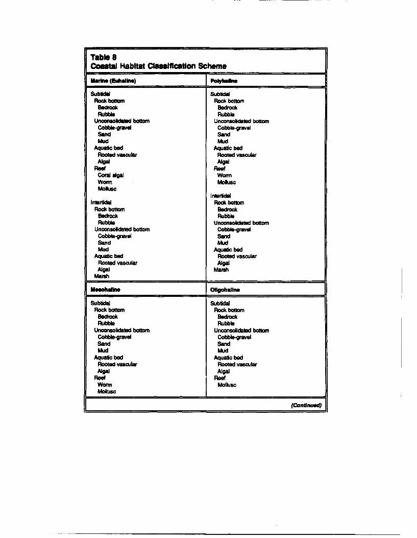
Table 8

Coastal Habitat Classification Scheme

Madm (Eur=am) -Subodal Sublidal

Rock beam Rock bottomBedrock BedrockRubble Rubble

U o d bottom Unconsolidated bottomCobble-gravel Cobble-gravelSand SandMud Mud

Aquatc bed Aqjauc bedRooted vascular Rooted vascular

Reef ReefCoral gal WormWorm MoluscMollusc

IntortdItrtrdal Rock bottom

Rock bottom BedrockBedrock RubbleRubble Unconsolidated bottom

Unconsolidated bottom Cobble-gravelCobble-gravel SandSand MudMud Aquatic bed

Aquatic bed Rooted vascularRooted vascular AlgalAlgal Marsh

Marsh

[Mesohulnm Olgohhlkn

Subtidat SubdklalRock botom Rock botlom

Bedrock BedrockRubble Rubble

Unconsolidaled bottom Unconsolidated bottomCobble-gravel Cobble-gravelSand SandMud Mud

Aquatic bed Aquaic bedRooted vascular Rooted vascularAlgal ANa

Roef ReefWorm MolluscMolusc

(CondnuO

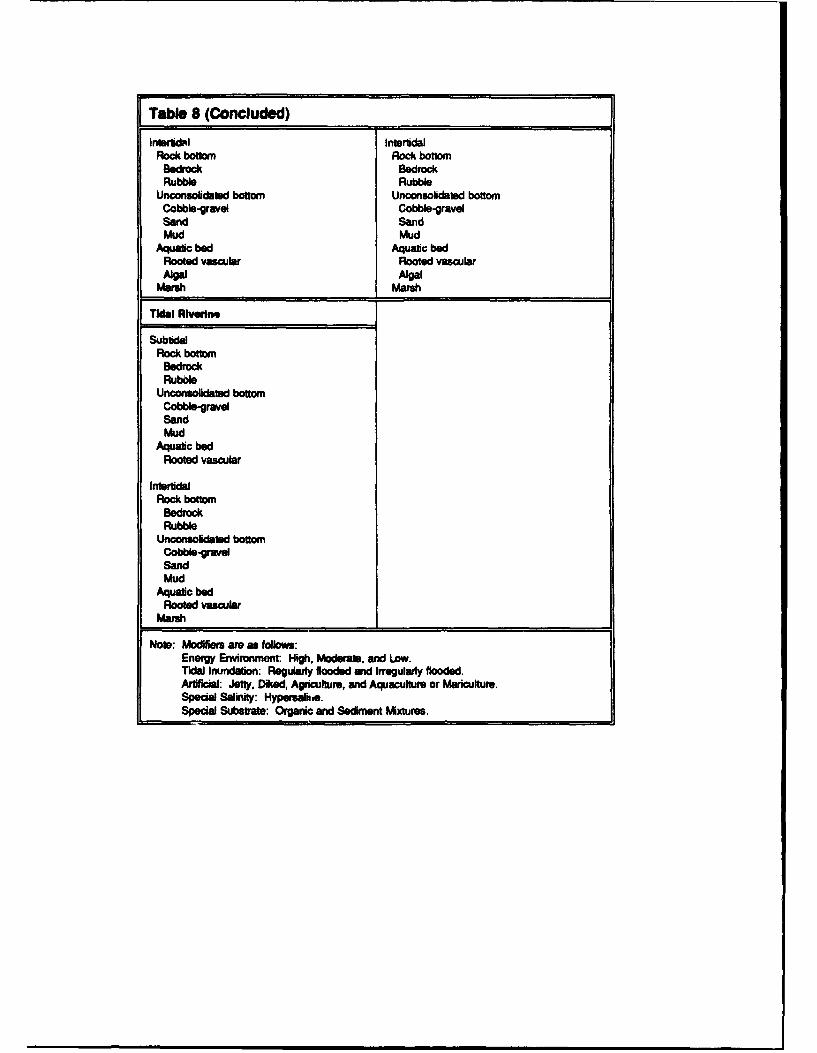
Table 8 (-Concluded)

lnatkstil ItiaRock bottom Rock bottom

Bedrock BedrockRubble Rubble

Unconsolidated bottom Unconsolidated bottomCobble-gravel Cobble-gravelSand SandMud Mud

Aquatic bed Aquatic bedRooted vascular Rooted vasculargA19 MA19

Marsh Marsh

ITWda Rivering

SubtidalRock bottom

BedrockRubble

Unconsolidated bottomCobble-gravelSandMud

Aquatic bedRooted vascular

InftertidRock bottom

BedrockRubble

Unconsolidated bottomCobbleaVelSandMud

Aquatic bedRooted vascular

Marsh

NOte: Modifiers are as follows:Energy Environment: High, Moderate, and Low.Tidal Inundation: Regularly flooded and Irregularly flooded.Artificial; Jetty, Diked, Agricufture, and Aquacufture or Mariculture.Special Salinity: Hypersalhe.Special Substrate: Organic and Sediment M.ixtures.

Table 9

Coastal Habitat Profiles

Oystr Rosh

Bahr, L N., and Lanier. W. P. (1961) - Georgia Intertidal ReefsBurell, V. G. (1986) - American Oyster-South Atlantic.Couch, D., and Hassler, T. J. (1989) - Olympia Oyster.Pauley, G. B.. Van Der Ray, B.. and Troutt. D. (1988) - Pacific Oyster.Sellr, M. A.. and Stanley, J. G. (1984) - American Oyster-North Atlantic.Stanley, J. G., and Seller. M. A. (1986a) - American Oyster-Gulf of Mexico.Stanley, J. G., and Seller, M. A. (1986b) - American Oyster-Mid-Atantic.

Othe Molluso Habitats

Bay ScallopFay, C. W., Neeves, R. J., and Pardue, G. B. (1983).

Sea ScalopMullen, D. M.. and Moring, J. R. (1966).

Blue MusselNewell. R. I. E. (1989).

California Sea Mussel and Bay MusselShaw, W. N., Hassler, T. J., and Moran, D. P. (1968).

Intertidal Flats (Need PacIfic Coast)

Peterson, C. H., and Peterson, N. M. (1979) - Nortlh Carolina.Whitlach, R. B. (1982) - New England.

Sandy Beeches

McLachlan, A., and Erasmus, T. (1983).

Dunes

Wiedemann, A. M. (1984).

[Corals

Jaap, W. C. (1984) - South Florida.

Porter, J. W. (1987) - South Florida.

Worm Reefs

Zale, A., and Merrileld, S. G. (1989).

Mangroves

Odum, W. E., Mdlvor, C. C., and Smith, T. J. (1982) - South Florida.

Marshaes

Stout, J. P. (1984) - Gulf of Mexico.Teal, J. M. (1986) - New England.Wiegart, R. G., and Freeman, B. J. (1990) - Southeastern Atlantic.Zedler, J. B. (1984) - California.

(Continuod)

Table 9 (Concluded)

Kantlrd, A. H. (1991) Ruppia.Phillps. FL C. (1964) - Pacific NorthwestThayer, G. W., and Fonseca, M. S. (1984) - Atantc Coast.Zieman, J. C. (1965) - South Florida

Foster, M. S.. and Schiel, D. R. (1965) - West Coast.

Unvegetatsd Unconsoldated (Soft-Bottom) Subtidal

Anmstrong, N. E. (1967) - Texas.

Rocky Inartidal

CensldMated (Hard Bottm) Subtldul

Table 10Functional Attribute Hierarchy of Simenstad at al. (1991)

ReproduoUon JRefug, and Physiology

General GeneralLight SalinitySalinity SoundSound TemperatureTemperature TurbidityTurbid•ty Water/sediment qualityWater/sediment quality Physical complexity

Elevation Bathymetric featuresInterfidal Horizontal edgesSubtidal Vertical reliefRiparian Water movement

Substale Biological complexitySediment MacronEmergent vascular plants Emergent vascular plantsMacmoalgae Submergent vascular plantsRiparian vegetation

GeneralCarronDetritusGraveingLightSalinitySoundTemperatureTurbidityWater/sediment quality

PlantsMicroalgaeMacroalgaeEmergent vascular plantsSubmergent vascular plants

InvertebratesBenthicEpibenthicNeustonicPelagic

VertebratsDemer"alWaer" columnNeustonicTerrestrial

00 cc c0 000 U. CO000c

0.0. 0. 0.0 04.0.m0cc, -, y - w. 0.0 0. al0.

U.Lh IL IIL IL 0L cQ. a.~u CLCL CLILILI

CIC LL CI CLL LL C6c C6 C 6 U L C6 C6CIL L0C. C 0.0 . IL.0ILI.0 . a. . a.0.a. 0.a.0a.

U.UI. ILCL I L C ILU. a. a.ILU

C'1C% Cii Cim cm C -4 CiiCi Ci i i

CLLU IU.&ma C.

IL I J cii Ci.& 0.I 0 L La

0.0LL L . 0. 0.0.0LL . 0.0.0

0.I0I.L LI 0 L L I 0.0a.0

--- I- -- I- L~

U) _) 0w 3IL9 I L . C. LCLI I u I L LC3 Go w co ww IO

*I -C .tCL I a-L LS L0. 0 .a

-----------ii_______________ U

04

m II

ii~L ULL IIL . U. U: I: LC

LL L L LL L L L C6 d C ccu aw~a C6i iCuu avd

a. a. a. CL CLL CL9L 0.00I LLC U LL 000a a

0. 3. 0.0.0 0.0 0.0.0. m.L u~ . 000

0 a.

0 -

32 3200 cc 0cc

ii L~L ILLU.. LCL

iiLL U. LLU.. LL LL .L L L

ILIA LL L L L LL L.

IL LLU. ILIL L U. ILL:

I o >' 8oO

CC .0 1-

00

I-I

U. L U L.IIUU.LL LLLI 003 W0 LL .uuL

IL L C C CVN D.¶ CLa~ n. c CL CL L a LC

LL L LL. LL ... L I LL U. I.L IUL

IL L C C IL I .a I LI

LL U. U. LLU. LL . U LIL LL ILL LLL

cu.0y. cm. 0m.0cy. C14 0.0. c.0J. 0C.0C.0. .

CL 0. 0

0.0. _I .0.I0 _L C . 0.0 I.0 CL IL0. 0.00

-i - - - -- -- - - - -

03. 1 .1 :201 . o

2.5

IIL

ULL U. UU. 00 LL C6C wC LL LL ULL.U. LL C 600

IImLL LLLL: LL:U

LLL LLLL L L U c6 6 6 c c

cm y m u-i, cci cm . . . cm1 cSI- cm-a0.0a. a... I.0 C0C.C L0. LU. LA . LL L . CL CL ..

>l -ici

in0 IEEcow 0Cc

cr. M c0

ID

I' LL LL. .L LL L

0

zIL. LU. U. LLL U.LL

IL ELL. LLILLLA. LL. U.LA

E 7a

=60 0 -0

coc

'D~ CCm c

CJr 11 SI3

U)00 U) 002 U 0(J ) ) (10 U. (D MYi~W (Vm N~(% (dV(Vm (0.0 0L . 0.0 0.0L L . a.. 0. C0.0.0.

(0 LL ( LL( LL. .U 0 0 0 L.U.L

cm, cmi &c1N W W cm CJ. -4 cy& cy-cc, ccvCJCdI.0 C .. 0 0.C C L0. C.0 0.0C.0. I 0.0.C0.I

U U. U. L L JL L. I L A.U . tLL. UcyJ~ cy cy C. C4 V(C C %I00.. 00. 0. IL ILI0C.0. IL.0.0.

LLU U. u6C C LuO U L . C6d0

C.,C'i, cm cy XX ~ ci* aa &a0.0.CL.0. a..a0.0 . a... a.a.0a.

U.

ILL L. U.UL. LL C LLU.LLh. LLLLU.

cmC-4~c CVi tV (V CVVC NC',

0. 0. a .a . 0. 0.

00 0... 00. a. 0. 0. 0.0a.0. 00

------ - -- - - --- ---

00

Sm I

00o

LL LL uLL L c 6 dLLc .L L LL c c c

ii w U)LU LL L A: LA: L:L:LiLLA: LL L: L: 6c uuc6 LLc LUu. U. Lu..u. o6 c6 6

LL LLL.L: &C U:a :Lj LL LL. L ~L U. U. LL 6 Uc.LLc c

cmuytcycm y cycm u c m .iul. c, . -u u-u-u oCY-C6

CL L LCL CLL CL . CL 00. LL LL . MI ( 0 .0

a xE5E

a 0 0

co w 0 W.x 00 x.2

cc CI C

I

c cr

LL. LLL LLU.U. U ILU:

ii

u..u. u utu.. u.LL

LLU. ILL L L UU-

EiE

co ~ ~ 40-c

0 10! 0 _,

cc cc m

cy cm Nj CYN N C1400 0.00. C . 0.0 0. C0.0.0.I C

UIJ

LLU LL UL-U. ULL. U. U.

2 -- UUU. L U-U-U. LLC 0 6L Ww C

a.N N 0. a. 0. C IL CNN ILCL CLIL

0.0 0..0 0.0 0.0.0L L L. 0.0.0.L

U-U U-CL U. I--U U.U.U- I C C

CL 0.C I L 0. 0.0 0.0... a.0a.0I

U-U. U. LL L L U-U.L L LLLL

0.0 0.0 -L 0.0L . 0.0.0. 0. 0. 0.

U.U.U U-U U- U--Ua-U

C 0C .0.0 . ILC I I 0.0 C. a.0.0. IL CL0.

E1 E

0.o

0 0 028c

0.0. ~0. 0.0 0.0.;c o 0.00 (D .0.

00

0 00

ID

LA:LL IA LL: LL:

zeL L L LL 6 C6 C6 LLI. LL UU.. L c6 c6 c6

0 ~~~~ 00. IL. I IL

LLu LL L L L L L 6 c6 dd u-- u.u.. W 6I

M LC .U. a. C-L C0 L . U LL. a

a

0cc

0c o C0 9 G

rZ-~u LLLLLLLL LI:LL:

0

z LL

ZOLLLU.. ILL LLJ U.U

1.. a -aE a

8 0-c spmc5 MMM 032=mc ) c

~0 0

a .0 i - V8 or0

UPO

IL L.I J. a. a. I.

U.U. L L L & . L. LA.LL CL LLLLLL C6l cd 4 LL L C6 CJ

CLI .CLC LL C L L .IL C

0 LLi. LL U) LL LU. LL U)Cvl NI cm, cy. &&- & cm, &y &

IL IL. C. 1.1I.1. U. CL

(am .0 0. 0.0.0 L . 0. 0. c

i. 0.C C . .C 0. 0.

I. C -IL ICL .a - I -C

0. 00.. 0C00 000 0. 0.L

C..0 CL C0. I0I.0.C C L 0. 0. 0.

oa co

cc 0

M~ CDarI-:Iitc

cc cc cc

LL L LL L LL C6 L LL LL U LL 6 C

0 LU. LA: U. L:LA 6 L.L L U..Uu LL C Cl

~~~~~I~~~L LL LUC) U.LIIUCLA:c

U L LL U.LL U.. C6 Cl)cy,*~ cm, Cy1 c c 4,y cy

0.L IL .0 I0MCL I . LL L .ILILU. IL 9.

E5

0 0

= * c c =2 aC coc .c c 0 wcCO co

0

CC m

ffrl Z

W.4

LL LL LL LLLL LA

21ILL

ILU.. >LIU >

I *j~~rii~ I djIe

OD

0

-0

C* C

0m e7

~ cc

wd& (0

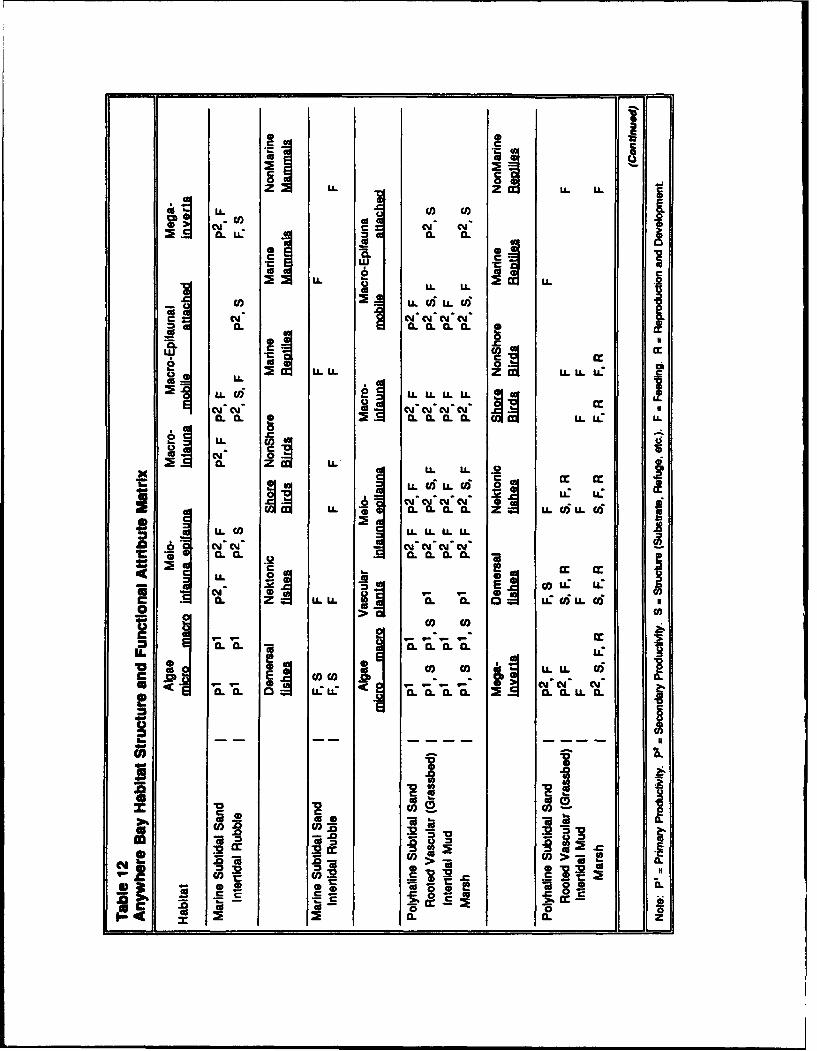
c~Cc

LL z OLL)zLL

I0.L ( a.w CLor

* LL LL

U. C.0.0L0.

SU. U. 0~ .LLz LA LLL:c

u. c6 LL L L

CV. I. II . cy . .L.C

LL

C0. L LL LL .S2

LL c6 LLU. C6U a

IL %SE L LdL

CQ -CMC.C.C- CM

LL CL a. LL c6 L c6

0.0. ~ .~ a~o uco

CL CLC L LI

CD

x CIO) w

20 250CD 0 a Cz

o Cc CLC L

CLUL Ljj c IL0

-cc

- -

0.0

z a:

om 60 y 00

*CL .EI@ CL Z

*l'c , 0c 00a.- 0.z r-

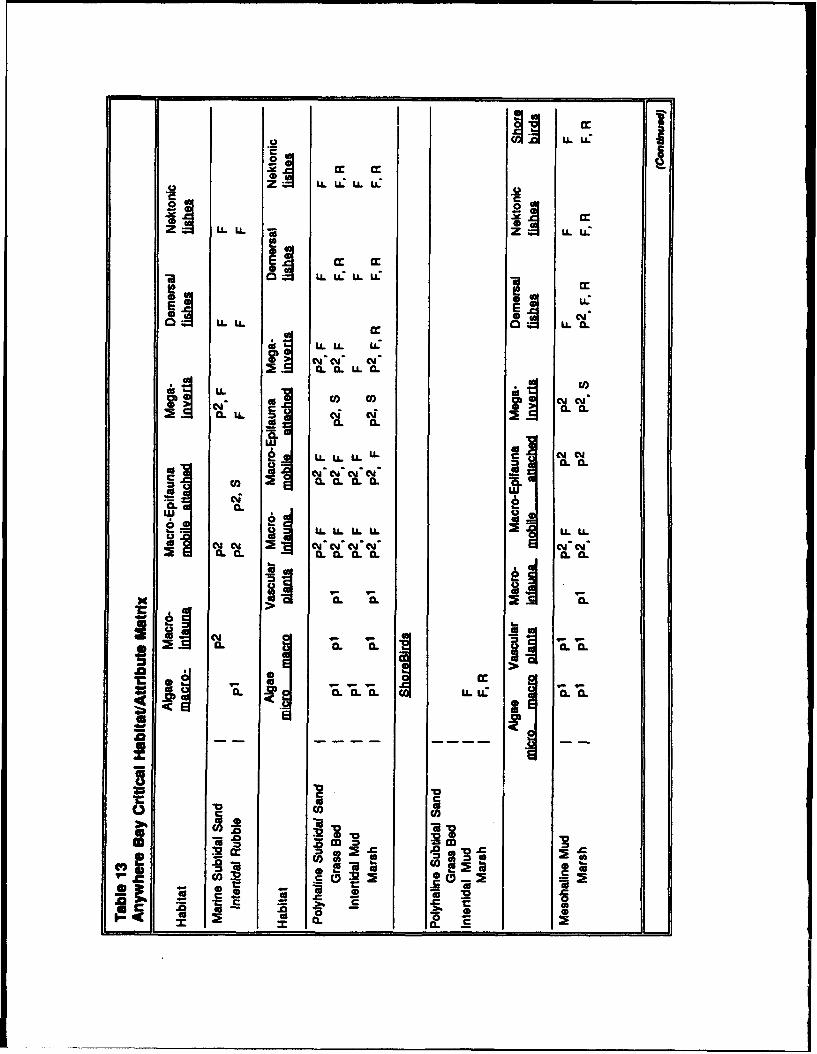
LLL Zi: U. L.

LL U.LLL LL

wi LC L L

~d U. U 1- LC

C'a..0

tiU.ILU. U. U c c

2 1 i£L U. 0.. 0.U.L

a.a.0a. LL U:.0

fla

U o -a

Ii LL

kIL

0.

U.LLjI

0CLzILcoS

C4 S- a

Co .i 00 0

Table 14Coastal Biogeographic Provinces of the United States1

Provinfe (Altemrnatve Temnolegy) ApproxnImat Geographc Boundaries

Arcecan Southern Greenland to Cape Cod.

Virginian Cape Cod to Cape Hatteras.

Carolinian Cape Hatteras to Cape Canaveral.

West Indian (Flodian) Cape Canaveral to Cedar Key, FL.

Louisianian Cedar Key, FL, to Port Aransass, TX.

Californian Cape Mendocino to Mexico.

Columbian (Oregonian) Cape Mendocino to Vancouver Island.

Fjords (Aleutian) Vancouver Island to Up of Aleutin Island Arc.

Pacific Arctic (Alaskan) Coast of Alaska not including Aleutian Island Arc.

Pacific Insular (Hawaiian) Hawaii

' After Ray (1975) and Bailey (1976, 1978).

o0c o M r o cD00m ece om eeoc 0 0

cc eCO 0 eCe(C ecoc 000 o rr- 0 00 000- - -- - -- - -- -

cc emf) 0 cooo000m 0000 Cc 0

000 0 0l 000 0 0 0o l 0 en

00 0 W)0 0 a 0 0 L

CC

c00 0

- - a- w C4 - - -. * m

I -a - - aL E E

.0 go C 30 M Z . 2c0- C t c LC 0 00 0 0.

j CL = jL trr0 ccm om In 0.

N ccrser e I

-Z 0 -c cc c c

ICI

0 0 00 00000000 0000 00 000

O CICO 00000000O 0000 00 0000 000 000 000 00) 0l Vq eVVC l Vl wm

00 0 00 0 0 0

0 I 0000j 00000000 0000 00 0

ca~0 00000000 000000

ISO c 0 0U) W) 0D Oln Go

0 ~ C~ in cc-c0 )0cr. 0 W Vfl 0 InN CO N

CL U. cc . .

0o 0 00 0 0c0L 0L 00= = m t 0 0c

0 - f mo 0d CLM QW- -t0 . Cw.020 t C= ZrL LL--

Ccm -c L> S. > co CIIC6 .N 0

.0 002~~u e o o

A WF F F0 0 W=

M > aozzI, co z z zz z

0000 00000000 0000 00 000

ca0 Y000 00000000 0000 00 0

00

ca 0 w000 00 00 0000 000 0

0 00 00 -r- 00 C l-a 01C.D . . . * * .0

0000 00000000 0o0In W) W) in U) W) mnaW ani n mnU n U n Vmn0 Y 011m 0 01 1 10 0 010M1 .m .M5 YC YCMCi C Y

0 0 00 0 0*0 0 00 0 0

it ccS~ 0 W)t 0 in. a * ~ C CDV W COV . a s S S

-L LLI L

.5a ca 4~00 . A~ 5c Ecd5

C .-a .a .caC I. aC1 .L .m

caI a C L a0 - v vm Sfl r_0.0. J, -10 c

060 e77 -. 0 6. C 224u is E Emc c c cS0 00I-.22 OZ O (a ~ S*~ zc, z zzzz

PAb.

0004 00 00 0 0 0 00 0

0 Y0~ 0 o0000000 00 00 0

X0_'5' CM W cm 0 )c 4ny

COO 0 0 00 0000000 0oc 00oCD - .Co0

CYC C Y mc CD CN J CY NC%1CY CY JN 04 .Y CM

0 0 00 0 0S0 0 00 0 a

0 qo 0000 0.O to to C.O .co CD (D CO M

0 0000 0 0

0 0 0000 0 a4t jj &14L _YC Cj

o CL C 00CL. (L E ;-~ jjj 5cI! ii ii"0 S

Form Approved

REPORT DOCUMENTATION PAGE OMB No.o 07

Public 0" 1g burden for this collection of information is estimated to average I hour oer reveonse. includi g the tim. for reviwin structaonl. searching eastig data sources.g .•and maintaining the data needed. and conalting and reiein the c.1ol o1 ,nformalion e coment regrding th1t burden estimatea .ora h ect of thiso of information. including suggestions for reducing this burden, to Washington ieadauarters Services. Directorte o formation O•erations and Reports. 12, 15 fferson-

Davislogihway, Suite 1204. ArlingtOn, VA 22202-4302. and to the Office of Management and Budget. Paperwork Reduction Project (070d-01NI) Washington. DC 20•0•3

1. AGENCY USE ONLY (Leave blank) 2. REPORT DATE 3. REPORT TYPE AND DATES COVEREDIFebruary 199:4I Final renort

4. TITLE AND SUBTITLE S. FUNDING NUMBERS

A Conceptual Framework for the Evaluation of Coastal Habitats

6. AUTHOR(S)

Gary L. Ray

7. PERFORMING ORGANIZATION NAME(S) AND ADDRESS(ES) 8. PERFORMING ORGANIZATIONREPORT NUMBER

U.S. Army Engineer Waterways Experiment StationEnvironmental Laboratory Technical Report3909 Halls Ferry Road, Vicksburg, MS 39180-6199 EL-94-3

9. SPONSORING/ MONITORING AGENCY NAME(S) AND ADDRESS(ES) 10. SPONSORING/ MONITORINGAGENCY REPORT NUMBER

U.S. Army Corps of Engineers, Washington, DC 20314-1000

11. SUPPLEMENTARY NOTES

Available from National Technical Information Service, 5285 Port Royal Road, Springfield, VA 22161.

12a. DISTRIBUTION /AVAILABILITY STATEMENT 12b. DISTRIBUTION CODE

Approved for public release; distribution is unlimited.

13. ABSTRACT (Maximum 200 words)

Construction and maintenance work in coastal areas can result in damage to estuarine and marine habitats.Mitigation for these impacts often involves the construction of an "out-of-kind" habitat or the sacrifice of a differenttype of habitat. At the present time, there are no effective methods for comparing the ecological importance ofdifferent types of coastal habitats or the cumulative impact of changes in the abundance and proportions of differenthabitats on coastal ecosystems. This report describes a conceptual framework for making ecologically based com-parisons of coastal habitats. The framework is an inventory and accounting procedure in which the contribution ofeach habitat is estimated from measures of habitat area and habitat functional attributes. This document represents adiscussion of the framework and how it might realistically be applied.

14. SUBJECT TERMS 15. NUMBER OF PAGES

Costal ecology 67

Costal habitat 16. PRICE CODE

Habitat evaluation17. SECURITY CLASSIFICATION 18. SECURITY CLASSIFICATION 19. SECURITY CLASSIFICATION 20. LIMITATION OF ABSTRACT

OF REPORT OF THIS PAGE OF ABSTRACT

UNCLASSIFIED UNCLASSIFIED I I _I

NSN 7540-01-280-5500 Standard Form 298 (Rev 2-89)Prescribed by ANSI Std ,39-1t290-102