University of Portland University of Portland

Pilot Scholars Pilot Scholars

Engineering Undergraduate Publications, Presentations and Projects Shiley School of Engineering

4-26-2019

Parabolic Solar Trough Design Report Parabolic Solar Trough Design Report

Audrey Beattie

Follow this and additional works at: https://pilotscholars.up.edu/egr_studpubs

Part of the Engineering Commons

Citation: Pilot Scholars Version (Modified MLA Style) Citation: Pilot Scholars Version (Modified MLA Style) Beattie, Audrey, "Parabolic Solar Trough Design Report" (2019). Engineering Undergraduate Publications, Presentations and Projects. 7. https://pilotscholars.up.edu/egr_studpubs/7

This Student Project is brought to you for free and open access by the Shiley School of Engineering at Pilot Scholars. It has been accepted for inclusion in Engineering Undergraduate Publications, Presentations and Projects by an authorized administrator of Pilot Scholars. For more information, please contact library@up.edu.

Senior Honors Project: Parabolic Solar Trough Design Report

Authored by:

Audrey Beattie

With Contribution From:

Ed Lane, Abbie Smithline, John Pellessier

April 26th, 2019

Faculty Advisor: Dr. Dillon

University of Portland

Donald P. Shiley School of Engineering

2

Abstract

This project was a component of a larger solar thermal project that has been taking place at the University of Portland over the past four years, with the overall intention of producing a functioning solar thermal organic Rankine cycle. The parabolic trough will aid in providing input energy to the Rankine cycle. The team chose to use a parabolic trough for its simplicity, durability, and cost effectiveness. The project will be judged against a series of metrics determined by design constraints and function requirements, all of which are related to the problem statement and future users. The team produced various ideas to increase its effectiveness such as including a tracking system that ensures prolonged direct solar radiation to the trough and considering different shapes for the water line that would provide the most effective heat transfer. At the conclusion of the project, the team produced a robust, single module trough with a passive temperature data collection system that should serve the students and faculty at the Shiley School of Engineering for the upcoming years.

3

Acknowledgements

This project would not have been possible without the constant guidance and support from Dr. Heather Dillon, the team’s project advisor. The team also received assistance from shop technicians Jared Rees and Jacob Amos on circuit design and construction matters, respectively. The team also owes success to Lisa Basset, who coordinated the funds the team received from the Shiley School of Engineering, specifically the Galarneau Fund.

4

Table of Contents

Introduction..............................................................................................................................pg. 6

Background..............................................................................................................................pg. 6

Existing Technologies of Solar Energy......................................................................pg. 7

Impacts.........................................................................................................................pg. 8

Problem Statement..................................................................................................................pg. 9

Design Criteria........................................................................................................................pg. 9

Selection Methods .................................................................................................................pg. 10

Subsystems and Key Features...............................................................................................pg. 11

Development..........................................................................................................................pg. 12

Modeling....................................................................................................................pg. 12

Analyses ................................................................................................................... pg. 13

Manufacturing and Construction.............................................................................pg. 15

Testing.......................................................................................................................pg. 16

Resources and Planning.......................................................................................................pg. 17

Conclusion ....................................................................................................…...................pg. 18

Project Summary .................................................................................................... pg. 18

Future Work............................................................................................................ pg. 18

Bibliography ....................................................................................................................... pg. 18

Appendix 1: Final Budget and Expenditures.....................................................................pg. 19

Appendix II: Final Timeline...............................................................................................pg. 21

Appendix III: Hand Calculations.......................................................................................pg. 24

Appendix IV: Matlab Code..................................................................................................pg. 26

5

List of Figures

Fig. 1: Rankine Cycle schematic.....................................................................................pg. 6

Fig. 2: Areas of importance for determining the geometric concentration ratio...........pg. 7

Fig. 3: Schematic of the Parabolic Trough, Flat Plate (Central Receiver), and Parabolic Dish solar concentrators..........................................................................................................pg. 8

Fig. 4: Schematic of Parabolic Trough shape, outlining primary parameters and their

relationships....................................................................................................................pg. 8

Fig. 5: Sun blocker used to determine the location of the sun........................................pg. 12

Fig. 6: Example of how the linear actuator would work with trough.............................pg. 12

Fig. 7: SolidWorks rendering of the preliminary prototype for the parabolic trough....pg. 13

Fig. 8: SolidWorks rendering of the final design for the parabolic trough.....................pg.13

Fig. 9: Comparative plots of the water temperature change from inlet to outlet for three different mass flow rates.................................................................................................................pg. 15

Fig. 10: Infrared photo taken of the system while water was running through it...........pg. 17

List of Tables

Table 1: Design Criteria Table which includes Constraints and Functional requirements with assigned weights describing their importance (5 for very important, 1 for unimportant)….pg. 9

Table 2: Decision matrix for determining pipe material, accounting for heat transfer per area, cost, and workability, rated on a 1-5 scale...........................................................................pg. 11

6

1. Introduction

A parabolic solar trough is a form of concentrating solar technology and was built as an addition to the pre-existing solar thermal systems on the Green Roof of the Shiley School of Engineering at the University of Portland. Specifically, the trough will be used to generate hot water for an Organic Rankine Cycle, designed and built by a previous capstone team. The system will be used by Shiley School students and faculty for research and other academic projects. Over the course of the 2018-2019 academic year, the Parabolic Solar Trough team designed and constructed the trough and its support frame and included a solar tracking subsystem. The team also performed modeling and analysis work using thermodynamics and heat transfer to more deeply understand the system and justify design choices.

2. Background

This project is a continuation of University of Portland interest in solar energy systems. Past projects include flat plate and evacuated tube array capstone and research projects, which were used as heating for a Solar Thermal Organic Rankine Cycle (ORC), designed and built over the 2015-2016 academic year. The original ORC was then redesigned and modified over the 2017-2018 academic year by another senior design team.

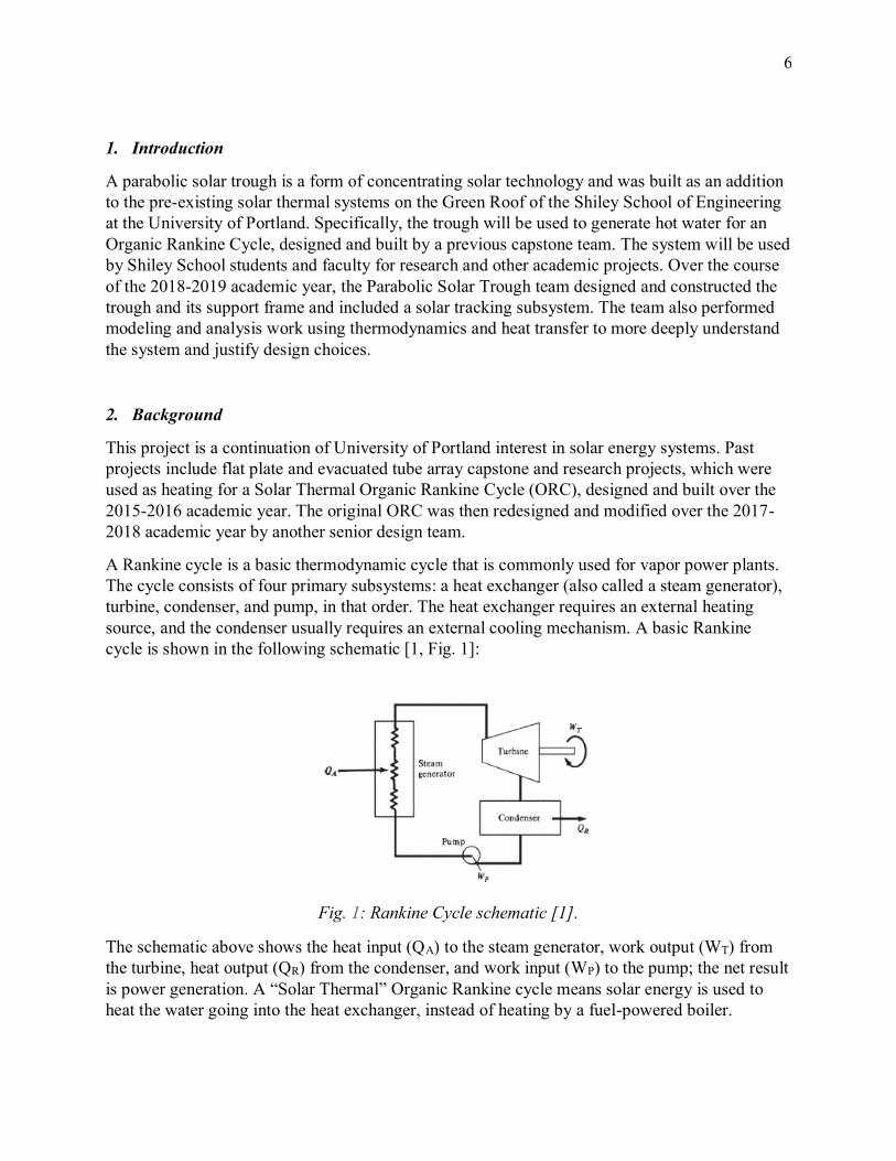
A Rankine cycle is a basic thermodynamic cycle that is commonly used for vapor power plants. The cycle consists of four primary subsystems: a heat exchanger (also called a steam generator), turbine, condenser, and pump, in that order. The heat exchanger requires an external heating source, and the condenser usually requires an external cooling mechanism. A basic Rankine cycle is shown in the following schematic [1, Fig. 1]:

Fig. 1: Rankine Cycle schematic [1].

The schematic above shows the heat input (QA) to the steam generator, work output (WT) from the turbine, heat output (QR) from the condenser, and work input (WP) to the pump; the net result is power generation. A “Solar Thermal” Organic Rankine cycle means solar energy is used to heat the water going into the heat exchanger, instead of heating by a fuel-powered boiler.

7

Currently, for the solar thermal organic Rankine cycle at the University, the ingoing heat is harvested solar energy by a flat plate collector and an array of evacuated tubes. The 2017 team found that they needed an additional heat source for the cycle to run most efficiently. The parabolic trough built by the current capstone team will be added in series with the other solar technologies to fulfill that energy need.

2.1 Existing Technologies of Solar Energy

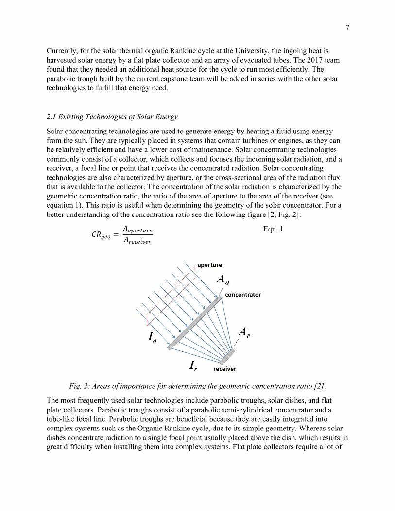
Solar concentrating technologies are used to generate energy by heating a fluid using energy from the sun. They are typically placed in systems that contain turbines or engines, as they can be relatively efficient and have a lower cost of maintenance. Solar concentrating technologies commonly consist of a collector, which collects and focuses the incoming solar radiation, and a receiver, a focal line or point that receives the concentrated radiation. Solar concentrating technologies are also characterized by aperture, or the cross-sectional area of the radiation flux that is available to the collector. The concentration of the solar radiation is characterized by the geometric concentration ratio, the ratio of the area of aperture to the area of the receiver (see equation 1). This ratio is useful when determining the geometry of the solar concentrator. For a better understanding of the concentration ratio see the following figure [2, Fig. 2]:

𝐶𝑅𝑔𝑒𝑜 = 𝐴𝑎𝑝𝑒𝑟𝑡𝑢𝑟𝑒

𝐴𝑟𝑒𝑐𝑒𝑖𝑣𝑒𝑟

Eqn. 1

Fig. 2: Areas of importance for determining the geometric concentration ratio [2].

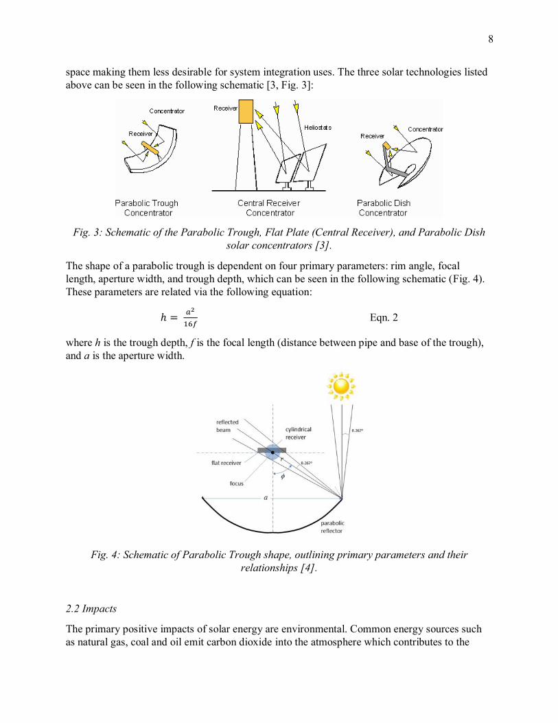
The most frequently used solar technologies include parabolic troughs, solar dishes, and flat plate collectors. Parabolic troughs consist of a parabolic semi-cylindrical concentrator and a tube-like focal line. Parabolic troughs are beneficial because they are easily integrated into complex systems such as the Organic Rankine cycle, due to its simple geometry. Whereas solar dishes concentrate radiation to a single focal point usually placed above the dish, which results in great difficulty when installing them into complex systems. Flat plate collectors require a lot of

8

space making them less desirable for system integration uses. The three solar technologies listed above can be seen in the following schematic [3, Fig. 3]:

Fig. 3: Schematic of the Parabolic Trough, Flat Plate (Central Receiver), and Parabolic Dish

solar concentrators [3].

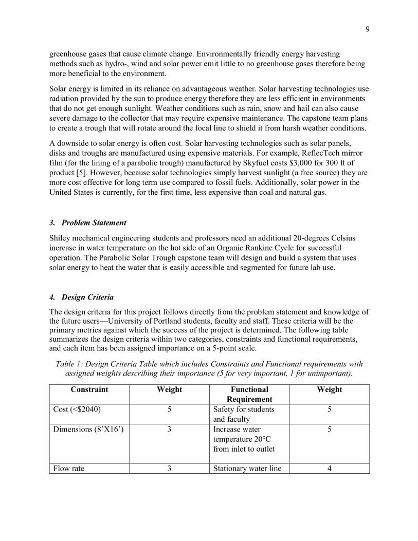
The shape of a parabolic trough is dependent on four primary parameters: rim angle, focal length, aperture width, and trough depth, which can be seen in the following schematic (Fig. 4). These parameters are related via the following equation:

ℎ = 𝑎2

16𝑓 Eqn. 2

where h is the trough depth, f is the focal length (distance between pipe and base of the trough), and a is the aperture width.

Fig. 4: Schematic of Parabolic Trough shape, outlining primary parameters and their

relationships [4].

2.2 Impacts

The primary positive impacts of solar energy are environmental. Common energy sources such as natural gas, coal and oil emit carbon dioxide into the atmosphere which contributes to the

9

greenhouse gases that cause climate change. Environmentally friendly energy harvesting methods such as hydro-, wind and solar power emit little to no greenhouse gases therefore being more beneficial to the environment.

Solar energy is limited in its reliance on advantageous weather. Solar harvesting technologies use radiation provided by the sun to produce energy therefore they are less efficient in environments that do not get enough sunlight. Weather conditions such as rain, snow and hail can also cause severe damage to the collector that may require expensive maintenance. The capstone team plans to create a trough that will rotate around the focal line to shield it from harsh weather conditions.

A downside to solar energy is often cost. Solar harvesting technologies such as solar panels, disks and troughs are manufactured using expensive materials. For example, ReflecTech mirror film (for the lining of a parabolic trough) manufactured by Skyfuel costs $3,000 for 300 ft of product [5]. However, because solar technologies simply harvest sunlight (a free source) they are more cost effective for long term use compared to fossil fuels. Additionally, solar power in the United States is currently, for the first time, less expensive than coal and natural gas.

3. Problem Statement

Shiley mechanical engineering students and professors need an additional 20-degrees Celsius increase in water temperature on the hot side of an Organic Rankine Cycle for successful operation. The Parabolic Solar Trough capstone team will design and build a system that uses solar energy to heat the water that is easily accessible and segmented for future lab use.

4. Design Criteria

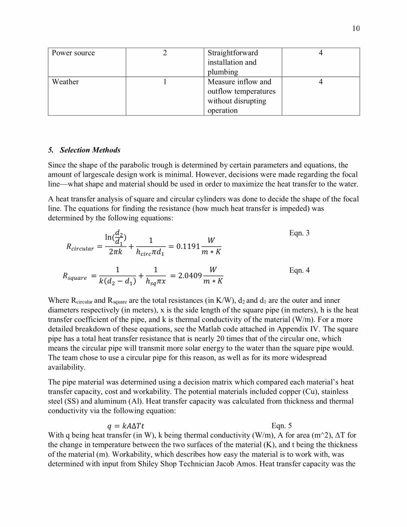
The design criteria for this project follows directly from the problem statement and knowledge of the future users—University of Portland students, faculty and staff. These criteria will be the primary metrics against which the success of the project is determined. The following table summarizes the design criteria within two categories, constraints and functional requirements, and each item has been assigned importance on a 5-point scale.

Table 1: Design Criteria Table which includes Constraints and Functional requirements with assigned weights describing their importance (5 for very important, 1 for unimportant).

Constraint Weight Functional Requirement

Weight

Cost (<$2040) 5 Safety for students and faculty

5

Dimensions (8’X16’) 3 Increase water temperature 20℃ from inlet to outlet

5

Flow rate 3 Stationary water line 4

10

Power source 2 Straightforward installation and plumbing

4

Weather 1 Measure inflow and outflow temperatures without disrupting operation

4

5. Selection Methods

Since the shape of the parabolic trough is determined by certain parameters and equations, the amount of largescale design work is minimal. However, decisions were made regarding the focal line—what shape and material should be used in order to maximize the heat transfer to the water.

A heat transfer analysis of square and circular cylinders was done to decide the shape of the focal line. The equations for finding the resistance (how much heat transfer is impeded) was determined by the following equations:

𝑅𝑐𝑖𝑟𝑐𝑢𝑙𝑎𝑟 =ln (

𝑑2

𝑑1)

2𝜋𝑘+

1

ℎ𝑐𝑖𝑟𝑐𝜋𝑑1 = 0.1191

𝑊

𝑚 ∗ 𝐾

Eqn. 3

𝑅𝑠𝑞𝑢𝑎𝑟𝑒 =1

𝑘(𝑑2 − 𝑑1)+

1

ℎ𝑠𝑞𝜋𝑥 = 2.0409

𝑊

𝑚 ∗ 𝐾

Eqn. 4

Where Rcircular and Rsquare are the total resistances (in K/W), d2 and d1 are the outer and inner diameters respectively (in meters), x is the side length of the square pipe (in meters), h is the heat transfer coefficient of the pipe, and k is thermal conductivity of the material (W/m). For a more detailed breakdown of these equations, see the Matlab code attached in Appendix IV. The square pipe has a total heat transfer resistance that is nearly 20 times that of the circular one, which means the circular pipe will transmit more solar energy to the water than the square pipe would. The team chose to use a circular pipe for this reason, as well as for its more widespread availability.

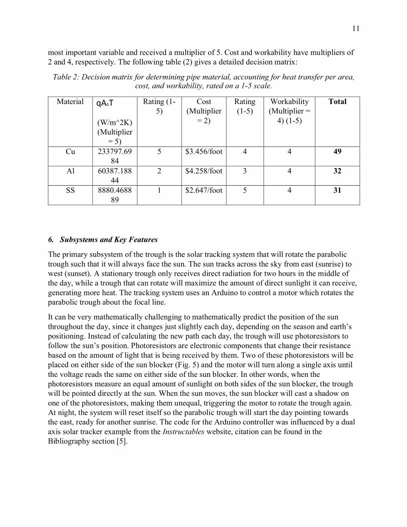
The pipe material was determined using a decision matrix which compared each material’s heat transfer capacity, cost and workability. The potential materials included copper (Cu), stainless steel (SS) and aluminum (Al). Heat transfer capacity was calculated from thickness and thermal conductivity via the following equation:

𝑞 = 𝑘𝐴Δ𝑇𝑡 Eqn. 5 With q being heat transfer (in W), k being thermal conductivity (W/m), A for area (m^2), ΔT for the change in temperature between the two surfaces of the material (K), and t being the thickness of the material (m). Workability, which describes how easy the material is to work with, was determined with input from Shiley Shop Technician Jacob Amos. Heat transfer capacity was the

11

most important variable and received a multiplier of 5. Cost and workability have multipliers of 2 and 4, respectively. The following table (2) gives a detailed decision matrix:

Table 2: Decision matrix for determining pipe material, accounting for heat transfer per area, cost, and workability, rated on a 1-5 scale.

Material qA∆T

(W/m^2K) (Multiplier

= 5)

Rating (1-5)

Cost (Multiplier

= 2)

Rating (1-5)

Workability (Multiplier =

4) (1-5)

Total

Cu 233797.6984

5 $3.456/foot 4 4 49

Al 60387.18844

2 $4.258/foot 3 4 32

SS 8880.468889

1 $2.647/foot 5 4 31

6. Subsystems and Key Features

The primary subsystem of the trough is the solar tracking system that will rotate the parabolic trough such that it will always face the sun. The sun tracks across the sky from east (sunrise) to west (sunset). A stationary trough only receives direct radiation for two hours in the middle of the day, while a trough that can rotate will maximize the amount of direct sunlight it can receive, generating more heat. The tracking system uses an Arduino to control a motor which rotates the parabolic trough about the focal line.

It can be very mathematically challenging to mathematically predict the position of the sun throughout the day, since it changes just slightly each day, depending on the season and earth’s positioning. Instead of calculating the new path each day, the trough will use photoresistors to follow the sun’s position. Photoresistors are electronic components that change their resistance based on the amount of light that is being received by them. Two of these photoresistors will be placed on either side of the sun blocker (Fig. 5) and the motor will turn along a single axis until the voltage reads the same on either side of the sun blocker. In other words, when the photoresistors measure an equal amount of sunlight on both sides of the sun blocker, the trough will be pointed directly at the sun. When the sun moves, the sun blocker will cast a shadow on one of the photoresistors, making them unequal, triggering the motor to rotate the trough again. At night, the system will reset itself so the parabolic trough will start the day pointing towards the east, ready for another sunrise. The code for the Arduino controller was influenced by a dual axis solar tracker example from the Instructables website, citation can be found in the Bibliography section [5].

12

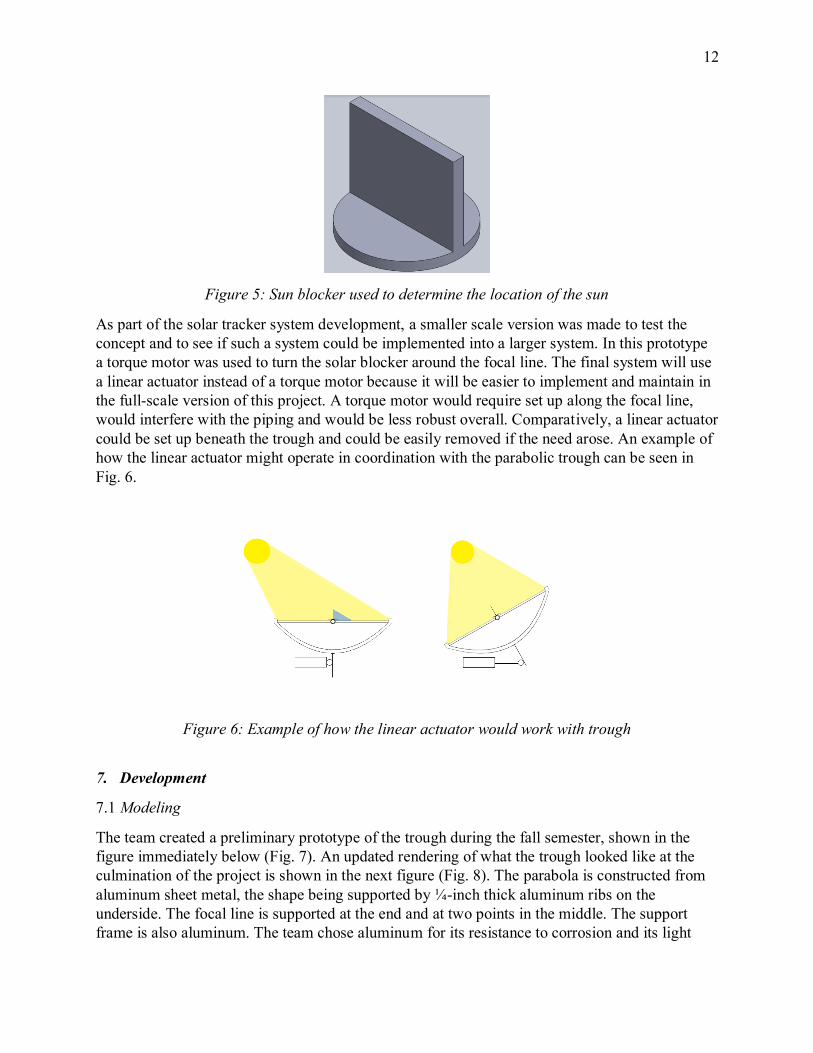
Figure 5: Sun blocker used to determine the location of the sun

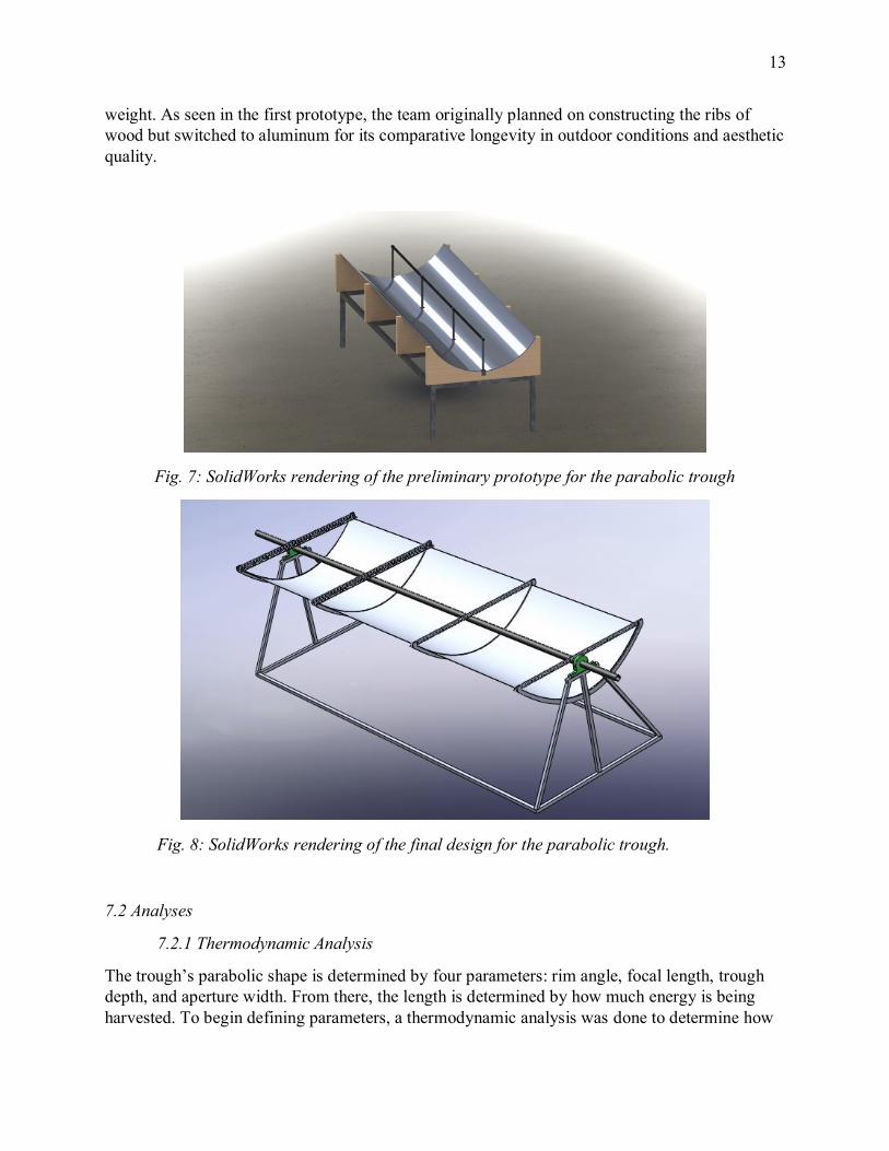
As part of the solar tracker system development, a smaller scale version was made to test the concept and to see if such a system could be implemented into a larger system. In this prototype a torque motor was used to turn the solar blocker around the focal line. The final system will use a linear actuator instead of a torque motor because it will be easier to implement and maintain in the full-scale version of this project. A torque motor would require set up along the focal line, would interfere with the piping and would be less robust overall. Comparatively, a linear actuator could be set up beneath the trough and could be easily removed if the need arose. An example of how the linear actuator might operate in coordination with the parabolic trough can be seen in Fig. 6.

Figure 6: Example of how the linear actuator would work with trough

7. Development

7.1 Modeling

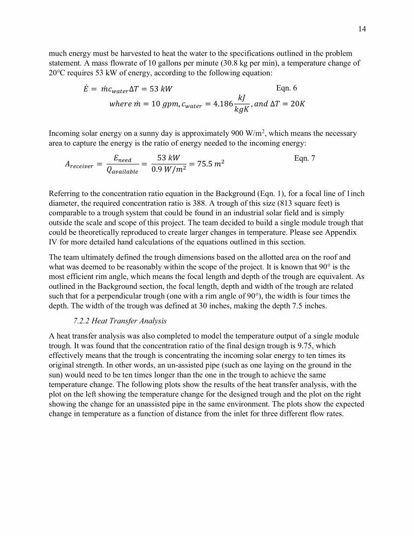
The team created a preliminary prototype of the trough during the fall semester, shown in the figure immediately below (Fig. 7). An updated rendering of what the trough looked like at the culmination of the project is shown in the next figure (Fig. 8). The parabola is constructed from aluminum sheet metal, the shape being supported by ¼-inch thick aluminum ribs on the underside. The focal line is supported at the end and at two points in the middle. The support frame is also aluminum. The team chose aluminum for its resistance to corrosion and its light

13

weight. As seen in the first prototype, the team originally planned on constructing the ribs of wood but switched to aluminum for its comparative longevity in outdoor conditions and aesthetic quality.

Fig. 7: SolidWorks rendering of the preliminary prototype for the parabolic trough

Fig. 8: SolidWorks rendering of the final design for the parabolic trough.

7.2 Analyses

7.2.1 Thermodynamic Analysis

The trough’s parabolic shape is determined by four parameters: rim angle, focal length, trough depth, and aperture width. From there, the length is determined by how much energy is being harvested. To begin defining parameters, a thermodynamic analysis was done to determine how

14

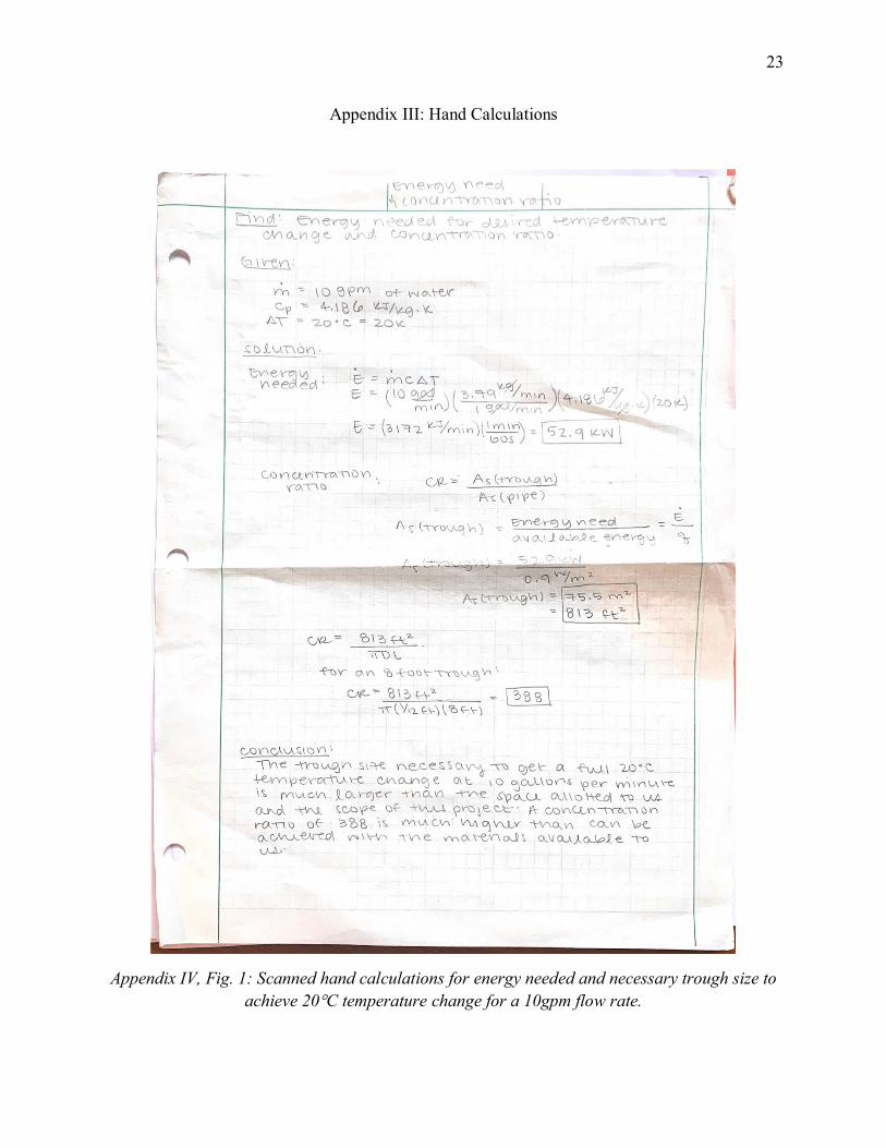
much energy must be harvested to heat the water to the specifications outlined in the problem statement. A mass flowrate of 10 gallons per minute (30.8 kg per min), a temperature change of 20℃ requires 53 kW of energy, according to the following equation:

�̇� = �̇�𝑐𝑤𝑎𝑡𝑒𝑟∆𝑇 = 53 𝑘𝑊 Eqn. 6

𝑤ℎ𝑒𝑟𝑒 �̇� = 10 𝑔𝑝𝑚, 𝑐𝑤𝑎𝑡𝑒𝑟 = 4.186𝑘𝐽

𝑘𝑔𝐾, 𝑎𝑛𝑑 ∆𝑇 = 20𝐾

Incoming solar energy on a sunny day is approximately 900 W/m2, which means the necessary area to capture the energy is the ratio of energy needed to the incoming energy:

𝐴𝑟𝑒𝑐𝑒𝑖𝑣𝑒𝑟 = 𝐸𝑛𝑒𝑒𝑑

𝑄𝑎𝑣𝑎𝑖𝑙𝑎𝑏𝑙𝑒=

53 𝑘𝑊

0.9 𝑊/𝑚2= 75.5 𝑚2

Eqn. 7

Referring to the concentration ratio equation in the Background (Eqn. 1), for a focal line of 1inch diameter, the required concentration ratio is 388. A trough of this size (813 square feet) is comparable to a trough system that could be found in an industrial solar field and is simply outside the scale and scope of this project. The team decided to build a single module trough that could be theoretically reproduced to create larger changes in temperature. Please see Appendix IV for more detailed hand calculations of the equations outlined in this section.

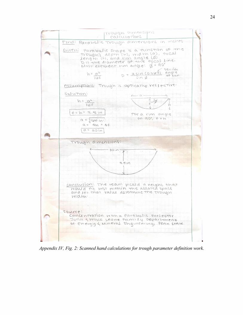
The team ultimately defined the trough dimensions based on the allotted area on the roof and what was deemed to be reasonably within the scope of the project. It is known that 90° is the most efficient rim angle, which means the focal length and depth of the trough are equivalent. As outlined in the Background section, the focal length, depth and width of the trough are related such that for a perpendicular trough (one with a rim angle of 90°), the width is four times the depth. The width of the trough was defined at 30 inches, making the depth 7.5 inches.

7.2.2 Heat Transfer Analysis

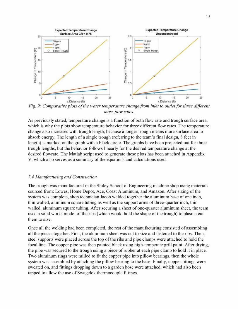
A heat transfer analysis was also completed to model the temperature output of a single module trough. It was found that the concentration ratio of the final design trough is 9.75, which effectively means that the trough is concentrating the incoming solar energy to ten times its original strength. In other words, an un-assisted pipe (such as one laying on the ground in the sun) would need to be ten times longer than the one in the trough to achieve the same temperature change. The following plots show the results of the heat transfer analysis, with the plot on the left showing the temperature change for the designed trough and the plot on the right showing the change for an unassisted pipe in the same environment. The plots show the expected change in temperature as a function of distance from the inlet for three different flow rates.

15

Fig. 9: Comparative plots of the water temperature change from inlet to outlet for three different

mass flow rates.

As previously stated, temperature change is a function of both flow rate and trough surface area, which is why the plots show temperature behavior for three different flow rates. The temperature change also increases with trough length, because a longer trough means more surface area to absorb energy. The length of a single trough (referring to the team’s final design, 8 feet in length) is marked on the graph with a black circle. The graphs have been projected out for three trough lengths, but the behavior follows linearly for the desired temperature change at the desired flowrate. The Matlab script used to generate these plots has been attached in Appendix V, which also serves as a summary of the equations and calculations used.

7.4 Manufacturing and Construction

The trough was manufactured in the Shiley School of Engineering machine shop using materials sourced from: Lowes, Home Depot, Ace, Coast Aluminum, and Amazon. After sizing of the system was complete, shop technician Jacob welded together the aluminum base of one inch, thin walled, aluminum square tubing as well as the support arms of three-quarter inch, thin walled, aluminum square tubing. After securing a sheet of one-quarter aluminum sheet, the team used a solid works model of the ribs (which would hold the shape of the trough) to plasma cut them to size.

Once all the welding had been completed, the rest of the manufacturing consisted of assembling all the pieces together. First, the aluminum sheet was cut to size and fastened to the ribs. Then, steel supports were placed across the top of the ribs and pipe clamps were attached to hold the focal line. The copper pipe was then painted black using high-temperate grill paint. After drying, the pipe was secured to the trough using a piece of rubber at each pipe clamp to hold it in place. Two aluminum rings were milled to fit the copper pipe into pillow bearings, then the whole system was assembled by attaching the pillow bearing to the base. Finally, copper fittings were sweated on, and fittings dropping down to a garden hose were attached, which had also been tapped to allow the use of Swagelok thermocouple fittings.

16

7.5 Testing

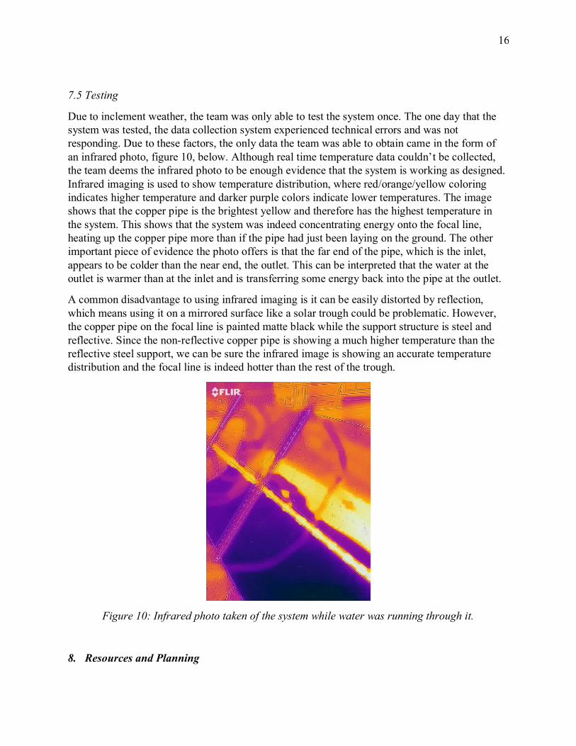
Due to inclement weather, the team was only able to test the system once. The one day that the system was tested, the data collection system experienced technical errors and was not responding. Due to these factors, the only data the team was able to obtain came in the form of an infrared photo, figure 10, below. Although real time temperature data couldn’t be collected, the team deems the infrared photo to be enough evidence that the system is working as designed. Infrared imaging is used to show temperature distribution, where red/orange/yellow coloring indicates higher temperature and darker purple colors indicate lower temperatures. The image shows that the copper pipe is the brightest yellow and therefore has the highest temperature in the system. This shows that the system was indeed concentrating energy onto the focal line, heating up the copper pipe more than if the pipe had just been laying on the ground. The other important piece of evidence the photo offers is that the far end of the pipe, which is the inlet, appears to be colder than the near end, the outlet. This can be interpreted that the water at the outlet is warmer than at the inlet and is transferring some energy back into the pipe at the outlet.

A common disadvantage to using infrared imaging is it can be easily distorted by reflection, which means using it on a mirrored surface like a solar trough could be problematic. However, the copper pipe on the focal line is painted matte black while the support structure is steel and reflective. Since the non-reflective copper pipe is showing a much higher temperature than the reflective steel support, we can be sure the infrared image is showing an accurate temperature distribution and the focal line is indeed hotter than the rest of the trough.

Figure 10: Infrared photo taken of the system while water was running through it.

8. Resources and Planning

17

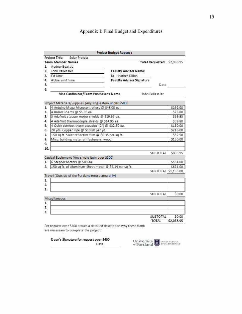
The primary resources of interest for this project included space, funding, and necessary personnel. In June of 2018 the team submitted a funding request for $2,039, which was fulfilled by funding from the Glarneau Fund. A detailed breakdown of the budget is attached in Appendix I as well as a final expenditures report. The most expensive portion of the project was the solar tracking system, which required multiple stepper motors, Arduino microcontrollers, bread boards, and Adafruit stepper motor shields that interface between the motor and microcontroller. The other capital equipment item was aluminum material, which was used to form the parabolic dishes and was chosen for its flexibility and resistance to corrosion. The water flows through copper pipes, which were chosen for their high heat conductivity. Thermocouples are also used to monitor temperature change within the system. Refer to Appendix I for more detail.

The project primarily took place on the Shiley Green Roof. The team used Shiley Room 246 for storage and meeting space.

The necessary personnel for the project included the team members, project advisor and Shiley shop faculty. The team consisted of four senior mechanical engineering students, each with unique skills and responsibilities within the team. Audrey Beattie acted as team lead, keeping track of meetings and communication between the team and outside personnel. Abbie Smithline was the final editor of all documents and deliverables, ensuring they are acceptable for submission. Ed Lane took lead on the tracking system, and ensured the team is staying on track with deliverable deadlines. John Pellessier was the budget coordinator and card holder. The faculty member advising this project was Dr. Dillon, who also worked with the past year’s Organic Rankine Cycle team as well as the previous solar power teams. The team also received support from technicians in the Shiley machine shop: Jacob Amos, Jared Rees, Allen Hansen, and Christina Chrestatos.

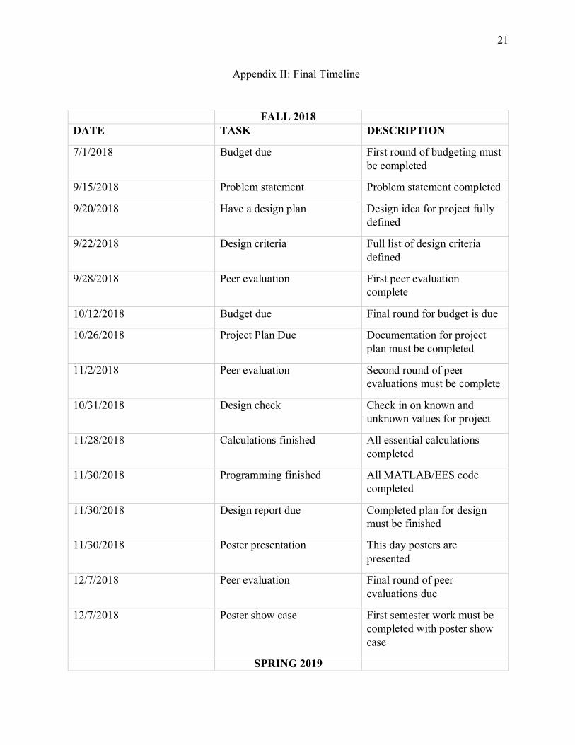
The project timeline for the fall and spring semesters is outlined in Appendix II and details the important dates for the project. This table includes completion dates starting with the first round of funding in the summer through the team presentation on Founder’s Day in the spring and the due date of the final design report. This schedule includes due dates assigned for the capstone class such as Peer Evaluation dates and the Poster Show Case. It also includes important dates for the group itself such as completion of MATLAB code, and for fabrication and testing of the final product.

9. Conclusion

9.1 Project Summary

The Solar Parabolic Trough project concludes with a single trough that is eight feet in length and is outfitted with a passive data collection system and a solar tracker. Although the team was not able to produce real time temperature data due to weather constraints, the team was able to see the trough in action via infrared imaging. The scope of the project was adjusted from its original conception, but the team remains satisfied with what they were able to accomplish given the constraints and scope of the project. The project was an excellent learning opportunity for the team, particularly for understanding the design process and how to communicate with immediate team members and outside stakeholders.

18

9.2 Future Work

Following the completion of the solar parabolic trough, the team has made a list of future improvements and work that could be done to improve the efficacy and design of the trough. Since the weather was not suitable for properly testing the trough, the first priority should be testing. Testing could be completed either in the early fall or during the summer when there is an optimum amount of solar radiation emitted by the sun. After testing is completed, a reflective film or polish could be added to the trough to increase the amount of light that is focused on the focal line. After the reflective film or polish is applied, another round of testing should be done. The two sets of data (with and without the film), should be compared and the superior design should be implemented for all future solar parabolic troughs. These improvements could be completed by future capstone teams or student researchers attending the University of Portland.

Bibliography

[1] P. Kiameh, “Chapter 2: Steam Power Plants from the Power Generation Handbook: Selection, Applications, Operation and Maintenance,” IEEE Engineering 360. [Online]. Available: https://www.globalspec.com/reference/73481/203279/chapter-2-steam-power-plants [Accessed: 25 Oct. 2018].

[2] M. Fedkin, “Utility Solar Power and Concentration: Concentration Ratio,” John and Willie Leone Family Department of Energy and Mineral Engineering. [Online]. Available: https://www.e-education.psu.edu/eme812/node/8 [Accessed: 25 Oct. 2018].

[3] “Power from the Sun: Solar Energy System Design,” [Online]. Available: http://www.powerfromthesun.net/Book/chapter01/chapter01.html [Accessed: 25 Oct. 2018].

[4] Mark Fedkin, modified after Duffie and Beckman, “2.4 Concentration with a Parabolic Reflector,” John and Willie Leone Family Department of Energy and Mineral Engineering at Penn State, 2013. https://www.e-education.psu.edu/eme812/node/557

[5] “SkyFuel: ReflecTech: The World’s Leading High Reflective Film for Outdoor Solar Applications,” [Online]. Available: http://www.skyfuel.com/products/reflectech/ [Accessed: 2 Dec. 2018]

[5] Instructables. “Simple Dual Axis Solar Tracker.” Instructables, BrownDogGadgets, 10 Oct. 2017, www.instructables.com/id/Simple-Dual-Axis-Solar-Tracker/.

19

Appendix I: Final Budget and Expenditures

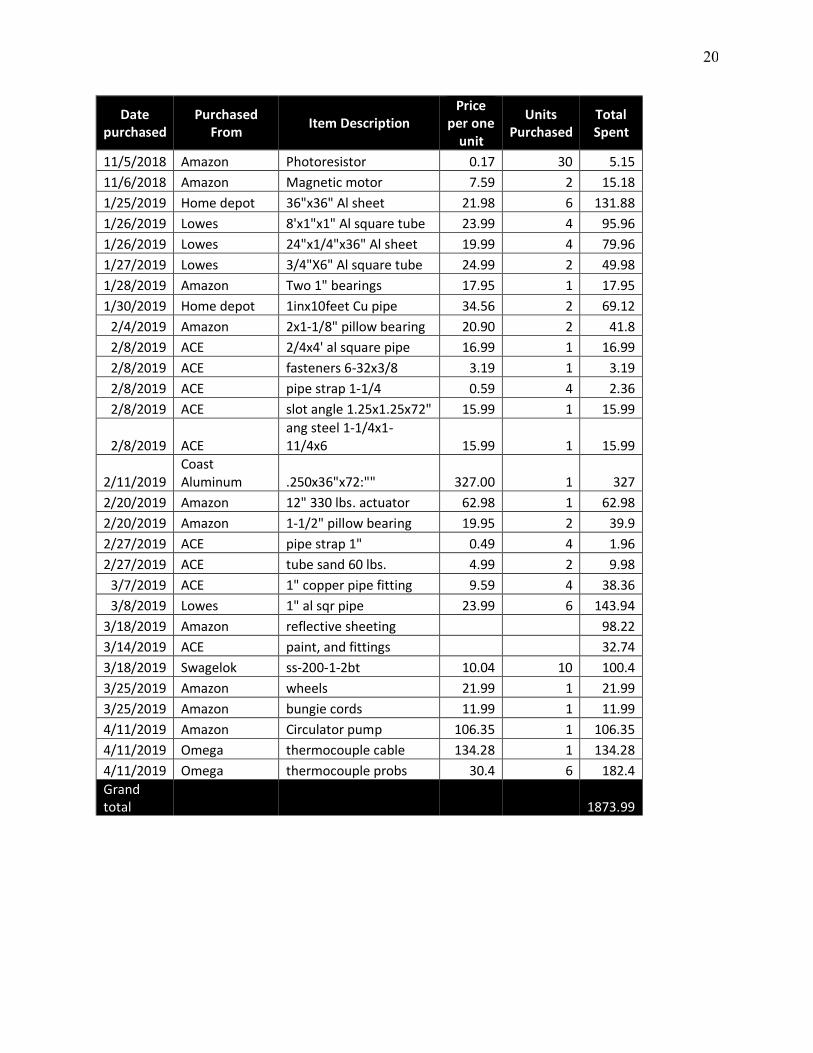
20

Date purchased

Purchased From

Item Description Price

per one unit

Units Purchased

Total Spent

11/5/2018 Amazon Photoresistor 0.17 30 5.15

11/6/2018 Amazon Magnetic motor 7.59 2 15.18

1/25/2019 Home depot 36"x36" Al sheet 21.98 6 131.88

1/26/2019 Lowes 8'x1"x1" Al square tube 23.99 4 95.96

1/26/2019 Lowes 24"x1/4"x36" Al sheet 19.99 4 79.96

1/27/2019 Lowes 3/4"X6" Al square tube 24.99 2 49.98

1/28/2019 Amazon Two 1" bearings 17.95 1 17.95

1/30/2019 Home depot 1inx10feet Cu pipe 34.56 2 69.12

2/4/2019 Amazon 2x1-1/8" pillow bearing 20.90 2 41.8

2/8/2019 ACE 2/4x4' al square pipe 16.99 1 16.99

2/8/2019 ACE fasteners 6-32x3/8 3.19 1 3.19

2/8/2019 ACE pipe strap 1-1/4 0.59 4 2.36

2/8/2019 ACE slot angle 1.25x1.25x72" 15.99 1 15.99

2/8/2019 ACE ang steel 1-1/4x1-11/4x6 15.99 1 15.99

2/11/2019 Coast Aluminum .250x36"x72:"" 327.00 1 327

2/20/2019 Amazon 12" 330 lbs. actuator 62.98 1 62.98

2/20/2019 Amazon 1-1/2" pillow bearing 19.95 2 39.9

2/27/2019 ACE pipe strap 1" 0.49 4 1.96

2/27/2019 ACE tube sand 60 lbs. 4.99 2 9.98

3/7/2019 ACE 1" copper pipe fitting 9.59 4 38.36

3/8/2019 Lowes 1" al sqr pipe 23.99 6 143.94

3/18/2019 Amazon reflective sheeting 98.22

3/14/2019 ACE paint, and fittings 32.74

3/18/2019 Swagelok ss-200-1-2bt 10.04 10 100.4

3/25/2019 Amazon wheels 21.99 1 21.99

3/25/2019 Amazon bungie cords 11.99 1 11.99

4/11/2019 Amazon Circulator pump 106.35 1 106.35

4/11/2019 Omega thermocouple cable 134.28 1 134.28

4/11/2019 Omega thermocouple probs 30.4 6 182.4

Grand total 1873.99

21

Appendix II: Final Timeline

FALL 2018

DATE TASK DESCRIPTION

7/1/2018 Budget due First round of budgeting must be completed

9/15/2018 Problem statement Problem statement completed

9/20/2018 Have a design plan Design idea for project fully defined

9/22/2018 Design criteria Full list of design criteria defined

9/28/2018 Peer evaluation First peer evaluation complete

10/12/2018 Budget due Final round for budget is due

10/26/2018 Project Plan Due Documentation for project plan must be completed

11/2/2018 Peer evaluation Second round of peer evaluations must be complete

10/31/2018 Design check Check in on known and unknown values for project

11/28/2018 Calculations finished All essential calculations completed

11/30/2018 Programming finished All MATLAB/EES code completed

11/30/2018 Design report due Completed plan for design must be finished

11/30/2018 Poster presentation This day posters are presented

12/7/2018 Peer evaluation Final round of peer evaluations due

12/7/2018 Poster show case First semester work must be completed with poster show case

SPRING 2019

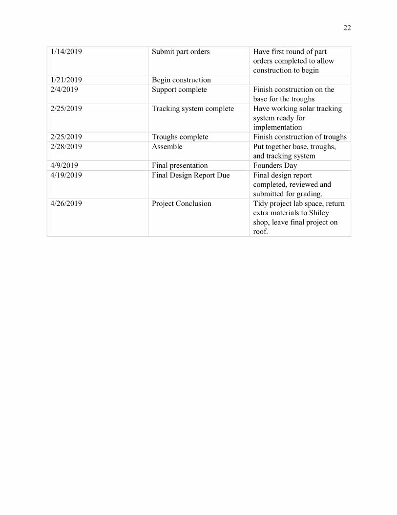
22

1/14/2019 Submit part orders Have first round of part orders completed to allow construction to begin

1/21/2019 Begin construction 2/4/2019 Support complete Finish construction on the

base for the troughs 2/25/2019 Tracking system complete Have working solar tracking

system ready for implementation

2/25/2019 Troughs complete Finish construction of troughs 2/28/2019 Assemble Put together base, troughs,

and tracking system 4/9/2019 Final presentation Founders Day 4/19/2019 Final Design Report Due Final design report

completed, reviewed and submitted for grading.

4/26/2019 Project Conclusion Tidy project lab space, return extra materials to Shiley shop, leave final project on roof.

23

Appendix III: Hand Calculations

Appendix IV, Fig. 1: Scanned hand calculations for energy needed and necessary trough size to

achieve 20C temperature change for a 10gpm flow rate.

24

Appendix IV, Fig. 2: Scanned hand calculations for trough parameter definition work.

25

Appendix IV: Matlab Code

%ME Capstone: Expected Water Temperature Data %Audrey Beattie

clear all close all

%Find: show temperature behavior as a function of the length of the pipe %and flow rate.

%Assumptions: %Constant cp of water %Constant and uniform heat flux over pipe %Steady state %Incompressible liquid %No evaporation %Free convection on the outside of the pipe is negligible

%Given: Do = 2.8575E-2; %m outer dia of pipe Di = 2.6035E-2; %m inner dia of pipe q = 800; %W/m^2 heat flux from sun cp = 4.184; %kJ/kg*K specific heat of water a = 30*2.54E-2; f = 7.5*2.54E-2; A1 = ((a/2)*sqrt(1+(a^2/(16*f^2))) + 2*f*log((a/(4*f)) + sqrt(1 +

(a^2/(16*f^2)))))

C1 = A1/(pi*Do); %C1 = more complicated concentration ratio, surface area

of trough/surface area of pipe C2 = a/(pi*Do); %C2 = 'geometric concentration ratio', apeture/surface

area of pipe qconc1 = q*C1 qconc2 = q*C2

%Solution: %q(pi/4)(do^2-di^2)L = mcp(delT)

delTnon = @(x,m) q*(pi/4).*(Do^2 - Di^2).*x./(m.*cp); delTconc1 = @(x,m) qconc1*(pi/4).*(Do^2 - Di^2).*x./(m.*cp); delTconc2 = @(x,m) qconc2*(pi/4).*(Do^2 - Di^2).*x./(m.*cp);

%various flow rate convert = 0.063; %kg/s per gal/min of water m10 = 10*convert; m7 = 10*convert; m5 = 5*convert; m3 = 3*convert; m1 = 1*convert;

%plot solution %1 meter = 3.28 ft x = linspace(0,24);

26

xmeters = x./3.28; figure(1) plot(x, delTnon(x,m10), x, delTnon(x,m5), x, delTnon(x,m1)); legend('10 gpm',

'5 gpm', '1 gpm'); title('Unconcentrated'); xlabel('x (m)'), ylabel('delta

T')

%plot unconcentrated temperature change figure(2) plot(x, delTnon(xmeters,m10), x, delTnon(xmeters,m5), x, delTnon(xmeters,m1),

'LineWidth',2); hold on plot(8, delTnon(8./3.28,m10), 'ko', 8, delTnon(8./3.28,m5),'ko', 8,

delTnon(8./3.28,m1),'ko') legend('10 gpm', '5 gpm', '1 gpm', 'Single Trough'); title ({'Expected Temperature Change';'Unconcentrated'}); xlabel('x Distance

(ft)'); ylabel('Change in Temperature (C)');

%plot 9.75 concentration ratio figure(3) plot(x, delTconc1(xmeters,m10), x, delTconc1(xmeters,m5), x,

delTconc1(xmeters,m1), 'LineWidth', 2) hold on plot(8, delTconc1(8./3.28, m10), 'ko', 8, delTconc1(8./3.28,m5), 'ko', 8,

delTconc1(8./3.28,m1), 'ko') legend('10 gpm', '5 gpm', '1 gpm', 'Single Trough'); title({'Expected Temperature Change';'Surface Area CR = 9.75'}); xlabel('x

Distance (ft)'); ylabel('Change in Temperature (C)');

%plot 8.5 concentration ratio figure(4) plot(x, delTconc2(xmeters,m10), x, delTconc2(xmeters,m5), x,

delTconc2(xmeters,m1)) hold on plot(8, delTconc2(8./3.28, m10), 'ko', 8, delTconc2(8./3.28,m5), 'ko', 8,

delTconc2(8./3.28,m1), 'ko'); legend('10 gpm', '5 gpm', '1 gpm', 'Single Trough'); title ({'Expected Temperature Change';'Geometric CR = 8.5'}); xlabel('x

Distance (ft)'); ylabel('Change in Temperature (C)');

Copy of Matlab Script used to generate Heat Transfer model plots.

27

%% constants / given

Voldot=600 %mL/sec

oD=0.015875 %m

iD=0.0144526 %m

mu=855E-6 %mNs/m^2

rho=1000 %kg/m^3

kh2o=613e-3 % w/m*K

kcu=401 % w/m*K

mLtm3=1e-6 %m^3/mL

Nucirc=4.36 %assuming constatns Ts

Nusqr=3.61 %assuming constatns Ts

%%calculated values

Vel=Voldot*(mLtm3)/(pi/4*iD^2) %m/sec

acirc=pi/4*iD^2 %m^2 area circulr pipe

x=sqrt(acirc) %m side length of sqare pipe

Rcirc=Vel*iD/(mu/rho) %Re

Rsqaure=Vel*x/(mu/rho) %Re

hcirc=Nucirc*kh2o/iD %w/m^2*K

hsqr=Nusqr*kh2o/(4*x^2/(2*x)) %w/m^2*K

Rtotcirc=log(oD/iD)/(2*pi*kcu)+1/(hcirc*pi*iD) %w/m*K

Rtotsqr=1/(kcu*(oD-iD))+1/(hsqr*pi*x) %w/m*K

Copy of Matlab script used to calculate resistances given in Eqns. 2 and 3.