Paradoxes and Mechanisms for Choice under Risk

By James C. Cox, Vjollca Sadiraj, and Ulrich Schmidt

Forthcoming in Experimental Economics

1

Paradoxes and Mechanisms for Choice under Risk

By James C. Cox, Vjollca Sadiraj, and Ulrich Schmidt1

Abstract: Experiments on choice under risk typically involve multiple decisions by

individual subjects. The choice of mechanism for selecting decision(s) for payoff is an

essential design feature unless subjects isolate each one of the multiple decisions. We report

treatments with different payoff mechanisms but the same decision tasks. The data show large

differences across mechanisms in subjects’ revealed risk preferences, a clear violation of

isolation. We illustrate the importance of these mechanism effects by identifying their

implications for classical tests of theories of decision under risk. We discuss theoretical

properties of commonly used mechanisms, and new mechanisms introduced herein, in order

to clarify which mechanisms are theoretically incentive compatible for which theories. We

identify behavioral properties of some mechanisms that can introduce bias in elicited risk

preferences – from cross-task contamination – even when the mechanism used is theoretically

incentive compatible. We explain that selection of a payoff mechanism is an important

component of experimental design in many topic areas including social preferences, public

goods, bargaining, and choice under uncertainty and ambiguity as well as experiments on

decisions under risk.

Keywords: payoff mechanisms, incentive compatibility, experiments,

cross-task contamination, paradoxes

JEL classifications: C90, D80

1 Introduction

Most experiments on choice under risk involve multiple decisions by individual subjects. This

necessitates choice of a mechanism for determining incentive payments to the subjects.

Mechanisms used in papers published by top five general readership journals and a prominent

field journal vary quite widely from “paying all decisions sequentially” to “paying all

decisions at the end” to “randomly paying one decision for each subject” to “randomly paying

a few decisions for each subject” to “randomly paying some of the subjects” to “randomly

paying one of the subjects” to “rank-based payment” to “no payment” to unidentified

1 Financial support was provided by the National Science Foundation (grant number SES-0849590) and the Fritz

Thyssen Stiftung. Valuable comments and suggestions were provided by Glenn Harrison, the referees and an

editor.

2

mechanisms.2 This raises questions about whether different payoff mechanisms elicit different

data in otherwise identical experimental treatments and, if so, whether these mechanism

effects have significant implications for conclusions drawn from data. We report an

experiment with several payoff mechanisms that directly addresses these questions. Data from

our experiment show that subjects’ revealed risk preferences differ across mechanisms. We

illustrate the importance of these payoff mechanism effects by using data from alternative

mechanisms to test for consistency with classic paradoxes designed to challenge theories of

decision under risk.

We provide an explanation of theoretical incentive compatibility or incompatibility of

alternative mechanisms for prominent decision theories. Data from our experiments are used

to identify mechanism biases in risk preference elicitation such as choice-order effects and

other types of cross-task contamination in which a subject’s choice in one decision task may

be affected by the choices made in some other tasks.

Issues of mechanism incentive incompatibility and cross-task contamination are not

confined to experiments on risk aversion. We explain that the payoff mechanism effects have

implications for experiments in many other topic areas including social preferences, public

goods, bargaining, and choice under uncertainty and ambiguity.

2 Classic properties of theories of decision under risk

Allais (1953) raised an objection to the independence axiom of expected utility theory (EU)

by constructing thought experiments that seem to imply paradoxical outcomes. Subsequent

behavioral experiments focused on two patterns that are incompatible with the independence

axiom: the common ratio effect (CRE) and common consequence effect (CCE). As we shall

explain, some of the lottery pairs used in our experiment were selected because they make it

possible to observe CRE and CCE if they characterize experimental subjects’ revealed risk

preferences.

Yaari (1987) introduced the dual independence axiom and constructed an alternative

theory to EU with functional that is nonlinear in probabilities (unless the agent is risk neutral)

and linear in payoffs (for all risk attitudes). The dual common ratio effect (DCRE) and dual

common consequence effect (DCCE) are the dual analogs of CRE and CCE. Some of the

2 Mechanisms used are reported in Table 1 of Azrieli et al. (2013) for papers published in 2011 in American

Economic Review, Econometrica, Journal of Political Economy, Review of Economic Studies, Quarterly Journal

of Economics, and Experimental Economics.

3

lottery pairs used in our experiment were designed to make it possible to observe DCRE and

DCCE if they characterize experimental subjects’ revealed risk preferences.

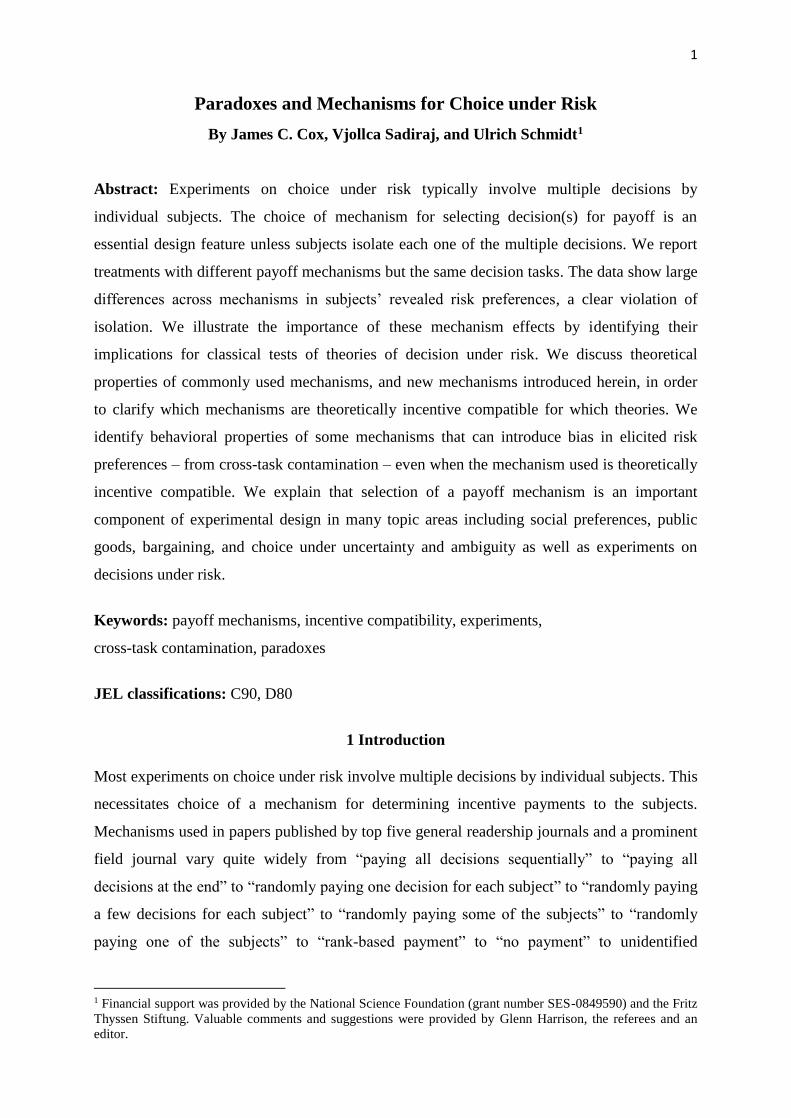
The five pairs of lotteries used in our experiment are portrayed in Table 1. The left-

most column lists the lottery pair numbers and the top row shows bingo ball numbers that

determine lottery payoffs. The dollar amounts of payoffs are reported in the table.

Probabilities of those payoffs are represented in two ways, by the widths of the rectangles

containing the dollar amounts and by the ratios of the number of bingo balls that generate

those payoffs to the total number of 20 bingo balls. For example, the less risky (S) lottery in

Pair 4 pays $6 with probability 1/4 (5 balls/20 balls) or $12 with probability 3/4 (15 balls/20

balls). The more risky lottery (R) in Pair 4 pays $0 with probability 1/20 (1 ball/20 balls) or

$10 with probability 1/5 (4 balls/20 balls) or $12 with probability 3/4 (15 balls/20 balls).

Table 1. Lottery Pairs Used in the Experiment

Less Risky (S) More Risky (R)

Pair\Ball Nr. 1-5 6-15 16-20 1 2-4 5 6-16 17-20

1 $0 $3 $0 $5

2 $6 $0 $10

3 $0 $6 $0 $10

4 $6 $12 0 $10 $12

5 $18 $12 $22

A test for CRE uses two lottery pairs where the lotteries in one pair (Pair 3 in Table 1)

are constructed from the lotteries in the other pair (Pair 2 in Table 1) by multiplying all

probabilities by a common factor (1/4 in our study) and assigning the remaining probability to

a common outcome ($0 in our study). It follows from linearity in probabilities of the expected

utility functional that an expected utility agent would choose either the less risky lotteries in

both pairs or the riskier ones.3 Any mixed choices of the riskier and the less risky lottery

across Pairs 2 and 3 reveals CRE.

A test for CCE also uses two lottery pairs. Here, the lotteries in one pair (Pair 4 in

Table 1) are constructed from the lotteries in another pair (Pair 3 in Table 1) by shifting

probability mass (75% in our study) from one common outcome ($0 in our study) to a

different common outcome ($12 in our study). It is easy to verify that expected utility theory

requires that either the less risky lotteries be chosen in both pairs or the riskier ones be chosen

in both pairs. Any mixture of the riskier and the less risky lotteries across Pairs 3 and 4

reveals CCE.

3 Within any pair of lotteries, we call the less risky (resp. riskier) lottery the one with the smaller (resp. larger)

variance.

4

The null hypotheses that follow from the independence axiom of expected utility

theory are that the proportion of choices of the less risky option in Pair 3 should be the same

as the proportions of choices of the less risky options in Pairs 2 and 4:

Hypothesis 1: The proportions of choices of the less risky option are the same for Pair

2 and Pair 3 (absence of CRE).

Hypothesis 2: The proportions of choices of the less risky option are the same for Pair

3 and Pair 4 (absence of CCE).

One-sided alternatives to the above hypotheses are provided by fanning-out (Machina 1982)

and fanning-in (Neilson, 1992). Subjects’ revealed risk preferences under each mechanism

can be used to test these hypotheses.

DCRE and DCCE play the same role for dual theory of expected utility (Yaari 1987)

as CRE and CCE do for expected utility theory. Because the dual theory functional is linear in

payoffs, it exhibits constant absolute and constant relative risk aversion. Consequently, neither

multiplying all outcomes in a lottery pair by the same factor (DCRE: see Pairs 1 and 3 in

Table 1, the multiplier is 2) nor adding a constant to all outcomes in a lottery pair (DCCE: see

Pairs 2 and 5 where the constant equals $12) affects choices. Yaari (1987) stated that the dual

paradoxes could be used to refute his theory analogously to the way in which CRE and CCE

had been used to refute expected utility theory. As far as we know, however, the dual

paradoxes have never been investigated in a systematic empirical test with a theoretically

incentive compatible mechanism.

The null hypotheses that follow from the dual independence axiom (which implies

linearity in payoffs) are that the proportion of choices of the less risky option should be: (a)

the same in Pairs 1 and 3; and (b) the same in Pairs 2 and 5. The null hypothesis of choices in

Pairs 1 and 3 coming from the same distribution also follows from a power function for utility

of payoffs with or without linearity in probabilities. On the other hand, the null hypothesis of

choices in Pairs 2 and 5 coming from the same underlying distribution is also consistent with

an exponential function for utility of payoffs. Data can be used to conduct tests of the

following hypotheses:

Hypothesis 3: The proportions of choices of the less risky option are the same for Pair

1 and Pair 3 (absence of DCRE).

5

Hypothesis 4: The proportions of choices of the less risky option are the same for Pair

2 and Pair 5 (absence of DCCE).

One-sided alternatives to Hypothesis 3 are given by decreasing relative risk aversion (DRRA)

or increasing relative risk aversion (IRRA). One-sided alternatives to Hypothesis 4 are

provided by decreasing absolute risk aversion (DARA) or increasing absolute risk aversion

(IARA).

3 Theoretical properties of incentive mechanisms

We consider several payoff mechanisms commonly used for multiple decision experiments

and new mechanisms introduced herein. We also consider another “mechanism” in which

each subject makes only one decision.

The payoff mechanism that appears to be most commonly used in experiments on

individual choice in strategic settings (e.g., markets, public goods) is the one in which each

decision is paid sequentially before a subsequent decision is made; we label this mechanism

“pay all sequentially” (PAS). Another way in which all decisions are paid is to pay them all

at the end of the experiment with independent draws of random variables; we label this

mechanism “pay all independently” (PAI). A mechanism commonly used in experiments on

decision under risk is to randomly select one decision for payoff at the end of the experiment.

There are two ways in which this payoff mechanism is commonly used which differ in

whether a subject is shown all lotteries before making any choices. In one version of the

mechanism (e.g., Holt and Laury 2002, Starmer and Sugden 1991) a subject is shown all

lotteries in advance before any choices are made; we label this version of the mechanism “pay

one randomly with prior information” (PORpi). In an alternative version of this mechanism

(e.g., Hey and Orme 1994, Hey and Lee 2005a, 2005b) a subject is shown each lottery pair for

the first time just before a choice is made; we call this version of the mechanism “pay one

randomly with no prior information” (PORnp). We also study properties of a hybrid

mechanism that is a composition of POR and PAS. With this mechanism, chosen options are

played out sequentially (as in PAS) before the one choice relevant for payoff is randomly

selected (as in POR).4 We name this mechanism PORpas.

To our best knowledge, a new mechanism is to pay all decisions at the end of the

experiment with one realization of the state of the world that determines all payoffs; the

theoretical properties of this mechanism (for comonotonic lotteries) are explained below.

4 Experimenting with this hybrid mechanism was suggested by a referee. Baltussen et al. (2012) use a similar

hybrid mechanism, in an experiment with the game Deal or No Deal, which includes many features not usually

found in pair-wise choice experiments that could systematically affect behavior.

6

There are two versions of this mechanism that differ in scale of payoffs. In one version, full

payoff for all chosen lotteries is made according to one random draw at the end of the

experiment; we label this mechanism “pay all correlated” (PAC). With N decisions, the scale

of the payoffs with PAC, which is the same as with PAS and PAI, is N times the expected

payoff with any version of POR. The alternative version, called PAC/N, pays 1/N of the

payoffs for all chosen lotteries; this version of the mechanism has the same scale of payoffs as

(all versions of) POR.

In a review of the experimental evidence on violations of expected utility, Cubitt, et al.

(2001) advocate use of between-subjects designs, in which each subject makes one choice,

rather than within-subjects designs with multiple decisions. We implement this approach and

compare the resulting data to data elicited by multiple decision protocols using the above

payoff mechanisms. We subsequently refer to the single decision per subject protocol as the

“one task” (OT) mechanism.

3.1 Incentive compatibility

A payoff mechanism is incentive compatible if it provides incentives for truthful revelation of

preferences. We consider two definitions, “strong incentive compatibility” and “weak

incentive compatibility”, which differ in generality of the assumption one makes about

interaction between payoffs within and outside an experiment.

In the context of an experiment on pairwise choice, by strong incentive compatibility

we mean the following. Suppose that the researcher is interested in eliciting an individual’s

preference over some Option a and Option b in an experiment. The individual’s preference for

Option a or Option b within the experiment may depend on the prizes and probability

distribution F of states of the world external to the experiment. Let this preference ordering be

denoted by F and assume that F is independent of what happens in the experiment (because

the experimenter has control internal to the lab but no control external to the lab). The purpose

of an experiment is to learn whether Fa b or Fb a by observing incentivized choice(s)

between Option a and Option b. Incentivizing choices involves use of a payoff mechanism

that may create incentives for “untruthful” revelation of the preference F over Option a and

Option b. Let F

M denote the individual’s preferences when choices are implemented with

mechanism M. Now consider the choice between Option a and Option b in the context of

additional choices (in the experiment) between some Option Ai and Option Bi, for i = 1, 2,…,

7

n. We say that payoff mechanism M is strongly incentive compatible when F

Ma b if and only

if F

a b for all possible specifications of the n alternative pairs of options.

We also use a definition of weak incentive compatibility. Again suppose the researcher

is interested in eliciting an individual’s preference for Option a or Option b. The individual’s

preference for Option a or Option b within the experiment may depend on the amount of his

(fixed, certain) wealth ow outside the experiment. Let this preference ordering be denoted by

ow

a b Let ow

M denote the individual’s preferences when choices are implemented with

mechanism M. We say that payoff mechanism M is weakly incentive compatible when

ow

Ma b if and only if

ow

a b for all possible specifications of the n alternative pairs of

options given a fixed wealth ow outside the experiment. Clearly, if a payoff mechanism is

strongly incentive compatible then it is also weakly incentive compatible. Furthermore, if a

payoff mechanism is not weakly incentive compatible then it is also not strongly incentive

compatible.

In this paper lotteries will often be denoted by 1 1( , ; ; , )m mX p X p , indicating that

outcome Xs is obtained with probability ps, for 1, , .s m Outcome Xs can be a monetary

amount or a lottery. In an experiment that includes n choice tasks in which the subject has to

choose between Options Ai and Bi, for 1, , ,i n the choice of the subject in task i will be

denoted by Ci.

3.2 The pay one randomly (PORnp, PORpi and PORpas) mechanisms

With either the PORnp or PORpi mechanism each decision usually has a 1/ n chance of being

played out for real. Consider a subject who conforms to the reduction of compound lotteries

axiom and has made all her choices except the choice in task i. As discussed by Holt (1986),

her choice between Ai and Bi determines whether she will receive compound lottery

(Ai,1/n;C,1-1/n) or (Bi,1/n;C,1-1/n), where C = (C1, 1/(n-1); …; Ci-1, 1/(n-1); Ci+1, 1/(n-1); …;

Cn, 1/(n-1)) is the lottery for which the subject receives all her previous choices with equal

probability 1/(n-1). Consequently, a subject whose preferences satisfy the reduction and

independence axioms has an incentive to reveal her preferences truthfully because under those

axioms: AiF

Bi if and only if (Ai,1/n;C,1-1/n) F

M (Bi,1/n;C,1-1/n) when the mechanism, M

is PORnp or PORpi. Hence both PORnp and PORpi are strongly incentive compatible for

theories that assume the reduction and independence axioms. PORpas is also strongly

8

incentive compatible for all theories that include these axioms as the only difference is that

the previous choices, Ci are now replaced by the realizations of outcomes from the previous

choices in the above demonstration.

The above result does not imply that any version of POR is theoretically appropriate

for testing other theories that assume reduction but do not include the independence axiom. A

simple example – referred to as Example 1 in the subsequent discussion – can be used to

construct a counterexample to (weak and, hence, strong as well) incentive compatibility of

PORnp or PORpi or PORpas for rank dependent utility theory (RDU) by assuming the utility

(given ow ) of experimental prize in the amount x is ( )owu x x and the transformation of

decumulative probabilities (given ow ) is the 0.9 power function. Let 0.9( ) ( )owV L G x d x

be an individual’s valuation of a lottery L in the experiment that pays a monetary payoff

larger than x with probabilityG ; the valuation represents an individual’s preferences ow

.

Consider two choice options: Option A, with a sure payoff of $30, and Option B with an

even-odds (50/50) payoff of $100 or 0. It can be easily verified that the agent with the

assumed ( )owV prefers Option A to Option B. Now assume the agent gets to make the choice

between Option A and Option B two times and that one of the choices is randomly selected

for payoff by a coin flip. Under PORnp or PORpi or PORpas and the reduction of compound

lotteries axiom, straightforward calculations reveal that choosing Option A in the first task

and Option B in the second task is preferred to choosing Option A twice because the resulting

(reduced simple) lottery {$100, 1/4; $30, 1/2; $0, 1/4} in the experiment has a higher rank

dependent utility, ( )owV than $30 for sure. It is true that in PORnp (unlike in PORpi) an RDU

agent would not know in advance that he will be asked to choose twice between A and B but

the distortion of choices is still present. The first time the subject is asked to choose between

A and B he prefers to choose A (which is truthful revelation). Having chosen A in the first

task, choosing B in the second task is preferred to again choosing A for the same reason as

stated above. Therefore all three versions of POR are not incentive compatible for RDU. The

same counterexample can be used to show that none of the three versions of POR is

incentive compatible for cumulative prospect theory (Tversky and Kahneman 1992).

Similarly, it can be easily verified that a dual expected utility agent (Yaari 1987) whose

preferences ow

can be represented by 0.9( ) ( )owV L G x dx prefers a sure amount $30 over a

binary lottery that pays $55 or 0 with 0.5 probability but with any of the three versions of

POR choosing the sure amount ($30) in the first task and the binary lottery ($55 or $0 with

9

even odds) in the second task is preferred to choosing the sure amount in both tasks.

Therefore, the POR mechanisms are not incentive compatible for the dual theory.

3.3 The pay all correlated (PAC and PAC/N) mechanisms

As shown above, the reduction and independence axioms imply that PORpi and PORnp and

PORpas are strongly incentive compatible. We here show that the reduction and dual

independence axioms imply that PAC and PAC/N are weakly incentive compatible for

comonotonic lotteries.

For the PAC and PAC/N mechanisms, events need to be defined (e.g., bingo balls

numbered from 1 to 20 in our experiment) and all lotteries need to be arranged in the same

order of prizes such that they are comonotonic. More formally, let there be given m events

indexed by 1, ,s m and let lotteries be identified by Ai = (ai1, p1; …; aim, pm) and Bi = (bi1,

p1; …; bim, pm) where ais (resp. bis) is the monetary outcome of lottery Ai (resp. Bi) in state s

and ps is the probability of that state. We arrange lotteries to be comonotonic: ais ais+1 and

bis bis+1 for all 1, , 1s m and all 1, ,i n . At the end of the experiment the state of

nature is resolved and, for the realized event, prizes of all chosen lotteries are paid out under

PAC. Under PAC/N, the payout is 1/n of the sum of all chosen lotteries’ payouts for the

realized event.

As above, let an agent’s choice between Ai and Bi in task i be denoted by Ci. The

payoff from Ci if state of the world s occurs is denoted by cis. Suppose, as above, that a

subject has made all choices apart from the choice in task i. Then her choice between Ai and

Bi will determine whether she will receive either Ai*= (ai1 + j≠icj1, p1; …; aim + j≠icjm, pm) or

Bi* = (bi1 + j≠icj1, p1; …; bim + j≠icjm, pm) as reward before the state of nature is determined.

A subject whose preferences satisfy the dual independence axiom has an incentive to reveal

her preferences truthfully because, under that axiom, Aiow

Bi if and only if Ai*

ow

MBi

* when

the mechanism, M is PAC. Thus PAC is weakly incentive compatible under Yaari’s (1987)

dual theory. Moreover, if lotteries are cosigned (i.e., the outcomes in a given state are all gains

or all losses) PAC is also weakly incentive compatible under linear cumulative prospect

theory (Schmidt and Zank 2009) since in this case the independence condition of that model

has the same implications as the dual independence axiom.

Although PAC is weakly incentive compatible for the dual theory, it is not strongly

incentive compatible as the following counterexample shows. Consider Option A (certainty of

$30) and Option C (even-odds bet of $55 or 0) and let the valuation of a lottery L be

10

0.85( ) ( )FV L G x dx , i.e., the functional that represents F

is linear in payoffs. Assume there

is background risk, F external to the experiment in which there is equal probability that wealth

w will be $40 or 0. In this case, dual theory implies AF

B but with PAC choosing B twice is

preferred to choosing A in both tasks.

When we wish to compare PAC with (any version of) POR we have to keep in mind

that the expected total payoff from the experiment is N times higher under PAC. This may

have significant effects on behavior. Therefore, we also include PAC/N in our experimental

study where the payoff of PAC is divided by the number of tasks. PAC/N has the same

theoretical properties as PAC; it is weakly incentive compatible under the dual theory and

linear cumulative prospect theory.

Option A (certainty of $30) and Option B (even odds bet of $100 or 0) from Example

1 can also be used to illustrate that PAC and PAC/N are not incentive compatible for EU or

RDU. An EU agent with the square root utility function (and no transformation of

probabilities) prefers Option A to Option B but with PAC or PAC/N the agent prefers to

choose AB (i.e., $130 or $30 with even odds) over AA ($60 for sure). Similarly, an RDU

agent with the utility and probability transformation functions as in Example 1 prefers Option

A to Option B but with PAC or PAC/N would make the same two choices as an EU agent.

3.4 The pay all sequentially (PAS) mechanism

With PAS, each chosen option is paid before a subsequent decision is made. It is easy to see

that PAS is not theoretically incentive compatible for the expected utility of terminal wealth

(EUTW) model. For illustration reasons, we here assume that, given the outside-experiment

wealth ow , the subject values experimental prizes, x according to the square root function,

( )owu x x . We use Option A ($30 for sure) and Option B ($100 or $0 with even odds) of

Example 1 to show possible within-experiment wealth effects with PAS for the EUTW

model. Such an agent ranks Option A higher than Option B in one choice task. If the agent

would choose between these two options under PAS two times, however, the lottery {$200,

1/4; $100, 1/4, $30, 1/2}, that is choosing Option B in the first choice and Option B (resp.

Option A) in the second choice if the outcome of the first choice is $100 (resp. $0), is

preferred to choosing Option A twice (i.e., $60 for sure). Therefore, PAS is not incentive

compatible for the EUTW model. The possible wealth effect of PAS is not relevant to the

expected utility of income model or the expected utility of terminal wealth model with

constant absolute risk aversion (CARA) or reference dependent preferences for which the

11

reference point adjusts immediately after paying out the first choice, as in cumulative prospect

theory (Tversky and Kahneman 1992). PAS is strongly incentive compatible for these

models. Similarly, PAS is also strongly incentive compatible for the dual theory of expected

utility (Yaari 1987).

3.5 The pay all independently (PAI) mechanism

In the PAI mechanism, at the end of the experiment all tasks are played out independently.

Theoretically, PAI has a problem, well known as portfolio effect in the finance literature: the

risk of a mixture of two independent random variables is less than the risk of each variable in

isolation. Due to this risk reduction effect, PAI is incentive compatible only in the case of risk

neutrality. A counterexample to incentive compatibility of PAI for expected utility theory can

be constructed by again using the (square root) utility function and two choice options of

Example 1. The agent prefers Option A (certainty of $30) to Option B (even odds bet of $100

or $0). When presenting the choice between A and B twice under PAI, however, choice BB

that results in lottery ($200, 1/4; $100, 1/2; $0, 1/4) in the experiment has a higher expected

utility than choice AA ($60 for sure). A straightforward extension shows that Example 1

provides a counterexample to incentive compatibility of PAI for rank dependent utility theory

and cumulative prospect theory.

3.6 The one task (OT) mechanism

So far we can conclude that some payment mechanisms for binary choice are theoretically

incentive compatible only if utility is linear in probabilities or in payoffs or if the model is

defined on income rather than terminal wealth. This is not true for the OT mechanism. With

this mechanism, each subject has to respond to only one choice task which is played out for

real. Since there exists only one decision task, a subject has an incentive to reveal her

preferences F

truthfully for the more preferred option available in that task. Besides being

rather costly, this mechanism has one obvious disadvantage: OT allows only for tests of

hypotheses using between-subjects data. OT is nevertheless very interesting because it is the

only mechanism that is always (i.e., for all possible preferences) incentive compatible.

3.7 Summary of incentive compatibility conditions

Table 2 gives an overview of the discussion in the present section. PORpi and PORnp and

PORpas are strongly incentive compatible if the independence axiom holds. PAC and PAC/N

are weakly incentive compatible if the dual independence axiom holds. PAS is strongly

12

incentive compatible for the dual independence axiom and for models defined on income

rather than terminal wealth. OT is strongly incentive compatible for all theories. And, of

course, all mechanisms discussed above are strongly incentive compatible for expected value

theory with functional that is always linear in both payoffs and probabilities.

Table 2. Incentive Compatibility of Payoff Mechanisms

Preference Condition Mechanisms

Strong Incentive Compatibility

All theories OT

Independencea PORpi, PORnp, PORpas

Dual independencea PAS

Income modelsa PAS

Expected valuea All mechanisms

Weak Incentive Compatibility

Dual independencea PAC, PAC/N

a Given the reduction axiom.

4 Experimental protocol

The experiment includes the five pairs of lotteries reported in Table 1. Payoff in any lottery is

determined by drawing a ball in the presence of the subjects from a bingo cage containing 20

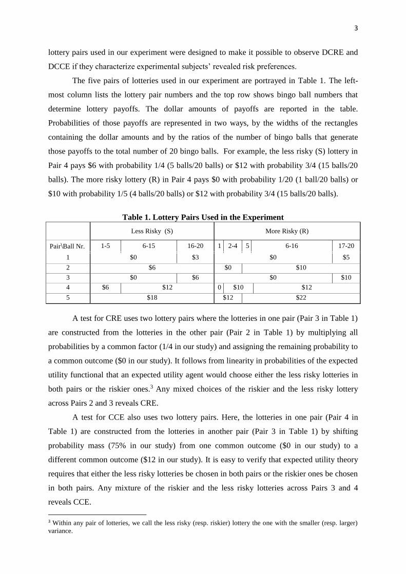
balls numbered 1, 2, …, 20. Lotteries were not shown to participants in the format of Table 1.

They were presented in a format illustrated by the example in Figure 1 which shows one of

the two ways in which the lotteries of Pair 4 were presented to subjects in the experiment.

Ball nr 1 2 3 4 5 6 7 8 9 10 11 12 13 14 15 16 17 18 19 20

Option A

$6

$12

Option B $0

$10

$12

Figure 1. An Example of Presentation of Lotteries

Some subjects would see the Pair 4 lotteries as shown in Figure 1 while others would see

them (randomly) presented with inverted top and bottom positioning and reversed A and B

labeling. (See below for full details on randomized presentation of option pairs.)

13

The experiment was conducted in the laboratory of the Experimental Economics

Center at Georgia State University. Subject instructions are contained in an appendix

available on the journal’s web site. Subjects in groups OTi, i = 1, 2, …, 5, had to perform

simply one choice between the lotteries of Pair i which was played out for real. Subjects in an

OTi treatment were first shown lottery Pair i at the time they made their decision. In treatment

PORnp subjects were first shown a lottery pair at the time they made their decision for that

pair. In all other multiple decision treatments, including PORpi and PORpas, subjects were

shown all five lottery pairs at the beginning of a session, as follows. Each subject was given

an envelope with five (independently) randomly-ordered small sheets of paper. Each of the

five small sheets of paper presented one lottery pair in the format illustrated by Figure 1. Each

subject could display his or her five sheets of paper in any way desired on the table in his or

her private decision carrel.

Subjects entered their decisions in computers in their private decision carrels. In all

treatments, including OT, the top or bottom positioning of the two lotteries in any pair and

their labeling as Option A or Option B were (independently) randomly selected by the

decision software for each individual subject. In all treatments other than OT, the five lottery

pairs were presented to individual subjects by the decision software in independently-drawn

random orders. Each decision screen contained only a single pair of lotteries.

In treatments PAI, PAC, PAC/N, and PAS subjects had to make choices for all five

pairs but here the choice from every pair was played out for real by drawing a ball from a

bingo cage. In treatment PAI the five choices were played out independently at the end of the

experiment whereas in treatments PAC and PAC/N the five choices were played out

correlated at the end of the experiment (i.e., one ball was drawn from the bingo cage which

determined the realized state of the world, hence the payoff of all five choices). In treatment

PAS the chosen lotteries were played immediately after each choice was made (by drawing a

ball from a bingo cage after each decision), and the realized payoff was added to the subject’s

monetary earnings before the next choice was made.

Subjects in treatments PORpi and PORnp had to make choices for all five lottery pairs

and at the end one pair was randomly selected (by drawing a ball from a bingo cage) and the

chosen lottery in that pair was played out for real (by drawing a ball from another bingo cage).

In treatment PORpas subjects had to make choices for all five lottery pairs but the outcome

from each chosen option was realized (by drawing a ball from a bingo cage) before the next

choice option pair was presented to the subject. After all (choices had been made and)

14

outcomes had been realized, one outcome was randomly selected for money payoff (by

drawing a ball from another bingo cage).

In all treatments subjects were permitted to inspect the bingo cage(s) and the balls

before making their decisions. Each ball drawn from a bingo cage was done in the presence of

the subjects and put back in the cage in the presence of the subjects.

5 Tests of classic properties with data from alternative mechanisms

Hypothesis 1 is tested with data from each mechanism as follows. A probit model is used to

estimate the probability of choosing the less risky lottery in Pairs 2 and 3; right-hand variables

include a dummy variable for Pair 3 and subject characteristic variables for Field (of) Study,5

Birth Order, Female, Black, and Older than 21. The question of interest here is whether the

estimated effect of Pair 3 (i.e., the “extra” likelihood of choosing the less risky option in Pair

3) is significantly different from 0; if so, the sign of the estimate will be used to determine

whether our data are characterized by the fanning-in or fanning-out property. We report in the

CRE column of Table 3 whether the estimated effect of Pair 3 is significantly different from

zero with a two-sided test; complete results from the probit estimation for Hypothesis 1 are

reported in appendix Table A.1 (top part). We also report, in the text, one-sided test results

(and one-sided p-values) when there is a familiar one-sided alternative hypothesis.

Table 3. Test Results for Hypotheses 1 - 4

Notes: a. Fan Out; b. Fan In; c. IRRA; d. DRRA; e. IARA

First consider the test of Hypothesis 1 using data from the OT mechanism, reported in

the CRE column and first row of Table 3. We find that OT data do not reject Hypothesis 1,

5 Subjects were asked to report their majors. We have grouped their responses in Science and Engineering,

Business and Economics and Others; the last category will be the base group in our regressions.

Mechanism CRE CCE DCRE DCCE

OT No No No Yese

PORnp No No No No

PORpi No Yesb Yesc No

PORpas Yesa No No No

PAS No Yesb No No

PAI Yesa No No No

PAC/N No Yesb No No

PAC Yesa No Yesd No

15

meaning that the hypothesis of absence of CRE is not rejected. The two-sided p-value on the

Pair 3 dummy variable in the OT column of Table A.1 is 0.127. This test result is reported as

a “No” in the OT row and CRE column of Table 3, which corresponds to the common

practice of reporting a theoretical paradox “has not been observed” in cases when the null

hypothesis of its absence is not rejected.

Data for PORpas, PAI and PAC do reject Hypothesis 1, meaning that the hypothesis of

absence of CRE is rejected. This test result is reported as a “Yes” in the relevant rows of

Table 3. Data for these three mechanisms reject Hypothesis 1 at 5% significance level in favor

of fanning out of indifference curves since the estimated effect of Pair 3 is negative (i.e., the

less risky option is chosen less often in Pair 3 than in Pair 2). The specific pattern (“Fan Out”)

of CRE observed in the data is reported in the footnote to the “Yes” entries in the CRE

column of Table 3; the one-sided p-values are 0.013 (PORpas), 0.035 (PAI) and 0.003 (PAC).

Estimated effects of Pair 3 with data from all other mechanisms are not significantly

different from 0 (two-sided p 0.10), so five out of eight of the multiple-choice-task

mechanisms do not reject Hypothesis 1 (absence of CRE). These findings are reported in the

CRE column of Table 3 as “No”, meaning CRE is not observed.

To be able to compare conclusions we draw from multiple-task treatments with those

for the OT treatment we used the same method of data analysis for all treatments. Since we

do not have within-subjects data for the OT treatment, we began by reporting estimates from

probit regressions that use between-subjects data. But for multiple-task treatments we also

have within-subjects data so we will be able to say more. Counting the number of subjects

who chose the riskier option R in one of the pairs (2 or 3) and the less risky (or safer) option S

in the other, we find the following figures (in percentages): 53%, 38% and 43% in PORnp,

PORpi and PORpas, higher figures of 50% and 45% in PAC/N and PAC, and lower figures of

36% in PAS and 32% in PAI. In testing for statistical significance we need to take into

account that some subjects may be indifferent between the two options within a pair. The null

hypothesis that follows from the indifference argument is that frequencies of safer and riskier

choices (or SR and RS patterns) are similar across Pairs 2 and 3. According to Cochran’s Q

test reported in the last row of the CRE part of Table A.1,6 the null hypothesis of no

systematic violations is rejected by PAC data (p = 0.008) and PORpas data (p = 0.029) and

weakly rejected by PAI data (p = 0.083). These within-subjects test results are consistent with

the between-subjects test results from the probit regression.

6 The Cochran test is the same as the McNemar test since we have only two groupings here.

16

Estimates from probit regression using data for Pairs 3 and 4 of the likelihood of

choosing the less risky option within a pair are used in tests of Hypothesis 2 reported in the

CCE column of Table 3 (and complete results are in the CCE part of appendix Table A.1).

The estimated Pair 4 effect is significant for PORpi data (p = 0.058), PAS data (p = 0.002)

and PAC/N data (p = 0.076); all of these estimates are negative, which is consistent with

indifference curves that Fan In. Estimated Pair 4 effect with data from other mechanisms is

insignificantly different from 0, which is reported as “No” in the CCE column of Table 3. The

p-values for Cochran’s Q test results reported in the CCE part of Table A.1 are: PORpi data

(0.059), PAS data (0.007), and PAC/N data (0.096); p-values for other mechanisms are

greater than 0.1.

Data from the several mechanisms have different implications for testing expected

utility theory. Six of the eight mechanisms produce data that are inconsistent with expected

utility theory because the data either reject Hypothesis 1 or Hypothesis 2 (the entries in Table

3 are “Yes” for presence of CRE or CEE). Furthermore, these mechanisms produce data that

are variously consistent with indifference curves that Fan In, Fan Out, or are parallel.

The test results are less heterogeneous if one looks only at the four mechanisms that

are theoretically incentive compatible for expected utility theory: OT, PORpi, PORnp and

PORpas. Data from three out of four mechanisms do not reject Hypothesis 1, and data for

three out of four do not reject Hypothesis 2, but the mechanism with the one rejection differs

for the two paradoxes.

Results from probit regressions of Hypothesis 3 that use choice data for Pairs 1 and 3

from each payoff mechanism separately are reported in the DCRE column of Table 3 (and

complete results are reported in appendix Table A.2). The estimated Pair 3 effect is

insignificant with data from all mechanisms except PORpi and PAC. Estimation with data

from the PAC mechanism suggests that the likelihood of the less risky option being chosen is

14.5% lower in Pair 3 (p = 0.046), which is consistent with DRRA risk preferences. In

contrast, estimation with data from the PORpi mechanism suggests IRRA risk preferences as

the estimated Pair 3 effect is significant and positive (p = 0.02). Results from the Cochran Q

test reported in the last row of the DCRE part of Table A.2 are generally consistent with the

between-subjects probit analysis.

Results from probit tests of Hypothesis 4 are reported in the DCCE column of Table 3

(and complete results are reported in the DCCE part of appendix Table A.2). Estimated Pair 5

effect (increasing all payoffs by $12) is insignificant (two-sided p-values 0.10) with data

from all mechanisms except OT. Revealed risk preferences with the mechanisms that involve

17

many tasks are consistent with CARA but OT data are consistent with preferences that exhibit

IARA as the sign of the Pair 5 estimate is positive (p = 0.031). For many-task treatments, the

within-subjects analysis is consistent with across-subjects analysis as the Cochran Q test

results reported in the last row of Table A.2 are consistent with the probit test results.

Data from the several mechanisms have divergent implications for testing for CARA

and CRRA within the range of payoffs used in the experiment. Data from three mechanisms

reject either CRRA or CARA whereas data from five mechanisms do not reject either. The

four mechanisms that are incentive compatible for dual theory of expected utility are OT,

PAC, PAC/N and PAS. Two out of these four incentive compatible mechanisms produce data

that are inconsistent with dual theory of expected utility because the data are inconsistent with

either CARA or CRRA (the entries in Table 3 are “Yes” in either the DCRE or DCCE

column).

We have used eight mechanisms to generate risk preference data for five lottery pairs

that have the potential to test for distinguishing properties of different theories of risk

preferences. Out of eight mechanisms, only PORnp seems to be producing data that do not

reject any of the four hypotheses. A central implication from the test results in Table 3 is that

there is strong support for the view that test results for classic paradoxes of decision theory are

dependent on the payoff mechanism that is used to elicit the risk preferences.

6 Revealed risk preferences differ across payoff mechanisms

It has been argued in the literature (e.g., Kahneman and Tversky 1979) that subjects evaluate

each choice independently of the other choice opportunities in an experiment. If this “isolation

hypothesis” were to have robust empirical validity then all mechanisms in our experiment

would elicit the same risk preferences. We ask whether the risk preferences revealed by

subjects differ across treatments that use different payoff mechanisms or whether they are

consistent with isolation of individual choices. The five columns of Table 4 summarize, for

each lottery choice pair i (=1,2,…,5) and each elicitation mechanism, the percentage of

subjects who chose the less risky (or “safer”) lottery in that pair, denoted by Si.

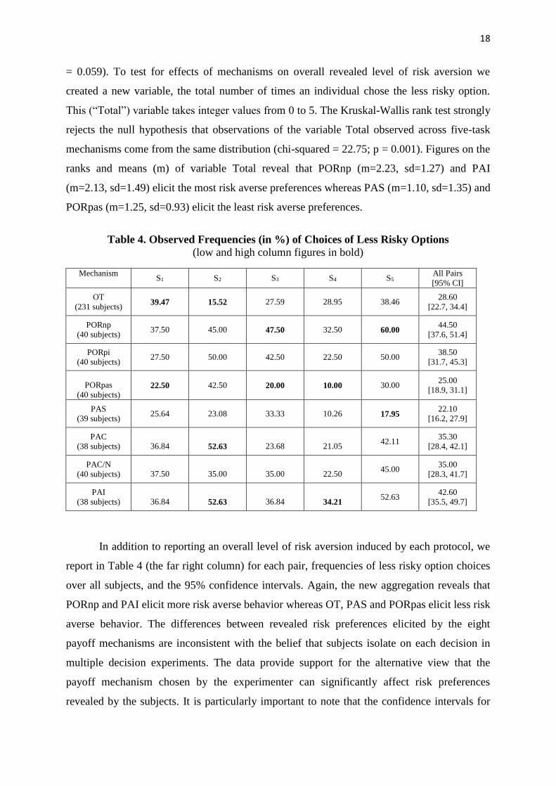
Looking down the Si columns of Table 4 we see that in three out of five columns the

largest figure is more than three times the smallest one: for Pair 2, choices of the less risky

option vary over mechanisms from 15.52% (OT) to 52.63% (PAC and PAI); for Pair 4 these

choices vary from 10.00% (PORpas) to 34.21% (PAI); and for Pair 5, choices of the less risky

option vary from 17.95% (PAS) to 60% (PORnp). The Kruskal-Wallis rank test rejects the

null hypothesis that these frequencies come from the same population (chi-squared = 13.58; p

18

= 0.059). To test for effects of mechanisms on overall revealed level of risk aversion we

created a new variable, the total number of times an individual chose the less risky option.

This (“Total”) variable takes integer values from 0 to 5. The Kruskal-Wallis rank test strongly

rejects the null hypothesis that observations of the variable Total observed across five-task

mechanisms come from the same distribution (chi-squared = 22.75; p = 0.001). Figures on the

ranks and means (m) of variable Total reveal that PORnp (m=2.23, sd=1.27) and PAI

(m=2.13, sd=1.49) elicit the most risk averse preferences whereas PAS (m=1.10, sd=1.35) and

PORpas (m=1.25, sd=0.93) elicit the least risk averse preferences.

Table 4. Observed Frequencies (in %) of Choices of Less Risky Options

(low and high column figures in bold)

Mechanism S1 S2 S3 S4 S5

All Pairs

[95% CI]

OT

(231 subjects) 39.47 15.52 27.59 28.95 38.46

28.60

[22.7, 34.4]

PORnp

(40 subjects) 37.50 45.00 47.50 32.50 60.00

44.50

[37.6, 51.4]

PORpi

(40 subjects) 27.50 50.00 42.50 22.50 50.00

38.50

[31.7, 45.3]

PORpas

(40 subjects) 22.50 42.50 20.00 10.00 30.00

25.00

[18.9, 31.1]

PAS

(39 subjects) 25.64 23.08 33.33 10.26 17.95

22.10

[16.2, 27.9]

PAC

(38 subjects) 36.84 52.63 23.68 21.05 42.11

35.30

[28.4, 42.1]

PAC/N

(40 subjects) 37.50 35.00 35.00 22.50 45.00

35.00

[28.3, 41.7]

PAI

(38 subjects) 36.84 52.63 36.84 34.21 52.63

42.60

[35.5, 49.7]

In addition to reporting an overall level of risk aversion induced by each protocol, we

report in Table 4 (the far right column) for each pair, frequencies of less risky option choices

over all subjects, and the 95% confidence intervals. Again, the new aggregation reveals that

PORnp and PAI elicit more risk averse behavior whereas OT, PAS and PORpas elicit less risk

averse behavior. The differences between revealed risk preferences elicited by the eight

payoff mechanisms are inconsistent with the belief that subjects isolate on each decision in

multiple decision experiments. The data provide support for the alternative view that the

payoff mechanism chosen by the experimenter can significantly affect risk preferences

revealed by the subjects. It is particularly important to note that the confidence intervals for

19

the less risky option choice frequency with PORnp and PAI are disjoint from the confidence

intervals for OT, PORpas and PAS.

The above tests use aggregated data. To retrieve information from data at the

individual level we ran probit regressions with subject clusters to allow for correlated errors

across choice tasks within an individual and with robust standard errors to accommodate

heteroscedasticity. Table 5 reports probit marginal effects of several regressors we consider

on the likelihood of choosing the less risky lottery in a pair. We will discuss results from use

of data for all rounds in (probit) Model 3. The alternatives, Model 1 and Model 2 differ from

Model 3 by exclusion of some of the right-hand variables. We include these alternative

specifications in the table in order to show that our central conclusions about mechanism

effects are robust to alternative specifications of the estimation model.

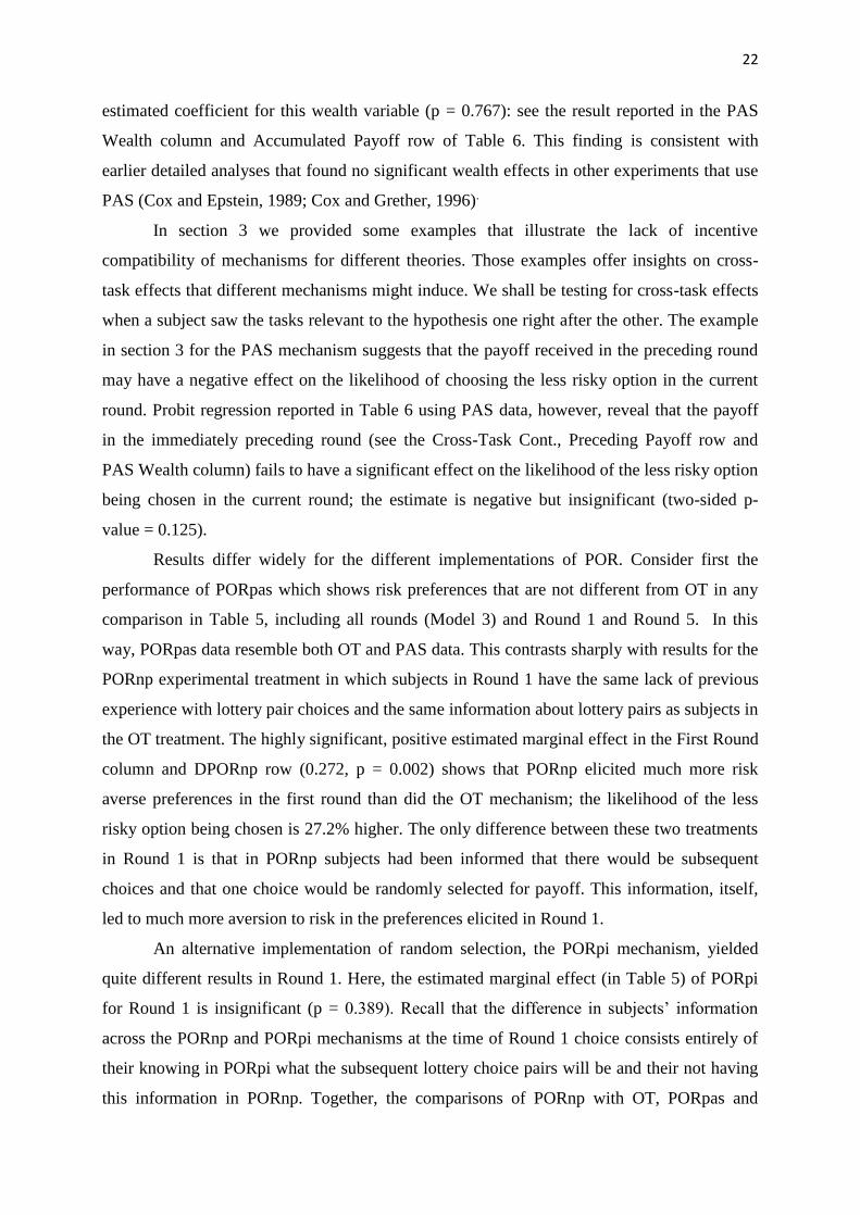
The right hand variables in Model 3 include difference between expected values (EV

Difference) and difference between variances (VAR Difference) of the riskier and safer

lotteries within a pair. The estimated marginal effect for EV Difference is not significant. The

estimated marginal effect for VAR Difference is significantly positive (1.2%, p = 0.002)

which is consistent with aversion to risk: the larger the variance of the riskier option relative

to the less risky one the more likely the less risky option is to be chosen. Some other right-

hand variables are demographic controls for factors commonly associated with between-

subjects differences in risk attitudes. We use dummies for the subjects’ field of study using

three categories: Science and Engineering, Economics and Business, and Other Majors (the

base group). The subject’s Birth Order is significant; subjects who were a younger sibling or

only child were less likely to choose the less risky lottery than an older sibling. Female

subjects were more likely to choose the less risky lottery. Older subjects were less likely to

choose the less risky lottery. Probability of choosing the less risky lottery was not

significantly affected by a subject’s race (Black).

The other variables used in the probit regressions are dummy variables for multiple

decision payoff mechanism treatments. All mechanism treatment dummy variables equal 0 for

OT data. Otherwise, a value equal to 1 for any one of the multiple decision payoff mechanism

dummy variables selects data for that mechanism. The effects of PORnp and PAI mechanisms

on subjects’ choices (in the direction of higher risk aversion) are highly significant at 1%;

other mechanisms with significant coefficients are PORpi (p = 0.040) and PAC (p = 0.080),

and PAC/N (p = 0.051). The signs of the estimated effects of the above multiple decision

mechanisms are all positive, which provides support for the finding that subjects are more

20

likely to choose the less risky option (they appear to be more risk averse) with all multiple

decision payoff mechanisms except PORpas and PAS than they are with the OT protocol.

Table 5 Probit Analysis of Choices of Less Risky Options

All Rounds First Round Last Round

Regressors Model 1 Model 2 Model 3

Pair Characteristics

EV Difference -0.028 -0.028 -0.023 -0.034

(0.431) (0.426) (0.705) (0.585)

VAR Difference 0.012*** 0.012*** 0.007 0.007

(0.002) (0.002) (0.331) (0.357)

Demographics

Science & Engineering 0.037 0.036 -0.008 0.016

(0.267) (0.278) (0.876) (0.759)

Economics & Business 0.022 0.023 0.053 0.002

(0.556) (0.539) (0.331) (0.969)

Birth Order -0.029* -0.029* -0.045** -0.039*

(0.053) (0.053) (0.033) (0.069)

Female 0.094*** 0.096*** 0.038 0.091**

(0.002) (0.002) (0.403) (0.042)

Black 0.041 0.042 0.038 0.059

(0.173) (0.167) (0.388) (0.179)

Older than 21 -0.050 -0.052* -0.005 -0.078*

(0.106) (0.098) (0.915) (0.089)

Treatment Effects

DPORnp 0.171*** 0.143*** 0.149*** 0.272*** 0.182**

(0.001) (0.007) (0.005) (0.002) (0.036)

DPORpi 0.109** 0.104** 0.109** 0.073 0.199**

(0.039) (0.046) (0.040) (0.389) (0.019)

DPORpas -0.036 -0.060 -0.058 0.038 -0.071

(0.435) (0.212) (0.238) (0.655) (0.387)

DPAS -0.068 -0.057 -0.053 -0.050 -0.073

(0.261) (0.340) (0.387) (0.556) (0.392)

DPAC 0.076 0.096* 0.102* 0.099 0.171**

(0.187) (0.095) (0.080) (0.256) (0.048)

DPAC/N 0.073 0.097* 0.104* 0.174** 0.022

(0.183) (0.063) (0.051) (0.041) (0.799)

DPAI 0.152*** 0.175*** 0.183*** 0.169* 0.212**

(0.009) (0.002) (0.002) (0.054) (0.017)

Nr. Of Observations

(Nr. of Subjects)

1,606

(506)

1,606

(506)

1,606

(506)

506

(506)

506

(506)

Log-likelihood -994.0 -991.6 -978.5 -311.8 -304.2

p-values in parentheses: *** p<0.01, ** p<0.05, * p<0.1

The PORpas and PAS mechanisms produce data that clearly differ from data elicited

by other multiple decision mechanisms. We tested for differences between the estimates for

PAS and those for other mechanisms. Using the Model 3 estimates, we find that the estimated

21

effect of PAS is different from the estimated effect of PORnp (p = 0.010) and PAI (p =

0.007), where the figures in parentheses are Bonferroni-adjusted p-values.7

7 Behavioral properties of mechanisms

Inconsistency with the isolation hypothesis makes clear the importance of researching the

behavioral properties of mechanisms. What can account for the discrepancies across

mechanisms in elicited risk preferences? The probit marginal effects reported in section 6

show that subjects were responding to the properties of lotteries within a pair. Our subjects

made choices that reveal risk aversion since increase in the difference between variances of

returns of the riskier and less risky lottery within a pair had a positive effect on the less risky

option being chosen. Other estimates from the demographic variables are consistent with

findings in other studies. The payoff mechanism effects on elicited risk preferences revealed

through treatment estimates (in Table 5) are partly predicted by the incentive incompatibility

examples in section 3 but there is more to the explanation of behavioral properties of

mechanisms.

The probit estimated marginal effects reported in the right-most two columns in Table

5 for data from Round 1 and Round 5 yield further insight into these behavioral properties. It

is important to recall that the choice order of the five lottery pairs is randomly and

independently selected for each subject. Therefore Round 1 and Round 5 choices reported in

Table 5 will each include a random selection of distinct lottery pairs. Hence the dummy

variables for protocols in Round 1 and 5 are picking up choice order effects not lottery pair

effects.

The estimate of the dummy variable coefficient for PAS data shows risk preferences

that are not different from OT in any comparison in Table 5, including all rounds (Model 3)

and Round 1 and Round 5. This is a particularly interesting result because, of all the multi-

decision payoff mechanisms, PAS is the one that has traditionally been suspected of cross-

task contamination (from wealth effects). The way in which PAS might exhibit cross-task

contamination would be if there were a significant wealth effect on risk preferences, in which

case risk preferences elicited in a subsequent round would not be independent of choices and

realized outcomes in earlier rounds. Probit analysis of data from our experiment, that includes

total payoff from lotteries chosen in earlier periods as an explanatory variable for choice

between riskier and less risky options in the current period, finds no significance of the

7 Unadjusted p-values are: 0.002 (PORnp), 0.016 (PORpi), 0.933 (PORpas), 0.001 (PAI), 0.028 (PAC) and 0.018

(PAC/N).

22

estimated coefficient for this wealth variable (p = 0.767): see the result reported in the PAS

Wealth column and Accumulated Payoff row of Table 6. This finding is consistent with

earlier detailed analyses that found no significant wealth effects in other experiments that use

PAS (Cox and Epstein, 1989; Cox and Grether, 1996).

In section 3 we provided some examples that illustrate the lack of incentive

compatibility of mechanisms for different theories. Those examples offer insights on cross-

task effects that different mechanisms might induce. We shall be testing for cross-task effects

when a subject saw the tasks relevant to the hypothesis one right after the other. The example

in section 3 for the PAS mechanism suggests that the payoff received in the preceding round

may have a negative effect on the likelihood of choosing the less risky option in the current

round. Probit regression reported in Table 6 using PAS data, however, reveal that the payoff

in the immediately preceding round (see the Cross-Task Cont., Preceding Payoff row and

PAS Wealth column) fails to have a significant effect on the likelihood of the less risky option

being chosen in the current round; the estimate is negative but insignificant (two-sided p-

value = 0.125).

Results differ widely for the different implementations of POR. Consider first the

performance of PORpas which shows risk preferences that are not different from OT in any

comparison in Table 5, including all rounds (Model 3) and Round 1 and Round 5. In this

way, PORpas data resemble both OT and PAS data. This contrasts sharply with results for the

PORnp experimental treatment in which subjects in Round 1 have the same lack of previous

experience with lottery pair choices and the same information about lottery pairs as subjects in

the OT treatment. The highly significant, positive estimated marginal effect in the First Round

column and DPORnp row (0.272, p = 0.002) shows that PORnp elicited much more risk

averse preferences in the first round than did the OT mechanism; the likelihood of the less

risky option being chosen is 27.2% higher. The only difference between these two treatments

in Round 1 is that in PORnp subjects had been informed that there would be subsequent

choices and that one choice would be randomly selected for payoff. This information, itself,

led to much more aversion to risk in the preferences elicited in Round 1.

An alternative implementation of random selection, the PORpi mechanism, yielded

quite different results in Round 1. Here, the estimated marginal effect (in Table 5) of PORpi

for Round 1 is insignificant (p = 0.389). Recall that the difference in subjects’ information

across the PORnp and PORpi mechanisms at the time of Round 1 choice consists entirely of

their knowing in PORpi what the subsequent lottery choice pairs will be and their not having

this information in PORnp. Together, the comparisons of PORnp with OT, PORpas and

23

PORpi data suggest that the ambiguity of future choice options that subjects faced in PORnp

caused them to behave as if they were more risk averse in Round 1.8

Table 6. Probit Tests of Cross-Task Effects

Mechanism PORnp PORpi PORpas PAS PAI

Regressors CRE CCE CRE CCE CRE CCE “Wealth Wealth Portfolio

Pair Characteristics

EV differences 0.013 -0.223*** 0.186

(0.882) (0.008) (0.127) VAR differences 0.012 0.027*** -0.004

(0.223) (0.002) (0.799)

Cross-Task Cont.

Preceding Payoff

-0.004

(0.498)

-0.007

(0.125)

Preceding Choice 0.266

(0.148)

-0.438**

(0.022)

-0.068

(0.714)

-0.325*

(0.061)

-0.081

(0.442)

-0.026

(0.550)

-0.180

(0.129)

Wealth/ Portfolio

Accumul. Payoff

0.000

(0.990)

0.001

(0.767)

Accumul. S Choices 0.133**

(0.018)

Demographics Yes Yes Yes Yes Yes Yes Yes Yes Yes

Nr. Of Observations 32 30 32 32 28 24 200 195 152

Log-Likelihood -18.76

-14.01

-20.23

-15.90 -10.20

-7.03

-106.9

-88.39

-86.86

Robust p-values in parentheses: *** denotes p<0.01; ** denotes p<0.05; * denotes p<0.1.

The Round 5 results in Table 5 look very different. Here, the estimated marginal

effects for PORnp and PORpi are almost identical but they are significantly different from

zero and from the estimate for PORpas.9 In Round 5 subjects in all POR treatments knew that

this would be their last decision. However, with PORnp and PORpi they were evaluating the

task 5 options within an environment containing a compound lottery reflecting prior-round

option choices whereas with PORpas the environment included a simple lottery over realized

payoffs from prior choices. With PORnp and PORni subjects were significantly more risk

averse in Round 5 than in OT, PAS and PORpas.

Payoff mechanism effects with PORnp and PORpi are reported in other recent papers.

Harrison and Swarthout (2013) study payoff protocol effects on estimated risk attitudes. They

find that RDU estimates with OT (or “1-in-1”) data and PORnp (or “1-in-30”) data are

significantly different whereas the EU estimates are not affected. Cox, et al. (2014) report that

8 See also the discussion in section 10 of biases introduced by use of PORnp in social preferences experiments. 9 Chi2(1)=5.36 and p= 0.021 for estimated effects of PORnp and PORpas being the same and chi2(1)=5.86 and

p= 0.016 for PORpi and PORpas case.

24

the choices elicited by PORpi can be systematically manipulated by inclusion of

asymmetrically dominated choice alternatives, which implies that PORpi does not generally

elicit true risk preferences.

PORnp and PORpi are immune to preceding-payoff cross-task effects because no

lottery payoff is realized before a subsequent choice is made. In order to test for cross-task

effects with PORnp and PORpi, we test for choice order effects on revelation of classical

paradoxes. In this case, as with PAS, we look at adjacent choices but now we focus on the

case in which the pairs involved in a classical paradox were faced by a subject one right after

the other. If there is any cross-task effect of this type one would expect it to be weaker in

PORpi than in PORnp because subjects have already seen all five pairs in advance with the

former implementation of the mechanism. The data support this conjecture. As shown in

Table 3, PORnp does not reveal CRE or CCE when all data are used. In contrast, as shown in

Table 6 (Cross-Task Cont., Preceding Choice row), if we focus only on adjacent choices then

PORnp adjacent data reveal a CCE (p-value = 0.022) but not a CRE (p-value = 0.148). Hence,

PORnp data are characterized by choice order effects as CCE is present in the adjacent

choices but absent otherwise. PORpi adjacent choices data show a weakly significant (p-value

= 0.061) Preceding Choice effect for CCE that is consistent with the all-data result in Table 3

(and the Pair 4(D) effect reported in the PORpi column of Table A.1). With adjacent choice

data for PORpas, we do not find significant cross-task contamination from resolved payoffs

(see the “Preceding Payoff” and “Accumulated Payoff” rows) nor any EU paradoxes (see the

Preceding Choice row). Since CRE is present in the Table 3 test with all data, however, this

inconsistent adjacent-round test result may suggest some possible cross-task contamination.

Comparison of the estimated effects of PAC and PAC/N in Table 5 also yields

behavioral insight into these mechanism effects. Recall that the only difference between these

two mechanisms is the scale of payoffs; experimental treatments with these two mechanisms

are otherwise identical. Subjects in the PAC and PAC/N treatments have the same information

about lotteries in Round 1 and Round 5 as do subjects in the PORpi treatment. Expected

payoffs for PAC are N times as large as for PORpi; they are the same for PAC/N and PORpi.

Choice behavior in PAC follows a similar pattern as in PORpi, with no significant difference

from OT in Round 1 but significantly more risk averse behavior by Round 5. PAC/N follows

the reverse pattern, with significantly more revealed risk aversion than OT in Round 1 but no

difference from OT in Round 5.

The section 3 example of possible portfolio effects from the PAI mechanism shows

how, with uncorrelated lotteries, a portfolio with several riskier options may be preferred to

25

other portfolios even when the agent prefers the less risky lottery to the riskier lottery in

isolation. If so, then we might observe that a current choice of the less risky option has a

positive effect on the likelihood of the less risky option being chosen later.10 Data are

consistent with this conjecture. Probit regression reported in Table 6 (PAI Portfolio column,

Accumulated S choices row) shows a significant positive effect (p = 0.018) of the previous

total number of choices of the less risky option on the likelihood of choosing the less risky

option in the current decision task.

8 Comparisons to previous literature

Several previous studies tested whether POR elicits true preferences and concluded that

serious distortions were not observed. But many of these conclusions are based on

experimental protocols or tests of hypotheses that do not actually support the conclusion of

robust absence of preference distortion by POR.

Camerer (1989) allows subjects to change their choices after the task relevant for

payoff has been randomly selected. Since few people do so, he concludes that POR does not

induce biases. This conclusion, however, implicitly relies on the assumption that decision

makers are “naïve” rather than “resolute” (Machina 1989). If decision makers are resolute

then the other options involved in the POR mechanism could lead to altered preferences and

these altered preferences would still hold after selection of the task relevant for payoff, which

would cause subjects to stick with initially-biased preference revelation.

Starmer and Sugden (1991) and Hey and Lee (2005a)11 test isolation against the

alternative hypothesis that subjects make all choices so as to yield the most preferred

probability distribution of payoffs from the whole experiment (called “full reduction”). Their

tests reject full reduction in favor of the alternative of isolation. But there are many

alternatives to isolation other than full reduction, which is a priori implausible in experiments

in which subjects make a large number of choices and first see a lottery pair when they are

asked to make the choice for that pair (as noted by Hey and Lee 2005a).

Hey and Lee (2005b) report tests that use two “partial reduction” hypotheses that

differ according to whether the current choice task is given the same weight or higher weight

10 This hypothesis is also consistent with a subject who always goes for the safe choice. But if the positive sign

of the estimate of the accumulated number of less risky choices is picking up this effect then we should see a

significant positive estimate in PORpi and PORnp data as well. This is not what we find; the p-values of the

estimate are 0.236 and 0.240 for PORnp and PORpi. 11 In the experiment reported in Hey and Lee (2005a, 2005b), one out of 179 subjects was selected to receive

payment for one out of his or her 30 choices.

26

than all preceding choice tasks when subjects make choices to the yield the most preferred

probability distribution of payoffs. They report that isolation appears to explain the data better

than either form of partial reduction.

Both full and partial reduction are extreme alternatives to the isolation hypothesis.

More plausible alternatives are provided by hypotheses about cross-task contamination, as

supported by our data. This leads us to ask whether cross-task contamination was observed in

previous experiments with POR.

8.1 Cross-task contamination from POR in previous experiments

Starmer and Sugden (1991, pg. 977) reported their two-tailed test for cross-task contamination

with PORpi data was marginally significant (with p-value 0.051).12 They used PORpi and an

“impure” form of OT in which subjects made one incentivized choice following many

hypothetical choices. Beattie and Loomes (1997) used “pure” OT in which the one

incentivized task is not embedded in other decision tasks. They found a significant difference

between responses to PORpi and OT in one of four analyzed choice problems.

8.2 Experiment with impure OT

We conducted a new Impure OT treatment using a payoff protocol similar to the one in

Starmer and Sugden (1991) and Cubitt et al. (1998).13 Seventy-seven subjects participated in

this experiment. Subjects were given envelopes with the five lottery pairs in Table 1 in

random order, as in all of our other treatments except PORnp. The first four decision tasks

have hypothetical payoffs. The fifth task is paid for sure. We analyze data from the fifth task.

In that task, 26 subjects were given option Pair 2, 26 subjects were given Pair 3, and 25

subjects were given Pair 4. Each subject was given four other option pairs in independent

random order.14

Based on our previous findings, we hypothesized that embedding the one paid round

of Impure OT in a multiple decision treatment with four hypothetical payoff decisions would

have an effect on elicited risk preferences similar to that in PORpi and PORnp: that it would

increase the proportion of less risky option choices. This is what we find: the percentage of

less risky choices for the three pairs (2, 3, and 4) is 23.4% with OT and 35% with Impure OT.

12 This result seems to be consistent with our finding of cross-task contamination by POR unless one insists: (a)

on a specific two-tailed test; and (b) that a p-value of 5.1% rather than 5.0% leads to opposite conclusions.

Starmer and Sugden (1991, pg. 977) state (in our view correctly) that “… we cannot claim to have proved, on the

basis of such a test, that the random-lottery incentive system is unbiased.” 13 This experiment was suggested by a referee. 14 We select only CRE and CCE lottery pairs for payoff to stay close to the Starmer and Sugden (1991) design.

27

To compare the elicited risk preferences of Impure OT with those in other treatments, we use

probit regressions of the type reported in Table 5 using only data for the incentivized tasks 2,

3, and 4. These probit estimates, reported in appendix Table A.3, reveal that preferences

elicited by Impure OT are significantly more risk averse than those for OT.

We also looked at whether CRE or CCE is observed with Impure OT data.

We find that in the paid round, the less risky option was chosen by 30.77% (pair 2), 42.31%

(pair 3) and 32% (pair 4) of subjects. Data show neither CRE nor CCE: Fisher’s exact test

reports a p-value of 0.565 for both. Similar to the across-subjects data analysis for OT, we ran

probit regressions using Pair 2, 3, and 4 data and a dummy variable for Pair 3 data (see Table

A.3, CRE and CCE columns). The Pair 3 estimated effect is not significant; the two-sided p-

values are 0.195 (CRE) and 0.268 (CCE). We conclude that neither CRE nor CCE is observed

with our Impure OT data.

9 Implications for choice of mechanism in decision theory experiments

There are two distinct questions that arise in evaluating mechanisms: (a) incentive

compatibility and (b) cross-task contamination. Incentive compatibility is a straightforward

theoretical question. Mechanism cross-task contamination is an empirical question. This leads

us to the topic of spelling out implications of our theoretical and empirical analysis for

experimental methods. We consider three ways of looking at this issue that differ in terms of

the objectives of particular applications of experimental methods.

9.1 All or nothing approach to testing a theory

One coherent approach to testing hypotheses that follow from a particular theoretical model is

to use a payoff mechanism that is incentive compatible for that theory, test the hypotheses,

and state conclusions about the theory. Application of this approach to testing various models

is informed by the content of section 3.

One puzzle in the literature is provided by the widespread use of POR rather than PAS

to test hypotheses for cumulative prospect theory (CPT); see, for examples, papers by

Birnbaum (2004, 2008), Kothiyal et al. (2013), Harrison and Rutström (2009), and Wakker et

al. (2007). It was generally known after results in Holt (1986) that POR places crucial

reliance on the independence axiom that was subsequently explicitly discarded under CPT

(Tversky and Kahneman 1992), which makes POR inappropriate for tests of CPT with

internal theoretical validity. Furthermore, CPT was also specifically developed as a model

28

defined on income, not terminal wealth, hence wealth effects are not relevant. This means that

PAS is a mechanism that should have been used in tests of CPT that would have had internal

theoretical validity.15 Kachelmeir and Shehata (1992) did use PAS to pay their subjects in

tests of CPT, however their data are confounded by use of the Becker et al. (1964) mechanism

to elicit certainty equivalents, which also requires the independence axiom for its incentive

compatibility (Karni and Safra 1987).

9.2 Nuanced approach to testing a theory

There are issues distinct from incentive compatibility that arise in a nuanced approach to

testing theory in which the researcher is concerned about the source of consistency or

inconsistency with hypotheses. A good example is provided by the tests for CCE reported in

sections 5 and 8. PORpi is incentive compatible for expected utility theory (EU), hence the

significant inconsistency with CCE with data from that mechanism has internal theoretical

validity. But PORnp, PORpas, OT, and Impure OT are also incentive compatible for EU and

data from our treatments with those mechanisms do not exhibit CCE. The difference in test

results comes from the different behavioral properties of the payoff mechanisms, all of which

are theoretically incentive compatible for EU. A nuanced approach to testing a theoretical

hypothesis will try to discriminate between inconsistencies with theory that are specific to one

incentive compatible payoff mechanism and patterns of inconsistency that are robust to other

incentive compatible mechanisms. The clear implication for experimental methods is to avoid

drawing conclusions about fundamental properties such as CCE by running an experiment

using only one of the incentive compatible mechanisms.

9.3 Discriminating between theories

Research on decisions under risk includes experiments designed to discriminate between

alternative theories; see, for examples, Camerer (1989) and Hey and Orme (1994). Design of

experiments of this type encounters an especially difficult issue of incentive compatibility

because a payoff mechanism that is incentive compatible for one of the theoretical models

being compared is typically not incentive compatible for one or more of the other theoretical

models if subjects make multiple decisions. This problem is present in the experiments

reported by Camerer (1989) and Hey and Orme (1994) that asked subjects to make multiple

15 The literature on CPT experiments also includes many papers in which subjects were not paid salient rewards

for any decision (e.g, Abdellaoui et al. 2007, Birnbaum and Chavez 1997, Bleichrodt, et al. 2001, Lopes and

Oden 1999, and Gonzalez and Wu 1999). Previous research shows that hypothetical payoffs can lead to opposite

conclusions than monetary payoffs in some experiments on decisions under risk (e.g., Cox and Grether, 1996).

29

decisions and paid them using some version of POR. Such experiments could be conducted

using OT, as that mechanism is incentive compatible for all theories. Experiments comparing

cumulative prospect theory with the expected utility of income model would have theoretical

validity if they used PAS because both models are defined on income, not terminal wealth.

Experiments comparing linear cumulative prospect theory with dual theory of expected utility

using cosigned lotteries would have theoretical validity if they used PAC, PAC/N or PAS.

It is possible to discriminate between alternative theories using data from mechanisms

other than OT. The problem with many studies that test non-EUT theories with POR data is

that they interpret the observed choices of, say, A1 and B2 and A3 as revealing that the subject

ranks option A1 weakly higher than the alternative option B1, and B2 weakly higher than A2,

and A3 weakly higher than B3; this is of course not correct unless the maintained theory is EU

(see section 3). But data do reveal subjects’ preferences over options conditional on the

incentives provided by the payoff mechanism. Consider, for example, PORpi and three

decision tasks of choosing between options Ai and Bi for i =1,2,3. Regardless of which theory

the researcher is applying, observations such as choice of A1 (rather than B1) and B2 (rather

than A2) and A3 (rather than B3) with PORpi payoffs reveal that the subject ranks lottery R =

(A1,1/3;B2,1/3;A3,1/3) weakly higher than any other feasible lottery, including lotteries P =

(B1,1/3;B2,1/3;A3,1/3) and Q = (A1,1/3;B2,1/3;B3,1/3). However, the observed choices do not

tell us how the subject ranks lotteries P and Q, nor how she ranks Ai and Bi in the absence of

assumption of the independence axiom. Hence, it is logically coherent to conclude from the

observed choices that a maintained theory’s functional evaluated for lottery R has higher

value than that theory’s functional evaluated for P (or Q, or another feasible compound

lottery). One can use this information to make inferences about risk preferences of the subject,

given the theory, by using the composition of the theory’s functional and the functional form

of the payoff mechanism.

10 More implications for experimental methods

Issues raised in studying the theoretical and behavioral properties of payoff mechanisms have

broad implications for experimental methods. We here consider a few illustrative examples.

10.1 Examples of experiments on ambiguity

Empirical failure of isolation is clearly a problem for the growing literature on experiments

with theories of decision under uncertainty and ambiguity that do not include the

independence axiom. These experiments typically involve many decisions and use PORnp as

30

the payoff mechanism (e.g., Abdellaoui et al. 2011, Charness et al. 2013). This means that the

data may reflect confounds and biases from two sources: incentive incompatibility and

behavioral cross-task contamination. Payoff mechanism incentive incompatibility is a central

logical question that has simply been ignored in this literature. In addition, there are issues of

possible cross-task contamination that arise in ambiguity experiments that are similar to those

found in data from our risk experiments. Experiments on ambiguity could use OT to avoid

confounds in the data from payoff mechanism effects. Or they could analyze data with an

approach analogous to the one described for risk theories in the last paragraph of section 9.

10.2 Examples of experiments on social preferences

Many experiments on social preferences involve decisions under risk or uncertainty. For

example if a first mover in an investment game experiment (Berg et al. 1995) sends money to

the second mover, the first mover’s monetary payoff in the experiment is risky (or uncertain)

because it depends on the subsequent return decision of the second mover. Many social

preferences experiments involve between-subjects designs with one shot games (e.g., Berg, et

al. 1995), hence are using OT. But many other experiments include multiple decisions under

risk (or uncertainty) and use some mechanism for paying the subjects. The most commonly

used mechanism for multiple-decision social preferences experiments is PAS (e.g. Bohnet et

al. 2008, Charness and Haruvy 2002, Fehr and Gachter 2000, 2002, and Fehr and Schmidt

2004), which has internal theoretical validity for income models of decision under risk.

Some papers, however, report experiments with role reversal (hence two decisions)

and use PAI (e.g., Burks et al. 2003, Chaudhuri and Gangadharan 2007), which has internal

theoretical validity only for expected value theory; for risk averse subjects, these experiments

involve portfolio incentives that confound drawing conclusions from the data. We believe use

of PAI should be avoided unless the researcher is willing to model its portfolio incentives in

econometric analysis of the data. PORpas or PORpi would be better choices if the maintained

theory is consistent with reduction and independence. PAS would be a good choice if the

maintained theory is defined on income or the researcher checks for possible wealth effects on

second round choices.

Other researchers (e.g, Charness and Rabin 2002) use hybrids of the PAI and PORnp

mechanisms in which some number of decisions larger than one are randomly selected for

payoffs that are determined by PAI. Such hybrid mechanisms may contain both the portfolio

incentives of PAI and the behavioral cross-task contamination of PORnp, and should be

avoided. Use of PAS should be seriously considered as a better mechanism for such

31

experiments. If a researcher is concerned about possible wealth effects from PAS (even if they

are undocumented), or its cost, then serious consideration should be given to use of PORpas

(unless the maintained theory is inconsistent with the independence axiom).

Experiments intended to “identify” trust and reciprocity or “decompose” trust and

trustworthiness inherently involve decisions in more than one game or decision task. Trust can

be identified in a between-subjects design with OT using the investment and triple dictator

games (Cox 2004). Within-subjects designs with PAI for multiple tasks, such as a risk game

and investment game and triple dictator game (Etang et al. 2011), cannot identify trust

because responses are confounded by portfolio incentives. Use of PAI in such experiments

should be avoided in favor of between-subjects designs and OT.

Ashraf et al. (2006) use a within-subjects design, with two tasks including a trust game

and risk game, and use PORnp (where a subject makes one decision in each treatment). The

within-subjects design with PORnp has internal theoretical validity for expected utility theory

but there can be cross-task contamination that biases data with this type of protocol, as has

been reported in papers that tested for it. For example, Cox (2009) reports an experiment in

which data show that informing subjects there will be another unspecified decision task

following a dictator game significantly shifts their behavior towards greater generosity even in

an experiment in which there is anonymity (because of double-blind payoffs) and random

selection of one task for payoff. With this implementation of the PORnp mechanism, subjects

do not isolate their play in a dictator game from the other decision task in the experiment.

Cox et al (2008) report three experiments with different designs for the moonlighting game

and dictator control games. Experiment 2 has a within-subjects design for the moonlighting

game and dictator control games and uses the PORnp mechanism to pay subjects. Experiment

3 has a between-subjects design for the moonlighting game and dictator control game and

pays subjects with OT. Data show that subjects are more trusting and fearful in Experiment 2

than in Experiment 3. With this implementation of the PORnp mechanism, subjects do not

isolate their play in the moonlighting game from their play in the dictator game. Both of these

papers (Cox 2009 and Cox et al. 2008) test for and find cross-task contamination (between

treatments) from the PORnp mechanism in the context of social preferences experiments. A

clear implication is that a researcher running this type of multiple-treatment experiment

should use a between-subjects design and OT, not a within-subjects design and PORnp.

32

10.3 Examples of experiments on public goods and voting

Experiments on voluntary provision of public goods (VCM) or on voting often include

multiple rounds and use PAS (e.g., Isaac and Walker 1988; Montero et al. 2008). As is

recognized in the literature, such designs can involve repeated game incentives. Use of PAS is

a good choice if the data analysis assumes that subjects are playing a repeated game or if

repeated game effects inherent in multiple rounds is effectively controlled.

Goeree et al. (2002) report an experiment in which subjects make 10 VCM decisions

(involving different internal and external marginal return rates) without feedback. PORnp was

used for payoff from the VCM rounds. Subjects were told in advance that the VCM treatment

(“experiment”) would be followed by another treatment (“experiment”) that would pay money

but were not given any information about the nature of the second treatment. They were told

that their earnings from the VCM treatment would be computed during the second treatment

and payoffs from both treatments would be paid at the end. Bosman et al. (2013) report an

experiment on voting in which subjects play the stage game with observed actions 50 times.

Subjects were told that 10 rounds would be randomly selected at the end of experiment and

payoffs from those 10 decisions would all be paid. The former protocol embeds PORnp (for

VCM) within PAI (for the two treatments), whereas the latter embeds PORpi (for the stage

game) within PAI (10 rounds not 1 round for random selection). Hence they can introduce

confounds from interaction of the cross-task contamination problems of POR and PAI

mechanisms. Embedding POR within PAI should be avoided. The use of OT would avoid

confounds. If subject task experience is believed to be important and the interest is on the

stage game behavior then Impure OT is a possibility. Alternatively, PAS could be used with

only the known last period used in data analysis or the behavior of subjects in a repeated game

analyzed using data from all rounds and properly accounting for interim payoffs.

10.4 Examples of experiments on bargaining

Bolton (1991) reports an experiment with ten-round alternating offer bargaining games in

which outcomes are announced each round but two rounds are randomly selected for payoff at

the end of the experiment. Random selection of two rounds creates an incentive for portfolio

decisions across rounds. A better procedure would be to use PAS, because it is incentive

compatible for income models, and modeling wealth effects (required in repeated games

analysis) is less challenging than modeling cross-task contamination and portfolio effects.

Rapoport et al. (1996) experiment with ultimatum games in which the size of the pie is

33

known to the proposer but a random variable with a uniform distribution for the responder.

Subjects make multiple decisions as both proposers and responders. An individual subject’s

payoff was determined in the following way. At the end of the experiment, three trials were

chosen randomly including two where the subject was assigned the role of sender and one

where she played the role of receiver. The subject was paid the outcome on these three trials.

This payoff protocol embeds PORnp within PAI, which can produce data confounded by the

interaction of cross-task contamination by both mechanisms. If subject task experience and

role reversal are believed to be important then Impure OT could be considered for use instead

of the composition of PORnp and PAI.

Recent data show effects from selection of payoff mechanism in bargaining

experiments even when both mechanisms are incentive compatible. Sadiraj and Sun (2012)

conduct an experiment on bargaining with alternating offers on gain and loss domains using

POR and Impure OT payoff protocols. They report that Impure OT induces more efficient

bargaining behavior than POR and that the effect is more pronounced when subjects bargain

over the distribution of gains than the shares of losses.

11 Summary

If it were true that subjects isolate each individual decision in multiple decision experiments

then choice of payoff mechanism would be an unimportant detail. But it is not generally true;

therefore choice of payoff mechanism has central importance for the validity of conclusions

that can be drawn from data. We have evaluated mechanisms on the basis of two criteria: (a)

incentive compatibility and (b) cross-task contamination.

Use of a mechanism that is not incentive compatible with a model to experimentally

generate data to test that model is not logically coherent. Indeed, researchers using this

approach have been dubbed “bipolar behaviorists” by Harrison and Swarthout (2013).

Sections 3 and 9 present what we believe to be the current state of knowledge about incentive

compatibility of mechanisms for prominent theories of decision under risk. Section 10

presents a few examples that illustrate how these results have implications for a much broader

range of experimental research than experiments on decision theory. The paper contains many

explicit and implicit critiques of experimental methods. It also contains many positive

recommendations about choice of mechanism for a variety of specific contexts. But there is

no known “ideal mechanism” that will solve all the problems we describe.

Use of a mechanism that is incentive compatible but has bad behavioral properties,

such as demonstrable cross-task contamination, may be logically coherent but would not

34

appear to represent sound empirical methods. In this respect, the widespread use of the

PORnp mechanism is particularly hard to defend. It has demonstrable cross-task

contamination (see section 7) and has frequently been used in contexts in which it is known

not to be incentive compatible (see sections 9 and 10).

Many studies could solve the incentive compatibility problem by use of the OT

mechanism but this would entail high cost of subject payoffs that in some designs would be

prohibitive. One approach that we describe in section 9.3 needs more formal theoretical

development and econometric application. We describe it briefly here again. Even in the

absence of the independence axiom, one can use the composition of a theory’s utility

functional and the functional form of a pay one randomly mechanism (such as PORpi or

PORpas) to test propositions following from theory. The problem at the heart of numerous

misapplications of such mechanisms is a strategy for data analysis based on the assumption

that choice of, say, Ak rather than Bk, in the context of multiple other choices, reveals a

truthful pairwise preference for Ak even though the theory being tested implies that

preferences may not be truthfully revealed with the chosen mechanism.

35

References

Abdellaoui, M., Baillon, A., Placido, L. & Wakker, P. P. (2011). The rich domain of

uncertainty: source functions and their experimental implementation. American

Economic Review, 101, 695-723.

Abdellaoui, M., Barrios, C. & Wakker, P.P. (2007). Reconciling introspective utility with

revealed preference: experimental arguments based on prospect theory. Journal

of Econometrics, 138, 356-378.

Allais, M. (1953). Le comportement de l’homme rationnel devant le risque: critique des

postulats et axiomes de l’école américaine. Econometrica, 21, 503-546.

Ashraf, N., Bohnet, I., & Piankov, N. (2006). Decomposing trust and trustworthiness.

Experimental Economics, Special Issue on Behavioral Economics, 9(3), 193-208.

Azrieli, Y., Chambers, C. P. & Healy, P. J. (2013). Incentives in experiments: a

theoretical analysis. Working Paper, Ohio State University.

Baltussen, G., Post, G. T., van den Assen, M. J., & Wakker, P. P. (2012). Random incentive

systems in a dynamic choice environment. Experimental Economics, 15, 418-443.

Beattie, J. & Loomes, G. (1997). The Impact of incentives upon risky choice experiments.

Journal of Risk and Uncertainty, 14, 149-62.

Becker, G. M, DeGroot, M. H., & Marschak, J. (1964). Measuring utility by a single-response

sequential method. Behavioral Science, 9, 226-232.

Berg, J., Dickhaut, J., & McCabe, K. (1995). Trust, reciprocity, and social history. Games

and Economic Behavior, 10, 122–142.

Birnbaum, M. H. (2004). Tests of rank-dependent utility and cumulative prospect

theory in gambles represented by natural frequencies: effects of format, event framing,

and branch splitting. Organizational Behavior and Human Decision Processes, 95,

40–65.

Birnbaum, M. H. (2008). New tests of cumulative prospect theory and the priority

heuristic:probability-outcome tradeoff with branch splitting. Judgment and

Decision Making, 3(4), 304–316

Birnbaum, M. H. & Chavez, A. (1997). Tests of theories of decision making: violations

of branch independence and distribution independence. Organizational Behavior

and Human Decision Processes, 71(2), 161–194.

36

Bleichrodt, H., Pinto, J. L. & Wakker, P. P. (2001). Making descriptive use of prospect

theory to improve the prescriptive use of expected utility. Management Science

47(11), 1498-1514.

Bohnet, I., Greig, F., Herrmann, B. & Zeckhauser, R. (2008). Betrayal aversion. American

Economic Review, 98(1), 294-310.

Bolton GE (1991) A comparative model of bargaining: theory and evidence. American

Economic Review, 81(5), 1096–1136.

Bosman, R., Maier, P., Sadiraj, V. & Van Winden, F. (2013). Let me vote! An experimental

study of vote rotation in committees. Journal of Economic Behavior and

Organization, 96, 32-47.

Burks, S. V., Carpenter, J. P. & Verhoogen, E. (2003). Playing both roles in the trust

game. Journal of Economic Behavior and Organization, 51, 195-216.

Camerer, C. F. (1989). An experimental test of several generalized utility theories. Journal of

Risk and Uncertainty, 2, 61-104.

Charness, G. & Haruvy, E. (2002). Altruism, equity, and reciprocity in a gift-exchange

experiment: an encompassing approach. Games and Economic Behavior, 40(2),

203-231.

Charness, G., Karni, E. & Levin, D. (2013). Ambiguity attitudes and social interactions: an

experimental investigation. Journal of Risk and Uncertainty, published online 25

January 2013.

Charness G, & Rabin M (2002). Understanding social preferences with simple tests.

Quarterly Journal of Economics, 117(3), 817–869.

Chaudhuri, A. & Gangadharan, L. (2007). An experimental analysis of trust and

trustworthiness. Southern Economic Journal, 73, 959-985.

Cox, J. C. (2004). How to identify trust and reciprocity. Games and Economic Behavior,

46(2), 260-281.

Cox, J. C. (2009). Trust and reciprocity: implications of game triads and social contexts.

New Zealand Economic Papers. Special Issue: Laboratory Experiments in Economics,

Finance and Political Science, 43(2), 89 – 104.

Cox, J. C. & Epstein, S. (1989). Preference reversals without the independence axiom.

American Economic Review, 79(3), 408-426.

Cox, J. C. & Grether, D. A. (1996). The preference reversal phenomenon: response

mode, markets, and incentives. Economic Theory, 7(3), 381-405.

37

Cox, J. C., Sadiraj, K. & Sadiraj, V. (2008). Implications of trust, fear, and reciprocity

for modeling economic behavior. Experimental Economics, 11, 1-24.

Cox, J. C., Sadiraj, K. & Schmidt, U. (2014). Asymmetrically dominated choice problems, the

isolation hypothesis and random incentive mechanisms. PLOS ONE, March 20, 2014

(in press).

Cubitt, R. P., Starmer, C. & Sugden, R. (1998). On the validity of the random lottery

incentive system. Experimental Economics, 1, 115-131.

Cubitt, R. P., Starmer, C., & Sugden, R. (2001). Discovered preferences and the experimental

evidence of violations of expected utility theory. Journal of Economic Methodology, 8,

385-414.

Etang A., Fielding D., & Knowles, S. (2011). Does trust extend beyond the village?

Experimental trust and social distance in Cameroon. Experimental Economics, 14(1),

15–35.

Fehr, E. & Gächter, S. (2000). Cooperation and punishment in public goods experiments.

American Economic Review, 90(4), 980-994.

Fehr, E. & Gächter, S. (2002). Altruistic punishment in humans. Nature, 415, 137-140.

Fehr, E. & Schmidt, K. M. (2004). Fairness and incentives in a multi-task principal-agent

model. Scandinavian Journal of Economics, 106(3), 453-474.

Goeree, J. K., Holt, C. A., & Laury, S. K. (2002). Private costs and public benefits:

unraveling the effects of altruism and noisy behavior. Journal of Public

Economics, 83(2), 255-276.

Gonzalez, R. & Wu, G. (1999). On the shape of the probability weighting function.

Cognitive Psychology, 38, 129–166

Harrison, G.W. & Rutström, E. E. (2009). Expected utility and prospect theory: one

wedding and a decent funeral. Experimental Economics, 12, 133-158.

Harrison, G.W. & Swarthout, J. T. (2013). Experimental payment protocols and the

bipolar behaviorist. Working paper, Center for the Economic Analysis of Risk,

Georgia State University.

Hey, J. D. & Lee, J. (2005a). Do subjects separate (or are they sophisticated? Experimental

Economics, 8, 233-265.

Hey, J. D. & Lee, J. (2005b). Do subjects remember the past? Applied Economics, 37, 9-18.

Hey, J. D. & Orme, C. (1994). Investigating generalizations of expected utility theory

using experimental data. Econometrica, 62, 1291-1326.

38

Holt, C. A. (1986). Preference reversals and the independence axiom. American Economic

Review, 76, 508-515.

Holt, C. A. & Laury, S. K. (2002). Risk aversion and incentive effects. American

Economic Review, 92, 1644-1655.

Isaac R.M., & Walker J.M. (1988). Group size effects in public goods provision: the

voluntary contributions mechanism. Quarterly Journal of Economics, 103(1), 179-

199.

Kachelmeier, S. J. & Shehata, M. (1992). Examining risk preferences under high

monetary incentives: experimental evidence from the people's republic of china.

American Economic Review, 82(5), 1120-1141.

Kahneman, D. & Tversky, A. (1979). Prospect theory: an analysis of decision under risk.

Econometrica, 47, 263-291.

Karni, E. & Safra, Z. (1987). “Preference reversal” and the observability of preferences by

experimental methods. Econometrica, 55(3), 675-685.

Kothiyal, A., Spinu,V. & Wakker, P. P. (2013). An experimental test of prospect theory for

predicting choice under ambiguity. Journal of Risk and Uncertainty, forthcoming.

Lopes, L. L. & Oden, G. C. (1999). The role of aspiration level in risky choice: a

comparison of cumulative prospect theory and SPA theory. Journal of

Mathematical Psychology 43, 286-313.

Machina, M. J. (1982). “Expected utility” analysis without the independence axiom.

Econometrica, 50, 277-323.

Machina, M. J. (1989). Dynamic consistency and non-expected utility models of choice

under uncertainty. Journal of Economic Literature, 27(4), 1622-1668.

Montero, M., Sefton, M, & Zhang, P. (2008). Enlargement and the balance of power: an

experimental study. Social Choice and Welfare, 30, 69-87.

Neilson, W. S. (1992). A mixed fan hypothesis and its implications for behavior toward

risk. Journal of Economic Behavior and Organization, 19, 197-211.

Sadiraj, V. & Sun, J. (2012). Efficiency in bargaining games with alternating offers.

Economics Bulletin, 32 (3), 2366-2374.

Schmidt, U., & Zank, H. (2009). A simple model of cumulative prospect theory.

Journal of Mathematical Economics, 45, 308–319.

39

Starmer, C., & Sugden, R. (1991). Does the random lottery incentive system elicit true

preferences? an experimental investigation. American Economic Review, 81(4), 971–

978.

Tversky, A., & Kahneman, D. (1992). Advances in prospect theory: cumulative

representation of uncertainty. Journal of Risk and Uncertainty, 5, 297-323.

Wakker, P. P., Köbberling, V., & Schwieren, C. (2007). Prospect-theory’s diminishing

sensitivity versus economics’ intrinsic utility of money: how the introduction of the

euro can be used to disentangle the two empirically. Theory and Decision, 63(3),

205-231.

Yaari, M. E. (1987). The dual theory of choice under risk. Econometrica, 55, 95-115.

40

Appendix Tables

Table A.1. Tests of EU Paradoxes

Mechanisms OT

PORnp PORpi PORpas PAS PAC PAC/N PAI

CRE

Across subjects

Estimated Marginal

Effect of Pair 3 (D) 0.120 0.022 -0.082 -0.239** 0.102 -0.314*** 0.004 -0.195*

(0.127) (0.858) (0.429) (0.025) (0.314) (0.006) (0.972) (0.071)

Demographics Yes Yes Yes Yes Yes Yes Yes Yes

Nr of subjects 116 40 40 40 39 38 40 38

Within subjects

(%) “Violations“

Obs. {SR, RS}

52.50

{10, 11}

37.50

{9, 6}

42.50

{13, 4}

35.90

{5, 9}

44.74

{14, 3}

50.00

{10, 10}

31.58

{9, 3}

Cochran’s chi2 (1)

(Pr. > chi2)

{Exact p}

0.048

(0.827)

{1.000}

0.600

(0.439)

{0.607}

4.76**

(0.029)

{0.049}

1.14

(0.285)

{0.424}

7.12***

(0.008)

{0.013}

0.00

(1.000)

{1.000}

3.00*

(0.083)

{0.146}

CCE

Across subjects

Estimated Marginal

Effect of Pair 4 (D) 0.016 -0.156 -0.207* -0.101 -0.231*** -0.023 -0.143* -0.024

(0.865) (0.237) (0.058) (0.189) (0.002) (0.811) (0.076) (0.834)

Demographics Yes Yes Yes Yes Yes Yes Yes Yes

Nr of subjects 96 40 40 40 39 38 40 38

Within subjects

(%) “Violations“

Obs. {SR, RS}

60.00

{15, 9}

45.00

{13, 5}

25.00

{7, 3}

28.21

{10, 1}

34.21

{7, 6}

22.50

{7, 2}

39.47

{8, 7}

Cochran’s chi2 (1)

(Pr. > chi2)

{Exact p}

1.50

(0.221)

{0.308}

3.56*

(0.059)

{0.096}

1.6

(0.206)

{0.344}

7.36***

(0.007)

{0.012}

0.08

(0.782)

{1.000}

2.78

(0.096)

{0.180}

0.067

(0.796)

{1.000}

p-values in parentheses: *** if p<0.01; ** if p<0.05; * if p<0.1

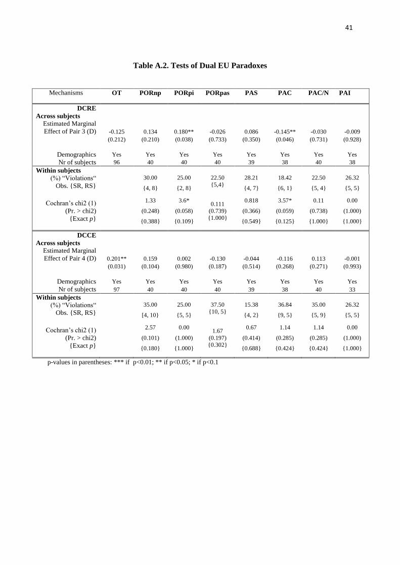
41

Table A.2. Tests of Dual EU Paradoxes

Mechanisms OT PORnp PORpi PORpas PAS PAC PAC/N PAI

DCRE

Across subjects

Estimated Marginal

Effect of Pair 3 (D) -0.125 0.134 0.180** -0.026 0.086 -0.145** -0.030 -0.009

(0.212) (0.210) (0.038) (0.733) (0.350) (0.046) (0.731) (0.928)

Demographics Yes Yes Yes Yes Yes Yes Yes Yes

Nr of subjects 96 40 40 40 39 38 40 38

Within subjects

(%) “Violations“

Obs. {SR, RS}

30.00

{4, 8}

25.00

{2, 8}

22.50

{5,4}

28.21

{4, 7}

18.42

{6, 1}

22.50

{5, 4}

26.32

{5, 5}

Cochran’s chi2 (1)

(Pr. > chi2)

{Exact p}

1.33

(0.248)

{0.388}

3.6*

(0.058)

{0.109}

0.111

(0.739)

{1.000}

0.818

(0.366)

{0.549}

3.57*

(0.059)

{0.125}

0.11

(0.738)

{1.000}

0.00

(1.000)

{1.000}

DCCE

Across subjects

Estimated Marginal

Effect of Pair 4 (D) 0.201** 0.159 0.002 -0.130 -0.044 -0.116 0.113 -0.001

(0.031) (0.104) (0.980) (0.187) (0.514) (0.268) (0.271) (0.993)

Demographics Yes Yes Yes Yes Yes Yes Yes Yes

Nr of subjects 97 40 40 40 39 38 40 33

Within subjects

(%) “Violations“

Obs. {SR, RS}

35.00

[4, 10}

25.00

{5, 5}

37.50

{10, 5}

15.38

{4, 2}

36.84

{9, 5}

35.00

{5, 9}

26.32

{5, 5}

Cochran’s chi2 (1)

(Pr. > chi2)

{Exact p}

2.57

(0.101)

{0.180}

0.00

(1.000)

{1.000}

1.67

(0.197)

{0.302}

0.67

(0.414)

{0.688}

1.14

(0.285)

{0.424}

1.14

(0.285)

{0.424}

0.00

(1.000)

{1.000}

p-values in parentheses: *** if p<0.01; ** if p<0.05; * if p<0.1

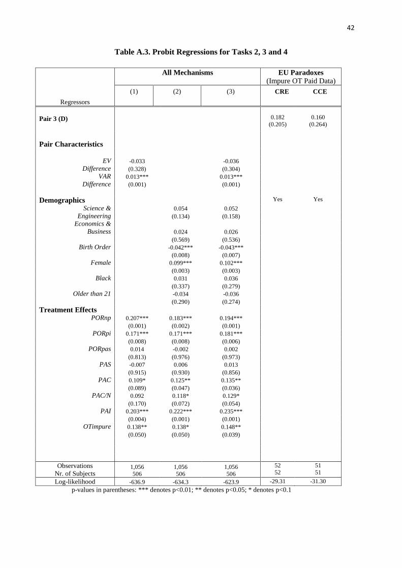
42

Table A.3. Probit Regressions for Tasks 2, 3 and 4

Regressors

All Mechanisms EU Paradoxes

(Impure OT Paid Data)

(1) (2) (3) CRE CCE

Pair 3 (D)

0.182

(0.205)

0.160

(0.264)

Pair Characteristics

EV -0.033 -0.036

Difference (0.328) (0.304)

VAR 0.013*** 0.013***

Difference (0.001) (0.001)

Demographics Yes Yes

Science & 0.054 0.052

Engineering (0.134) (0.158)

Economics &

Business 0.024 0.026

(0.569) (0.536)

Birth Order -0.042*** -0.043***

(0.008) (0.007)

Female 0.099*** 0.102***

(0.003) (0.003)

Black 0.031 0.036

(0.337) (0.279)

Older than 21 -0.034 -0.036

(0.290) (0.274)

Treatment Effects

PORnp 0.207*** 0.183*** 0.194***

(0.001) (0.002) (0.001)

PORpi 0.171*** 0.171*** 0.181***

(0.008) (0.008) (0.006)

PORpas 0.014 -0.002 0.002

(0.813) (0.976) (0.973)

PAS -0.007 0.006 0.013

(0.915) (0.930) (0.856)

PAC 0.109* 0.125** 0.135**

(0.089) (0.047) (0.036)

PAC/N 0.092 0.118* 0.129*

(0.170) (0.072) (0.054)

PAI 0.203*** 0.222*** 0.235***

(0.004) (0.001) (0.001)

OTimpure 0.138** 0.138* 0.148**

(0.050) (0.050) (0.039)

Observations

Nr. of Subjects 1,056

506

1,056

506

1,056

506

52

52

51

51

Log-likelihood -636.9 -634.3 -623.9 -29.31 -31.30

p-values in parentheses: *** denotes p<0.01; ** denotes p<0.05; * denotes p<0.1