Embed Size (px)
Citation preview

Politecnico di Milano
School of Industrial and Information Engineering
Master of Science in Space Engineering
Department of Aerospace Science and Technology
Parafoil Control Authority for Landingon Titan
Candidate:Luca Ermolli, 862458
Politecnico di Milano
Supervisor:Prof. Michele LavagnaPolitecnico di Milano
Mentor:Dr. Marco QuadrelliJet Propulsion Laboratory, California Institute of Technology
Academic Year 2016/2017

This research was carried out at Jet Propulsion Laboratory, California Institute of Technology,during an internship under the JVSRP (JPL Visiting Student Research Program).

Executive Summary
The objective of this work is the development of physics models and simulations techniques forparafoil flight dynamics in Titan environment. This is a preliminary study which has the aimof understanding if advantages given by parafoils high maneuverability can be exploited in thedevelopment of planetary vehicles.
The derivation of a dynamical model describing the parafoil and its response to the presenceof disturbances (drift and gust wind) are important in this problem. Moreover, the applicationof parafoils to space environment implies deep studies on which forces and effects usually presentin common parachutes modeling have to be retained and which one have to be discarded, so thatthe most possible accurate set of equations of motion can be derived.
The presented study covers six macro-areas:
• Development of low fidelity models, useful to start facing the problem by performing simplesimulations.
• Definition of dimensions and features of a notional parafoil suitable for a Titan landing.
• Derivation of a high fidelity model in which canopy and payload are considered as twoseparate rigid bodies with relative rotation.
• Development of control techniques for parafoil turn and for payload attitude response inpresence of wind disturbance.
• Discussion of performances and sensitivity analysis results.
• Setting up of an atmospheric parameters estimation procedure (wind and density) with ananalysis of its errors and capabilities.
The conclusion is that parafoils technology can be applied to Titan landing, taking intoaccount wind effects which may completely jeopardize the mission if not well considered andcounteracted.
Keywords: Parafoils flight dynamics, High maneuverability, Titan, Scaling, Nonlinear Dy-namics Inversion theory, Gust wind, Wind estimation, Density estimation, Monte Carlo simula-tion, Kalman filter
I


Sommario
L’obiettivo del lavoro e lo sviluppo di modelli fisici e di tecniche di simulazione per lo studiodella dinamica di volo guidato di un parafoil nella atmosfera di Titano. Lo scopo di questostudio preliminare e capire se i vantaggi dati dalla alta manovrabilita dei parafoil possano esseresfruttati per un atterraggio planetario.
La derivazione di un modello dinamico del sistema e la sua risposta ai disturbi (vento costantee turbolento) sono decisivi nella definizione del problema. In aggiunta, la applicazione di questatecnologia all’ambito spaziale implica uno studio approfondito su quali effetti solitamente inser-iti nella modellazione di parafoil terrestri vadano inseriti nel modello o scartati, cosı da derivareadeguate equazioni di moto.
Il lavoro tratta sei macro-argomenti:
• Sviluppo di modelli dinamici a bassa accuratezza, utili per iniziare ad affrontare il problemacon semplici simulazioni.
• Definizione delle dimensioni di un parafoil adatto per una discesa nella atmosfera di Titano.
• Derivazione di un modello dinamico accurato in cui la superficie alare del parafoil e ilpayload sono considerati come due corpi rigidi distinti aventi una rotazione relativa traloro.
• Sviluppo di tecniche di controllo per la traiettoria del sistema e per l’assetto del payloadin presenza del disturbo del vento.
• Presentazione dei risultati di una analisi di prestazione e di sensitivita.
• Messa a punto di una procedura per la stima di parametri atmosferici (vento e densita)con una analisi delle sue potenzialita e dei suoi errori.
La conclusione del lavoro e che la tecnologia dei paracaduti puo essere applicata a un at-terraggio planetario, facendo molta attenzione agli effetti del vento che, in assenza di adeguatecontromisure, potrebbero drammaticamente compromettere la missione.
Parole chiave: Dinamica del volo di un parafoil, Alta manovrabilita, Titano, Ridimensiona-mento, Teoria di inversione dinamica non lineare, Vento turbolento, Stima del vento, Stima delladensita, Analisi di Monte Carlo, Filtro di Kalman
III

Acknowledgments
This research was carried out at Jet Propulsion Laboratory, California Institute of Technologyduring the internship sponsored by JVSRP (JPL Visiting Student Research Program) and NASA(National Aeronautic and Space Administration).
First of all I want to thank my mentor at JPL, Dr. Marco B. Quadrelli, who supported andguided me through the development of the entire work.
A thank goes also to my supervisor at Politecnico, Prof. Michele Lavagna, for having givenme the possibility to make this great experience.
I want to express special thanks to my family for the received education and the ongoingsupport they are providing me and to my girlfriend for her concrete presence from far away.Thanks also to close and distant friends: your precious companionship is very important in mylife.
V


Contents
1 Introduction 1
1.1 An introduction to parafoils world . . . . . . . . . . . . . . . . . . . . . . . . . . 1
1.1.1 General description . . . . . . . . . . . . . . . . . . . . . . . . . . . . . . . 2
1.1.2 Past works on parafoils . . . . . . . . . . . . . . . . . . . . . . . . . . . . 3
1.2 Planetary landing: how have they been performed in the past? . . . . . . . . . . 4
1.3 Space application of parafoils . . . . . . . . . . . . . . . . . . . . . . . . . . . . . 5
1.4 Thesis overview . . . . . . . . . . . . . . . . . . . . . . . . . . . . . . . . . . . . . 6
2 Definitions 7
2.1 Constants . . . . . . . . . . . . . . . . . . . . . . . . . . . . . . . . . . . . . . . . 7
2.2 Frames of reference . . . . . . . . . . . . . . . . . . . . . . . . . . . . . . . . . . . 8
2.3 Velocities . . . . . . . . . . . . . . . . . . . . . . . . . . . . . . . . . . . . . . . . 11
2.4 Angles definition . . . . . . . . . . . . . . . . . . . . . . . . . . . . . . . . . . . . 11
3 Low fidelity dynamical models 13
3.1 Dynamical models description . . . . . . . . . . . . . . . . . . . . . . . . . . . . . 13
3.1.1 Rough computation: steady gliding approximation . . . . . . . . . . . . . 13
3.1.2 3 DOF model . . . . . . . . . . . . . . . . . . . . . . . . . . . . . . . . . . 14
3.1.3 3 DOF model - Spherical planet . . . . . . . . . . . . . . . . . . . . . . . 15
3.1.4 4 DOF model . . . . . . . . . . . . . . . . . . . . . . . . . . . . . . . . . . 16
3.1.5 6 DOF model . . . . . . . . . . . . . . . . . . . . . . . . . . . . . . . . . . 17
3.2 From 6 DOF model to 3 DOF and 4 DOF model . . . . . . . . . . . . . . . . . . 20
3.2.1 Simplification of 6 DOF model . . . . . . . . . . . . . . . . . . . . . . . . 21
3.2.2 From 6 DOF to 3 DOF . . . . . . . . . . . . . . . . . . . . . . . . . . . . 21
3.2.3 From 6 DOF to 4 DOF . . . . . . . . . . . . . . . . . . . . . . . . . . . . 22
3.3 Actuation model description . . . . . . . . . . . . . . . . . . . . . . . . . . . . . . 24
3.4 Model comparison . . . . . . . . . . . . . . . . . . . . . . . . . . . . . . . . . . . 24
4 Scaling and Titan parafoil dimensions 25
4.1 Canopy area scaling . . . . . . . . . . . . . . . . . . . . . . . . . . . . . . . . . . 25
4.2 Actuation time scaling . . . . . . . . . . . . . . . . . . . . . . . . . . . . . . . . . 26
4.3 Simulation comparison . . . . . . . . . . . . . . . . . . . . . . . . . . . . . . . . . 26
4.4 Lateral dynamics requirements relaxation . . . . . . . . . . . . . . . . . . . . . . 27
4.5 Titan parafoil dimensions . . . . . . . . . . . . . . . . . . . . . . . . . . . . . . . 27
VII

CONTENTS
5 Comparison of dynamical models through simulations 31
5.1 Initial conditions setting . . . . . . . . . . . . . . . . . . . . . . . . . . . . . . . . 31
5.2 Ballistic descent simulation . . . . . . . . . . . . . . . . . . . . . . . . . . . . . . 32
5.3 Turn-controlled descent simulation . . . . . . . . . . . . . . . . . . . . . . . . . . 33
6 Sensitivity analysis on the 6 DOF model 47
6.1 Ballistic descent . . . . . . . . . . . . . . . . . . . . . . . . . . . . . . . . . . . . . 47
6.1.1 Canopy area variation . . . . . . . . . . . . . . . . . . . . . . . . . . . . . 47
6.1.2 Aspect ratio variation . . . . . . . . . . . . . . . . . . . . . . . . . . . . . 48
6.1.3 Rigging angle variation . . . . . . . . . . . . . . . . . . . . . . . . . . . . 48
6.1.4 Line length variation . . . . . . . . . . . . . . . . . . . . . . . . . . . . . . 48
6.1.5 Payload mass variation . . . . . . . . . . . . . . . . . . . . . . . . . . . . 48
6.2 Actuated descent . . . . . . . . . . . . . . . . . . . . . . . . . . . . . . . . . . . . 48
6.2.1 Canopy area variation . . . . . . . . . . . . . . . . . . . . . . . . . . . . . 49
6.2.2 Aspect ratio variation . . . . . . . . . . . . . . . . . . . . . . . . . . . . . 49
6.2.3 Rigging angle variation . . . . . . . . . . . . . . . . . . . . . . . . . . . . 49
6.2.4 Line length variation . . . . . . . . . . . . . . . . . . . . . . . . . . . . . . 49
6.2.5 Payload mass variation . . . . . . . . . . . . . . . . . . . . . . . . . . . . 49
7 Wind drift simulations 59
7.1 Titan drift wind model . . . . . . . . . . . . . . . . . . . . . . . . . . . . . . . . . 59
7.2 Lateral wind . . . . . . . . . . . . . . . . . . . . . . . . . . . . . . . . . . . . . . 59
7.2.1 Ballistic trajectory . . . . . . . . . . . . . . . . . . . . . . . . . . . . . . . 59
7.2.2 Actuated trajectory . . . . . . . . . . . . . . . . . . . . . . . . . . . . . . 60
7.3 Longitudinal wind . . . . . . . . . . . . . . . . . . . . . . . . . . . . . . . . . . . 60
7.3.1 Ballistic trajectory . . . . . . . . . . . . . . . . . . . . . . . . . . . . . . . 60
7.3.2 Actuated trajectory . . . . . . . . . . . . . . . . . . . . . . . . . . . . . . 61
7.4 Vertical wind . . . . . . . . . . . . . . . . . . . . . . . . . . . . . . . . . . . . . . 61
7.4.1 Ballistic trajectory . . . . . . . . . . . . . . . . . . . . . . . . . . . . . . . 61
7.4.2 Actuated trajectory . . . . . . . . . . . . . . . . . . . . . . . . . . . . . . 61
7.5 Considerations . . . . . . . . . . . . . . . . . . . . . . . . . . . . . . . . . . . . . 62
8 Dynamical model refinement 73
8.1 Buoyancy force . . . . . . . . . . . . . . . . . . . . . . . . . . . . . . . . . . . . . 73
8.2 Centrifugal acceleration . . . . . . . . . . . . . . . . . . . . . . . . . . . . . . . . 74
8.3 Coriolis and transport acceleration . . . . . . . . . . . . . . . . . . . . . . . . . . 74
9 High fidelity model: 9 DOF 77
9.1 Model description . . . . . . . . . . . . . . . . . . . . . . . . . . . . . . . . . . . . 77
9.1.1 Model improvement: flat planet hypothesis removal . . . . . . . . . . . . 82
9.2 Ballistic descent . . . . . . . . . . . . . . . . . . . . . . . . . . . . . . . . . . . . . 83
9.3 Sensitivity analysis . . . . . . . . . . . . . . . . . . . . . . . . . . . . . . . . . . . 85
9.3.1 Changing canopy area . . . . . . . . . . . . . . . . . . . . . . . . . . . . . 85
9.3.2 Changing aspect ratio . . . . . . . . . . . . . . . . . . . . . . . . . . . . . 86
9.3.3 Changing line length . . . . . . . . . . . . . . . . . . . . . . . . . . . . . . 86
9.3.4 Changing rigging angle . . . . . . . . . . . . . . . . . . . . . . . . . . . . 86
9.3.5 Changing payload mass . . . . . . . . . . . . . . . . . . . . . . . . . . . . 87
9.3.6 General conclusions . . . . . . . . . . . . . . . . . . . . . . . . . . . . . . 87
VIII

CONTENTS
10 Parafoil turn control 10710.1 NDI applied to parafoil turning . . . . . . . . . . . . . . . . . . . . . . . . . . . . 107
10.1.1 Outer loop inversion . . . . . . . . . . . . . . . . . . . . . . . . . . . . . . 10810.1.2 Inner loop inversion . . . . . . . . . . . . . . . . . . . . . . . . . . . . . . 109
10.2 Maneuver simulation with the 9 DOF model . . . . . . . . . . . . . . . . . . . . . 10910.2.1 S maneuver . . . . . . . . . . . . . . . . . . . . . . . . . . . . . . . . . . . 10910.2.2 Spiral maneuver . . . . . . . . . . . . . . . . . . . . . . . . . . . . . . . . 11010.2.3 Tracking capability with different bandwidth values . . . . . . . . . . . . 111
10.3 Turn performances analysis . . . . . . . . . . . . . . . . . . . . . . . . . . . . . . 11110.3.1 Maximum turn rate . . . . . . . . . . . . . . . . . . . . . . . . . . . . . . 11110.3.2 Height loss . . . . . . . . . . . . . . . . . . . . . . . . . . . . . . . . . . . 11210.3.3 Gliding range . . . . . . . . . . . . . . . . . . . . . . . . . . . . . . . . . . 112
10.4 Parafoil response to a blast of wind . . . . . . . . . . . . . . . . . . . . . . . . . . 112
11 Actuation implementation 13311.1 Torque acting on the system, line tension and requested power . . . . . . . . . . 13311.2 Electric motor equations and control logic . . . . . . . . . . . . . . . . . . . . . . 13511.3 Simulations . . . . . . . . . . . . . . . . . . . . . . . . . . . . . . . . . . . . . . . 137
12 Payload attitude control 14512.1 Gust wind model . . . . . . . . . . . . . . . . . . . . . . . . . . . . . . . . . . . . 145
12.1.1 Continuous approach . . . . . . . . . . . . . . . . . . . . . . . . . . . . . . 14512.1.2 Discrete approximation . . . . . . . . . . . . . . . . . . . . . . . . . . . . 14612.1.3 Stochastic parameters variation with height . . . . . . . . . . . . . . . . . 147
12.2 Sensors and filters . . . . . . . . . . . . . . . . . . . . . . . . . . . . . . . . . . . 14912.3 Camera . . . . . . . . . . . . . . . . . . . . . . . . . . . . . . . . . . . . . . . . . 15012.4 Simulation without attitude control . . . . . . . . . . . . . . . . . . . . . . . . . . 15112.5 First control attempt: reaction wheels as actuators . . . . . . . . . . . . . . . . . 151
12.5.1 Reaction wheels modeling . . . . . . . . . . . . . . . . . . . . . . . . . . . 15112.5.2 Control law definition . . . . . . . . . . . . . . . . . . . . . . . . . . . . . 15312.5.3 Simulation results . . . . . . . . . . . . . . . . . . . . . . . . . . . . . . . 154
12.6 Second control attempt: ideal control . . . . . . . . . . . . . . . . . . . . . . . . . 15412.6.1 Hints on possible types of attitude actuators . . . . . . . . . . . . . . . . 155
13 Atmospheric parameters estimation 16113.1 Wind field estimation . . . . . . . . . . . . . . . . . . . . . . . . . . . . . . . . . 161
13.1.1 Direct computation of wind field . . . . . . . . . . . . . . . . . . . . . . . 16213.1.2 Error analysis . . . . . . . . . . . . . . . . . . . . . . . . . . . . . . . . . . 16213.1.3 Monte Carlo simulation . . . . . . . . . . . . . . . . . . . . . . . . . . . . 164
13.1.3.1 Drift wind . . . . . . . . . . . . . . . . . . . . . . . . . . . . . . 16513.1.3.2 Gust wind . . . . . . . . . . . . . . . . . . . . . . . . . . . . . . 16513.1.3.3 Estimation during maneuvers . . . . . . . . . . . . . . . . . . . . 16613.1.3.4 Considerations . . . . . . . . . . . . . . . . . . . . . . . . . . . . 166
13.1.4 Lateral wind forward prediction . . . . . . . . . . . . . . . . . . . . . . . . 16713.2 Density estimation . . . . . . . . . . . . . . . . . . . . . . . . . . . . . . . . . . . 168
13.2.1 Kalman filter setting . . . . . . . . . . . . . . . . . . . . . . . . . . . . . . 16813.2.2 Simulation . . . . . . . . . . . . . . . . . . . . . . . . . . . . . . . . . . . 171
14 Conclusions and future works 179
IX


List of Figures
1.1 Schematic representation of a parafoil . . . . . . . . . . . . . . . . . . . . . . . 2
1.2 Viking disk-gap-band parachute . . . . . . . . . . . . . . . . . . . . . . . . . . 5
2.1 Transformation between planet center inertial frame and planet center planetfixed one . . . . . . . . . . . . . . . . . . . . . . . . . . . . . . . . . . . . . . . 8
2.2 Transformation between planet center planet fixed reference frame and geo-graphical one . . . . . . . . . . . . . . . . . . . . . . . . . . . . . . . . . . . . . 9
2.3 Graphical explanation of geographical, body and wind reference frame withrelative angles . . . . . . . . . . . . . . . . . . . . . . . . . . . . . . . . . . . . 10
3.1 Apparent mass and inertia terms schematic representation . . . . . . . . . . . 19
4.1 3D view of Mars descent with actuation . . . . . . . . . . . . . . . . . . . . . . 28
4.2 3D view of Titan descent with actuation . . . . . . . . . . . . . . . . . . . . . 28
4.3 2D view of Mars maneuver phase . . . . . . . . . . . . . . . . . . . . . . . . . 29
4.4 2D view of Titan maneuver phase . . . . . . . . . . . . . . . . . . . . . . . . . 29
5.1 3D view of the ballistic descent . . . . . . . . . . . . . . . . . . . . . . . . . . 35
5.2 3D view of the ballistic descent focused on final phase of the glide . . . . . . . 35
5.3 2D view of the ballistic descent . . . . . . . . . . . . . . . . . . . . . . . . . . 36
5.4 2D view of the ballistic descent focused on the final phase of the glide . . . . . 36
5.5 Vertical velocity along the ballistic glide . . . . . . . . . . . . . . . . . . . . . 37
5.6 Vertical velocity along the ballistic glide focused on the final phase of the descent 37
5.7 Horizontal velocity along the ballistic glide . . . . . . . . . . . . . . . . . . . . 38
5.8 Horizontal velocity along the ballistic glide focused on the final phase of thedescent . . . . . . . . . . . . . . . . . . . . . . . . . . . . . . . . . . . . . . . . 38
5.9 Lift-to-Drag ratio along the ballistic glide . . . . . . . . . . . . . . . . . . . . . 39
5.10 Angle of attack along the ballistic glide . . . . . . . . . . . . . . . . . . . . . . 39
5.11 Flight path angle along the ballistic glide . . . . . . . . . . . . . . . . . . . . . 40
5.12 3D view of the descent with bank actuation . . . . . . . . . . . . . . . . . . . 40
5.13 2D view of the descent with bank actuation . . . . . . . . . . . . . . . . . . . 41
5.14 Vertical velocity along the coast with bank actuation . . . . . . . . . . . . . . 41
5.15 Vertical velocity along the coast with bank actuation focused on the actuationphase . . . . . . . . . . . . . . . . . . . . . . . . . . . . . . . . . . . . . . . . . 42
5.16 Horizontal velocity along the coast with bank actuation . . . . . . . . . . . . . 42
5.17 Horizontal velocity along the coast with bank actuation focused on the actua-tion phase . . . . . . . . . . . . . . . . . . . . . . . . . . . . . . . . . . . . . . 43
XI

LIST OF FIGURES
5.18 Lift-to-Drag ratio along the coast with bank actuation focused on the actuationphase . . . . . . . . . . . . . . . . . . . . . . . . . . . . . . . . . . . . . . . . . 43
5.19 Angle of attack along the descent with bank actuation focused on the actuationphase . . . . . . . . . . . . . . . . . . . . . . . . . . . . . . . . . . . . . . . . . 44
5.20 Angle of attack along the glide with bank actuation more zoomed on the actu-ation phase . . . . . . . . . . . . . . . . . . . . . . . . . . . . . . . . . . . . . . 44
5.21 Heading angle along the descent with bank actuation . . . . . . . . . . . . . . 455.22 Bank angle along the descent with bank actuation . . . . . . . . . . . . . . . . 455.23 Bank angle along the descent with bank actuation focused on the actuation phase 465.24 Flight path angle along the descent with bank actuation . . . . . . . . . . . . 46
6.1 Gliding range change with canopy area variation . . . . . . . . . . . . . . . . . 506.2 Descent time change with canopy area variation . . . . . . . . . . . . . . . . . 506.3 Vertical touchdown velocity change with canopy area variation . . . . . . . . . 516.4 Horizontal touchdown velocity change with canopy area variation . . . . . . . 516.5 Gliding range change with payload mass variation . . . . . . . . . . . . . . . . 526.6 Descent time change with payload mass variation . . . . . . . . . . . . . . . . 526.7 Vertical touchdown velocity change with payload mass variation . . . . . . . . 536.8 Horizontal touchdown velocity change with payload mass variation . . . . . . 536.9 Amount of turn change with canopy area variation . . . . . . . . . . . . . . . 546.10 3D trajectory with canopy area variation . . . . . . . . . . . . . . . . . . . . . 546.11 Amount of turn change with aspect ratio variation . . . . . . . . . . . . . . . . 556.12 3D trajectory with aspect ratio variation . . . . . . . . . . . . . . . . . . . . . 556.13 Amount of turn change with rigging angle variation . . . . . . . . . . . . . . . 566.14 3D trajectory with rigging angle variation . . . . . . . . . . . . . . . . . . . . 566.15 Amount of turn change with line length variation . . . . . . . . . . . . . . . . 576.16 3D trajectory with line length variation . . . . . . . . . . . . . . . . . . . . . . 576.17 Amount of turn change with payload mass variation . . . . . . . . . . . . . . . 586.18 3D trajectory with payload mass variation . . . . . . . . . . . . . . . . . . . . 58
7.1 Comparison between nominal wind and implemented frontal maximum wind . 607.2 3D view of ballistic trajectory with different lateral wind conditions . . . . . . 637.3 2D view of ballistic trajectory with different lateral wind conditions . . . . . . 637.4 Horizontal touchdown velocity with different lateral wind conditions . . . . . . 647.5 3D view of actuated trajectory with different lateral wind conditions . . . . . 647.6 2D view of actuated trajectory with different lateral wind conditions . . . . . 657.7 Horizontal touchdown velocity with different lateral wind conditions . . . . . . 657.8 Descent time with different lateral wind conditions . . . . . . . . . . . . . . . 667.9 3D view of ballistic trajectory with different longitudinal wind conditions . . . 667.10 2D view of ballistic trajectory with different longitudinal wind conditions . . . 677.11 Horizontal touchdown velocity with different longitudinal wind conditions . . . 677.12 3D view of actuated trajectory with different longitudinal wind conditions . . 687.13 2D view of actuated trajectory with different longitudinal wind conditions . . 687.14 Horizontal touchdown velocity with different longitudinal wind conditions . . . 697.15 Descent time with different longitudinal wind conditions . . . . . . . . . . . . 697.16 3D view of ballistic trajectory with different vertical wind conditions . . . . . 707.17 2D view of ballistic trajectory with different vertical wind conditions . . . . . 707.18 Descent time with different vertical wind conditions . . . . . . . . . . . . . . . 717.19 Vertical touchdown velocity with different vertical wind conditions . . . . . . . 71
XII

LIST OF FIGURES
7.20 3D view of actuated trajectory with different vertical wind conditions . . . . . 727.21 2D view of actuated trajectory with different vertical wind conditions . . . . . 72
9.1 System schematic representation as modeled in 9 DOF model . . . . . . . . . 789.2 3D ballistic trajectory . . . . . . . . . . . . . . . . . . . . . . . . . . . . . . . . 889.3 Angle of attack along the ballistic descent . . . . . . . . . . . . . . . . . . . . 889.4 Angle of sideslip along the ballistic descent . . . . . . . . . . . . . . . . . . . . 899.5 Vertical velocity along the ballistic descent . . . . . . . . . . . . . . . . . . . . 899.6 Horizontal velocity along the ballistic descent . . . . . . . . . . . . . . . . . . 909.7 Parafoil angular velocities along the ballistic descent . . . . . . . . . . . . . . . 909.8 Payload angular velocities along the ballistic descent . . . . . . . . . . . . . . 919.9 Roll angle along the ballistic descent . . . . . . . . . . . . . . . . . . . . . . . 919.10 Pitch angle along the ballistic descent . . . . . . . . . . . . . . . . . . . . . . . 929.11 Yaw angle along the ballistic descent . . . . . . . . . . . . . . . . . . . . . . . 929.12 Gliding range behavior varying canopy area . . . . . . . . . . . . . . . . . . . 939.13 Descent time behavior varying canopy area . . . . . . . . . . . . . . . . . . . . 939.14 Angle of attack behavior varying canopy area . . . . . . . . . . . . . . . . . . 949.15 Vertical touchdown velocity behavior varying canopy area . . . . . . . . . . . 949.16 Horizontal touchdown velocity behavior varying canopy area . . . . . . . . . . 959.17 Gliding range behavior varying aspect ratio . . . . . . . . . . . . . . . . . . . . 959.18 Descent time behavior varying aspect ratio . . . . . . . . . . . . . . . . . . . . 969.19 Angle of attack behavior varying aspect ratio . . . . . . . . . . . . . . . . . . . 969.20 Vertical touchdown velocity behavior varying aspect ratio . . . . . . . . . . . . 979.21 Horizontal touchdown velocity behavior varying aspect ratio . . . . . . . . . . 979.22 Gliding range behavior varying line length . . . . . . . . . . . . . . . . . . . . 989.23 Descent time behavior varying line length . . . . . . . . . . . . . . . . . . . . . 989.24 Angle of attack behavior varying line length . . . . . . . . . . . . . . . . . . . 999.25 Vertical touchdown velocity behavior varying line length . . . . . . . . . . . . 999.26 Horizontal touchdown velocity behavior varying line length . . . . . . . . . . . 1009.27 Gliding range behavior varying rigging angle . . . . . . . . . . . . . . . . . . . 1009.28 Descent time behavior varying rigging angle . . . . . . . . . . . . . . . . . . . 1019.29 Angle of attack behavior varying rigging angle . . . . . . . . . . . . . . . . . . 1019.30 Vertical touchdown velocity behavior varying rigging angle . . . . . . . . . . . 1029.31 Horizontal touchdown velocity behavior varying rigging angle . . . . . . . . . 1029.32 Gliding range behavior varying payload mass . . . . . . . . . . . . . . . . . . . 1039.33 Descent time behavior varying payload mass . . . . . . . . . . . . . . . . . . . 1039.34 Angle of attack behavior varying payload mass . . . . . . . . . . . . . . . . . . 1049.35 Vertical touchdown velocity behavior varying payload mass . . . . . . . . . . . 1049.36 Horizontal touchdown velocity behavior varying payload mass . . . . . . . . . 105
10.1 Block diagram of NDI technique . . . . . . . . . . . . . . . . . . . . . . . . . . 10810.2 3D view of the trajectory - S maneuver . . . . . . . . . . . . . . . . . . . . . . 11410.3 2D view of the trajectory - S maneuver . . . . . . . . . . . . . . . . . . . . . . 11410.4 Angle of attack along the descent - S maneuver . . . . . . . . . . . . . . . . . 11510.5 Angle of sideslip along the descent - S maneuver . . . . . . . . . . . . . . . . . 11510.6 Horizontal velocity along the descent - S maneuver . . . . . . . . . . . . . . . 11610.7 Vertical velocity along the descent - S maneuver . . . . . . . . . . . . . . . . . 11610.8 Parafoil angular velocities along the descent - S maneuver . . . . . . . . . . . 11710.9 Payload angular velocities along the descent - S maneuver . . . . . . . . . . . 117
XIII

LIST OF FIGURES
10.10 Roll angle along the descent - S maneuver . . . . . . . . . . . . . . . . . . . . 11810.11 Pitch angle along the descent - S maneuver . . . . . . . . . . . . . . . . . . . . 11810.12 Yaw angle along the descent - S maneuver . . . . . . . . . . . . . . . . . . . . 11910.13 NDI theory tracking capability - S maneuver . . . . . . . . . . . . . . . . . . . 11910.14 Asymmetric deflection along the descent - S maneuver . . . . . . . . . . . . . 12010.15 3D view of the trajectory - Spiral maneuver . . . . . . . . . . . . . . . . . . . 12010.16 2D view of the trajectory (zoom) - Spiral maneuver . . . . . . . . . . . . . . . 12110.17 Angle of attack along the descent - Spiral maneuver . . . . . . . . . . . . . . . 12110.18 Angle of sideslip along the descent - Spiral maneuver . . . . . . . . . . . . . . 12210.19 Horizontal velocity along the descent - Spiral maneuver . . . . . . . . . . . . . 12210.20 Vertical velocity along the descent - Spiral maneuver . . . . . . . . . . . . . . 12310.21 Parafoil angular velocities along the descent - Spiral maneuver . . . . . . . . . 12310.22 Payload angular velocities along the descent - Spiral maneuver . . . . . . . . . 12410.23 Roll angle along the descent - Spiral maneuver . . . . . . . . . . . . . . . . . . 12410.24 Pitch angle along the descent - Spiral maneuver . . . . . . . . . . . . . . . . . 12510.25 Yaw angle along the descent - Spiral maneuver . . . . . . . . . . . . . . . . . . 12510.26 Asymmetric deflection along the descent - Spiral maneuver . . . . . . . . . . . 12610.27 2D view of the trajectory with different bandwidth values . . . . . . . . . . . . 12610.28 Yaw angle behavior with different bandwidth values . . . . . . . . . . . . . . . 12710.29 Zoom of yaw angle behavior with different bandwidth values . . . . . . . . . . 12710.30 Maximum turn rate variation with altitude for different δmax values . . . . . . 12810.31 Maneuver height loss variation with altitude for different δmax values . . . . . 12810.32 Gliding range variation with altitude at which the maneuver is performed . . . 12910.33 2D view of the trajectory after first type of lateral blast of wind . . . . . . . . 12910.34 Asymmetric deflection after first type of lateral blast of wind . . . . . . . . . . 13010.35 Zoom of asymmetric deflection after first type of lateral blast of wind . . . . . 13010.36 2D view of the trajectory after second type of lateral blast of wind . . . . . . 13110.37 Asymmetric deflection after second type of lateral blast of wind . . . . . . . . 13110.38 First zoom of asymmetric deflection after second type of lateral blast of wind . 13210.39 Second zoom of asymmetric deflection after second type of lateral blast of wind 132
11.1 Schematic view of actuation line triangle if δa = 0 . . . . . . . . . . . . . . . . 13411.2 Schematic view of actuation line triangle if δa 6= 0 . . . . . . . . . . . . . . . . 13411.3 Circuit describing the electrical part of the motor . . . . . . . . . . . . . . . . 13611.4 Scheme describing the mechanical part of the motor . . . . . . . . . . . . . . . 13611.5 Block diagram of electric motor control logic . . . . . . . . . . . . . . . . . . . 13711.6 Desired and effective asymmetric deflection - S maneuver . . . . . . . . . . . . 13911.7 Left and right line tension - S maneuver . . . . . . . . . . . . . . . . . . . . . 13911.8 Left and right required voltage - S maneuver . . . . . . . . . . . . . . . . . . . 14011.9 Left and right requested power - S maneuver . . . . . . . . . . . . . . . . . . . 14011.10 Desired and effective asymmetric deflection - Spiral maneuver . . . . . . . . . 14111.11 Left and right line tension - Spiral maneuver . . . . . . . . . . . . . . . . . . . 14111.12 Left and right required voltage - Spiral maneuver . . . . . . . . . . . . . . . . 14211.13 Left and right requested power - Spiral maneuver . . . . . . . . . . . . . . . . 14211.14 Desired and effective asymmetric deflection for a response to a blast of wind . 14311.15 Left and right line tension for a response to a blast of wind . . . . . . . . . . . 14311.16 Left and right required voltage for a response to a blast of wind . . . . . . . . 14411.17 Left and right requested power for a response to a blast of wind . . . . . . . . 144
XIV

LIST OF FIGURES
12.1 Gust wind in x direction for the reference height of 36000 m . . . . . . . . . . 14812.2 16 thrusters configuration . . . . . . . . . . . . . . . . . . . . . . . . . . . . . . 15512.3 Thrusters selection for each type of rotation . . . . . . . . . . . . . . . . . . . 15612.4 Camera pointing time evolution in presence of gust wind and no control . . . 15712.5 Payload angular velocities in presence of gust wind without control . . . . . . 15712.6 Camera pointing time evolution in presence of gust wind and reaction wheels
control . . . . . . . . . . . . . . . . . . . . . . . . . . . . . . . . . . . . . . . . 15812.7 Payload angular velocities in presence of gust wind and reaction wheels control 15812.8 Reaction wheels control torque in presence of gust wind . . . . . . . . . . . . . 15912.9 Camera pointing with an ideal control torque . . . . . . . . . . . . . . . . . . 15912.10 Payload angular velocities with an ideal control torque . . . . . . . . . . . . . 16012.11 Ideal control torque . . . . . . . . . . . . . . . . . . . . . . . . . . . . . . . . . 160
13.1 Real and estimated longitudinal drift wind . . . . . . . . . . . . . . . . . . . . 17213.2 Real and estimated lateral drift wind . . . . . . . . . . . . . . . . . . . . . . . 17213.3 Real and estimated vertical drift wind . . . . . . . . . . . . . . . . . . . . . . . 17313.4 Monte Carlo simulation results: drift wind . . . . . . . . . . . . . . . . . . . . 17313.5 Real and estimated longitudinal gust wind . . . . . . . . . . . . . . . . . . . . 17413.6 Real and estimated lateral gust wind . . . . . . . . . . . . . . . . . . . . . . . 17413.7 Real and estimated vertical gust wind . . . . . . . . . . . . . . . . . . . . . . . 17513.8 Monte Carlo simulation results: gust wind . . . . . . . . . . . . . . . . . . . . 17513.9 Monte Carlo simulation results: drift wind and maneuver . . . . . . . . . . . . 17613.10 Monte Carlo simulation results: gust wind and maneuver . . . . . . . . . . . . 17613.11 Error of the wind forward prediction procedure performed at different time
instants during the descent . . . . . . . . . . . . . . . . . . . . . . . . . . . . . 17713.12 Overall error of the on-going wind forward prediction during the descent . . . 17713.13 Real vs estimated density during the descent . . . . . . . . . . . . . . . . . . . 17813.14 Density estimation percentage error . . . . . . . . . . . . . . . . . . . . . . . . 178
XV


List of Tables
3.1 Comparison between different low-fidelity dynamical models . . . . . . . . . . 24
9.1 System geometrical parameters . . . . . . . . . . . . . . . . . . . . . . . . . . . 84
11.1 Electromechanical equations of motion parameters . . . . . . . . . . . . . . . . 138
12.1 Gust wind model parameters . . . . . . . . . . . . . . . . . . . . . . . . . . . . 149
13.1 Measurement noise and estimate uncertainties for simulations . . . . . . . . . 16413.2 Density estimation procedure parameters and initial conditions . . . . . . . . . 171
XVII

Chapter 1
Introduction
The work presented in this Master Thesis has been developed at Jet Propulsion Laboratory,California Institute of Technology during an internship as affiliate to Robotic Systems Estimation,Decision, and Control Group (section 347E), under the supervision of Dr Marco Bruno Quadrelli.This work is inserted in the framework of the development of a new mission concept, based on theidea of performing a landing on Titan surface using a parafoil guided by a camera mounted on thepayload. This camera, thanks to an image recognition algorithm, will monitor the deviation ofthe landing target point image stored on board from the currently acquired one. This procedurewill give the possibility of calculating the right amount of turn control to pilot the system towardsthe desired landing site. The presented work is focused on developing appropriate tools to studyand predict the dynamics of the system, analyzing performances of the parafoil and providinggood control capability of the parafoil turn and the payload attitude dynamics.
The developed work results relevant from a scientific point of view, since parafoil technologyhas never been applied to a planetary mission: improvements in planetary landing in futureyears could be very important. Moreover, this thesis project proposes the application of parafoiltechnology to a landing on Titan; this Saturn’s satellite results to be very interesting from ascientific point of view because of its dunes, rivers, its geographical diversity (which varies withlatitude) and the presence of large lakes of hydrocarbons (Titan morphology has been revealedby the Cassini-Huygens mission). Along with this, ”NASA has selected two finalist conceptsfor a robotic mission planned to launch in the mid-2020s”; one of these two is ”a drone-likerotorcraft that would explore potential landing sites on Saturn’s largest moon, Titan” (Dragon-fly mission, from https://www.nasa.gov/press-release/nasa-invests-in-concept-development-for-missions-to-comet-saturn-moon-titan); this to say that the presented work is consistent withthe space community research development.
1.1 An introduction to parafoils world
A parafoil is a non-rigid airfoil with an aerodynamic cell structure which is inflated by thewind. The most important feature which differentiates parafoils from traditional round canopiesparachutes is the controllability. Up to now, parafoils found two primary fields of application.The first one is related to windsports, such as kite flying, powered parachutes, paragliding,kitesurfing, speed flying, wingsuit flying and skydiving. The second application of parafoils isrelated to their use as cargo delivery system on earth (in civil and military world). They can beused as UAV (Unmanned Aerial Vehicle) or CRV (Crew Return Vehicle), which means that theycan be autonomously guided or piloted by an on-board man. A parafoil is very different from a
1

CHAPTER 1. INTRODUCTION
Figure 1.1: Schematic representation of a parafoil
common aircraft: in fact it is unpowered, underactuated (in the sense that the complete parafoildynamics has to be controlled only by pulling left or right steering line), much slower than anaircraft and, for this reason, vulnerable to wind. Therefore, while an engine-off landing withan aircraft can be performed with a reasonable level of accuracy, achieving the same precisionwith a parafoil is more challenging. Moreover, a parafoil can have a glide control system: thisaspect can compensate for inaccuracies in drop point. Hence, because of its high glide capabilityand its controllability, a parafoil offers a good option for the delivery of a payload to a point byautomatic control linked to a guidance system.
1.1.1 General description
According to [3], parafoils can be generally described. A schematic representation of a parafoilcan be seen in Figure 1.1. The parafoil, when inflated, looks like a low aspect ratio wing. Thecanopy does not present rigid members in its structure, so that it can be easily packed anddeployed as conventional parachute canopy. The wing is made of lower and upper membranesurfaces, an airfoil cross section and a rectangular platform. The airfoil section form is keptby properly shaped ribs stitched together between upper and lower membrane surfaces. Theleading edge of the wing is open over its entire length, so that air pressure can maintain thewing shape during the whole descent. The fabric used in parafoils manufacture procedure isas imporous as possible to avoid pressure losses and to keep the parafoil always well inflated.
2

CHAPTER 1. INTRODUCTION
Suspension lines are generally attached to alternate ribs at multiple positions along the chord.Usually, a large number of suspension lines is used, in order to maintain the profile of the lowersurface. Speaking about airfoil sections, several of them have been used from 1960’s to now. Inthe first years of parafoil technology development, the Clark Y section with a section depth of18% was typically used (also according to [2, cha. 2]). Recent designs have benefited from glidertechnology development, starting using a wide range of low speed sections. Some studies havebeen developed trying to reduce drag decreasing section depth: this research proceeded slowly,since the inflation performances are affected in a negative way by this technological trend.
The parafoil control (in lateral and longitudinal directions) is provided by steering linesattached to the canopy; pull down one line causes the deformation of the canopy itself, changingaerodynamic forces provided by the wing (which are clearly function of parafoil shape) and givingthe possibility to pilot it. Turn control is effected by an asymmetric deflection of lines whilelongitudinal control (in terms of changing incidence angle or performing a flare-out maneuverjust before the touchdown) by a symmetric one.
1.1.2 Past works on parafoils
A lot of work have been already done on the modeling and simulation of parafoil dynamics forearth application. The first that have to be mentioned has been published by J. Lingard [9]:the purpose of its work is to ”discuss the performance and design of ram-air parachute withparticular reference to the current requirements of precision aerial delivery systems”. To achievethis target, aerodynamic characteristics of parafoils, their flight performances, their longitudinaldynamics and stability and their lateral motion are analyzed. Another paper that has to bementioned has been published by T. Jann from the DLR [5]; the aim of this study is to godeeper in the understanding of parafoils aerodynamic. In fact, ”this paper presents an approachfor the theoretical calculation of the aerodynamic coefficients of parafoil wing based on theextended lifting line theory”. The most complete work on modeling, dynamics and control ofparafoil has been edited by Oleg A. Yakimenko [2]; this book contains parafoils equations ofmotions derivation, starting from a low-fidelity model (3 degrees of freedom) and arriving to ahigh-fidelity one (9 degrees of freedom), and GNC logic and algorithms to autonomously guidethe parafoil. Similar parafoil dynamical models have been developed also by W. Gockel atthe DLR [6] (where ”the defintion and construction of a 6DoF parafoil-load model and someessential analysis work, including equilibrium point determination, linearization and simulation”have been made), by O. Prakash and al. at the Indian Institute of Technology [10] (where theparafoil-payload system dynamics has been modeled as a two-body problem, therefore using a9 DOF model) and by N. Slegers and M. Costello [15] (where, using a 9 DOF model, has beenshown that ”the parafoil-payload system exhibit two basic modes of directional control, namelyroll steering and skid steering”). A similar 6 DOF parafoil model has been developed by S. Leeand A. Arena in [7], where also an autopilot system has been studied and simulated; the paper”discuss the method to reach the waypoints to achieve the desired landing zone at the end offlight”. A different approach for system modeling has been followed by Quadrelli and al. in [14]and [21], where a multibody approach has been followed for the derivation of equations of motionof the system and effects of turbulent wind on parafoil dynamics has been studied. For whatconcerns GNC algorithms for parafoils, three main works has to be mentioned. The first onehas been developed by W. Carter and al. in [23]; here ”the guidance algorithm is partitioned inhoming, energy management and an optimized table-lookup terminal flight phase”, ”the controlalgorithm is a proportional, integral, derivative design” and the ”software integration and testingis accomplished using a 6 degree-of-freedom simulation”. The second important work aboutparafoil GNC has been published by T. Jann in [24], where the core of the algorithm is the
3

CHAPTER 1. INTRODUCTION
T-approach; ”this guidance strategy, which works with waypoints that are continuously updatedduring the flight, enables the system to find its predefined landing point with a reasonableaccuracy even in presence of turbulence, inaccuracies in wind or system parameters and typicalsensor errors”. The third work on this topic has been written by J. Calise and D. Prestonin [22]: aims of the paper are the presentation of ”an analysis that shows how winds affect theguidance loop gain” and the development of ”several methods for compensating the guidancecommand for this effect”. Speaking about the description of test campaigns developed to studyperformances of a parafoil system, a significant amount of literature has been amassed in thearea of experimental parafoil dynamics. Results of flight tests on NASA X-38 parafoil systemhave been reported and stability and control characteristics of the system have been examinedby C. Iacomini and C. Cerimele in [17] and [18] and by R. Machine and al. in [19]. Concerning athesis work on these topics developed in the past, the one produced by D. Toohey in [16] resultedinteresting: the parafoil technology has been used to deliver a ”system capable of deploying acluster of ISR (intelligence, surveillance, reconnaissance) sensors over an area of interest”. Forthis purpose, parafoil dynamics has been deeply studied. Finally, regarding advanced parafoilsmodeling, two works has to be mentioned: they have been developed by N. Fogell and al. in [37]and by H. Altmann in [38]. The aim of these papers is the development and implementationof finite element model of the parafoil deformable structure, studying the interaction betweenstructural structural dynamics and aerodynamics forces.
1.2 Planetary landing: how have they been performed inthe past?
According to [35], from the beginning of the space exploration till 2007, ”the United States hassuccessfully landed five robotic systems on the surface of Mars”. They are Viking 1 and Viking 2mission (1976), Mars Pathfinder (MPF) (1997), Mars Exploration Rover (MER) mission (1999)and Phoenix mission (2007). Since the terminal velocity of a generic Mars entry system islarger than a few hundred m/s, all these Entry, Descent and Landing architectures planned thedeployment of a supersonic parachute to slow the vehicle before the touchdown. All these Marslanding systems used technology derived from the Viking parachute development program, whichstarted a test campaign in 1972. The Viking program selected as best solution a disk-gap-bandparachute (Figure 1.2), whose acronym directly describes the parachute structure: it was madeof a disk forming the canopy, a small gap and a cylindrical band, to which suspension lineswere attached. This type of parachute was deployed in supersonic condition and it was usefulto reduce the speed to a subsonic value and to increase the stability of the system during thesonic transition phase. Once that subsonic conditions were achieved, a less complex parachutewas deployed to reduce the velocity further and to prepare the payload for the landing. Up to2007, no Mars entry system had used a real-time guidance algorithm to autonomously adjust itsflight within the Mars atmosphere, since both MPF and MER flew following a ballistic trajectoryhaving no possibility of controlling their aerodynamic changing the atmospheric flight path.
According to [36], in 2012 NASA released the Mars Science Laboratory (MSL) on the Martiansurface. The landed Curiosity rover is the bigger object which reached the Martian surface up tonow, since it weights 900 kg. The parachute used for this mission was geometrically scaled fromthe Viking disk-gap-band design. In this mission the parachute had an on board- inertial guidancesystem, which allowed a landing precision in the order of kilometers. However, mentioning [39],the MSL landing technology was not based on parafoils: in fact, during the descent, the payloadused a radial center of mass offset to fly towards the atmosphere with a non-zero angle of attack.The capsule attitude caused by this offset generated lift useful to guide the vehicle along an entry
4

CHAPTER 1. INTRODUCTION
Figure 1.2: Viking disk-gap-band parachute
profile, increasing the landing accuracy at a level never reached by any previous Mars mission.
1.3 Space application of parafoils
Parafoils have never been applied to space missions and their use have not been widely studiedtoo. Questions which have to find an answer are:
• Is really necessary to spend energies and money studying how parafoil technology can beapplied to space environment?
• What has been already done in this field of research?
As a general consideration, if a round canopy parachute is utilized, there is no means ofcontrolling the landing location of the vehicle and the payload. Without any type of control,the landing location will depend only on release state and wind condition: this fact does notgive the certainty to safely reach the chosen landing site. Moreover, according to [26, par. 6],a landing inside Ontario Lake (one of Titan’s lake) cannot be performed with a simple verticaldescent (relative to the air) since the poorly-known movement of the air itself would dominatethe landing point uncertainty. For this reason, the capability for guided horizontal movementhave to be build into the vehicle: basically, it has to fly to Titan’s surface and not only fall on it.
5

CHAPTER 1. INTRODUCTION
”A more convenient approach is to deploy a parawing or steerable parachute”, since these typesof vehicles (as they are used for earth application) have a high glide ratio.
Another consideration which has to be done is that Titan seems the suitable planet for theapplication of parafoils. Two reasons supports this consideration:
• Titan’s surface is variegated and its ”nature characteristic length” is quite small: performa landing between two dunes or on the beach of a lake requires a very high precision.
• Titan’s atmosphere is thick and very dense: these aspects make the descent towards theplanet long and give the possibility to perform maneuver at will.
Previous works in which the application of parafoil to the space environment was studiedhave been analyzed in details: they were used as starting point for the thesis work. They weredeveloped at JPL by Marco B. Quadrelli ( [1] and [4]). The aim of these papers was to ”identifysome advantages of gliding decelerators for exploration of planets with tenuous atmosphere”,trying to find a way to increase the precision landing which ”is of the order of 6 km along trackof the error ellipse on the ground and about 2 km cross-track”, as shown by studies on the MarsScience Laboratory. The considered celestial body was Mars. Description of parafoil dynamicswas done thanks to low fidelity models (3 or 6 degrees of freedom). The scientific communityhas already thought to the application of parafoils to space missions, since advantages in termsof landing precision would be enormous. This to say that the money spent in parafoil researchfield could give big profits in following years; this aspect will be further analyzed in final chapterof the thesis, where conclusions of the entire work will be drawn. Finally, hints on how payloadattitude can evolve in time has been studied by R. Lorentz in [20], where the implication forimaging of attitude and angular rates of planetary probes during atmospheric descent has beeninvestigated.
1.4 Thesis overview
The aim of this Master Thesis work is to start facing the problem of landing on Titan with aparafoil, stating if this idea is feasible or not. To fulfill this purpose, a study of parafoil dynamics,of its performances and of how control it against external effects has been carried out. Afterframe of references and constants definition (chapter 2), the first addressed subject is related tohow parafoils dynamics can be modeled with easy but reliable models (chapter 3); hypothesison which each model is based are well underlined, so that one can be fully aware of discardedeffects. The second analyzed issue is related to parafoil dimensions: a method for the estimationof system geometry starting from past works about Mars has been described and used (chapter4). Performances of each low fidelity model have been tested and compared with the othersthrough simulations (chapter 5) and parafoil system features have been investigated througha sensitivity analysis (chapter 6). Going forward, a medium wind model has been applied toparafoil dynamics, investigating its effects on the system (chapter 7). In addition, a study oneffects which have been discarded and not inserted in the model have been carried out (chapter 8).After that, a high-fidelity dynamical model, used to analyze more in detail system descent, hasbeen implemented (chapter 9): control technique for parafoil trajectory (chapters 10 and 11) andfor payload attitude (chapter 12) have been tested through simulations. Finally, an atmosphericparameters estimation procedure (wind and density) has been presented and a Monte Carlosimulation has be carried out to show the goodness of the procedure itself (chapter 13). Thewhole simulation framework has been built using numerical algorithm implemented in Matlab.One final note regarding work layout has to be made: graphs showing simulations results (withadequate references) have been put at the end of each chapter to make the text more readable.
6

Chapter 2
Definitions
In this chapter some important definitions will be given. They will be useful to introduce sym-bols and concepts widely used in following chapters. First of all, values of geographical andastronomical constants will be fixed; then frame of references, velocities and angles definitionswill be presented.
2.1 Constants
Values of constant that have been used during this work are here reported:
gmars = 3.711m
s2
gtitan = 1.352m
s2
Rmars = 3397 km
Rtitan = 2575 km
ρmars = from Mars PathF inder
ρtitan = 5.43e−0.0512h [h : km, ρtitan : kgm3 ]
Tmars = 24 h 37 min 23 s
Ttitan = 15.945 days
ωmars = 7.088 ∗ 10−5 rad
s
ωtitan = 4.056 ∗ 10−6 rad
s
They are the gravity acceleration (g), the radius (R), the density profile of the atmosphere (ρ),the rotation period (T ) and the rotation angular velocity (ω) of Mars and Titan.
7

CHAPTER 2. DEFINITIONS
Figure 2.1: Transformation between planet center inertial frame and planet center planet fixed one
2.2 Frames of reference
Different frames of reference have been used during the whole thesis work to describe the dy-namical behavior of the parafoil; they are here reported and described in order. Transformationsbetween them have been analyzed thanks to rotation matrices. First of all, the planet centeredinertial frame has to be introduced. Its features are:
• The origin is at the center of mass of the planet;
• The z-axis is along planetary axis of rotation;
• The x-axis is in the equatorial plane pointing towards the vernal equinox;
• The y-axis completes a right-handed system.
After this, the planet-centered planet-fixed frame can be described; it is similar to the previousone, but it rotates along with the planet:
• The origin is at the center of mass of the planet;
• The z-axis is along planetary axis of rotation;
• The x-axis passes through the intersection between equatorial plane and reference meridian;
• The y-axis completes a right-handed system.
Coordinates transformation between the planet center inertial frame and the planet-center planet-fixed one is ruled by the following rotation matrix and depicted in Figure 2.1:
R =
cos(ωt) sin(ωt) 0− sin(ωt) cos(ωt) 0
0 0 1
(2.1)
where ω is the angular velocity of the planet rotation and t is the time. Since Titan angularrotation is very slow (this concept will be analyzed in detail in chapter 8), the planet centered
8

CHAPTER 2. DEFINITIONS
Figure 2.2: Transformation between planet center planet fixed reference frame and geographical one
inertial frame will not be considered and the planet-centered planet-fixed frame will be used asinertial and fixed reference frame; it has been identified as I. Continuing this overview ofcoordinate systems, the geographical one has to be introduced. It is useful to describe attitudeand velocity of a vehicle in proximity of planetary surface. It has been denoted as G and it isbuilt in this way:
• The origin is at the projection on the planet of the vehicle position when the analysis inthis frame starts;
• The x-axis is towards local North;
• The y-axis is towards local East;
• The z-axis is towards the planet center.
Transformation between planet-center planet-fixed frame and geographical frame is ruled by thefollowing rotation matrix and depicted in Figure 2.2:
RGI =
− sin(λ) cos(l) − sin(λ) cos(l) cos(λ)− sin(l) cos(l) 0
− cos(λ) cos(l) −cos(λ) sin(l) − sin(λ)
(2.2)
where l is the longitude and λ is the latitude. In chapter 3 latitude and longitude will not beused as kinematic quantities and, since a parafoil flies in proximity of the planet, G will beconsidered as inertial frame. In chapter 9 latitude and longitude will be considered as kinematicsvariable to describe parafoil motion. Going forward, the body frame has to be introduced; it hasbeen denoted as B. It is defined as:
• The origin is at parafoil center of gravity;
• The x-axis is towards the longitudinal axis of parafoil in its plane of symmetry;
9

CHAPTER 2. DEFINITIONS
(a) Parafoil front view (b) Parafoil side view
(c) Parafoil bird’s-eye view
Figure 2.3: Graphical explanation of geographical, body and wind reference frame with relative angles
• The z-axis is perpendicular to the x one, in the parafoil plane of symmetry, positive pointingdown;
• The y-axis is determined by consequence following the right hand rule.
Transformation between geographical frame and body frame happens thanks to the followingrotation matrix:
RBG =
c(ψ)c(θ) s(ψ)c(θ) −s(θ)c(ψ)s(θ)s(φ)− s(ψ)c(φ) s(ψ)s(θ)s(φ) + c(ψ)c(φ) c(θ)s(φ)c(ψ)s(θ)c(φ) + s(ψ)s(φ) s(ψ)s(θ)c(φ)− c(ψ)s(φ) c(θ)c(φ)
(2.3)
where φ is the roll angle, θ is the pitch angle, ψ is the yaw angle and s(φ), c(φ), s(θ), c(θ), s(ψ),c(ψ) are their sine and cosine. These angles describe the attitude of the flying vehicle. Movingon, the wind reference frame has to be introduced (it has been denoted as W); its axis aredefined in this way:
• The origin is at parafoil center of gravity;
• The x-axis is in the direction of the velocity vector relative to the air;
10

CHAPTER 2. DEFINITIONS
• The z-axis is perpendicular to the x-axis, in the parafoil plane of symmetry, positive point-ing down;
• The y-axis is determined by consequence following the right hand rule.
Rotation matrix between body frame and wind one is:
RWB =
cos(α) cos(β) − sin(β) sin(α) cos(β)cos(α) sin(β) cos(β) sin(α) sin(β)− sin(α) 0 cos(α)
(2.4)
where α is the angle of attack and β is the angle of sideslip. Finally, another useful matrix hasto be introduced; in order to directly pass from wind to geographical reference frame, the matrixRWG has to be defined as:
RWG =
c(χa)c(γa) s(χa)c(γa) −s(γa)c(χa)s(γa)s(φa)− s(χa)c(φa) s(χa)s(γa)s(φa) + c(χa)c(φa) c(γa)s(φa)c(χa)s(γa)c(φa) + s(χa)s(φa) s(χa)s(γa)c(φa)− c(χa)s(φa) c(γa)c(φa)
(2.5)
where φa is the bank angle, γa is the flight path angle, χa is the heading angle and c(φa), s(φa),c(γa), s(γa), c(χa), s(χa) are their sine and cosine. Figure 2.3 shows a representation of bodyand wind axis with relative angles (the reported condition is with zero bank angle).
2.3 Velocities
Different velocity definitions will be used along the whole work: they are here introduced. V isthe velocity relative to the ground (groundspeed), Va is the velocity relative to the air (airspeed),W is the wind velocity. The following vector equation links these three variables:
V = Va +W (2.6)
Since the magnitude of the wind velocity can be of the order of the airspeed, the groundspeedmagnitude can be quite different compared to the airspeed one.
2.4 Angles definition
As just said, relative orientation of G, B and W reference frames is defined as:
• B to G: by three Euler angles, the roll angle φ, the pitch angle θ and the yaw angleψ.
• B to W: by two Euler angles, the angle of attack α and the angle of sideslip β.
• W to G: by three Euler angles, the bank angle φa, the flight path angle γa and theheading angle χa.
The formal definition of all these angles is as follows:
• The yaw angle ψ is the angle from local North direction to the longitudinal body axis xB .
• The pitch angle θ is the angle from the horizontal plane to the longitudinal body axis xB .
11

CHAPTER 2. DEFINITIONS
• The formal definition of the roll angle φ is cumbersome: let’s just say that the rotation bythis angle completes the transformation from G to B.
• The angle of attack α is the angle from the projection of the airspeed vector Va on to thexB − zB plane to the longitudinal body axis xB .
• The sideslip angle β is the angle from the airspeed vector Va to its projection on to thexB − zB plane.
• The bank angle φa represents a rotation of the lift force (which is in the −zW direction)around the airspeed vector Va starting from the vertical plane including the vector Va.
• The flight path angle γa is the angle from the horizontal plane to the airspeed vector Va.
• The heading angle χa is the angle from local North direction to the horizontal componentof the airspeed vector Va.
12

Chapter 3
Low fidelity dynamical models
Many dynamical models have been studied and implemented in Excel or Matlab environment.They will be described along the entire chapter. Some of them are really easy and do not considera lot of important effects: however, they can be useful to start facing the problem or to run asimple simulation having only few geometrical or aerodynamic parafoil parameters obtainingapproximated results. The chapter will finish with an analysis of the actuation on all modelsand with a theoretical comparison between them.
3.1 Dynamical models description
In this section every low fidelity model used in the work will be described and analyzed, startingfrom the easiest one and increasing in complexity. First of all the focus will be on a very easymodel which does not require the integration of any equation of motion; then models whichrequire the integration of a certain number of differential equations will be introduced.
3.1.1 Rough computation: steady gliding approximation
A rough computation of gliding range, total descending time and landing vertical velocity hasbeen carried out implementing some easy formulas in an Excel sheet. Assumptions done to builtthis model are:
• Steady flight condition: the parachute descends always at limit velocity (equation (3.5)) atfixed flight path angle (equation (3.3)).
• Height is discretized: computation of velocity is done every kilometer starting from therelease height.
• Vertical velocity in a height range is the mean value of vertical velocities of initial and finalheights. Total descending time is the sum of descending time in each height interval.
Fixing mass (m), canopy area (S), lift and drag coefficients (CL and CD), gravity acceleration(g) and release altitude (hrelease), some quantities can be calculated once for all, without theheight discretization. They are Lift-to-Drag ratio (equation (3.1)), gliding range (equation (3.2))and flight path angle (equation (3.3)).
L
D=CLCD
(3.1)
13

CHAPTER 3. LOW FIDELITY DYNAMICAL MODELS
∆X =L
Dhrelease (3.2)
γ =1
tan−1( LD
) (3.3)
Now, for each hj (height discretization), following equations are used to evaluate density (equa-tion (3.4)), limit velocity (equation (3.5)), horizontal and vertical velocity (equation (3.6) and(3.7)) and time interval between two consecutive hj (equation (3.8))):
ρj = ρ(hj) (3.4)
Vj =
√2mg
ρjSCL(3.5)
Vhorj = Vj cos γ (3.6)
Vverj = Vj sin γ (3.7)
∆tj =hj−1 − hj
2(Vzj−1+ Vzj )
(3.8)
Total descent time will be the sum of each ∆tj , vertical velocity at landing will be Vverj atzero altitude and gliding range will be the result of equation (3.2). If a wind profile as functionof altitude is provided, it can be inserted in the computation; this fact gives the possibility tocompute the nominal total wind drift and the upwind or downwind nominal displacement.
3.1.2 3 DOF model
In [2, cha. 5.1.2] and [12, cha. 3] a 3 DOF dynamical model written in wind reference frame isdescribed. Hereafter equations are reported and terms explained. Considered state variables are:Va velocity vector in wind axes modulus, γa flight path angle and χa heading angle. Dynamicsequations are hereafter written:
Va = − 1
m(D +mg sin(γa))
γa =1
mVa(L cos(φa)−mg cos(γa))
χa =L sin(φa)
mVa cos(γa)
(3.9)
where L = 0.5ρVa2SCL and D = 0.5ρVa
2SCD are lift and drag, m is the mass of the system,g is the gravity acceleration and φa is the bank angle (controlled variable). Inertial coordinates(x, y and z) are retrieved thanks to the following kinematics equations:xy
z
= RWNT
Va00
+
wxwywz
(3.10)
where [wx, wy, wz] is the wind field, RWN is the rotation matrix to pass from wind referenceframe to inertial reference frame; it has been introduced in section 2.2. These equations arewritten for a point mass body. There are no dynamical assumptions which have to be done in
14

CHAPTER 3. LOW FIDELITY DYNAMICAL MODELS
order to write them. Assumptions are only related to aerodynamics (the angle of attack influenceon lift and drag is not considered and side force is neglected) and to planet geometry (the planetis assumed to be flat). Coefficients and parameters needed to run a simulation with this setof equations are: CL, CD, parafoil mass and canopy area. The implemented model has beenvalidated with results coming from [1].
3.1.3 3 DOF model - Spherical planet
In [1] and [12, cha. 3] a 3 DOF dynamical model for a vehicle moving towards a rotating planethas been derived, described and then used. Equations are hereafter reported. Considered statevariables are: Va velocity vector modulus in wind axes, γa flight path angle and χa headingangle; equations are:
Va =(Bm− g)
sin γa −D
m
γa =Va
RP + hcos(γa) +
(Bm− g)cos γa
Va+L cosφa + Y sinφa
mVa
χa = − VaRP + h
cos(γa) cos(χa) tanλ+L sinφa − Y sinφa
mVa cos γa
r = Vasinγa = h
Λ =Va cos γa cosχa
rcosλ
λ =Va cos γa sinχa
r
x = Va sin γa + wx
y = Va cos γa cosχa + wy
z = Vacosγa sinχa + wz
(3.11)
where: h is the height over the spherical planet; RP is the radius of the planet; r is the modulusof the vector of components [x, y, z] describing the position in inertial reference frame fixed atcenter of the planet (r is equal to RP + h); Λ is the longitude angle; λ is the latitude angle; L isthe lift, D is the drag and Y is the side force; B is the buoyancy force; wx, wy and wz are windcomponents; m is the mass of the system; g is the gravity acceleration of the planet; φa is thebank angle (controlled variable). Assumptions embedded in these equations are:
• Parafoil is modeled as a point mass.
• The planet is considered as spherical.
• Attitude dynamics of the vehicle is not modeled.
• Buoyancy force is considered.
Coefficients and parameters needed to run a simulation with this set of equations are: CL, CD,CY , parafoil mass and canopy area. The implemented model has been validated with resultscoming from [1], comparing output graphs with those presented in the same paper at page 10,11 and 12.
15

CHAPTER 3. LOW FIDELITY DYNAMICAL MODELS
3.1.4 4 DOF model
In [2, cha. 5.1.3] a 4 DOF dynamical model has been developed to describe the descent of aparafoil. Considered state variables are: horizontal velocity u, vertical velocity w, heading angleψ and roll angle φ. Inertial coordinates (x, y and z) are retrieved thanks to kinematic relations.Dynamics equations are hereafter reported:
u =L sinα−D cosα
m− wψ sinψ
ψ =g tanφ
u+
wφ
u cosφ
w =−L cosα−D sinα
m+ g cosφ+ uψ sinφ
φ =1
Tφ(−φ+Kφδa)
(3.12)
where: L = 0.5ρVa2S(CL0 + CLδsδs) and D = 0.5ρVa
2S(CD0 + CDδsδs) are lift and drag force,Va =
√u2 + w2 is the airspeed velocity, α = tan−1(w/u) is the angle of attack, δs = 0.5(δr + δl)
is the symmetric trailing edge, δa = (δr − δl) is the asymmetric trailing edge, δl and δr are rightand left actuation controls, Tφ and Kφ are time constant and gain of the actuation model ofbank angle. Position is retrieved thanks to the following equation:xy
z
= RBNT
u0w
(3.13)
where RBN is the rotation matrix to pass from body reference frame to inertial reference frame;it has been defined in section 2.2 where it has been called RBG.
Bank angle (φa), flight path angle (γa), heading angle (χa) and airspeed velocity (Va) can beretrieved solving the following numerically system of algebraic equations:
RBNT
uvw
= RWNT
Va00
√
(u2 + v2 + w2) = Va
(3.14)
Assumptions embedded in these equations are:
• Aerodynamic forces are independent of angle of attack
• Aerodynamic moments and damping are taken into account implicitly by the roll angledelay model.
• Side force Y , pitch angle (θ) and sideslip angle (β) are considered small, resulting in Y = 0,β = 0, θ = 0, v = 0 (lateral velocity).
• Wind condition is not modeled inside this framework.
Coefficients and parameters needed to run a simulation with this set of equations are: CL, CD,CLδs and CDδs parafoil mass and canopy area. The implemented model has been validated withresults obtained using parameters shown in [2, Table 5.2, pag. 275].
16

CHAPTER 3. LOW FIDELITY DYNAMICAL MODELS
3.1.5 6 DOF model
In [2, cha. 5.1.5] a 6 DOF model has been described. The fundamental feature of this modelis the fact that the whole system is considered as a unique rigid body: the parafoil and thepayload rotate and translate together. Involved degrees of freedom are linear velocities [u, v, w]and angular velocities [p, q, r], both written in body fixed frame. Translational and rotationalkinematics relations are used to retrieve linear and angular positions [x, y, z] and [φ, θ, ψ]. Dy-namics equations are firstly reported in a compact matrix form; then all terms will be explainedin detail. Equations of motion are:
A6x6x6x1 = b6x1 (3.15)
where:
A6x6 =
[(m+me)I3x3 + Ia.m.
∗ −Ia.m.∗SrBM
SrBM Ia.m.∗ I + Ia.i.
∗ − SrBM Ia.m.∗SrBM
](3.16)
x6x1 =
uvwpqr
(3.17)
b6x1 =
[B1
B2
](3.18)
B1 = Fa + Fg − Sω((m+me)I3x3 + Ia.m.∗)
uvw
+
+ SωIa.m.∗SrBM
pqr
+ SωIa.m.∗RBNW (3.19)
B2 = Ma − (Sω(I + Ia.i.∗)− SrBMSωIa.m.
∗SrBM )
pqr
+
− SrBMSωIa.m.∗
uvw
+ SrBMSωIa.m.∗RBNW (3.20)
The state vector is calculated solving the linear system A6x6x6x1 = b6x1 with backslash Matlabcommand. Kinematics equations are hereafter reported:xy
z
= RBNT
uvw
(3.21)
φθψ
=
1 sin(φ)
sin(θ)
cos(θ)cos(φ)
sin(θ)
cos(θ)0 cos(φ) − sin(φ)
0 sin(φ)1
cos(θ)cos(φ)
1
cos(θ)
pqr
(3.22)
17

CHAPTER 3. LOW FIDELITY DYNAMICAL MODELS
Now all terms which are inside these equations will be explained. Fg is the weight force in thebody frame:
Fg = mg
− sin(θ)cos(θ) sin(φ)cos(θ) cos(φ)
(3.23)
where m is the mass and g gravity acceleration. Fa is the aerodynamic force vector in the bodyframe:
Fa = −QSRBW
CD0 + CDα2α2 + CDδsδsCY ββ
CL0 + CLαα+CLδsδs
(3.24)
where Q = 0.5ρ(Va)2 is the dynamic pressure, Va is the airspeed velocity modulus (the vector iscomputed as: Va = [vx, vy, vz]
′ = [u, v, w]′ −RBN [wx, wy, wz]′), W = [wx, wy, wz]
′ is the wind
vector, α = tan−1(vz/vx) is the angle of attack, β = tan−1(vy/√v2x + v2
z) is the sideslip angle,RBW is the rotation matrix between wind and body reference frame (defined in section 2.2) andRBN is the rotation between inertial and body frame (defined in section 2.2 where it has beencalled RBG). Ma is the aerodynamic moment in the body frame
Ma = QS
b(Clββ +
b
2VaClpp+
b
2VaClrr + Clδaδa)
c(Cm0 + Cmαα+c
2VaCmqq)
b(Cnββ +b
2VaCnpp+
b
2VaCnrr + Cnδaδa)
(3.25)
where b and c are the span and the chord dimensions of the parafoil. Sω and SrBM are skewsymmetric matrices built from ω = [p, q, r]′ vector and rBM = [xBM , yBM , zBM ] vector (vectorfrom system center of mass to apparent center of mass, where apparent forces of the parafoilare applied: here it is modeled as [0, 0,−R cos(ε)], where R is the line length and ε is the anglebetween line length and vertical direction). They are defined as:
Sω =
0 −r qr 0 −p−q p 0
(3.26)
SrBM =
0 −zBM yBMzBM 0 −xBM−yBM xBM 0
(3.27)
Apparent and added mass are computed as in [2, cha. 5.1.4] (they represent the pressure forceon the body caused by the fact that the parafoil sets the air around it into a motion duringits descent) and inertia values are computed as explained in [6, cha. 4.2]. Here only matrixexpressions are reported. Inertia matrix is:
I =
Ixx 0 Ixz0 Iyy 0Izx 0 Izz
(3.28)
Apparent mass matrix is:
Ia.m. =
A 0 00 B 00 0 C
(3.29)
18

CHAPTER 3. LOW FIDELITY DYNAMICAL MODELS
Figure 3.1: Apparent mass and inertia terms schematic representation
and apparent inertia matrix is:
Ia.i. =
IA 0 00 IB 00 0 IC
(3.30)
Apparent mass and inertia contributions (Figure 3.1) are calculated according to following equa-tions:
A = 0.666ρ(1 +8
3a∗2)t2b (3.31)
B = 0.267ρ(1 + 2a∗2
t∗2AR2(1− t∗2))t2c (3.32)
C = 0.785ρ√
1 + 2a∗2(1− t∗2)AR
1 +ARc2b (3.33)
IA = 0.055ρAR
1 +ARc2b3 (3.34)
IB = 0.0308ρAR
1 +AR(1 +
π
6(1 +AR)ARa∗2t∗2)c4b (3.35)
19

CHAPTER 3. LOW FIDELITY DYNAMICAL MODELS
IC = 0.0555ρ(1 + 8a∗2)t2b3 (3.36)
where AR = bc−1 is the aspect ratio, a∗ = ab−1 is the arc-to-span ratio and t∗ = tc1 is the relativethickness. Ia.m. and Ia.i. are then rotated in body frame through the following equations:
Ia.m.∗ = RPB
T Ia.m.RPB (3.37)
Ia.i.∗ = RPB
T Ia.I.RPB (3.38)
RPB is defined as:
RPB =
cos(µ) 0 − sin(µ)0 1 0
sin(µ) 0 cos(µ)
(3.39)
where µ is the rigging angle (defined as fixed property of the parafoil geometry). Finally someterms which have not been defined yet have to be introduced: me = 0.09ρbc2 is the added mass(mass of air entrapped in the ram air canopy), I3x3 is the identity 3x3 matrix. A final point hasto be underlined: knowing (u, v, w, φ, θ, ψ), bank angle, flight path angle, heading angle andairspeed velocity can be retrieved in this way:
RBNT
uvw
−RBNwxwywz
= RWNT
Va00
(3.40)
knowing that Va is calculated as the modulus of:
Va =
uvw
−RBNwxwywz
(3.41)
Assumptions which have been done to derive this model are:
• The parafoil is treated as a 3D rigid body: there is not relative motion between the canopyand and the payload.
• The parafoil canopy is considered to be a fixed shape once it has completely inflated.
• Apparent mass and inertia are applied to canopy center of mass (they are rotated withrespect to body frame of the angle µ)
Coefficients and parameters necessary to run a simulation with this set of equations are: a wholeset of aerodynamic coefficients parafoil mass and geometrical dimensions (more detailed withrespect to the geometrical dimensions needed to run a simulation with the 4 DOF model). Theimplemented model has been validated using data from [2, Table 5.3 (pag. 289)] and comparingresults with graphs shown in [2, pag. 296-297].
3.2 From 6 DOF model to 3 DOF and 4 DOF model
Three low-fidelity dynamical models on which simulation will be run have just been introduced.The question which will be answered in this section is: how can the 3 DOF model be retrievedstarting from the more general 6 DOF model? And what about the 4 DOF model?
20

CHAPTER 3. LOW FIDELITY DYNAMICAL MODELS
3.2.1 Simplification of 6 DOF model
The 6 DOF model has to be simplified in order to be ready for retrieving simpler model fromit. System of dynamics equation introduced in section 3.1.5 is hereafter rewritten in the case ofI = 0, Ia.m. = 0, Ia.i. = 0, rBM = 0 and me = 0 (basically, the system is treated withoutany inertia, added or apparent mass). This is necessary since 3 DOF model and 4 DOF modelconsider the parafoil in this way and not with a full rigid body dynamics. Equations become:
m
uvw
= Fa + Fg −m
− rv + qwru− pw−qu+ pv
(3.42)
From kinematics relations, inverting equation (3.22), it is possible to write (p, q, r) as functionof (φ, θ, ψ, φ, θ, ψ) as follows:pq
r
=
1 0 sin(θ)0 cos(φ) cos(θ) sin(φ)0 − sinφ cos θ cos(φ)
φθψ
(3.43)
3.2.2 From 6 DOF to 3 DOF
Equations of 3 DOF model are written in wind axis. In order to analytically reduce the 6 DOFmodel to the 3 DOF one, the assumption of RBW = I has to be done (and also side forceequal to zero, since it is not considered in 3 DOF model). This fact practically means that windand body axis coincide. This assumption leads to a lot of simplifications since state variables,aerodynamic forces, gravity force and the last terms of equation (3.42) change in this way:
u = Vav = 0w = 0φ = φaθ = γaψ = χa
(3.44)
Fa = RBW
−D−C−L
=
−D0−L
(3.45)
Fg = mg
− sin(γa)cos(γa) sin(φa)cos(γa) cos(φa)
(3.46)
− rv + qwru− pw−qu+ pv
=
0rVa−qVa
=
0−γa sin(γa)Va + χa cos(γa) cos(φa)Va−γa cos(γa)Va − χa cos(γa) sin(φa)Va
(3.47)
Plugging all together, equations of motions (equation (3.42)) become:
m
Va00
=
−D0−L
+mg
− sin(γa)cos(γa) sin(φa)cos(γa) cos(φa)
−m 0−γa sin(γa)Va + χa cos(γa) cos(φa)Va−γa cos(γa)Va − χa cos(γa) sin(φa)Va
(3.48)
21

CHAPTER 3. LOW FIDELITY DYNAMICAL MODELS
The first row is the equation:
Va =1
m(−D −mg sin(γa)) (3.49)
Second and third rows can be arranged in a matrix form Ax = b as:[sin(γa)Va − cos(γa) cos(φa)Vam cos(γa)Va m cos(γa) sin(φa)Va
] [γaχa
]=
[−g cos(γa) sin(γa)
L−mg cos(γa) cos(φa)
](3.50)
Now, inverting the matrix, χa and γa can be extracted. After some mathematical passages(regarding the inversion of a 2x2 matrix) following equations can be obtained:
γa =L cos(φa)−mg cos(γa)
mVa(sin2(φa) + cos(γa) cos(φa))(3.51)
χa =L sin(γa) +mg(cos2(γa)− cos(γa) cos(φa)) sin(φa)
mVa cos γa(sin2(γa) + cos(γa) cos(φa))(3.52)
Equations (3.49), (3.51) and (3.52) constitutes a 3 DOF model which describes the traveling of ageneric vehicle towards a planet. In order to completely retrieve equations introduced in section3.1.2, a final assumption has to be done: second order terms have to be neglected. So, being xand y two generic angles, cos(x) cos(y) is approximated to 1 and sin(x) sin(y) is approximatedto 0. In this way equations (3.49), (3.51) and (3.52) can be rewritten as:
Va = − 1
m(D +mg sin(γa))
γa =1
mVa(L cos(φa)−mg cos(γa))
χa =L sin(φa)
mVa cos(γa)
(3.53)
This system of equations is completely identical to the one presented in section 3.1.2. Doing aresume, assumptions that have been inserted to pass from 6 DOF model to 3 DOF model are:
• The system is treated as a point and not as a 3 dimensional object.
• RBW = I, which means that angle of attack is not considered and wind axis coincideswith body axis.
• Side force equal to zero.
• Second order terms are neglected.
3.2.3 From 6 DOF to 4 DOF
In order to pass from 6 DOF model to 4 DOF model, the assumption of zero pitch angle (θ = 0)has to be done; moreover, following relations hold: β = 0, v = 0, θ = 0. These quantities arenullified since the 4 DOF model is written using these hypothesis. For the same reason, the sideforce is put to zero. These assumptions lead to a lot of simplifications since aerodynamic forces,gravity force and the last terms of equation (3.42) change in this way::
Fa = RBW
−D−C−L
=
cos(α) 0 − sin(α)0 1 0
sin(α) 0 cos(α)
−D0−L
=
−D cos(α) + L sin(α)0
−D sin(α)− L cos(α)
(3.54)
22

CHAPTER 3. LOW FIDELITY DYNAMICAL MODELS
Fg = mg
0sin(φ)cos(φ)
(3.55)
− rv + qwru− pw−qu+ pv
=
qwru− pw−qu
=
ψ sin(φ)w
ψ cos(φ)u− φw−ψ sin(φ)u
(3.56)
Plugging all together, equations of motions (equation (3.42)) become:
m
u0w
=
−D cos(α) + L sin(α)0
−D sin(α)− L cos(α)
+mg
0sin(φ)cos(φ)
−m ψ sin(φ)w
ψ cos(φ)u− φw−ψ sin(φ)u
(3.57)
First equation is:
u =1
m(−D cos(α) + L sin(α))− ψ sin(φ)w) (3.58)
Second equation is:
ψ =g
utan(φ) +
φw
u cos(φ)(3.59)
Third equation is:
w =1
m(−D sin(α)− L cos(α)) + g cos(φ) + ψ sin(φ)u (3.60)
Equations (3.58), (3.59) and (3.60) constitute a system of 3 equations which describes the motionof a gliding vehicle in the body frame. Adding a first order dynamic for the actuation of the roll
angle (φ =1
Tφ(−φ+Kφδa)), the following system of equations can be written:
u =L sinα−D cosα
m− wψ sinψ
ψ =g tanφ
u+
wφ
u cosφ
w =−L cosα−D sinα
m+ g cosφ+ uψ sinφ
φ =1
Tφ(−φ+Kφδa)
(3.61)
This system is completely identical to the one introduced in section 3.1.4. To sum up, assumptionsthat have been inserted to pass from 6 DOF model to 4 DOF model are:
• The system is treated as a point and not as a 3 dimensional object.
• θ = 0, θ = 0, v = 0 and β = 0.
• Side force equal to zero.
23

CHAPTER 3. LOW FIDELITY DYNAMICAL MODELS
Table 3.1: Comparison between different low-fidelity dynamical models
SG 3 DOF 3 DOF - Sp.Pl. 4 DOF 6 DOF
3D object NO NO NO NO YES
Attitude modeling NO NO NO YES YES
Added mass NO NO YES NO YES
Apparent mass NO NO NO NO YES
Apparent inertia NO NO NO NO YES
Buoyancy NO NO YES NO NO
Spherical planet NO NO YES NO NO
Kinematics NO YES YES YES YES
v=0 approximation YES NO NO YES NO
3.3 Actuation model description
In this section the actuation procedure and dynamics will be investigated in detail for each model(the actuation is clearly given to have the possibility to control and guide the parafoil).
For what concerns the 3 DOF model, the actuation is given directly changing the value of thebank angle φa. As can be observed in equations written in section 3.1.2, a first order dynamicsis present between actuation (φa) and angles variation (χa and γa).
Regarding the 4 DOF model, the actuation is given through the presence of δr and δl, rightand left command deflection. From these values, thanks to an algebraic equation, the value ofδa (asymmetric deflection) is calculated. As can be seen in equations introduced in section 3.1.4a first order dynamics is present between actuation (δr) and body angles (φ and ψ).
Speaking about the 6 DOF model, the actuation is given through the presence of δr and δl,right and left command deflection. From these values, thanks to an algebraic equation, the valueof δa (asymmetric deflection) is calculated. The δa value influences the value of Ma (aerodynamicmoment) through algebraic relations. From Ma to linear and angular velocity in the body framea first order dynamic is present; from velocities to inertial position (linear and angular) anotherfirst order dynamic is present (given by kinematics equations). All these facts can be seen inequations presented in section 3.1.5.
3.4 Model comparison
Table 3.1 shows a schematic view of similarities and differences between all models just described(SG stays for Steady Gliding, while Sp.Pl. stays for Spherical Planet). The 3 DOF-Sphericalplanet model will be used to perform a scaling procedure to compute an estimation of dimensionsfor a Titan parafoil, since a Mars simulation, which will be used as reference point, has beenrun in [1] with this precise model. All the other models will be compared in two cases: a noncontrolled (and so rectilinear) descent and an actuated descent.
24

Chapter 4
Scaling and Titan parafoildimensions
In [1] a 3 DOF low-fidelity dynamical model for a Mars descending parafoil has been studied andapplied (this model has been introduced in section 3.1.3). The conducted study had the aim ofsimulating a 180 degree turn through a change in bank angle value for 320 seconds. Starting fromMars parafoil data and following the procedure explained in [2, cha. 2.6.2], a scaling procedurehas been developed in order to compute parameters to simulate the same maneuver on Titanobtaining similar dynamic response. Results of this analysis will be presented along this chapter.
4.1 Canopy area scaling
As explained in [2, cha. 2.6.2], a dynamical similarity between different parafoil systems can beobtained keeping constant the mass ratio: Mr = ms/ρ0S
1.5, where ms si the total system mass,ρ0 is the density at altitude equal to zero and S is the canopy area. In this way the canopy areafor the Titan system can be found. Values used to simulate the Mars descending are:
msmars = 1800 kg
Smars = 730.6 m2
ρ0mars = 0.0138 kgm3
hrelease = 8000 m
Hence:
Mrmars
msmars
ρ0marsSmars(1.5)
= 6.6050 (4.1)
Parameters for Titan are:
mstitan = 200 kg
Smars = ?
ρ0mars = 5.43 kgm3
hrelease = 40000 m
25

CHAPTER 4. SCALING AND TITAN PARAFOIL DIMENSIONS
Since for the scaling procedure Mrmars = Mrtitan = Mr, the canopy area for the Titan parafoilcan be calculated as:
Stitan =( mstitan
ρ0titanMr
) 1
1.5 = 3.144 m2 (4.2)
4.2 Actuation time scaling
In order to have a similar dynamical response to a certain control input, the actuation time has tobe appropriately scaled too. Also this procedure is explained in [2, cha. 2.6.2]: the parameter tobe kept constant is the dimensionless time τ = V t/S0.5, where V is the steady-state glide velocityat the moment of actuation, t is the actuation time and S is the canopy area. Steady-state glidevelocity is defined as:
V =
(2mg
ρS(CL2 + CD
2)0.5
)0.5
(4.3)
Steady-state glide velocity (for Mars and Titan) is calculated evaluating equation (4.3) at releasealtitude (8000 m for Mars and 40000 m for Titan) with CL = 1 and CD = 0.4; since lift and dragvelocity are used to evaluate V for both cases, their values do not influence the result in termsof actuation time. Mars descending actuation parameters are:
Vmars = 38.93 ms
tmars = 320 s
Smars = 730.6 m2
Hence:
τmars =Vmarstmars
Smars0.5 = 460.94 (4.4)
Parameters for Titan are: Vtitan = 15.10 m
s
ttitan = ?
Stitan = 3.144 m2
Since for the scaling procedure τmars = τtitan = τ , the actuation time for the Titan model canbe calculated as:
ttitan =τ(Stitan)0.5
Vtitan= 54.12 s (4.5)
A final point has to be underlined. In [1] the actuation lasts 320 seconds and starts 10 secondsafter the release. Also the value twaitmars = 10 s has been scaled for titan (with the sameprocedure described above) resulting in twaittitan = 1.69 s.
4.3 Simulation comparison
In order to show the goodness of the just presented scaling procedure, a simulation in Marsenvironment and a simulation in Titan environment have been carried out and compared. Aconstant bank angle of φ = 20 deg and a lift-to-drag ratio of L/D = 2.5 have been fixed asparameters. In Figures 4.1 and 4.2 a 3D view of the descending phase is shown. Since the release
26

CHAPTER 4. SCALING AND TITAN PARAFOIL DIMENSIONS
altitude at Titan is much higher than the one at Mars, the maneuver does not appear visiblehere (because of the axis scale). In Figures 4.3 and 4.4 a 2D representation of the maneuver(focused on initial instants of the descent) is represented. As it is possible to see, maneuvers atMars and Titan are not equal in the shape but they can be defined similar; in fact, looking tohow much the maneuver is effective, an analogy can be found. The maneuver at Mars causesa change in heading angle (angle between x body axis direction and North direction) of 143.7deg, while the maneuver at Titan produces a change of 123.4 deg. This is a difference of moreor less 14 %. Looking to these results it can be stated that the scaling procedure is a good wayto estimate possible dimension of canopy area for a parafoil which will be used for an unknownenvironment (Titan) starting from a known situation (Mars).
4.4 Lateral dynamics requirements relaxation
An important conclusion must be underlined at this point. As it can be observed in Figure 4.2,the portion of the descending phase dedicated to the maneuver is very small with respect to thewhole descent; this is due to the fact that Titan release altitude is greater than the one at Mars,that the canopy area is smaller and that atmosphere density is much higher. For these reasonsduring the descent towards Titan there is not such need to have a fast and effective maneuver assoon as possible (like it happens for Mars), because there is enough time to perform whicheverdesired bank maneuver during the coast. Hence, requirements about lateral dynamics for a Titanparafoil can be relaxed with respect to a parafoil built for Mars.
4.5 Titan parafoil dimensions
In order to develop a simulation of a descending phase towards Titan surface, some more pa-rameters related to the parafoil geometry must be set. Canopy area is fixed at S = 3.144 m2.In [2, apppendix C, Table C1] typical geometrical parameters for small earth parachute are re-ported. Parameters which here are considered relevant are: canopy thickness (h/c) which goesfrom 0.12 to 0.16, geometric aspect ratio (b/c) which takes values from 1.94 to 3.5 and suspensionlines length to span ratio (R/b) which can assume values from 0.59 to 0.79. Different values forthese three ratios are related to different type of parachutes. Values chosen for Titan parafoilare:
h/c = 0.16
b/c = 3
R/b = 0.6
These three ratios plus the canopy area value (S = bc) give the possibility to solve an algebraicsystem finding geometrical features for the parafoil:
b = 3.072 m
c = 1.023 m
R = 1.843 m
h = 0.164 m
where b is the canopy span, c is the canopy chord, h is the canopy height and R is the suspensionline length.
27

CHAPTER 4. SCALING AND TITAN PARAFOIL DIMENSIONS
0
2000
2000
4000
0 5000
Alt
itu
de
[m]
6000
3D descend - Mars
Easting [m]
0-2000
Northing [m]
8000
-5000-4000
-10000-6000 -15000
Descending trajectoryReleaseTouchdown
Figure 4.1: 3D view of Mars descent with actuation
0
6
1
2
4
Alt
itu
de
[m]
10 4
3
0
3D descend - Titan
Easting [m]
10 4 2
Northing [m]
10 4
4
-50
-2 -10
Descending trajectoryReleaseTouchdown
Figure 4.2: 3D view of Titan descent with actuation
28

CHAPTER 4. SCALING AND TITAN PARAFOIL DIMENSIONS
-10000 -8000 -6000 -4000 -2000 0Northing [m]
-7000
-6000
-5000
-4000
-3000
-2000
-1000
0
1000E
asti
ng
[m
]
Maneuver - Mars, =20 deg
Descending trajectoryRelease
Figure 4.3: 2D view of Mars maneuver phase
-1000 -800 -600 -400 -200 0Northing [m]
-700
-600
-500
-400
-300
-200
-100
0
100
Eas
tin
g [
m]
Maneuver - Titan, =20 deg
Descending trajectoryRelease
Figure 4.4: 2D view of Titan maneuver phase
29

Chapter 5
Comparison of dynamical modelsthrough simulations
A comparison between 3 DOF (flat planet), 4 DOF and 6 DOF model will be performed inthis chapter. It will be done through the simulation of two different situation of descending andlanding on Titan: firstly a non actuated descending phase and then a bank actuated one. Thenumerical integration has been performed with the ode15s Matlab routine.
5.1 Initial conditions setting
In order to compare results of the simulation of a descent with a parafoil towards Titan, samevalues of initial condition and aerodynamic coefficients must be used for all dynamical models.Starting from initial conditions, they are defined in the body frame as follows:
u0 = 10 ms
w0 = 3 ms
h0 = 40000 m
All other variables have zero as initial condition (this fact means that the parafoil is releasedwithout any angular velocity, directed towards north, with zero roll, pitch and yaw angle). Sincethe 3 DOF model has different variables (because of the fact that it is written in wind axisreference frame), the set of initial condition must be derived accordingly. Initial altitude can beset to 40000 m as well, but Va0 , γa0 and χa0 have to be calculated. χa0 is set to 0 in order tohave the initial trajectory directed towards North. For Va0 and γa0 , following equations hold inthis particular case:
u0 = Va0 cos(γa0) (5.1)
w0 = −Va0 sin(γa0) (5.2)
Manipulating these relations, initial condition can be computed as:V0 = 10.44 m
s
γ0 = −16.7 deg
31
CHAPTER 5. COMPARISON OF DYNAMICAL MODELS THROUGH SIMULATIONS
Aerodynamic coefficients which will be used for the simulation of the descent with the 6 DOFmodel are taken from [2, pag 289]. They are clearly not suited for a Titan parafoil but valuesfor a parafoil for space application are not available yet; for this reason, following coefficient willbe used for all simulations along the entire thesis. They are hereafter reported:
CD0 = 0.25 CDα2 = 0.12 CDδs = 0.1
CY β = −0.23
CL0 = 0.091 CLα = 0.90 CLδs = 0.15
Cm0 = 0.35 Cmα = −0.72 Cmq = −1.49
Clβ = −0.0036 Clp = −0.84 Clr = −0.082 Clδa = −0.0035
Cnβ = −0.0015 Cnp = −0.082 Cnr = −0.27 Cnδa = 0.0115
For the simulation with the 3 DOF and the 4 DOF model only total values of CL and CD haveto be fixed (plus CDδs = 0.1 and CLδs = 0.15, for which values just fixed for the 6 DOF modelwill be used). Computed values for total lift and drag coefficients are:
CD = 0.2783
CL = 0.5825
CLCD
= 1.899
5.2 Ballistic descent simulation
A simulation without any actuation has been carried out with parafoil parameters set in section4.5 and 5.1 and no wind conditions. A straight trajectory is the obvious result of this simulation.Results (in terms of 3D and 2D trajectory, horizontal and vertical velocity and aerodynamicbehavior) are shown in Figures 5.1, 5.2, 5.3, 5.4, 5.5, 5.6, 5.7, 5.8, 5.9, 5.10 and 5.11. Importantresults given as output by all analyzed models are hereafter reported. The limit condition iscomputed using the steady gliding approximation described in section 3.1.1. Starting from thetotal descent time (T ):
• TLIM = 115.65 min
• T3DOF = 122.97 min
• T4DOF = 123.08 min
• T6DOF = 122.91 min
Regarding the gliding range (∆X):
• ∆XLIM = 75.96 km
• ∆X3DOF = 75.944 km
• ∆X4DOF = 75.943 km
• ∆X6DOF = 75.927 km
32

CHAPTER 5. COMPARISON OF DYNAMICAL MODELS THROUGH SIMULATIONS
Concerning the vertical velocity at the landing (V0):
• V0LIM = 3.607 ms
• V03DOF= 3.393 m
s
• V04DOF= 3.391 m
s
• V06DOF= 3.393 m
s
Depending on the considered output result, the steady gliding approximation constitutes thelower or the upper limit condition: it is impossible to have a faster (in terms of time) descentthan this, it is impossible to have a bigger gliding range and it is impossible to have an highertouchdown vertical velocity. Output numbers given by all three considered models are verysimilar; however small diversities can be underlined. Remembering Table 3.1 numbers can beunderstood. 3 DOF and 4 DOF model results are almost identical, since differences between thembecome important during turns. 6 DOF model results are quite different (but not significantlydifferent): this fact happens because in the 6 DOF model apparent and added mass are inserted.It is now clear why, according to 3 and 4 DOF model, the parafoil can glide for a longer distancetraveling for a bigger time and landing with a lower vertical velocity (and flying at a differentangle of attack, as shown in Figure 5.10).
5.3 Turn-controlled descent simulation
With parameters set in section 4.5 and 5.1 a simulation with bank angle actuation has beencarried out. The integration has been performed with the ode15s Matlab routine. The simulatedactuation condition is: φa = 15 deg between t1 = 1000 s and t2 = 1100 s. The trajectory willbe made of two straight parts connected with an arc. Results (in term of 3D and 2D trajectory,vertical and horizontal velocity, heading, bank and flight path angle and aerodynamic behavior)are shown in Figures 5.12, 5.13, 5.14, 5.15, 5.16, 5.17, 5.18, 5.19, 5.20, 5.21, 5.22, 5.23 and 5.24.Important numerical results given as output by all considered models are here reported. Thelimit condition given by the steady gliding approximation cannot be inserted in this analysis,since it does not give the possibility to simulate a turn. Starting from the variation in headingangle caused by the actuation (∆χa):
• ∆χa3DOF = 126.13 deg
• ∆χa4DOF = 145.31 deg
• ∆χa6DOF = 138.46 deg
Regarding the total descent time (T ):
• T3DOF = 122.94 min
• T4DOF = 122.97 min
• T6DOF = 122.89 min
Concerning the vertical velocity at landing (V0)
• V03DOF= 3.393 m
s
• V04DOF= 3.391 m
s
33

CHAPTER 5. COMPARISON OF DYNAMICAL MODELS THROUGH SIMULATIONS
• V06DOF= 3.393 m
s
Starting analyzing these results, for what concern the comparison between 3 DOF and 4 DOF,the difference in final heading angle shown in Figure 5.21 is explained through the fact that in the4 DOF model the assumption v = 0 is inserted. This fact has the effect of cutting some parts ofhorizontal dynamics during the maneuver; for this reason the system has a bigger final headingangle. Speaking about the comparison between 3 DOF model and 6 DOF model, the 3 DOF oneshows a smaller final heading angle because it does not consider the complete three dimensionaldynamics (with side force) which gives to the system a bigger turn capability. Regarding thedifferences between the other 2 models, the simulation done with the 4 DOF one shows a variationin heading angle higher than the 6 DOF. This is because the 6 DOF model treats the parafoil asa 3D object inserting inertia terms. For what concerns values of total descent time and verticalvelocity at landing, what shall be underlined is that the time decreases and the vertical velocity atlanding remains constant according to all models (with respect to the ballistic descent). Thesenumbers are caused by the fact that T depends on vertical velocity during the coast whichincreases because of the actuation (according to all model) while V0 depends on the lift-to-dragratio at landing (which does not change because of the actuation). A remark has to be doneabout the angle of attack time evolution. The behavior in time shown in Figures 5.19 and 5.20can be explained thanks to the fact that in the 4 DOF model horizontal and vertical velocityare directly influenced by the bank angle, while in the 6 DOF model the rotational dynamics isin between velocities and bank angle. One last note have to be done about the value of left andright deflection adopted to simulate a 15 degree bank angle maneuver: according to 4 DOF modeland 6 DOF model they are different values. This happens because of gain and time constantpresent in 4 DOF model (their values affect the amount of actuation needed to obtain a certainbank angle) and because of the more complex dynamics present in 6 DOF model (a second orderdynamics is present between deflection and bank angle, as explained in section 3.3). Hence, the6 DOF model is the best one to describe the 3D descent phase for a parafoil since it considers theparafoil itself as a 3D object (inertia are inserted) without inserting abrupt assumptions (suchas v = 0 in 4 DOF model) to simplify the problem description.
34
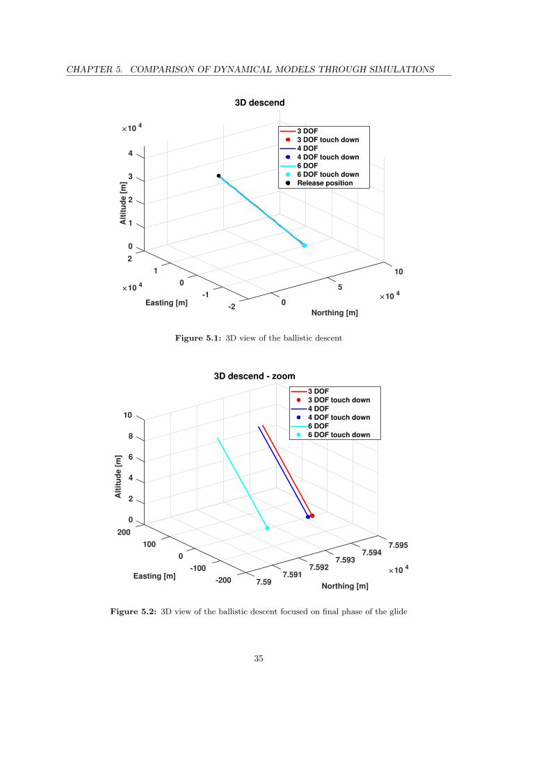
CHAPTER 5. COMPARISON OF DYNAMICAL MODELS THROUGH SIMULATIONS
3D descend
0
5
10
Northing [m]
10 4
-2
-1
0
1
2
Easting [m]
10 4
0
1
2
3
4
Alt
itu
de
[m
]10 4
3 DOF
3 DOF touch down
4 DOF
4 DOF touch down
6 DOF
6 DOF touch down
Release position
Figure 5.1: 3D view of the ballistic descent
3D descend - zoom
7.597.591
7.5927.593
7.5947.595
Northing [m]
10 4
-200
-100
0
100
200
Easting [m]
0
2
4
6
8
10
Alt
itu
de
[m
]
3 DOF
3 DOF touch down
4 DOF
4 DOF touch down
6 DOF
6 DOF touch down
Figure 5.2: 3D view of the ballistic descent focused on final phase of the glide
35
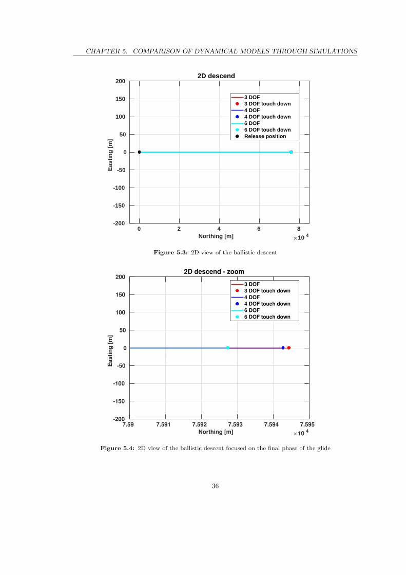
CHAPTER 5. COMPARISON OF DYNAMICAL MODELS THROUGH SIMULATIONS
0 2 4 6 8Northing [m] 10 4
-200
-150
-100
-50
0
50
100
150
200
Eas
tin
g [
m]
2D descend
3 DOF3 DOF touch down4 DOF4 DOF touch down6 DOF6 DOF touch downRelease position
Figure 5.3: 2D view of the ballistic descent
7.59 7.591 7.592 7.593 7.594 7.595
Northing [m] 10 4
-200
-150
-100
-50
0
50
100
150
200
Easti
ng
[m
]
2D descend - zoom
3 DOF
3 DOF touch down
4 DOF
4 DOF touch down
6 DOF
6 DOF touch down
Figure 5.4: 2D view of the ballistic descent focused on the final phase of the glide
36

CHAPTER 5. COMPARISON OF DYNAMICAL MODELS THROUGH SIMULATIONS
0 2000 4000 6000 8000Time [s]
3
4
5
6
7
8
9
10
11
12
Vel
oci
ty [
m/s
]
Vertical velocity
3 DOF3 DOF touch down4 DOF4 DOF touch down6 DOF6 DOF touch down
Figure 5.5: Vertical velocity along the ballistic glide
7300 7320 7340 7360 7380 7400Time [s]
3.3
3.35
3.4
3.45
Vel
oci
ty [
m/s
]
Vertical velocity - zoom
3 DOF3 DOF touch down4 DOF4 DOF touch down6 DOF6 DOF touch down
Figure 5.6: Vertical velocity along the ballistic glide focused on the final phase of the descent
37

CHAPTER 5. COMPARISON OF DYNAMICAL MODELS THROUGH SIMULATIONS
0 2000 4000 6000 8000Time [s]
6
8
10
12
14
16
18
20
Vel
oci
ty [
m/s
]
Horizontal velocity
3 DOF3 DOF touch down4 DOF4 DOF touch down6 DOF6 DOF touch down
Figure 5.7: Horizontal velocity along the ballistic glide
7300 7320 7340 7360 7380 7400Time [s]
6.3
6.35
6.4
6.45
6.5
6.55
6.6
Vel
oci
ty [
m/s
]
Horizontal velocity - zoom
3 DOF3 DOF touch down4 DOF4 DOF touch down6 DOF6 DOF touch down
Figure 5.8: Horizontal velocity along the ballistic glide focused on the final phase of the descent
38

CHAPTER 5. COMPARISON OF DYNAMICAL MODELS THROUGH SIMULATIONS
0 2000 4000 6000 8000Time [s]
1.88
1.885
1.89
1.895
1.9
1.905
1.91
1.915
1.92E
ffic
ien
cyL over D
3 DOF4 DOF6 DOF
Figure 5.9: Lift-to-Drag ratio along the ballistic glide
0 2000 4000 6000 8000Time [s]
25
25.5
26
26.5
27
27.5
28
28.5
29
29.5
30
[d
eg]
Angle of attack
4 DOF6 DOF
Figure 5.10: Angle of attack along the ballistic glide
39

CHAPTER 5. COMPARISON OF DYNAMICAL MODELS THROUGH SIMULATIONS
0 2000 4000 6000 8000Time [s]
-28
-27.9
-27.8
-27.7
-27.6
-27.5
-27.4
-27.3
-27.2
-27.1
-27
a [
deg
]
Flight path angle
3 DOF4 DOF6 DOF
Figure 5.11: Flight path angle along the ballistic glide
-2
2
-2
0
00
Northing [m]
104
104
Easting [m]
104
Alt
itu
de
[m
]
2-2
3D descend
2
4
-4 6
4
3 DOF3 DOF touch down4 DOF4 DOF touch down6 DOF6 DOF touch downRelease position
Figure 5.12: 3D view of the descent with bank actuation
40

CHAPTER 5. COMPARISON OF DYNAMICAL MODELS THROUGH SIMULATIONS
-4 -3 -2 -1 0 1 2Northing [m] 10 4
-1
0
1
2
3
4
5
Eas
tin
g [
m]
10 4 2D descend
3 DOF3 DOF touch down4 DOF4 DOF touch down6 DOF6 DOF touch downRelease position
Figure 5.13: 2D view of the descent with bank actuation
0 2000 4000 6000 8000
Time [s]
3
4
5
6
7
8
9
10
11
12
Velo
cit
y [
m/s
]
Vertical velocity
3 DOF
3 DOF touch down
4 DOF
4 DOF touch down
6 DOF
6 DOF touch down
Figure 5.14: Vertical velocity along the coast with bank actuation
41

CHAPTER 5. COMPARISON OF DYNAMICAL MODELS THROUGH SIMULATIONS
950 1000 1050 1100 1150Time [s]
7
7.5
8
8.5
Vel
oci
ty [
m/s
]
Vertical velocity - zoom
3 DOF3 DOF touch down4 DOF4 DOF touch down6 DOF6 DOF touch down
Figure 5.15: Vertical velocity along the coast with bank actuation focused on the actuation phase
0 2000 4000 6000 8000
Time [s]
6
8
10
12
14
16
18
20
Ve
loc
ity
[m
/s]
Horizontal velocity
3 DOF
3 DOF touch down
4 DOF
4 DOF touch down
6 DOF
6 DOF touch down
Figure 5.16: Horizontal velocity along the coast with bank actuation
42

CHAPTER 5. COMPARISON OF DYNAMICAL MODELS THROUGH SIMULATIONS
950 1000 1050 1100 1150
Time [s]
13.8
14
14.2
14.4
14.6
14.8
15V
elo
cit
y [
m/s
]
Horizontal velocity - zoom
3 DOF3 DOF touch down4 DOF4 DOF touch down6 DOF6 DOF touch down
Figure 5.17: Horizontal velocity along the coast with bank actuation focused on the actuation phase
950 1000 1050 1100 1150Time [s]
1.8965
1.897
1.8975
1.898
1.8985
1.899
1.8995
1.9
Eff
icie
ncy
L over D
3 DOF4 DOF6 DOF
Figure 5.18: Lift-to-Drag ratio along the coast with bank actuation focused on the actuation phase
43
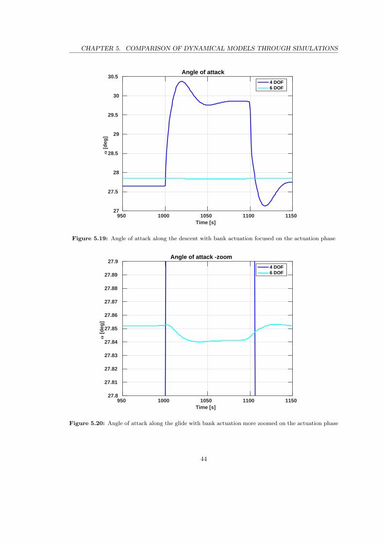
CHAPTER 5. COMPARISON OF DYNAMICAL MODELS THROUGH SIMULATIONS
950 1000 1050 1100 1150Time [s]
27
27.5
28
28.5
29
29.5
30
30.5
[d
eg]
Angle of attack
4 DOF6 DOF
Figure 5.19: Angle of attack along the descent with bank actuation focused on the actuation phase
950 1000 1050 1100 1150Time [s]
27.8
27.81
27.82
27.83
27.84
27.85
27.86
27.87
27.88
27.89
27.9
[d
eg]
Angle of attack -zoom
4 DOF6 DOF
Figure 5.20: Angle of attack along the glide with bank actuation more zoomed on the actuation phase
44

CHAPTER 5. COMPARISON OF DYNAMICAL MODELS THROUGH SIMULATIONS
0 2000 4000 6000 8000Time [s]
0
20
40
60
80
100
120
140
160
a [
deg
]
Heading angle
3 DOF4 DOF6 DOF
Figure 5.21: Heading angle along the descent with bank actuation
0 2000 4000 6000 8000Time [s]
0
2
4
6
8
10
12
14
16
18
a [
deg
]
Bank angle
3 DOF4 DOF6 DOF
Figure 5.22: Bank angle along the descent with bank actuation
45

CHAPTER 5. COMPARISON OF DYNAMICAL MODELS THROUGH SIMULATIONS
950 1000 1050 1100 1150Time [s]
0
2
4
6
8
10
12
14
16
18
a[d
eg]
Bank angle - zoom
3 DOF4 DOF6 DOF
Figure 5.23: Bank angle along the descent with bank actuation focused on the actuation phase
0 2000 4000 6000 8000
Time [s]
-30
-29.5
-29
-28.5
-28
-27.5
-27
a [
deg
]
Flight path angle
3 DOF
4 DOF
6 DOF
Figure 5.24: Flight path angle along the descent with bank actuation
46

Chapter 6
Sensitivity analysis on the 6 DOFmodel
Once that all models have been compared and understood, a sensitivity analysis on geometricalparameters of the parafoil can be conducted. The wind will not be considered in these simulations.Firstly a simulation of a not actuated descent will be carried out and analyzed and then anactuated case will be presented. Geometrical parameters on which the sensitivity analysis will beperformed and their nominal values are: canopy area (Snom = 3.144 m2), aspect ratio (ARnom =3), rigging angle (µnom = −12 deg), line length (Rnom = 1.843 m), and payload mass (mnom =200 kg). All these parameters will be let varying from 0.1 to 10 times the nominal value whenpossible. An exception will be done for the payload mass, since the use of values from 100 kgto 500 kg has been expressively requested. In order to be consistent during the whole analysisand through different steps and to help the immediate understanding of graphs, the nominalcondition will be always presented with a red point. Some setbacks happened during this phaseof the work: for certain values of a parameter (typically a value very distant from the nominalone) the simulation became unstable, Matlab was no more capable of integrate and time historyof each variable was incorrect. This is due to the fact that aerodynamic coefficients and actuationparameters are suited for the nominal case; therefore, this fact could happen. For each case themaximum and minimum value for which the simulation can be run will be written; when notspecified, maximum and minimum acceptable values are 0.1 and 10 times the nominal one. Thisprocedure is useful to understand boundaries inside which this model works well and can be usedappropriately. Also in this case, the numerical integration has been performed with the ode15sMatlab routine.
6.1 Ballistic descent
Performance parameters for which the variation after the parafoil geometry change will be in-vestigated are: gliding range (∆x), descent time (∆T ), vertical touchdown velocity (Vz0) andhorizontal touchdown velocity (Vh0
). Results are summarized in following paragraphs.
6.1.1 Canopy area variation
With increasing canopy area:
• Gliding range increases (it always assume almost the value hreleaseLD ) (Figure 6.1);
47

CHAPTER 6. SENSITIVITY ANALYSIS ON THE 6 DOF MODEL
• Descent time increases (Figure 6.2);
• Vertical and horizontal touchdown velocity decrease (Figures 6.3 and 6.4).
6.1.2 Aspect ratio variation
With increasing aspect ratio, all interesting performances remain almost constant, since theshape of the parafoil (not the total surface but how this surface is shaped) acts an importantrole only during maneuvers. Since variation from nominal condition are not present, plots havenot been reported.
6.1.3 Rigging angle variation
The rigging angle µ has been varied from -5 to 5 times the nominal value, since having a riggingangle greater than 90 deg has no meaning. The rigging angle variation causes changes in inertiavalues; since in a ballistic descent these numbers are not involved, the rigging angle changingdoes not produce any effect on performances of interest; for this reason plots have not beenreported.
6.1.4 Line length variation
With increasing line length, all interesting performances remain almost constant, since this valueaffect inertia values which act an important role only during maneuvers. Since variation fromnominal condition are not present, plots have not been reported.
6.1.5 Payload mass variation
With increasing payload mass:
• Gliding range decreases, but its variation is small compared with the mass variation (Figure6.5);
• Descent time increases (Figure 6.6);
• Vertical and horizontal touchdown velocity increase (Figures 6.7 and 6.8).
6.2 Actuated descent
Performance parameters for which the variation after the parafoil geometry change will be inves-tigated are: descent time (∆T ), vertical touchdown velocity (Vz0), horizontal touchdown velocity(Vh0) and amount of heading angle variation (∆χa). Simulation results show that trend of vari-ation of ∆T , Vz0 and Vh0
are equal to the one presented in section 6.1 for a ballistic descent; forthis reason, no more considerations and graphical results will be given upon them along this sec-tion. Attention will be focused on how much the parafoil is able to turn with the same actuationchanging parafoil geometrical parameters. Results are summarized in following paragraphs.
48

CHAPTER 6. SENSITIVITY ANALYSIS ON THE 6 DOF MODEL
6.2.1 Canopy area variation
With increasing canopy area, the total amount of heading angle variation decreases; the biggeris the parafoil, the less it turns in response to the same actuation. Figure 6.9 shows this trend,while Figure 6.10 exhibits the 3D trajectory for different canopy areas. The maximum value ofS for which the simulation does not go crazy is Smax = 7.20 m2; for a canopy 10 times smallerthan the nominal one the simulation does not show any issue.
6.2.2 Aspect ratio variation
With increasing aspect ratio, the total amount of heading angle variation decreases. Figure 6.11shows this trend, while Figure 6.12 exhibits the 3D trajectory for different aspect ratio. Themaximum and minimum values of AR for which the simulation does not become unstable areARmin = 0.64 and ARmax = 19.65.
6.2.3 Rigging angle variation
Since µ variation does not have a great effect on the bank angle produced by the actuation,performances of interest do not change so much varying it. Total amount of heading anglevariation slightly changes, such that the turn capability is minimum for the reference condition(µ = −12 deg) and is higher for lower and upper values. For µ = −60 deg the behavior is quitedifferent (turn capability increases of some degrees) but it is quite impossible to build a parafoilwith this rigging angle (usually this angle has a small value). Figure 6.13 shows this trend, whileFigure 6.14 exhibits the 3D trajectory for different rigging angle. The simulation is stable for allvalues of rigging angle from −0.6 deg to −60 deg.
6.2.4 Line length variation
Having different R values produces a variation in parafoil inertia matrix terms (the bigger is linelength, the bigger are inertia values). Therefore, increasing R the total amount of heading anglevariation decreases. Figure 6.15 shows this trend, while Figure 6.16 exhibits the 3D trajectoryfor different line length. The maximum value of R for which the simulation does not go crazy isRmax = 10.05 m; for a line length 10 times less than the nominal one the simulation does notshow any issue.
6.2.5 Payload mass variation
Increasing the payload mass, the produced bank angle increases; hence the total amount ofheading angle variation does the same. Figure 6.17 shows this trend, while Figure 6.18 exhibitsthe 3D trajectory for different payload mass. The simulation does not show instability behaviorfor any value inside the range of mass 100 kg - 500 kg.
49

CHAPTER 6. SENSITIVITY ANALYSIS ON THE 6 DOF MODEL
0 5 10 15 20 25 30 35Canopy area [m^2]
73
73.5
74
74.5
75
75.5
76
76.5
Glid
ing
ran
ge
[km
]
Gliding range vs canopy area
S=0.3144 m^2S=0.6288 m^2S=3.144 m^2S=15.72 m^2S=31.44 m^2
Figure 6.1: Gliding range change with canopy area variation
0 5 10 15 20 25 30 35Canopy area [m^2]
0
50
100
150
200
250
300
350
400
Des
cen
t ti
me
[min
]
Total descent time vs canopy area
S=0.3144 m^2S=0.6288 m^2S=3.144 m^2S=15.72 m^2S=31.44 m^2
Figure 6.2: Descent time change with canopy area variation
50

CHAPTER 6. SENSITIVITY ANALYSIS ON THE 6 DOF MODEL
0 5 10 15 20 25 30 35Canopy area [m^2]
1
2
3
4
5
6
7
8
9
10
11
Vz [
m/s
]
Vertical touchdown velocity vs canopy area
S=0.3144 m^2S=0.6288 m^2S=3.144 m^2S=15.72 m^2S=31.44 m^2
Figure 6.3: Vertical touchdown velocity change with canopy area variation
0 5 10 15 20 25 30 35
Canopy area [m^2]
2
4
6
8
10
12
14
16
18
20
22
Vh [
m/s
]
Horizontal touchdown velocity vs canopy area
S=0.3144 m^2S=0.6288 m^2
S=3.144 m^2S=15.72 m^2
S=31.44 m^2
Figure 6.4: Horizontal touchdown velocity change with canopy area variation
51

CHAPTER 6. SENSITIVITY ANALYSIS ON THE 6 DOF MODEL
100 200 300 400 500Payload mass [kg]
75.55
75.6
75.65
75.7
75.75
75.8
75.85
75.9
75.95
76
76.05
Glid
ing
ran
ge
[km
]
Gliding range vs payload mass
m=100 kgm=200 kgm=300 kgm=400 kgm=500 kg
Figure 6.5: Gliding range change with payload mass variation
100 200 300 400 500Payload mass [kg]
60
80
100
120
140
160
180
Des
cen
t ti
me
[min
]
Total descent time vs payload mass
m=100 kgm=200 kgm=300 kgm=400 kgm=500 kg
Figure 6.6: Descent time change with payload mass variation
52

CHAPTER 6. SENSITIVITY ANALYSIS ON THE 6 DOF MODEL
100 200 300 400 500Payload mass [kg]
2
2.5
3
3.5
4
4.5
5
5.5
Vz [
m/s
]
Vertical touchdown velocity vs payload mass
m=100 kgm=200 kgm=300 kgm=400 kgm=500 kg
Figure 6.7: Vertical touchdown velocity change with payload mass variation
100 200 300 400 500
Payload mass [kg]
4
5
6
7
8
9
10
11
Vh
[m
/s]
Horizontal touchdown velocity vs payload mass
m=100 kg
m=200 kg
m=300 kg
m=400 kg
m=500 kg
Figure 6.8: Horizontal touchdown velocity change with payload mass variation
53

CHAPTER 6. SENSITIVITY ANALYSIS ON THE 6 DOF MODEL
0 2 4 6 8
Canopy area [m^2]
0
200
400
600
800
1000
1200
a [
de
g]
Amount of heading angle variation vs canopy area
S=0.3144 m^2S=0.6288 m^2
S=3.144 m^2S=5.172 m^2
S=7.2 m^2
Figure 6.9: Amount of turn change with canopy area variation
0
Easting [m]
1045
-1
Descending trajectory at different canopy area values
Northing [m]10
4
0
105 10
1
0
Alt
itu
de
[m
]
104
-5
2
3
4
S=0.3144 m^2S=0.6288 m^2
S=3.144 m^2S=5.172 m^2
S=7.2 m^2
Figure 6.10: 3D trajectory with canopy area variation
54
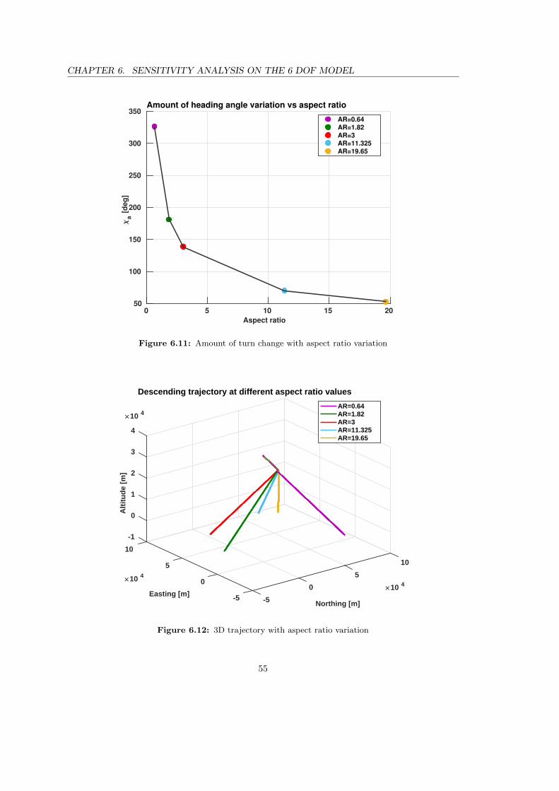
CHAPTER 6. SENSITIVITY ANALYSIS ON THE 6 DOF MODEL
0 5 10 15 20
Aspect ratio
50
100
150
200
250
300
350
a [
deg
]
Amount of heading angle variation vs aspect ratio
AR=0.64
AR=1.82
AR=3
AR=11.325
AR=19.65
Figure 6.11: Amount of turn change with aspect ratio variation
-1
0
10
1
10
2
10 4
Alt
itu
de
[m]
5
Descending trajectory at different aspect ratio values
3
10 4
Easting [m]
5
10 4
Northing [m]
4
00
-5 -5
AR=0.64AR=1.82AR=3AR=11.325AR=19.65
Figure 6.12: 3D trajectory with aspect ratio variation
55

CHAPTER 6. SENSITIVITY ANALYSIS ON THE 6 DOF MODEL
-60 -50 -40 -30 -20 -10 0
Rigging angle [deg]
138
138.5
139
139.5
140
140.5
141
141.5
142
142.5
143
a [
deg
]
Amount of heading angle variation vs rigging angle
=-2.4 deg
=-4.8 deg
=-12 deg
=-30 deg
=-60 deg
Figure 6.13: Amount of turn change with rigging angle variation
-1
0
2
1
0
2
Alt
itu
de
[m]
10 4
0
Descending trajectory at different rigging angle values
1
3
10 4
Northing [m]Easting [m]
10 4
4
2-23
-4 4
=-2.4 deg=-4.8 deg=-12 deg=-30 deg=-60 deg
Figure 6.14: 3D trajectory with rigging angle variation
56

CHAPTER 6. SENSITIVITY ANALYSIS ON THE 6 DOF MODEL
0 2 4 6 8 10 12Line length [m]
134
135
136
137
138
139
140
a [
deg
]
Amount of heading angle variation vs line length
R=0.1843 mR=1.0136 mR=1.843 mR=5.9465 mR=10.05 m
Figure 6.15: Amount of turn change with line length variation
-1
2
0
0
1
0 2
10 4
Alt
itu
de
[m]
10 4
Northing [m]
2
Descending trajectory at different line length values
10 4
Easting [m]
3
-2 4
4
-4 6
R=0.1843 mR=1.0136 mR=1.843 mR=5.9465 mR=10.05 m
Figure 6.16: 3D trajectory with line length variation
57

CHAPTER 6. SENSITIVITY ANALYSIS ON THE 6 DOF MODEL
100 200 300 400 500Payload mass [kg]
100
120
140
160
180
200
220
a [
deg
]
Amount of heading angle variation vs payload mass
m=100 kgm=200 kgm=300 kgm=400 kgm=500 kg
Figure 6.17: Amount of turn change with payload mass variation
-1
4
0
1
2-5
2
Alt
itu
de
[m]
10 4
10 4
Northing [m]
0
Descending trajectory at different payload mass values
3
0
Easting [m]
10 4-2
4
5-4 10
m=100 kgm=200 kgm=300 kgm=400 kgm=500 kg
Figure 6.18: 3D trajectory with payload mass variation
58

Chapter 7
Wind drift simulations
As already said, the wind is the greatest parafoils enemy. Since parafoil velocity is not so highand it can assume values comparable to wind ones, the effect of wind on parafoil trajectory has tobe investigated. First of all, a wind model variable with height will be introduced, then differentsimulations will be carried out. Results of simulations (performed with the 6 DOF model) withdifferent wind condition (lateral towards east and towards west, longitudinal from behind andfrom in front, ballistic and actuated case) will be presented. For what concerns vertical wind,in [25] is said that expected values are very small and that generally it can be neglected. Thereis however the possibility (< 0.5%) of encountering a wind with velocity 1− 10 m/s. Results ofa simulation with +1 m/s and −1 m/s vertical wind in both ballistic and actuated case will bepresented (actuation condition is the same presented in section 5.3). Numerical integration is asalways performed with the ode15s Matlab routine.
7.1 Titan drift wind model
A suitable wind model for Titan atmosphere has to be carried out in order to simulate the descentof a parafoil considering this effect. According to [25] a good medium wind model can be:
w(h) =25
1 + exp 38−h11
(7.1)
with altitude in km and wind velocity in m/s. This model will be used for the simulation withlateral and longitudinal wind. Regarding the situation of a longitudinal wind from behind, thesimulation becomes unstable for a numerator greater than 18 in the wind model; for this reasonresults are given for this maximum value. Figure 7.1 shows the comparison between the nominalwind profile and the maximum possible frontal wind profile.
7.2 Lateral wind
7.2.1 Ballistic trajectory
Effects of eastward or westward wind on a ballistic trajectory can be summarized in followingconsiderations:
• The trajectory changes: a positive or negative drift of 38.4 km on the landing position dueto the wind is present (Figures 7.2 and 7.3).
59

CHAPTER 7. WIND DRIFT SIMULATIONS
0 1 2 3 4h [m] 10 4
0
2
4
6
8
10
12
14
Win
d v
elo
city
[m
/s]
Nominal medium wind vs implemented frontal wind
nominal medium windpossible frontal wind
Figure 7.1: Comparison between nominal wind and implemented frontal maximum wind
• The horizontal touchdown velocity changes: it has the minimum value for the no windcondition (Figure 7.4).
• The vertical touchdown velocity does not change as well as the descent time, since nothinghas been varied in the vertical dynamics.
7.2.2 Actuated trajectory
Effects of eastward or westward wind on an actuated trajectory can be summarized in followingconsiderations:
• The trajectory is affected by the wind: the maneuver (and so the amount of turn given bythe actuation) depends on the wind condition (Figures 7.5 and 7.6).
• The horizontal touchdown velocity changes: it has the minimum value for the -east windcondition (this fact is strictly related to the specific simulated condition, since it is suchthat the parafoil flies upwind for the -east wind condition) (Figure 7.7).
• Descent time varies because different wind conditions during the maneuver mean a differentheight loss: operate a turn towards wind means having higher height loss and so smallerdescent time (Figure 7.8).
• The vertical touchdown velocity and the descent time do not change.
7.3 Longitudinal wind
7.3.1 Ballistic trajectory
Effects of longitudinal wind (in front or from behind) on a ballistic trajectory can be summarizedin following considerations:
60

CHAPTER 7. WIND DRIFT SIMULATIONS
• The trajectory changes: the gliding range increases or decreases depending on the directionof the wind (Figures 7.9 and 7.10).
• The horizontal touchdown velocity changes: it has the same trend of the gliding range(Figure 7.11).
• The vertical touchdown velocity does not change and the descent time does the same, sincenothing has been varied in the vertical dynamics.
7.3.2 Actuated trajectory
Effects of longitudinal wind (in front or from behind) on an actuated trajectory can be summa-rized in following considerations:
• The trajectory is affected by the wind: the maneuver (and so the amount of turn given bythe actuation) depends on the wind condition (Figures 7.12 and 7.13).
• The horizontal touchdown velocity changes: the direction taken after the maneuver is suchthat the horizontal touchdown velocity is greater for the in front wind condition (this factis valid for this precise maneuver: different actuation may have different results in thisprecise point) (Figure 7.14).
• Descent time varies because different wind condition during the maneuver means differentheight loss: starting the maneuver flying in the direction of the wind produces an higherheight loss (and so a lower descent time) (Figure 7.15).
• The vertical touchdown velocity and the descent time do not change, since nothing hasbeen varied in the vertical dynamics.
7.4 Vertical wind
7.4.1 Ballistic trajectory
Effects of vertical wind on a ballistic trajectory can be summarized in following considerations:
• The trajectory changes: the gliding range increases or decreases depending on the directionof the wind (Figures 7.16 and 7.17).
• The horizontal touchdown velocity does not change, since nothing has been varied in thehorizontal dynamics.
• The vertical touchdown velocity and the descent time change: they increase or decreasedepending on the wind direction (Figures 7.18 and 7.19).
7.4.2 Actuated trajectory
Effects of vertical wind on an actuated trajectory can be summarized in following considerations:
• The trajectory is affected by the wind, since its presence changes the altitude at which themaneuver is performed and changes the trajectory after the maneuver (Figures 7.20 and7.21).
• Horizontal and vertical touchdown velocity and descent time vary exactly as in the ballisticcase just described: for this reason graphical representation of them will not be reported.
61

CHAPTER 7. WIND DRIFT SIMULATIONS
7.5 Considerations
Some general comments about these analysis have to be made:
• The wind has the effect of drifting the parafoil away from its nominal trajectory, changingthe landing position and touchdown performances. Is there a way to compensate thiseffect?
• The worst condition that parafoil has to face is the lateral wind, since the drift of thetrajectory is in the order of 40 km. This number makes us understand that this effect mustbe counteracted in such a way.
• Longitudinal and vertical wind have effects on gliding range and descent time. These issuescan be in a sort of way mitigated with a gliding angle control (symmetric actuation).
How to deal with the effect of a lateral blast of wind will be explained in section 10.4 and answerto the first bullet point question will be investigated.
62

CHAPTER 7. WIND DRIFT SIMULATIONS
-1
0
0 5
1
2
104
Alt
itu
de
[m
]
3D trajectory - changing lateral wind
Northing [m]
104
Easting [m]
104
3
5 0
4
10 -5
No wind
+East wind
-East wind
Figure 7.2: 3D view of ballistic trajectory with different lateral wind conditions
0 2 4 6 8Northing [m] 10 4
-4
-3
-2
-1
0
1
2
3
4
Eas
tin
g [
m]
10 4 2D trajectory - changing lateral wind
No wind+East wind-East wind
Figure 7.3: 2D view of ballistic trajectory with different lateral wind conditions
63

CHAPTER 7. WIND DRIFT SIMULATIONS
-1 -0.5 0 0.5 1Lateral wind at zero altitude [m/s]
6.4
6.42
6.44
6.46
6.48
6.5
6.52
6.54
6.56
6.58
6.6
Ho
rizo
nta
l vel
oci
ty a
t ze
ro a
ltit
ud
e [m
/s]
Horizontal velocity - changing lateral wind
No wind+East wind-East wind
Figure 7.4: Horizontal touchdown velocity with different lateral wind conditions
-1
2 -5
0
1
0 0
Northing [m]
104
Easting [m]
104
Alt
itu
de
[m
]
104
3D trajectory - changing lateral wind
2
-2 5
3
-4 10
4
No wind
+East wind
-East wind
Figure 7.5: 3D view of actuated trajectory with different lateral wind conditions
64

CHAPTER 7. WIND DRIFT SIMULATIONS
-4 -3 -2 -1 0 1 2Northing [m] 10 4
-2
-1
0
1
2
3
4
5
6
7
Eas
tin
g [
m]
10 4 2D trajectory - changing lateral wind
No wind+East wind-East wind
Figure 7.6: 2D view of actuated trajectory with different lateral wind conditions
-1 -0.5 0 0.5 1Lateral wind at zero altitude [m/s]
5.8
6
6.2
6.4
6.6
6.8
7
Ho
rizo
nta
l vel
oci
ty a
t ze
ro a
ltit
ud
e [m
/s]
Horizontal velocity - changing lateral wind
No wind+East wind-East wind
Figure 7.7: Horizontal touchdown velocity with different lateral wind conditions
65
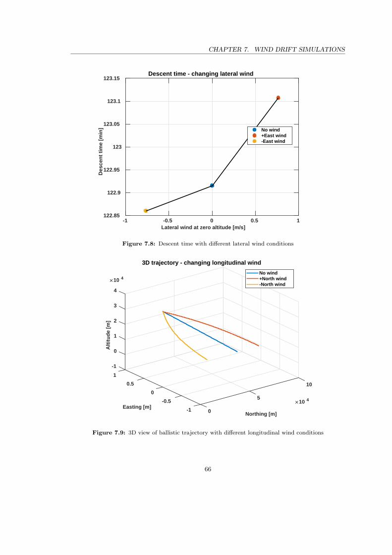
CHAPTER 7. WIND DRIFT SIMULATIONS
-1 -0.5 0 0.5 1Lateral wind at zero altitude [m/s]
122.85
122.9
122.95
123
123.05
123.1
123.15
Des
cen
t ti
me
[min
]
Descent time - changing lateral wind
No wind+East wind-East wind
Figure 7.8: Descent time with different lateral wind conditions
3D trajectory - changing longitudinal wind
0
5
10
Northing [m]
10 4
-1
-0.5
0
0.5
1
Easting [m]
-1
0
1
2
3
4
Alt
itu
de
[m]
10 4No wind+North wind-North wind
Figure 7.9: 3D view of ballistic trajectory with different longitudinal wind conditions
66

CHAPTER 7. WIND DRIFT SIMULATIONS
0 2 4 6 8 10Northing [m] 10 4
-0.5
0
0.5
1
1.5
2
2.5
3
3.5
4
Alt
itu
de
[m]
10 4 2D trajectory - changing longitudinal wind
No wind+North wind-North wind
Figure 7.10: 2D view of ballistic trajectory with different longitudinal wind conditions
-1 -0.5 0 0.5Longitudinal wind at zero altitude [m/s]
5.5
6
6.5
7
7.5
Ho
rizo
nta
l vel
oci
ty a
t ze
ro a
ltit
ud
e [m
/s]
Horizontal velocity - changing longitudinal wind
No wind+North wind-North wind
Figure 7.11: Horizontal touchdown velocity with different longitudinal wind conditions
67

CHAPTER 7. WIND DRIFT SIMULATIONS
0
1-1
0
510
4
Easting [m]
2
3D trajectory - changing longitudinal wind
1
104
Northing [m]
0
Alt
itu
de
[m
]10
4
2
3-5
3
4
4
-10
No wind
+North wind
-North wind
Figure 7.12: 3D view of actuated trajectory with different longitudinal wind conditions
-6 -4 -2 0 2 4Northing [m] 10 4
0
0.5
1
1.5
2
2.5
3
3.5
4
Eas
tin
g [
m]
10 4 2D trajectory - changing longitudinal wind
No wind+North wind-North wind
Figure 7.13: 2D view of actuated trajectory with different longitudinal wind conditions
68

CHAPTER 7. WIND DRIFT SIMULATIONS
-0.8 -0.6 -0.4 -0.2 0 0.2 0.4 0.6Longitudinal wind at zero altitude [m/s]
6
6.2
6.4
6.6
6.8
7
7.2
Ho
rizo
nta
l vel
oci
ty a
t ze
ro a
ltit
ud
e [m
/s]
Horizontal velocity - changing longitudinal wind
No wind+North wind-North wind
Figure 7.14: Horizontal touchdown velocity with different longitudinal wind conditions
-0.5 0 0.5Longitudinal wind at zero altitude [m/s]
122
122.2
122.4
122.6
122.8
123
123.2
123.4
123.6
123.8
124
Des
cen
t ti
me
[min
]
Descent time - changing longitudinal wind
No wind+North wind-North wind
Figure 7.15: Descent time with different longitudinal wind conditions
69

CHAPTER 7. WIND DRIFT SIMULATIONS
3D trajectory - changing vertical wind
0
5
10
Northing [m]
10 4
-1
-0.5
0
0.5
1
Easting [m]
0
1
2
3
4A
ltit
ud
e [m
]
10 4No windDown windUp wind
Figure 7.16: 3D view of ballistic trajectory with different vertical wind conditions
0 2 4 6 8 10Northing [m] 10 4
0
0.5
1
1.5
2
2.5
3
3.5
4
Alt
itu
de
[m]
10 4 2D trajectory - changing vertical wind
No windDown windUp wind
Figure 7.17: 2D view of ballistic trajectory with different vertical wind conditions
70

CHAPTER 7. WIND DRIFT SIMULATIONS
-1 -0.5 0 0.5 1Vertical wind at zero altitude [m/s]
100
110
120
130
140
150
160D
esce
nt
tim
e [m
in]
Descent time - changing vertical wind
Up windNo windDown wind
Figure 7.18: Descent time with different vertical wind conditions
-1 -0.5 0 0.5 1Vertical wind at zero altitude [m/s]
2
2.5
3
3.5
4
4.5
Ver
tica
l vel
oci
ty a
t ze
ro a
ltit
ud
e [m
/s]
Vertical velocity - changing vertical wind
No windDown windUp wind
Figure 7.19: Vertical touchdown velocity with different vertical wind conditions
71

CHAPTER 7. WIND DRIFT SIMULATIONS
0
1-1
22
Easting [m]
10 4
0
0 3
3D trajectory - changing vertical wind
Northing [m]
10 4
1
-2
10 4A
ltit
ud
e [
m]
4
2
-45
3
-6
4
No wind
Down wind
Up wind
Figure 7.20: 3D view of actuated trajectory with different vertical wind conditions
-5 -4 -3 -2 -1 0 1 2Northing [m] 10 4
-0.5
0
0.5
1
1.5
2
2.5
3
3.5
4
Alt
itu
de
[m]
10 4 2D trajectory - changing vertical wind
No windDown windUp wind
Figure 7.21: 2D view of actuated trajectory with different vertical wind conditions
72

Chapter 8
Dynamical model refinement
The 6 DOF model discussed in [2, cha. 5] and here introduced in section 3.1.5 does not considersome small effects which can affect the dynamics of the parafoil during a Titan descent. In thischapter they will be described and discussed; an estimation of their order of magnitude willbe performed and then the decision of retrieving or discarding them will be taken. They are:buoyancy force, centrifugal acceleration, transport acceleration and Coriolis acceleration.
8.1 Buoyancy force
Buoyancy force acts in the direction of the weight but in the opposite versus. It is small comparedto the weight force but, since it is applied at the point of reference of the canopy and not at thecenter of mass of the system, it plays an important role significantly contributing to the balanceof moments. Its expression, according to [6, cha. 4.6], is:
B = −gmadded (8.1)
Since it acts in the direction of weight, exactly as Fg, the vector
FB = B
sin(θ)cos(θ) sin(φ)cos(θ) cos(φ)
(8.2)
will be added to B1 vector of equation (3.19). Regarding the contribution to moment equation(equation (3.20)), the term MB will be added to it as:
MB =
00rpz
× FB (8.3)
where rpz is the distance between point of reference of the canopy and center of mass of thesystem. Buoyancy force will be inserted in the model because of its effect in the moment equation;but to evaluate its order of magnitude it will be compared to weight in the force equation. Forthe nominal case (m = 200 kg, S = 3.144 m2, AR = 3 and so on) the buoyancy force at zeroaltitude (where its value is the highest since added mass increases linearly with density) is:
B = 0.09bc2gρ = 2.124 N (8.4)
73

CHAPTER 8. DYNAMICAL MODEL REFINEMENT
The weight force has the value of:
|Fg| = mg = 270.4 N (8.5)
Computing the ratio between them the buoyancy force results to be the 0.79% of the weight.It will be retained and inserted in equations of motion (especially because of its contributionto moment equation, since its application point is not the center of mass). Inserting buoyancyforce in the model and running a simulation without any actuation the descent time passes from122.99 min to 123.16 min and the touchdown velocity passes from 3.393 m/s to 3.379 m/s: asexpected buoyancy has the effect of decelerating the descent and of increasing the total neededtime to reach the planetary surface.
8.2 Centrifugal acceleration
The centrifugal acceleration takes the expression:
acentr =V 2
r(8.6)
where V is the ground speed and r is the distance from the center of the planet. Following theprocedure explained in [12, cha. 3.4], centrifugal acceleration has been compared to gravitationalone, remembering that during orbital motion they are equal. Therefore, during an orbital flight,the following equality holds:
Vorbital2
r= g (8.7)
Hence the ration V 2/gr is crucial to decide if discard or retain the centrifugal acceleration; ifthis ratio is 1 the flight speed is too small to give to the centrifugal acceleration a valuecomparable to the gravitational one. For the purposes of this study, the computation will bedone at h = 0 m and h = 35000 m (it is a value that has been taken sufficiently distant from therelease in order not to be affected at all by initial condition given to the integration but still highenough to have a good estimation of centrifugal acceleration at release altitude) considering theworst case scenario: payload mass of 500 kg. At h = 0, computed values from Matlab simulationare: V = 11.52 m/s, r = 2575000 m, g = 1.352 m/s2. Using these numbers:
V 2
gr= 3.81 ∗ 10−5 (8.8)
At h = 35000 m, computed values from Matlab simulation are: V = 28.28 m/s, r = 2610000 m,g = 1.352 m/s2. Using these numbers:
V 2
gr= 2.27 ∗ 10−4 (8.9)
These passages show that centrifugal acceleration is the 0.0038% or the 0.022% of the weightforce in the case of study. Therefore, this effect has been discarded and not inserted in equationsof motion.
8.3 Coriolis and transport acceleration
According to [12, cha. 3.1], assuming that the planet rotates at constant angular velocity ω,equations of motion describing a generic object flying around the planet (in planet fixed inertial
74

CHAPTER 8. DYNAMICAL MODEL REFINEMENT
frame) are:
mdV
dt= F − 2mω × V −mω × (ω × r) (8.10)
where F is the sum of all forces acting on it and V is its velocity; moreover, the term 2ω × Vis the Coriolis acceleration, while the term ω × (ω × r) is the transport acceleration. As donebefore, they have been compared to gravity force in order to understand if they have to beretained or discarded. Titan parameters are: g = 1.352 m/s2, ωTitan = 4.56 ∗ 10−6 rad/sand RTitan = 2575000 m. The considered case is also here the worst one: payload mass of500 kg, altitude of h = 35000 m and V = 28.28 m/s. Starting from the Coriolis acceleration, itsmaximum value is 2ωV . Inserting numbers:
aCoriolis = 2ωV = 2.579 ∗ 10−4 m
s2= 1.908 ∗ 10−4g (8.11)
Since the Coriolis acceleration results to be the 0.019% of the gravitation acceleration, it hasbeen discarded and not inserted in the model. Passing then to the transport acceleration, itsmaximum value is ω2r (it assumes this value when the object is at equatorial plane). Insertingnumbers:
atransport = ω2r = 5.427 ∗ 10−5 m
s2= 4.014 ∗ 10−5g (8.12)
Since the transport acceleration results to be the 0.004% of the gravitation acceleration, it hasnot been inserted in equations of motion.
75

Chapter 9
High fidelity model: 9 DOF
At the beginning of this chapter a question can arise: why is necessary to develop a 9 DOFmodel, since a 6 DOF model is already operative? Two reasons can be find. First of all, inthe 6 DOF model presented in this work the center of mass of the canopy coincides with itsaerodynamic center; for this reason the expected oscillatory behavior of the angle of attack (andof all derived quantities) during the descent cannot be observed; to make it visible, the center ofmass and the aerodynamic center have to be in two different position. In literature ( [2] and [10]),this is done in the 9 DOF model framework and not in the 6 DOF one. But a second reason forthe development of a 9 DOF model has to be underline. Parafoil and payload are two differententities linked together; therefore, they can have relative motion and the payload can respondto asymmetric actuation in a different way with respect to the canopy. To investigate payloadtime story evolution, a 9 DOF model is needed. In this section the high fidelity model will beintroduced and explained; secondly a ballistic reference descent will be simulated and results willbe presented; then a sensitivity analysis (on a ballistic descent) will be performed in order tostudy how simulation results change varying geometrical parafoil parameters.
9.1 Model description
The model which will be described in this section has been derived according to [10]. Theparafoil and the payload are modeled as two separate rigid body linked together. In Figure9.1 a schematic representation of the parafoil can be found. The center of mass of the canopyand the one of the payload are connected to the joint C through rigid massless links. Boththe parafoil and the payload are free to rotate about joint C, but they are constrained by theinternal joint force (Fxc , Fyc , Fzc) at C. The 9 DOF motion of the system is described by 3 inertialposition components of joint C (xc, yc, zc) as well as 3 orientation angles of parafoil (φP , θP , ψP )and payload (φB , θB , ψB). Throughout the description, the subscript P will indicate quantitiesrelative to the parafoil while the subscript B will be used for the payload (B stands for Box).Point of interest for the model description are:
• parafoil mass center (point P): it is assumed to be at parafoil canopy mid-baseline point;
• parafoil aerodynamic center (point AC): it is assumed to be at a distance of xPA from theparafoil center of mass;
• connection point (point C);
• payload center of mass (point B).
77
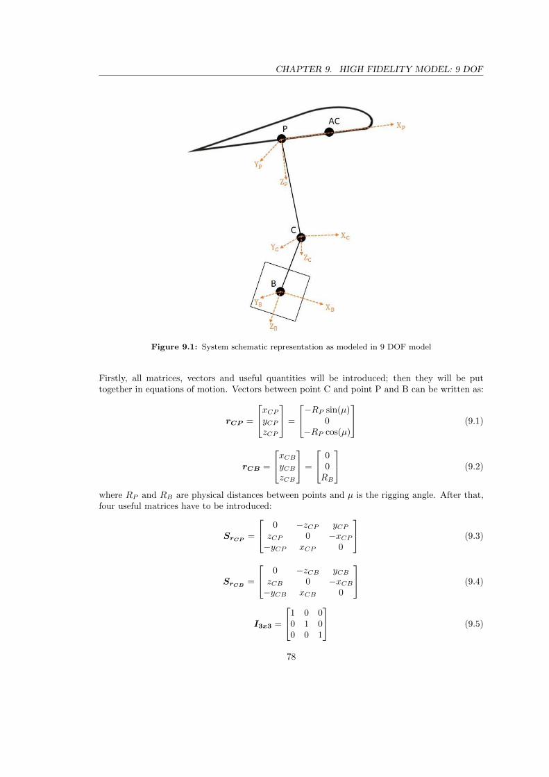
CHAPTER 9. HIGH FIDELITY MODEL: 9 DOF
Figure 9.1: System schematic representation as modeled in 9 DOF model
Firstly, all matrices, vectors and useful quantities will be introduced; then they will be puttogether in equations of motion. Vectors between point C and point P and B can be written as:
rCP =
xCPyCPzCP
=
−RP sin(µ)0
−RP cos(µ)
(9.1)
rCB =
xCByCBzCB
=
00RB
(9.2)
where RP and RB are physical distances between points and µ is the rigging angle. After that,four useful matrices have to be introduced:
SrCP =
0 −zCP yCPzCP 0 −xCP−yCP xCP 0
(9.3)
SrCB =
0 −zCB yCBzCB 0 −xCB−yCB xCB 0
(9.4)
I3x3 =
1 0 00 1 00 0 1
(9.5)
78

CHAPTER 9. HIGH FIDELITY MODEL: 9 DOF
03x3 =
0 0 00 0 00 0 0
(9.6)
Then, angular velocities (of both payload and parafoil) have to be defined (in vector and skew-symmetric matrix form):
ωP =
pPqPrP
(9.7)
ωB =
pBqBrB
(9.8)
ΩP =
0 −rP qPrP 0 −pP−qP pP 0
(9.9)
ΩB =
0 −rB qBrB 0 −pB−qB pB 0
(9.10)
Then groundspeed vector shall be introduced:
VC =
uCvCwC
(9.11)
Now inertia matrix of parafoil (IP ) and of payload (IB), mass matrix of parafoil (MP ) andof payload (MB) and apparent mass (MF ) and apparent inertia (IF ) matrices have to becharacterized:
IB =mB
12
W 2 +H2 0 00 D2 +H2 00 0 D2 +W 2
(9.12)
IP =
Ixx 0 Ixz0 Iyy 0Izx 0 Izz
(9.13)
MB = mBI3x3 (9.14)
MP = (mP +madded)I3x3 (9.15)
MF =
A 0 00 B 00 0 C
(9.16)
IF =
IA 0 00 IB 00 0 IC
(9.17)
where W , H and D are the dimensions of payload box, inertia matrices are calculated accordingto [6] (with the correction contribute due to the rigging angle), mB is the payload mass, mP
79

CHAPTER 9. HIGH FIDELITY MODEL: 9 DOF
is the parafoil mass and apparent mass and inertia matrix terms are calculated using followingformulas (according to [8]), exactly as it has been done for the 6 DOF model:
A = 0.666ρ(1 +8
3a∗2)t2b (9.18)
B = 0.267ρ(1 + 2a∗2
t∗2AR2(1− t∗2))t2c (9.19)
C = 0.785ρ√
1 + 2a∗2(1− t∗2)AR
1 +ARc2b (9.20)
IA = 0.055ρAR
1 +ARc2b3 (9.21)
IB = 0.0308ρAR
1 +AR(1 +
π
6(1 +AR)ARa∗2t∗2)c4b (9.22)
IC = 0.0555ρ(1 + 8a∗2)t2b3 (9.23)
where AR = bc−1 is the aspect ratio, a∗ = ab−1 is the arc-to-span ratio and t∗ = tc1 is therelative thickness. The reference picture for these formulas is Figure 3.1. Now, rotation matriceshave to be introduced: TB = T (φB , θB , ψB) is the rotation matrix between inertial referenceframe and payload body reference frame while TP = T (φP , θP , ψP ) is the one between inertialreference frame and parafoil body reference frame; T = T (φ, θ, ψ) is the usual rotation matrixdefined as (s stands for the sine function while c stands for the cosine one):
T =
c(ψ)c(θ) s(ψ)c(θ) −s(θ)c(ψ)s(θ)s(φ)− s(ψ)c(φ) s(ψ)s(θ)s(φ) + c(ψ)c(φ) c(θ)s(φ)c(ψ)s(θ)c(φ) + s(ψ)s(φ) s(ψ)s(θ)c(φ)− c(ψ)s(φ) c(θ)c(φ)
(9.24)
After that, all forces acting on the system have to be analyzed. First of all gravity force (denotedas FgP and FgB for parafoil and payload) and moment due to gravity force (denoted as MgP
and MgB for parafoil and payload) are defined:
FgP = mP
− sin(θP )cos(θP ) sin(φP )cos(θP ) cos(φP )
(9.25)
FgB = mB
− sin(θB)cos(θB) sin(φB)cos(θB) cos(φB)
(9.26)
MgP = SrCPFgP (9.27)
MgB = SrCBFgB (9.28)
Then the buoyancy force and moment expressions have to be fixed:
FbP = −maddedg
− sin(θP )cos(θP ) sin(φP )cos(θP ) cos(φP )
(9.29)
MbP = SrCPFbP (9.30)
80

CHAPTER 9. HIGH FIDELITY MODEL: 9 DOF
Going forward, parafoil aerodynamic characterization has to be described in terms of aerody-namic force generated by the parafoil (FaP ), drag generated by the payload (FaB ) and aerody-namic moment of the parafoil (MaP ):
FaP =1
2ρVP
2S
CXCYCZ
(9.31)
FaB =1
2ρVBSBCDB
uBvBwB
(9.32)
MaP =1
2ρVP
2S
bClcCm + xpaCz
bCn
(9.33)
where S and SB are canopy area and reference area of the payload, VP and VB are airspeed ofparafoil and payload defined as:
VP =
uPvPwP
= TP
uCvCwC
+ ΩP ×
xCPyCPzCP
(9.34)
VP =√uP 2 + vP 2 + wP 2 (9.35)
VB =
uBvBwB
= TB
uCvCwC
+ ΩB ×
xCByCBzCB
(9.36)
VB =√uB2 + vB2 + wB2 (9.37)
Remembering that δs and δa are symmetric and asymmetric deflection used as control variables,aerodynamic coefficients can be defined as:
CD = CD0 + CDα2α2 + CDδsδs (9.38)
CY = CY ββ (9.39)
CL = CL0 + CLαα+ CLδsδs (9.40)
CX =(−CDup + CLwp)
VP(9.41)
CZ =−CDwp − CLuP
VP(9.42)
Cl = Clββ +b
2VPClppP +
b
2VPClrrP + Clδaδa (9.43)
Cm = Cm0 + Cmαα+c
2VPCmqqP (9.44)
Cn = Cnββ +b
2VPCnppP +
b
2VPCnrrP + Cnδaδa (9.45)
Angle of attack and sideslip angle are computed as:
α = tan−1(wPuP
)(9.46)
81

CHAPTER 9. HIGH FIDELITY MODEL: 9 DOF
β = tan−1
(vP√
uP 2 + wP 2
)(9.47)
Finally, equations of motion of the parafoil-payload system can be written. They are the trans-lational equilibrium for the whole system, the rotational equilibrium for the parafoil and for thepayload and the equality of constrain force at point C:−MBSrCB 03x3 MBTB TB
03x3 −(MP +MF )SrCP (MP +MF )TP −TPIB 03x3 03x3 −SrCBTB
03x3 IP + IF 03x3 SrCP TP
ωBωPVCFC
=
B1
B2
B3
B4
(9.48)
where:B1 = FaB + FgB −ΩBMBΩBrCB (9.49)
B2 = FaP + FgP + FbP −ΩP (MP +MF )ΩP rCP +MFΩPTPVC −ΩPMFTPVC (9.50)
B3 = MgB −ΩBIBωB (9.51)
B4 = MaP +MgP +MbP −ΩP IPωP (9.52)
Three kinematics equations have to be added to complete the set of equations of motion of theparafoil-payload system: xC˙yC
˙zC
=
uCvCwC
(9.53)
φBθBψB
=
1 sin(φB)
sin(θB)
cos(θB)cos(φB)
sin(θB)
cos(θB)0 cos(φB) − sin(φB)
0sin(φB)
cos(θB)
cos(φB)
cos(θB)
pBqBrB
(9.54)
φPθPψP
=
1 sin(φP )
sin(θP )
cos(θP )cos(φP )
sin(θP )
cos(θP )0 cos(φP ) − sin(φP )
0sin(φP )
cos(θP )
cos(φP )
cos(θP )
pPqPrP
(9.55)
Equations (9.48) (9.53) (9.54) and (9.55) constitute the system of equations which describes themotion of the parafoil-payload system. The model has been validated comparing results withgraphs shown in [10] at page 20, 21 and 22.
9.1.1 Model improvement: flat planet hypothesis removal
As already said, model just described has been developed following [10]. An improvement whichcan be done is the insertion of different kinematics equations, describing the motion thanks tolatitude (λ), longitude (l) and position vector (rpos) instead of xc, yc and zc. In this way a moregeneral description can be given, since a precise point on the planet surface can be defined asinitial and final point of the descent (while xc, yc and zc does not involve the whole planet, sincethey are referred to the geographical reference frame). Equations which describe the evolutionin time of latitude, longitude and position vector are:
l =V cos(γ) sin(χ)
rpos cos(λ)(9.56)
82

CHAPTER 9. HIGH FIDELITY MODEL: 9 DOF
λ =V cos(γ) cos(χ)
rpos(9.57)
rpos = −zc (9.58)
where V is the modulus of the groundspeed, γ is the flight path angle and χ is the angle betweenthe groundspeed and the north direction. They are calculated as follows:
V =√u2c + v2
c + w2c (9.59)
γ = sin−1(wcV
)(9.60)
χ = tan−1( vcuc
)(9.61)
Equations (9.56), (9.57) and (9.58) constitute the new set of kinematics equations to be usedinstead of equation (9.53). Once that latitude, longitude and position vector are computed, iner-tial coordinates can be calculated. Inertial reference frame is centered in the center of the planet,x-axis is towards the intersection between equator and reference meridian, z-axis is directed asthe rotation axis of the planet and y-axis is by consequence. Remembering the transformationmatrix RGI described in section 2.2, inertial coordinates evolution in time can be computed as:
xin = rpos cos(λ) cos(l) (9.62)
yin = rpos cos(λ) sin(l) (9.63)
zin = rpos sin(l) (9.64)
9.2 Ballistic descent
In order to run a simulation integrating equations just described, geometrical parameters of thesystem has to be defined and some quantities have to be computed as:
ε =b
2R= 0.833 rad = 47.74 deg (9.65)
RP = R cos ε = 1.239 m (9.66)
RB =|RP |
4= 0.310 m (9.67)
xpa = 0.25c = 0.26 m (9.68)
Coefficient 0.25 in equation (9.68) has been taken from [10] while coefficient 4 in equation (9.67)has been estimated thanks to a scaling procedure using values from [6]. Payload dimensionshave been fixed to D = 0.5 m, W = 0.5 m and H = 0.5 m (half meter cube). Parafoil mass hasbeen calculated using an areal density of σ = 0.45 kg/m2, taking this value from [2, Table 5.4].Aerodynamic coefficients have been taken from [2, Table 5.3], as done for simulations with the 6DOF model. Results of a simulation of ballistic descent will be hereafter reported. In Table 9.1,all geometrical parameters of the system are reported: they will be used for all simulations fromthis point on. The numerical integration has been performed with the ode15s Matlab routine.Important output performances are:
• T = 114.45 min (descent time)
83

CHAPTER 9. HIGH FIDELITY MODEL: 9 DOF
Table 9.1: System geometrical parameters
Parameter Symbol Value
Canopy area S 3.14 m2
Aspect ratio AR 3
Canopy span b 3.07 m
Canopy chord c 1.02 m
Canopy thickness t 0.075 m
Canopy height a 0.164 m
Line length R 1.84 m
Rigging angle µ −12 deg
Parafoil areal density σ 0.45 kgm2
Parafoil anhedral angle ε 47.74 deg
Distance between point B and C RB 0.31 m
Distance between point P and C RP 1.24 m
Distance between point P and AC xpa 0.26 m
Payload dimensions W = D = H 0.5 m
Payload drag coefficient CDB 0.4
Payload reference area SB 0.25 m2
Payload mass moments of inertia IBxx = IByy = IBzz 8.33 kgm2
Parafoil first mass moments of inertia (at h = 40 km) IPxx 1.0107 kgm2
Parafoil second mass moments of inertia (at h = 40 km) IPyy 0.1427 kgm2
Parafoil third mass moments of inertia (at h = 40 km) IPzz 1.1384 kgm2
Parafoil cross mass moments of inertia (at h = 40 km) IPxz = IPzx 0.0284 kgm2
• ∆X = 68.09 km (gliding range)
• Vz = 3.63 m/s (vertical touchdown velocity)
• Vh = 6.20 m/s (horizontal touchdown velocity)
An important note has to be made; as it has been already observed, the 9 DOF model considersaerodynamic center and parafoil mass center in two different position. For this reason the termxpaCz is present in equation (9.33); this fact generates an oscillatory behavior of the angle ofattack during the descent. Consequently, pitch rate of parafoil and payload will oscillate andpitch angle of parafoil and payload will be different from zero and it will oscillate. All theseresults can be visualized in Figures 9.2, 9.3, 9.4, 9.5, 9.6, 9.7, 9.8, 9.9, 9.10 and 9.11.
84

CHAPTER 9. HIGH FIDELITY MODEL: 9 DOF
9.3 Sensitivity analysis
A sensitivity analysis has been performed on a ballistic descent (without any actuation) changinggeometrical parameters of the parafoil (canopy area, aspect ratio, line length, payload mass andrigging angle). Output parameters for which the variation has been investigated are: glidingrange, touchdown velocity (both vertical and horizontal), angle of attack (since it varies duringthe gliding its value at touchdown has been considered) and descent time. Initial conditions forthe integration are:
ωB = 0
ωP = 0
VC =
1003
ms
φB = 0
θB = 0
ψB = 0
φP = 0
θP = 0
ψP = 0
λ = 0
l = 0
h = 40000 m
Results will be reported in paragraphs and plots hereafter. Also in this case, the numericalintegration has been performed with the ode15s Matlab routine.
9.3.1 Changing canopy area
The canopy area has been varied from 0.1 to 10 times of the nominal value (S = 3.144 m2).Results are reported in Figures 9.12, 9.13, 9.14, 9.15 and 9.16 and resumed here:
• The gliding range is maximum for the nominal canopy area value;
• The angle of attack decreases with increasing canopy area (since a smaller angle of attackis needed to generate the same amount of lift);
• Vertical and horizontal touchdown velocity decreases with increasing canopy area:
• Total descent time increases with increasing canopy area.
85

CHAPTER 9. HIGH FIDELITY MODEL: 9 DOF
9.3.2 Changing aspect ratio
The aspect ratio has been varied from 0.1 to 10 times of the nominal value (AR = 3). Resultsare reported in Figures 9.17, 9.18, 9.19, 9.20 and 9.21. What have to be underlined is that forAR = 30 and AR = 15 the parafoil loses completely its performances (for AR = 30 it evenoverturns); therefore, results for these aspect ratio values have not been taken into account. Forthe other values of aspect ratio considered, performances do not vary so much: however, for thenominal AR value, gliding range and descent time are a bit higher and vertical and horizontaltouchdown velocities are lower.
9.3.3 Changing line length
The line length has been varied from 0.1 to 10 times of the nominal value (R = 1.843 m). Forthe value R = 0.1843 m the parafoil loses performances (parafoil and payload are also so closeone to the other that it is quite unfeasible from a manufacturing point of view); for this reasonperformance values for this line length are almost meaningless. In general the change of line lengthaffects the angle of attack at which the parafoil flies; all other performances vary consequently.Results are reported in Figures 9.22, 9.23, 9.24, 9.25 and 9.26 and resumed hereafter:
• Gliding range increases with increasing line length;
• Angle of attack increases with increasing line length;
• Descent time increases with increasing line length;
• Velocities (both vertical and horizontal) decreases with increasing line length.
9.3.4 Changing rigging angle
Rigging angle has been varied from a value of µ = −24 deg to a value of µ = 6 deg. The effectof both positive and negative values of rigging angle has been investigated during this analysis.In general, the change of rigging angle affects the angle of attack at which the parafoil flies; allother performances vary consequently. Results are reported in Figures 9.27, 9.28, 9.29, 9.30 and9.31 and hereafter summarized:
• Gliding range is maximum for the nominal condition and is lower for higher and lowervalues;
• Angle of attack is very small for µ = −24 deg, it is maximum for the nominal conditionand then it decreases:
• Descent time is maximum for µ = −24 deg and then it decreases;
• Vertical velocity is very high for µ = −24 deg and minimum for the nominal condition;
• Horizontal velocity is minimum for µ = −24 deg and then it increases.
The value of µ = −24 deg has been inserted in this analysis but it has never been used inliterature. For this fact it will be not taken into account as possible value of rigging angle infollowing design sections of the work (also because performance of such a parafoil are weird); thevalue of µ = −12 deg is the one which has been retained.
86

CHAPTER 9. HIGH FIDELITY MODEL: 9 DOF
9.3.5 Changing payload mass
Payload mass has been varied from mB = 100 kg to mB = 500 kg, since possible payload massfor this type of mission are inside this range. Results are shown in Figures 9.32, 9.33, 9.34, 9.35and 9.36 and summarized hereafter:
• Gliding range and angle of attack remains almost identical varying payload mass (theirvariations are less than 1%);
• Vertical and horizontal touchdown velocity increases increasing payload mass;
• Total descent time decreases increasing payload mass.
9.3.6 General conclusions
Results of the sensitivity analysis just presented show the goodness of the scaling proceduredeveloped in chapter 4 used to estimate geometrical parameters for a Titan parafoil, since per-formances for the nominal case are the maximum one in some cases (for example for some analysisregarding the rigging angle) and in other case are a good compromise between a too long (in termof time) descent and a too hard (in term of velocity) touchdown. Sensitivity analysis developedin chapter 6 and sensitivity analysis presented here show similar results: the one conducted onthe 9 DOF model is more precise and goes deeper in the analysis since more effects are present inthe model (for this reason, the rigging angle variation has an influence on performances accordingto 9 DOF model and has very small effect on performances according to 6 DOF model).
87

CHAPTER 9. HIGH FIDELITY MODEL: 9 DOF
Descending trajectory
02
46
8
Northing [m]
10 4
-1
-0.5
0
0.5
1
Easting [m]
-1
0
1
2
3
4A
ltit
ud
e [m
]
10 4
Figure 9.2: 3D ballistic trajectory
0 1000 2000 3000 4000 5000 6000Time [s]
27.7
27.75
27.8
27.85
27.9
[d
eg]
Angle of attack
Figure 9.3: Angle of attack along the ballistic descent
88

CHAPTER 9. HIGH FIDELITY MODEL: 9 DOF
0 1000 2000 3000 4000 5000 6000 7000Time [s]
-1
-0.8
-0.6
-0.4
-0.2
0
0.2
0.4
0.6
0.8
1
[d
eg]
Angle of sideslip
Figure 9.4: Angle of sideslip along the ballistic descent
0 1000 2000 3000 4000 5000 6000 7000Time [s]
2
4
6
8
10
12
14
16
Vel
oci
ty [
m/s
]
Vertical velocity
Figure 9.5: Vertical velocity along the ballistic descent
89
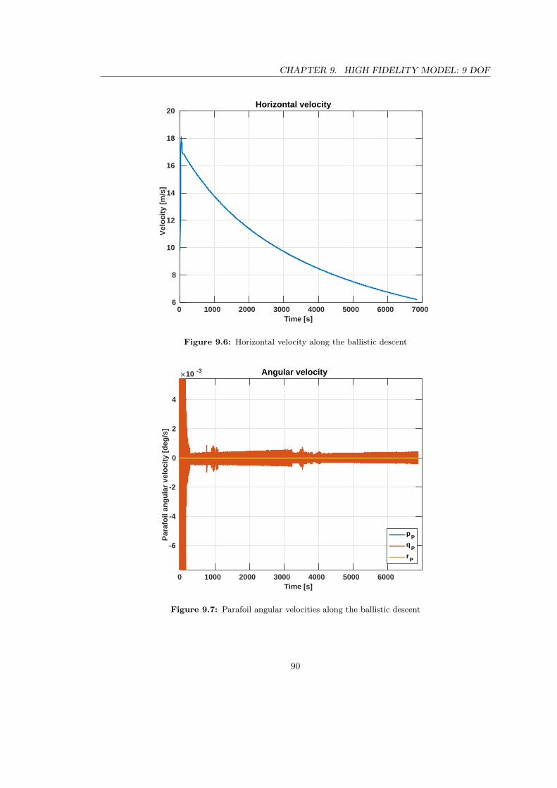
CHAPTER 9. HIGH FIDELITY MODEL: 9 DOF
0 1000 2000 3000 4000 5000 6000 7000Time [s]
6
8
10
12
14
16
18
20
Vel
oci
ty [
m/s
]
Horizontal velocity
Figure 9.6: Horizontal velocity along the ballistic descent
0 1000 2000 3000 4000 5000 6000Time [s]
-6
-4
-2
0
2
4
Par
afo
il an
gu
lar
velo
city
[d
eg/s
]
10 -3 Angular velocity
pP
qP
rP
Figure 9.7: Parafoil angular velocities along the ballistic descent
90

CHAPTER 9. HIGH FIDELITY MODEL: 9 DOF
0 2000 4000 6000 8000Time [s]
-0.08
-0.06
-0.04
-0.02
0
0.02
0.04
0.06
Pay
load
an
gu
lar
velo
city
[d
eg/s
]
Angular velocity
pB
qB
rB
Figure 9.8: Payload angular velocities along the ballistic descent
0 1000 2000 3000 4000 5000 6000 7000Time [s]
-1
-0.8
-0.6
-0.4
-0.2
0
0.2
0.4
0.6
0.8
1
[d
eg]
Roll angle
P
B
Figure 9.9: Roll angle along the ballistic descent
91

CHAPTER 9. HIGH FIDELITY MODEL: 9 DOF
0 1000 2000 3000 4000 5000 6000Time [s]
-4.5
-4
-3.5
-3
-2.5
-2
-1.5
-1
-0.5
[d
eg]
Pitch angle
P
B
Figure 9.10: Pitch angle along the ballistic descent
0 1000 2000 3000 4000 5000 6000 7000Time [s]
-1
-0.8
-0.6
-0.4
-0.2
0
0.2
0.4
0.6
0.8
1
[d
eg]
Yaw angle
P
B
Figure 9.11: Yaw angle along the ballistic descent
92
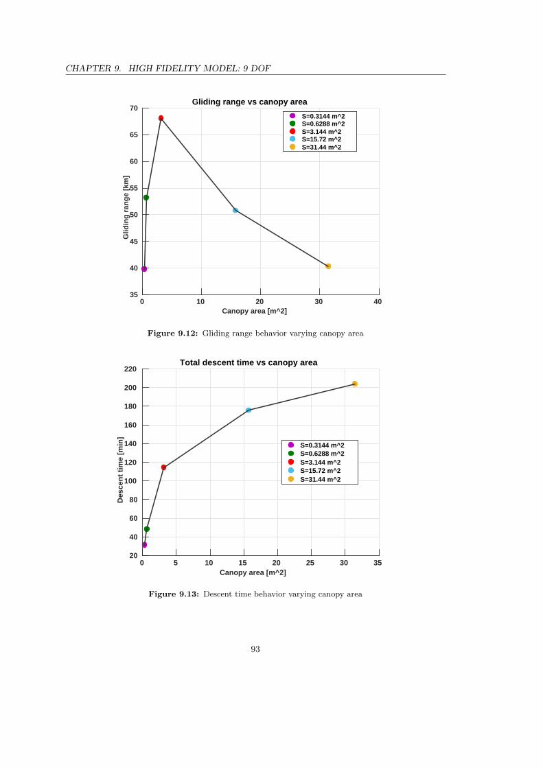
CHAPTER 9. HIGH FIDELITY MODEL: 9 DOF
0 10 20 30 40Canopy area [m^2]
35
40
45
50
55
60
65
70
Glid
ing
ran
ge
[km
]
Gliding range vs canopy area
S=0.3144 m^2S=0.6288 m^2S=3.144 m^2S=15.72 m^2S=31.44 m^2
Figure 9.12: Gliding range behavior varying canopy area
0 5 10 15 20 25 30 35Canopy area [m^2]
20
40
60
80
100
120
140
160
180
200
220
Des
cen
t ti
me
[min
]
Total descent time vs canopy area
S=0.3144 m^2S=0.6288 m^2S=3.144 m^2S=15.72 m^2S=31.44 m^2
Figure 9.13: Descent time behavior varying canopy area
93

CHAPTER 9. HIGH FIDELITY MODEL: 9 DOF
0 10 20 30 40Canopy area [m^2]
5
10
15
20
25
30
35
[d
eg]
Angle of attack vs canopy area
S=0.3144 m^2S=0.6288 m^2S=3.144 m^2S=15.72 m^2S=31.44 m^2
Figure 9.14: Angle of attack behavior varying canopy area
0 10 20 30 40Canopy area [m^2]
2
4
6
8
10
12
14
Vz [
m/s
]
Vertical touchdown velocity vs canopy area
S=0.3144 m^2S=0.6288 m^2S=3.144 m^2S=15.72 m^2S=31.44 m^2
Figure 9.15: Vertical touchdown velocity behavior varying canopy area
94

CHAPTER 9. HIGH FIDELITY MODEL: 9 DOF
0 10 20 30 40Canopy area [m^2]
0
2
4
6
8
10
12
14
Vh
[m
/s]
Horizontal touchdown velocity vs canopy area
S=0.3144 m^2S=0.6288 m^2S=3.144 m^2S=15.72 m^2S=31.44 m^2
Figure 9.16: Horizontal touchdown velocity behavior varying canopy area
0 5 10 15 20 25 30Aspect ratio
-30
-20
-10
0
10
20
30
40
50
60
70
Glid
ing
ran
ge
[km
]
Gliding range vs aspect ratio
AR=0.3AR=0.6AR=3AR=15AR=30
Figure 9.17: Gliding range behavior varying aspect ratio
95

CHAPTER 9. HIGH FIDELITY MODEL: 9 DOF
0 5 10 15 20 25 30Aspect ratio
40
50
60
70
80
90
100
110
120
Des
cen
t ti
me
[min
]
Total descent time vs aspect ratio
AR=0.3AR=0.6AR=3AR=15AR=30
Figure 9.18: Descent time behavior varying aspect ratio
0 5 10 15 20 25 30Aspect ratio
-20
-15
-10
-5
0
5
10
15
20
25
30
[d
eg]
Angle of attack vs aspect ratio
AR=0.3AR=0.6AR=3AR=15AR=30
Figure 9.19: Angle of attack behavior varying aspect ratio
96

CHAPTER 9. HIGH FIDELITY MODEL: 9 DOF
0 5 10 15 20 25 30Aspect ratio
3
4
5
6
7
8
9
10
Vz [
m/s
]
Vertical touchdown velocity vs aspect ratio
AR=0.3AR=0.6AR=3AR=15AR=30
Figure 9.20: Vertical touchdown velocity behavior varying aspect ratio
0 5 10 15 20 25 30Aspect ratio
3.5
4
4.5
5
5.5
6
6.5
Vh
[m
/s]
Horizontal touchdown velocity vs aspect ratio
AR=0.3AR=0.6AR=3AR=15AR=30
Figure 9.21: Horizontal touchdown velocity behavior varying aspect ratio
97

CHAPTER 9. HIGH FIDELITY MODEL: 9 DOF
0 5 10 15 20Line length [m]
45
50
55
60
65
70
75
80
Glid
ing
ran
ge
[km
]
Gliding range vs line length
R=0.1843 mR=0.3686 mR=1.843 mR=9.215 mR=18.43 m
Figure 9.22: Gliding range behavior varying line length
0 5 10 15 20Line length [m]
70
80
90
100
110
120
130
140
Des
cen
t ti
me
[min
]
Total descent time vs line length
R=0.1843 mR=0.3686 mR=1.843 mR=9.215 mR=18.43 m
Figure 9.23: Descent time behavior varying line length
98

CHAPTER 9. HIGH FIDELITY MODEL: 9 DOF
0 5 10 15 20Line length [m]
16
18
20
22
24
26
28
30
32
34
36
[d
eg]
Angle of attack vs line length
R=0.1843 mR=0.3686 mR=1.843 mR=9.215 mR=18.43 m
Figure 9.24: Angle of attack behavior varying line length
0 5 10 15 20Line length [m]
2.5
3
3.5
4
4.5
5
5.5
Vz [
m/s
]
Vertical touchdown velocity vs line length
R=0.1843 mR=0.3686 mR=1.843 mR=9.215 mR=18.43 m
Figure 9.25: Vertical touchdown velocity behavior varying line length
99

CHAPTER 9. HIGH FIDELITY MODEL: 9 DOF
0 5 10 15 20Line length [m]
5.8
5.9
6
6.1
6.2
6.3
6.4
6.5
Vh
[m
/s]
Horizontal touchdown velocity vs line length
R=0.1843 mR=0.3686 mR=1.843 mR=9.215 mR=18.43 m
Figure 9.26: Horizontal touchdown velocity behavior varying line length
-25 -20 -15 -10 -5 0 5 10Rigging angle [deg]
56
58
60
62
64
66
68
70
Glid
ing
ran
ge
[km
]
Gliding range vs rigging angle
=-24 deg=-12 deg=-6 deg=0 deg=6 deg
Figure 9.27: Gliding range behavior varying rigging angle
100

CHAPTER 9. HIGH FIDELITY MODEL: 9 DOF
-25 -20 -15 -10 -5 0 5 10Rigging angle [deg]
90
95
100
105
110
115
120
Des
cen
t ti
me
[min
]
Total descent time vs rigging angle
=-24 deg=-12 deg=-6 deg=0 deg=6 deg
Figure 9.28: Descent time behavior varying rigging angle
-25 -20 -15 -10 -5 0 5 10Rigging angle [deg]
0
5
10
15
20
25
30
[d
eg]
Angle of attack vs rigging angle
=-24 deg=-12 deg=-6 deg=0 deg=6 deg
Figure 9.29: Angle of attack behavior varying rigging angle
101

CHAPTER 9. HIGH FIDELITY MODEL: 9 DOF
-25 -20 -15 -10 -5 0 5 10Rigging angle [deg]
3
4
5
6
7
8
9
Vz [
m/s
]
Vertical touchdown velocity vs rigging angle
=-24 deg=-12 deg=-6 deg=0 deg=6 deg
Figure 9.30: Vertical touchdown velocity behavior varying rigging angle
-25 -20 -15 -10 -5 0 5 10Rigging angle [deg]
4.4
4.6
4.8
5
5.2
5.4
5.6
5.8
6
6.2
6.4
Vh
[m
/s]
Horizontal touchdown velocity vs rigging angle
=-24 deg=-12 deg=-6 deg=0 deg=6 deg
Figure 9.31: Horizontal touchdown velocity behavior varying rigging angle
102

CHAPTER 9. HIGH FIDELITY MODEL: 9 DOF
100 200 300 400 500Payload mass [kg]
67.8
67.85
67.9
67.95
68
68.05
68.1G
lidin
g r
ang
e [k
m]
Gliding range vs payload mass
m=100 kgm=200 kgm=300 kgm=400 kgm=500 kg
Figure 9.32: Gliding range behavior varying payload mass
100 200 300 400 500Payload mass [kg]
70
80
90
100
110
120
130
140
150
160
170
Des
cen
t ti
me
[min
]
Total descent time vs payload mass
m=100 kgm=200 kgm=300 kgm=400 kgm=500 kg
Figure 9.33: Descent time behavior varying payload mass
103
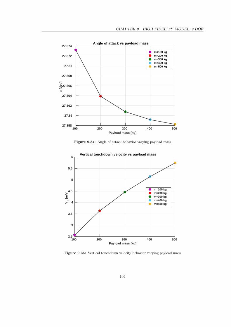
CHAPTER 9. HIGH FIDELITY MODEL: 9 DOF
100 200 300 400 500Payload mass [kg]
27.858
27.86
27.862
27.864
27.866
27.868
27.87
27.872
27.874
[d
eg]
Angle of attack vs payload mass
m=100 kgm=200 kgm=300 kgm=400 kgm=500 kg
Figure 9.34: Angle of attack behavior varying payload mass
100 200 300 400 500Payload mass [kg]
2.5
3
3.5
4
4.5
5
5.5
6
Vz [
m/s
]
Vertical touchdown velocity vs payload mass
m=100 kgm=200 kgm=300 kgm=400 kgm=500 kg
Figure 9.35: Vertical touchdown velocity behavior varying payload mass
104
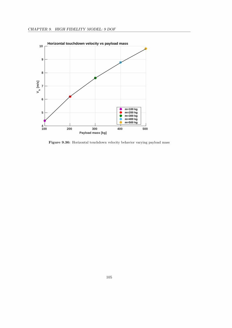
CHAPTER 9. HIGH FIDELITY MODEL: 9 DOF
100 200 300 400 500Payload mass [kg]
4
5
6
7
8
9
10
Vh
[m
/s]
Horizontal touchdown velocity vs payload mass
m=100 kgm=200 kgm=300 kgm=400 kgm=500 kg
Figure 9.36: Horizontal touchdown velocity behavior varying payload mass
105


Chapter 10
Parafoil turn control
In this chapter an algorithm for the parafoil trajectory control will be implemented and usedto simulate different shapes descent (S shape maneuver, spiral maneuver). This procedure hasbeen developed looking to [10]. The implemented method is called Nonlinear Dynamic Inversion(NDI): it is a procedure to access closed-loop characteristic of a system prior to design andtesting a control law. It does not require to linearize the dynamics and it can be used to developclosed-loop system dynamics even at non linear aerodynamic regimes. Thus, NDI is used todesign simple generic non-linear control law for the whole region without detailed analysis. Itis based on the concept of canceling the original dynamic of the system and replacing it withthe desired designed dynamics. States which remain uncontrolled behave according to the open-loop dynamics. This chapter will continue simulating different trajectories using the NDI andinvestigating parafoil turn performances. Finally, parafoil behavior (and the consequent controllogic) in the presence of lateral wind will be analyzed in details.
10.1 NDI applied to parafoil turning
The NDI is used to design a control strategy for parafoil turning. External command variablewhich is necessary to implement this technique is ψP
c, the commanded time story of the yawangle. The objective of this technique is computing the value of δa
d (desired asymmetric deflec-tion) in order to have ψP = ψP
c, keeping δs = 0. The procedure is divided in two steps: first ofall, in an outer loop ψP
c is given in input and the commanded yaw rate rPc is computed; then
the desired asymmetric deflection δad is calculated in an inner loop (giving in input rP
c). Theblock diagram describing the NDI law is presented in Figure 10.1. An assumption which has tobe made (in order to have a good inversion) is that the fast state rP responds much more rapidlythan the slow state ψP . This fact is translated in numbers by the following relation:
ωψωr∼ 0 (10.1)
where ωψ and ωr are bandwidth of ψP and rP . In order to develop the NDI law, the system ofdynamics equations in equation (9.48) have to be rewritten in the form:
Ax = B0 +Bδaδa (10.2)
107

CHAPTER 10. PARAFOIL TURN CONTROL
Figure 10.1: Block diagram of NDI technique
where:
B0 =
B01
B02
B03
B04
(10.3)
B01 = FaB + FgB −ΩBMBΩBrCB (10.4)
B02 = FaP + FgP + FbP −ΩP (MP +MF )ΩP rCP +MFΩPTPVC −ΩPMFTPVC (10.5)
B03 = MgB −ΩBIBωB (10.6)
B04 = Ma0P +MgP +MbP −ΩP IPωP (10.7)
Ma0P =1
2ρVP
2S
b(Clββ +
b
2VPClppP +
b
2VPClrrP )
c(Cm0 + Cmαα+c
2VPCmqqP ) + xpaCz
b(Cnββ +b
2VPCnppP +
b
2VPCnrrP )
(10.8)
Bδa =
000000000
bClδaδa0
bCnδaδa
(10.9)
Basically, the contribution of δa to the right hand side of equations of motion has been isolatedfrom all other terms, in order to be ready for the inversion procedure.
10.1.1 Outer loop inversion
In the outer loop, giving ψPc in input, rP
c is calculated inverting the ψP kinematic equation.
First of all, the commanded parafoil yaw angle is compared with the feedback one getting ψPd
(the desired yaw angle rate) as:˙
ψPd = ωψ(ψP
c − ψP ) (10.10)
108

CHAPTER 10. PARAFOIL TURN CONTROL
Then, inverting the yaw angle dynamics equation (third raw of equation (9.55)) and inserting
ψPd
instead of ψP , the commanded yaw rate can be computed as:
rPc =
ψPd− qP
sin(φP )
cos(θP )
cos(φP )
cos(θP )
(10.11)
It is interesting to note that the outer loop inversion behaves as a first order dynamics systemwith time constant of Tψ = 1/ωψ.
10.1.2 Inner loop inversion
In the inner loop, the desired asymmetric deflection (δad) is calculated giving in input the com-
manded yaw rate (rPc) computed in the outer loop. The commanded and the feedback yaw rate
are compared to compute the desired yaw acceleration as:
˙rPd = ωr(rP
c − rP ) (10.12)
Now the inversion of yaw rate dynamics has to be performed to calculate the desired actuation;yaw rate dynamics equation can be written as:
rP = a(9)(B0 +Bδaδa) (10.13)
where a(9) is a row vector corresponding to the 9th row of matrix A−1 in equation (10.2).
Substituting ˙rP with ˙rPd and inverting the equation, the desired asymmetric deflection can be
computed as:
δad =
˙rPd − a(9)B0
a(9)Bδa(10.14)
During the Matlab simulation, terms a(9)B0 and a(9)Bδa are not computing through A−1 butusing Matlab backslash command which solves linear systems. Also here it is interesting to notethat the inner loop inversion behaves as a first order dynamics system with time constant ofTr = 1/ωr. However in practice, the inner and outer loops couple and the obtained dynamics isnot the exact sum of two first order systems.
10.2 Maneuver simulation with the 9 DOF model
In order to simulate different types of maneuver with the just described control technique, asaturation value of the actuation is inserted in the simulation: this value has been fixed toδmax = 0.1 m, looking to [2, Table 5.3] and remaining a bit conservative. Moreover, sinceequation (10.1) has to be satisfied, values of ωr and ωψ have been fixed keeping a difference oftwo orders of magnitude. Used numbers are: ωr = 100 Hz and ωψ = 1 Hz. An analysis of thebehavior at different bandwidth values will be performed in section 10.2.3. Numerical integrationhas been performed with the ode15s Matlab routine.
10.2.1 S maneuver
The first test of the NDI theory has been done on the 9 DOF system trying to simulate an Sshape maneuver: the ability of performing two turns linked by a rectilinear trajectory has been
109

CHAPTER 10. PARAFOIL TURN CONTROL
proved. This trajectory has been chosen as test because it makes the parafoil completing bigturns spanning the whole angular range (180 degrees in each direction). Hence, the yaw angleinput time history has been set as:
ψP = 0 deg if t < 300 s
ψP = 180 deg if 300 s < t < 2000 s
ψP = 0 deg if t > 2000 s
(10.15)
Results are shown in Figures 10.2, 10.3, 10.4, 10.5, 10.6, 10.7, 10.8, 10.9, 10.10, 10.11, 10.12,10.13 and 10.14; hereafter some important considerations and observations are reported:
• The application of NDI theory works well: the trajectory shape is the expected one.
• α and β values are affected by the actuation and change in time.
• Horizontal and vertical velocity values experience a sudden change due to the actuation;the amount of this effect is bigger if the height is greater, since the density is lower and themaneuver is more effective.
• rP is directly connected to the commanded yaw angle, pP and qP behave by consequence(following their open loop dynamics).
• Payload angular movement depends on the actuation: pB , qB and rB as well as φB , θBand ψB behave according their open loop dynamics.
• ψP time history is the desired one, while θP and φP follow the open loop dynamics; a smalldelay (in yaw angle time evolution) is present due to the system dynamics.
• Actuator saturation is achieved and its effect is to limit the yaw rate to a certain value; byperforming the maneuver at saturation the maximum possible yaw rate is reached.
10.2.2 Spiral maneuver
The second test of NDI capability has been performed simulating a spiral maneuver: this typeof trajectory is useful to stay in proximity of the desired landing site once it has been reachedbut some altitude has to be covered in order to land. The desired actuation is δa = δmax aftertact = 300 s. Results are shown in Figures 10.15, 10.16, 10.17, 10.18, 10.19, 10.20, 10.21, 10.22,10.23, 10.24, 10.25, and 10.26; hereafter some important considerations and observations arereported:
• The spiral trajectory is well simulated; using all parameters defined throughout the entirework (aerodynamic coefficients, geometrical dimensions, bandwidth, actuator saturation)the diameter of the spiral at touchdown is between 550 m and 600 m (this number can bevery useful to start thinking about possible landing sites).
• α and β behavior is affected by the continuous actuation: in particular the angle of sidesliptends to an asymptotic value.
• Vertical velocity increases and horizontal one decreases because of the spiraling trajectory:this type of trajectory is followed to have the maximum possible height loss and to reachplanet surface as soon as possible.
110

CHAPTER 10. PARAFOIL TURN CONTROL
• Speaking about angular velocity, rP tends to an asymptotic value (it is almost constantafter a transient phase), while pP and qP follow the open loop dynamics; consequently, asexpected, ψP increases indefinitely (the parafoil continues to turn) while φP and θP tendto return to zero asymptotically.
• pB and qB oscillate around zero while rB assumes a value slightly different from zero; forthis reason φB and θB varies around zero while ψB increases (but increases less than ψP ).
10.2.3 Tracking capability with different bandwidth values
An analysis on bandwidth values has been carried out. The S shape maneuver described insection 10.2.1 has been simulated in three cases:
• Case 1: ωr = 100 Hz, ωψ = 1 Hz
• Case 2: ωr = 50 Hz, ωψ = 0.5 Hz
• Case 3: ωr = 10 Hz, ωψ = 0.1 Hz
The two orders of magnitude distance between ωr and ωψ have been maintained but their absolutevalues have been varied. Results are shown in Figures 10.27, 10.28 and 10.29. Considerationsthat can be drawn from graphs are:
• Case 3 bandwidth values are too small: the system is not able to follow the commandedyaw rate.
• Case 2 response is slower than Case 1 response; this fact is reasonable since the higher isthe bandwidth the faster is the response.
• Case 1 values are the adopted one.
10.3 Turn performances analysis
Since a tool to perform a controlled turn has been developed and described in previous sections,an analysis on turn performances can be conducted. Performances which have been investigatedare: parafoil maximum turn rate, height loss and total gliding range after a maneuver.
10.3.1 Maximum turn rate
Since a generic turn maneuver is performed varying aerodynamic forces which act on the payload(and therefore it has a dependence on density), the maximum turn rate is function of altitudeabove planet surface. It depends also on the parafoil project parameter δmax, since the turndevelopment in time is function of the amount of actuation given to the parafoil (which cannotbe higher than δmax). As it can be seen from Figure 10.30, the maximum turn rate decreasesas the parafoil approaches the planet (because of density increase) and it is higher for higherδmax. Since the nominal value δmax = 0.1 m has been chosen in a conservative way, this analysishas not been conducted for lower values of δmax, but only for higher ones. The graph reportedin Figure 10.30 has been obtained simulating a descent with δa = δmax from the release to thetouchdown and plotting rP (yaw turn rate) versus altitude. At high altitudes, the maximumturn rate is in the order of 10÷ 20 deg/s while, approaching the planetary surface, it decreasesto values lower than 5 deg/s.
111

CHAPTER 10. PARAFOIL TURN CONTROL
10.3.2 Height loss
The second important performance which has to be analyzed is the height loss due to a maneuver:it is function of altitude and δmax too. It has been investigated using the following technique. Asbefore, a complete descent with δa = δmax has been run and, as expected, the output is a spiralingtrajectory. Results have been discretized every 50 seconds and the difference in height betweentwo consecutive points has been plotted against altitude. The difference in height between twoconsecutive point is the height loss for an hypothetical maneuver at δa = δmax which lasts 50seconds. As it can be seen from Figure 10.31, the height loss due to a maneuver is greater ifthe maneuver itself is performed at an higher altitude. Moreover, as expected, the height lossis greater for a parafoil which has a bigger δmax, since the effect of the deflection has a greaterimpact on parafoil dynamics.
10.3.3 Gliding range
Since a generic maneuver influences parafoil motion in the vertical plane (as it has been explainedin the previous section regarding height loss), the total gliding range is affected by a maneuver.Moreover, the same actuation causes a different effect on the gliding range if it is given to theparafoil at different altitudes. This aspect has been investigated and results are here reported.A maneuver of 150 seconds at maximum deflection has been simulated at different altitudes forδmax = 0.1 m and the consequent variation of the gliding range has been investigated: resultsare shown in Figure 10.32. As it can be seen, the more a maneuver is performed at high altitude,the more the gliding range decreases because of it.
10.4 Parafoil response to a blast of wind
The most relevant external element that can disturb parafoil dynamics is the presence of lateralwind which drifts the system away from the nominal trajectory. This fact can completely jeop-ardize the whole mission, since the landing could occur in an undesired or dangerous location.In order to test the ability of the system to counteract the effect of lateral wind, some analysishave to be performed. The simulation is set in this way: during a ballistic descent, a lateralblast of wind occurs. The wind velocity is defined by the equation (7.1). The lateral blast hasthe effect of changing the trajectory from the nominal one, which is a straight line. The questionto be answered is the following: is there a possibility to come back to the original trajectorycontrolling the parafoil with an asymmetric deflection of lines? First of all, an important hy-pothesis has to be done: all states (positions and velocities) are known, provided somehow by anavigation camera, as if the parafoil is guided by a man. For this particular case, the amountof actuation (in terms of how much left and right lines are pulled) cannot be computed thanksto the NDI technique, since the desired yaw angle time history is not available. The amount ofasymmetric deflection can be directly calculated thanks to a proportional-derivative control lawon the parafoil lateral position and velocity. This sentence is mathematically translated as:
δa(t) = −k1(yc(t)− yd)− k2(vc(t)− vd) (10.16)
where yc(t) and vc(t) are actual lateral position and velocity and yd and vd are desired one.Since the desired trajectory is the ballistic one, yd and vd are set to zero. Gains values have beenchosen as: k1 = 5 ∗ 10−5 and k2 = 1 ∗ 10−2. These numbers have been selected after a trial anderror procedure balancing two needs: avoid as much as possible saturation of the asymmetricactuation and have the response in a reasonable amount of time. Gains values are very small,
112

CHAPTER 10. PARAFOIL TURN CONTROL
since error in terms of position is in the order of hundreds of meters and maximum asymmetricdeflection is 0.1 meters. Two type of wind condition are analyzed:
• First case: after 200 seconds of ballistic descent in zero wind condition, lateral wind appearsand keeps blowing till the touchdown.
• Second case: after 200 seconds of ballistic descent in zero wind condition, lateral windappears; the wind keeps blowing till the descent time reaches 2000 seconds; then, no windcondition takes place till the touchdown.
Results of the simulation in first wind condition are shown in Figures 10.33, 10.34 and 10.35.As it can be seen, the appearance of lateral wind moves the parafoil away from the nominaltrajectory and causes a change in aerodynamic forces produced by the parafoil itself; at thismoment, the parafoil starts pulling the actuation line trying to counteract wind effect, rapidlyreaching saturation condition. After this transient phase (which lasts more or less 80-90 seconds)and when the parafoil acquires again its control capability, the parafoil returns flowing as closeas possible to the nominal trajectory with a value of asymmetric deflection which is differentfrom zero to compensate the on-going lateral wind disturb. As can be observed in graphs, thefinal touchdown lateral position is only a few meters (less than 10) away from the desired one.
Results of the simulation in second wind condition are shown in Figures 10.36, 10.37, 10.38and 10.39. Till 2000 seconds, results are identical to the previous case. A change appears when,2000 seconds after the beginning of the simulation, the lateral wind stops blowing. Since at thismoment the parafoil is flowing with a non zero value of asymmetric actuation, it starts turning,going far away from the nominal trajectory. Also in this case the parafoil needs some time (ahundred of seconds) to produce the necessary amount of deflection to come back to nominal valueof lateral position. The descent continues without any actuation and the landing is reached withthe desired lateral position value.
113
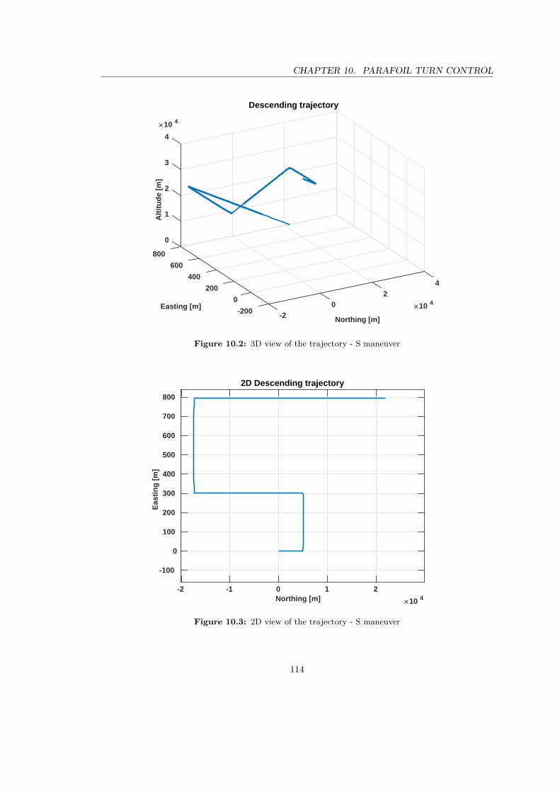
CHAPTER 10. PARAFOIL TURN CONTROL
0
800
1
2
600
Alt
itu
de
[m]
10 4
3
400
Easting [m]
4
Descending trajectory
4
200
Northing [m]
10 42
00
-200 -2
Figure 10.2: 3D view of the trajectory - S maneuver
-2 -1 0 1 2Northing [m] 10 4
-100
0
100
200
300
400
500
600
700
800
Eas
tin
g [
m]
2D Descending trajectory
Figure 10.3: 2D view of the trajectory - S maneuver
114

CHAPTER 10. PARAFOIL TURN CONTROL
0 2000 4000 6000 8000Time [s]
27.5
27.6
27.7
27.8
27.9
28
28.1
28.2 [
deg
]
Angle of attack
Figure 10.4: Angle of attack along the descent - S maneuver
0 1000 2000 3000 4000 5000 6000 7000Time [s]
-5
-4
-3
-2
-1
0
1
2
3
4
[d
eg]
Angle of sideslip
Figure 10.5: Angle of sideslip along the descent - S maneuver
115

CHAPTER 10. PARAFOIL TURN CONTROL
0 1000 2000 3000 4000 5000 6000 7000Time [s]
6
8
10
12
14
16
18
20
Vel
oci
ty [
m/s
]
Horizontal velocity
Figure 10.6: Horizontal velocity along the descent - S maneuver
0 1000 2000 3000 4000 5000 6000 7000Time [s]
2
4
6
8
10
12
14
16
18
20
Vel
oci
ty [
m/s
]
Vertical velocity
Figure 10.7: Vertical velocity along the descent - S maneuver
116

CHAPTER 10. PARAFOIL TURN CONTROL
0 1000 2000 3000 4000 5000 6000 7000Time [s]
-6
-4
-2
0
2
4
6P
araf
oil
ang
ula
r ve
loci
ty [
deg
/s]
Angular velocity
pp
qp
rp
Figure 10.8: Parafoil angular velocities along the descent - S maneuver
0 1000 2000 3000 4000 5000 6000 7000Time [s]
-5
-4
-3
-2
-1
0
1
2
3
4
5
Pay
load
an
gu
lar
velo
city
[d
eg/s
]
Angular velocity
pb
qb
rb
Figure 10.9: Payload angular velocities along the descent - S maneuver
117
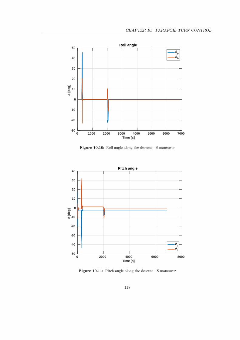
CHAPTER 10. PARAFOIL TURN CONTROL
0 1000 2000 3000 4000 5000 6000 7000Time [s]
-30
-20
-10
0
10
20
30
40
50
[d
eg]
Roll angle
p
b
Figure 10.10: Roll angle along the descent - S maneuver
0 2000 4000 6000 8000Time [s]
-50
-40
-30
-20
-10
0
10
20
30
40
[d
eg]
Pitch angle
p
b
Figure 10.11: Pitch angle along the descent - S maneuver
118
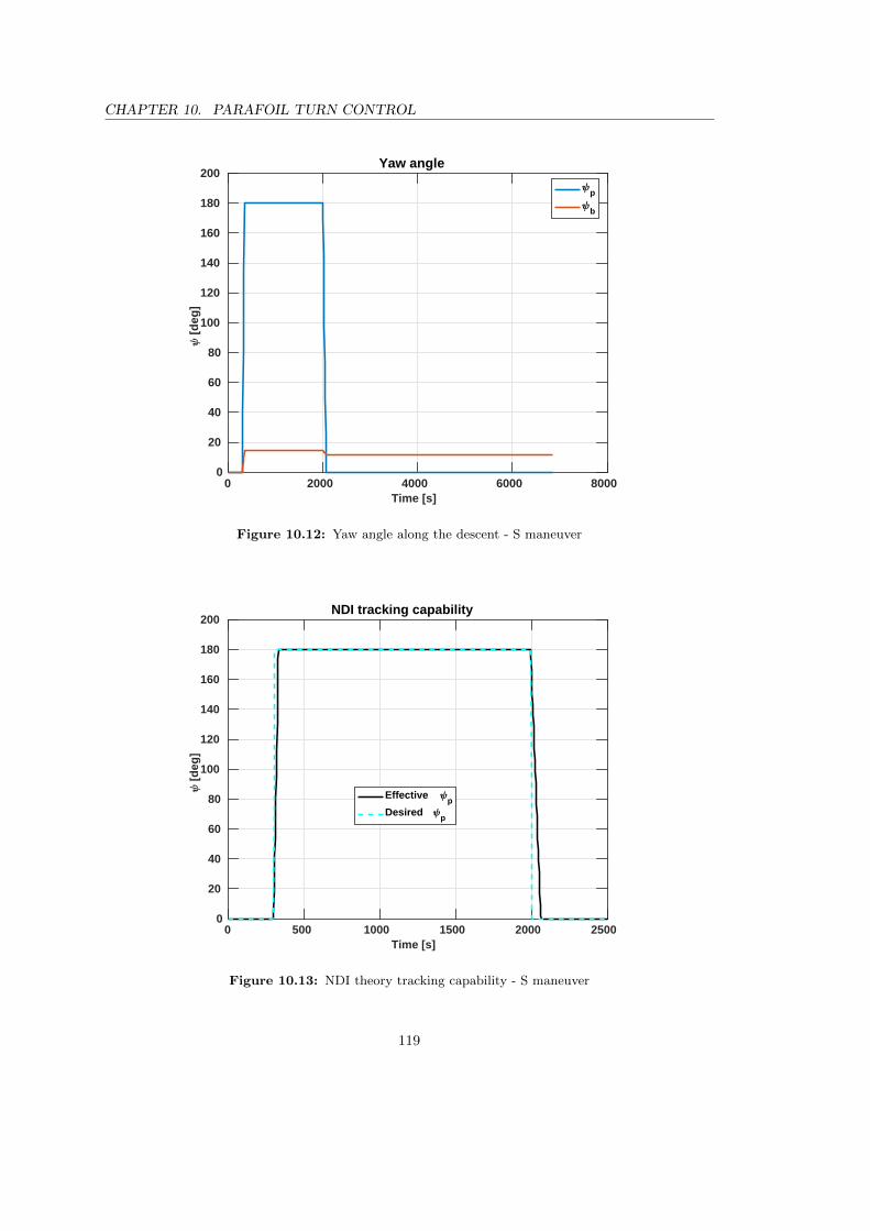
CHAPTER 10. PARAFOIL TURN CONTROL
0 2000 4000 6000 8000Time [s]
0
20
40
60
80
100
120
140
160
180
200
[d
eg]
Yaw angle
p
b
Figure 10.12: Yaw angle along the descent - S maneuver
0 500 1000 1500 2000 2500Time [s]
0
20
40
60
80
100
120
140
160
180
200
[d
eg]
NDI tracking capability
Effective p
Desired p
Figure 10.13: NDI theory tracking capability - S maneuver
119
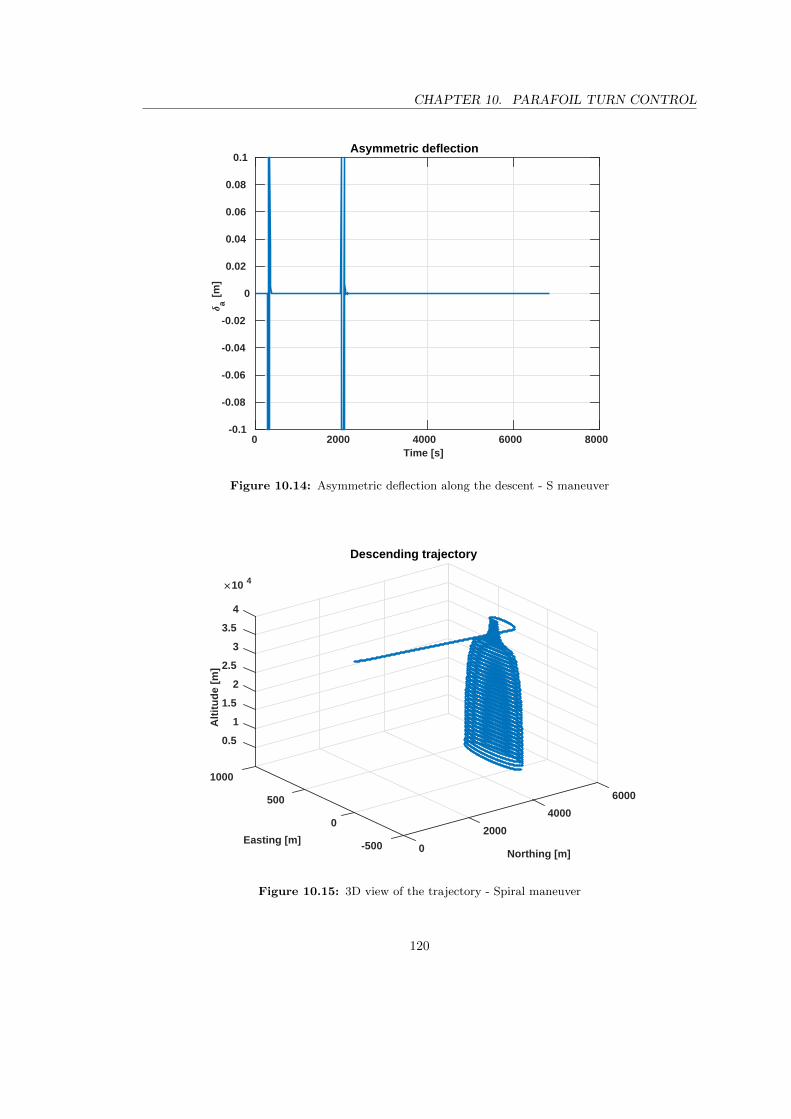
CHAPTER 10. PARAFOIL TURN CONTROL
0 2000 4000 6000 8000Time [s]
-0.1
-0.08
-0.06
-0.04
-0.02
0
0.02
0.04
0.06
0.08
0.1
a [
m]
Asymmetric deflection
Figure 10.14: Asymmetric deflection along the descent - S maneuver
0.5
1000
1
1.5
2
6000
2.5
10 4
Alt
itu
de
[m]
500
3
Descending trajectory
Easting [m]
3.5
4000
Northing [m]
4
02000
-500 0
Figure 10.15: 3D view of the trajectory - Spiral maneuver
120

CHAPTER 10. PARAFOIL TURN CONTROL
4700 4800 4900 5000 5100 5200 5300Northing [m]
0
50
100
150
200
250
300
350
400
450
500E
asti
ng
[m
]
2D Descending trajectory
Figure 10.16: 2D view of the trajectory (zoom) - Spiral maneuver
0 1000 2000 3000 4000 5000 6000Time [s]
27.6
27.65
27.7
27.75
27.8
27.85
27.9
[d
eg]
Angle of attack
Figure 10.17: Angle of attack along the descent - Spiral maneuver
121

CHAPTER 10. PARAFOIL TURN CONTROL
0 1000 2000 3000 4000 5000 6000 7000Time [s]
-6
-5
-4
-3
-2
-1
0
1
[d
eg]
Angle of sideslip
Figure 10.18: Angle of sideslip along the descent - Spiral maneuver
0 1000 2000 3000 4000 5000 6000 7000Time [s]
6
8
10
12
14
16
18
20
Vel
oci
ty [
m/s
]
Horizontal velocity
Figure 10.19: Horizontal velocity along the descent - Spiral maneuver
122

CHAPTER 10. PARAFOIL TURN CONTROL
0 1000 2000 3000 4000 5000 6000 7000Time [s]
0
5
10
15
20
25
Vel
oci
ty [
m/s
]
Vertical velocity
Figure 10.20: Vertical velocity along the descent - Spiral maneuver
0 1000 2000 3000 4000 5000 6000Time [s]
-6
-4
-2
0
2
4
6
8
10
12
14
Par
afo
il an
gu
lar
velo
city
[d
eg/s
]
Angular velocity
pp
qp
rp
Figure 10.21: Parafoil angular velocities along the descent - Spiral maneuver
123

CHAPTER 10. PARAFOIL TURN CONTROL
0 1000 2000 3000 4000 5000 6000Time [s]
-10
-5
0
5
10
Pay
load
an
gu
lar
velo
city
[d
eg/s
]
Angular velocity
pb
qb
rb
Figure 10.22: Payload angular velocities along the descent - Spiral maneuver
0 1000 2000 3000 4000 5000 6000 7000Time [s]
-40
-30
-20
-10
0
10
20
30
40
50
[d
eg]
Roll angle
p
b
Figure 10.23: Roll angle along the descent - Spiral maneuver
124

CHAPTER 10. PARAFOIL TURN CONTROL
0 1000 2000 3000 4000 5000 6000 7000Time [s]
-60
-50
-40
-30
-20
-10
0
10
20
30
40
[d
eg]
Pitch angle
p
b
Figure 10.24: Pitch angle along the descent - Spiral maneuver
0 1000 2000 3000 4000 5000 6000 7000Time [s]
0
5000
10000
15000
[d
eg]
Yaw angle
p
b
Figure 10.25: Yaw angle along the descent - Spiral maneuver
125

CHAPTER 10. PARAFOIL TURN CONTROL
0 1000 2000 3000 4000 5000 6000 7000Time [s]
0
0.01
0.02
0.03
0.04
0.05
0.06
0.07
0.08
0.09
0.1
a [
m]
Asymmetric deflection
Figure 10.26: Asymmetric deflection along the descent - Spiral maneuver
-2 -1 0 1 2
Northing [m] 104
-100
0
100
200
300
400
500
600
700
800
900
Ea
sti
ng
[m
]
In-plane descending trajectory
r=100 Hz, =1 Hz
r=50 Hz, =0.5 Hz
r=10 Hz, =0.1 Hz
Figure 10.27: 2D view of the trajectory with different bandwidth values
126

CHAPTER 10. PARAFOIL TURN CONTROL
0 500 1000 1500 2000 2500
Time [s]
-50
0
50
100
150
200
250
[d
eg
]
Yaw angle time evolution
r=100 Hz, =1 Hz
r=50 Hz, =0.5 Hz
r=10 Hz, =0.1 Hz
Desired
Figure 10.28: Yaw angle behavior with different bandwidth values
290 295 300 305 310Time [s]
-5
0
5
10
15
20
[d
eg]
Yaw angle time evolution - zoom
r=100 Hz, =1 Hz
r=50 Hz, =0.5 Hz
r=10 Hz, =0.1 Hz
Desired
Figure 10.29: Zoom of yaw angle behavior with different bandwidth values
127

CHAPTER 10. PARAFOIL TURN CONTROL
0 5 10 15 20 25Turn rate [deg/s]
0
5
10
15
20
25
30
35
40
Hei
gh
t [k
m]
Maximum turn rate variation with altitude
max=0.1 m
max=0.15 m
max=0.2 m
max=0.25 m
Figure 10.30: Maximum turn rate variation with altitude for different δmax values
0 200 400 600 800 1000 1200 1400
Height loss [m]
0
5
10
15
20
25
30
35
40
Heig
ht
[km
]
Maneuver height loss variation with altitude
max=0.1 m
max=0.15 m
max=0.2 m
max=0.25 m
Figure 10.31: Maneuver height loss variation with altitude for different δmax values
128

CHAPTER 10. PARAFOIL TURN CONTROL
6.3 6.4 6.5 6.6 6.7
Gliding range [m] 10 4
0
5
10
15
20
25
30
35
40
He
igh
t [k
m]
Gliding range vs maneuver altitude
max=0.1
Figure 10.32: Gliding range variation with altitude at which the maneuver is performed
0 1 2 3 4 5 6 7x [m] 10 4
-20
0
20
40
60
80
100
120
140
y [m
]
2D trajectory
Figure 10.33: 2D view of the trajectory after first type of lateral blast of wind
129

CHAPTER 10. PARAFOIL TURN CONTROL
0 1000 2000 3000 4000 5000 6000 7000Time [s]
-0.1
-0.08
-0.06
-0.04
-0.02
0
0.02
0.04
a [
m]
Asymmetric deflection
Figure 10.34: Asymmetric deflection after first type of lateral blast of wind
0 200 400 600 800Time [s]
-0.1
-0.08
-0.06
-0.04
-0.02
0
0.02
a [
m]
Asymmetric deflection
Figure 10.35: Zoom of asymmetric deflection after first type of lateral blast of wind
130

CHAPTER 10. PARAFOIL TURN CONTROL
0 1 2 3 4 5 6 7x [m] 10 4
-100
-50
0
50
100
150y
[m]
2D trajectory
Figure 10.36: 2D view of the trajectory after second type of lateral blast of wind
0 1000 2000 3000 4000 5000 6000 7000Time [s]
-0.1
-0.08
-0.06
-0.04
-0.02
0
0.02
0.04
0.06
a [
m]
Asymmetric deflection
Figure 10.37: Asymmetric deflection after second type of lateral blast of wind
131

CHAPTER 10. PARAFOIL TURN CONTROL
0 100 200 300 400 500 600 700Time [s]
-0.1
-0.08
-0.06
-0.04
-0.02
0
0.02
a [
m]
Asymmetric deflection
Figure 10.38: First zoom of asymmetric deflection after second type of lateral blast of wind
1600 1800 2000 2200 2400 2600Time [s]
0
0.01
0.02
0.03
0.04
0.05
a [
m]
Asymmetric deflection
Figure 10.39: Second zoom of asymmetric deflection after second type of lateral blast of wind
132

Chapter 11
Actuation implementation
In this chapter the derivation and the implementation of a dynamical model representing theway thanks to which line deflection occurs will be described. First of all, the focus will be on thecalculation of the moment acting on the system because of the actuation itself and of the tensionin actuation line. After that, a dynamical model of the electric motor through which actuationreally happens will be derived and then applied to the system, performing a comparison betweenideal case (chapter 10) and real one.
11.1 Torque acting on the system, line tension and re-quested power
To have a better understanding of the actuation procedure, left and right command (δl and δr)instead of asymmetric one (δa) have to be computed. They are defined as:
If δa > 0 −→
δl = δa
δr = 0(11.1)
If δa < 0 −→
δl = 0
δr = −δa(11.2)
The moment acting on the whole system because of an actuation is embedded in the aerodynamicmoment expression in equation (9.33). It is basically the part of Ma which is function of δa. Itsexpression as function of δr and δl is:
τsp = QSb
Clδa −Clδa0 0
Cnδa −Cnδa
[δrδl
](11.3)
This is the value of the torque acting on the system because of an actuation written in parafoilreference frame. With the just written relation, values of δl and δr (and consequently δa) requiredto perform a maneuver with a desired τsp can be computed. This expression enlarges the numberof ways in which amount of actuation can be computed and it adds robustness to the parafoilcontrol logic.
Then, tension in actuation lines have to be computed. The following derivation is performedfor the right actuation; necessary changing for the tension in left line will be underlined later.
133

CHAPTER 11. ACTUATION IMPLEMENTATION
Figure 11.1: Schematic view of actua-tion line triangle if δa = 0
Figure 11.2: Schematic view of actua-tion line triangle if δa 6= 0
The followed approach is a geometric one; canopy deformation because of an actuation is notconsidered. Pulley is supposed to be put at line conjunction, so at point C of Figure 9.1. Lookingto Figure 11.1 the following relation can be easily written:
d2 =
√|RP |2 +
b
2
2
(11.4)
On the contrary, looking to Figure 11.2, following relation can be retrieved (using the law ofcosines for a generic triangle):
β1 = cos−1
((d2 − δr)2 − |RP |2 −
b
2
2
|RP |b
2
)(11.5)
Once these quantities have been computed, the vector which represents the actuation line (mag-nitude, direction and versus) in the parafoil reference frame can be written as:
d2p =
−|RP | sin(µ)b
2sin(β1)
−|RP | cos(µ) +b
2cos(β1)
(11.6)
At this point an assumption about the position of the center of mass of the entire system hasto be done. Since the payload is much heavier than the parafoil, the system center of mass issupposed to be at payload center. Vector which represents the distance between center of massand point C (in payload reference frame) is:
dCMb =
00
−|RB |
(11.7)
134
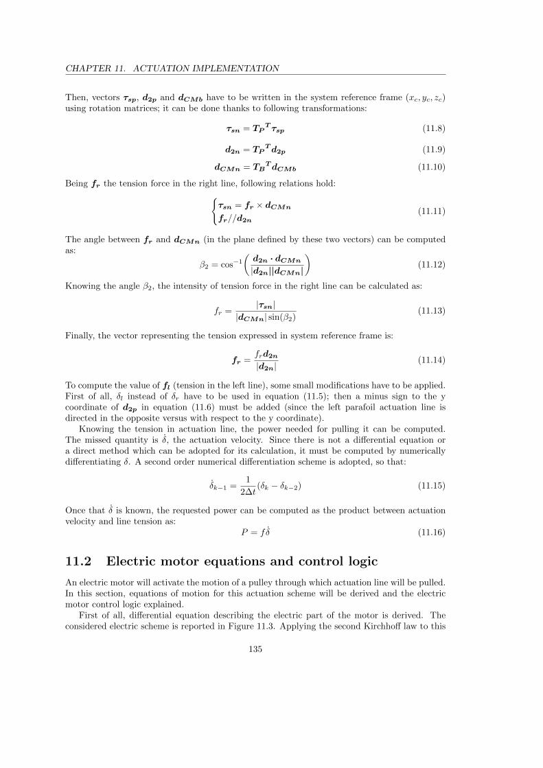
CHAPTER 11. ACTUATION IMPLEMENTATION
Then, vectors τsp, d2p and dCMb have to be written in the system reference frame (xc, yc, zc)using rotation matrices; it can be done thanks to following transformations:
τsn = TPT τsp (11.8)
d2n = TPTd2p (11.9)
dCMn = TBTdCMb (11.10)
Being fr the tension force in the right line, following relations hold:τsn = fr × dCMn
fr//d2n(11.11)
The angle between fr and dCMn (in the plane defined by these two vectors) can be computedas:
β2 = cos−1
(d2n · dCMn
|d2n||dCMn|
)(11.12)
Knowing the angle β2, the intensity of tension force in the right line can be calculated as:
fr =|τsn|
|dCMn| sin(β2)(11.13)
Finally, the vector representing the tension expressed in system reference frame is:
fr =frd2n|d2n|
(11.14)
To compute the value of fl (tension in the left line), some small modifications have to be applied.First of all, δl instead of δr have to be used in equation (11.5); then a minus sign to the ycoordinate of d2p in equation (11.6) must be added (since the left parafoil actuation line isdirected in the opposite versus with respect to the y coordinate).
Knowing the tension in actuation line, the power needed for pulling it can be computed.The missed quantity is δ, the actuation velocity. Since there is not a differential equation ora direct method which can be adopted for its calculation, it must be computed by numericallydifferentiating δ. A second order numerical differentiation scheme is adopted, so that:
δk−1 =1
2∆t(δk − δk−2) (11.15)
Once that δ is known, the requested power can be computed as the product between actuationvelocity and line tension as:
P = f δ (11.16)
11.2 Electric motor equations and control logic
An electric motor will activate the motion of a pulley through which actuation line will be pulled.In this section, equations of motion for this actuation scheme will be derived and the electricmotor control logic explained.
First of all, differential equation describing the electric part of the motor is derived. Theconsidered electric scheme is reported in Figure 11.3. Applying the second Kirchhoff law to this
135

CHAPTER 11. ACTUATION IMPLEMENTATION
Figure 11.3: Circuit describing the electricalpart of the motor
Figure 11.4: Scheme describing the mechan-ical part of the motor
circuit, the following equation can be written:
Lai+Rai− eb = ea (11.17)
where i is the current intensity flowing in the circuit, La and Ra are inductance and resistanceof the electric motor, ea is the voltage given by the battery and eb is the voltage delivered to themechanical part of the motor. On the contrary, looking to the mechanical part of the motor andreferring to Figure 11.4, the following differential equation can be written:
− Cm + Jθ + cθ +Rmf = 0 (11.18)
where θ is the variable describing pulley angular position, f is line tension modulus, Rm is pulleyradius, J is the inertia (the motor one plus the pulley one), c is the damping coefficient and Cm isthe torque acting on the pulley due to the presence of the motor. There are two relations whichlink mechanical and electrical part of the system. They come from the consideration that, fromthe electromechanical point of view, the motor transforms power (from electric to mechanicalone) without generating or dissipating it. This implies that eb and Cm can be written as functionof the same function k (called motor characteristic) as:
eb = −kω (11.19)
Cm = ki (11.20)
Defining current intensity (i), pulley angular position (θpulley) and pulley angular velocity (ωpulley)as state variables and combining equations (11.17), (11.18), (11.19) and (11.20), equations of mo-tion of the electric motor system can be written as:
i =ea − kωpulley −Rai
La
ωpulley =−Rmf + ki+ cωpulley
J
θpulley = ωpulley
(11.21)
Since the value of desired asymmetric deflection is known (as explained in chapter 10), a controllogic for the motor can be implemented: in this way pulley angular position will assume the
136

CHAPTER 11. ACTUATION IMPLEMENTATION
Figure 11.5: Block diagram of electric motor control logic
value such that the associated asymmetric deflection will be as close as possible to the desiredone. The motor is controlled varying value of supply voltage ea. Knowing the desired angularposition of the pulley, the supply voltage (which is the control variable) can assume the followingform:
ea = Kcontrol(θdesired − θpulley) (11.22)
where Kcontrol is the proportional control gain. The desired angular position θdesired can becalculated knowing the desired line deflection and the pulley radius as:
θdesired =δ
Rm(11.23)
assuming that θpulley = 0 when δ = 0. One point has to be made: here a generic symbol δ hasbeen used to define the line deflection, no matter of left or right line. Clearly, the system willhave two identical electric motor with two pulley: derivation of equations of motion is the samefor them and δ is δr or δl depending on which line is considered.
Furthermore, an explanation of the whole control logic can be done. A block scheme de-scribing it is presented in Figure 11.5. The desired δa is computed as explained in chapter 10;then, left and right desired deflection can be computed according to equations (11.1) and (11.2).After that, desired left and right pulley position can be calculated using (11.23) and the controlvariable ea is computed thanks to equation (11.22). Then, after the integration of equations ofmotion of the motor (equation (11.21)), the effective left and right actuation can be recomputedas function of the real pulley position as:
δeff = θpulleyRm (11.24)
Also here δ is the generic symbol; this equation have to be implemented for both left andright line. Finally, knowing left and right effective actuation, the effective δa can be calculatedinverting equation (11.1) and (11.2). This is the value of control variable which enters the parafoilequations of motion.
11.3 Simulations
Simulations of maneuvers described in chapter 10 have been performed with the insertion ofelectric motor equations and control logic just described; results will be here reported. Usedelectric motor parameters are summarized in Table 11.1. What must be underlined is that amaximum value for the supply tension have been fixed and that pulley radius has been chosenso that the maximum line shortening of 0.1 m can be wrap around it. For each case, values ofmaximum requested power and maximum tension line will be given: these numbers will be usefulto start sizing components (the physical actuation line, the pulley and the electric motor itself).Value of maximum line tension will always be almost the same, since it depends on maximumpossible deflection value which has been fixed to δmax = 0.1 m.
137
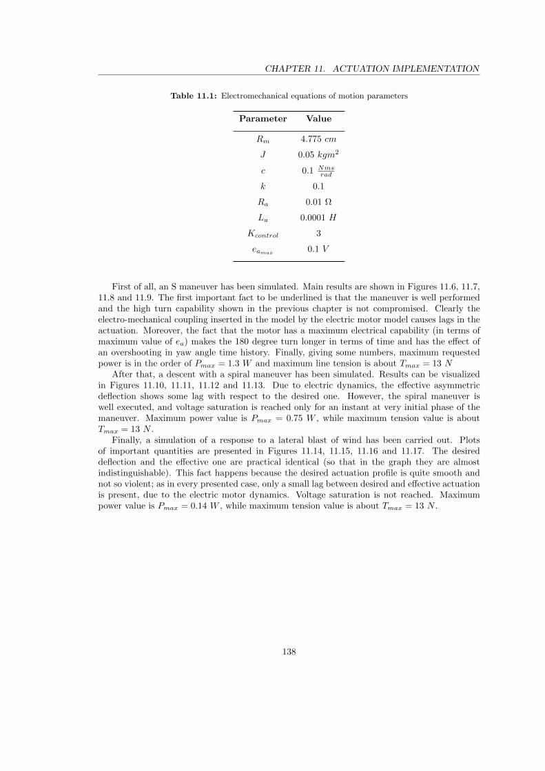
CHAPTER 11. ACTUATION IMPLEMENTATION
Table 11.1: Electromechanical equations of motion parameters
Parameter Value
Rm 4.775 cm
J 0.05 kgm2
c 0.1 Nmsrad
k 0.1
Ra 0.01 Ω
La 0.0001 H
Kcontrol 3
eamax 0.1 V
First of all, an S maneuver has been simulated. Main results are shown in Figures 11.6, 11.7,11.8 and 11.9. The first important fact to be underlined is that the maneuver is well performedand the high turn capability shown in the previous chapter is not compromised. Clearly theelectro-mechanical coupling inserted in the model by the electric motor model causes lags in theactuation. Moreover, the fact that the motor has a maximum electrical capability (in terms ofmaximum value of ea) makes the 180 degree turn longer in terms of time and has the effect ofan overshooting in yaw angle time history. Finally, giving some numbers, maximum requestedpower is in the order of Pmax = 1.3 W and maximum line tension is about Tmax = 13 N
After that, a descent with a spiral maneuver has been simulated. Results can be visualizedin Figures 11.10, 11.11, 11.12 and 11.13. Due to electric dynamics, the effective asymmetricdeflection shows some lag with respect to the desired one. However, the spiral maneuver iswell executed, and voltage saturation is reached only for an instant at very initial phase of themaneuver. Maximum power value is Pmax = 0.75 W , while maximum tension value is aboutTmax = 13 N .
Finally, a simulation of a response to a lateral blast of wind has been carried out. Plotsof important quantities are presented in Figures 11.14, 11.15, 11.16 and 11.17. The desireddeflection and the effective one are practical identical (so that in the graph they are almostindistinguishable). This fact happens because the desired actuation profile is quite smooth andnot so violent; as in every presented case, only a small lag between desired and effective actuationis present, due to the electric motor dynamics. Voltage saturation is not reached. Maximumpower value is Pmax = 0.14 W , while maximum tension value is about Tmax = 13 N .
138

CHAPTER 11. ACTUATION IMPLEMENTATION
0 1000 2000 3000 4000 5000 6000 7000Time [s]
-0.1
-0.08
-0.06
-0.04
-0.02
0
0.02
0.04
0.06
0.08
0.1a
[m
]
Asymmetric deflection
a desired
a effective
Figure 11.6: Desired and effective asymmetric deflection - S maneuver
0 1000 2000 3000 4000 5000 6000 7000Time [s]
0
2
4
6
8
10
12
14
Fo
rce
[N]
Line tension
fl
fr
Figure 11.7: Left and right line tension - S maneuver
139

CHAPTER 11. ACTUATION IMPLEMENTATION
0 2000 4000 6000 8000Time [s]
-0.1
-0.08
-0.06
-0.04
-0.02
0
0.02
0.04
0.06
0.08
0.1
Vo
ltag
e [V
]
Required voltage
eal
ear
Figure 11.8: Left and right required voltage - S maneuver
0 1000 2000 3000 4000 5000 6000 7000Time [s]
0
0.2
0.4
0.6
0.8
1
1.2
1.4
P [
W]
Requested power for the actuation
Pl
Pr
Figure 11.9: Left and right requested power - S maneuver
140

CHAPTER 11. ACTUATION IMPLEMENTATION
0 1000 2000 3000 4000 5000 6000 7000Time [s]
0
0.01
0.02
0.03
0.04
0.05
0.06
0.07
0.08
0.09
0.1
a [
m]
Asymmetric deflection
a desired
a effective
Figure 11.10: Desired and effective asymmetric deflection - Spiral maneuver
0 1000 2000 3000 4000 5000 6000 7000Time [s]
0
2
4
6
8
10
12
14
Fo
rce
[N]
Line tension
f l
f r
Figure 11.11: Left and right line tension - Spiral maneuver
141

CHAPTER 11. ACTUATION IMPLEMENTATION
0 1000 2000 3000 4000 5000 6000 7000Time [s]
0
0.01
0.02
0.03
0.04
0.05
0.06
0.07
0.08
0.09
0.1
Vo
ltag
e [V
]
Required voltage
eal
ear
Figure 11.12: Left and right required voltage - Spiral maneuver
0 1000 2000 3000 4000 5000 6000 7000Time [s]
0
0.1
0.2
0.3
0.4
0.5
0.6
0.7
0.8
P [
W]
Requested power for the actuation
P l
P r
Figure 11.13: Left and right requested power - Spiral maneuver
142

CHAPTER 11. ACTUATION IMPLEMENTATION
0 1000 2000 3000 4000 5000 6000 7000Time [s]
-0.1
-0.08
-0.06
-0.04
-0.02
0
0.02
0.04
0.06a
[m
]
Asymmetric deflection
a desired
a effective
Figure 11.14: Desired and effective asymmetric deflection for a response to a blast of wind
0 1000 2000 3000 4000 5000 6000 7000Time [s]
0
2
4
6
8
10
12
14
Fo
rce
[N]
Line tension
fl
fr
Figure 11.15: Left and right line tension for a response to a blast of wind
143

CHAPTER 11. ACTUATION IMPLEMENTATION
0 1000 2000 3000 4000 5000 6000 7000Time [s]
-0.02
0
0.02
0.04
0.06
0.08
0.1
Vo
ltag
e [V
]
Required voltage
eal
ear
Figure 11.16: Left and right required voltage for a response to a blast of wind
0 1000 2000 3000 4000 5000 6000 7000Time [s]
0
0.02
0.04
0.06
0.08
0.1
0.12
0.14
P [
W]
Requested power for the actuation
P l
P r
Figure 11.17: Left and right requested power for a response to a blast of wind
144

Chapter 12
Payload attitude control
The motion of the entire system will take place in a real environment with possible presence ofdisturbances (gust wind); in order to maintain the payload as still as possible, a payload attitudecontrol logic has been studied and inserted in the model. Actuators presence implies the use ofa set of sensors and filters. Sensors, actuators and disturbances modeling as well as results ofsimulations will be discussed in this chapter.
12.1 Gust wind model
The wind has a deterministic component (described in section 7.1) and a stochastic one: inliterature it is called gust wind. The presence of this wind component has to be implementedin the model: it is a disturbance for the payload attitude. It has been firstly modeled in acontinuous way and then in a discrete one according to [14].
12.1.1 Continuous approach
The stochastic model for the wind is based on a first order Markov model. Is is assumed thatthe varying wind can be represented by the following differential equation:
v(t) = −βv(t) + σnw(t) (12.1)
where v(t) is the wind velocity and w(t) is a generic random process whose variance is σn.Solution of equation (12.1) involves transition matrix Φ in the form:
Φ(∆t) = e−β∆t (12.2)
But the desired form of wind differential equation is the following one:
x(t) = F (t)x(t) +G(t)ω(t) (12.3)
where ω(t) is a zero mean, unity variance white noise. Comparing equations (12.1) and (12.3)it is possible to get that: v(t) = x(t), −β = F (t) and σn = G(t). The covariance of state x(t)
is defined as X(t) = E[(x(t)− x(t))2], where x(t) is the mean value of variable x(t) and the
operator E[ ] is the expected value. Evolution in time of the state covariance written in matrixform is obtained from equation (12.3) as:
X(t) = F (t)X(t) +X(t)F (t)T
+G(t)Q(t)G(t) (12.4)
145

CHAPTER 12. PAYLOAD ATTITUDE CONTROL
where Q(t) is the white noise process covariance. But, since the problem is completely scalar,setting Q(t) = q = 1, equation (12.4) can be written as:
X(t) = −2βX(t) + σn2 (12.5)
Solution of this first order differential equation is:
X(t) =σn2β
(1− e2βt) (12.6)
assuming X(t = 0) = 0 as initial condition. As it is possible to see, the process is stationary; infact X(t) tents to a finite value as t approaches infinite:
limt→∞
X(t) =σn
2
2β(12.7)
But, since X(t) = E[(v(t)− ¯v(t))2], also the following relation holds:
limt→∞
X(t) = σv2 (12.8)
Combining equations (12.7) and (12.8), the following relation can be easily retrieved:
σn =√
2βσv (12.9)
This is the necessary scaling factor for the white noise process that has to be taken into accountin order to simulate the phenomenon in the right way.
12.1.2 Discrete approximation
The use of a continuous differential equation (equation (12.1)) for the wind noise model producessignificant computational trashing. The reason behind this fact is that, numerically speaking, thewhite noise process has to be approximated by calling a Gaussian random white noise generator.This means that the right hand side of equation (12.1) does not reproduce always the same valueas t approaches a specific instant tk, because two sampling of ω(tk) do not produce the samevalue. Therefore, the wind speed model has to be computed a priori in a discrete way. Equation(12.1) has to be converted in a discrete time step version:
xk+1 = Φ(∆t)xk + ξk (12.10)
where ξk is the contribution of the white noise process over the time interval; it can be computedaccording to the following equation:
ξk =
∫ tk+1
tk
Φ(tk+1 − t)σnω(t) dt (12.11)
Unfortunately, the real white noise ω(t) is not accessible; the only available quantity is a randomlygenerated number ωk, which is the sampling of the white noise between tk and tk+1 (∆t =tk+1 − tk). The question to be answered now is: how can this number be scaled over the timeinterval in order to approximate the effect of the true white noise ω(t)? The quantity ξk has tobe written as function of ωk:
ξk =√E[ξk]2ωk (12.12)
146

CHAPTER 12. PAYLOAD ATTITUDE CONTROL
Applying the definition of expected value to the square of equation (12.11) the expected valueof ξk
2 can be computed as:
E[ξk]2 =
∫ tk+1
tk
Φ2(tk+1 − t)σn2E[(ω(t)− ω(t))2] dt (12.13)
But a white noise process has unit variance; so:
E[(ω(t)− ω(t))2] = 1 (12.14)
Applying the change of variable τ = tk+1 − t to integral in equation (12.13), E[ξk]2 turns out tobe:
E[ξk]2 = σn2
∫ ∆t
0
Φ(τ)2dτ (12.15)
Remembering equation (12.2), this integral can be written as:
E[ξk]2 = σn2
∫ ∆t
0
e−2βτ dτ = −σn2
2β(e−2β∆t − 1) (12.16)
Since ∆t is small, (e−2β∆t − 1) ∼ (−2β∆t). Therefore:
E[ξk]2 = −σn2
2β(−2β∆t) = σn
2∆t (12.17)
Recalling equation (12.12), ξk can be written as:
ξk =√E[ξk]2ωk =
√σn2∆tωk = σn
√∆tωk (12.18)
Thanks to the just developed procedure, equation (12.10) can be transformed in a usable formas (remembering equation (12.2) for the transition matrix):
xk+1 = e−β∆txk + σn√
∆tωk (12.19)
Using equation (12.9) and saying that (e−β∆t) ∼ (1−β∆t) since ∆t is small, the discrete updateequation for the gust wind model becomes:
xk+1 = xk − β∆txk + (√
2β∆tσv)ωk (12.20)
The gust wind model is computed before the integration with this discrete equation; at eachintegration step the effective gust wind will be calculated with a first order interpolation ofpoints sequence created with equation (12.20).
12.1.3 Stochastic parameters variation with height
In order to be able to insert the gust wind model in the whole simulation, values of wind velocitystandard deviation (σv) and of wind auto correlation time (Tv) have to be estimated. Thecorrelation time is an important parameter to be defined, since β = 1/Tv. In theory they canbe retrieved applying statistics formulae to an appropriate set of measured data; this procedureis explained in [14]. Unfortunately, an appropriate set of high frequency Titan wind measures isnot available: for this reason, σv and Tv values have to be estimated in another way, retrievingdata from literature.
147

CHAPTER 12. PAYLOAD ATTITUDE CONTROL
0 1000 2000 3000 4000 5000 6000 7000Time [s]
-2.5
-2
-1.5
-1
-0.5
0
0.5
1
1.5
2
2.5
Win
d [
m/s
]
Example of gust wind model
Figure 12.1: Gust wind in x direction for the reference height of 36000 m
A turbulent wind model (developed for earth atmosphere) is presented in [13, cha. 10.3.3]:from this work, data for the Titan gust wind model have been estimated. Terrestrial model dataare relative to correlation length (Lcorr) and turbulence standard deviation (σv). The correlationlength is always fixed to the value Lcorr = 150 m, while the turbulence standard deviation is set toσv = 0.6m/s at h = 40000m, σv = 0.8m/s at h = 10000m and σv = 0.9m/s at h = 1000m (themedium profile is taken into account). Auto correlation time is then computed as Tv = Lcorr/V ,where V is the parafoil velocity in the right direction. Since standard deviation varies with height,and also auto correlation time does (since velocities change during the descent), a turbulent windmodel variable with height has to be implemented. But the gust wind model, as explained in theprevious section, has to be generated a priori with a discrete time scheme before the integration(and not with a discrete height scheme). The adopted solution is to take five reference altitudebetween release and touchdown, compute σv and Tv at this altitude (σv is calculated with a linearinterpolation on available data while Tv is calculated taking from a reference ballistic descentvalues for velocities at different altitudes), generate the gust wind model and then, during thesimulation, select the right gust wind model according to the altitude at which the parafoil is.
Another point has to be underlined: since parafoil vertical and horizontal velocities aredifferent, also Tv relative to gust wind in vertical and horizontal directions will not be equal.They will be calculated as:
Tvz =LcorrVh
(12.21)
Tvh =LcorrVz
(12.22)
Tvz will be used to generate the gust wind profile in z direction, while Tvh for x and y direction.As example, gust wind in x direction for the reference height of 36000 m is reported in Figure12.1. In Table 12.1 values used to generate five turbulent wind models at five reference altitudesare reported.
148
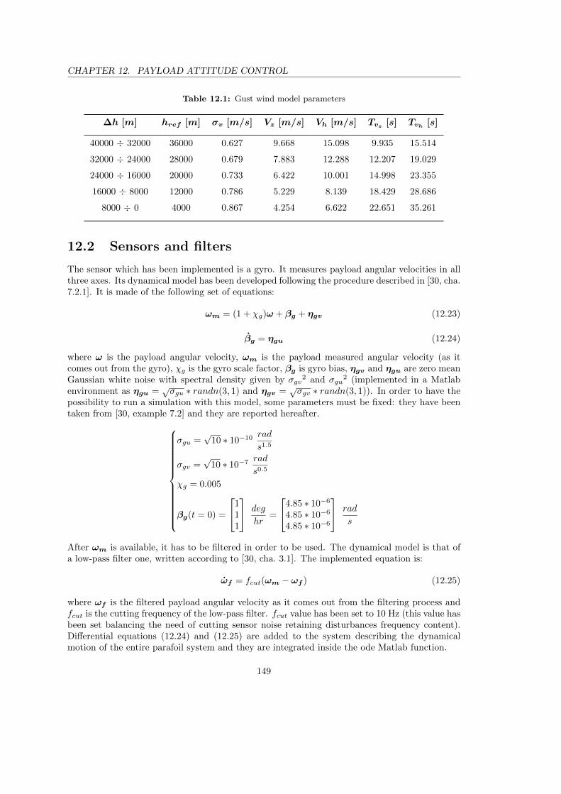
CHAPTER 12. PAYLOAD ATTITUDE CONTROL
Table 12.1: Gust wind model parameters
∆h [m] href [m] σv [m/s] Vz [m/s] Vh [m/s] Tvz [s] Tvh [s]
40000 ÷ 32000 36000 0.627 9.668 15.098 9.935 15.514
32000 ÷ 24000 28000 0.679 7.883 12.288 12.207 19.029
24000 ÷ 16000 20000 0.733 6.422 10.001 14.998 23.355
16000 ÷ 8000 12000 0.786 5.229 8.139 18.429 28.686
8000 ÷ 0 4000 0.867 4.254 6.622 22.651 35.261
12.2 Sensors and filters
The sensor which has been implemented is a gyro. It measures payload angular velocities in allthree axes. Its dynamical model has been developed following the procedure described in [30, cha.7.2.1]. It is made of the following set of equations:
ωm = (1 + χg)ω + βg + ηgv (12.23)
βg = ηgu (12.24)
where ω is the payload angular velocity, ωm is the payload measured angular velocity (as itcomes out from the gyro), χg is the gyro scale factor, βg is gyro bias, ηgv and ηgu are zero meanGaussian white noise with spectral density given by σgv
2 and σgu2 (implemented in a Matlab
environment as ηgu =√σgu ∗ randn(3, 1) and ηgv =
√σgv ∗ randn(3, 1)). In order to have the
possibility to run a simulation with this model, some parameters must be fixed: they have beentaken from [30, example 7.2] and they are reported hereafter.
σgu =√
10 ∗ 10−10 rad
s1.5
σgv =√
10 ∗ 10−7 rad
s0.5
χg = 0.005
βg(t = 0) =
111
deg
hr=
4.85 ∗ 10−6
4.85 ∗ 10−6
4.85 ∗ 10−6
rad
s
After ωm is available, it has to be filtered in order to be used. The dynamical model is that ofa low-pass filter one, written according to [30, cha. 3.1]. The implemented equation is:
ωf = fcut(ωm − ωf ) (12.25)
where ωf is the filtered payload angular velocity as it comes out from the filtering process andfcut is the cutting frequency of the low-pass filter. fcut value has been set to 10 Hz (this value hasbeen set balancing the need of cutting sensor noise retaining disturbances frequency content).Differential equations (12.24) and (12.25) are added to the system describing the dynamicalmotion of the entire parafoil system and they are integrated inside the ode Matlab function.
149

CHAPTER 12. PAYLOAD ATTITUDE CONTROL
12.3 Camera
A camera (which will be used for navigation purpose) has to be put on the bottom surface ofthe payload. In order to be the most general possible, camera position has been chosen not incorrespondence of joint C and of payload center, but away from this point. Precisely:
Pcam =
PxcamPycamPzcam
=
0.1250.1250.75
m (12.26)
is the vector between joint C and camera position. The aim of the following procedure is tocalculate the relative displacement between joint C and camera, converting it then in αx andαy, angles which describe the camera pointing vector time evolution. vc vector (velocity ofpoint C) is known inside the integration procedure: it is part of state vector; the same can besaid for rc, joint position vector. Three more variables are added to the state vector: they arercam = [xcam, ycam, zcam]′, and they describe the motion of the camera point. A differentialequation thanks to which rcam evolution in time can be computed is necessary. To accomplishthis goal, velocity vector of the camera point vcam shall be calculated. It can be computed usingrigid body kinematics relation as:
vcam = vc + ωb ×
xc − xcamyc − ycamzc − zcam
(12.27)
Then, the vector rcam time evolution is ruled by the following differential equation:
rcam = vcam (12.28)
Relative displacement between junction and camera can be computed as:
∆x = xcam − xc − Pxcam (12.29)
∆y = ycam − yc − Pycam (12.30)
∆z = zcam − zc − Pzcam (12.31)
Camera point angles (αx and αy) can be calculated as:
αx = 2 sin−1
(∆x/2√
Pxcam2 + Pzcam
2
)(12.32)
αy = 2 sin−1
(∆y/2√
Pycam2 + Pzcam
2
)(12.33)
In order to give the possibility to the camera of acquiring images of the planetary surface, αx andαy variation shall stay in the order of milliradians. The matching of this pointing requirementhas been used to evaluate the goodness of different actuators schemes.
150
CHAPTER 12. PAYLOAD ATTITUDE CONTROL
12.4 Simulation without attitude control
First of all, effects of gust wind on payload attitude control have to be investigated: a ballisticdescent without any type of attitude control has been carried out. Results are shown in Figures12.4 and 12.5. As can be seen, the gust wind causes a variation of the pointing angle in the orderof 10 deg (αx goes from −10 deg to 8 deg and αx from −7 deg to 7 deg) and angular velocitiesassume values up to 5 deg/s. The conclusion that can be drawn from this analysis is that apayload attitude control scheme is necessary to give to th camera the possibility of acquiringimages. The aim of following sections is to reduce these values, trying to stabilize the payloadexploiting different attitude control solutions. One important thing must be underlined: thenumerical integration has been performed with a Runge-Kutta 4 method (RK4) and not withthe always used ode15s Matlab routine (and the same has been done for all simulations presentedin this chapter). This is due to the fact that the introduction of white noise generator avoids theuse of a variable step integration scheme (as ode15s) since the simulation becomes too slow.
12.5 First control attempt: reaction wheels as actuators
The first attempt for controlling payload attitude is done using three reaction wheels (RW) asactuators. They can deliver a variable control torque to the payload exchanging their momentum,linearly linked to the wheel angular velocity. First of all, reaction wheels modeling process willbe described; then, after the definition of the control law, results of a simulation with reactionwheels, sensors, filters and wind disturbance as just described will be presented.
12.5.1 Reaction wheels modeling
The reaction wheels dynamics modeling is described in following passages; it has been developedaccording to [34, cha. 6]. Up to now, payload rotational equation of motion (section 9.1) can bewritten in a compact way as:
JωB = τB − ωB × JωB (12.34)
where τB is the sum of all moments acting on the payload, J is payload inertia matrix and ωBis payload angular velocity. But now equations of motion has to be rewritten, considering thepresence of three reaction wheels. Angular momentum of the payload and of the reaction wheelcan be written as:
hB = JωB (12.35)
hw = Jw(ωw + ωB) (12.36)
where hw, Jw and ωw are respectively angular momentum, inertia and angular velocity of thereaction wheel. Equations of motion of the system ”payload + wheels” can be written exploitingthe equality between angular momentum variation and total moment acting on the system.Specifically they can be written for the payload and the reaction wheel as:
H = τB (12.37)
hw = τw (12.38)
where H = hB + hw is the angular momentum of the whole system. Combining equations(12.35), (12.36), (12.37) and (12.38), equations of motion of payload and wheel can be writtenrespectively as:
JωB + JwωB + Jwωw + ωB × ((J + Jw)ωB + Jwωw) = τB (12.39)
151

CHAPTER 12. PAYLOAD ATTITUDE CONTROL
Jw(ωw + ωB) = τw (12.40)
The term τw is the control moment; it will be defined in a following section (according to thepayload desired attitude behavior). Matrix Jw is defined as:
Jw =
Iw 0 00 Iw 00 0 Iw
(12.41)
where Iw = mwR2w is the inertia of a single wheel (mw is the mass of the wheel and Rw is its
radius). In order to write Jw according to equation (12.41), an hypothesis has to be made: thethree reaction wheels are oriented towards three orthogonal directions which are principle axes ofinertia. Comparing equations (12.39) and (12.40) with equations of motion of the system withoutreaction wheels (equation (9.48)), equations of motion of the system composed by parafoil,payload and reaction wheels can be written as Ax = B, where:
A =
−MBSrCB 03x3 MBTB TB 03x3
03x3 −(MP +MF )SrCP (MP +MF )TP −TP 03x3
IB + Jw 03x3 03x3 −SrCBTB Jw03x3 IP + IF 03x3 SrCP TP 03x3
Jw 03x3 03x3 03x3 Jw
(12.42)
x =
ωBωPVCFCωw
(12.43)
B =
B1
B2
B3
B4
B5
(12.44)
B1 = FaB + FgB −ΩBMBΩBrCB (12.45)
B2 = FaP +FgP +FbP −ΩP (MP +MF )ΩP rCP +MFΩPTPVC−ΩPMFTPVC (12.46)
B3 = MgB −ΩBIBωB − ωB × (JwωB + Jwωw) (12.47)
B4 = MaP +MgP +MbP −ΩP IPωP (12.48)
B5 = τw (12.49)
A final observation has to be made: a reaction wheel has not an infinite capability. For thisreason, physical constrains (in terms of maximum torque (τmax) and maximum momentum(hmax)) have to be added to the model. They are inserted thanks to following equations
− τmax < τw < τmax (12.50)
− hmax < Jwωw < hmax (12.51)
Saturation limits have been set to
τmax =
0.40.40.4
Nm (12.52)
152

CHAPTER 12. PAYLOAD ATTITUDE CONTROL
and
hmax =
100100100
Nms (12.53)
These numbers have been chosen in accordance to [31], taking the HR16 model as a reference.Also the value for Iw can be computed looking to the same datasheet as:
Iw = mwR2w = 2.096 kgm2 (12.54)
12.5.2 Control law definition
In order to control payload attitude with three reaction wheels in presence of disturbances, asuitable control law has to be implemented. The chosen control logic is a PD feedback law forpointing, which tries to bring to zero Euler angle error and angular velocity one. It is defined as:
τd =
c1(pB − pd)c2(qB − qd)c3(rB − rd)
+
k1(φB − φd)k2(θB − θd)k3(ψB − ψd)
(12.55)
where ω = [pB , qB , rB ]′ is the payload angular velocity vector as it comes out from the filter,θ = [φB , θB , ψB ]′ is the payload angular position vector (since inserting a measuring model forEuler angles is very difficult, θ is not the measured angular position vector, but it is the real one),ωd = [pd, qd, rd]
′ and θd = [φd, θd, ψd]′ are desired values for angular positions and velocities and
c = [c1, c2, c3]′ and k = [k1, k2, k3]′ are gains. Numbers used in the simulation are:
c1 = 0.5
c2 = 0.1
c3 = 0.5
k1 = 0.5
k2 = 0.1
k3 = 0.5
φd = 0 rad
θd = −0.0366 rad
ψd = 0 rad
pd = 0rad
s
qd = 0rad
s
rd = 0rad
s
The value of θd has been chosen in this way because it is the equilibrium value. During a ballisticdescent without any disturbance, the payload flies at a pitch angle different from zero and almostequal to −2.1 deg = −0.0366 rad (this angle slightly varies with time, −2.1 deg has been takenas average value).
153
CHAPTER 12. PAYLOAD ATTITUDE CONTROL
12.5.3 Simulation results
Results of the simulation of a ballistic descent with reaction wheels control and wind disturbancesare shown in Figures 12.6, 12.7 and 12.8. As it can be seen, the gust wind disturbance has a toohigh frequency content and too high value to give the possibility to reaction wheels to completelycontrol payload attitude matching the requirement of keeping camera pointing angles variationin the order of milliradians. Moreover, reaction wheels dynamics couples with payload attitudeone causing the opposite effect: camera pointing angles assume higher values with respect to theballistic case (their variation is in the order of dozens of degrees). Payload angular velocitiesincreases along the descent reaching values up to 12 deg/s. Possible solution to have a betterattitude control can be the exploitation of different attitude actuators.
12.6 Second control attempt: ideal control
As explained in previous section, reaction wheels are not capable to provide a suitable control,since gust wind has a too high frequency content and too high maximum value. The aim of thissection of the work is to understand which is the torque that have to be given to the payload tokeep camera pointing error in the order of milliradians and payload angular velocities in the orderof 10 milliradians in presence of gust wind, no matter of the type of actuation. Basically, the aimis the calculation of the ideal control torque needed to completely fulfill pointing requirements.
The control torque is computed thanks to a proportional derivative feedback law, as justdescribed in section (12.5.2). Its expression is here reported for completeness.
Mc = −
k1(φB − φd) + c1(pB − pd)k2(θB − θd) + c2(qB − qd)k3(ψB − ψd) + c3(rB − rd)
(12.56)
The term Mc is added to equations of motion as an external torque applied to the payload,without any dynamics (contrary to reaction wheels, whose control process passes through theirdynamics). It is merely summed to B3 in equation (9.51), which becomes:
B3 = MgB −ΩBIBωB +Mc (12.57)
Values of gains have been selected after a trial and error procedure, finally choosing the lowestvalues of them which gives the possibility to satisfy requirements. Since position and velocityrequirements are very demanding, these numbers are much higher than the ones used in thesimulation with reaction wheels. They have been chosen as:
k1 = 18000
k2 = 12000
k3 = 1000
c1 = 18000
c2 = 12000
c3 = 1000
Results of the simulation with the presence of gust wind and with an ideal control are shown inFigures 12.9, 12.10 and 12.11 . Important numerical results are hereafter reported. Maximum
154

CHAPTER 12. PAYLOAD ATTITUDE CONTROL
Figure 12.2: 16 thrusters configuration
camera pointing errors (in terms of maximum and minimum values of αx and αy) are:
αx −→
+0.13 deg = +2.27 mrad
−0.08 deg = −1.40 mrad(12.58)
αy −→
+0.12 deg = +2.09 mrad
−0.07 deg = −1.22 mrad(12.59)
These maximum values are sporadically reached during the whole simulation, while for most ofthe time angles values are smaller: looking to Figure 12.9, it can be seen that camera pointingrequirements are satisfied, since αx and αy assume a value in the order of milliradians all thesimulation long. Moreover, maximum payload angular velocities are:
ωB −→
+0.15 deg
s = +2.62 mrads
−0.15 degs = −2.62 mrad
s
(12.60)
These values are reached by roll and pitch angular rate and not by the yaw one. The require-ment of keeping payload angular velocities in the order of 10 milliradians is completely satisfied.Finally, maximum values of requested control torque have to be analyzed; they are:
τd −→
+30 Nm
−30 Nm(12.61)
This pick value of 30 Nm is sometimes reached by the control torque in roll angular direction.Values of angular position and velocity accuracy and of needed torque are clearly related toselected gust wind parameters and to payload and parafoil dimensions: changing them, requestedtorque and effective angular position and velocity can change. However, the developed simulationframework can serve as a tool to this type of analysis; moreover, considerations about reactionwheels uselessness and about other actuation type are still valid.
12.6.1 Hints on possible types of attitude actuators
How can this control moment be delivered to the payload? A suitable actuators set has to beselected. Since analysis about this mission concept are at an early stage, no solutions on how the
155

CHAPTER 12. PAYLOAD ATTITUDE CONTROL
Figure 12.3: Thrusters selection for each type of rotation
payload attitude can be controlled have been proposed yet. Some ideas (and relative drawbacks)are hereafter reported.
As shown before, reaction wheels are not capable to adequately control the payload, becausetheir maximum torque delivered is far from 30 Nm and their dynamics is too slow to follow thegust wind high frequency variation.
The first proposed possible solution is to use a certain number of thrusters. For example, the20 N thruster from datasheet [32] can be an appropriate choice. If this solution will be adopted,a certain number of tanks inside the payload will have to be allocated. A drawback relativeto the implementation of a thruster solution can be the value of Minimum Impulse Bit of thethruster itself. Since the gust wind is a highly varying disturb, the fact that the thruster is notcapable to deliver a continuous thrust (which, on the contrary, is constituted by a series of smallconstant intervals of thrust) can become problematic. The smaller the Minimum Impulse Bit ofthe thruster is, the easier will be to precisely deliver the desired control moment to the payload.A first idea on how thrusters can be spatially organized on the payload is given in Figure 12.2,where orange arrows represent thrust direction of each small engine; moreover, Figure 12.3 showshow positive and negative rotations about each axis can be performed.
The second proposed solution is the insertion of Control Moment Gyros as attitude controlactuators. As can be seen in datasheet [33], CMGs are able to deliver a control torque in theorder of 30 Nm (in this case it is up to 45 Nm). The issue related to this type of actuators isrelated to their dimensions and their weight: they are big and heavy and, for this reason, it couldbe difficult to find space for them inside the payload and to integrate them in the system.
The final possible solution for attitude payload control is the insertion of a viscoelastic jointable to damp the box movement at the connection between payload and parafoil. The feasibilityof this idea will be probably studied in the future.
156
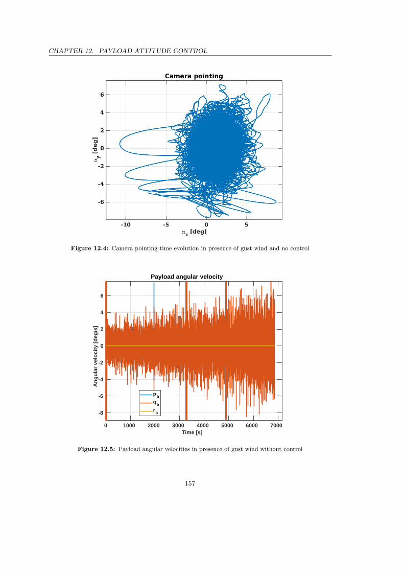
CHAPTER 12. PAYLOAD ATTITUDE CONTROL
Figure 12.4: Camera pointing time evolution in presence of gust wind and no control
0 1000 2000 3000 4000 5000 6000 7000Time [s]
-8
-6
-4
-2
0
2
4
6
An
gu
lar
velo
city
[d
eg/s
]
Payload angular velocity
pb
qb
rb
Figure 12.5: Payload angular velocities in presence of gust wind without control
157

CHAPTER 12. PAYLOAD ATTITUDE CONTROL
Figure 12.6: Camera pointing time evolution in presence of gust wind and reaction wheels control
0 1000 2000 3000 4000 5000 6000 7000
Time [s]
-15
-10
-5
0
5
10
15
An
gu
lar
velo
cit
y [
deg
/s]
Payload angular velocity
pb
qb
rb
Figure 12.7: Payload angular velocities in presence of gust wind and reaction wheels control
158

CHAPTER 12. PAYLOAD ATTITUDE CONTROL
0 1000 2000 3000 4000 5000 6000 7000Time [s]
-0.4
-0.3
-0.2
-0.1
0
0.1
0.2
0.3
0.4
To
rqu
e [N
*m]
RW control torque
p control torqueq control torquer control torque
Figure 12.8: Reaction wheels control torque in presence of gust wind
Figure 12.9: Camera pointing with an ideal control torque
159

CHAPTER 12. PAYLOAD ATTITUDE CONTROL
1000 2000 3000 4000 5000 6000 7000Time [s]
-0.2
-0.15
-0.1
-0.05
0
0.05
0.1
0.15
0.2
An
gu
lar
velo
city
[d
eg/s
]
Payload angular velocity
pb
qb
rb
Figure 12.10: Payload angular velocities with an ideal control torque
0 1000 2000 3000 4000 5000 6000Time [s]
-30
-20
-10
0
10
20
30
To
rqu
e [N
*m]
Control torque
p control torqueq control torquer control torque
Figure 12.11: Ideal control torque
160

Chapter 13
Atmospheric parametersestimation
Along the chapter, methods for the real time estimation of atmospheric parameters which influ-ence parafoil descent (wind field and atmospheric density) will be described. The goodness ofthese procedures will be shown thanks to error analysis and simulations. The wind field proce-dure relies on a direct computation, while the density estimator has the structure of an extendedKalman filer.
13.1 Wind field estimation
Knowledge of the wind field is generally implicitly assumed in UAV and parafoil research. Thissection tries to find an answer to the following question: is there a possibility to perform a quiteeasy wind field estimation using sensing that is already available on-board? An important facthas to be underlined: accurate measurements of wind field (including spatial gradient) can beobtained using arrays of multi-hole pitot probes (according to [27]). This procedure is out ofthe purpose of the work, since this instruments set is not usually on-board on parafoils. Set ofmeasurements that are assumed available to perform the wind estimation is made of:
• Ground speed
• Parafoil state (position, orientation and velocity with respect to the airmass)
These data cannot come from GPS (since it is not available on Titan) and have to be wellestimated or computed knowing the state of the orbiter which communicates with the parafoilcomputer. However, the availability of these measurements is assumed, but the fact that acalculation or estimation procedure is behind their accessibility have to be underlined.
First of all, the wind field estimation procedure will be explained; then, an analysis of esti-mation procedure error will be performed; finally the effectiveness of the procedure will be testedwith a Monte Carlo simulation and the procedure will be used to produce a forward estimation(based on least square minimization process) of the lateral wind the parafoil will encounter alongthe descent. The whole discussion has been developed according to [28].
161
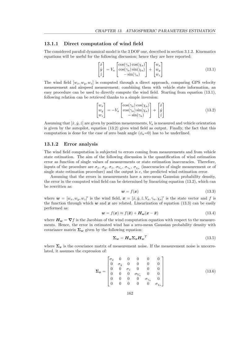
CHAPTER 13. ATMOSPHERIC PARAMETERS ESTIMATION
13.1.1 Direct computation of wind field
The considered parafoil dynamical model is the 3 DOF one, described in section 3.1.2. Kinematicsequations will be useful for the following discussion; hence they are here reported:xy
z
= Va
cos(γa) cos(χa)cos(γa) sin(χa)− sin(γa)
+
wxwywz
(13.1)
The wind field [wx, wy, wz] is computed through a direct approach, comparing GPS velocitymeasurement and airspeed measurement; combining them with vehicle state information, aneasy procedure can be used to directly compute the wind field. Starting from equation (13.1),following relation can be retrieved thanks to a simple inversion:wxwy
wz
= −Va
cos(γa) cos(χa)cos(γa) sin(χa)− sin(γa)
+
xyz
(13.2)
Assuming that [x, y, z] are given by position measurements, Va is measured and vehicle orientationis given by the autopilot, equation (13.2) gives wind field as output. Finally, the fact that thiscomputation is done for the case of zero bank angle (φa=0) has to be underlined.
13.1.2 Error analysis
The wind field computation is subjected to errors coming from measurements and from vehiclestate estimation. The aim of the following discussion is the quantification of wind estimationerror as function of single values of measurements or state estimation inaccuracies. Therefore,inputs of the procedure are σx, σy, σz, σVa , σγa , σχa (inaccuracies of single measurement or ofsingle state estimation procedure) and the output is e, the predicted wind estimation error.
Assuming that the errors in measurements have a zero-mean Gaussian probability density,the error in the computed wind field can be determined by linearizing equation (13.2), which canbe rewritten as:
w = f(x) (13.3)
where w = [wx, wy, wz]′ is the wind field, x = [x, y, z, Va, γa, χa]′ is the state vector and f is
the function through which w and x are related. Linearization of equation (13.3) can be easilyperformed as:
w = f(x) ≈ f(x) +Hw(x− x) (13.4)
where Hw =∇f is the Jacobian of the wind computation equation with respect to the measure-ments. Hence, the error in estimated wind has a zero-mean Gaussian probability density withcovariance matrix Σw given by the following equation:
Σw = HwΣxHwT (13.5)
where Σx is the covariance matrix of measurement noise. If the measurement noise is uncorre-lated, it assumes the expression of:
Σx =
σx 0 0 0 0 00 σy 0 0 0 00 0 σz 0 0 00 0 0 σVa 0 00 0 0 0 σγa 00 0 0 0 0 σχa
(13.6)
162

CHAPTER 13. ATMOSPHERIC PARAMETERS ESTIMATION
The Jacobian of w with respect to measurements and states is obtained looking to equation(13.2); its expression is:
Hw =
1 0 0 − cos(γa) cos(χa) Va sin(γa) cos(χa) Va cos(γa) sin(χa)0 1 0 − cos(γa) sin(χa) Va sin(γa) sin(χa) −Va cos(γa) cos(χa)0 0 1 sin(γa) Va cos(γa) 0
(13.7)
Performing matrix product shown in equation (13.5), Σw terms assume the following form:
Σw(1, 1) = σx2 + σVa
2 cos2(γa) cos2(χa)+
+ σγa2Va
2 sin2(γa) cos2(χa) + σχa2Va
2 cos2(γa) sin2(χa) (13.8)
Σw(2, 2) = σy2 + σVa
2 cos2(γa) sin2(χa)+
+ σγa2Va
2 sin2(γa) sin2(χa) + σχa2Va
2 cos2(γa) cos2(χa) (13.9)
Σw(3, 3) = σz2 + σVa
2 sin2(γa) + σγa2Va
2 cos2(γa) (13.10)
Σw(1, 2) = Σw(2, 1) = (sin(χa) cos(χa))(σVa2cos2(γa)+
+ σγa2Va
2sin2(γa)− σχa2Va2cos2(γa)) (13.11)
Σw(1, 3) = Σw(3, 1) = (cos(γa) sin(γa) cos(χa))(−σVa2 + σγa2Va
2) (13.12)
Σw(2, 3) = Σw(3, 2) = (cos(γa) sin(γa) sin(χa))(−σVa2 + σγa2Va
2) (13.13)
The error covariance matrix is symmetric. Off-diagonal terms of covariance matrix Σw repre-sent correlation between estimated wind component. In particular, terms Σw(1, 3) and Σw(2, 3)are related to the correlation between vertical and horizontal wind components: it can be re-moved if these terms are zero. Equations (13.12) and (13.13) lead to the consideration thatcorrelation between horizontal and vertical wind components can be removed by flying at γa = 0(horizontally with respect to the air mass). This is possible only with a powered flight (out of theparafoil framework), since a steady glide will always result in the parafoil descending in relationto the surrounding air mass. Going forward, term Σw(1, 2) represents the correlation betweenthe two horizontal wind components. Also in this case, it can be removed nullifying term inequation (13.11). Hence, it is possible to remove correlation between the two horizontal windcomponent by flying at χa = 0 deg, 90 deg, 180 deg, 270 deg. In practice, noise in measurementswill be correlated, but this fact will not affect the error estimation.
Indeed, a good measure of the total error in wind estimation procedure is the trace of thecovariance matrix Σw. It can be calculates as:
e2 = Tr(Σw) = Σw(1, 1) + Σw(2, 2) + Σw(3, 3) =
= σx2 + σy
2 + σz2+
+σVa2(cos2(γa)cos2(χa) + cos2(γa)sin2(χa) + sin2(γa))+
+σγa2Va
2(sin2(γa)cos2(χa) + sin2(γa)sin2(χa) + cos2(γa))+
+σχa2Va
2(cos2(γa)sin2(χa) + cos2(γa)cos2(χa)) = (13.14)
= σx2 + σy
2 + σz2 + σVa
2(cos2(γa)(cos2(χa) + sin2(χa)) + sin2(γa))+
+σγa2Va
2(sin(γa)2(cos2(χa) + sin2(χa)) + cos2(γa))+
+σχa2Va
2(cos2(γa)(sin2(χa) + cos2(χa))) =
= σx2 + σy
2 + σz2 + σVa
2 + Va2(σγa
2 + σχa2cos2(γa))
163

CHAPTER 13. ATMOSPHERIC PARAMETERS ESTIMATION
Table 13.1: Measurement noise and estimate uncertainties for simulations
Parameter Source Uncertainty
Orientation State estimate from autopilot σχa = σγa = 1 deg
Ground speed Position measurement via autopilot σx = σy = σz = 0.1 ms
Air speed State estimate from autopilot σVa = 0.2 ms
As can be seen, the error in wind estimation procedure depends on both single measurementsor autopilot estimation errors and flight condition (Va and γa). The prediction of the expressionjust written is that the error will be higher for a greater value of airspeed. In a simulation, thepredicted wind estimation error given by equation (13.14) can be compared with the real one.
13.1.3 Monte Carlo simulation
To assess the feasibility of the proposed estimation scheme, a Monte Carlo simulation has beenconducted, investigating the effectiveness of wind estimation procedure and comparing the realerror with the predicted one. Under the condition defined in Table 13.1, whose values have beentaken from [28], the expected error in wind velocity estimation assumes the form:
e2 = 0.07 + Va2(0.0003(1 + cos2(γa))) (13.15)
Measured quantities, which will be used to perform wind estimation, are calculated startingfrom real ones adding a normally distributed random number (pxm , pym , pzm , pVa , pγa , pχa)adequately scaled according to the uncertainty associated to each of them:
xm = x+ σxpxm (13.16)
ym = y + σypym (13.17)
zm = z + σzpzm (13.18)
Vam = Va + σVapVa (13.19)
γam = γa + σγapγa (13.20)
χam = χa + σχapχa (13.21)
After that, measured wind components (wxm , wym and wzm) are computed according to equation(13.2) as:
wxm = xm − Vam cos(γam) cos(χam) (13.22)
wym = ym − Vam cos(γam) sin(χam) (13.23)
wzm = zm + Vam sin(γam) (13.24)
Real estimation error for each wind component is computed as:
ex = |wx − wxm | (13.25)
ey = |wy − wym | (13.26)
164

CHAPTER 13. ATMOSPHERIC PARAMETERS ESTIMATION
ez = |wz − wzm | (13.27)
Total real error of the wind estimation procedure is finally calculated with the following equation:
ew =√ex2 + ey2 + ez2 (13.28)
For each one of the run of the simulation, the value of ew is computed for all time instants ofthe descent; after that, the mean value (on all runs) of the error for each instant is calculated:it will be called average error.
13.1.3.1 Drift wind
For this first case, each Monte Carlo run consists of a ballistic descent with wind in all threedirections. The total number of run is 500. Wind is set according to following equations:
wx(h) =25
1 + e38−h11
(13.29)
wy(h) =25
1 + e38−h11
(13.30)
wz(h) = sin( 2πh
4000
)(13.31)
wx and wy have been set accordingly to wind profile introduced in section 7.1, while wz hasbeen defined in this way to simulate the possible presence of a vertical wind of intensity varyingbetween 1 m/s and −1 m/s (the number 4000 has been chosen in order to have 10 periods ofthe sine function during the whole descent). In wx and wy formulas the height is in km, whilein wz one it is in m.
Now let’s have a look to simulation results. Figures 13.1, 13.2 and 13.3 show the comparisonbetween the real wind and the estimated one of a single run: it can be seen that estimationprocedure works as expected, since the estimated value follows the real one along the descentwith a noisy behavior (obviously due to inserted uncertainties). Figure 13.4 is the more interestingone: results of the Monte Carlo simulation are here reported. The red line represents the functionwritten in equation (13.15), while the blue one is average error, as it comes out from the averagingof all 500 runs of the Monte Carlo analysis. The black envelope represents the maximum andminimum values assumed by the error considering all runs at each time instant. The firstconsideration which shall be done is that the maximum error in wind estimation does not exceed1.8 m/s; it occurs during the initial phase of the descent, since an higher parafoil velocity causesa greater error (as predicted). The second and probably more important consideration is thataverage error (which is the result of the Monte Carlo simulation) closely matches the predictederror, with a value which stays in between 0.55 m/s and 0.35 m/s, depending on the consideredtime instant.
13.1.3.2 Gust wind
For this second case, each Monte Carlo run consists of a ballistic descent with gust wind in allthree directions. The total number of run is 500. Wind is set according to the model describedin section 12.1. In each of the run of the Monte Carlo simulation, a different gust wind profileis generated and then applied. Results are very similar to the previous case. Figures 13.5, 13.6and 13.7 show the comparison between the real gust wind and the estimated one of a single run:also in this case the estimation procedure works, since real wind profile and estimated one are
165

CHAPTER 13. ATMOSPHERIC PARAMETERS ESTIMATION
almost overlapped. Figure 13.8 shows results of the Monte Carlo simulation. Red line, blue oneand black band meaning are the same as before. The maximum error in wind estimation is inthe order of 1.6 m/s; as before, it occurs during the initial phase of the descent, since an higherparafoil velocity causes a greater error (as predicted). However, since gust wind has a lowermagnitude than drift one, the percentage error of the entire estimation procedure is bigger. Theevolution in time of the predicted and the average error is very similar to the previous case: errorvalues are between 0.55 m/s and 0.35 m/s, and average error is a bit lower than the predictedone.
13.1.3.3 Estimation during maneuvers
A further test of the wind estimation procedure robustness and capabilities can be done analyzingits behavior during a maneuver. An initial consideration has to be made: error predictionderivation has been carried out in the case of null bank angle (so in the case of no actuation) andthe wind estimation is done with a zero bank angle value. Hence, a maneuver can be consideredas an off-nominal condition for the wind estimation procedure. With the considered 3 DOFmodel, a maneuver is simulated manually changing the value of bank angle. The consideredbank angle time history is:
φa = 0 deg if t < 500 s
φa = 50 deg if 500 s < t < 1500 s
φa = 0 deg if t > 1500 s
(13.32)
It is a quite hard and long actuation condition, but it has been selected in this way to makemaneuver effects on wind estimation procedure visible. A bank angle different from zero causeschanges in the dynamics, varying values of Va, γa and χa: precisely, velocity increases during themaneuver. For this reason, the predicted errors increases.
Two different Monte Carlo simulations have been carried out (the scheme is exactly the sameas before) with the just defined bank angle time history: one with drift wind and the other withgust wind. Results are respectively presented in Figures 13.9 and 13.10: as it can be seen, amaneuver has the identical effect on both simulations. The red line representing the predictederror undergoes a significant fluctuation because of the actuation and the average error does thesame. The important consideration is that the wind estimation procedure works also during amaneuver with a lower accuracy with respect to the ballistic case; the type of wind (drift or gust)does not influence this consideration, since Figures 13.9 and 13.10 are basically identical.
13.1.3.4 Considerations
In conclusion, not only a wind estimation procedure has been derived, but also a prediction ofits capability as function of performances of single instruments or autopilot estimations has beencarried out. It works well for the estimation of both drift and gust wind: since gust wind is anhigh frequency phenomenon, a fast measurement and autopilot state estimation procedure shallbe implemented, to guarantee that the wind estimation is performed with data as similar aspossible to real vehicle state. Moreover, an analysis on the predicted error shows that the errorin wind estimates depends on vehicle airspeed and results of Monte Carlo simulation agree veryclosely with the predicted error. It has also been proved that the procedure works appropriatelyduring maneuver, with a lower accuracy due to the velocity increase and to the non-considerationof bank angle during the wind computation. A final fact has to be underlined: the average error
166

CHAPTER 13. ATMOSPHERIC PARAMETERS ESTIMATION
is always lower than the predicted one for both cases. This is a good fact, since the use ofpredicted error in preliminary dimensions of the system will lead to an over-performing systemand not to an under-performing one.
13.1.4 Lateral wind forward prediction
According to [25], Titan wind can be described by the following equation:
w(h) =a1
1 + exp a2−ha3
(13.33)
where a1, a2 and a3 are coefficients which can assume different values according with the windintensity and profile. All along the entire work, these coefficients assumed values of:
a1 = 25
a2 = 38
a3 = 11
(13.34)
They have been selected to simulate the presence of a medium wind profile. However, duringthe descent, the parafoil can encounter different wind profiles described by other values of a1, a2
and a3. An interesting question to which find an answer can be: is there a way to have a forwardprediction of the lateral wind that the parafoil will find during the second part of the descent onthe basis of measurements taken in the first phase? Assumptions which have to be done are:
• The encountered wind has the form described by equation (13.33).
• a1 can assume values between 15 and 35.
• a2 can assume values between 20 and 38.
• a3 can assume values between 1 and 11.
Boundaries for coefficients variation have been selected looking to [25] and trying to have nottoo heavy simulations.
For each possible combination of wind parameters (a1 = [15 : 1 : 35], a2 = [20 : 1 : 38] anda3 = [1 : 1 : 11]) a simulation of descent with 3 DOF model and lateral wind estimation procedureexplained before has been carried out. The final time instant for the integration has been calledTf ; it will result important, since it is the time at which the data acquisition stops and theprediction is performed. In addition to the wind field estimation scheme described before, a lowpass filter has been inserted in the model; the differential equation describing it is:
wf = fc(wm − wf ) (13.35)
where wf is the filtered wind field, wm the measured one and fc is the cut frequency (the selectedvalue for it is fc = 0.1 Hz). Once that the wind field measurement has been filtered, a leastsquare minimization process can be started. The objective is to find a1f , a2f and a3f generatinga wind profile which matches the data coming out from the filter in the best possible way.Then, the predicted wind profile (equation (13.33) with a1f , a2f and a3f values) and the real one(equation (13.33) with the selected a1, a2 and a3 values) have been compared and the percentageerror between them has been calculated; this has clearly been done for all time instants after Tf .For each possible combination of wind parameters the percentage error have been calculated andthen an average between them all along the remaining part of the descent has been computed.
167

CHAPTER 13. ATMOSPHERIC PARAMETERS ESTIMATION
As can be easily understood, the higher will be the final time of the integration, the better theforward prediction will be, since an higher number of points are involved in the least squareminimization process. This analysis has been developed for different values of Tf ; preciselyTf = [300, 650, 1100, 1650, 2200, 3000] s. Results of this analysis are shown in Figure 13.11. Ascan be seen, the accuracy of the prediction assumes a good value only for the portion of descentjust after the least square process and then it increases out all of proportion. The number ofpoints acquired after 3000 seconds allows to have a good forward prediction for the rest of thedescent.
An important conclusion can be drawn: by performing the forward prediction continuouslyduring the descent, the percentage error can be kept small and the wind which the parafoil willencounter in the very next instants can be well predicted. Values of Tf decided before have beenselected to show the effectiveness of the just presented idea. The whole descent has been dividedin 6 phases and at each time Tf the forward prediction has been performed for following timeinstants until the next Tf value. In Figure 13.12, this concept is shown. Colored lines are thesame of Figure 13.11, while the black line represents the percentage error time evolution if at eachTf the least square minimization procedure is conducted and wind prediction is updated. Ascan be seen, maximum percentage error is a bit higher than 20 %. This simulation demonstratesthat a wind profile forward prediction can be conducted as an on going process on the parafoilduring the descent, under the assumption of knowing the form of its describing equation. Resultsshow that a good precision can be obtained (about 20 %); it can be reduced performing the leastsquare minimization more frequently, since it is a fast procedure (from a computational point ofview). Performing the complete analysis developed here it is a quite heavy procedure (since thatall possible wind conditions are considered and then the average error is calculated): for thisreason the decision of not conducting more than six computation at six different time instantshas been taken. The conclusion is that is possible to have a reasonable prediction of the windthat the parafoil will encounter in the next phase of the descent; the precision of the proceduredepends on the number of minimization procedure performed during the descent.
13.2 Density estimation
Knowledge of the density during the descent can be useful, since the parafoil dynamics (in terms ofaerodynamic forces, apparent and added mass) depends on it. The density estimation procedurehas been developed according to [4]. The density estimator structure is that of an extendedKalman filter one. It is made of two main steps: prediction (not modified by measurementsdata) and correction (based on measurements data). It produces an optimal estimation of theinvolved variable minimizing its mean-square error. The dynamical model describing the parafoilis the 3 DOF one, as done for the wind estimation.
13.2.1 Kalman filter setting
First of all, the filter equation has to be derived. It has to be a first order differential equation inthe variable ρ (density) describing its temporal variation along the descent. The density profileas function of altitude is:
ρ = ρ(h) = ae−bh (13.36)
where a = 5.43 kg
m3
b = 5.12 ∗ 10−5 1m
(13.37)
168

CHAPTER 13. ATMOSPHERIC PARAMETERS ESTIMATION
Remembering a differential property, the following relation can be written:
dρ
dt=dρ
dh
dh
dt(13.38)
Therefore, combining equations (13.36) and (13.38):
ρ = −abe−bhh (13.39)
Using again equation (13.36), ρ can be rewritten as:
ρ = −bρh (13.40)
Buth = −z = Va sin(γa) (13.41)
Therefore, the filter equation of state assumes the following form:
ρ = −bVa sin(γa)ρ (13.42)
It can be written as:ρ = Acρ (13.43)
where Ac = −bVa sin(γa) is the state dynamics model matrix. After that, the velocity equationof the 3 DOF model (first line of equation (3.9)) has to be rearranged in a suitable way; it canbecome:
Va − (−g sin γa)− ρ(−Va
2SCD2m
)= 0 (13.44)
It can be rewritten asVa −H0 − ρH1 = 0 (13.45)
definingH0 = −g sin γa (13.46)
H1 = −Va2SCD2m
(13.47)
The basic idea for this procedure is to estimate the density starting from Vam as defined inequation (13.19). But the derivative of the measured airspeed is necessary. It can be computedthanks to finite difference with a second order scheme.
Vamk−1=
1
2∆t
(Vamk − Vamk−2
)(13.48)
The quantity Vam will be the ”measurement data” entering the Kalman filter routine.Before introducing Kalman filter equations, some quantities have to be defined. One impor-
tant fact has to be underlined: since the problem is scalar (only one quantity has to be estimatedand there is only one input), following quantities will be called ”matrix” but in reality they arescalar (1x1 matrices).
• H0 and H1: measurement sensitivity matrices.
• Ac: state dynamics model matrix.
• Bc: estimator input distribution matrix.
169

CHAPTER 13. ATMOSPHERIC PARAMETERS ESTIMATION
• Γc = −Bc: input noise distribution matrix.
• Qc: input noise covariance matrix.
• Rc: measurement noise covariance matrix.
• Rd =Rc∆t
: discrete time measurement covariance matrix.
• Qd = ΓcQcΓcT∆t: discrete time noise covariance matrix.
• Φ = eAc∆t: filter state transition matrix.
• Bd = ∆t(
1 +∆t
2Ac
)Bc: discrete time input distribution matrix.
• P : state covariance propagation matrix.
• x: estimator state (density).
• w: Gaussian random number between 0 and 1.
• ρ0: model input variance.
After all these definitions, Kalman filter equations can be introduced. For what concern thenotation, subscript ¯ denotes the state before the update while ˆ is used for the state after theupdate. The routine is made of five steps:
1. Prediction:
Pk = ΦPk−1ΦT +Qd (13.49)
xk = Φxk−1 +Bdρ0w (13.50)
2. Kalman filter gain computation:
Kk = PkH1T (H1PkH1
T +Rd)−1 (13.51)
3. Measure estimation:
zk = H1xk +H0 (13.52)
4. Innovation:
vk = Vamk − zk (13.53)
5. Correction:
xk+1 = xk +Kkvk (13.54)
Pk+1 = (1−KkH1)Pk(1−KkH1)T +KkRdKkT (13.55)
170

CHAPTER 13. ATMOSPHERIC PARAMETERS ESTIMATION
Table 13.2: Density estimation procedure parameters and initial conditions
Parameter Value
∆t 0.1 s
Bc 1
ρ0 0.1
Qc 0.01
Rc 0.1 ms
P (t = 0) 0
z(t = 0) 0
x(t = 0) 0
13.2.2 Simulation
After Kalman filter routine definition, the density estimation procedure has to be tested ina simulation assuming a ballistic descent on Titan with no wind. Filter and measurementsparameters as well as filter initial conditions are summed up in Table 13.2. These values havebeen taken from [4] when possible or reasonably estimated when no values were available. Theassumption of exactly knowing aerodynamics and geometrical parameters of the parafoil is made.Results of this simulation are shown in Figures 13.13 and 13.14. The first one depicts thecomparison between the exponential density model used in the simulation (real density) and theestimated one, showing the excellent performance of the on-board, discrete time, model-baseddensity estimator, which relies on the measurements of airspeed velocity. The second figureshows the estimation percentage error: it assumes values up to 25% and it decreases along thedescent reaching about the 10%. As final comment, what shall be underlined is that having Vam(measure of airspeed velocity) value on-board is not straightforward. If it will not be available,this Kalman filter will have to assume a different shape relying on a different measurement;probably, estimation performances will not be the same.
171
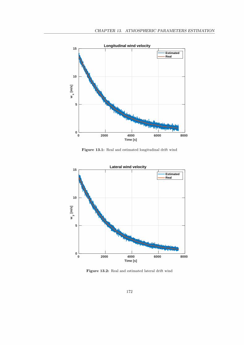
CHAPTER 13. ATMOSPHERIC PARAMETERS ESTIMATION
0 2000 4000 6000 8000Time [s]
0
5
10
15
wx [
m/s
]
Longitudinal wind velocity
EstimatedReal
Figure 13.1: Real and estimated longitudinal drift wind
0 2000 4000 6000 8000Time [s]
0
5
10
15
wy [
m/s
]
Lateral wind velocity
EstimatedReal
Figure 13.2: Real and estimated lateral drift wind
172

CHAPTER 13. ATMOSPHERIC PARAMETERS ESTIMATION
0 2000 4000 6000 8000Time [s]
-2
-1.5
-1
-0.5
0
0.5
1
1.5
2
wz [
m/s
]
Vertical wind velocity
EstimatedReal
Figure 13.3: Real and estimated vertical drift wind
0 2000 4000 6000 8000
Time [s]
0
0.2
0.4
0.6
0.8
1
1.2
1.4
1.6
1.8
err
or
[m/s
]
Monte Carlo simulation of wind field estimation
mix/max erroraverage errorpredicted error
Figure 13.4: Monte Carlo simulation results: drift wind
173

CHAPTER 13. ATMOSPHERIC PARAMETERS ESTIMATION
0 1000 2000 3000 4000 5000 6000 7000Time [s]
-3
-2
-1
0
1
2
3
wx [
m/s
]
Longitudinal wind velocity
EstimatedReal
Figure 13.5: Real and estimated longitudinal gust wind
0 1000 2000 3000 4000 5000 6000 7000Time [s]
-3
-2
-1
0
1
2
3
wy [
m/s
]
Lateral wind velocity
EstimatedReal
Figure 13.6: Real and estimated lateral gust wind
174

CHAPTER 13. ATMOSPHERIC PARAMETERS ESTIMATION
0 1000 2000 3000 4000 5000 6000 7000Time [s]
-3
-2
-1
0
1
2
3
wz [
m/s
]
Vertical wind velocity
EstimatedReal
Figure 13.7: Real and estimated vertical gust wind
0 2000 4000 6000 8000
Time [s]
0
0.2
0.4
0.6
0.8
1
1.2
1.4
1.6
1.8
err
or
[m/s
]
Monte Carlo simulation of wind field estimation
mix/max error
average error
predicted error
Figure 13.8: Monte Carlo simulation results: gust wind
175

CHAPTER 13. ATMOSPHERIC PARAMETERS ESTIMATION
0 2000 4000 6000 8000
Time [s]
0
0.2
0.4
0.6
0.8
1
1.2
1.4
1.6
1.8
2
err
or
[m/s
]
Monte Carlo simulation of wind field estimation
mix/max error
average error
predicted error
Figure 13.9: Monte Carlo simulation results: drift wind and maneuver
0 1000 2000 3000 4000 5000 6000
Time [s]
0
0.2
0.4
0.6
0.8
1
1.2
1.4
1.6
1.8
2
err
or
[m/s
]
Monte Carlo simulation of wind field estimation
mix/max erroraverage errorpredicted error
Figure 13.10: Monte Carlo simulation results: gust wind and maneuver
176

CHAPTER 13. ATMOSPHERIC PARAMETERS ESTIMATION
0 5 10 15 20 25 30error [%]
0
0.5
1
1.5
2
2.5
3
3.5
4h
[m
]
10 4 Wind forward prediction error
T=300 sT=650 sT=1110 sT=1650 sT=2300 sT=3000 s
Figure 13.11: Error of the wind forward prediction procedure performed at different time instantsduring the descent
0 5 10 15 20 25 30error [%]
0
0.5
1
1.5
2
2.5
3
3.5
4
h [
m]
10 4 On-going wind forward prediction error
On-going prediction
Figure 13.12: Overall error of the on-going wind forward prediction during the descent
177

CHAPTER 13. ATMOSPHERIC PARAMETERS ESTIMATION
0 1 2 3 4 5 6
[kg/m3
]
0
0.5
1
1.5
2
2.5
3
3.5
4
h [
m]
104 Density estimation
estimated
real
Figure 13.13: Real vs estimated density during the descent
0 1000 2000 3000 4000 5000 6000 7000t [s]
0
5
10
15
20
25
30
e [%
]
Density estimation percentage error
Figure 13.14: Density estimation percentage error
178

Chapter 14
Conclusions and future works
As affirmed in first pages of the thesis, the aim of the work was to demonstrate if the applicationof parafoils technology on planetary landing could bring advantages, exploiting parafoils highmaneuverability. At the final stage of the work and after all carried out analysis, it can be statedthat the idea of using parafoils to guide a landing vehicle through Titan atmosphere is reasonable:tools developed along the work can be useful to predict its trajectory and performances. Precisely:
• Low-fidelity models have been described and compared (from an analytical point of viewand through simulations). They can be useful to have a rough, easy and fast estimation ofmain performances with few input data (in terms of parafoil geometry and aerodynamiccharacterization). What has been learned from these analysis is that the analyzed descenttowards Titan lasts almost 2 hours, that the vertical touchdown velocity is between 3 m/sand 4 m/s and that the lateral wind causes a maximum drift in landing position of about40 km.
• A high-fidelity dynamical model has been analyzed in detail and used to simulate the de-scent. More precise values of all performances have been carried out and the relative angulardisplacement between payload and parafoil has been investigated. The most important as-pects learned are that the system flies at a pitch angle different from zero (precisely, thepitch angle assumes a negative value and this quantity is different for parafoil and payload)and that angle of attack modestly varies along the descent.
• A sensitivity analysis and some turn performances investigations have been realized. Look-ing to results presented in relative sections, what a parafoil is able to do to and what cannotbe done can be understood. Variation of geometrical or aerodynamics parafoil character-istics can lead to different performances: this fact will result very important in a possiblefuture stage of the work, when the parafoil will have to be effectively designed. Underliningthe most important output number, the maximum turn rate of the parafoil (which dependson altitude and maximum command deflection) goes from 22 deg/s at high altitude andbig maximum command deflection to about 2 deg/s at zero altitude and small maximumcommand deflection.
• An appropriate control logic for parafoil turn has been derived. The Nonlinear DynamicsInversion theory has been proposed as a good tool to calculate the necessary asymmet-ric deflection needed to follow a desired trajectory and a procedure meant to counteractlateral wind effects has been carried out. Through the simulation of different trajectoriesand wind conditions, the high maneuverability and versatility of the parafoil have been
179

CHAPTER 14. CONCLUSIONS AND FUTURE WORKS
demonstrated. An interesting numerical result which has been obtained is the fact thatthe diameter of the spiral maneuver performed to stay in proximity of the landing site isabout 600 m. Comparing this number with the landing site ”characteristic dimension”, thelanding feasibility can be studied. Another important obtained result is the demonstrationthat the system can well counteract the effect of a lateral blast of wind flying towards thedesired landing site with a non-zero asymmetric line deflection. Finally, the implementa-tion of the electric motor dynamics has shown that the actuation can be controlled throughthis type of hardware: consequences are that desired and effective deflection are slightlydifferent, due to the presence of the electrical dynamics.
• The gust wind issue has been deeply faced, understood and mitigated through the de-velopment of a payload attitude control scheme. The fact that reaction wheel cannot beused to adequately control payload attitude has been demonstrated. The control authoritynecessary for the fulfillment of camera pointing requirement (angles in the order of milli-radians) has been estimated in about 30 Nm. More than one actuator solutions have beenproposed: their feasibility will have to be deeply studied.
• With regard to atmospheric parameters, a wind estimation procedure has been developed.An error analysis has shown that maximum error does not exceed 2 m/s and that averageerror stays between 0.35 m/s and 0.55 m/s. The carried out Monte Carlo analysis hasshown the goodness of the procedure for both drift and gust wind and also during maneu-vers. After that, a possible way of predicting the lateral wind the parafoil will encounterduring the next phase of the descent on the basis of data measured on the first phase ofthe mission has been presented; the obtained error is in the order of 20 %, but it can besignificantly reduced performing the described least square minimization procedure morefrequently. Finally, a model-based density estimator made with an extended Kalman filterhas been developed: a simulation exhibits the goodness of the procedure showing an errorof the estimation which goes from 25% of the initial phases of the descent to less than 10%at the touchdown.
Wind is the most dangerous enemy of parafoils, and this fact has been well underlined alongthe entire work: thus, parafoils can be used for space applications as long as wind effects arecompletely handled, not to completely jeopardize the mission. The development of the wind esti-mation procedure and of the wind forward prediction method have the aim of showing how windcan become a known effect for the parafoil, giving it the possibility to autonomously counteractthe drift from the desired trajectory.
Possible developments of this research are mainly related to the introduction of better windmodels and to a deeper study of system deformation. Being systematic, possible future workscan be summarized in following aspects:
• In order to study how the actuation line deflection acts on the shape of the canopy (andso to understand how really an asymmetric actuation causes the turn of the parafoil) afinite element model of the canopy in which both structural and aerodynamics effects areconsidered shall be developed. Basically, the assumption of rigid body for the canopy andfor the suspension lines has to be removed. This consideration is supported by previousworks that can be found in literature. For example, according to [37], ”due to the flexibilityof the parachute structure, it is clear that fluid-structure interaction simulation is requiredto compute the parafoil inflated shape, based upon the equilibrium between structural andaerodynamics forces”; moreover, according to [38], ”in order to study wing deformationwithout relying in assumptions, a combined aerodynamic-structural analysis is necessary.
180

CHAPTER 14. CONCLUSIONS AND FUTURE WORKS
A well established method to compute structure deformations is the finite element methodwhich is applied here”.
• More accurate Titan drift wind models should be taken into account; the important char-acteristic they shall have is the dependence of wind velocity not only on the altitude butalso on the specific location above the planet (latitude and longitude) and on period ofthe year (season). This analysis could be useful to start understanding which is the bestperiod of the year to reach a precise landing site (useful to start sizing the system andthinking on the orbital transfer associated with the mission). A possible wind model tobe implemented is the Global-Circulation Model (hints on this topic are given in [25] andexperimental results are shown in [29]).
• In this work payload attitude control analysis has been carried out with a gust wind modelsuitable for the representation of terrestrial turbulence wind, since better data were notavailable. A Titan gust wind model should be used to simulate payload attitude control.Data can be made available as wind correlation time or length and wind velocity standarddeviation (adequately estimated) or as a set of wind measurements (which can possiblycome from Huygens data) on which gust wind parameters can be statistically computed.Without accurate data of this type the correct camera pointing cannot be assure and theeffective requested control authority cannot be calculated.
• Once that a better gust wind model has been used to simulate payload attitude control,the actuator set shall be selected once for all. In this work advantages and drawbacks ofeach solution have been analyzed; detailed simulations shall be run, integrating also cameraimages acquisition routine inside the model.
• In this work all simulations have been conducted using geometrical and aerodynamics pa-rameters and coefficients of a notional parafoil system: they have been retrieved fromliterature or appropriately scaled. Once that a real model of a Titan parachute will beavailable, real dimensions and aerodynamics coefficients shall be used to simulate the de-scent of this precise parafoil towards Titan surface, comparing simulated performances withparafoil features declared by the manufacturer.
• One last possible future work can be pointed out. A critical phase of a landing usingparafoil is the deployment of the parafoil itself, since it has to be released in such a waythat the canopy shape can give lift to the parafoil and stabilize its movement. Studies onthis aspect should be conducted in the future.
181


Bibliography
[1] Quadrelli, Marco B., and Acikmese, A. Behcet ”Planetary Aeromanuevering for precisionlanding” Advances in the Astronautical Sciences 120 (2005)
[2] Yakimenko, Oleg A. ”Precision Aerial Delivery Systems: Modeling, Dynamics, and Control”AIAA, Volume 248 Progress in Astronautics and Aeronautics, 2015
[3] Lingard, J. Stephen, and Ram-air Parachute Design. ”Precision Aerial Delivery Seminar.”13th AIAA Aerodynamic Decelerator Systems Technology Conference, Clearwater Beach.1995.
[4] Quadrelli, Marco B. ”A Novel Approach to Planetary Precision Landing using Parafoils.”Advances in the Astronautical Sciences 120 (2005): 229-244.
[5] Jann, Thomas. ”Aerodynamic Coefficients for a Parafoil Wing with Arc Anhedral: Theoreticaland Experimental Results.” AIAA Paper 2106 (2003): 19-22.
[6] Gockel, W. ”Computer Based Modeling and Analysis of a Parafoil-Load Vehicle, case study1.” Seminar at 14th AIAA ADS Conference, San Francisco. 1997.
[7] Lee, Seong-Jin, and Andrew S. Arena Jr. ”Autonomous Parafoil Return-to-Point Vehicle forHigh Altitude Ballooning.” AIAA Guidance, Navigation, and Control Conference. 2014.
[8] Lissaman, P., and GLEN BROWN. ”Apparent mass effects on parafoil dynamics.” AerospaceDesign Conference. 1993.
[9] Lingard, J. S. ”The Performance and Design of Ram-Air Parachutes.” Pr507 N. GranadaAve.ecision Aerial Delivery Seminar, Technical Report, Royal Aircraft Establishment, Aug.1981.
[10] Prakash, Om, and Narayan Ananthkrishnan. ”Modeling and simulation of 9-DOF parafoil-payload system flight dynamics.” AIAA Atmospheric Flight Mechanics Conference and Exhibit.2006.
[11] Ashley, Holt. ”Engineering analysis of flight vehicles.” Addison-Weslet Publishing Company,1974.
[12] Vinh, Nguyen. ”Optimal trajectories in atmospheric flight.” Vol. 2. Elsevier, 2012.
[13] Zipfel, Peter H. ”Modeling and simulation of aerospace vehicle dynamics.” Aiaa, 2000.
[14] Quadrelli, Marco B., Jonathan M. Cameron, and Viktor Kerzhanovich. ”Modeling, sim-ulation, and control of parachute/balloon flight systems for Mars exploration.” 16th AIAAAerodynamic Decelerator Systems Technology Conference and Seminar. 2001.
183

BIBLIOGRAPHY
[15] Slegers, Nathan, and Mark Costello. ”Aspects of control for a parafoil and payload system.”Journal of Guidance, Control, and Dynamics 26.6 (2003): 898-905.
[16] Toohey, Damian. ”Development of a small parafoil vehicle for precision delivery.” Diss.Massachusetts Institute of Technology, 2005.
[17] Iacomini, C., and C. Cerimele. ”Longitudinal aerodynamics from a large scale parafoil testprogram.” 15th Aerodynamic Decelerator Systems Technology Conference. 1999.
[18] Iacomini, C., and C. Cerimele. ”Lateral-directional aerodynamics from a large scale parafoiltest program.” 15th Aerodynamic Decelerator Systems Technology Conference. 1999.
[19] Machin, Ricardo, Jenny Stein, and John Muratore. ”An overview of the X-38 prototypecrew return vehicle development and test program.” 15th Aerodynamic Decelerator SystemsTechnology Conference. 1999.
[20] Lorenz, Ralph D. ”Attitude and angular rates of planetary probes during atmospheric de-scent: Implications for imaging.” Planetary and Space Science 58.5 (2010): 838-846.
[21] Quadrelli, Marco B., Jonathan M. Cameron, and Viktor Kerzhanovich. ”Multibody dynamicsof parachute and balloon flight systems for planetary exploration.” Journal of guidance, control,and dynamics 27.4 (2004): 564-571.
[22] Calise, Anthony, and Daniel Preston. ”Approximate correction of guidance commands forwinds.” 20th AIAA Aerodynamic Decelerator Systems Technology Conference and Seminar.2009.
[23] Carter, David, et al. ”Autonomous large parafoil guidance, navigation, and control systemdesign status.” 19th AIAA Aerodynamic Decelerator Systems Technology Conference andSeminar. 2007.
[24] Jann, Thomas. ”Advanced features for autonomous parafoil guidance, navigation and con-trol.” 18th AIAA Aerodynamic Decelerator Systems Technology Conference and Seminar.2005.
[25] Lorenz, Ralph D., et al. ”Formulation of a wind specification for Titan late polar summerexploration.” Planetary and Space Science 70.1 (2012): 73-83.
[26] Lorenz, Ralph D., and Claire E. Newman. ”Twilight on Ligeia: Implications of communica-tions geometry and seasonal winds for exploring Titan’s seas 2020-2040.” Advances in SpaceResearch 56.1 (2015): 190-204.
[27] Watkins, Simon, et al. ”Atmospheric winds and their implications for microair vehicles.”AIAA journal 44.11 (2006): 2591-2600.
[28] Langelaan, Jack W., Nicholas Alley, and James Neidhoefer. ”Wind field estimation for smallunmanned aerial vehicles.” Journal of Guidance, Control, and Dynamics 34.4 (2011): 1016-1030.
[29] Folkner, W. M., et al. ”Winds on Titan from ground based tracking of the Huygens probe.”Journal of Geophysical Research: Planets 111.E7 (2006).
[30] Crassidis, John L., and John L. Junkins. ”Optimal estimation of dynamic systems.” CRCpress, 2011.
184

BIBLIOGRAPHY
[31] Honeywell Aerospace Electronic Systems, ”Constellation series reaction wheels”, December2003, https://aerocontent.honeywell.com/aero/common/documents/Constellation_
Series_Reaction_Wheels.pdf
[32] Airbus Safran Launchers, ”Chemical Monopropellant Thruster Family”, http://www.
space-propulsion.com/brochures/hydrazine-thrusters/hydrazine-thrusters.pdf
[33] Airbus Defense and Space, ”CMG 15-45S Data-sheet”, https://spaceequipment.
airbusdefenceandspace.com/wp-content/uploads/2015/04/cmg-15-45s-datasheet.pdf
[34] Hughes, Peter C. ”Spacecraft attitude dynamics.” Courier Corporation, 2012.
[35] Braun, Robert D., and Robert M. Manning. ”Mars exploration entry, descent, and landingchallenges.” Journal of spacecraft and rockets 44.2 (2007): 310-323.
[36] Prakash, Ravi, et al. ”Mars Science Laboratory entry, descent, and landing systemoverview.” Aerospace Conference, 2008 IEEE. IEEE, 2008.
[37] Fogell, Nicholas A., et al. ”Fluid-structure interaction simulation of the inflated shape ofram-air parachutes.” AIAA Aerodynamic Decelerator Systems (ADS) Conference. 2013.
[38] Altmann, Horst. ”Numerical Simulation of Parafoil Aerodynamics and Dynamic Be-haviour.” 20th AIAA Aerodynamic Decelerator Systems Technology Conference and Seminar.2009.
[39] Karlgaard, Christopher D., and Mark Schoenenberger. ”Planetary Probe Entry AtmosphereEstimation Using Synthetic Air Data System.” Journal of Spacecraft and Rockets (2017): 1-12.
185