Embed Size (px)
Citation preview
Data Mining and Knowledge Discovery, 1, 343–373 (1997)c© 1997 Kluwer Academic Publishers. Manufactured in The Netherlands.
Parallel Algorithms for Discovery ofAssociation Rules
MOHAMMED J. ZAKI [email protected]
SRINIVASAN PARTHASARATHY [email protected]
MITSUNORI OGIHARA [email protected]
Department of Computer Science, University of Rochester, Rochester, NY 14627
WEI LI [email protected]
Oracle Corporation, 500 Oracle Parkway, M/S 4op9, Redwood Shores, CA 94065
Editors: Paul Stolorz and Ron Musick
Abstract. Discovery of association rules is an important data mining task. Several parallel and sequentialalgorithms have been proposed in the literature to solve this problem. Almost all of these algorithms makerepeated passes over the database to determine the set of frequentitemsets(a subset of database items), thusincurring high I/O overhead. In the parallel case, most algorithms perform a sum-reduction at the end of each passto construct the global counts, also incurring high synchronization cost.
In this paper we describe new parallel association mining algorithms. The algorithms use novel itemset clusteringtechniques to approximate the set of potentially maximal frequent itemsets. Once this set has been identified, thealgorithms make use of efficient traversal techniques to generate the frequent itemsets contained in each cluster.We propose two clustering schemes based on equivalence classes and maximal hypergraph cliques, and study twolattice traversal techniques based on bottom-up and hybrid search. We use a vertical database layout to clusterrelated transactions together. The database is also selectively replicated so that the portion of the database neededfor the computation of associations is local to each processor. After the initial set-up phase, the algorithms donot need any further communication or synchronization. The algorithms minimize I/O overheads by scanning thelocal database portion only twice. Once in the set-up phase, and once when processing the itemset clusters. Unlikeprevious parallel approaches, the algorithms use simple intersection operations to compute frequent itemsets anddo not have to maintain or search complex hash structures.
Our experimental testbed is a 32-processor DEC Alpha cluster inter-connected by the Memory Channel network.We present results on the performance of our algorithms on various databases, and compare it against a well knownparallel algorithm. The best new algorithm outperforms it by an order of magnitude.
Keywords: parallel data mining, association rules, maximal hypergraph cliques, lattice traversal
1. Introduction
With recent progress in automated data gathering, and the availability of cheap storage,a lot of businesses have routinely started collecting massive amounts of data on variousfacets of the organization. The eventual goal of this data gathering is to be able to usethis information to gain a competitive edge, by discovering previously unknown patternsin the data, which can guide the decision making. Such high-level inference process mayprovide a host of useful information on customer groups, buying patterns, stock trends,etc. This process of automatic information inferencing is commonly known as KnowledgeDiscovery and Data mining (KDD). We look at one of the central KDD tasks — mining for
5
344 ZAKI, PARTHASARATHY, OGIHARA AND LI
associations. Discovery of association rules is an important problem in database mining.The prototypical application is the analysis of sales orbasketdata (Agrawal, et al., 1996).Basket data consists of items bought by a customer along with the transaction identifier.Besides the retail sales example, association rules have been shown to be useful in domainssuch as decision support, telecommunications alarm diagnosis and prediction, universityenrollments, etc.
1.1. Problem Statement
The problem of mining associations over basket data was introduced in (Agrawal, Imielinski,& Swami, 1993). It can be formally stated as: LetI = {i1, i2, · · · , im}be a set ofmdistinctattributes, also calleditems. Each transactionT in the databaseD of transactions, has aunique identifier, andcontainsa set of items, calleditemset, such thatT ⊆ I, i.e. eachtransaction is of the form< TID, i1, i2, ..., ik >. An itemset withk items is called ak-itemset. A subset of lengthk is called ak-subset. An itemset is said to have asupports if s% of the transactions inD contain the itemset. Anassociation ruleis an expressionA ⇒ B, where itemsetsA,B ⊂ I, andA ∩ B = ∅. Theconfidenceof the associationrule, given assupport(A ∪ B)/support(A), is simply the conditional probability that atransaction containsB, given that it containsA. The data mining task for association rulescan be broken into two steps. The first step consists of finding allfrequentitemsets, i.e.,itemsets that occur in the database with a certain user-specified frequency, calledminimumsupport. The second step consists of forming conditional implication rules among thefrequent itemsets (Agrawal & Srikant, 1994). The second step is relatively straightforward.Once the support of frequent itemsets is known, rules of the formX − Y ⇒ Y (whereY ⊂ X), are generated for all frequent itemsetsX, provided the rules meet a desiredconfidence. On the other hand the problem of identifying all frequent itemsets is hard.Givenm items, there are potentially2m frequent itemsets, which form alattice of subsetsoverI. However, only a small fraction of the whole lattice space is frequent. Discoveringthe frequent itemsets requires a lot of computation power, memory and disk I/O, which canonly be provided by parallel computers. Efficient parallel methods are needed to discoverthe relevant itemsets, and this is the focus of our paper.
1.2. Related Work
Sequential Algorithms Several algorithms for mining associations have been proposedin the literature. TheApriori algorithm (Mannila, Toivonen, & Verkamo, 1994; Agrawal& Srikant, 1994; Agrawal, et al., 1996) was shown to have superior performance to earlierapproaches (Agrawal, Imielinski, & Swami, 1993; Park, Chen, & Yu, 1995a; Holsheimer,et al., 1995; Houtsma & Swami, 1995) and forms the core of almost all of the currentalgorithms. Apriori uses thedownward closureproperty of itemset support to prune theitemset lattice – the property that all subsets of a frequent itemset must themselves befrequent. Thus only the frequentk-itemsets are used to constructcandidate(k + 1)-itemsets. A pass over the database is made at each level to find the frequent itemsets among
6
PARALLEL ASSOCIATION RULES 345
the candidates. For very large disk resident databases, these algorithms incur high I/Ooverhead for scanning it in each iteration. ThePartition algorithm (Savasere, Omiecinski,& Navathe, 1995) minimizes I/O by scanning the database only twice. It partitions thedatabase into small chunks which can be handled in memory. In the first pass it generatesthe set of all potentially frequent itemsets (any itemset locally frequent in a partition), andin the second pass their global support is obtained. Another way to minimize the I/Ooverhead is to work with only a small random sample of the database (Toivonen, 1996;Zaki, et al., 1997a). We recently proposed new algorithms (Zaki, et al., 1997b) which scanthe database only once, generating all frequent itemsets. These new algorithms were shownto outperform previousApriori based approaches by more than an order of magnitude (Zaki,et al., 1997b). The performance gains are obtained by using effective itemset clusteringand lattice traversal techniques. This paper presents efficient parallel implementations ofthese new algorithms.
Parallel Algorithms There has been relatively less work in parallel mining of associa-tions. Three different parallelizations ofApriori on a distributed-memory machine (IBMSP2) were presented in (Agrawal & Shafer, 1996). TheCount Distributionalgorithm isa straight-forward parallelization ofApriori. Each processor generates the partial sup-port of all candidate itemsets from its local database partition. At the end of each it-eration the global supports are generated by exchanging the partial supports among allthe processors. TheData Distribution algorithm partitions the candidates into disjointsets, which are assigned to different processors. However to generate the global sup-port each processor must scan the entire database (its local partition, and all the remotepartitions) in all iterations. It thus suffers from huge communication overhead. TheCan-didate Distributionalgorithm also partitions the candidates, but it selectively replicatesthe database, so that each processor proceeds independently. The local database por-tion is still scanned in every iteration.Count Distributionwas shown to have superiorperformance among these three algorithms (Agrawal & Shafer, 1996). Other parallel al-gorithms improving upon these ideas in terms of communication efficiency, or aggregatememory utilization have also been proposed (Cheung, et al., 1996b; Cheung, et al., 1996a;Han, Karypis, & Kumar, 1997). The PDM algorithm (Park, Chen, & Yu, 1995b) presents aparallelization of the DHP algorithm (Park, Chen, & Yu, 1995a). However, PDM performsworse thanCount Distribution(Agrawal & Shafer, 1996). In recent work we presented theCCPD parallel algorithm for shared-memory machines (Zaki, et al., 1996). It is similarin spirit to Count Distribution. The candidate itemsets are generated in parallel and arestored in a hash structure which is shared among all the processors. Each processor thenscans its logical partition of the database and atomically updates the counts of candidatesin the shared hash tree. CCPD uses additional optimization such as candidate balancing,hash-tree balancing and short-circuited subset counting to speed up performance (Zaki, etal., 1996). We also presented a new parallel algorithmEclat (Zaki, Parthasarathy, & Li,1997) on a DEC Alpha Cluster.Eclatuses the equivalence class itemset clustering schemealong with a bottom-up lattice traversal. It was shown to outperformCount Distributionby more than an order of magnitude. This paper will present parallelization results on newclustering and traversal techniques.
7
346 ZAKI, PARTHASARATHY, OGIHARA AND LI
1.3. Contribution
The main limitation of all the current parallel algorithms (Park, Chen, & Yu, 1995b; Zaki,et al., 1996; Agrawal & Shafer, 1996; Cheung, et al., 1996b; Cheung, et al., 1996a) isthat they make repeated passes over the disk-resident database partition, incurring high I/Ooverhead. Furthermore, the schemes involve exchanging either the counts of candidates orthe remote database partitions during each iteration. This results in high communication andsynchronization overhead. The previous algorithms also use complicated hash structureswhich entails additional overhead in maintaining and searching them, and typically sufferfrom poor cache locality (Parthasarathy, Zaki, & Li, 1997).
Our work contrasts to these approaches in several ways. We present new parallel algo-rithms for fast discovery of association rules based on our ideas in (Zaki, Parthasarathy,& Li, 1997; Zaki, et al., 1997b). The new parallel algorithms are characterized in termsof the clustering information used to group related itemsets, and in terms of the latticetraversal schemes used to search for frequent itemsets. We propose two clustering schemesbased on equivalence classes and maximal uniform hypergraph cliques, and we utilizetwo lattice traversal schemes, based on bottom-up and hybrid top-down/bottom-up search.The algorithms also use a different database layout which clusters related transactions to-gether, and the work is distributed among the processors in such a way that each processorcan compute the frequent itemsets independently, using simple intersection operations.An interesting benefit of using simple intersections is that the algorithms we propose canbe implemented directly on general purpose database systems (Holsheimer, et al., 1995;Houtsma & Swami, 1995). These techniques eliminate the need for synchronization afterthe initial set-up phase, and enable us to scan the database only two times, drastically cut-ting down the I/O overhead. Our experimental testbed is a 32-processor DEC Alpha SMPcluster (8 hosts, 4 processors/host) inter-connected by the Memory Channel (Gillett, 1996)network. The new parallel algorithms are also novel in that they utilize this machine config-uration information, i.e., they assume a distributed-memory model across the 8 cluster hosts,but assume a shared-memory model for the 4 processors on each host. We experimentallyshow that our new algorithms outperform the well knownCount Distributionalgorithm.We also present extensive performance results on their speedup, sizeup, communicationcost and memory usage.
The rest of the paper is organized as follows. We begin by providing more details onthe sequentialApriori algorithm. Section 3 describes some of the previousApriori basedparallel algorithms. We then present the main ideas behind our new algorithms – the itemsetand transaction clustering, and the lattice traversal techniques, in section 4. Section 5describes the design and implementation of the new parallel algorithms. Our experimentalstudy is presented in section 6, and our conclusions in section 7.
2. SequentialApriori Algorithm
In this section we will briefly describe theApriori algorithm (Agrawal, et al., 1996), sinceit forms the core of all parallel algorithms (Agrawal & Shafer, 1996; Cheung, et al., 1996b;Cheung, et al., 1996a; Han, Karypis, & Kumar, 1997; Park, Chen, & Yu, 1995b; Zaki, et
8
PARALLEL ASSOCIATION RULES 347
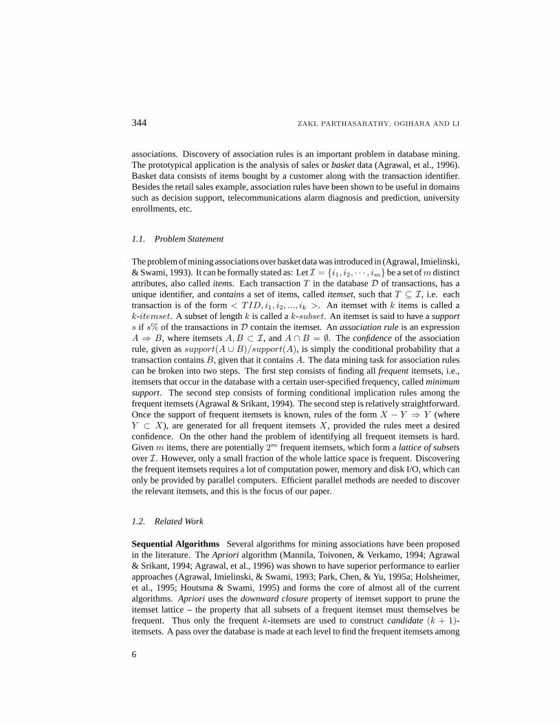
al., 1996).Apriori uses the downward closure property of itemset support that any subsetof a frequent itemset must also be frequent. Thus during each iteration of the algorithmonly the itemsets found to be frequent in the previous iteration are used to generate anew candidate set. A pruning step eliminates any candidate at least one of whose subsetsis not frequent. The complete algorithm is shown in table 1. It has three main steps.The candidates for thek-th pass are generated by joiningLk−1 with itself, which can beexpressed as:Ck = {X = A[1]A[2]...A[k − 1]B[k − 1]}, for all A,B ∈ Lk−1, withA[1 : k − 2] = B[1 : k − 2], andA[k − 1] < B[k − 1], whereX[i] denotes thei-th item,andX[i : j] denotes items at indexi throughj in itemsetX. For example, letL2 = {AB,AC, AD, AE, BC, BD, BE, DE}. ThenC3 = {ABC, ABD, ABE, ACD, ACE, ADE, BCD,BCE, BDE}.
Table 1.TheApriori Algorithm
1. L1 = {frequent 1-itemsets};2. for (k = 2;Lk−1 6= ∅; k + +)
3. Ck = Set of New Candidates;
4. for all transactionst ∈ D5. for all k-subsetss of t
6. if (s ∈ Ck) s.count+ +;
7. Lk = {c ∈ Ck|c.count ≥ minimum support};8. Set of all frequent itemsets =
⋃kLk;
Before inserting an itemset intoCk, Apriori tests whether all its(k − 1)-subsets arefrequent. Thispruningstep can eliminate a lot of unnecessary candidates. The candidates,Ck, are stored in a hash tree to facilitate fast support counting. An internal node of thehash tree at depthd contains a hash table whose cells point to nodes at depthd+ 1. All theitemsets are stored in the leaves. The insertion procedure starts at the root, and hashing onsuccessive items, inserts a candidate in a leaf. For countingCk, for each transaction in thedatabase, allk-subsets of the transaction are generated in lexicographical order. Each subsetis searched in the hash tree, and the count of the candidate incremented if it matches thesubset. This is the most compute intensive step of the algorithm. The last step formsLk byselecting itemsets meeting the minimum support criterion. For details on the performancecharacteristics ofApriori we refer the reader to (Agrawal & Srikant, 1994).
3. Apriori-based Parallel Algorithms
In this section we will look at some previous parallel algorithms. These algorithms assumethat the database is partitioned among all the processors in equal-sized blocks, which resideon the local disk of each processor.
TheCount Distributionalgorithm (Agrawal & Shafer, 1996) is a simple parallelizationof Apriori. All processors generate the entire candidate hash tree fromLk−1. Each pro-
9
348 ZAKI, PARTHASARATHY, OGIHARA AND LI
cessor can thus independently get partial supports of the candidates from its local databasepartition. This is followed by a sum-reduction to obtain the global counts. Note that onlythe partial counts need to be communicated, rather than merging different hash trees, sinceeach processor has a copy of the entire tree. Once the globalLk has been determinedeach processor buildsCk+1 in parallel, and repeats the process until all frequent item-sets are found. This simple algorithm minimizes communication since only the countsare exchanged among the processors. However, since the entire hash tree is replicated oneach processor, it doesn’t utilize the aggregate memory efficiently. The implementation ofCount Distributionused for comparison in our experiments differs slightly from the abovedescription and is optimized for our testbed configuration. Only one copy of the hash treeresides on each of the 8 hosts in our cluster. All the 4 processors on each host share thishash tree. Each processor still has its own local database portion and uses a local array togather the local candidate support. The sum-reduction is accomplished in two steps. Thefirst step performs the reduction only among the local processors on each host. The secondstep performs the reduction among the hosts. We also utilize some optimization techniquessuch as hash-tree balancing and short-circuited subset counting (Zaki, et al., 1996) to furtherimprove the performance ofCount Distribution.
TheData Distributionalgorithm (Agrawal & Shafer, 1996) was designed to utilize thetotal system memory by generating disjoint candidate sets on each processor. However togenerate the global support each processor must scan the entire database (its local partition,and all the remote partitions) in all iterations. It thus suffers from high communicationoverhead, and performs very poorly when compared toCount Distribution(Agrawal &Shafer, 1996).
TheCandidate Distributionalgorithm (Agrawal & Shafer, 1996) uses a property of fre-quent itemsets (Agrawal & Shafer, 1996; Zaki, et al., 1996) to partition the candidatesduring iterationl, so that each processor can generate disjoint candidates independent ofother processors. At the same time the database is selectively replicated so that a processorcan generate global counts independently. The choice of the redistribution pass involves atrade-off between decoupling processor dependence as soon as possible and waiting untilsufficient load balance can be achieved. In their experiments the repartitioning was done inthe fourth pass. After this the only dependence a processor has on other processors is forpruning the candidates. Each processor asynchronously broadcasts the local frequent setto other processors during each iteration. This pruning information is used if it arrives intime, otherwise it is used in the next iteration. Note that each processor must still scan itslocal data once per iteration. Even though it uses problem-specific information, it performsworse thanCount Distribution(Agrawal & Shafer, 1996).Candidate Distributionpays thecost of redistributing the database, and it then scans the local database partition repeatedly,which will usually be larger than||D||/P .
4. Efficient Clustering and Traversal Techniques
In this section we present our techniques to cluster related frequent itemsets together usingequivalence classes and maximal uniform hypergraph cliques. We then describe the bottom-up and hybrid itemset lattice traversal techniques. We also present a technique to cluster
10
PARALLEL ASSOCIATION RULES 349
related transactions together by using the vertical database layout. This layout is able tobetter exploit the proposed clustering and traversal schemes. It also facilitates fast itemsetsupport counting using simple intersections, rather than maintaining and searching complexdata structures.
4.1. Itemset Clustering
123 124 125 134 135 145 234 235 245 345
12345
1234 1235 1245 1345 2345
1 2 3 4 5
12 13 14 15 23 24 3525 34 45
Lattice of Subsets of {1,2,3,4,5}
Border ofFrequent Itemsets
1 2 3 4 3 4 5
35 4534
345
12 13 14 23 24 34
234123 134124
1234
Lattice of Subsets of {1,2,3,4}
Lattice of Subsets of {3,4,5}
Sublattices Induced by Maximal Itemsets
Figure 1. Lattice of Subsets and Maximal Itemset Induced Sub-lattices
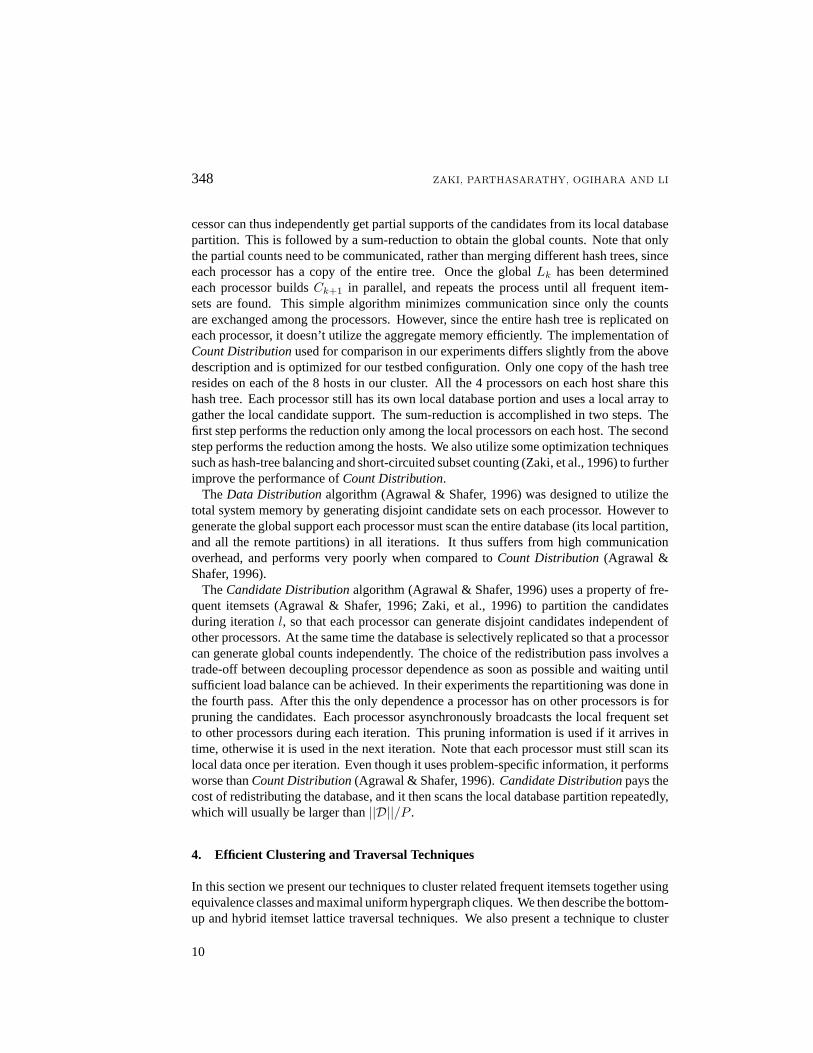
We will motivate the need for itemset clustering by means of an example. Consider thelattice of subsets of the set{1, 2, 3, 4, 5}, shown in figure 1 (the empty set has been omittedin all figures). The frequent itemsets are shown with dashed circles and the twomaximalfrequent itemsets (a frequent itemset ismaximalif it is not a proper subset of any otherfrequent itemset) are shown with the bold circles. Due to the downward closure propertyof itemset support – the fact that all subsets of a frequent itemset must be frequent – thefrequent itemsets form aborder, such that all frequent itemsets lie below the border, whileall infrequent itemsets lie above it. The border of frequent itemsets is shown with a boldline in figure 1. An optimal association mining algorithm will only enumerate and testthe frequent itemsets, i.e., the algorithm must efficiently determine the structure of theborder. This structure is precisely determined by the maximal frequent itemsets. Theborder corresponds to the sub-lattices induced by the maximal frequent itemsets. Thesesub-lattices are shown in figure 1.
11
350 ZAKI, PARTHASARATHY, OGIHARA AND LI
Given the knowledge of the maximal frequent itemsets we can design an efficient algo-rithm that simply gathers their support and the support of all their subsets in just a singledatabase pass. In general we cannot precisely determine the maximal itemsets in the in-termediate steps of the algorithm. However we can approximate this set. Our itemsetclustering techniques are designed to group items together so that we obtain supersets ofthe maximal frequent itemsets – thepotential maximal frequent itemsets. Below we presenttwo schemes to generate the set of potential maximal itemsets based on equivalence classesand maximal uniform hypergraph cliques. These two techniques represent a trade-off inthe precision of the potential maximal itemsets generated, and the computation cost. Thehypergraph clique approach gives more precise information at higher computation cost,while the equivalence class approach sacrifices quality for a lower computation cost.
4.1.1. Equivalence Class Clustering
Let’s reconsider the candidate generation step ofApriori. Let L2 = {AB, AC, AD, AE,BC, BD, BE, DE}. ThenC3 = { ABC, ABD, ABE, ACD, ACE, ADE, BCD, BCE, BDE}.Assuming thatLk−1 is lexicographically sorted, we can partition the itemsets inLk−1 intoequivalence classesbased on their commonk−2 length prefixes, i.e., the equivalence classa ∈ Lk−2, is given as:
Sa = [a] = {b[k − 1] ∈ L1 | a[1 : k − 2] = b[1 : k − 2]}
Candidatek-itemsets can simply be generated from itemsets within a class by joining all(|Si|2
)pairs, with the the class identifier as the prefix. For our exampleL2 above, we obtain
the equivalence classes:SA = [A] = {B, C, D, E}, SB = [B] = {C, D, E}, andSD = [D]= {E}. We observe that itemsets produced by the equivalence class[A] , namely those inthe set{ABC, ABD, ABE, ACD, ACE, ADE}, are independent of those produced by theclass[B] (the set{BCD, BCE, BDE}). Any class with only 1 member can be eliminatedsince no candidates can be generated from it. Thus we can discard the class[D] . This ideaof partitioningLk−1 into equivalence classes was independently proposed in (Agrawal &Shafer, 1996; Zaki, et al., 1996). The equivalence partitioning was used in (Zaki, et al.,1996) to parallelize the candidate generation step in CCPD. It was also used inCandidateDistribution (Agrawal & Shafer, 1996) to partition the candidates into disjoint sets.
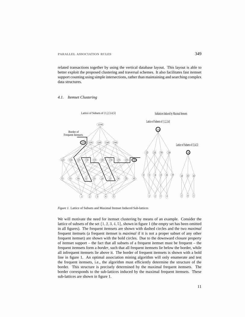
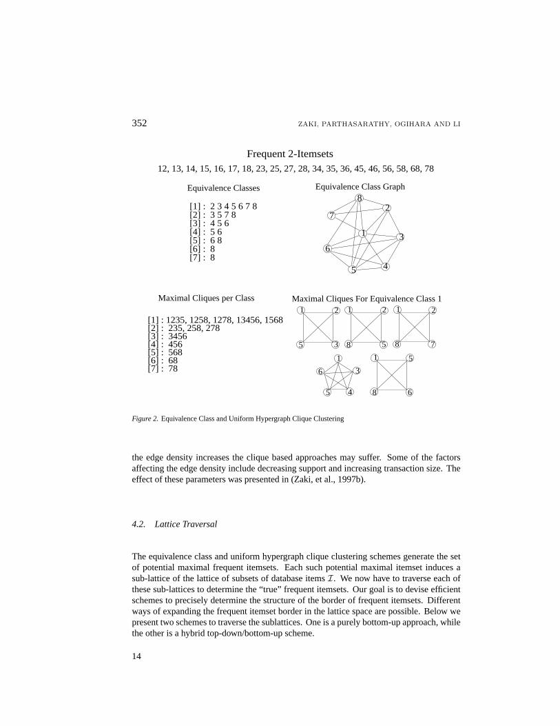
At any intermediate step of the algorithm when the set of frequent itemsets,Lk fork ≥ 2, has been determined we can generate the set of potential maximal frequent itemsetsfrom Lk. Note that fork = 1 we end up with the entire item universe as the maximalitemset. However, For anyk ≥ 2, we can extract more precise knowledge about theassociation among the items. The larger the value ofk the more precise the clustering. Forexample, figure 2 shows the equivalence classes obtained for the instance wherek = 2.Each equivalence class is a potential maximal frequent itemset. For example, the class[1],generates the maximal itemset 12345678.
12
PARALLEL ASSOCIATION RULES 351
4.1.2. Maximal Uniform Hypergraph Clique Clustering
Let the set of itemsI denote the vertex set. Ahypergraph(Berge, 1989) onI is a familyH = {E1, E2, ..., En} of edges or subsets ofI, such thatEi 6= ∅, and∪ni=1Ei = I. Asimple hypergraphis a hypergraph such that,Ei ⊂ Ej ⇒ i = j. A simple graph is asimple hypergraph each of whose edges has cardinality 2. The maximum edge cardinalityis called therank, r(H) = maxj |Ej |. If all edges have the same cardinality, thenHis called auniform hypergraph. A simple uniform hypergraph of rankr is called ar-uniformhypergraph. For a subsetX ⊂ I, thesub-hypergraphinduced byX is given as,HX = {Ej ∩ X 6= ∅|1 ≤ j ≤ n}. A r-uniform complete hypergraphwith m vertices,denoted asKr
m, consists of all ther-subsets ofI. A r-uniform complete sub-hypergraph iscalled ar-uniform hypergraph clique. A hypergraph clique ismaximalif it is not containedin any other clique. For hypergraphs of rank 2, this corresponds to the familiar concept ofmaximal cliques in a graph.
Given the set of frequent itemsetsLk, it is possible to further refine the clustering processproducing a smaller set of potentially maximal frequent itemsets. The key observationused is that given any frequentm-itemset, form > k, all its k-subsets must be frequent.In graph-theoretic terms, if each item is a vertex in the hypergraph, and eachk-subset anedge, then the frequentm-itemset must form ak-uniform hypergraph clique. Furthermore,the set of maximal hypergraph cliques represents an approximation or upper-bound on theset of maximal potential frequent itemsets. All the “true” maximal frequent itemsets arecontained in the vertex set of the maximal cliques, as stated formally in the lemma below.
Lemma 1 LetHLk be the k-uniform hypergraph with vertex setI, and edge setLk. LetC be the set of maximal hypergraph cliques inH, i.e.,C = {Kk
m|m > k}, and letM bethe set of vertex sets of the cliques inC. Then for all maximal frequent itemsetsf , ∃t ∈M ,such thatf ⊆ t.
An example of uniform hypergraph clique clustering is given in figure 2. The example isfor the case ofL2, and thus corresponds to an instance of the general clustering technique,which reduces to the case of finding maximal cliques in regular graphs. The figure shows allthe equivalence classes, and the maximal cliques within them. It also shows the graph forclass 1, and the maximal cliques in it. It can be seen immediately the the clique clusteringis more accurate than equivalence class clustering. For example, while equivalence classclustering produced the potential maximal frequent itemset 12345678, the hypergraph cliqueclustering produces a more refined set{1235, 1258, 1278, 13456, 1568} for equivalenceclass[1]. The maximal cliques are discovered using a dynamic programming algorithm.For a class[x] , andy ∈[x] ,y is said tocoverthe subset of[x] , given bycov(y) = [y]∩[x]. Foreach classC, we first identify itscovering set, given as{y ∈ C|cov(y) 6= ∅, andcov(y) 6⊆cov(z), for anyz ∈ C, z < y}. We recursively generate the maximal cliques for elementsin the covering set for each class. Each maximal clique from the covering set is prefixedwith the class identifier (eliminating any duplicates) to obtain the maximal cliques for thecurrent class (see (Zaki, et al., 1997c) for details). For general graphs the maximal cliquedecision problem is NP-Complete (Garey & Johnson, 1979). However, the equivalenceclass graph is usually sparse and the maximal cliques can be enumerated efficiently. As
13
352 ZAKI, PARTHASARATHY, OGIHARA AND LI
1 1 1
1
2 2 2
35 5
5
6
78 8
8
3
1
45
6
12, 13, 14, 15, 16, 17, 18, 23, 25, 27, 28, 34, 35, 36, 45, 46, 56, 58, 68, 78
Frequent 2-Itemsets
1 3
45
7
8
6
2
Equivalence Class Graph
Maximal Cliques For Equivalence Class 1Maximal Cliques per Class
[1] : 2 3 4 5 6 7 8[2] : 3 5 7 8[3] : 4 5 6 [4] : 5 6[5] : 6 8[6] : 8[7] : 8
Equivalence Classes
[1] : 1235, 1258, 1278, 13456, 1568[2] : 235, 258, 278[3] : 3456 [4] : 456[5] : 568[6] : 68[7] : 78
Figure 2. Equivalence Class and Uniform Hypergraph Clique Clustering
the edge density increases the clique based approaches may suffer. Some of the factorsaffecting the edge density include decreasing support and increasing transaction size. Theeffect of these parameters was presented in (Zaki, et al., 1997b).
4.2. Lattice Traversal
The equivalence class and uniform hypergraph clique clustering schemes generate the setof potential maximal frequent itemsets. Each such potential maximal itemset induces asub-lattice of the lattice of subsets of database itemsI. We now have to traverse each ofthese sub-lattices to determine the “true” frequent itemsets. Our goal is to devise efficientschemes to precisely determine the structure of the border of frequent itemsets. Differentways of expanding the frequent itemset border in the lattice space are possible. Below wepresent two schemes to traverse the sublattices. One is a purely bottom-up approach, whilethe other is a hybrid top-down/bottom-up scheme.
14
PARALLEL ASSOCIATION RULES 353
1516 13 14 1212 13 14 15 16150 200 400 500300
ItemsetSupport
Cluster: Potential Maximal Frequent Itemset (123456)
Sort Itemsets by Support
Top-Down Phase
Bottom-Up Phase
156
1356
13456
123456
16 15 13 14 12
1235
126 125 123 124
1516 13 14 12
BOTTOM-UP TRAVERSAL
True Maximal Frequent Itemsets: 1235, 13456
123 124 125 126 134 135 136 145 156146
12 13 14 15 16
1235 1456135613461345
13456
HYBRID TRAVERSAL
Figure 3. Bottom-up and Hybrid Lattice Traversal
4.2.1. Bottom-up Lattice Traversal
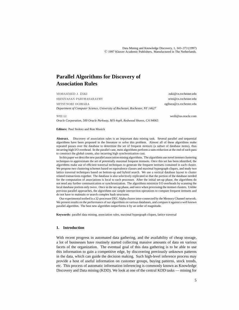
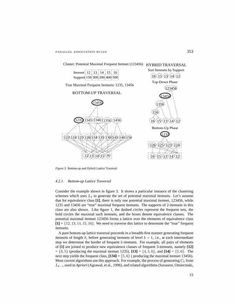
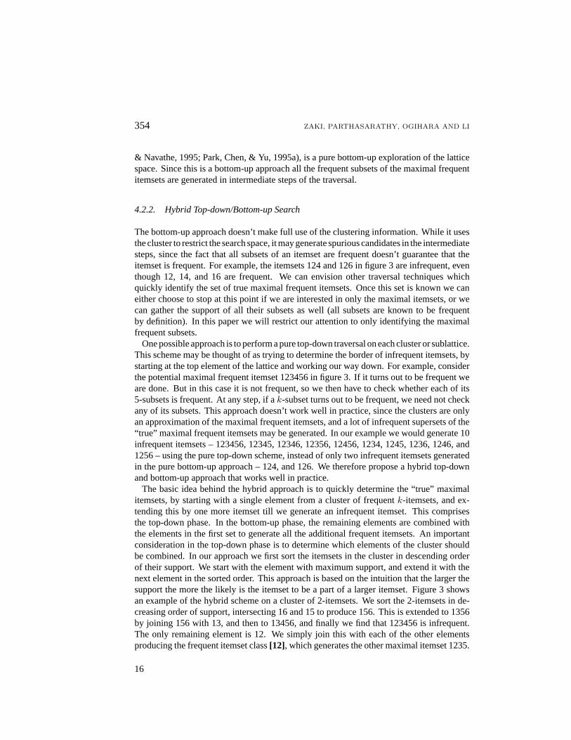
Consider the example shown in figure 3. It shows a particular instance of the clusteringschemes which usesL2 to generate the set of potential maximal itemsets. Let’s assumethat for equivalence class[1], there is only one potential maximal itemset, 123456, while1235 and 13456 are “true” maximal frequent itemsets. The supports of 2-itemsets in thisclass are also shown. Like figure 1, the dashed circles represent the frequent sets, thebold circles the maximal such itemsets, and the boxes denote equivalence classes. Thepotential maximal itemset 123456 forms a lattice over the elements of equivalence class[1] = {12, 13, 14, 15, 16}. We need to traverse this lattice to determine the “true” frequentitemsets.
A pure bottom-up lattice traversal proceeds in a breadth-first manner generating frequentitemsets of lengthk, before generating itemsets of levelk + 1, i.e., at each intermediatestep we determine the border of frequentk-itemsets. For example, all pairs of elementsof [1] are joined to produce new equivalence classes of frequent 3-itemsets, namely[12]= {3, 5} (producing the maximal itemset 1235),[13] = {4, 5, 6}, and[14] = {5, 6}. Thenext step yields the frequent class,[134] = {5, 6} ( producing the maximal itemset 13456).Most current algorithms use this approach. For example, the process of generatingCk fromLk−1 used inApriori (Agrawal, et al., 1996), and related algorithms (Savasere, Omiecinski,
15
354 ZAKI, PARTHASARATHY, OGIHARA AND LI
& Navathe, 1995; Park, Chen, & Yu, 1995a), is a pure bottom-up exploration of the latticespace. Since this is a bottom-up approach all the frequent subsets of the maximal frequentitemsets are generated in intermediate steps of the traversal.
4.2.2. Hybrid Top-down/Bottom-up Search
The bottom-up approach doesn’t make full use of the clustering information. While it usesthe cluster to restrict the search space, it may generate spurious candidates in the intermediatesteps, since the fact that all subsets of an itemset are frequent doesn’t guarantee that theitemset is frequent. For example, the itemsets 124 and 126 in figure 3 are infrequent, eventhough 12, 14, and 16 are frequent. We can envision other traversal techniques whichquickly identify the set of true maximal frequent itemsets. Once this set is known we caneither choose to stop at this point if we are interested in only the maximal itemsets, or wecan gather the support of all their subsets as well (all subsets are known to be frequentby definition). In this paper we will restrict our attention to only identifying the maximalfrequent subsets.
One possible approach is to perform a pure top-down traversal on each cluster or sublattice.This scheme may be thought of as trying to determine the border of infrequent itemsets, bystarting at the top element of the lattice and working our way down. For example, considerthe potential maximal frequent itemset 123456 in figure 3. If it turns out to be frequent weare done. But in this case it is not frequent, so we then have to check whether each of its5-subsets is frequent. At any step, if ak-subset turns out to be frequent, we need not checkany of its subsets. This approach doesn’t work well in practice, since the clusters are onlyan approximation of the maximal frequent itemsets, and a lot of infrequent supersets of the“true” maximal frequent itemsets may be generated. In our example we would generate 10infrequent itemsets – 123456, 12345, 12346, 12356, 12456, 1234, 1245, 1236, 1246, and1256 – using the pure top-down scheme, instead of only two infrequent itemsets generatedin the pure bottom-up approach – 124, and 126. We therefore propose a hybrid top-downand bottom-up approach that works well in practice.
The basic idea behind the hybrid approach is to quickly determine the “true” maximalitemsets, by starting with a single element from a cluster of frequentk-itemsets, and ex-tending this by one more itemset till we generate an infrequent itemset. This comprisesthe top-down phase. In the bottom-up phase, the remaining elements are combined withthe elements in the first set to generate all the additional frequent itemsets. An importantconsideration in the top-down phase is to determine which elements of the cluster shouldbe combined. In our approach we first sort the itemsets in the cluster in descending orderof their support. We start with the element with maximum support, and extend it with thenext element in the sorted order. This approach is based on the intuition that the larger thesupport the more the likely is the itemset to be a part of a larger itemset. Figure 3 showsan example of the hybrid scheme on a cluster of 2-itemsets. We sort the 2-itemsets in de-creasing order of support, intersecting 16 and 15 to produce 156. This is extended to 1356by joining 156 with 13, and then to 13456, and finally we find that 123456 is infrequent.The only remaining element is 12. We simply join this with each of the other elementsproducing the frequent itemset class[12], which generates the other maximal itemset 1235.
16
PARALLEL ASSOCIATION RULES 355
The bottom-up and hybrid approaches are contrasted in figure 3, and the pseudo-code forboth schemes is shown in table 3.
4.3. Transaction Clustering: Database Layout
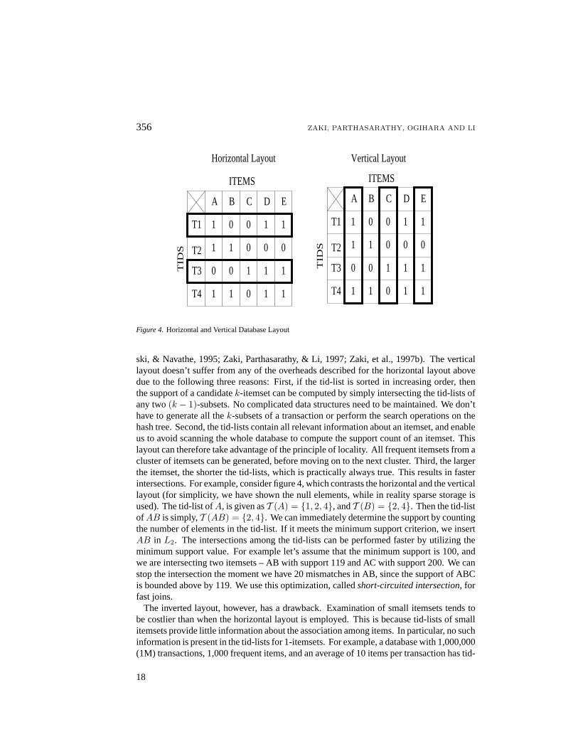
The KDD process consists of various steps (Fayyad, Piatetsky-Shapiro, & Smyth, 1996).The initial step consists of creating the target dataset by focusing on certain attributes or viadata samples. The database creation may require removing unnecessary information andsupplying missing data, and transformation techniques for data reduction and projection.The user must then determine the data mining task and choose a suitable algorithm, forexample, the discovery of association rules. The next step involves interpreting the dis-covered associations, possibly looping back to any of the previous steps, to discover moreunderstandable patterns. An important consideration in the data preprocessing step is thefinal representation or data layout of the dataset. Another issue is whether some preliminaryinvariant information can be gleaned during this process. There are two possible layouts ofthe target dataset for association mining – the horizontal and the vertical layout.
4.3.1. Horizontal Data Layout
This is the format standardly used in the literature (see e.g., (Agrawal & Srikant, 1994;Mannila, Toivonen, & Verkamo, 1994; Agrawal, et al., 1996)). Here a dataset consists ofa list of transactions. Each transaction has a transaction identifier (TID) followed by a listof items in that transaction. This format imposes some computation overhead during thesupport counting step. In particular, for each transaction of average lengthl, during iterationk, we have to generate and test whether all
(lk
)k-subsets of the transaction are contained
in Ck. To perform fast subset checking the candidates are stored in a complex hash-treedata structure. Searching for the relevant candidates thus adds additional computationoverhead. Furthermore, the horizontal layout forces us to scan the entire database or thelocal partition once in each iteration. BothCountandCandidate Distributionmust pay theextra overhead entailed by using the horizontal layout. Furthermore, the horizontal layoutseems suitable only for the bottom-up exploration of the frequent border. It appears to beextremely complicated to implement the hybrid approach using the horizontal format. Analternative approach is to store all the potential maximal itemsets and all their subsets ina data structure with fast look-up, (e.g., hash-trees (Agrawal, et al., 1996)). We can thengather their support in a single database scan. We plan to explore this in a later paper.
4.3.2. Vertical Data Layout
In the vertical (or inverted) layout (also called thedecomposed storage structure(Hol-sheimer, et al., 1995)), a dataset consists of a list of items, with each item followed byits tid-list — the list of all the transactions identifiers containing the item. An example ofsuccessful use of this layout can be found in (Holsheimer, et al., 1995; Savasere, Omiecin-
17
356 ZAKI, PARTHASARATHY, OGIHARA AND LI
A B C D E
1 0 0 1 1
1 1 0 0 0
1 1 100
1111 0
T2
T4
T1
T3
ITEMS
TID
S
A B C D E
1 0 0 1 1
1 1 0 0 0
1 1 100
1111 0
T2
T4
T1
T3
ITEMST
IDS
Horizontal Layout Vertical Layout
Figure 4. Horizontal and Vertical Database Layout
ski, & Navathe, 1995; Zaki, Parthasarathy, & Li, 1997; Zaki, et al., 1997b). The verticallayout doesn’t suffer from any of the overheads described for the horizontal layout abovedue to the following three reasons: First, if the tid-list is sorted in increasing order, thenthe support of a candidatek-itemset can be computed by simply intersecting the tid-lists ofany two(k − 1)-subsets. No complicated data structures need to be maintained. We don’thave to generate all thek-subsets of a transaction or perform the search operations on thehash tree. Second, the tid-lists contain all relevant information about an itemset, and enableus to avoid scanning the whole database to compute the support count of an itemset. Thislayout can therefore take advantage of the principle of locality. All frequent itemsets from acluster of itemsets can be generated, before moving on to the next cluster. Third, the largerthe itemset, the shorter the tid-lists, which is practically always true. This results in fasterintersections. For example, consider figure 4, which contrasts the horizontal and the verticallayout (for simplicity, we have shown the null elements, while in reality sparse storage isused). The tid-list ofA, is given asT (A) = {1, 2, 4}, andT (B) = {2, 4}. Then the tid-listofAB is simply,T (AB) = {2, 4}. We can immediately determine the support by countingthe number of elements in the tid-list. If it meets the minimum support criterion, we insertAB in L2. The intersections among the tid-lists can be performed faster by utilizing theminimum support value. For example let’s assume that the minimum support is 100, andwe are intersecting two itemsets – AB with support 119 and AC with support 200. We canstop the intersection the moment we have 20 mismatches in AB, since the support of ABCis bounded above by 119. We use this optimization, calledshort-circuited intersection, forfast joins.
The inverted layout, however, has a drawback. Examination of small itemsets tends tobe costlier than when the horizontal layout is employed. This is because tid-lists of smallitemsets provide little information about the association among items. In particular, no suchinformation is present in the tid-lists for 1-itemsets. For example, a database with 1,000,000(1M) transactions, 1,000 frequent items, and an average of 10 items per transaction has tid-
18
PARALLEL ASSOCIATION RULES 357
lists of average size 10,000. To find frequent 2-itemsets we have to intersect each pair ofitems, which requires
(1,000
2
)· (2 · 10, 000) ≈ 109 operations. On the other hand, in the
horizontal format we simply need to form all pairs of the items appearing in a transactionand increment their count, requiring only
(102
)· 1, 000, 000 = 4.5 · 107 operations.
There are a number of possible solutions to this problem:
1. To use a preprocessing step to gather the occurrence count of all 2-itemsets. Sincethis information is invariant, it has to be performed once during the lifetime of thedatabase, and the cost can be amortized over the number of times the data is mined.This information can also be incrementally updated as the database changes over time.
2. To store the counts of only those 2-itemsets with support greater than a user specifiedlower bound, thus requiring less storage than the first approach.
3. To use a small sample that would fit in memory, and determine a superset of the frequent2-itemsets,L2, by lowering the minimum support, and using simple intersections on thesampled tid-lists. Sampling experiments (Toivonen, 1996; Zaki, et al., 1997a) indicatethat this is a feasible approach. Once the superset has been determined we can easilyverify the “true” frequent itemsets among them.
Our current implementation uses the pre-processing approach due to its simplicity. We planto implement the sampling approach in a later paper. The solutions represent different trade-offs. The sampling approach generatesL2 on-the-fly with an extra database pass, whilethe pre-processing approach requires extra storage. Form items, count storage requiresO(m2) disk space, which can be quite large for large values ofm. However, form = 1000,used in our experiments this adds only a very small extra storage overhead. Using thesecond approach can further reduce the storage requirements, but may require an extra scanif the lower bound on support is changed. Note also that the database itself requires thesame amount of memory in both the horizontal and vertical formats (this is obvious fromfigure 4).
5. New Parallel Algorithms: Design and Implementation
5.1. The DEC Memory Channel
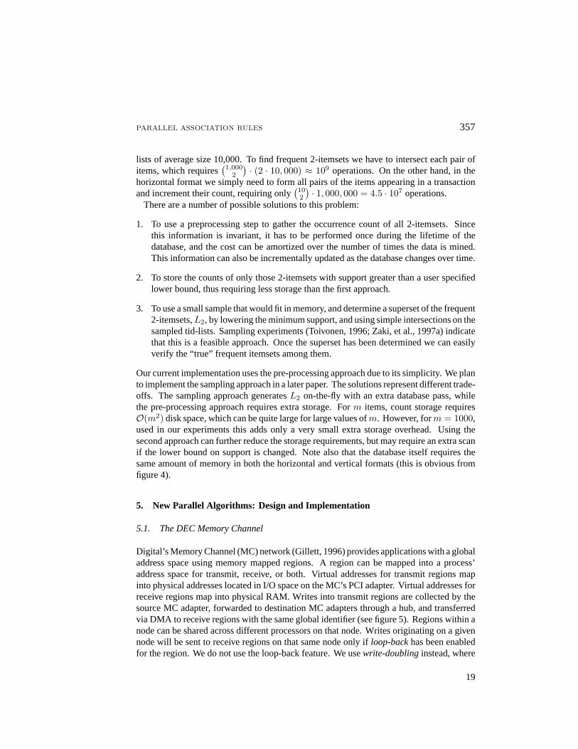
Digital’s Memory Channel (MC) network (Gillett, 1996) provides applications with a globaladdress space using memory mapped regions. A region can be mapped into a process’address space for transmit, receive, or both. Virtual addresses for transmit regions mapinto physical addresses located in I/O space on the MC’s PCI adapter. Virtual addresses forreceive regions map into physical RAM. Writes into transmit regions are collected by thesource MC adapter, forwarded to destination MC adapters through a hub, and transferredvia DMA to receive regions with the same global identifier (see figure 5). Regions within anode can be shared across different processors on that node. Writes originating on a givennode will be sent to receive regions on that same node only ifloop-backhas been enabledfor the region. We do not use the loop-back feature. We usewrite-doublinginstead, where
19
358 ZAKI, PARTHASARATHY, OGIHARA AND LI
Figure 5. Memory Channel space. The lined region is mapped for both transmit and receive on node 1 and forreceive on node 2. The gray region is mapped for receive on node 1 and for transmit on node 2.
each processor writes to its receive region and then to its transmit region, so that processeson a host can see modification made by other processes on the same host. Though we paythe cost of double writing, we reduce the amount of messages to the hub.
In our system unicast and multicast process-to-process writes have a latency of 5.2µs,with per-link transfer bandwidths of 30 MB/s. MC peak aggregate bandwidth is also about32 MB/s. Memory Channel guarantees write ordering and local cache coherence. Twowrites issued to the same transmit region (even on different nodes) will appear in the sameorder in every receive region. When a write appears in a receive region it invalidates anylocally cached copies of its line.
5.2. Initial Database Partitioning
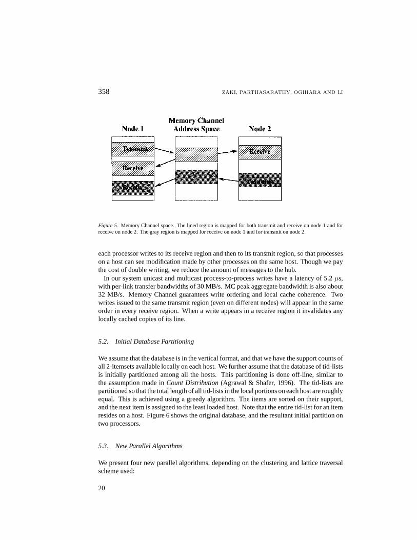
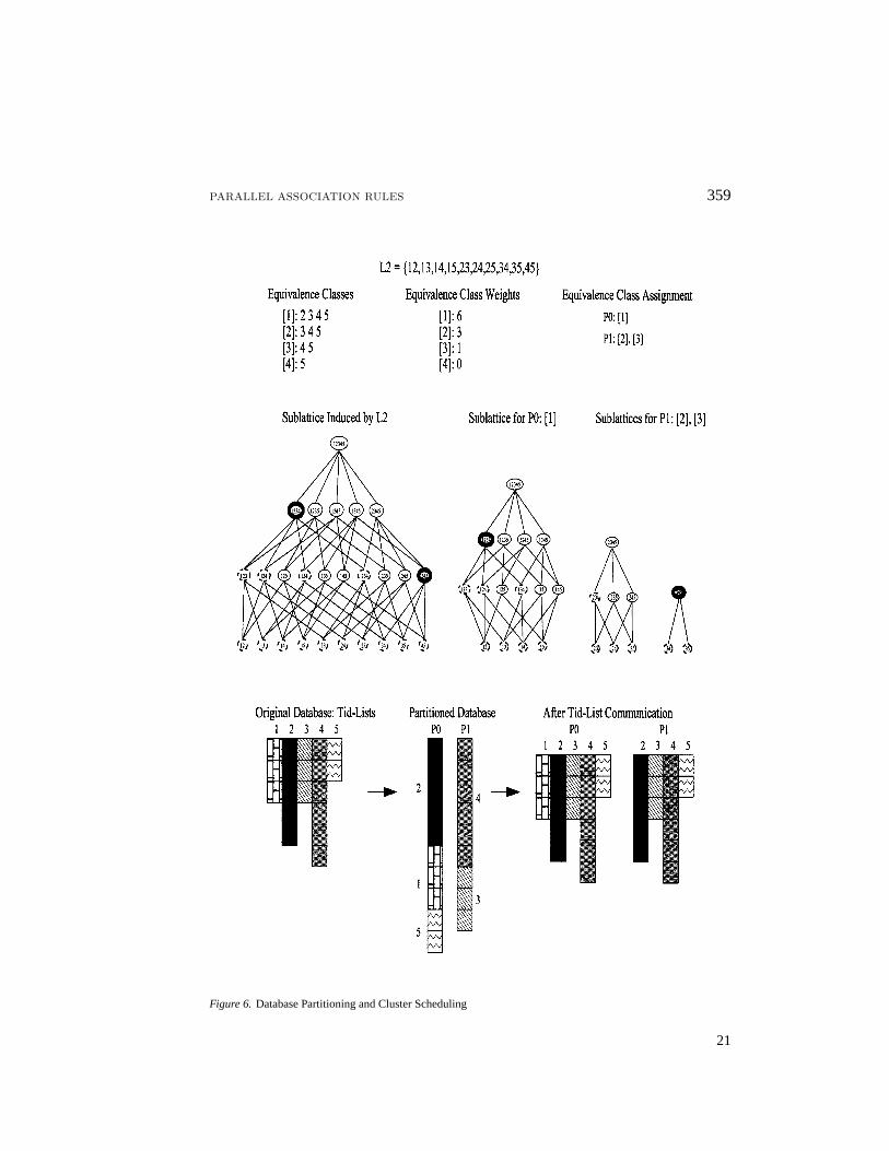
We assume that the database is in the vertical format, and that we have the support counts ofall 2-itemsets available locally on each host. We further assume that the database of tid-listsis initially partitioned among all the hosts. This partitioning is done off-line, similar tothe assumption made inCount Distribution(Agrawal & Shafer, 1996). The tid-lists arepartitioned so that the total length of all tid-lists in the local portions on each host are roughlyequal. This is achieved using a greedy algorithm. The items are sorted on their support,and the next item is assigned to the least loaded host. Note that the entire tid-list for an itemresides on a host. Figure 6 shows the original database, and the resultant initial partition ontwo processors.
5.3. New Parallel Algorithms
We present four new parallel algorithms, depending on the clustering and lattice traversalscheme used:
20
PARALLEL ASSOCIATION RULES 359
Figure 6. Database Partitioning and Cluster Scheduling
21
360 ZAKI, PARTHASARATHY, OGIHARA AND LI
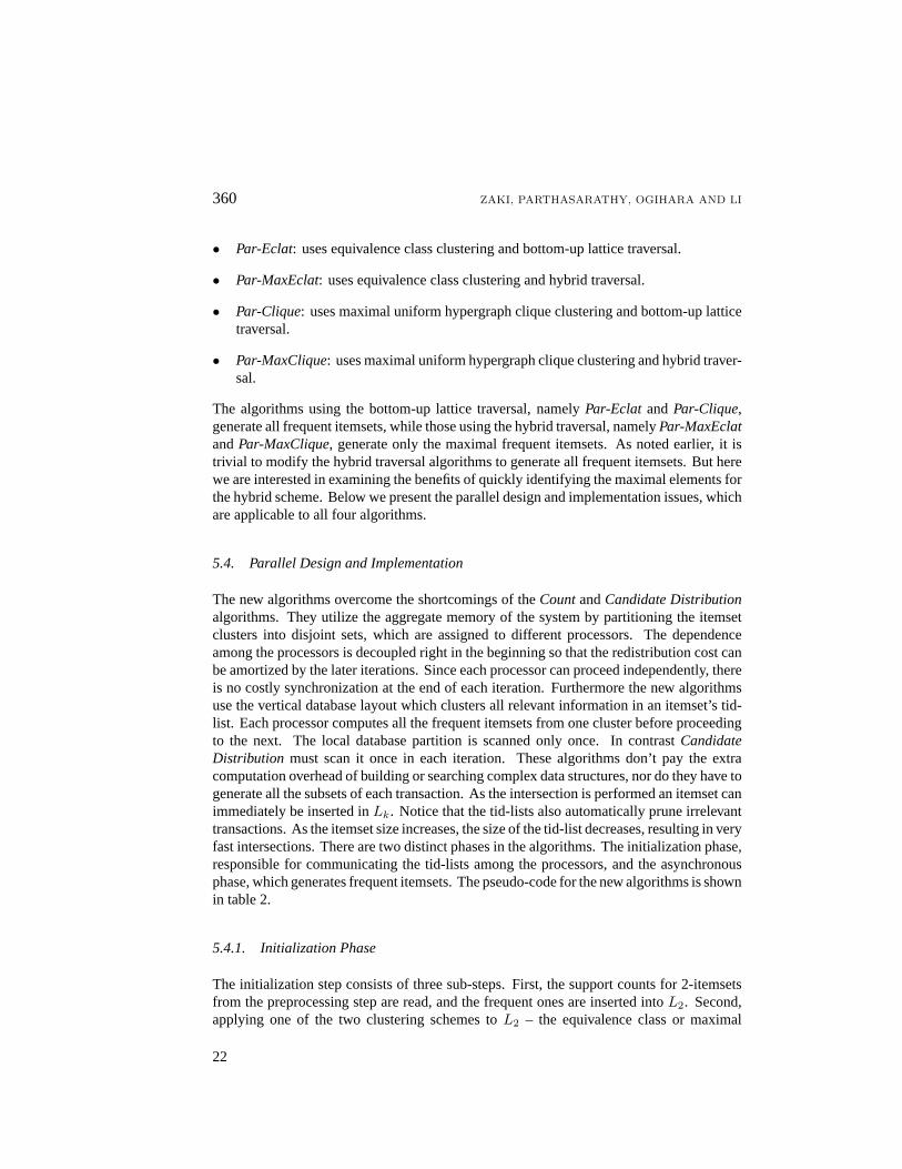
• Par-Eclat: uses equivalence class clustering and bottom-up lattice traversal.
• Par-MaxEclat: uses equivalence class clustering and hybrid traversal.
• Par-Clique: uses maximal uniform hypergraph clique clustering and bottom-up latticetraversal.
• Par-MaxClique: uses maximal uniform hypergraph clique clustering and hybrid traver-sal.
The algorithms using the bottom-up lattice traversal, namelyPar-Eclat andPar-Clique,generate all frequent itemsets, while those using the hybrid traversal, namelyPar-MaxEclatandPar-MaxClique, generate only the maximal frequent itemsets. As noted earlier, it istrivial to modify the hybrid traversal algorithms to generate all frequent itemsets. But herewe are interested in examining the benefits of quickly identifying the maximal elements forthe hybrid scheme. Below we present the parallel design and implementation issues, whichare applicable to all four algorithms.
5.4. Parallel Design and Implementation
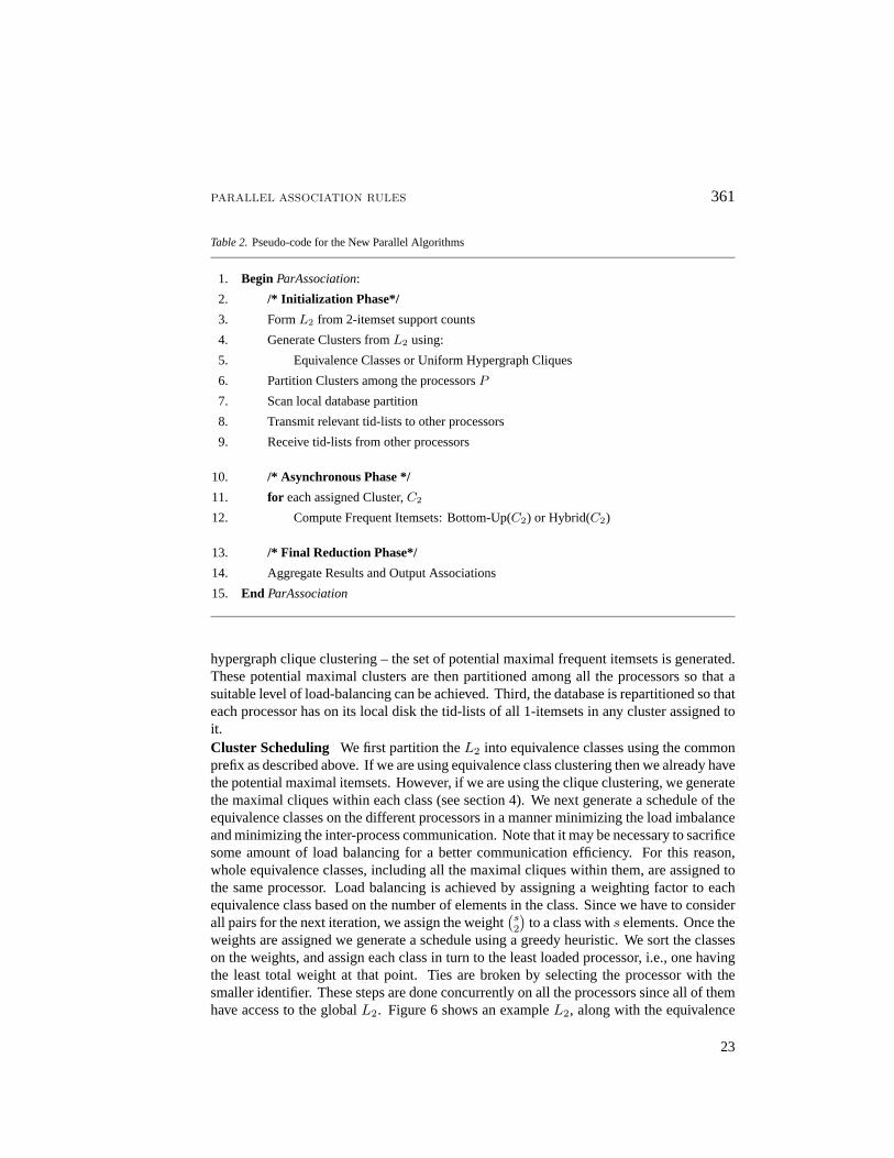
The new algorithms overcome the shortcomings of theCountandCandidate Distributionalgorithms. They utilize the aggregate memory of the system by partitioning the itemsetclusters into disjoint sets, which are assigned to different processors. The dependenceamong the processors is decoupled right in the beginning so that the redistribution cost canbe amortized by the later iterations. Since each processor can proceed independently, thereis no costly synchronization at the end of each iteration. Furthermore the new algorithmsuse the vertical database layout which clusters all relevant information in an itemset’s tid-list. Each processor computes all the frequent itemsets from one cluster before proceedingto the next. The local database partition is scanned only once. In contrastCandidateDistribution must scan it once in each iteration. These algorithms don’t pay the extracomputation overhead of building or searching complex data structures, nor do they have togenerate all the subsets of each transaction. As the intersection is performed an itemset canimmediately be inserted inLk. Notice that the tid-lists also automatically prune irrelevanttransactions. As the itemset size increases, the size of the tid-list decreases, resulting in veryfast intersections. There are two distinct phases in the algorithms. The initialization phase,responsible for communicating the tid-lists among the processors, and the asynchronousphase, which generates frequent itemsets. The pseudo-code for the new algorithms is shownin table 2.
5.4.1. Initialization Phase
The initialization step consists of three sub-steps. First, the support counts for 2-itemsetsfrom the preprocessing step are read, and the frequent ones are inserted intoL2. Second,applying one of the two clustering schemes toL2 – the equivalence class or maximal
22
PARALLEL ASSOCIATION RULES 361
Table 2.Pseudo-code for the New Parallel Algorithms
1. BeginParAssociation:
2. /* Initialization Phase*/
3. FormL2 from 2-itemset support counts
4. Generate Clusters fromL2 using:
5. Equivalence Classes or Uniform Hypergraph Cliques
6. Partition Clusters among the processorsP
7. Scan local database partition
8. Transmit relevant tid-lists to other processors
9. Receive tid-lists from other processors
10. /* Asynchronous Phase */
11. for each assigned Cluster,C2
12. Compute Frequent Itemsets: Bottom-Up(C2) or Hybrid(C2)
13. /* Final Reduction Phase*/
14. Aggregate Results and Output Associations
15. End ParAssociation
hypergraph clique clustering – the set of potential maximal frequent itemsets is generated.These potential maximal clusters are then partitioned among all the processors so that asuitable level of load-balancing can be achieved. Third, the database is repartitioned so thateach processor has on its local disk the tid-lists of all 1-itemsets in any cluster assigned toit.Cluster Scheduling We first partition theL2 into equivalence classes using the commonprefix as described above. If we are using equivalence class clustering then we already havethe potential maximal itemsets. However, if we are using the clique clustering, we generatethe maximal cliques within each class (see section 4). We next generate a schedule of theequivalence classes on the different processors in a manner minimizing the load imbalanceand minimizing the inter-process communication. Note that it may be necessary to sacrificesome amount of load balancing for a better communication efficiency. For this reason,whole equivalence classes, including all the maximal cliques within them, are assigned tothe same processor. Load balancing is achieved by assigning a weighting factor to eachequivalence class based on the number of elements in the class. Since we have to considerall pairs for the next iteration, we assign the weight
(s2
)to a class withs elements. Once the
weights are assigned we generate a schedule using a greedy heuristic. We sort the classeson the weights, and assign each class in turn to the least loaded processor, i.e., one havingthe least total weight at that point. Ties are broken by selecting the processor with thesmaller identifier. These steps are done concurrently on all the processors since all of themhave access to the globalL2. Figure 6 shows an exampleL2, along with the equivalence
23
362 ZAKI, PARTHASARATHY, OGIHARA AND LI
classes, their weights, and the assignment of the classes on two processors. Notice how anentire sublattice induced by a given class is assigned to a single processor. This leads tobetter load balancing, even though the partitioning may introduce extra computation. Forexample, if234 were not frequent, then1234 cannot be frequent either. But since thesebelong to different equivalence classes assigned to different processors, this informationis not used. Although the size of a class gives a good indication of the amount of work,better heuristics for generating the weights are possible. For example, if we could betterestimate the number of frequent itemsets that could be derived from an equivalence class wecould use this estimation as our weight. We believe that decoupling processor performanceright in the beginning holds promise, even though it may cause some load imbalance, sincethe repartitioning cost can be amortized over later iterations. Deriving better heuristics forscheduling the clusters, which minimize the load imbalance as well as communication, ispart of ongoing research.Tid-list Communication Once the clusters have been partitioned among the processorseach processor has to exchange information with every other processor to read the non-localtid-lists over the Memory Channel network. To minimize communication, and being awareof the fact that in our configuration there is only one local disk per host (recall that our clusterhas 8 hosts, with 4 processors per host), only the hosts take part in the tid-list exchange.Additional processes on each of the 8 hosts are spawned only in the asynchronous phase. Toaccomplish the inter-process tid-list communication, each processor scans the item tid-listsin its local database partition and writes it to a transmit region which is mapped for receiveon other processors. The other processors extract the tid-list from the receive region ifit belongs to any cluster assigned to them. For example, figure 6 shows the initial localdatabase on two hosts, and the final local database after the tid-list communication.
5.4.2. Asynchronous Phase
At the end of the initialization step, the relevant tid-lists are available locally on each host,thus each processor can independently generate the frequent itemsets from its assignedmaximal clusters, eliminating the need for synchronization with other processors. Eachcluster is processed in its entirety before moving on to the next cluster. This step involvesscanning the local database partition only once. We thus benefit from huge I/O savings.Since each cluster induces a sublattice, depending on the algorithm, we either use a bottom-up traversal to generate all frequent itemsets, or we use the hybrid traversal to generateonly the maximal frequent itemsets. The pseudo-code of the two lattice traversal schemesis shown in table 3.
Note that initially we only have the tid-lists for 1-itemsets stored locally on disk. Usingthese, the tid-lists for the 2-itemset clusters are generated, and since these clusters aregenerally small the resulting tid-lists can be kept in memory. In the bottom-up approach,the tid-lists for 2-itemsets clusters are intersected to generate 3-itemsets. If the cardinality ofthe resulting tid-list exceeds the minimum support, the new itemset is inserted inL3. Thenwe split the resulting frequent 3-itemsets,L3 into equivalence classes based on commonprefixes of length 2. All pairs of 3-itemsets within an equivalence class are intersected todetermineL4, and so on till all frequent itemsets are found. OnceLk has been determined,
24
PARALLEL ASSOCIATION RULES 363
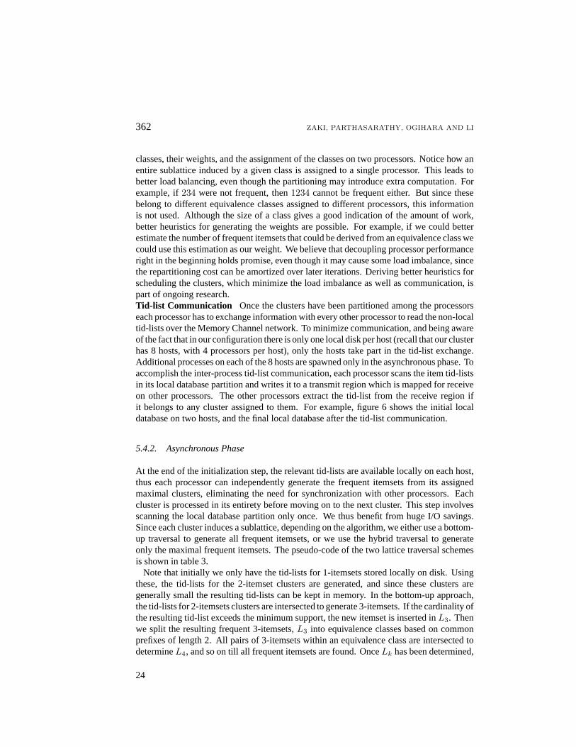
Table 3.Pseudo-code for Bottom-up and Hybrid Traversal
1. Input: Ck = {I1, .., In}, equivalence
2. class or maximal clique
3. clustering of k-itemsets.
4. Output: Frequent itemsets∈ Ck
5. Bottom-Up(Ck):
6. for all Ii ∈ Ck do
7. Ck+1 = ∅;8. for all Ij ∈ Ck, i < j do
9. N = (Ii ∩ Ij );10. if N.sup≥ minsupthen
11. Ck+1 = Ck+1 ∪ {N};12. end;
13. if Ck+1 6= ∅ then
14. Bottom-Up(Ck+1);
15. end;
1. Hybrid(C2):
2. /* Top-Down Phase */
3. N = I1; S1 = {I1};4. for all Ii ∈ C2, i > 1 do
5. N = (N∩ Ii);6. if N.sup≥ minsupthen
7. S1 = S1 ∪ {Ii};8. elsebreak;
9. end;
10. S2 = C2 − S1;
11. /* Bottom-Up Phase */
12. for all Ii ∈ S2,do
13. C3 = {(Ii ∩Xj)|Xj ∈ S1};14. S1 = S1 ∪ {Ii};15. if C3 6= ∅ then Bottom-Up(C3);
16. end;
we can deleteLk−1. We thus need main memory space only for the itemsets inLk−1 withinone maximal cluster. For the top-down phase of the hybrid traversal only the maximalelement seen so far needs to be memory-resident, along with the itemsets not yet seen. Thenew algorithms are therefore main memory space efficient. Experimental results on thememory usage of these algorithms are presented in the next section.
Pruning Candidates Recall that bothCountandCandidate Distributionuse a pruningstep to eliminate unnecessary candidates. This step is essential in those algorithms to reducethe size of the hash tree. Smaller trees lead to faster support counting, since each subset ofa transaction is tested against the tree. However, with the vertical database layout we foundthe pruning step to be of little or no help. This can be attributed to several factors. First, thereis additional space and computation overhead in constructing and searching hash tables.This is also likely to degrade locality. Second, there is extra overhead in generating all thesubsets of a candidate. Third, there is extra communication overhead in communicatingthe frequent itemsets in each iteration, even though it may happen asynchronously. Fourth,because the average size of tid-lists decreases as the itemsets size increases, intersectionscan be performed very quickly with the short-circuit mechanism.
At the end of the asynchronous phase we accumulate all the results from each processorand print them out.
25
364 ZAKI, PARTHASARATHY, OGIHARA AND LI
5.5. Salient Features of the New Algorithms
In this section we will recapitulate the salient features of our proposed algorithms, contrast-ing them againstCountandCandidate Distribution. Our algorithms differ in the followingrespect:
• Unlike Count Distribution, they utilize the aggregate memory of the parallel system bypartitioning the candidate itemsets among the processors using the itemset clusteringschemes.
• They decouple the processors right in the beginning by repartitioning the database, sothat each processor can compute the frequent itemsets independently. This eliminatesthe need for communicating the frequent itemsets at the end of each iteration.
• They use the vertical database layout which clusters the transactions containing anitemset into tid-lists. Using this layout enables our algorithms to scan the local databasepartition only two times on each processor. The first scan for communicating the tid-lists, and the second for obtaining the frequent itemsets. In contrast, bothCountandCandidate Distributionscan the database multiple times – once during each iteration.
• To compute frequent itemsets, they performs simple intersections on two tid-lists.There is no extra overhead associated with building and searching complex hash treedata structures. Such complicated hash structures also suffer from poor cache locality(Parthasarathy, Zaki, & Li, 1997). In our algorithms, all the available memory is utilizedto keep tid-lists in memory which results in good locality. As larger itemsets are gener-ated the size of tid-lists decreases, resulting in very fast intersections. Short-circuitingthe join based on minimum support is also used to speed this step.
• Our algorithms avoid the overhead of generating all the subsets of a transaction andchecking them against the candidate hash tree during support counting.
6. Experimental Evaluation
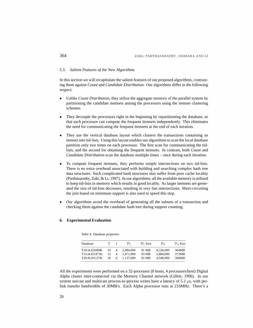
Table 4.Database properties
Database T I D1 D1 Size D4 D4 Size
T10.I4.D2084K 10 4 2,084,000 91 MB 8,336,000 364MBT15.I4.D1471K 15 4 1,471,000 93 MB 5,884,000 372MBT20.I6.D1137K 20 6 1,137,000 92 MB 4,548,000 368MB
All the experiments were performed on a 32-processor (8 hosts, 4 processors/host) DigitalAlpha cluster inter-connected via the Memory Channel network (Gillett, 1996). In oursystem unicast and multicast process-to-process writes have a latency of 5.2µs, with per-link transfer bandwidths of 30MB/s. Each Alpha processor runs at 233MHz. There’s a
26
PARALLEL ASSOCIATION RULES 365
total of 256MB of main memory per host (shared among the 4 processors on that host).Each host also has a 2GB local disk attached to it, out of which less than 500MB wasavailable to us. All the partitioned databases reside on the local disks of each processor. Weused different synthetic databases, generated using the procedure described in (Agrawal &Srikant, 1994). These have been used as benchmark databases for many association rulesalgorithms (Agrawal & Srikant, 1994; Holsheimer, et al., 1995; Park, Chen, & Yu, 1995a;Savasere, Omiecinski, & Navathe, 1995; Agrawal, et al., 1996). Table 4 shows the databasesused and their properties. The number of transactions is denoted asDr, wherer is thereplication factor. Forr = 1, all the databases are roughly 90MB in size. Except forthe sizeup experiments, all results shown are on databases with a replication factor ofr = 4 (≈360MB). We could not go beyond a replication factor of 6 (used in sizeupexperiments) since the repartitioned database would become too large to fit on disk. Theaverage transaction size is denoted as|T |, and the average maximal potentially frequentitemset size as|I|. The number of maximal potentially frequent itemsets|L| = 2000, andthe number of itemsN = 1000. We refer the reader to (Agrawal & Srikant, 1994) for moredetail on the database generation. All the experiments were performed with a minimumsupport value of 0.25%. For a fair comparison, all algorithms discover frequentk-itemsetsfor k ≥ 3, using the supports for the 2-itemsets from the preprocessing step.
6.1. Performance Comparison
H1.P1.T1 H1.P2.T2 H2.P1.T2 H1.P4.T4 H2.P2.T4 H4.P1.T4 H2.P4.T8 H4.P2.T8 H8.P1.T8 H4.P4.T16 H8.P2.T16 H8.P4.T320
200
400
600
800
1000
1200
To
tal E
xe
cu
tio
n T
ime
(se
c)
Count Distribution
Par-Eclat
T10.I4.D2084K
H1.P1.T1 H1.P2.T2 H2.P1.T2 H1.P4.T4 H2.P2.T4 H4.P1.T4 H2.P4.T8 H4.P2.T8 H8.P1.T8 H4.P4.T16 H8.P2.T16 H8.P4.T320
20
40
60
80
100
120
140
160
180
200
To
tal E
xe
cu
tio
n T
ime
(se
c)
Par-Eclat
Par-Clique
Par-MaxEclat
Par-MaxClique
T10.I4.D2084K
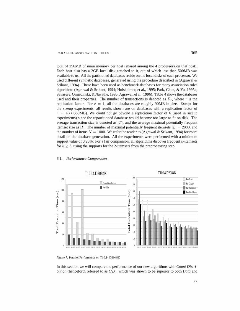
Figure 7. Parallel Performance on T10.I4.D2048K
In this section we will compare the performance of our new algorithms withCount Distri-bution (henceforth referred to asCD), which was shown to be superior to bothData and
27
366 ZAKI, PARTHASARATHY, OGIHARA AND LI
H1.P1.T1 H1.P2.T2 H2.P1.T2 H1.P4.T4 H2.P2.T4 H4.P1.T4 H2.P4.T8 H4.P2.T8 H8.P1.T8 H4.P4.T16 H8.P2.T16 H8.P4.T320
200
400
600
800
1000
1200
1400
1600
1800
2000
To
tal E
xe
cu
tio
n T
ime
(se
c)
Count Distribution
Par-Eclat
T15.I4.D1471K
H1.P1.T1 H1.P2.T2 H2.P1.T2 H1.P4.T4 H2.P2.T4 H4.P1.T4 H2.P4.T8 H4.P2.T8 H8.P1.T8 H4.P4.T16 H8.P2.T16 H8.P4.T320
50
100
150
200
250
300
350
400
450
To
tal E
xe
cu
tio
n T
ime
(se
c)
Par-Eclat
Par-Clique
Par-MaxEclat
Par-MaxClique
T15.I4.D1471K
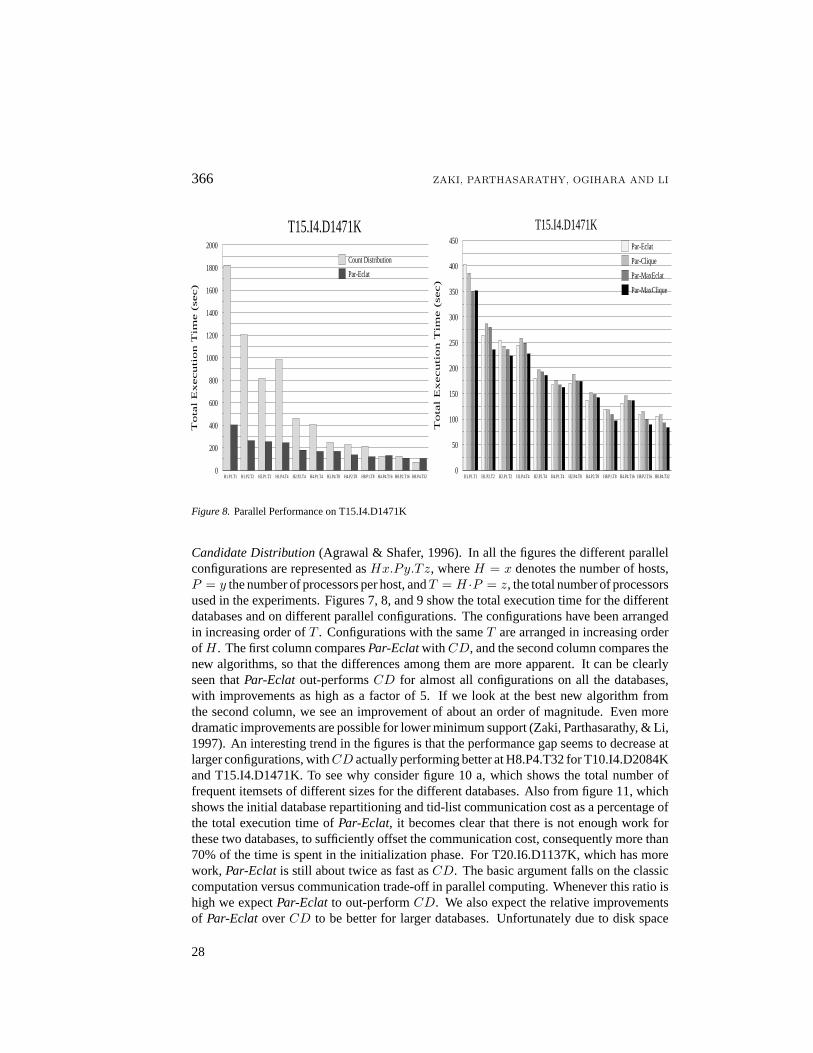
Figure 8. Parallel Performance on T15.I4.D1471K
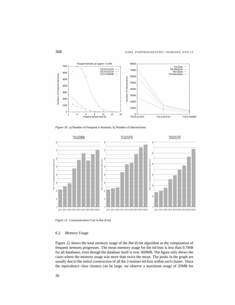
Candidate Distribution(Agrawal & Shafer, 1996). In all the figures the different parallelconfigurations are represented asHx.Py.Tz, whereH = x denotes the number of hosts,P = y the number of processors per host, andT = H ·P = z, the total number of processorsused in the experiments. Figures 7, 8, and 9 show the total execution time for the differentdatabases and on different parallel configurations. The configurations have been arrangedin increasing order ofT . Configurations with the sameT are arranged in increasing orderofH. The first column comparesPar-EclatwithCD, and the second column compares thenew algorithms, so that the differences among them are more apparent. It can be clearlyseen thatPar-Eclat out-performsCD for almost all configurations on all the databases,with improvements as high as a factor of 5. If we look at the best new algorithm fromthe second column, we see an improvement of about an order of magnitude. Even moredramatic improvements are possible for lower minimum support (Zaki, Parthasarathy, & Li,1997). An interesting trend in the figures is that the performance gap seems to decrease atlarger configurations, withCD actually performing better at H8.P4.T32 for T10.I4.D2084Kand T15.I4.D1471K. To see why consider figure 10 a, which shows the total number offrequent itemsets of different sizes for the different databases. Also from figure 11, whichshows the initial database repartitioning and tid-list communication cost as a percentage ofthe total execution time ofPar-Eclat, it becomes clear that there is not enough work forthese two databases, to sufficiently offset the communication cost, consequently more than70% of the time is spent in the initialization phase. For T20.I6.D1137K, which has morework, Par-Eclat is still about twice as fast asCD. The basic argument falls on the classiccomputation versus communication trade-off in parallel computing. Whenever this ratio ishigh we expectPar-Eclat to out-performCD. We also expect the relative improvementsof Par-Eclat overCD to be better for larger databases. Unfortunately due to disk space
28
PARALLEL ASSOCIATION RULES 367
constraints we were not able to test the algorithms on larger databases. In all except theH = 1 configurations, the local database partition is less than available memory. ForCD,the entire database would be cached after the first scan. The performance ofCD is thus abest case scenario for it since the results do not include the “real” hitCD would have takenfrom multiple disk scans. As mentioned in section 5.5,Par-Eclatwas designed to scan thedatabase only once during frequent itemset computation.
H1.P1.T1 H1.P2.T2 H2.P1.T2 H1.P4.T4 H2.P2.T4 H4.P1.T4 H2.P4.T8 H4.P2.T8 H8.P1.T8 H4.P4.T16 H8.P2.T16 H8.P4.T320
1000
2000
3000
4000
5000
6000
To
tal E
xe
cu
tio
n T
ime
(se
c)
Count Distribution
Par-Eclat
T20.I6.D1137K
H1.P1.T1 H1.P2.T2 H2.P1.T2 H1.P4.T4 H2.P2.T4 H4.P1.T4 H2.P4.T8 H4.P2.T8 H8.P1.T8 H4.P4.T16 H8.P2.T16 H8.P4.T320
200
400
600
800
1000
1200
To
tal E
xe
cu
tio
n T
ime
(se
c)
Par-Eclat
Par-Clique
Par-MaxEclat
Par-MaxClique
T20.I6.D1137K
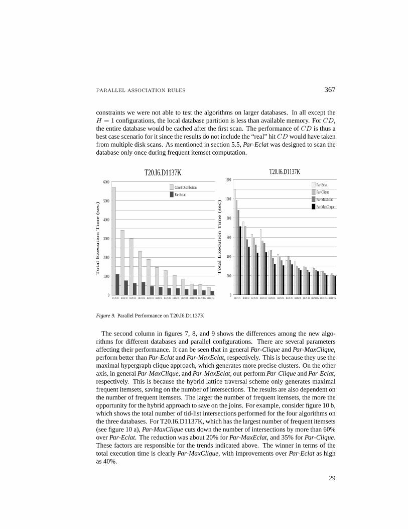
Figure 9. Parallel Performance on T20.I6.D1137K
The second column in figures 7, 8, and 9 shows the differences among the new algo-rithms for different databases and parallel configurations. There are several parametersaffecting their performance. It can be seen that in generalPar-CliqueandPar-MaxClique,perform better thanPar-EclatandPar-MaxEclat, respectively. This is because they use themaximal hypergraph clique approach, which generates more precise clusters. On the otheraxis, in generalPar-MaxClique, andPar-MaxEclat, out-performPar-CliqueandPar-Eclat,respectively. This is because the hybrid lattice traversal scheme only generates maximalfrequent itemsets, saving on the number of intersections. The results are also dependent onthe number of frequent itemsets. The larger the number of frequent itemsets, the more theopportunity for the hybrid approach to save on the joins. For example, consider figure 10 b,which shows the total number of tid-list intersections performed for the four algorithms onthe three databases. For T20.I6.D1137K, which has the largest number of frequent itemsets(see figure 10 a),Par-MaxCliquecuts down the number of intersections by more than 60%overPar-Eclat. The reduction was about 20% forPar-MaxEclat, and 35% forPar-Clique.These factors are responsible for the trends indicated above. The winner in terms of thetotal execution time is clearlyPar-MaxClique, with improvements overPar-Eclatas highas 40%.
29
368 ZAKI, PARTHASARATHY, OGIHARA AND LI
0
1000
2000
3000
4000
5000
6000
7000
2 4 6 8 10 12 14
Num
ber
of F
requent Item
sets
Frequent Itemset Size (k)
Frequent Itemsets at Support = 0.25%
T20.I6.D1137KT15.I4.D1471KT10.I4.D2084K
0
10000
20000
30000
40000
50000
60000
70000
80000
T20.I6.D1137K T15.I4.D1471K T10.I4.D2084K
Num
ber
of In
ters
ections
Par-EclatPar-MaxEclat
Par-CliquePar-MaxClique
Figure 10.a) Number of Frequentk-Itemsets; b) Number of Intersections
H2.P1.T2 H2.P2.T4 H2.P4.T8 H4.P1.T4 H4.P2.T8 H4.P4.T16 H8.P1.T8 H8.P2.T16 H8.P4.T320
10
20
30
40
50
60
70
80
% C
om
mu
nic
atio
n
T10.I4.D2084K
H2.P1.T2 H2.P2.T4 H2.P4.T4 H4.P1.T4 H4.P2.T8 H4.P4.T16 H8.P1.T8 H8.P2.T16 H8.P4.T320
10
20
30
40
50
60
70
80
% C
om
mu
nic
atio
n
T15.I4.D1471K
H2.P1.T2 H2.P2.T4 H2.P4.T8 H4.P1.T4 H4.P2.T8 H4.P4.T16 H8.P1.T8 H8.P2.T16 H8.P4.T320
10
20
30
40
50
60
% C
om
mu
nic
atio
n
T20.I6.D1137K
Figure 11.Communication Cost inPar-Eclat
6.2. Memory Usage
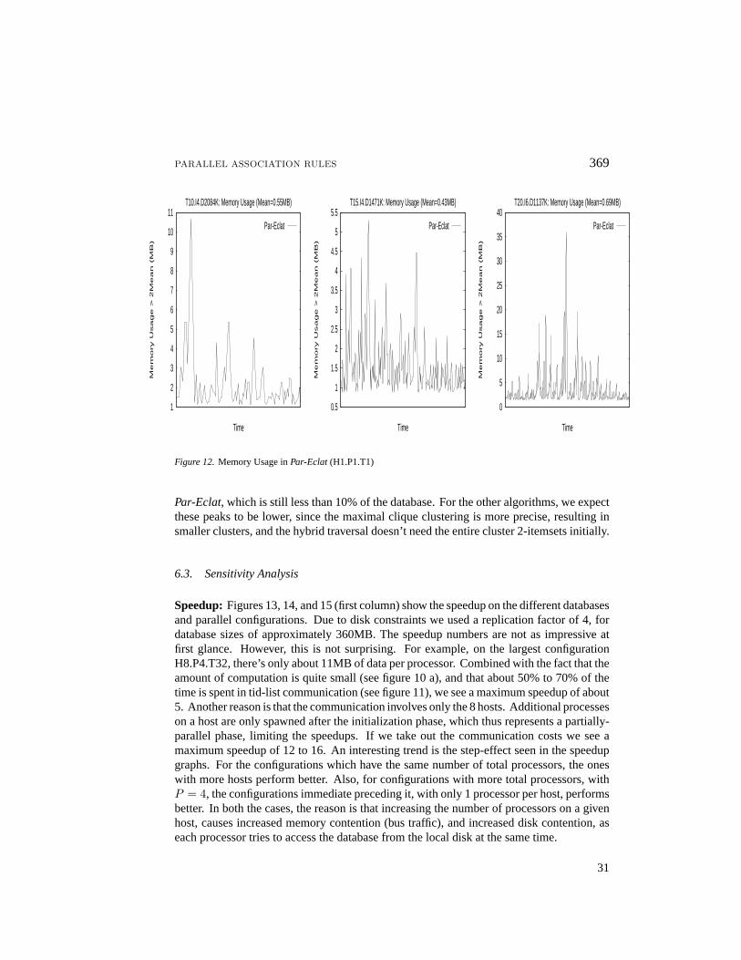
Figure 12 shows the total memory usage of thePar-Eclatalgorithm as the computation offrequent itemsets progresses. The mean memory usage for the tid-lists is less than 0.7MBfor all databases, even though the database itself is over 360MB. The figure only shows thecases where the memory usage was more than twice the mean. The peaks in the graph areusually due to the initial construction of all the 2-itemset tid-lists within each cluster. Sincethe equivalence class clusters can be large, we observe a maximum usage of 35MB for
30
PARALLEL ASSOCIATION RULES 369
1
2
3
4
5
6
7
8
9
10
11
Me
mo
ry U
sa
ge
>
2
Me
an
(M
B)
Time
T10.I4.D2084K: Memory Usage (Mean=0.55MB)
Par-Eclat
0.5
1
1.5
2
2.5
3
3.5
4
4.5
5
5.5
Me
mo
ry U
sa
ge
>
2
Me
an
(M
B)
Time
T15.I4.D1471K: Memory Usage (Mean=0.43MB)
Par-Eclat
0
5
10
15
20
25
30
35
40
Me
mo
ry U
sa
ge
>
2
Me
an
(M
B)
Time
T20.I6.D1137K: Memory Usage (Mean=0.69MB)
Par-Eclat
Figure 12.Memory Usage inPar-Eclat(H1.P1.T1)
Par-Eclat, which is still less than 10% of the database. For the other algorithms, we expectthese peaks to be lower, since the maximal clique clustering is more precise, resulting insmaller clusters, and the hybrid traversal doesn’t need the entire cluster 2-itemsets initially.
6.3. Sensitivity Analysis
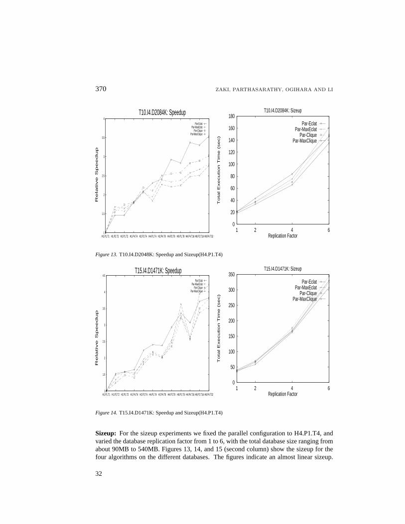
Speedup:Figures 13, 14, and 15 (first column) show the speedup on the different databasesand parallel configurations. Due to disk constraints we used a replication factor of 4, fordatabase sizes of approximately 360MB. The speedup numbers are not as impressive atfirst glance. However, this is not surprising. For example, on the largest configurationH8.P4.T32, there’s only about 11MB of data per processor. Combined with the fact that theamount of computation is quite small (see figure 10 a), and that about 50% to 70% of thetime is spent in tid-list communication (see figure 11), we see a maximum speedup of about5. Another reason is that the communication involves only the 8 hosts. Additional processeson a host are only spawned after the initialization phase, which thus represents a partially-parallel phase, limiting the speedups. If we take out the communication costs we see amaximum speedup of 12 to 16. An interesting trend is the step-effect seen in the speedupgraphs. For the configurations which have the same number of total processors, the oneswith more hosts perform better. Also, for configurations with more total processors, withP = 4, the configurations immediate preceding it, with only 1 processor per host, performsbetter. In both the cases, the reason is that increasing the number of processors on a givenhost, causes increased memory contention (bus traffic), and increased disk contention, aseach processor tries to access the database from the local disk at the same time.
31
370 ZAKI, PARTHASARATHY, OGIHARA AND LI
1
1.5
2
2.5
3
3.5
4
H1.P1.T1 H1.P2.T2 H2.P1.T2 H1.P4.T4 H2.P2.T4 H4.P1.T4 H2.P4.T8 H4.P2.T8 H8.P1.T8 H4.P4.T16 H8.P2.T16 H8.P4.T32
Re
lative
Sp
ee
du
p
T10.I4.D2084K: SpeedupPar-Eclat
Par-MaxEclatPar-Clique
Par-MaxClique
0
20
40
60
80
100
120
140
160
180
1 2 4 6
Tota
l E
xecution T
ime (
sec)
Replication Factor
T10.I4.D2084K: Sizeup
Par-EclatPar-MaxEclat
Par-CliquePar-MaxClique
Figure 13.T10.I4.D2048K: Speedup and Sizeup(H4.P1.T4)
1
1.5
2
2.5
3
3.5
4
4.5
H1.P1.T1 H1.P2.T2 H2.P1.T2 H1.P4.T4 H2.P2.T4 H4.P1.T4 H2.P4.T8 H4.P2.T8 H8.P1.T8 H4.P4.T16 H8.P2.T16 H8.P4.T32
Re
lative
Sp
ee
du
p
T15.I4.D1471K: SpeedupPar-Eclat
Par-MaxEclatPar-Clique
Par-MaxClique
0
50
100
150
200
250
300
350
1 2 4 6
Tota
l E
xecution T
ime (
sec)
Replication Factor
T15.I4.D1471K: Sizeup
Par-EclatPar-MaxEclat
Par-CliquePar-MaxClique
Figure 14.T15.I4.D1471K: Speedup and Sizeup(H4.P1.T4)
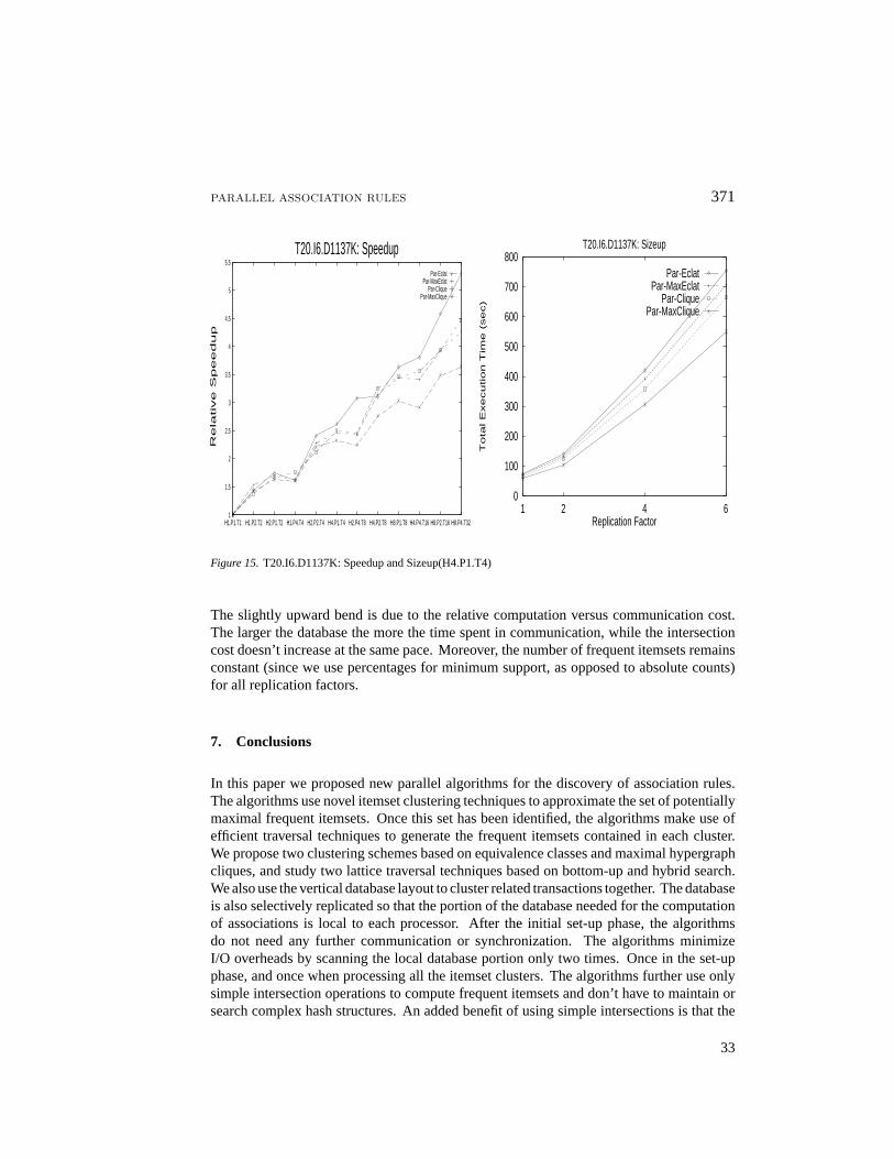
Sizeup: For the sizeup experiments we fixed the parallel configuration to H4.P1.T4, andvaried the database replication factor from 1 to 6, with the total database size ranging fromabout 90MB to 540MB. Figures 13, 14, and 15 (second column) show the sizeup for thefour algorithms on the different databases. The figures indicate an almost linear sizeup.
32
PARALLEL ASSOCIATION RULES 371
1
1.5
2
2.5
3
3.5
4
4.5
5
5.5
H1.P1.T1 H1.P2.T2 H2.P1.T2 H1.P4.T4 H2.P2.T4 H4.P1.T4 H2.P4.T8 H4.P2.T8 H8.P1.T8 H4.P4.T16 H8.P2.T16 H8.P4.T32
Re
lative
Sp
ee
du
p
T20.I6.D1137K: SpeedupPar-Eclat
Par-MaxEclatPar-Clique
Par-MaxClique
0
100
200
300
400
500
600
700
800
1 2 4 6
Tota
l E
xecution T
ime (
sec)
Replication Factor
T20.I6.D1137K: Sizeup
Par-EclatPar-MaxEclat
Par-CliquePar-MaxClique
Figure 15.T20.I6.D1137K: Speedup and Sizeup(H4.P1.T4)
The slightly upward bend is due to the relative computation versus communication cost.The larger the database the more the time spent in communication, while the intersectioncost doesn’t increase at the same pace. Moreover, the number of frequent itemsets remainsconstant (since we use percentages for minimum support, as opposed to absolute counts)for all replication factors.
7. Conclusions
In this paper we proposed new parallel algorithms for the discovery of association rules.The algorithms use novel itemset clustering techniques to approximate the set of potentiallymaximal frequent itemsets. Once this set has been identified, the algorithms make use ofefficient traversal techniques to generate the frequent itemsets contained in each cluster.We propose two clustering schemes based on equivalence classes and maximal hypergraphcliques, and study two lattice traversal techniques based on bottom-up and hybrid search.We also use the vertical database layout to cluster related transactions together. The databaseis also selectively replicated so that the portion of the database needed for the computationof associations is local to each processor. After the initial set-up phase, the algorithmsdo not need any further communication or synchronization. The algorithms minimizeI/O overheads by scanning the local database portion only two times. Once in the set-upphase, and once when processing all the itemset clusters. The algorithms further use onlysimple intersection operations to compute frequent itemsets and don’t have to maintain orsearch complex hash structures. An added benefit of using simple intersections is that the
33
372 ZAKI, PARTHASARATHY, OGIHARA AND LI
algorithms we propose can be implemented directly on general purpose database systems(Holsheimer, et al., 1995; Houtsma & Swami, 1995).
Using the above techniques we presented four new algorithms. ThePar-Eclat (equiva-lence class, bottom-up search) andPar-Clique(maximal clique, bottom-up search) algo-rithms, discover all frequent itemsets, while thePar-MaxEclat(equivalence class, hybridsearch) andPar-MaxClique(maximal clique, hybrid search) discover the maximal frequentitemsets. We implemented the algorithms on a 32 processor DEC cluster interconnectedwith the DEC Memory Channel network, and compared it against a well known parallelalgorithmCount Distribution(Agrawal & Shafer, 1996). Experimental results indicate thata substantial performance improvement is obtained using our techniques.
Acknowledgments
This work was supported in part by an NSF Research Initiation Award (CCR-9409120) andARPA contract F19628-94-C-0057.
References
Agrawal, R., and Shafer, J. 1996. Parallel mining of association rules. InIEEE Trans. on Knowledge and DataEngg., 8(6):962–969.
Agrawal, R., and Srikant, R. 1994. Fast algorithms for mining association rules. In20th VLDB Conf.Agrawal, R.; Mannila, H.; Srikant, R.; Toivonen, H.; and Verkamo, A. I. 1996. Fast discovery of association
rules. In Fayyad, U., and et al., eds.,Advances in Knowledge Discovery and Data Mining. MIT Press.Agrawal, R.; Imielinski, T.; and Swami, A. 1993. Mining association rules between sets of items in large
databases. InACM SIGMOD Intl. Conf. Management of Data.Berge, C. 1989.Hypergraphs: Combinatorics of Finite Sets. North-Holland.Cheung, D.; Han, J.; Ng, V.; Fu, A.; and Fu, Y. 1996a. A fast distributed algorithm for mining association rules.
4th Intl. Conf. Parallel and Distributed Info. Systems.Cheung, D.; Ng, V.; Fu, A.; and Fu, Y. 1996b. Efficient mining of association rules in distributed databases. In
IEEE Trans. on Knowledge and Data Engg., 8(6):911–922.Fayyad, U.; Piatetsky-Shapiro, G.; and Smyth, P. 1996. The KDD process for extracting useful knowledge from
volumes of data. InCommunications of the ACM – Data Mining and Knowledge Discovery in Databases.Garey, M. R., and Johnson, D. S. 1979.Computers and Intractability: A Guide to the Theory of NP-Completeness.
W. H. Freeman and Co.Gillett, R. 1996. Memory channel: An optimized cluster interconnect. InIEEE Micro, 16(2).Han, E.-H.; Karypis, G.; and Kumar, V. 1997. Scalable parallel data mining for association rules. InACM
SIGMOD Conf. Management of Data.Holsheimer, M.; Kersten, M.; Mannila, H.; and Toivonen, H. 1995. A perspective on databases and data mining.
In 1st Intl. Conf. Knowledge Discovery and Data Mining.Houtsma, M., and Swami, A. 1995. Set-oriented mining of association rules in relational databases. In11th Intl.
Conf. Data Engineering.Mannila, H.; Toivonen, H.; and Verkamo, I. 1994. Efficient algorithms for discovering association rules. InAAAI
Wkshp. Knowledge Discovery in Databases.Park, J. S.; Chen, M.; and Yu, P. S. 1995a. An effective hash based algorithm for mining association rules. In
ACM SIGMOD Intl. Conf. Management of Data.Park, J. S.; Chen, M.; and Yu, P. S. 1995b. Efficient parallel data mining for association rules. InACM Intl. Conf.
Information and Knowledge Management.Parthasarathy, S.; Zaki, M. J.; and Li, W. 1997. Application driven memory placement for dynamic data structures.
Technical Report URCS TR 653, University of Rochester.
34
PARALLEL ASSOCIATION RULES 373
Savasere, A.; Omiecinski, E.; and Navathe, S. 1995. An efficient algorithm for mining association rules in largedatabases. In21st VLDB Conf.
Toivonen, H. 1996. Sampling large databases for association rules. In22nd VLDB Conf.Zaki, M. J.; Ogihara, M.; Parthasarathy, S.; and Li, W. 1996. Parallel data mining for association rules on
shared-memory multi-processors. InSupercomputing’96.Zaki, M. J.; Parthasarathy, S.; Li, W.; and Ogihara, M. 1997a. Evaluation of sampling for data mining of
association rules. In7th Intl. Wkshp. Research Issues in Data Engg.Zaki, M. J.; Parthasarathy, S.; Ogihara, M.; and Li, W. 1997b. New algorithms for fast discovery of association
rules. In3rd Intl. Conf. on Knowledge Discovery and Data Mining.Zaki, M. J.; Parthasarathy, S.; Ogihara, M.; and Li, W. 1997c. New algorithms for fast discovery of association
rules. Technical Report URCS TR 651, University of Rochester.Zaki, M. J.; Parthasarathy, S.; and Li, W. 1997. A localized algorithm for parallel association mining. In9th
ACM Symp. Parallel Algorithms and Architectures.
Mohammed J. Zaki is currently completing his Ph.D. in computer science at the University ofRochester. He received a M.S. in computer science from Rochester in 1995. His research interests fo-cus on developing efficient parallel algorithms for various data mining and knowledge discovery tasks.
Srinivasan Parthasarathyis currently a doctoral student at the University of Rochester. He receiveda M.S. degree in electrical engineering from the University of Cincinnati in 1994, and a M.S. degreein computer science from the University of Rochester in 1996. His research interests include paralleland distributed systems and data mining.
Mitsunori Ogihara (also known as Ogiwara) received Ph.D. in Information Sciences from TokyoInstitute of Technology in 1993. He is currently an assistant professor of computer science in theUniversity of Rochester. His research interests are computational complexity, DNA computing, anddata-mining.
Wei Li received his Ph.D. in computer science from Cornell University in 1993. He is currentlywith the Java Products Group in Oracle Corporation. Before that, he was an Assistant Professor atthe University of Rochester. His current technical interests include Java compilation, software fornetwork computing, and data mining.
35