Embed Size (px)
Citation preview

Parallel Clustering for Visualizing Large Scientific Line Data
Jishang Wei∗
University of California, Davis
Hongfeng Yu†
Sandia National Laboratories
Jacqueline H. Chen‡
Sandia National Laboratories
Kwan-Liu Ma§
University of California, Davis
ABSTRACT
Scientists often need to extract, visualize and analyze lines fromvast amounts of data to understand dynamic structures and inter-actions. The effectiveness of such a visual validation and analysisprocess mainly relies on a good strategy to categorize and visualizethe lines. However, the sheer size of line data produced by state-of-the-art scientific simulations poses great challenges to preparingthe data for visualization. In this paper, we present a parallelizationdesign of regression model-based clustering to categorize large linedata derived from detailed scientific simulations by leveraging thepower of heterogeneous computers. This parallel clustering methodemploys the Expectation Maximization algorithm to iteratively ap-proximate the optimal data partitioning. First, we use a sorted-balance algorithm to partition and distribute the lines with variouslengths among multiple compute nodes. During the following iter-ative clustering process, regression model parameters are recoveredbased on the local lines on each individual node, with only a fewinter-node message exchanges involved. Meanwhile, the workloadof regression model computing is well balanced across the nodes.The experimental results demonstrate that our approach can effec-tively categorize large line data in a scalable manner to conciselyconvey dynamic structures and interactions, leading to a visualiza-tion that captures salient features and suppresses visual clutter tofacilitate scientific exploration of large line data.
1 INTRODUCTION
Advanced computing and imaging techniques enables scientists tostudy problems of unprecedented complexity at high fidelity. Es-pecially, an advanced simulation can generate vast amounts of datafrom hundreds to thousands of time steps with tens of variables.From such large complex data, scientists often need to extract orderive line data to help understand dynamic structures and interac-tions hidden in the data. Typical examples of line data include whitematter fibers, time series curves, and vector field lines, which are ofgreat interest in many areas of study from diffusion-tensor imaging(DTI), groundwater simulations, and design of particle accelerators,to any studies generating vector fields.
To ensure all essential aspects of features of interest are captured,a large number of lines are often generated. However, it is challeng-ing to cope with large line data. First, very dense lines are typicallyintertwined, and introduce high visual complexity. Visual cluttercan be easily occurred in a visualization, which hinders users fromperceiving structural information contained in the line data. Sec-ond, the sheer number of lines can easily overwhelm the computingand memory capacity of a single PC, making it difficult to performanalysis tasks efficiently.
To address these issues, our solution is based on parallel clus-ter analysis. Cluster analysis is an intelligent data analysis method,which categorizes data items with similar properties into clusters.
∗e-mail:[email protected]†e-mail:[email protected]‡e-mail:[email protected]§e-mail:[email protected]
This method has been widely employed to assist users to studydense line data. In our case, by applying clustering, a large linedata set is partitioned into many small subsets, each of which rep-resents a characteristic line type. The clustering results allow us toexamine selected line clusters independent of others, or to derive ahigher-level view of the data by using representative lines from eachcluster. The resulting visualization is thus free of visual clutter.
However, cluster analysis of large data is computationally ex-pensive. In order to accelerate the calculations, we turn to het-erogeneous computers with multiple CPUs and GPUs for high-performance clustering of large line data. Our design distributesthe line data among the cluster nodes based on a sorted-balance al-gorithm to ensure a well-balanced workload assignment. Then, thelines on each GPU are first smoothed with a B-Spline model andthen sampled to obtain their vector descriptors. Next, the lines arepartitioned with a parallel regression model-based clustering pro-cess into a user-specified number of categories. The resulting clus-ters of lines can then be visualized individually or together in anycombination. In addition, visualizing line data in conjunction withvolume or surface rendering of the field data can help scientistsbetter validate their data, understand temporal correlations betweendifferent features, and possibly discover previously unknown inter-actions.
We present our work on extracting and classifying large line dataderived from data generated by detailed scientific simulations, suchas solar plume and turbulent combustion, for uncovering complexstructures and correlations in the data. We note that the require-ments and challenges of visualizing and analyzing large line dataare representative, and our approach can be extended and benefitother fields that involve large line data analysis.
2 RELATED WORK
Cluster analysis has proved to be a pivotal technique to assist inline data analysis and visualization. Tremendous research has beendone for clustering and visualizing lines in the literature [1, 14, 20].Researchers have presented various approaches for clustering dif-ferent types of lines. Examples include white matter fibers, timeseries curves, and vector field lines, to name a few.
To segment and visualize tractography fibers produced from DTIdata, most approaches generally share a common procedure of firstdefining a similarity metric, and then employing clustering algo-rithms. For instance, Shimony et al. [22] tested several distancemetrics that include functions of the distance between tracks andshape information. They used the fuzzy c-means algorithm forclustering. Brun et al. [3] compared pairwise fiber traces in adimension-reduced Euclidean feature space to create a weightedand undirected graph that is partitioned into the coherent sets usingthe normalized cut. O’Donnell et al. [17] utilized the symmetrizedHausdorff distance as the similarity measurement among trajecto-ries and achieved spectral clustering using the Nystrom method andthe k-means algorithm in an embedding space. Tsai et al. [24]constructed tract distances between fiber tracts from dual-rootedgraphs where both local and global dissimilarities are taken intoaccount. The considered distance is then incorporated in a locallylinear embedding framework and clustering is performed using thek-means algorithm. Curve modeling has also been utilized in clus-tering white matter fibers. For example, Maddah et al. [13] defineda spatial similarity measure between curves for a supervised cluster-
47
IEEE Symposium on Large Data Analysis and Visualization October 23 - 24, Providence, Rhode Island, USA 978-1-4673-0155-8/11/$26.00 ©2011 IEEE
ing algorithm, and the Expectation-maximization (EM) algorithm isused to cluster the trajectories in the context of a gamma mixturemodel.
In time series curves analysis and visualization, Van Wijk andSelow [25] proposed a cluster and calendar based analytical tool toexplore and visualize univariate time series data. Schreck et al. [21]introduced a user-supervised self-organizing map (SOM) cluster-ing algorithm that enables users to watch and control the computa-tion process visually. Anderson et al. [2] presented a segmentationframework for analysis and meaningful visualization of functionfield data.
Regarding vector field visualization, it is critical to extract dis-tinct clusters to deliver important information and avoid clutter.Yu et al. [28] presented hierarchical streamline bundles, a new ap-proach to simplifying and visualizing 2D flow fields. Wei et al. [26]advocated a user-centric approach to cluster and visualize field linesin the vector field. The method allows users to sketch curves fortrajectory pattern matching and classification. Rossl et al. [19] de-veloped a method that maps 3D streamlines to points in 3D basedon the preservation of the Hausdorff metric in streamline space.Then they applied standard clustering methods to the point sets toconstruct a segmentation of the original 3D vector field.
The overwhelming data generated in scientific experiments andsimulations present a great challenge to data clustering and visu-alization. A main route to handle the large data issue is to adapttraditional clustering approaches in a parallel and distributed com-puting environment, such as CLARANS [15], Fractionization [4]and BIRCH [29]. In our work, we extend and parallelize the re-gression model based clustering to categorize and visualize largelines data.
3 CLUSTER ANALYSIS OF LINES
Conventional clustering techniques roughly fall into five families:partitioning methods, hierarchical methods, model-based methods,density-based methods, and grid-based methods [9]. Note that thesealgorithms are based on either pairwise similarities or vector de-scriptors of data objects. The algorithms based on pairwise simi-larities, such as the hierarchical methods, have computational com-plexities that usually are quadratic in the number of objects n, orworse. Such high orders can incur high run-time memory require-ments for applications with large data. Moreover, regarding linedata, specially when the lengths of which vary, it is nontrivial to de-sign an appropriate pairwise similarity metric. On the other hand,the algorithms based on vector descriptors, such as the model-basedmethods, have the complexity of order n and are comparatively effi-cient. Furthermore, the model-based methods can incorporate priorknowledge naturally. They provide a principled approach for clus-tering lines with different lengths if a proper mixture model is cho-sen. This is a favorable characteristic in line data clustering. There-fore, we utilize and improve a polynomial regression model-basedclustering method [6, 7, 8] to categorize large line data.
Before introducing our parallel implementation for large linedata in Section 4, we first give an overview of our polynomialregression model-based clustering method on B-Spline modeledlines.
3.1 Line Representation
In our work, we use vectors to describe lines. Without loss of gen-erality, a line l in D dimensional space is represented as:
l= (p1,p2, ...pC) (1)
whereC, the number of points along l, is defined as the line length,and pi is a point of dimension D.
3.2 Line Preprocessing
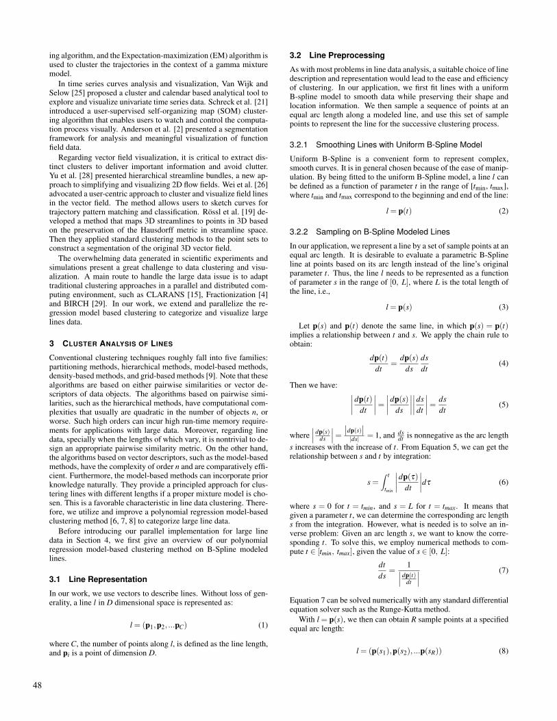
Aswith most problems in line data analysis, a suitable choice of linedescription and representation would lead to the ease and efficiencyof clustering. In our application, we first fit lines with a uniformB-spline model to smooth data while preserving their shape andlocation information. We then sample a sequence of points at anequal arc length along a modeled line, and use this set of samplepoints to represent the line for the successive clustering process.
3.2.1 Smoothing Lines with Uniform B-Spline Model
Uniform B-Spline is a convenient form to represent complex,smooth curves. It is in general chosen because of the ease of manip-ulation. By being fitted to the uniform B-Spline model, a line l canbe defined as a function of parameter t in the range of [tmin, tmax],where tmin and tmax correspond to the beginning and end of the line:
l= p(t) (2)
3.2.2 Sampling on B-Spline Modeled Lines
In our application, we represent a line by a set of sample points at anequal arc length. It is desirable to evaluate a parametric B-Splineline at points based on its arc length instead of the line’s originalparameter t. Thus, the line l needs to be represented as a functionof parameter s in the range of [0, L], where L is the total length ofthe line, i.e.,
l= p(s) (3)
Let p(s) and p(t) denote the same line, in which p(s) = p(t)implies a relationship between t and s. We apply the chain rule toobtain:
dp(t)
dt=
dp(s)
ds
ds
dt(4)
Then we have:∣
∣
∣
∣
dp(t)
dt
∣
∣
∣
∣
=
∣
∣
∣
∣
dp(s)
ds
∣
∣
∣
∣
∣
∣
∣
∣
ds
dt
∣
∣
∣
∣
=ds
dt(5)
where
∣
∣
∣
dp(s)ds
∣
∣
∣=
∣
∣dp(s)∣
∣
|ds| = 1, and dsdt is nonnegative as the arc length
s increases with the increase of t. From Equation 5, we can get therelationship between s and t by integration:
s=∫ t
tmin
∣
∣
∣
∣
dp(τ)
dt
∣
∣
∣
∣
dτ (6)
where s = 0 for t = tmin, and s = L for t = tmax. It means thatgiven a parameter t, we can determine the corresponding arc lengths from the integration. However, what is needed is to solve an in-verse problem: Given an arc length s, we want to know the corre-sponding t. To solve this, we employ numerical methods to com-pute t ∈ [tmin, tmax], given the value of s ∈ [0, L]:
dt
ds=
1∣
∣
∣
dp(t)dt
∣
∣
∣
(7)
Equation 7 can be solved numerically with any standard differentialequation solver such as the Runge-Kutta method.
With l= p(s), we then can obtain R sample points at a specifiedequal arc length:
l= (p(s1),p(s2), ...p(sR)) (8)
48

3.3 Regression Model-based Clustering
3.3.1 Linear Regression Models
Regression is a method for fitting a line through a set of points us-ing some goodness-of-fit criterion. One of the most common typesof regression is linear regression. Let x be an independent variable,and let p(x) denote an unknown function of x that we want to ap-proximate. Assume there are R observations, i.e., the values of p(x)measured at the specified values of xr are given as:
p(xr) = pr, r = 1, · · · ,R. (9)
Regarding each dimension of one line p(x), the idea behind lin-ear regression is to model p(x) by a linear combination of Q basisfunctions:
p(x)≈ β1ψ1(x)+ · · ·+βQψQ(x) (10)
In our case, we use polynomial basis functions, namely,
p(x)≈ β0+β1x+ · · ·+βQxQ (11)
If we consider a line l =(
p(x1), p(x2), . . . , p(xR))
, Equation 11can be written as,
l= Xβ + ε (12)
where l is a matrix of R×D, representing a line of length R in Ddimensional space. β is a Q×D dimensional matrix of regressioncoefficients, and ε is an R×D noise matrix. X is the usual R×QVandermonde regression matrix:
X=
x10 x1
1 x12 . . . x1
Q
x20 x2
1 x22 . . . x2
Q
......
......
...
xR0 xR
1 xR2 . . . xR
Q
(13)
3.3.2 Model-based Clustering
Model-based clustering can be regarded as the generalization of theK-means algorithm [10, 12]. In the context of model-based cluster-ing, the whole set of lines is assumed to be derived from a mixturemodel ofK components that correspond toK clusters. Each compo-nent model is associated with a probabilistic density function. Withregard to our case, each line is represented by a mixture model ofK component polynomial regression models with Gaussian errorterms, as shown in Equation 12. Let pk denote the probability atwhich a line is generated by the cluster k, and then the mixture den-sity for generating one line l is:
p(l|Θ) = ∑k
αkpk(l|θk) (14)
where αk denotes the probability of cluster k, which is nonnega-tive and all component probabilities (for k = 1 . . .K) sum to one.θk indicates the parameters of component model k. Each compo-nent θk contains regression coefficients βk and Gaussian covari-ance parameter δk. Thus, the mixture model is represented asΘ = {θ1, · · · , θK}.
pk(l|θk)means the probability of component model k generatingline l. In our work, the model component takes a form as Equation12. As a result, the regression model leads to a cluster-specificprobabilistic density function for l:
pk(l|θk) = N (l|Xβk, σk2I)
=R
∏r=1
N (pr|Xβk, σk2I) (15)
where N (�) is a D dimensional Gaussian probability density func-
tion; Xβk and σk2I are the mean vector and covariance matrix of
the kth Gaussian density function, respectively.As a flavor of K-means method, the objective function of model-
based clustering maximizes the likelihood, L (Θ|L), of generatingthe line data set L(L= {l1, l2, . . . , lN}), given the mixture model Θ.In practice, the likelihood can be represented by any function of Θthat is proportional to the probability p(L|Θ). In our application,the log of the likelihood of L is applied:
L (Θ|L) = log p(L|Θ) = ∑n
logK
∑k
αkpk(ln|θk) (16)
To this end, conducting model-based clustering is to estimate theparameters of theK component models given a set of lines, and thento assign each line to a cluster with the highest probability amongall K clusters. The Expectation-Maximization (EM) algorithm pro-vides an efficient framework for parameter estimation in the mix-ture model context [5], and we choose it for our model-based clus-tering. In the polynomial regression model-based clustering, theEM algorithm is executed as follows.
• E-Step: We assume that yn, associated with each ln, indicatesthe line membership in one of the K clusters. The posteriorp(yn|ln) is calculated to give the probability that the nth lineis generated by cluster yn. The probability of ln generated bycluster k takes the form [7]:
wnk = p(yn = k|ln)∝ αkpk(ln) = αkN (ln|Xβk, σk2I) (17)
• M-Step: The likelihood in Equation 16 is maximized withrespect to the parameters {βk, σk
2, αk}. The solutions [7] aregiven as:
βk =[
∑n
wnkX′nXn
]−1∑n
wnkX′nln (18)
σ2k =
1
∑nwnk∑n
wnk‖ln−Xnβk‖2 (19)
αk =1
N∑n
wnk (20)
After obtaining these mixture model parameters, we can use themto compute the probability value by Equation 15, and then refereach line to a cluster with the highest probability value.
4 PARALLEL IMPLEMENTATION
To process large line data, we implement our regression model-based clustering using a hybrid approach with MPI and CUDA byleveraging the power of CPUs and GPUs on multiple nodes in a het-erogeneous environment. To ensure the feasibility and scalability ofour approach, we consider the complete course of our clustering ap-proach, design the parallel implementation of each step and assignthem to the CPUs and/or GPUs based on their characteristics andassociated constraints.
First, for the line preprocessing step (Section 3.2), we couldtreat it as a one-time preprocessing step, save the resulted B-Splinemodeled lines, and repeatedly load them for later different cluster-ing runs to generate clusters with different inputs. However, giventhe sheer size of line data, it is generally desired to minimize stor-age overhead for particular analysis tasks, thus requiring us to per-form line preprocessing on-the-fly. We note that the operations ofsmoothing and sampling on different lines are independent of each
49

Algorithm 1 Parallel Regression Model-based Clustering
Input: N lines; M compute nodes.Output: K clusters.1: // Partitioning and distributing N lines to M nodes2: for each compute node in parallel do3: Performs the sorted balancing algorithm independently to
decide its own line assignment4: Performs MPI collective I/O to fetch its own line data5: end for6: // Preprocessing7: for each compute node in parallel do8: Transfers its lines from CPU to GPU9: Smooths its lines with uniform B-Spline model on GPU
10: Samples its lines to obtain their vector descriptors on GPU11: Copies the line vector descriptors from GPU to CPU12: end for13: // Initialization14: for each compute node in parallel do15: Randomly initializes the probability pik of each local line li
belonging to a cluster k, constrained by ∑Kk=1 pik = 1
16: end for17: All nodes calculate βk,σ
2k ,αk according to Equations 18, 19
and 20 using the psgels routine of SCALAPACK18: // Model-based clustering19: while true do20: // E-Step21: for each compute node in parallel do22: Calculates the probability pik of each local line li be-
longing to a cluster k by Equation 17, constrained by
∑Kk=1 pik = 1
23: end for24: // Likelihood calculation25: All nodes all gather the total likelihood L in Equation 1626: if the increment of L is less than a specified threshold or
the iteration number is greater than a specified limit then27: break28: end if29: // M-Step30: All nodes calculate βk,σ
2k ,αk according to Equations 18, 19
and 20 using the psgels routine of SCALAPACK31: end while32: // Generating final membership33: for each compute node in parallel do34: Puts each local line li to a cluster k where the line has the
highest probability pik35: end for
other, which allows us to carry out the preprocessing step efficientlyon the GPUs.
Second, for the clustering step (Section 3.3), researchers [11, 18]have been developing different implementations of the EM algo-rithm to estimate mixture Gaussian models in parallel. We extendthe parallel EM algorithm with respect to regression mixture mod-els. Different from Gaussian mixture models, regression mixturemodels describe a group of lines with a regression line and the as-sociated deviation. One key step is to obtain {βk, σk
2, αk} bysolving Equation 12 as a linear least square problem. Such a solv-ing step can be performed more efficiently on the CPU than on theGPU, because the solving step is bandwidth limited and the currentbandwidth between the CPU and the GPU is lower than that of theCPU’s bus [23]. Therefore, in our design, we choose the SCALA-PACK package with the optimized CPU BLAS to solve the linearleast square problem on large data using multiple CPUs.
Third, we need to design a data partitioning and distributionscheme to favor both the preprocessing step and the clustering step,
Algorithm 2 Sorted Balancing
Input: list of lengths and indexes of N lines; number of computenodesM.
Output: assigned line list Am, where m ∈ [1,M].1: For each node m, set its assigned line list Am← ∅, and set its
assigned accumulated line length Lm← 02: Sort the input line list in a decreasing order of their lengths3: for each line l in the sorted line list do4: Let d be the node whose Ld is minimal5: // Assign l to the node d6: Ad ← l’s index7: Ld ← Ld + l’s length8: end for
and minimize the overhead of data transformation and transfer be-tween different steps. The challenge comes from the disparity ofdata partition requirements between different operations to achievea balanced workload. For the operations of smoothing and sam-pling in the preprocessing step, and for the operation of E-Step,each atomic operand is an individual line, implying a partition ofthe lines with respect to their associated operation costs. For theoperation of M-Step, the operands are the matrix presentations ofall lines, and the corresponding solver provided by SCALAPACKrequires an even partition of the matrices. In our design, we usea sorted balancing algorithm to partition and distribute the lines toachieve a well-balanced workload for each step and minimize theinter-node communication cost for data exchanges.
Algorithm 1 lists the detailed procedure of our parallel regressionmodel-based clustering. We first partition and distribute the lines tomultiple compute nodes based a sorted balancing algorithm. Afterobtaining its line assignment, each node first smooths lines with theB-Spline model and then samples the lines to obtain their vectordescriptors. This step is performed on the GPUs by exploiting thehigh levels of concurrency enabled by CUDA. Next, the parallelmodel-based clustering algorithm is launched to collectively find anumber of clusters based on the line vector descriptors. Our linepartition and distribution scheme makes it possible to leverage thescalability of SCALAPACK and perform this step efficiently acrossthe CPUs. Thus, by considering the characteristics of different stepsand the interplay between them, we carefully distribute the work-loads of different steps among the different processing units andcan maximize the utilization of the heterogeneous computers.
4.1 Lines Partitioning and Distribution
We need partition and distribute the lines with different lengths tomultiple compute nodes and ensure the balanced workload of eachstep assigned to the nodes. First, in the preprocessing step and theE-Step, we note that each line is processed independently of eachother. Moreover, as we sample a line at an equal arc length, theworkload associated with a line is proportional to its length. Thus,the total length of lines assigned to each node should be approxi-mately equal.
Second, given the vector descriptors of lines, we construct thematrices l, X, β , and ε in Equation 12, where the row number ofl, X and ε is equal to the total sampling point number of all lines.To solve such a large system in the M-Step, we use the psgels rou-tine of SCALAPACK, which requires to evenly divide the matricesalong rows to produce a Cartesian distribution of each matrix 1. Wecan implicitly divide these large matrices by constructing the localmatrices from the local vector descriptors at each node. However,as the local total sampling point number at each node is not neces-
1Compared with the total number of sampling points, the dimension D
is relatively small (such as two or three) in our current study. Thus we did
not divide the matrices along columns.
50

# avg points # avg samples # compute nodescase data set # lines per line per line 1 2 3 4 5 6 7 8
1 (small case) solar plume 10,000 501 71 x x x x x x x x2 (small case) combustion 10,000 101 35 x x x x x x x x3 (medium case) combustion 100,000 101 35 x x x x x x x x4 (large case) combustion 1,000,000 101 35 x x x x x
Table 1: Setup of scalability study. Entries marked with “x” represent experiment runs.
sarily the same, the constructed local matrices can have the differ-ent numbers of rows. One possible solution is to exchange partialvector descriptors among the nodes to make all the local matriceshave a same or nearly same number of rows. But this method re-quires the message exchanges of partial vector descriptors possiblyamong all nodes at each iteration of the Model-based clustering. Onthe other hand, we note that if the total length of lines assigned toeach node is nearly equal, the differences of total length of the localvector descriptors among the nodes are marginal. It allows us toappend a minimal number of rows of zeros to the local matrices tomake them have the same number of rows. This method achievesthe same solving results without involving communication cost, andthe computational overhead due to the extra zeros is negligible inpractice.
To this end, we use a sorted balancing algorithm in our work todivide and assign the lines among the nodes. Algorithm 2 sketchesour sorted balancing algorithm. The only inputs to the algorithmare the list of lengths and indexes of all lines and the number ofcompute nodes. Each node executes the sorted balancing algorithmindependently to calculate the line assignment that makes the totalline length assigned to each node is nearly equal.
By the sorted balancing algorithm, each node can obtain the in-dex list of its assigned lines. For each node, the assigned linedata may not be contiguously stored in the original line data file.To minimal the I/O overhead for each node fetching its own linedata from the storage, we first use MPI Type create struct andMPI File set view to set a file view for each node with respect toits own list of assigned line indexes and the list of line offsets. Andthen all nodes use the MPI collective I/O routine MPI File read allto collaboratively fetch its own line data in parallel.
4.2 Line Preprocessing
On each compute node, the preprocessing stage takes advantage ofthe parallel capability of GPUs to smooth and sample the bunch oflines. The operations of smoothing and sampling performed on oneline is independent of other lines. This allows us to use the typi-cal CUDA program model to process each line using one CUDAthread. After fetching its own line data from the storage, each nodetransfers the line data from the main memory to the GPU memorygiven the line representation as described in Section 3.1. Then, a
kernel SMOOTH-SAMPLE is called on a grid of NB thread blocks,
where N is the number of lines assigned to one processor and Bis the thread number of each block. The appropriate value of Bdepends on the available GPU resources, such as on-chip sharedmemory and registers. Each thread in the SMOOTH-SAMPLE ker-nel first smooths a line using the uniform B-Spline Model, and thengenerates a set of sample points along the line at a specified equalarc length. Then, the set of sample points of each line are trans-ferred back from the GPU memory to the main memory, which areused as the vector descriptors for the successive clustering step.
4.3 Model-based Clustering
After preprocessing, each node obtains a vector descriptor for eachlocal line. During the initialization stage of the clustering, givena specific target cluster number K, each node first randomly as-signs a probability value pik of each local line li belonging to a
cluster k. Each node constructs its local matrices l, X, β , and εin Equation 12. A minimal number of rows of zeros are appendedto the end of the matrices to make them have the same number ofrows among all nodes. Then the linear least square solver psgelsof SCALAPACK is called to solve βk, σ2
k , and αk according toEquations 18, 19 and 20 with the initial guess of probability values.After the initialization stage, the clustering then carries out the it-erative EM algorithm, until the overall likelihood has converged atan optimal value or the iteration number is greater than a specifiedlimit. Finally, each node puts each local line li to a cluster k wherethe line has the highest probability value pik to generate the finalmembership.
4.3.1 E-Step
The E-Step is responsible for calculating the probability of assign-ing lines into each cluster, which can be executed independently foreach line. Although we could use CUDA to implement a kernel forthis step, such computing is bandwidth limited, and the data trans-ferring cost between the CPU and the GPU can exceed the com-putational saving obtained on the GPU. Therefore, we advocate asimple CPU implementation that lets each node iterate through alllocal lines and compute the probability densities of each line be-longing to each of the mixture components according to Equation17.
4.3.2 M-Step
The M-Step estimates the parameters of each component regressionmodel, βk, σ2
k and αk. We use a linear least square solver to esti-mate βk according to Equation 18. Since the whole line data set isdistributed across different nodes, we choose the linear least squaresolver psgels of SCALAPACK using multiple CPUs. Then we em-ploy the matrix multiplication routine psgemm of SCALAPACKto calculate σ2
k according to Equation 19. The size of αk is 1×K,where K is the number of clusters. αk is obtained to all proces-sors using the MPI Allreduce routine. Note that the local matricesof all nodes have been made to have the same number of rows byappending a minimal number of rows of zeros, and such append-ing only needs to be done once during the initialization stage. Inthis way, we can satisfy the data partition specifications posed bySCALAPACK and ensure the balanced workloads of the solvers onmultiple CPUs.
5 RESULTS AND DISCUSSION
We have experimented our parallel polynomial regression model-based clustering on a heterogeneous system containing 8 nodesconnected by the Gigabit Ethernet. Each node contains one Intelquad-core 3.00GHz CPU with 4GB of memory, and one NVIDIAGeForce GTX 285 GPU.
The line data sets from two large scientific simulations have beenused in our experimental study. The first data set contains 10,000streamlines extracted from the vector field of a solar plume sim-ulation provided by the scientists at the National Center for At-mospheric Research. The domain grid size of the vector field is504×504×2048 and the average streamline length is proportionalto the domain diagonal. The second data set contains the time se-ries curves correlating multiple variables, which are generated from
51

Case1
Case2
Case3
Case4
Smoothing Time Sampling Time E-Step Time M-Step Time
Figure 1: Speedups of scalability study. In each plot, the horizontal axis represents the number of nodes, and the vertical axis represents therunning time in second. The left to the right columns show the timing results of smoothing, sampling, E-Step, and M-Step, respectively, for Cases1 to 4. The timing results corresponding to each case are plotted on the rows.
large-scale combustion simulations conducted by Sandia NationalLaboratories. This data set contains 1,000,000 time series curvesand each curve correlates, over 808 time steps, two key parametersin the phase space: mixture fraction and temperature.
We used these two data sets to design and conduct four sets ofscalability experiments with respect to the different problem sizes.Table 1 shows the experimental setup. We used the 10,000 stream-lines of the solar plume data set in Case 1, and the 1,000,000 timeseries curves of the combustion data set in Case 4. The curves ofCases 2 and 3 were obtained by randomly sampling the curves ofCase 4. We tested any number of compute nodes from 1 to 8 inCases 1 to 3, and any number of compute nodes from 4 to 8 in Case4. Figure 1 shows the performance results. Each row represents theresults for a set of scalability experiments. Each column representsthe results of the same operation for the different problem sizes.
The first column of Figure 1 shows the performance of thesmoothing operation performed on the GPUs. In general, thesmoothing time decreases accordingly as we use more computenodes. However, we notice that the timing roughly remains aboutthe same beyond 4 nodes for Case 1, and beyond 2 nodes for Case 2.The main possible reason is that when the node count increases to acertain number, the workload associated with the lines assigned to
each GPU may not invoke sufficient number of threads to fully uti-lize the parallelism provided by CUDA, and the performance gainobtained by the GPU can be suppressed by the data transfer over-head between the CPU and the GPU [16]. Consequently, the paral-lel efficiency is only 51.3% (8 nodes vs. 1 node) for Case 1. Theline number used in Case 2 is same as Case 1, but the average pointnumber per line in Case 2 is much smaller so that the parallel effi-ciency is even worse for Case 2, which is only 26.7% (8 nodes vs. 1node). In Cases 3 and 4, when much large line sets are considered,we can better exploit the GPU parallelism and improve the scala-bility performance. The parallel efficiencies are 72.5% and 98.4%for Case 3 (8 nodes vs. 1 node) and Case 4 (8 nodes vs. 4 nodes),respectively.
The second column of Figure 1 shows the performance of thesampling operation performed on the GPUs. Similar to the smooth-ing operation, the speedup of the sampling operation improves ac-cordingly when we increase the number of lines to saturate theGPU. The parallel efficiencies of sampling are 45.9%, 32.0%,75.3%, and 98.4% for Cases 1 to 4, respectively. Moreover, the highparallelism provided by the GPU allows us to perform the comput-ing intensive processing task efficiently. For instance, in our exper-imental study, the time to smooth and sample 100,000 lines using
52

Case 1 smoothing time (0.53%) Case 1 sampling time (1.64%) Case 1 E-Step time (0.11%) Case 1 M-Step time (0.03%)
Case 4 smoothing time (3.46%) Case 4 sampling time (2.09%) Case 4 E-Step time (0.16%) Case 4 M-Step time (0.01%)
Figure 2: Workloads among 8 nodes for Cases 1 and 4. In each plot, the horizontal axis represents the node ID, and the vertical axis representsthe running time in second. The left to the right columns show the timing results of smoothing, sampling, E-Step, and M-Step, respectively. Thepercentage number associated with each plot is the difference ratio between the maximum and minimum times among the nodes.
one GPU is about two orders of magnitude less than the one usingone CPU core.
The third column of Figure 1 shows the performance of the E-Step operation performed on the CPUs. For this operation, eachnode independently calculates the probability value of each localline belonging to a cluster, and no communications are required.Thanks to our sorted balancing algorithm, the E-Step achieves al-most ideal speedup, and the parallel efficiencies of E-Step are 99%,98%, 99.5%, and 96.7% for Cases 1 to 4, respectively.
The fourth column of Figure 1 shows the performance of the M-Step operation performed on the CPUs. The parallel efficiencies ofM-Step are only 52.3% and 19.5% for Cases 1 and 2, respectively,which are less satisfactory. The main possible reason is that thepsgels and psgemm routines of SCALAPACK are used to estimatethe parameters of each regression model in parallel, and inter-nodecommunications are required in these routines. When the numberof lines is relatively small, such as in Case 1 or 2, the communica-tion overhead can dominate the overall time of operation and incurperformance degradation with more nodes. When we increase thenumber of lines, the computing time of solving local linear sys-tems tends to dominate the overall time. With our sorted balancingalgorithm, the solving workload can be well-balanced among thenodes, and the parallel efficiencies of M-Step are 77.7% and 99.5%for Cases 3 and 4, respectively.
Figure 2 shows the workload of each operation among 8 nodesfor Cases 1 and 4 with respect to the small and large problem sizes.We define the difference ratio, dr, of the workloads as:
dr = (max time−min time)/max time,
where max time (min time) is the maximum (minimum) timeamong all nodes for the same operation. The dr values for the oper-ations of Cases 1 and 4 are shown in Figure 2. For instance, in termsof the smoothing time, the dr values are 0.53% and 3.46% for Cases1 and 4, respectively. In terms of the M-Step time, the dr values are0.03% and 0.01% for Cases 1 and 4, respectively. We can observethat based on our sorted balancing algorithm, we can achieve wellbalanced workloads for all operations in both the preprocessing andclustering stages. We note that each stage is performed on a differ-ent type of processor, and has a different data representation and adifferent data access pattern.
Figure 3 shows the clustering result of the 10,000 streamlines ofthe solar plume data set in Case 1, where eight clusters are gener-ated. Figure 3 (a) shows the overview of all streamlines, and Fig-
ure 3 (b)-(i) show the individual clusters of the streamlines. Byusing our clustering method, the bundle of lines are partitioned to anumber of clusters which facilitate recognition and understanding.Effective visualization results are generated to depict the differentstreamline features, by observing which people can perceive thecomplex structures and correlations inherent in the turbulent vectorfield more clearly.
Figure 4 shows the clustering result of the 100,000 time seriescurves of the combustion data set in Case 3, where fourteen clus-ters are generated. Figure 4 (a) shows the overview of all curveswhere the visual clutter is occurred, making it difficult for a user toperceive structure information. Figure 4 (b)-(j) show the individ-ual cluster of the curves after applying our clustering method. Wecan see that after clustering the data set is well partitioned, and eachcluster consists of similar curves, which allows scientists to observethe correlations between two variables more easily. Especially, thepatterns shown in Figure 4 (j) are the outliers that do not matchthe profile curves from the hypothesis, and the scientists want tocapture and isolate them for further study. For a detailed applica-tion based on the model-based clustering method, please refer toour recent work on visual analysis of turbulent combustion particledata [27].
6 CONCLUSIONS AND FUTURE WORK
We have demonstrated how clustering for visualization of large linedata can be done efficiently with a combination of multiple GPUsand CPUs. The key aspects of our work include how we prepareand distribute the line data to facilitate the clustering calculationsand how we devise and implement the model-based clustering al-gorithm in CUDA and MPI. The scientists we have worked with areeager to integrate this new visualization capability into their routinescientific data analysis and discovery process. Presently, the bestscenario for using our design is with in-situ construction of linesfollowed by interactive visualization of the lines using a GPU clus-ter. Later on, as we move to the petascale and exascale computing,we will likely have to also conduct clustering in situ and compressthe line data as much as possible to reduce storage and transfercosts. Other future research opportunities include metric design forcategorizing other types of line data, line data packing and stream-ing, and visualization of higher dimensional line data.
53

(a) (b) (c)
(d) (e) (f)
(g) (h) (i)
Figure 3: This figure shows the clustering result of the streamlines generated from the solar plume velocity vector field. (a) shows the overviewof all 10,000 streamlines. (b)-(i) show the eight different groups of streamlines.
(a) (b) (c) (d) (e)
(f) (g) (h) (i) (j)
(h) (i) (j) (k) (j)
Figure 4: This figure shows the clustering result of the time series curves relating two variables, mixture fraction (the red axis) and temperature(the green axis), in the combustion simulation. (a) shows the overview of all 100,000 time series curves. (b)-(j) show the fourteen different groupsof time series curves.
54

ACKNOWLEDGEMENTS
This work has been sponsored in part by the U.S. Department ofEnergy through the SciDAC program with Agreement No. DE-FC02-06ER25777, and by the U.S. National Science Foundationthrough grants OCI-0749227, CCF-0811422, OCI-0749217, OCI-0950008, and OCI-0850566. Sandia National Laboratories is amultiprogram laboratory operated by Sandia Corporation, a Lock-heed Martin Company, for the U.S. Department of Energy undercontract DE-AC04-94-AL85000. The solar plume data set is pro-vided by John Clyne at the National Center for Atmospheric Re-search.
REFERENCES
[1] W. Aigner, S. Miksch, W. Muller, H. Schumann, and C. Tominski.
Visual methods for analyzing time-oriented data. IEEE Transactions
on Visualization and Computer Graphics, 14(1):47–60, 2008.
[2] J. C. Anderson, L. Gosink, M. A. Duchaineau, and K. Joy. Interactive
visualization of function fields by range-space segmentation. Com-
puter Graphics Forum, 28(3):727–734, 2009.
[3] A. Brun, H. Knutsson, H. J. Park, M. E. Shenton, and C.-F. Westin.
Clustering fiber tracts using normalized cuts. In Proceedings of In-
ternational Conference on Medical Image Computing and Computer-
Assisted Intervention, pages 368–375, 2004.
[4] D. R. Cutting, D. R. Karger, J. O. Pedersen, and J. W. Tukey. Scat-
ter/gather: a cluster-based approach to browsing large document col-
lections. In Proceedings of ACM SIGIR Conference on Research and
Development in Information Retrieval, pages 318–329, 1992.
[5] A. P. Dempster, N. M. Laird, and D. B. Rubin. Maximum likelihood
from incomplete data via the em algorithm. Journal of the Royal Sta-
tistical Society, Series B, 39(1):1–38, 1977.
[6] S. Gaffney and P. Smyth. Trajectory clustering with mixtures of
regression models. In Proceedings of ACM SIGKDD International
Conference on Knowledge Discovery and Data Mining, pages 63–72,
1999.
[7] S. Gaffney and P. Smyth. Joint probabilistic curve clustering and
alignment. In Advances in Neural Information Processing Systems,
pages 473–480, 2004.
[8] S. J. Gaffney, A. W. Robertson, P. Smyth, S. J. Camargo, and M. Ghil.
Probabilistic clustering of extratropical cyclones using regression
mixture models. Climate Dynamics, 29(4):423–440, 2007.
[9] J. Han. Data Mining: Concepts and Techniques. Morgan Kaufmann
Publishers Inc., San Francisco, CA, USA, 2005.
[10] J. A. Hartigan and M. A. Wong. A k-means clustering algorithm.
JSTOR: Applied Statistics, 28(1):100–108, 1979.
[11] N. P. Kumar, S. Satoor, and I. Buck. Fast parallel expectation max-
imization for gaussian mixture models on GPUs using CUDA. In
Proceedings of IEEE International Conference on High Performance
Computing and Communications, pages 103–109, 2009.
[12] J. B. MacQueen. Some methods for classification and analysis of
multivariate observations. In Proceedings of Berkeley Symposium on
Mathematical Statistics and Probability, pages 281–297, 1967.
[13] M. Maddah, W. E. L. Grimson, S. K. Warfield, and W. M. Wells. A
unified framework for clustering and quantitative analysis of white
matter fiber tracts. Medical Image Analysis, 12(2):191–202, 2008.
[14] B. Moberts, A. Vilanova, and J. J. van Wijk. Evaluation of fiber clus-
tering methods for diffusion tensor imaging. In Proceedings of IEEE
Visualization Conference, pages 65–72, 2005.
[15] R. T. Ng and J. Han. Clarans: A method for clustering objects for
spatial data mining. IEEE Transactions on Knowledge and Data En-
gineering, 14:1003–1016, 2002.
[16] NVIDIA. CUDA C Best Practices Guide (version 4.0), May 2011.
[17] L. O’Donnell and C.-F. Westin. White matter tract clustering and cor-
respondence in populations. In Proceedings of International Confer-
ence on Medical Image Computing and Computer-Assisted Interven-
tion, pages 140–147, 2005.
[18] A. D. Pangborn. Scalable data clustering using GPUs. Master’s thesis,
Rochester Institute of Technology, 2010.
[19] C. Rossl and H. Theisel. Streamline embedding for 3D vector field ex-
ploration. IEEE Transactions on Visualization and Computer Graph-
ics, 99(PrePrints), 2011.
[20] T. Salzbrunn, H. Janicke, T. Wischgoll, and G. Scheuermann. The
state of the art in flow visualization: Partition-based techniques. In
SimVis, pages 75–92, 2008.
[21] T. Schreck, J. Bernard, T. Von Landesberger, and J. Kohlhammer. Vi-
sual cluster analysis of trajectory data with interactive kohonen maps.
Information Visualization, 8(1):14–29, 2009.
[22] J. S. Shimony, A. Z. Snyder, N. Lori, and T. E. Conturo. Automated
fuzzy clustering of neuronal pathways in diffusion tensor tracking.
In Proceedings of International Society for Magnetic Resonance in
Medicine, pages 453–456, 2003.
[23] S. Tomov, R. Nath, P. Du, and J. Dongarra. MAGMA Users Guide
(version 0.2), November 2009.
[24] A. Tsai, C.-F. Westin, A. O. Hero, and A. S. Willsky. Fiber tract
clustering on manifolds with dual rooted-graphs. In Proceedings of
IEEE Conference on Computer Vision and Pattern Recognition, pages
1–6, 2007.
[25] J. J. van Wijk and E. R. van Selow. Cluster and calendar based visu-
alization of time series data. In Proceedings of IEEE Symposium on
Information Visualization, pages 4–9, 1999.
[26] J. Wei, C. Wang, H. Yu, and K.-L. Ma. A sketch-based interface for
classifying and visualizing vector fields. In Proceedings of IEEE Pa-
cific Visualization Symposium, pages 129–136, 2010.
[27] J. Wei, H. Yu, R. W. Grout, J. H. Chen, and K.-L. Ma. Dual space
analysis of turbulent combustion particle data. In Proceedings of IEEE
Pacific Visualization Symposium, pages 91–98, 2011.
[28] H. Yu, C. Wang, C.-K. Shene, and J. H. Chen. Hierarchical streamline
bundles for visualizing 2D flow fields. In IEEE VisWeek 2010 Posters,
2010.
[29] T. Zhang, R. Ramakrishnan, and M. Livny. Birch: an efficient data
clustering method for very large databases. In Proceedings of ACM
SIGMOD international conference on Management of data, pages
103–114, 1996.
55