Embed Size (px)
Citation preview
1
Parallel Computing Introduction
Alessio Turchi
Slides thanks to:Tim Mattson (Intel)
Sverre Jarp (CERN)Vincenzo Innocente (CERN)
Outline
• High Performance computing: A hardware system view
• Parallel Computing: Basic Concepts
• The Fundamental patterns of parallel Computing
5
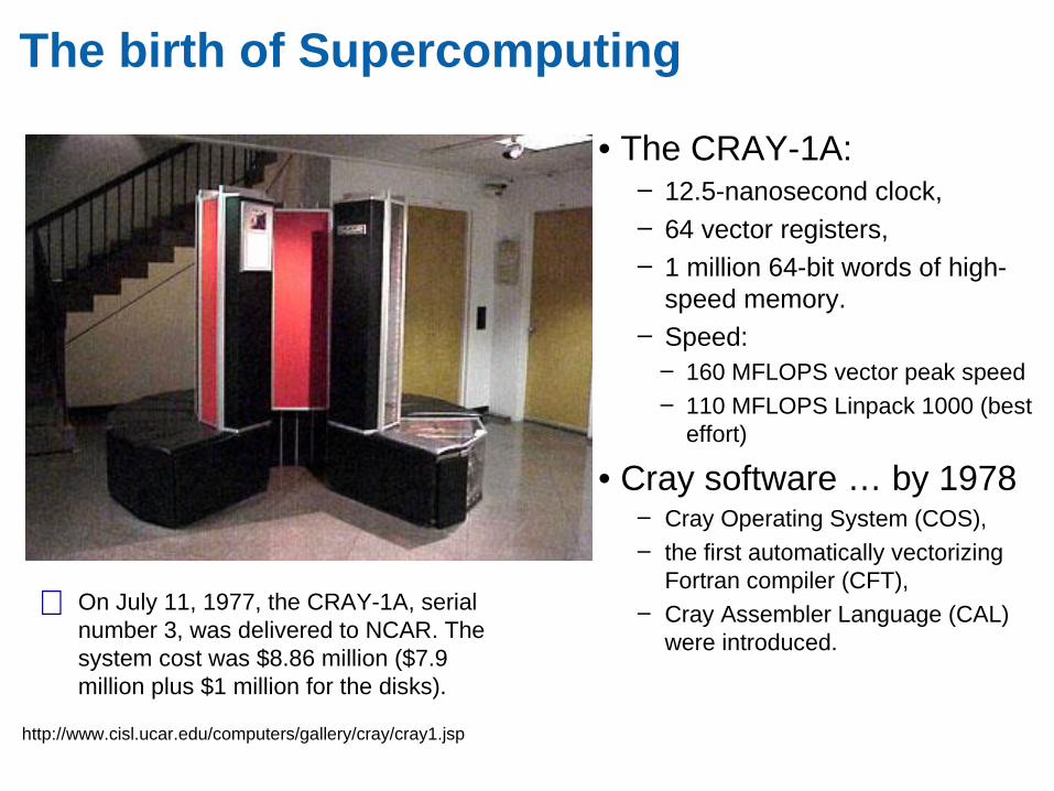
The birth of Supercomputing
• The CRAY-1A:– 12.5-nanosecond clock, – 64 vector registers,– 1 million 64-bit words of high-
speed memory. – Speed:
– 160 MFLOPS vector peak speed– 110 MFLOPS Linpack 1000 (best
effort)
• Cray software … by 1978 – Cray Operating System (COS), – the first automatically vectorizing
Fortran compiler (CFT),– Cray Assembler Language (CAL)
were introduced.
On July 11, 1977, the CRAY-1A, serial number 3, was delivered to NCAR. The system cost was $8.86 million ($7.9 million plus $1 million for the disks).
http://www.cisl.ucar.edu/computers/gallery/cray/cray1.jsp
0
10
20
30
40
50
60
Vector
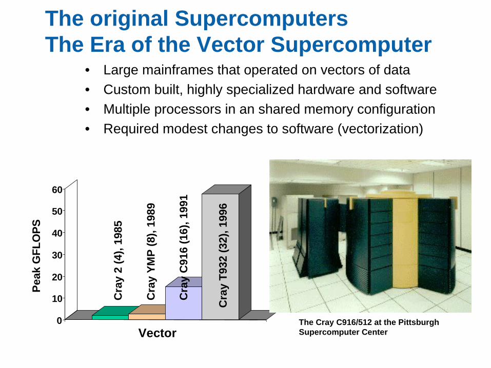
The original SupercomputersThe Era of the Vector Supercomputer
• Large mainframes that operated on vectors of data
• Custom built, highly specialized hardware and software
• Multiple processors in an shared memory configuration
• Required modest changes to software (vectorization)
The Cray C916/512 at the Pittsburgh Supercomputer Center
Cra
y 2
(4),
198
5
Cra
y Y
MP
(8)
, 198
9
Cra
y T
932
(32)
, 199
6
Pea
k G
FL
OP
S
Cra
y C
916
(16)
, 199
1
Vector
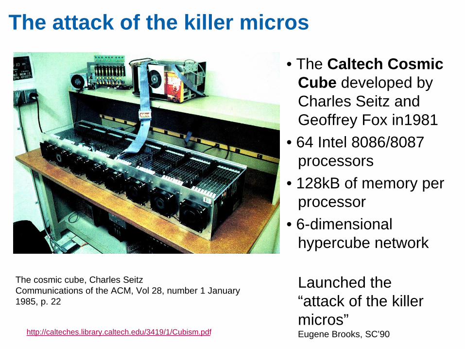
The attack of the killer micros
• The Caltech Cosmic Cube developed by Charles Seitz and Geoffrey Fox in1981
• 64 Intel 8086/8087 processors
• 128kB of memory per processor
• 6-dimensional hypercube network
http://calteches.library.caltech.edu/3419/1/Cubism.pdf
The cosmic cube, Charles SeitzCommunications of the ACM, Vol 28, number 1 January 1985, p. 22
Launched the “attack of the killer micros” Eugene Brooks, SC’90
0
204060
80100120
140160180200
Vector MPP
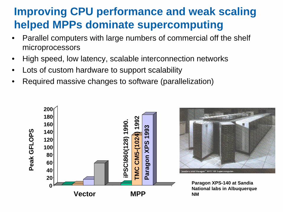
Improving CPU performance and weak scaling helped MPPs dominate supercomputing• Parallel computers with large numbers of commercial off the shelf
microprocessors
• High speed, low latency, scalable interconnection networks
• Lots of custom hardware to support scalability
• Required massive changes to software (parallelization)
Paragon XPS-140 at Sandia National labs in Albuquerque NM
Pea
k G
FL
OP
S
iPS
C\8
60(1
28)
1990
.
Par
ago
n X
PS
199
3
TM
C C
M5-
(102
4) 1
992
Vector MPP
10
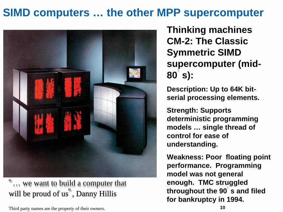
SIMD computers … the other MPP supercomputer
Thinking machines CM-2: The Classic Symmetric SIMD supercomputer (mid-80’ s):
Description: Up to 64K bit-serial processing elements.
Strength: Supports deterministic programming models … single thread of control for ease of understanding.
Weakness: Poor floating point performance. Programming model was not general enough. TMC struggled throughout the 90’ s and filed for bankruptcy in 1994.
Third party names are the property of their owners.
“ … we want to build a computer that will be proud of us” , Danny Hillis
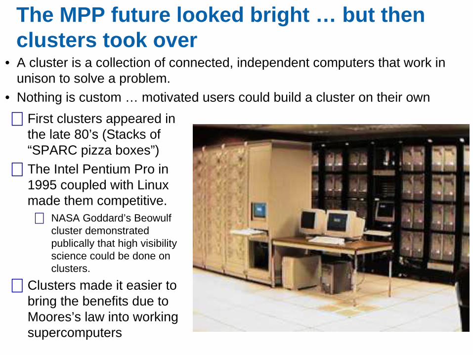
The MPP future looked bright … but then clusters took over
• A cluster is a collection of connected, independent computers that work in unison to solve a problem.
• Nothing is custom … motivated users could build a cluster on their own
First clusters appeared in the late 80’s (Stacks of “SPARC pizza boxes”)
The Intel Pentium Pro in 1995 coupled with Linux made them competitive.
NASA Goddard’s Beowulf cluster demonstrated publically that high visibility science could be done on clusters.
Clusters made it easier to bring the benefits due to Moores’s law into working supercomputers
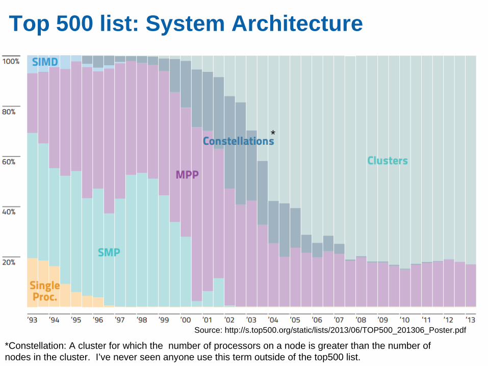
Top 500 list: System Architecture
*Constellation: A cluster for which the number of processors on a node is greater than the number of nodes in the cluster. I’ve never seen anyone use this term outside of the top500 list.
*
Source: http://s.top500.org/static/lists/2013/06/TOP500_201306_Poster.pdf
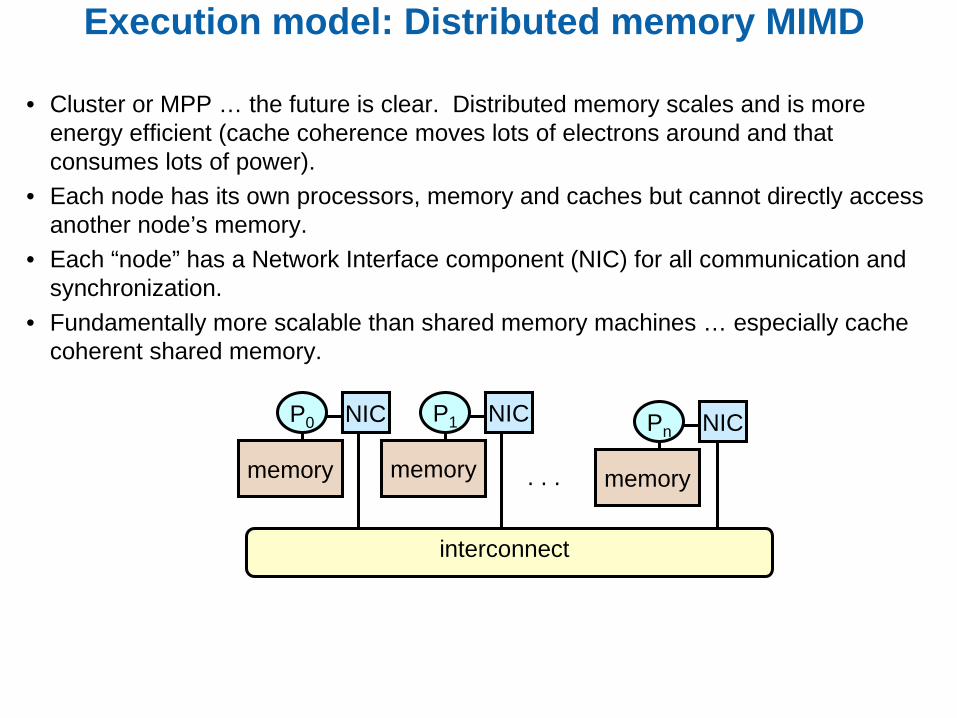
Execution model: Distributed memory MIMD
• Cluster or MPP … the future is clear. Distributed memory scales and is more energy efficient (cache coherence moves lots of electrons around and that consumes lots of power).
• Each node has its own processors, memory and caches but cannot directly access another node’s memory.
• Each “node” has a Network Interface component (NIC) for all communication and synchronization.
• Fundamentally more scalable than shared memory machines … especially cache coherent shared memory.
interconnect
P0
memory
NIC
. . .
P1
memory
NIC Pn
memory
NIC
Computer Architecture and Performance Tuning
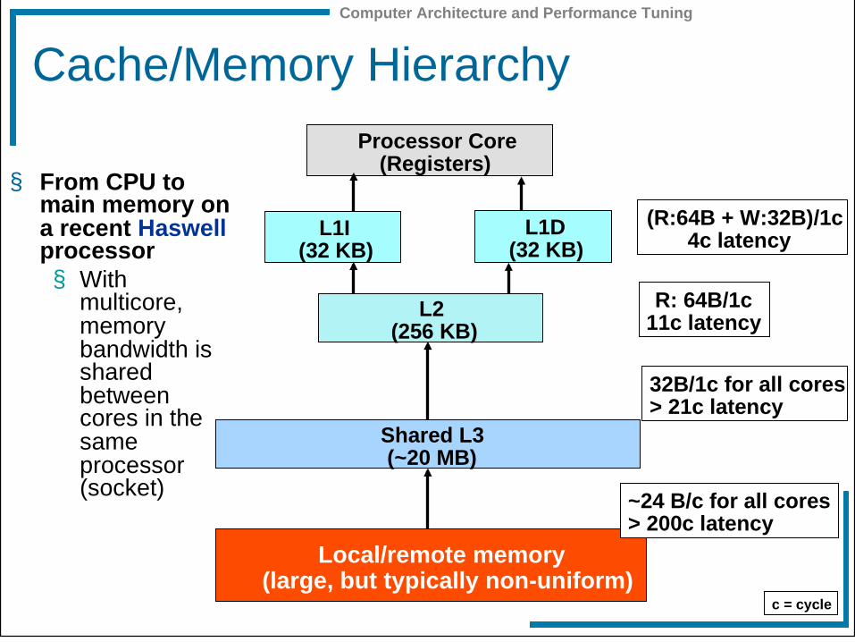
Cache/Memory Hierarchy
§ From CPU to main memory on a recent Haswell processor § With
multicore, memory bandwidth is shared between cores in the same processor (socket)
c = cycle
Processor Core (Registers)
Local/remote memory (large, but typically non-uniform)
R: 64B/1c 11c latency
~24 B/c for all cores > 200c latency
(R:64B + W:32B)/1c 4c latency
Shared L3 (~20 MB)
32B/1c for all cores > 21c latency
L2 (256 KB)
L1D (32 KB)
L1I (32 KB)
Computer Architecture and Performance Tuning
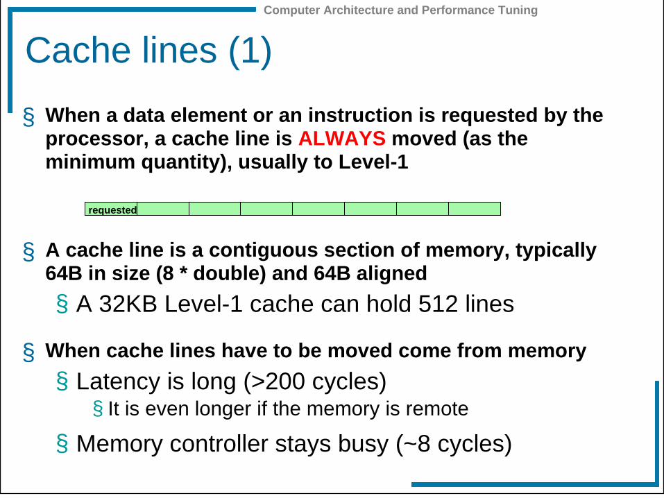
Cache lines (1)
§ When a data element or an instruction is requested by the processor, a cache line is ALWAYS moved (as the minimum quantity), usually to Level-1
§ A cache line is a contiguous section of memory, typically 64B in size (8 * double) and 64B aligned
§ A 32KB Level-1 cache can hold 512 lines
§ When cache lines have to be moved come from memory
§ Latency is long (>200 cycles) § It is even longer if the memory is remote
§ Memory controller stays busy (~8 cycles)
requested
Computer Architecture and Performance Tuning
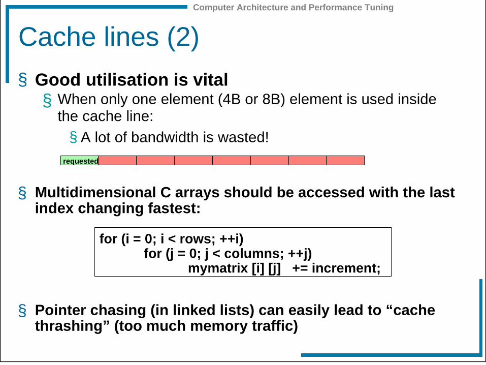
Cache lines (2)
§ Good utilisation is vital § When only one element (4B or 8B) element is used inside
the cache line:
§ A lot of bandwidth is wasted!
§ Multidimensional C arrays should be accessed with the last index changing fastest:
§ Pointer chasing (in linked lists) can easily lead to “cache thrashing” (too much memory traffic)
requested
for (i = 0; i < rows; ++i) for (j = 0; j < columns; ++j) mymatrix [i] [j] += increment;
Computer Architecture and Performance Tuning
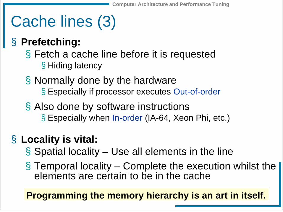
Cache lines (3) § Prefetching:
§ Fetch a cache line before it is requested § Hiding latency
§ Normally done by the hardware § Especially if processor executes Out-of-order
§ Also done by software instructions § Especially when In-order (IA-64, Xeon Phi, etc.)
§ Locality is vital: § Spatial locality – Use all elements in the line
§ Temporal locality – Complete the execution whilst the elements are certain to be in the cache
Programming the memory hierarchy is an art in itself.
Computer Architecture and Performance Tuning
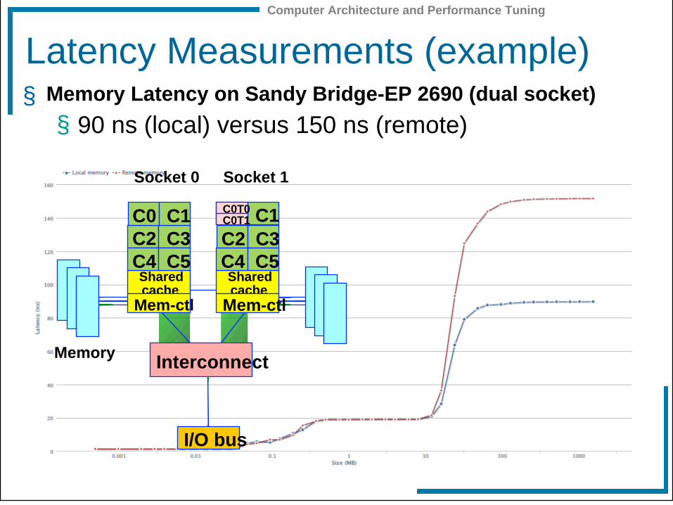
Latency Measurements (example) § Memory Latency on Sandy Bridge-EP 2690 (dual socket)
§ 90 ns (local) versus 150 ns (remote)
Interconnect
I/O bus
Shared cache
C2 C3 C4 C5
Mem-ctl
Shared cache
C0 C1
C4 C5
Mem-ctl
Memory
Socket 0 Socket 1
C0T0 C0T1 C0 C1 C2 C3
Computer Architecture and Performance Tuning
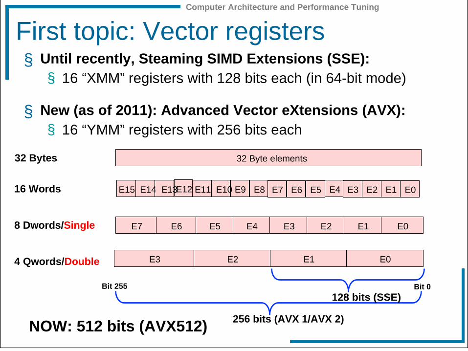
First topic: Vector registers § Until recently, Steaming SIMD Extensions (SSE):
§ 16 “XMM” registers with 128 bits each (in 64-bit mode)
§ New (as of 2011): Advanced Vector eXtensions (AVX): § 16 “YMM” registers with 256 bits each
E3 E2 E1 E0
E7 E6 E5 E4 E3 E2 E1 E0
Bit 0 Bit 255
E15 E14 E13 E12 E11 E10 E9 E8 E7 E6 E5 E4 E3 E2 E1 E0 16 Words
8 Dwords/Single
4 Qwords/Double
256 bits (AVX 1/AVX 2)
128 bits (SSE)
32 Byte elements 32 Bytes
NOW: 512 bits (AVX512)
Computer Architecture and Performance Tuning
Computer Architecture and Performance Tuning
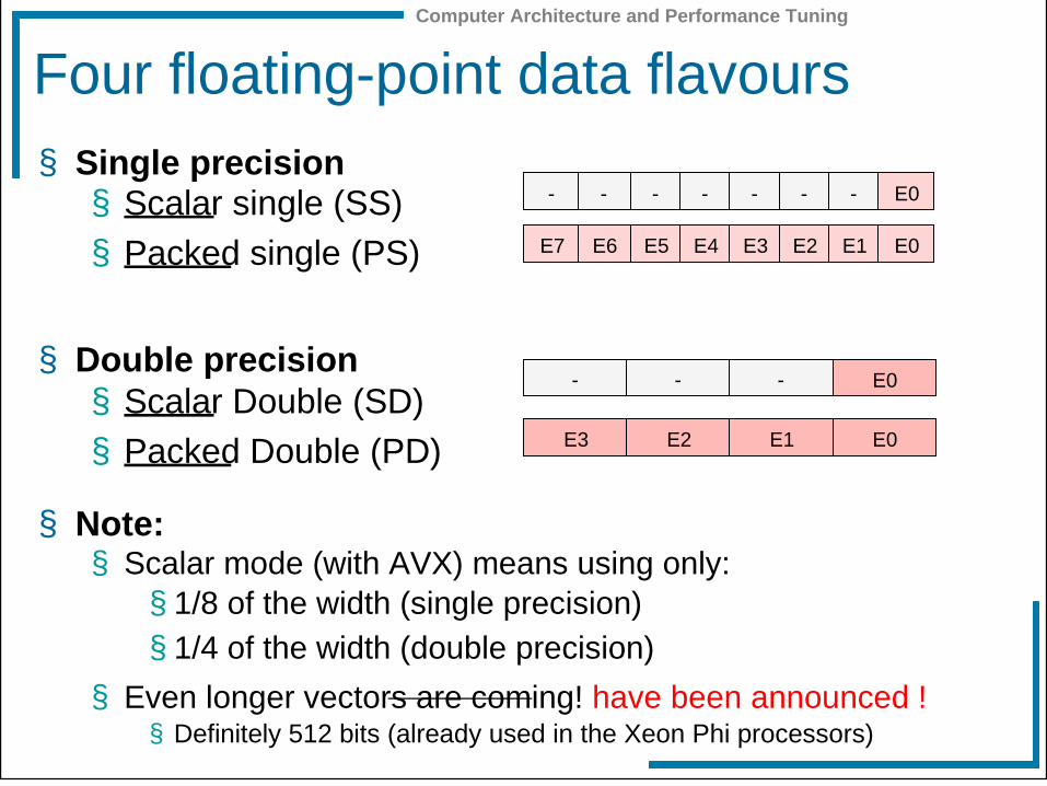
Four floating-point data flavours § Single precision
§ Scalar single (SS)
§ Packed single (PS)
§ Double precision § Scalar Double (SD)
§ Packed Double (PD)
§ Note: § Scalar mode (with AVX) means using only:
§ 1/8 of the width (single precision) § 1/4 of the width (double precision)
§ Even longer vectors are coming! have been announced ! § Definitely 512 bits (already used in the Xeon Phi processors)
E3 E2 E1 E0
- - - E0
E7 E6 E5 E4 E3 E2 E1 E0
- - - - - - - E0
Computer Architecture and Performance Tuning
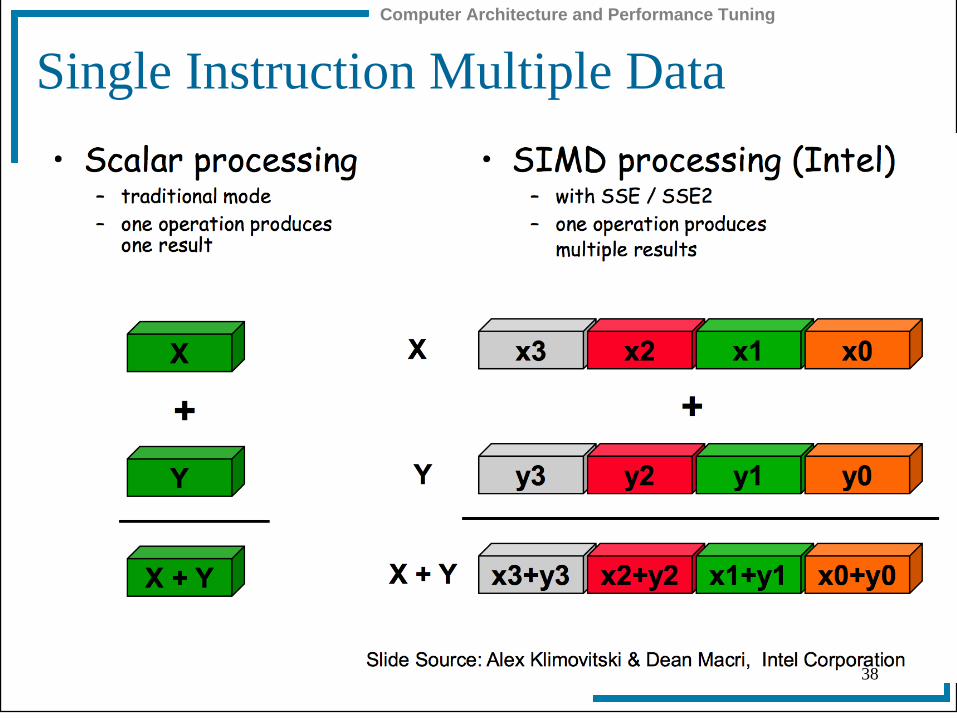
Single Instruction Multiple Data
22 October 2012 Vincenzo Innocente 38
Computer Architecture and Performance Tuning
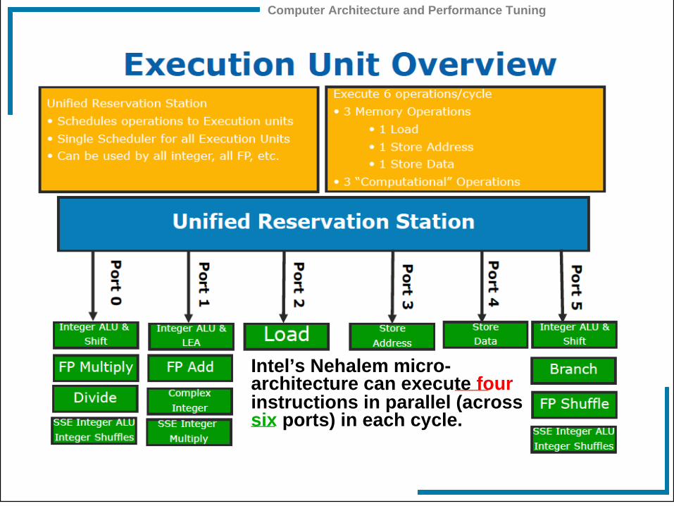
Intel’s Nehalem micro-architecture can execute four instructions in parallel (across six ports) in each cycle.
Computer Architecture and Performance Tuning
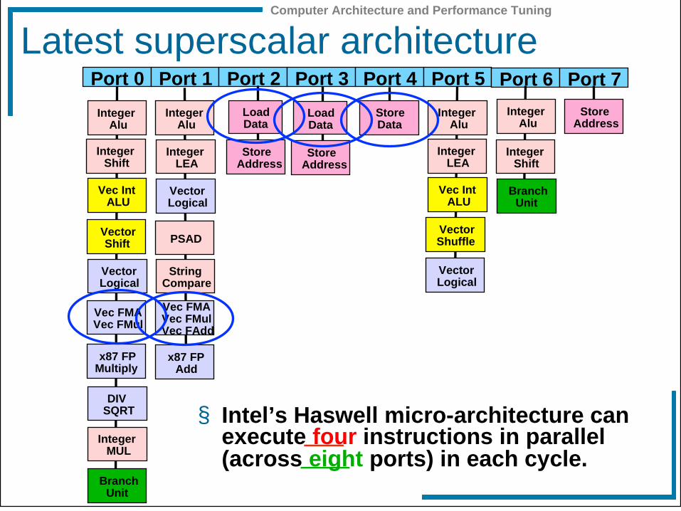
Latest superscalar architecture
§ Intel’s Haswell micro-architecture can execute four instructions in parallel (across eight ports) in each cycle.
Port 0 Port 1 Port 2 Port 3 Port 4 Port 5
Integer Alu
Vec Int ALU
x87 FP Multiply
Vec FMA Vec FMul
Vector Logical
Vector Shift
Integer Alu
Integer Alu
Vec Int ALU
Vector Logical
Vector Shuffle
Load Data
Store Data
Branch Unit
DIV SQRT
x87 FP Add
Vec FMA Vec FMul Vec FAdd
Integer Shift
Integer MUL
Integer LEA
PSAD
String Compare
Integer LEA
Port 6 Port 7
Store Address
Load Data
Store Address
Integer Alu
Store Address
Integer Shift
Branch Unit
Vector Logical
Computer Architecture and Performance Tuning
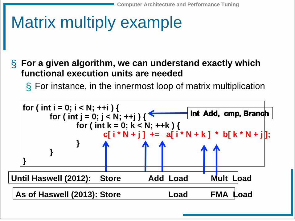
Matrix multiply example
§ For a given algorithm, we can understand exactly which functional execution units are needed
§ For instance, in the innermost loop of matrix multiplication
for ( int i = 0; i < N; ++i ) { for ( int j = 0; j < N; ++j ) { for ( int k = 0; k < N; ++k ) { c[ i * N + j ] += a[ i * N + k ] * b[ k * N + j ]; } }
}
Until Haswell (2012): Store Add Load Mult Load
As of Haswell (2013): Store Load FMA Load
Computer Architecture and Performance Tuning
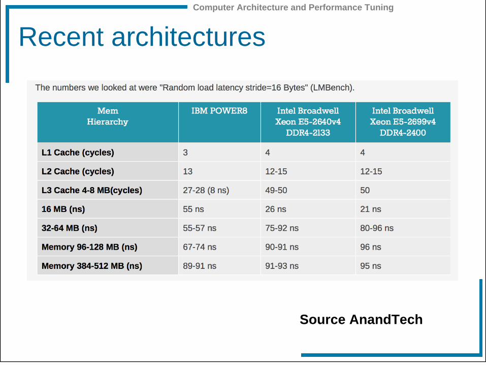
Recent architectures
Source AnandTech
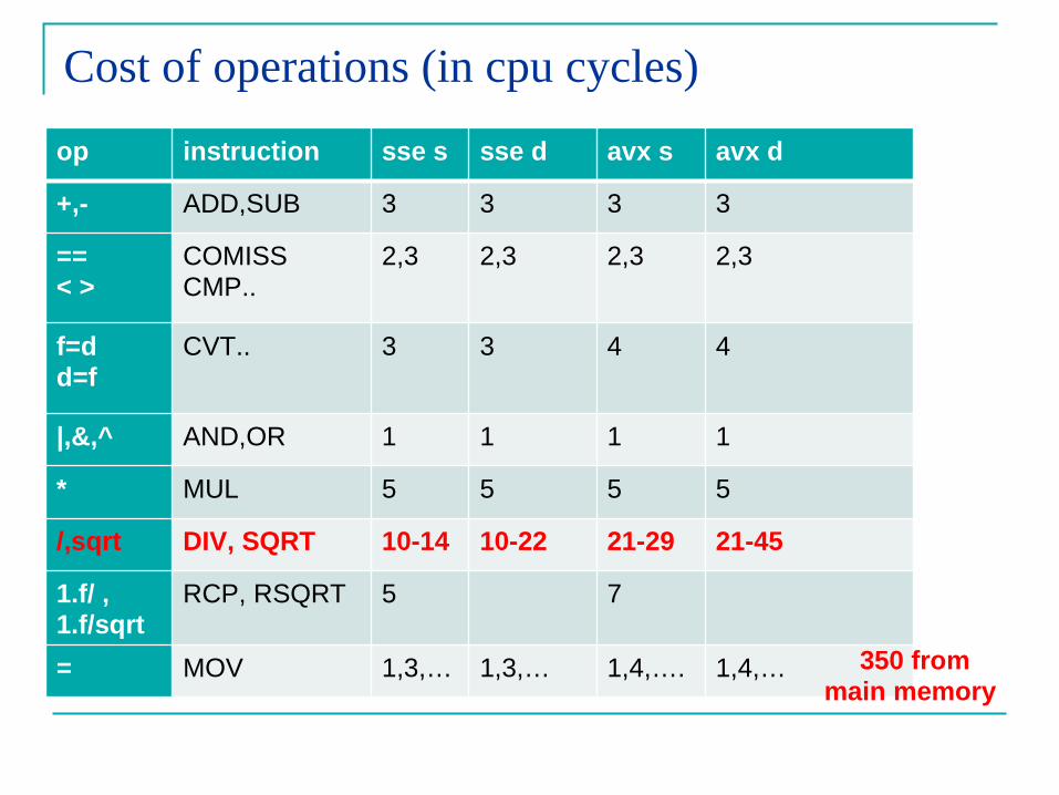
Cost of operations (in cpu cycles)
op instruction sse s sse d avx s avx d
+,- ADD,SUB 3 3 3 3
== < >
COMISS CMP..
2,3 2,3 2,3 2,3
f=d d=f
CVT.. 3 3 4 4
|,&,^ AND,OR 1 1 1 1
* MUL 5 5 5 5
/,sqrt DIV, SQRT 10-14 10-22 21-29 21-45
1.f/ , 1.f/sqrt
RCP, RSQRT 5 7
= MOV 1,3,… 1,3,… 1,4,…. 1,4,… 350 from main memory
Outline
• High Performance computing: A hardware system view
• Parallel Computing: Basic Concepts
• The Fundamental patterns of parallel Computing
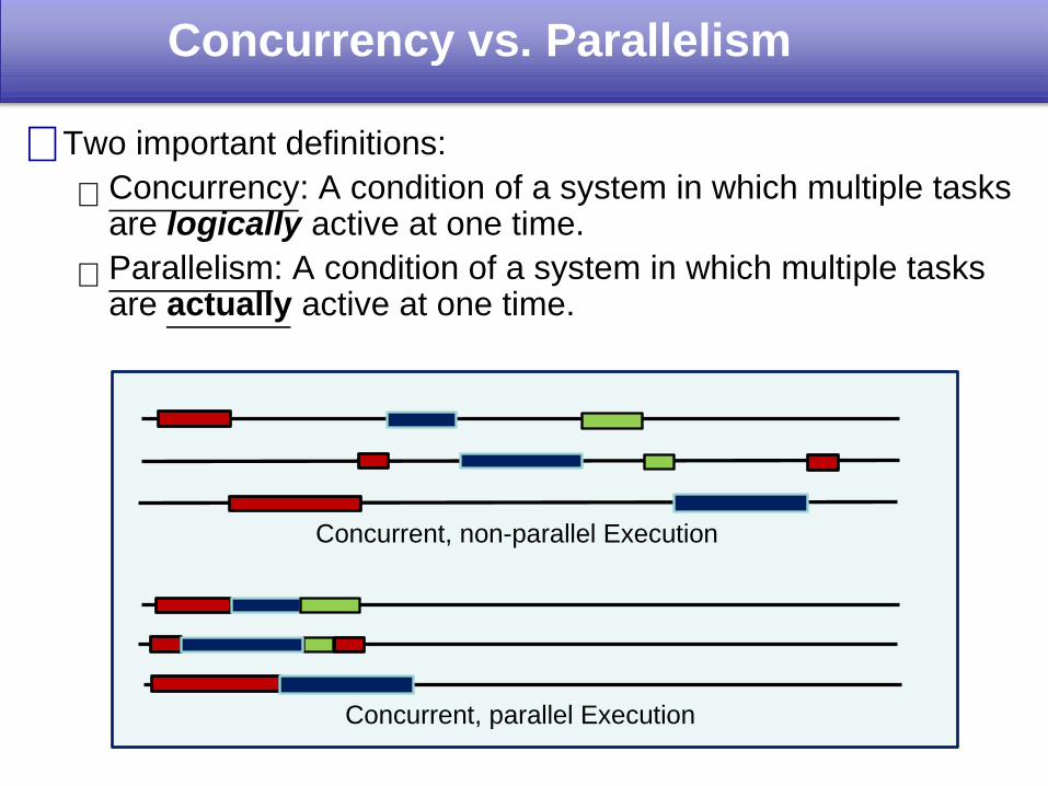
Concurrency vs. Parallelism
Two important definitions:
Concurrency: A condition of a system in which multiple tasks are logically active at one time.
Parallelism: A condition of a system in which multiple tasks are actually active at one time.
Concurrent, parallel Execution
Concurrent, non-parallel Execution
34
ImagesThe Internet
ImageServer
WebServer
Client
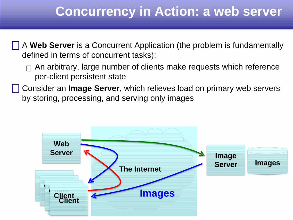
Concurrency in Action: a web server
Images
A Web Server is a Concurrent Application (the problem is fundamentally defined in terms of concurrent tasks):
An arbitrary, large number of clients make requests which reference per-client persistent state
Consider an Image Server, which relieves load on primary web servers by storing, processing, and serving only images
ClientClient
ClientClient
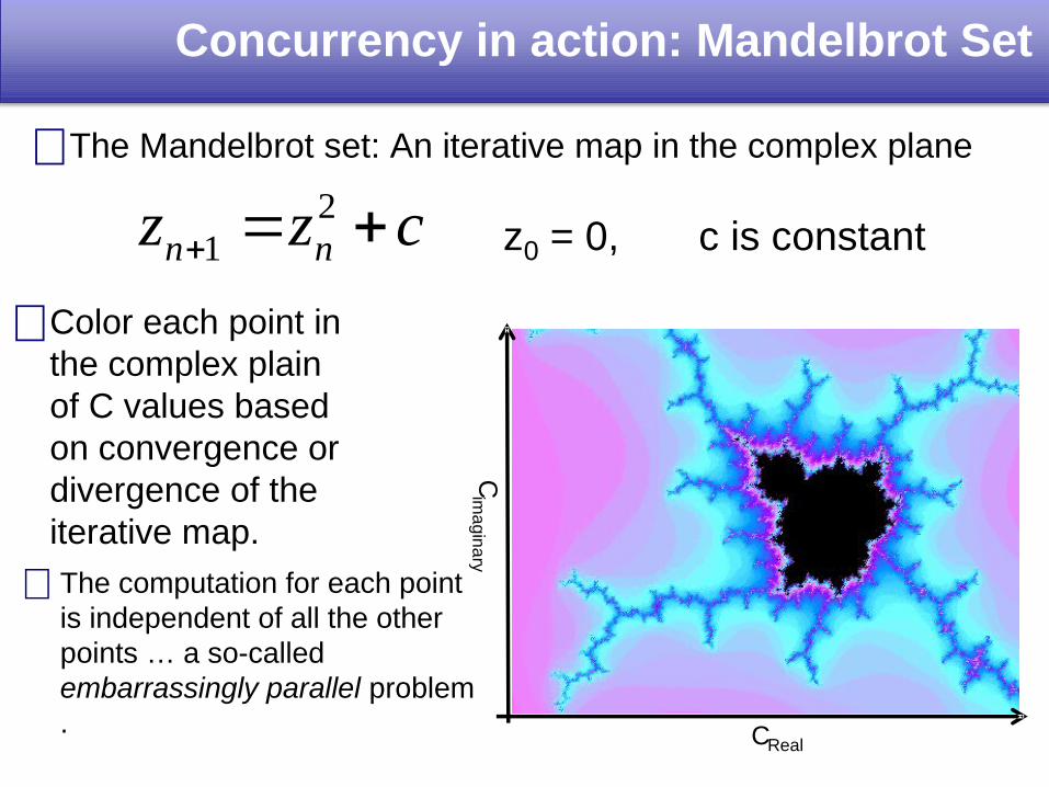
Concurrency in action: Mandelbrot Set
The Mandelbrot set: An iterative map in the complex plane
czz nn
21 z0 = 0, c is constant
Color each point in the complex plain of C values based on convergence or divergence of the iterative map.
CReal
Cim
ag
ina
ry
The computation for each point is independent of all the other points … a so-called embarrassingly parallel problem .
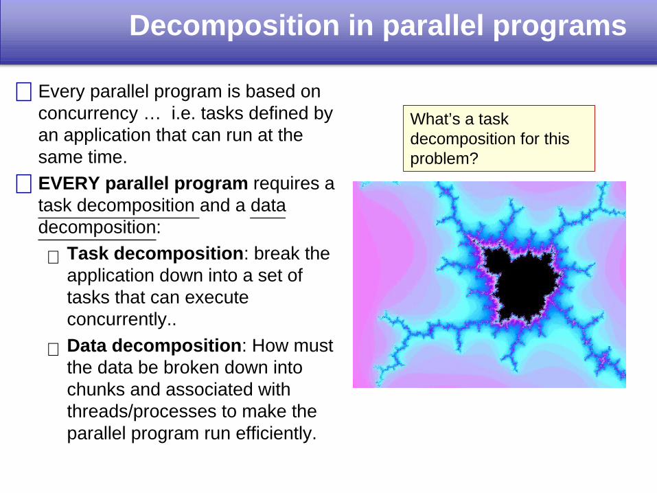
Decomposition in parallel programs
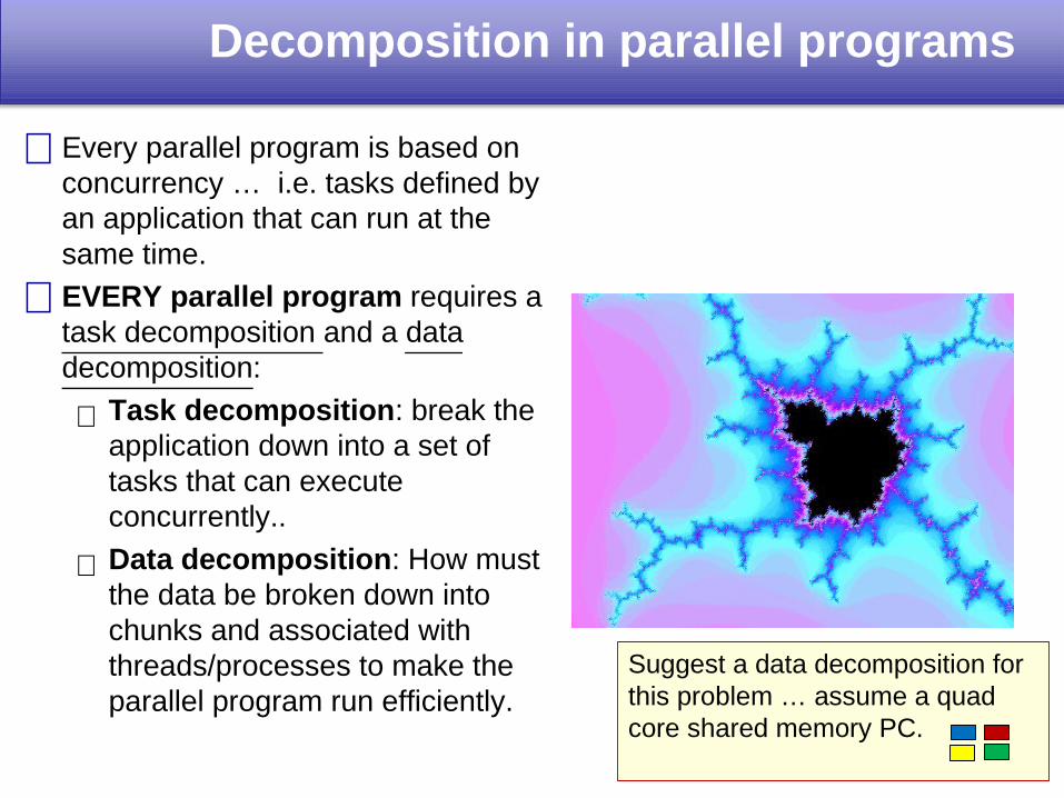
Every parallel program is based on concurrency … i.e. tasks defined by an application that can run at the same time.
EVERY parallel program requires a task decomposition and a data decomposition:
Task decomposition: break the application down into a set of tasks that can execute concurrently..
Data decomposition: How must the data be broken down into chunks and associated with threads/processes to make the parallel program run efficiently.
What’s a task decomposition for this problem?
51
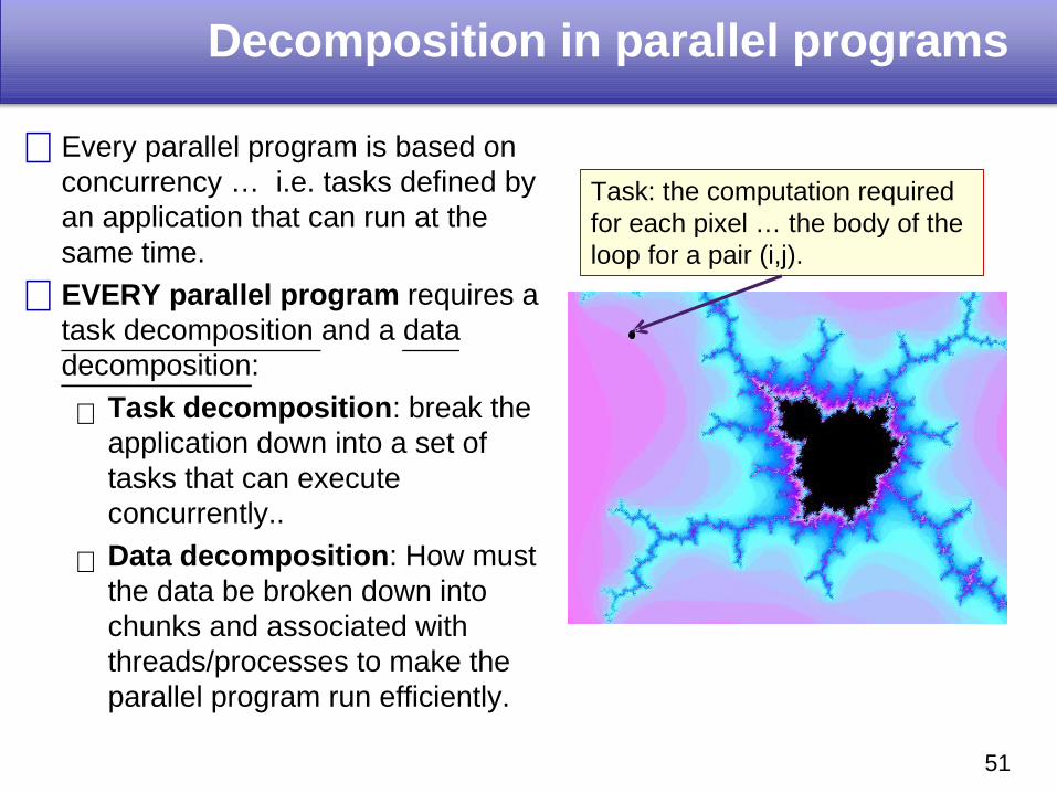
Decomposition in parallel programs
Every parallel program is based on concurrency … i.e. tasks defined by an application that can run at the same time.
EVERY parallel program requires a task decomposition and a data decomposition:
Task: the computation required for each pixel … the body of the loop for a pair (i,j).
Task decomposition: break the application down into a set of tasks that can execute concurrently..
Data decomposition: How must the data be broken down into chunks and associated with threads/processes to make the parallel program run efficiently.
52
Decomposition in parallel programs
Every parallel program is based on concurrency … i.e. tasks defined by an application that can run at the same time.
EVERY parallel program requires a task decomposition and a data decomposition:
Suggest a data decomposition for this problem … assume a quad core shared memory PC.
Task decomposition: break the application down into a set of tasks that can execute concurrently..
Data decomposition: How must the data be broken down into chunks and associated with threads/processes to make the parallel program run efficiently.
54
Map the pixels into row blocks and deal them out to the cores. This will give each core a memory efficient block to work on.
Decomposition in parallel programs
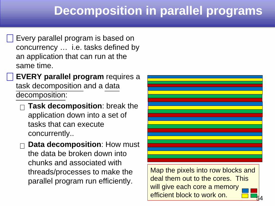
Every parallel program is based on concurrency … i.e. tasks defined by an application that can run at the same time.
EVERY parallel program requires a task decomposition and a data decomposition:
Task decomposition: break the application down into a set of tasks that can execute concurrently..
Data decomposition: How must the data be broken down into chunks and associated with threads/processes to make the parallel program run efficiently.
55
Map the pixels into row blocks and deal them out to the cores. This will give each core a memory efficient block to work on.
Decomposition in parallel programs
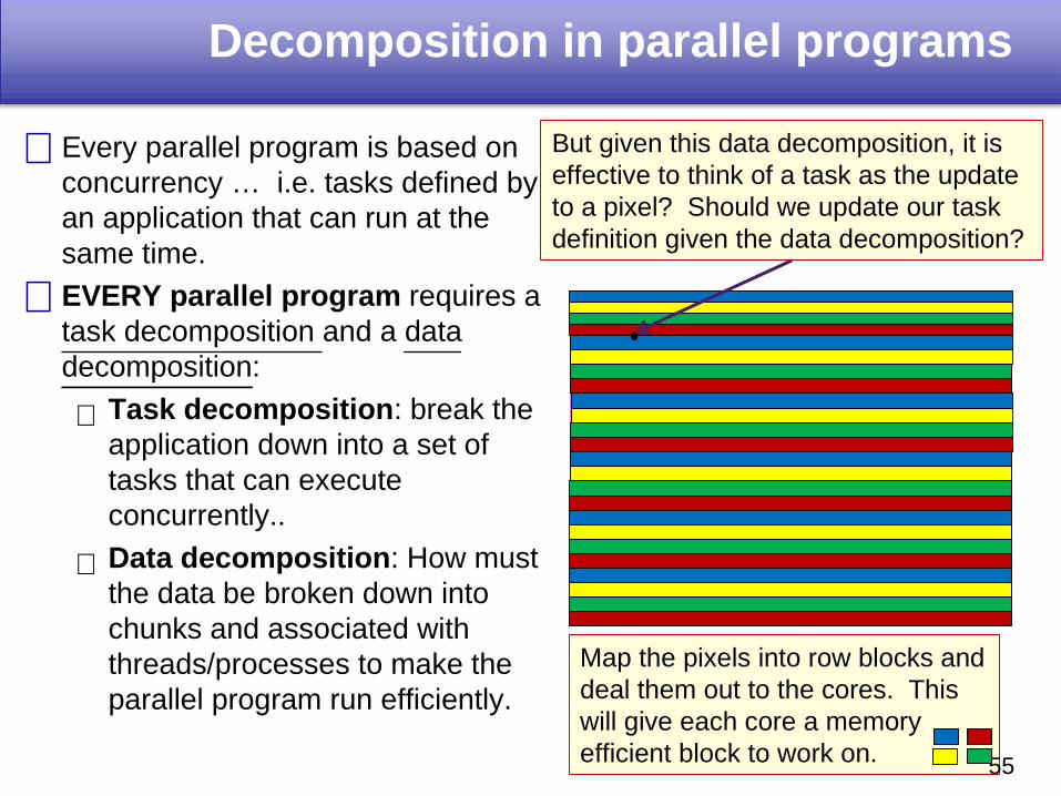
Every parallel program is based on concurrency … i.e. tasks defined by an application that can run at the same time.
EVERY parallel program requires a task decomposition and a data decomposition:
But given this data decomposition, it is effective to think of a task as the update to a pixel? Should we update our task definition given the data decomposition?
Task decomposition: break the application down into a set of tasks that can execute concurrently..
Data decomposition: How must the data be broken down into chunks and associated with threads/processes to make the parallel program run efficiently.
56
Map the pixels into row blocks and deal them out to the cores. This will give each core a memory efficient block to work on.
Decomposition in parallel programs
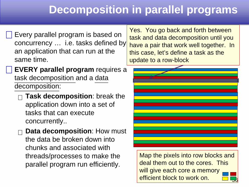
Every parallel program is based on concurrency … i.e. tasks defined by an application that can run at the same time.
EVERY parallel program requires a task decomposition and a data decomposition:
Yes. You go back and forth between task and data decomposition until you have a pair that work well together. In this case, let’s define a task as the update to a row-block
Task decomposition: break the application down into a set of tasks that can execute concurrently..
Data decomposition: How must the data be broken down into chunks and associated with threads/processes to make the parallel program run efficiently.
Outline
• High Performance computing: A hardware system view
• The processors in HPC systems
• Parallel Computing: Basic Concepts
• The Fundamental patterns of parallel Computing
58
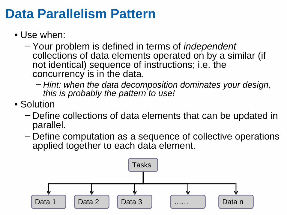
Data Parallelism Pattern
• Use when:– Your problem is defined in terms of independent
collections of data elements operated on by a similar (if not identical) sequence of instructions; i.e. the concurrency is in the data. – Hint: when the data decomposition dominates your design,
this is probably the pattern to use!• Solution
– Define collections of data elements that can be updated in parallel.
– Define computation as a sequence of collective operations applied together to each data element.
Data 1 Data 2 Data 3 Data n
Tasks
……
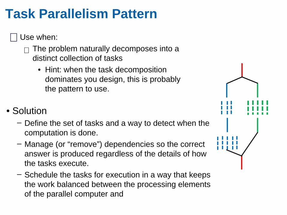
Task Parallelism Pattern
• Solution– Define the set of tasks and a way to detect when the
computation is done.– Manage (or “remove”) dependencies so the correct
answer is produced regardless of the details of how the tasks execute.
– Schedule the tasks for execution in a way that keeps the work balanced between the processing elements of the parallel computer and
Use when:
The problem naturally decomposes into a distinct collection of tasks
• Hint: when the task decomposition dominates you design, this is probably the pattern to use.
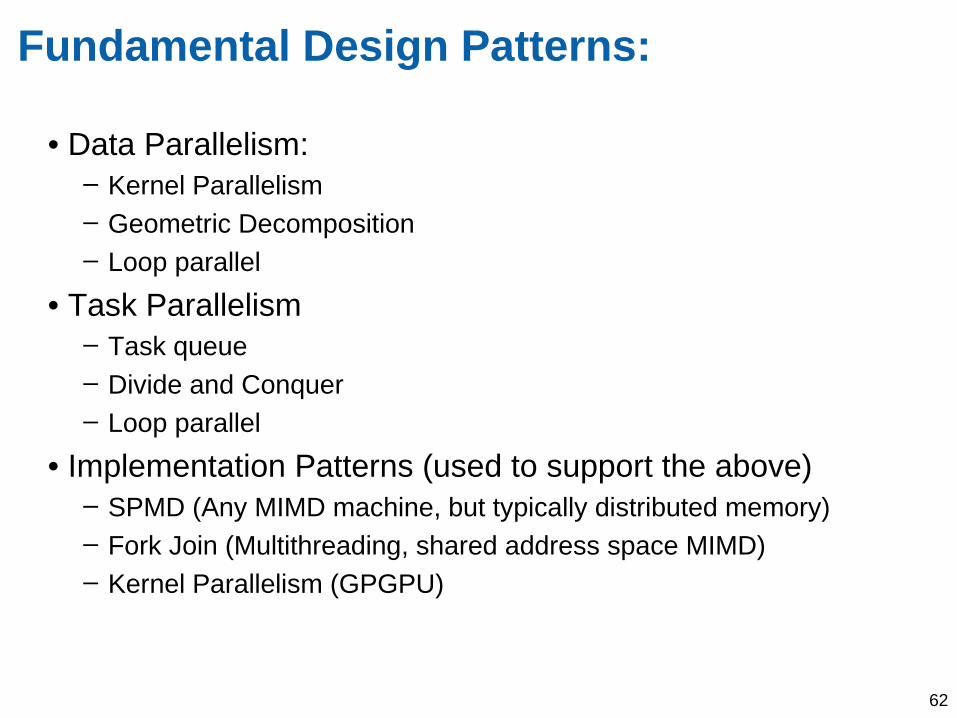
Fundamental Design Patterns:
• Data Parallelism:– Kernel Parallelism– Geometric Decomposition– Loop parallel
• Task Parallelism– Task queue– Divide and Conquer– Loop parallel
• Implementation Patterns (used to support the above)– SPMD (Any MIMD machine, but typically distributed memory)– Fork Join (Multithreading, shared address space MIMD)– Kernel Parallelism (GPGPU)
62
Summary Processors with lots of cores/vector-units/SIMT connected into clusters are here to stay. You
have no choice … embrace parallel computing!
Protect your software investment … refuse
to use any programming model that locks you to a vendors platform.
Open Standards are the ONLY rational
approach in the long run.
Parallel programming can be intimidating to learn, but there are only 6 fundamental design patterns used in
most programs