ORNL/TM-2016/173

Parallel Execution of Functional Mock-up Units in Buildings Modeling

Ozgur Ozmen James J. Nutaro Joshua R. New June 30, 2016 Approved for public release.

Distribution is unlimited.

DOCUMENT AVAILABILITY Reports produced after January 1, 1996, are generally available free via US Department of Energy (DOE) SciTech Connect. Website http://www.osti.gov/scitech/ Reports produced before January 1, 1996, may be purchased by members of the public from the following source: National Technical Information Service 5285 Port Royal Road Springfield, VA 22161 Telephone 703-605-6000 (1-800-553-6847) TDD 703-487-4639 Fax 703-605-6900 E-mail info@ntis.gov Website http://www.ntis.gov/help/ordermethods.aspx Reports are available to DOE employees, DOE contractors, Energy Technology Data Exchange representatives, and International Nuclear Information System representatives from the following source: Office of Scientific and Technical Information PO Box 62 Oak Ridge, TN 37831 Telephone 865-576-8401 Fax 865-576-5728 E-mail reports@osti.gov Website http://www.osti.gov/contact.html

This report was prepared as an account of work sponsored by an agency of the United States Government. Neither the United States Government nor any agency thereof, nor any of their employees, makes any warranty, express or implied, or assumes any legal liability or responsibility for the accuracy, completeness, or usefulness of any information, apparatus, product, or process disclosed, or represents that its use would not infringe privately owned rights. Reference herein to any specific commercial product, process, or service by trade name, trademark, manufacturer, or otherwise, does not necessarily constitute or imply its endorsement, recommendation, or favoring by the United States Government or any agency thereof. The views and opinions of authors expressed herein do not necessarily state or reflect those of the United States Government or any agency thereof.

ORNL/TM-2016/173

Energy & Transportation Science Division Computing and Computational Sciences Division

PARALLEL EXECUTION OF FUNCTIONAL MOCK-UP UNITS IN BUILDINGS MODELING

Ozgur Ozmen James J. Nutaro Joshua R. New

Date Published: June 30, 2016

Prepared by OAK RIDGE NATIONAL LABORATORY

Oak Ridge, Tennessee 37831-6283 managed by

UT-BATTELLE, LLC for the

US DEPARTMENT OF ENERGY under contract DE-AC05-00OR22725

iii

CONTENTS

Page

CONTENTS ................................................................................................................................................. iiiLIST OF FIGURES ....................................................................................................................................... vLIST OF TABLES ...................................................................................................................................... viiACRONYMS ................................................................................................................................................ ixACKNOWLEDGMENTS ............................................................................................................................ xiABSTRACT ................................................................................................................................................... 11. INTRODUCTION .................................................................................................................................. 12. MULTI-TANK PROBLEM ................................................................................................................... 2

2.1 IMPLEMENTATION VERIFICATION ..................................................................................... 22.2 SIMULATION TIME AND FMUS ON TWO CORES .............................................................. 42.3 SINGLE FMU VS. MULTIPLE FMUS ...................................................................................... 42.4 PARALLEL SPEEDUP ............................................................................................................... 6

3. MODELICA BUILDINGS LIBRARY .................................................................................................. 83.1 A ROOM MODEL WITH THREE COMPONENTS ................................................................. 83.2 SIMULATION RUNTIME PERFORMANCE OF THE ROOM MODEL .............................. 103.3 VERIFICATION OF THE HYBRID SOLVER FOR THE FOUR-ROOM MODEL .............. 133.4 SIMULATION RUNTIME PERFORMANCE OF THE FOUR-ROOM MODEL .................. 13

4. FUTURE RESEARCH ON DISAGGREGATION ............................................................................. 145. CONCLUSIONS .................................................................................................................................. 15APPENDIX A. CODE REPOSITORY ................................................................................................... A-1Appendix A. CODE REPOSITORY ....................................................................................................... A-3

v

LIST OF FIGURES

Figure Page

Figure 1. This depiction shows the physical layout of the standard multi-tank mixing problem being

used here as a test system model. ............................................................................................... 2Figure 2. Tank-1 liquid levels are nearly identical across C++ implementation via 1 FMU, via 2

FMUs, and the OpenModelica (Euler) solver. ........................................................................... 3Figure 3. Tank-2 liquid levels are nearly identical across C++ implementation via 1 FMU, via 2

FMUs, and the OpenModelica (Euler) solver. ........................................................................... 3Figure 4. Runtimes when going to two cores for different simulation lengths and number of FMUs

shows greatest speedup via parallelization of the solver loops. ................................................. 4Figure 5. Simulation runtimes (in seconds) for a 200-tank system as a function of the number of

FMUs shows significant increases around 25 FMUs. ................................................................ 5Figure 6. Total runtimes (in seconds), including simulation, for a 200-tank system as a function of

the number of FMUs shows an optimal runtime around 25 FMUs for this mixed-tank problem. ...................................................................................................................................... 5

Figure 7. Comparison of a 200-tank model in 200 FMUs across multiple cores shows total runtimes (in seconds) do not speed up linearly due to the costly creation of FMUs. ............................... 6

Figure 8. Comparison of a 200-tank model in 200 FMUs across multiple cores shows simulation runtime (in seconds), which is less than the 200TF1 system simulation runtime (red line) without parallelization. ...................................................................................................... 6

Figure 9. Running a 200-tank model as a function of the number of FMUs on four compute cores shows simulation runtimes (in seconds) that originates from load balancing. ........................... 7

Figure 10. A thermal zone with outside temperature, conductivity of the walls, sensor, mixed air, and heat capacitance. Inlet and Outlet ports allow connections to other system components. ................................................................................................................................ 8

Figure 11. A fan with cooling coil, mixed air, and water source and sink. They constitute the cooling system. Input u is the air mass flow rate decided by the controller. ............................. 9

Figure 12. A controller that controls the mass flow of the water source that flows into the cooling coil in the cooling system. Input u is the room temperature. ..................................................... 9

Figure 13. Whole room model representing couplings of control, cooling system, and the thermal zone. ......................................................................................................................................... 10

Figure 14. Simulation runtime (in seconds) of the three component room model across multiple cores shows limited performance benefits up to three compute cores. .................................... 11

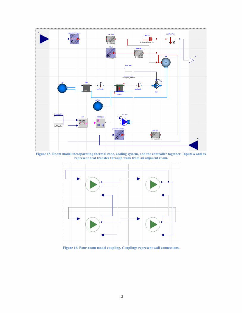
Figure 15. Room model incorporating thermal zone, cooling system, and the controller together. Inputs u and u1 represent heat transfer through walls from an adjacent room. ....................... 12

Figure 16. Four-room model coupling. Couplings represent wall connections. .......................................... 12Figure 17. Four-room model temperature values for each room generated via the C++ wrapper and

the hybrid solver. ...................................................................................................................... 13Figure 18. Four-room model temperature values for each room generated via the Dymola (Euler)

solver. ....................................................................................................................................... 13Figure 19. Simulation runtime (in seconds) comparison of the four-room model on different

numbers of compute cores. Comparison against Dymola runtime of the Figure 16 system shows significantly less simulation runtime which is better than Dymola runtime. .................................................................................................................................... 14

vii

LIST OF TABLES

Table Page

ix

ACRONYMS

FMI Functional Mock-up Interface FMU Functional Mock-up Unit OpenMP Open Multi-Processing XML eXtensible Markup Language API Application Programming Interface

x

xi

ACKNOWLEDGMENTS

Funding for this project was provided by field work proposal CEBT105 under Department of Energy Building Technology Activity Number BT0310000. This manuscript has been authored by UT-Battelle, LLC, under Contract Number DEAC05-00OR22725 with DOE. The United States Government retains and the publisher, by accepting the article for publication, acknowledges that the United States Government retains a non-exclusive, paid-up, irrevocable, world-wide license to publish or reproduce the published form of this manuscript, or allow others to do so, for United States Government purposes.

xii

1

ABSTRACT

A Functional Mock-up Interface (FMI) defines a standardized interface to be used in computer simulations to develop complex cyber-physical systems. FMI implementation by a software modeling tool enables the creation of a simulation model that can be interconnected, or the creation of a software library called a Functional Mock-up Unit (FMU). This report describes an FMU wrapper implementation that imports FMUs into a C++ environment and uses an Euler solver that executes FMUs in parallel using Open Multi-Processing (OpenMP). The purpose of this report is to elucidate the runtime performance of the solver when a multi-component system is imported as a single FMU (for the whole system) or as multiple FMUs (for different groups of components as sub-systems). This performance comparison is conducted using two test cases: (1) a simple, multi-tank problem; and (2) a more realistic use case based on the Modelica Buildings Library. In both test cases, the performance gains are promising when each FMU consists of a large number of states and state events that are wrapped in a single FMU. Load balancing is demonstrated to be a critical factor in speeding up parallel execution of multiple FMUs.

1. INTRODUCTION

There are three major technologies used for the findings included in this report: (i) Modelica, (ii) Functional Mock-up Interface (FMI), and (iii) Open Multi-Processing (OpenMP). Modelica1 is a non-proprietary and object-oriented modeling language that is created to ease the modeling of complex cyber-physical systems. Its advantage is related to its acausal and equation-based nature that allows modelers to focus on the structure of the system being modeled rather than transformations related to the numerical solver. It is widely adopted in various domains (e.g., automobile manufacturing, power electronics, and building simulation). FMI2 is a tool-independent standard to describe models using eXtensible Markup Language (XML) files and compiled C code. There are currently more than 70 tools that support import or export features using the standard, and adoption is increasing. The standard aims to support model exchange (without solver only the model) and co-simulation (exchanged including the native solver) of dynamic models. It allows users to share models across simulation tools by either solving the models using the native solvers of the target platform (i.e., model exchange) or wrapping the solver from the source platform (i.e., co-simulation). In either case, the package that is transferred between the source and target platform is called a Functional Mock-up Unit (FMU). OpenMP3 is an application programming interface (API) that supports shared-memory multiprocessing programming in C, C++, and Fortran.

In this report, we describe import/export features of FMUs supported by an FMU wrapper that enables execution of FMUs in C++. This wrapper is capable of creating an FMU instance in C++ with all function pointers and state variables for the purpose of evaluating runtime performance gains from parallel execution of FMUs. The workflow is as follows. First, a model is developed in Modelica and its FMUs are exported using OpenModelica4 or a similar Modelica compiler. Next, the FMUs are imported using the wrapper, coupled via input and output variables, and solved via Euler solver in parallel using OpenMP. This process and performance results are discussed in the context of two test cases.

1 https://www.modelica.org 2 https://www.fmi-standard.org 3 http://openmp.org/wp/ 4 https://www.openmodelica.org

2

2. MULTI-TANK PROBLEM

In the first experimental setup, multiple tanks are connected in serial. While the first tank is continuously receiving a constant flow of liquid, each tank drains at a specified rate proportional to the liquid level into the adjacent tank, i.e.,

𝑑𝑥𝑑𝑡

= −𝑎𝑥 + 𝑢 where 𝑥 is the liquid level, u is the input flow from the preceding tank, and 𝑎 is the time constant that represents the geometry and physics of fluid flow to the succeeding tank. Figure 1 illustrates the whole system where X is the liquid level, i is the tank index, and N is the total number of tanks.

Figure 1. This depiction shows the physical layout of the standard multi-tank mixing problem being used here as a test

system model.

The FMU wrapper and the Euler solver implementations allow users to define the number of tanks that will form an FMU and the number of FMUs users want to couple together. For example, if there is a 200-tank system, then it can be solved by forming a single FMU incorporating 200 tanks, two FMUs each consisting of 100 tanks, and so on. This problem allows an easy way to decompose a large system in a load-balanced manner to determine performance tradeoffs as a function of number of FMUs.

2.1 IMPLEMENTATION VERIFICATION

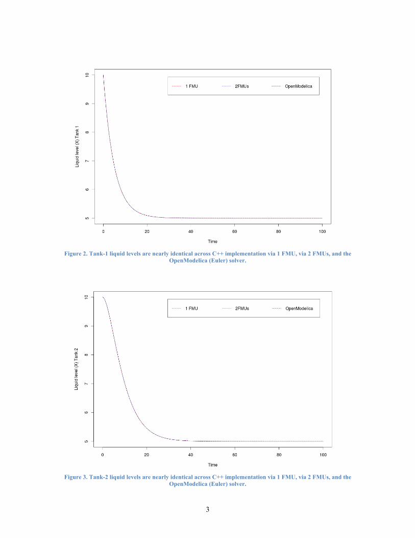
To ensure the FMU wrapper and Euler solver are implemented correctly, a two-tank system is created and solutions acquired from the implemented Euler solver and the OpenModelica Euler solver are compared between a 1-FMU and 2-FMU models. As can be seen in Figure 2 and Figure 3, solutions for liquid levels in Tank 1 and Tank 2 are nearly identical up to three decimal points.

3

Figure 2. Tank-1 liquid levels are nearly identical across C++ implementation via 1 FMU, via 2 FMUs, and the

OpenModelica (Euler) solver.

Figure 3. Tank-2 liquid levels are nearly identical across C++ implementation via 1 FMU, via 2 FMUs, and the

OpenModelica (Euler) solver.

4

2.2 SIMULATION TIME AND FMUS ON TWO CORES

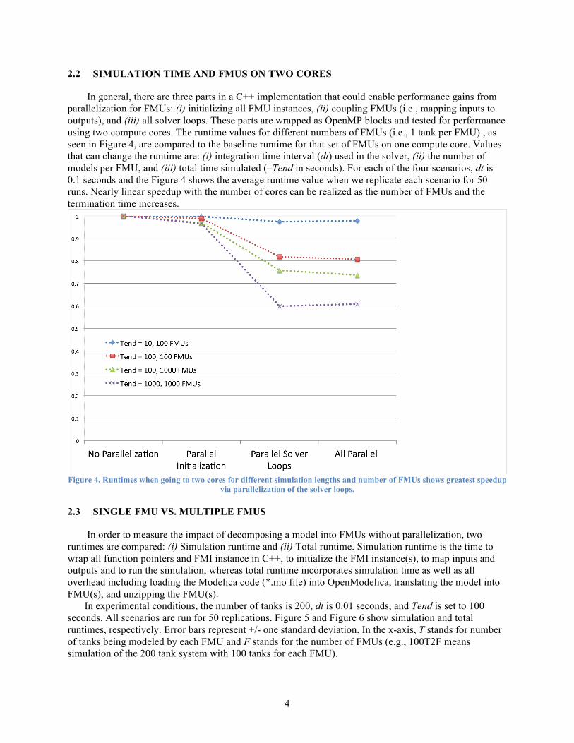
In general, there are three parts in a C++ implementation that could enable performance gains from parallelization for FMUs: (i) initializing all FMU instances, (ii) coupling FMUs (i.e., mapping inputs to outputs), and (iii) all solver loops. These parts are wrapped as OpenMP blocks and tested for performance using two compute cores. The runtime values for different numbers of FMUs (i.e., 1 tank per FMU) , as seen in Figure 4, are compared to the baseline runtime for that set of FMUs on one compute core. Values that can change the runtime are: (i) integration time interval (dt) used in the solver, (ii) the number of models per FMU, and (iii) total time simulated (–Tend in seconds). For each of the four scenarios, dt is 0.1 seconds and the Figure 4 shows the average runtime value when we replicate each scenario for 50 runs. Nearly linear speedup with the number of cores can be realized as the number of FMUs and the termination time increases.

Figure 4. Runtimes when going to two cores for different simulation lengths and number of FMUs shows greatest speedup

via parallelization of the solver loops.

2.3 SINGLE FMU VS. MULTIPLE FMUS

In order to measure the impact of decomposing a model into FMUs without parallelization, two runtimes are compared: (i) Simulation runtime and (ii) Total runtime. Simulation runtime is the time to wrap all function pointers and FMI instance in C++, to initialize the FMI instance(s), to map inputs and outputs and to run the simulation, whereas total runtime incorporates simulation time as well as all overhead including loading the Modelica code (*.mo file) into OpenModelica, translating the model into FMU(s), and unzipping the FMU(s).

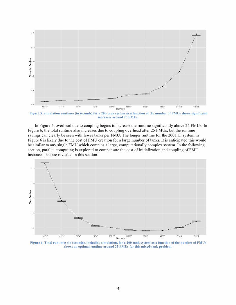
In experimental conditions, the number of tanks is 200, dt is 0.01 seconds, and Tend is set to 100 seconds. All scenarios are run for 50 replications. Figure 5 and Figure 6 show simulation and total runtimes, respectively. Error bars represent +/- one standard deviation. In the x-axis, T stands for number of tanks being modeled by each FMU and F stands for the number of FMUs (e.g., 100T2F means simulation of the 200 tank system with 100 tanks for each FMU).

5

Figure 5. Simulation runtimes (in seconds) for a 200-tank system as a function of the number of FMUs shows significant

increases around 25 FMUs.

In Figure 5, overhead due to coupling begins to increase the runtime significantly above 25 FMUs. In Figure 6, the total runtime also increases due to coupling overhead after 25 FMUs, but the runtime savings can clearly be seen with fewer tanks per FMU. The longer runtime for the 200T1F system in Figure 6 is likely due to the cost of FMU creation for a large number of tanks. It is anticipated this would be similar to any single FMU which contains a large, computationally complex system. In the following section, parallel computing is explored to compensate the cost of initialization and coupling of FMU instances that are revealed in this section.

Figure 6. Total runtimes (in seconds), including simulation, for a 200-tank system as a function of the number of FMUs

shows an optimal runtime around 25 FMUs for this mixed-tank problem.

6

2.4 PARALLEL SPEEDUP

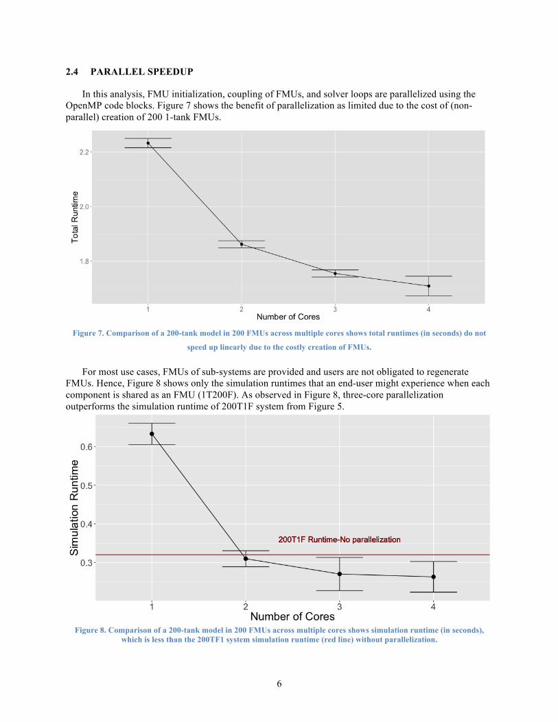
In this analysis, FMU initialization, coupling of FMUs, and solver loops are parallelized using the OpenMP code blocks. Figure 7 shows the benefit of parallelization as limited due to the cost of (non-parallel) creation of 200 1-tank FMUs.

Figure 7. Comparison of a 200-tank model in 200 FMUs across multiple cores shows total runtimes (in seconds) do not

speed up linearly due to the costly creation of FMUs.

For most use cases, FMUs of sub-systems are provided and users are not obligated to regenerate FMUs. Hence, Figure 8 shows only the simulation runtimes that an end-user might experience when each component is shared as an FMU (1T200F). As observed in Figure 8, three-core parallelization outperforms the simulation runtime of 200T1F system from Figure 5.

Figure 8. Comparison of a 200-tank model in 200 FMUs across multiple cores shows simulation runtime (in seconds),

which is less than the 200TF1 system simulation runtime (red line) without parallelization.

7

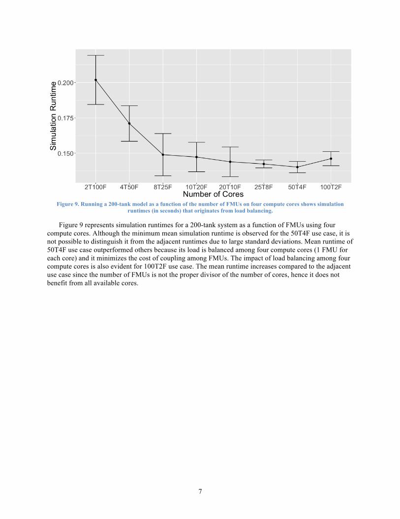
Figure 9. Running a 200-tank model as a function of the number of FMUs on four compute cores shows simulation

runtimes (in seconds) that originates from load balancing.

Figure 9 represents simulation runtimes for a 200-tank system as a function of FMUs using four compute cores. Although the minimum mean simulation runtime is observed for the 50T4F use case, it is not possible to distinguish it from the adjacent runtimes due to large standard deviations. Mean runtime of 50T4F use case outperformed others because its load is balanced among four compute cores (1 FMU for each core) and it minimizes the cost of coupling among FMUs. The impact of load balancing among four compute cores is also evident for 100T2F use case. The mean runtime increases compared to the adjacent use case since the number of FMUs is not the proper divisor of the number of cores, hence it does not benefit from all available cores.

8

3. MODELICA BUILDINGS LIBRARY

In the first experimental setup, there is a complete control on the number of components (tanks) within each FMU and the whole multi-tank system assuming that the system incorporates multiple instances of the same components connected in serial. However, the component models are more complex and developed as a whole entity in real use cases. To explore performance of disaggregated models, multiple test cases are developed leveraging the Modelica Buildings Library5 that includes complex component models developed for buildings modeling.

3.1 A ROOM MODEL WITH THREE COMPONENTS

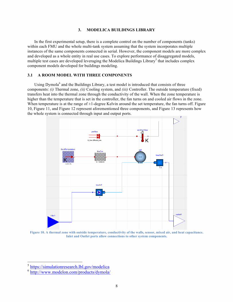
Using Dymola6 and the Buildings Library, a test model is introduced that consists of three components: (i) Thermal zone, (ii) Cooling system, and (iii) Controller. The outside temperature (fixed) transfers heat into the thermal zone through the conductivity of the wall. When the zone temperature is higher than the temperature that is set in the controller, the fan turns on and cooled air flows in the zone. When temperature is at the range of ±1-degree Kelvin around the set temperature, the fan turns off. Figure 10, Figure 11, and Figure 12 represent aforementioned three components, and Figure 13 represents how the whole system is connected through input and output ports.

Figure 10. A thermal zone with outside temperature, conductivity of the walls, sensor, mixed air, and heat capacitance.

Inlet and Outlet ports allow connections to other system components.

5 https://simulationresearch.lbl.gov/modelica 6 http://www.modelon.com/products/dymola/

9

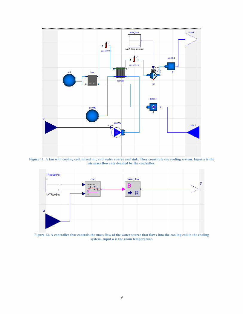
Figure 11. A fan with cooling coil, mixed air, and water source and sink. They constitute the cooling system. Input u is the

air mass flow rate decided by the controller.

Figure 12. A controller that controls the mass flow of the water source that flows into the cooling coil in the cooling

system. Input u is the room temperature.

10

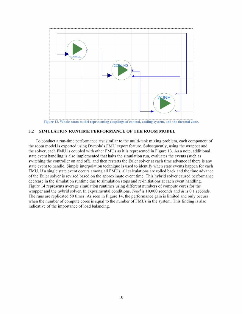
Figure 13. Whole room model representing couplings of control, cooling system, and the thermal zone.

3.2 SIMULATION RUNTIME PERFORMANCE OF THE ROOM MODEL

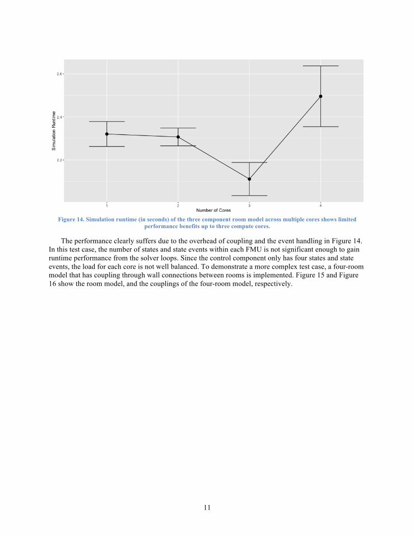
To conduct a run-time performance test similar to the multi-tank mixing problem, each component of the room model is exported using Dymola’s FMU export feature. Subsequently, using the wrapper and the solver, each FMU is coupled with other FMUs as it is represented in Figure 13. As a note, additional state event handling is also implemented that halts the simulation run, evaluates the events (such as switching the controller on and off), and then restarts the Euler solver at each time advance if there is any state event to handle. Simple interpolation technique is used to identify when state events happen for each FMU. If a single state event occurs among all FMUs, all calculations are rolled back and the time advance of the Euler solver is revised based on the approximate event time. This hybrid solver caused performance decrease in the simulation runtime due to simulation stops and re-initiations at each event handling. Figure 14 represents average simulation runtimes using different numbers of compute cores for the wrapper and the hybrid solver. In experimental conditions, Tend is 10,000 seconds and dt is 0.1 seconds. The runs are replicated 50 times. As seen in Figure 14, the performance gain is limited and only occurs when the number of compute cores is equal to the number of FMUs in the system. This finding is also indicative of the importance of load balancing.

11

Figure 14. Simulation runtime (in seconds) of the three component room model across multiple cores shows limited

performance benefits up to three compute cores.

The performance clearly suffers due to the overhead of coupling and the event handling in Figure 14. In this test case, the number of states and state events within each FMU is not significant enough to gain runtime performance from the solver loops. Since the control component only has four states and state events, the load for each core is not well balanced. To demonstrate a more complex test case, a four-room model that has coupling through wall connections between rooms is implemented. Figure 15 and Figure 16 show the room model, and the couplings of the four-room model, respectively.

12

Figure 15. Room model incorporating thermal zone, cooling system, and the controller together. Inputs u and u1

represent heat transfer through walls from an adjacent room.

Figure 16. Four-room model coupling. Couplings represent wall connections.

13

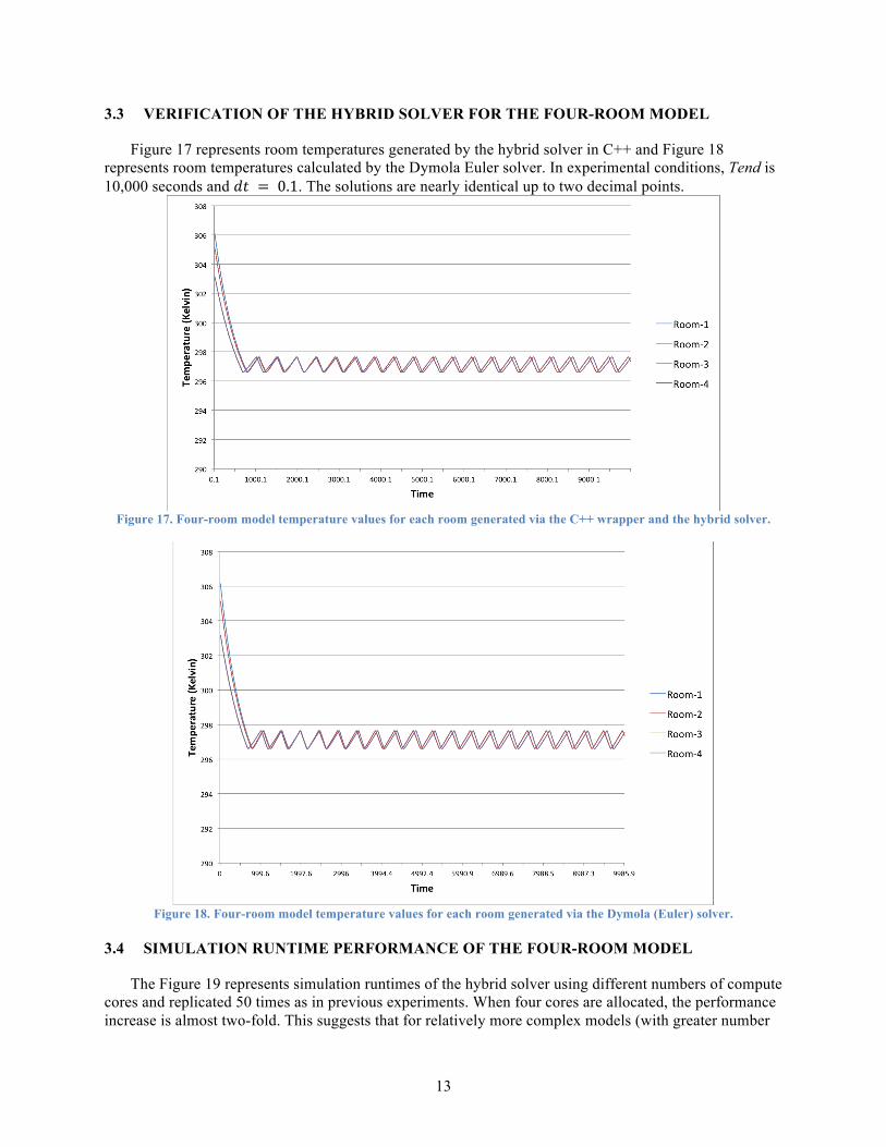
3.3 VERIFICATION OF THE HYBRID SOLVER FOR THE FOUR-ROOM MODEL

Figure 17 represents room temperatures generated by the hybrid solver in C++ and Figure 18 represents room temperatures calculated by the Dymola Euler solver. In experimental conditions, Tend is 10,000 seconds and 𝑑𝑡 = 0.1. The solutions are nearly identical up to two decimal points.

Figure 17. Four-room model temperature values for each room generated via the C++ wrapper and the hybrid solver.

Figure 18. Four-room model temperature values for each room generated via the Dymola (Euler) solver.

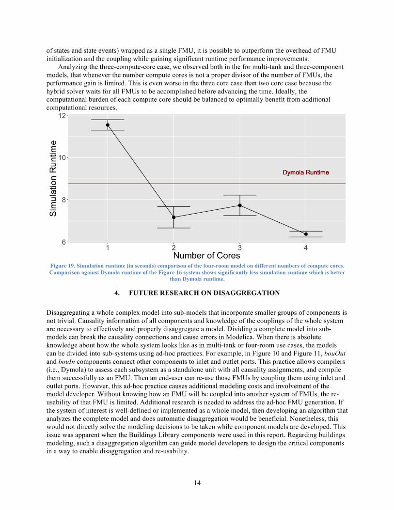
3.4 SIMULATION RUNTIME PERFORMANCE OF THE FOUR-ROOM MODEL

The Figure 19 represents simulation runtimes of the hybrid solver using different numbers of compute cores and replicated 50 times as in previous experiments. When four cores are allocated, the performance increase is almost two-fold. This suggests that for relatively more complex models (with greater number

14

of states and state events) wrapped as a single FMU, it is possible to outperform the overhead of FMU initialization and the coupling while gaining significant runtime performance improvements.

Analyzing the three-compute-core case, we observed both in the for multi-tank and three-component models, that whenever the number compute cores is not a proper divisor of the number of FMUs, the performance gain is limited. This is even worse in the three core case than two core case because the hybrid solver waits for all FMUs to be accomplished before advancing the time. Ideally, the computational burden of each compute core should be balanced to optimally benefit from additional computational resources.

Figure 19. Simulation runtime (in seconds) comparison of the four-room model on different numbers of compute cores. Comparison against Dymola runtime of the Figure 16 system shows significantly less simulation runtime which is better

than Dymola runtime.

4. FUTURE RESEARCH ON DISAGGREGATION

Disaggregating a whole complex model into sub-models that incorporate smaller groups of components is not trivial. Causality information of all components and knowledge of the couplings of the whole system are necessary to effectively and properly disaggregate a model. Dividing a complete model into sub-models can break the causality connections and cause errors in Modelica. When there is absolute knowledge about how the whole system looks like as in multi-tank or four-room use cases, the models can be divided into sub-systems using ad-hoc practices. For example, in Figure 10 and Figure 11, bouOut and bouIn components connect other components to inlet and outlet ports. This practice allows compilers (i.e., Dymola) to assess each subsystem as a standalone unit with all causality assignments, and compile them successfully as an FMU. Then an end-user can re-use those FMUs by coupling them using inlet and outlet ports. However, this ad-hoc practice causes additional modeling costs and involvement of the model developer. Without knowing how an FMU will be coupled into another system of FMUs, the re-usability of that FMU is limited. Additional research is needed to address the ad-hoc FMU generation. If the system of interest is well-defined or implemented as a whole model, then developing an algorithm that analyzes the complete model and does automatic disaggregation would be beneficial. Nonetheless, this would not directly solve the modeling decisions to be taken while component models are developed. This issue was apparent when the Buildings Library components were used in this report. Regarding buildings modeling, such a disaggregation algorithm can guide model developers to design the critical components in a way to enable disaggregation and re-usability.

15

5. CONCLUSIONS

There is a trade-off between the cost of FMU translation for the whole system, and the costs of creating and coupling multiple FMU instances of the system components. In the first test case (multi-tank system), this trade-off is clear from Figure 6 and Figure 7 as different numbers of FMUs scale to different number of cores. If the total runtime (wall clock time) is considered as the primary performance measure, the multi-tank test case suggests decomposing the models into 8 tanks per FMU. This determination of optimal decomposition into FMUs is typically much more difficult for real-world problems.

Parallel computing allows a system modeler to compensate for the cost of initializing FMU instances and coupling processes as shown in Figure 8. Consequently, when FMUs are provided for the system components, coupling the FMUs and solving them in parallel can achieve faster simulation runtimes than solving the whole system as a single FMU via native solvers such as OpenModelica or Dymola.

To test against more complex and realistic test cases, a three-component room model (Figure 13) was developed using the Buildings Library. Additional event-handling is implemented within the Euler solver in C++. Figure 14 shows that improper load balancing of CPU-cores is a major limiter for runtime performance gains. Therefore, the room model is packaged as a whole FMU and multiple rooms are connected in the four-room model (Figure 16). In this case, parallelization across four cores beat the overhead of FMI initialization and coupling (Figure 19) and achieves even faster runtimes than Dymola.

The cost of implementing and coupling the models in Dymola and C++ are neglected in this report, which focuses solely on runtime performance. The cost of modeling becomes more apparent when disaggregation of models is needed. Clear documentation of models, how they were constructed, and practical experience regarding their use is currently essential to effectively decomposing these models. Future research on automatic disaggregation of Modelica models is recommended. A successful disaggregation algorithm would enhance reusability of Buildings Library components as FMUs without additional modeling efforts. Use of parallel execution of FMUs derived from the Buildings library would enable running complex models (with thousands of states and state events) as hundreds of FMUs distributed over hundreds of compute cores. As revealed in the analysis of this report, this approach could cut runtime in half using four computer cores. Leveraging more compute cores and implementing optimizations in the solver have potential to achieve more runtime benefits for more complex problems.

APPENDIX A. CODE REPOSITORY

A-3

APPENDIX A. CODE REPOSITORY

The repository includes all the C++ code, Modelica models, and Python scripts (to parse XMLs) that are used in this report. To acquire access to the repository, please contact Ozgur Ozmen from ozmeno@ornl.gov indicating your e-mail address. If you are a user from ORNL (Oak Ridge National Laboratory), please indicate your UCAMS username in the e-mail. README files in each folder explain how to set up the experiments conducted in this report. The repository is: https://code.ornl.gov/FMI-Modelica/parallelFMI.git