Embed Size (px)
Citation preview

Parallel expected improvements for global optimization:summary, bounds and speed-upTechnical report
OMD2 deliverable Nmbr. 2.1.1-B
Janis Janusevskis · Rodolphe Le Riche ·David Ginsbourger
Abstract The sequential sampling strategies based on Gaussian processes are widely
used for optimization of time consuming simulators. In practice, such computation-
ally demanding problems are solved by increasing number of processing units. This
has therefore induced extensions of sampling criteria which consider the framework of
parallel calculation.
This report further studies expected improvement criteria for parallel and asyn-
chronous computations. A unified parallel asynchronous expected improvement crite-
rion is formulated. Bounds and strategies for comparing criteria values at various design
points are discussed. Finally, the impact of the number of available computing units
on the performance is empirically investigated.
Keywords Kriging based optimization · Gaussian process · Expected improvement ·Optimization using computer grids · Distributed calculations · Monte Carlo
optimization
1 Introduction
Many design problems are nowadays based on computationally costly simulator codes.
The current technology for adressing computationally intensive tasks is based on an
increasing number of processing units (processors, cores, CPUs, GPUs). For example,
Janis JanusevskisLSTI / CROCUS teamEcole Nationale Superieure des Mines de Saint-EtienneSaint-Etienne, FranceE-mail: [email protected]
Rodolphe Le RicheCNRS UMR 5146 and LSTI / CROCUS teamEcole Nationale Superieure des Mines de Saint-EtienneSaint-Etienne, FranceE-mail: [email protected]
David GinsbourgerUniversity of BernBern, SwitzerlandE-mail: [email protected]

2
the next generation of exascale computers (1018 floating point operations per second)
should have of the order of 109 computing nodes [13]. Distributing calculations on
several nodes is particularly relevant in optimization where a natural parallelization
level exists, that of calculating concurrent designs in parallel. However, most current
optimization methods have been thought sequentially. Today, there is a need for opti-
mization strategies that operate within the framework of heterogeneous parallel com-
putation, i.e. algorithms designed for being used on computing grids.
The Efficient Global Optimization (EGO) algorithm [8] has become a popular
choice for optimizing computationally expensive simulation models. EGO is based on
kriging (Gaussian process regression) metamodels, that allow to formulate the Ex-
pected improvement (EI) criterion, which provides a compromise between global ex-
ploration of the domain space and local exploitation of the best known solutions. At
each optimization step the EI is maximized to obtain the next simulation point. By
definition the EI is a sequential one point strategy [5] and lacks means for efficiently
accounting for parallel processing capabilities.
The EI criterion has been adapted for parallel computation in [6],[12] leading to
the so called “q steps EI” (qEI), that provides the synchronous selection of q new
points for the next simulation run. This qEI criterion assumes that the computation
time is constant for all design points, i.e. once a set of points is sent for simulation
the results are available at the same time for all the points in the set. In general this
assumption may not be correct. The simulations at different points may have different
algorithmic complexities or run on nodes with different performances or loads, therefore
the simulations will finish successively, i.e. new computing nodes become available
asynchronously.
The selection of points for the next calculation should be made as soon as compu-
tational resources are available, i.e. asynchronously. In [4] the qEI criterion has been
extended and the so called “Expected Expected Improvement” (EEI) criterion has
been proposed. In the framework of Gaussian processes one assumes that the simu-
lator response at busy points (points that have been sent to simulator but have not
returned yet) are conditional Gaussian random variables. Maximizing expectation of
the EI with respect to busy points allows selection of a new set of points accounting
for the points that are being simulated.
As already noted in [6] and [4], the implementation of these criteria faces several
problems. Firstly, in general qEI and EEI can not be obtained analytically. They should
instead be estimated using numerical procedures such as Monte Carlo (MC). Secondly,
selecting the next point in EGO is a global maximization of the EI problem which
has the same dimension as the design variables. In contrast, maximizing qEI and EEI
has for dimension the number of the design variables multiplied by the number of new
points (the number of free computing nodes). Therefore brute optimization of qEI and
EEI using simple MC may not be cost effective. These problems have been partially
addressed in [6], [4], [1] by introducing heuristics.
This report further studies expected improvement criteria for parallel and asyn-
chronous computational environments. Firstly, the EI(µ,λ) criterion is formulated in a
more general form. Secondly, in section 4, bounds on EI(µ,λ) are provided in section 3
and strategies for comparing EI(µ,λ) at various design points are discussed. Finally,
the impact of the number of available computing units, λ, on the performance, i.e., the
method speed-up, is investigated in section 5.

3
2 A unified presentation of parallel expected improvements
The traditional improvement in the objective value [8], [9] at point x is defined as
I(ω)(x) = max(0, fmin −min(Y(ω))) =(fmin −min(Y(ω))
)+(1)
where fmin = min(Y) is the minimum of the observations, x is the new point for
the next simulation and Y(ω) =(Y(ω)(x)
)|Y is the joint Gaussian vector (kriging
metamodel) at the point of interest x conditioned on the past observations X,Y.
The multi-points improvement [6] can be rewritten as
I(λ)(ω)
(x) = max(0, fmin −min(Yλ(ω))) =
(fmin −min(Yλ
(ω)))+
(2)
where fmin = min(Y) is the minimum of the previous observations, x = (x1, ..., xλ) are
the λ new points for the next simulation and Yλ(ω) = (Y1, ..., Yλ) =
(Y(ω)(x1), ..., Y(ω)(xλ)
)|Y
is joint Gaussian vector (kriging metamodel) at the new points x = (x1, ..., xλ) condi-
tioned on the past observations X,Y.
The multi-points asynchronous improvement is defined as
I(µ,λ)(ω)
(x) = max(0,min(fmin,Yµ(ω)
)−min(Yλ(ω))) =
(min(fmin,Y
µ(ω)
)−min(Yλ(ω))
)+(3)
where fmin = min(Y) is the minimum of the previous observations, x = (xµ+1, ..., xµ+λ)
are the λ points for the next simulation and
Yλ(ω) = (Yµ+1, ..., Yµ+λ) =
(Y(ω)(xµ+1), ..., Y(ω)(xµ+λ)
)|Y is again the Gaussian vec-
tor at the points of interest conditioned on the past observations X,Y, and
Yµ(ω)
= (Y1, ..., Yµ) =(Y(ω)(x1), ..., Y(ω)(xµ)
)|Y is the joint Gaussian vector at the
points where the simulator has not yet provided responses (i.e., the busy points). The
multi-points asynchronous improvement has first been introduced in [4], [3]. As it can
be readily seen from eq. (3), it is a natural measure of the progress made between
points being or already calculated (the min(fmin,Yµ(ω)
) term) and future points (the
min(Yλ(ω)) term). It has an important feature for asynchronous parallel calculation: it
is null at the busy points. Indeed,
If min(Yµ(ω)
) ≤ fmin , I(µ,λ)(ω)
(x) =(
min(Yµ(ω)
)−min(Yµ(ω)
))+
= 0
else min(Yµ(ω)
) > fmin , I(µ,λ)(ω)
(x) =(fmin −min(Yµ
(ω)))+
= 0
When used in the context of optimization, a natural choice for the sampling crite-
rion is to use the expectation of the improvement, thus for multi-points asynchronous
improvement in eq. (3) we have
EI(µ,λ)(x) = EΩ(I(µ,λ)(ω)
(x)). (4)
In the special case when µ = 0 and λ = 1, it reduces to classical EI, with a
known analytical expression. When µ = 0 and λ ≥ 2, it is equivalent to the qEI
and we will further write it as EI(λ) (note that for µ = 0 and λ = 2, an analytical
expression is given in [6]). Note also that by applying the law of total expectations

4
eq. (4) is equivalent to EEI [4]. In general calculating eq. (4) amounts to estimating
a multidimensional integral (where the number of dimensions depends on the number
of available and busy nodes) with respect to Gaussian density and must be based on
numerical procedures, in particular MC methods.
MC based estimation procedure samples the Gaussian vector (Yλ,Yµ) and esti-
mates the criteria values. Even though the calculation of the improvement (eq. (2) and
eq. (3)) is not complex, the estimation of the criteria may become time consuming.
The error of MC estimate depends on the number of samples, which may be large if a
high precision of the estimate is needed. Such cases are very likely to occur at the end
of the optimization when the points x proposed by the mainly converged optimizer are
close to each other. Additionally, the crude MC sampling becomes inefficient with the
number of EGO iterations because the probability of improvement becomes small.
2.1 Illustration of criteria
For illustrating the criteria we use the one dimensional test function
y = sin(3x)− exp
(− (x+ 0.1)2
0.01
). (5)
The test function together with predicted kriging mean and 2σMC confidence intervals,
one point EI, 2 points EI or EI(0,2) and 2 points asynchronous EI or EI(1,2) are shown
in fig. 1. It can be well seen that the criteria are symmetrical with respect to the line
x1 = x2. Also notice that the maximum of EI(0,2)(x) is close to x = (x1, x2) where
(x1, x2) corresponds to the modes of EI(x).
The points obtained from maxEI(λ) for several iterations are shown in fig. 2. In
this case of ’deceptive’ function, the region of the true optimum is located faster with
increasing λ. Larger λ values induce a better exploration of the design space allowing
construction of a globally more accurate regression model and thus preventing EI from
stagnation.
Figure 3 provides an example of points created through maxEI(1,1) for 3 iterations
(6 time steps), assuming that calculation of the objective takes two time steps, and
that the second computing node becomes available after one time step.
3 EI(µ,λ) criteria bounds
In this section upper and lower bounds for the criteria of eq. (4) are derived. Firstly,
in section 3.1, we address the parallel case EI(λ) and after, in section 3.2, we look at
the asynchronous case EI(µ,λ).
3.1 Bounds on the multipoints expected improvement
From the definition of multi-points improvement
I(λ)(ω)
(x) = max(0, fmin −min(Y1, ..., Yλ))
≥ max(0, fmin − Yi) = I(λ=1)(ω)
(xi)

5
(a) Test function eq. (5) (dashed), krigingmodel based on 5 observations - predicted mean(blue), 2σ predicted confidence intervals (red).
(b) One point EI, EI(x).
(c) Contour lines of 2 points EI, EI(0,2)(x) (d) 3D plot of 2 points EI, EI(0,2)(x)
(e) Contour lines of 2 points async. EI (busy
point xbusy = −0.34), EI(1,2)(x)
(f) 3D plot of 2 points async. EI (busy point
xbusy = −0.34), EI(1,2)(x)
Fig. 1: Illustrations of the simple, the two-points and the two-points asynchronous
Expected Improvements using the analytical test function eq. (5). EI(0,2) and EI(1,2)
are calculated with 10000 MC simulations. Notice the maximum of EI(0,2)(x) is close
to x = (x1, x2) where (x1, x2) corresponds to the modes of EI(x).

6
Fig. 2: Example of points generated by maxEI(λ) (red) at different iterations, true
function (solid line), points used for kriging model (blue). First line λ = 1, second line
λ = 2, third line λ = 3, forth line λ = 4. First column – first iteration, second column
– second iteration, third column – third iteration. For the first iteration θ = 0.3, for
iterations 2 and 3, θ is estimated by maximizing the kriging model likelihood.
Fig. 3: Example of points generated by maxEI(1,1) during 6 time steps. It is assumed
that calculation of the objective takes two time steps. Objective function (solid line),
points used for kriging model (blue), points where the response value has been calcu-
lated (red), busy points (sent for calculation but not known yet – green). Initially and
after the first time step θ = 0.3, for subsequent steps (after data arrives) θ is estimated
by maximizing the kriging model likelihood.
and therefore the lower bound on multi-points EI is
EI(λ)(x) ≥ maxi=1,λ
EI(λ=1)(xi). (6)

7
The upper bound on the expectation of multi-points improvement can also be
derived from its definition
EI(λ)(ω)
(x) = E[max(0, fmin −min(Y1, ..., Yλ))] (7)
=
λ∑i=1
∫ fmin
−∞
∫ +∞
yi
. . .
∫ +∞
yi
(fmin − yi) fN (µ,Σ)(y1, ..., yλ)(dyj)j 6=i dyi
≤λ∑i=1
∫ fmin
−∞
∫ +∞
−∞. . .
∫ +∞
−∞(fmin − yi) fN (µ,Σ)(y1, ..., yλ)(dyj)j 6=i dyi
=
λ∑i=1
∫ fmin
−∞(fmin − yi)
∫ +∞
−∞. . .
∫ +∞
−∞fN (µ,Σ)(y1, ..., yλ)(dyj)j 6=i dyi
=
λ∑i=1
∫ fmin
−∞(fmin − yi)fN (µi,σ2
i )(yi)dyi
=
λ∑i=1
EI(λ=1)(xi) (8)
where fN (µ,Σ) is the density of a multivariate normal distribution with mean µ and
covariance matrix Σ, (dyj)j 6=i is the sequence from dy1 to dyλ except dyi.
The above relations provide the upper bound
EI(λ)(x) ≤λ∑i
EI(λ=1)(xi). (9)
The plots in fig. 4 show upper and lower bounds versus EI(λ) (λ = 2) for 100
random points. The test case is the same as in the previous example of fig. 1 with the
function eq. (5). EI(λ) is calculated using 100 and 10000 MC simulations. It can be
seen that for these points bounds are seemingly tight.
3.2 Bounds on the asynchronous multi-points expected improvement
From the definition of asynchronous multi-points improvement, one has
I(µ,λ)(ω)
(x) = max(0,min(fmin, Yµ1 , ..., Y
µµ )−min(Y λ1 , ..., Y
λλ )) (10)
≤
max(0, fmin −min(Y λ1 , ..., Y
λλ ))
max(0, Y µi −min(Y λ1 , ..., Yλλ ))
(11)
and the expectation is
EI(µ,λ)(ω)
(x) = ≤
E[max(0, fmin −min(Y λ1 , ..., Y
λλ ))] = EI
(λ)(ω)
(x)
E[max(0, Y µi −min(Y λ1 , ..., Yλλ ))]
(12)
If we define
I∗(i,j)(ω)
(x) = max(0, Y µi − Yλj ) (13)

8
(a) Upper bound versus EI(λ) with estimated
2σ confidence intervals. EI(λ) estimated using100 MC samples.
(b) Upper bound versus EI(λ) with estimated
2σ confidence intervals. EI(λ) estimated using10000 MC samples.
(c) Lower bound versus EI(λ) with estimated
2σ confidence intervals. EI(λ) estimated using100 MC samples.
(d) Lower bound versus EI(λ) with estimated
2σ confidence intervals. EI(λ) estimated using10000 MC samples.
Fig. 4: Upper and lower bounds versus EI(λ) (λ = 2) for random chosen points with
2σ confidence intervals. The test case is based on eq. (5) as in fig. 1. EI(λ) is calculated
using 100 and 10000 MC simulations. Notice that for the points in this example bounds
are seemingly tight.
and
EI∗(i,j)(x) = EΩ(I∗(i,j)(ω)
(x)) (14)
then using a similar reasoning as in eq. (7) one can say that
E[max(0, Y µi −min(Y λ1 , ..., Yλλ ))] ≤
λ∑j=1
EI∗(i=1,j)(xj). (15)
The upper bound is
9
EI(µ,λ)(x) ≤ min
λ∑j
EI(λ=1)(xj),
λ∑j
EI∗(i=1,j)(xj), ...,
λ∑j
EI∗(i=µ,j)(xj)
.
(16)
Notice that all components on the right hand side of eq. (16) have analytical expressions
since Y µi Yλj | Y is Gaussian with mean and variance known from kriging.
To estimate the lower bound on the asynchronous expected improvement one can
write
I(µ,λ)(ω)
(x) = max(0,min(fmin, Yµ1 , ..., Y
µµ )−min(Y λ1 , ..., Y
λλ ))
= max(0,min(fmin, Yµ1 , ..., Y
µµ )− Y λ1 , ...,min(fmin, Y
µ1 , ..., Y
µµ )− Y λλ )
≥ (min(fmin, Yµ1 , ..., Y
µµ )− Y λj )+.
The expectations of type E[(min(fmin, Yµ1 , ..., Y
µµ )− Y λj )+] are again integrals on
the Rµ+1 hyperspace truncated by several hyperplanes. As noted previously, the esti-
mation of such integrals is based on numerical procedures and are not trivial. Instead
a trivial lower bound of the asynchronous expected improvement from the definition
of the improvement can be used
EI(µ,λ)(x) ≥ 0. (17)
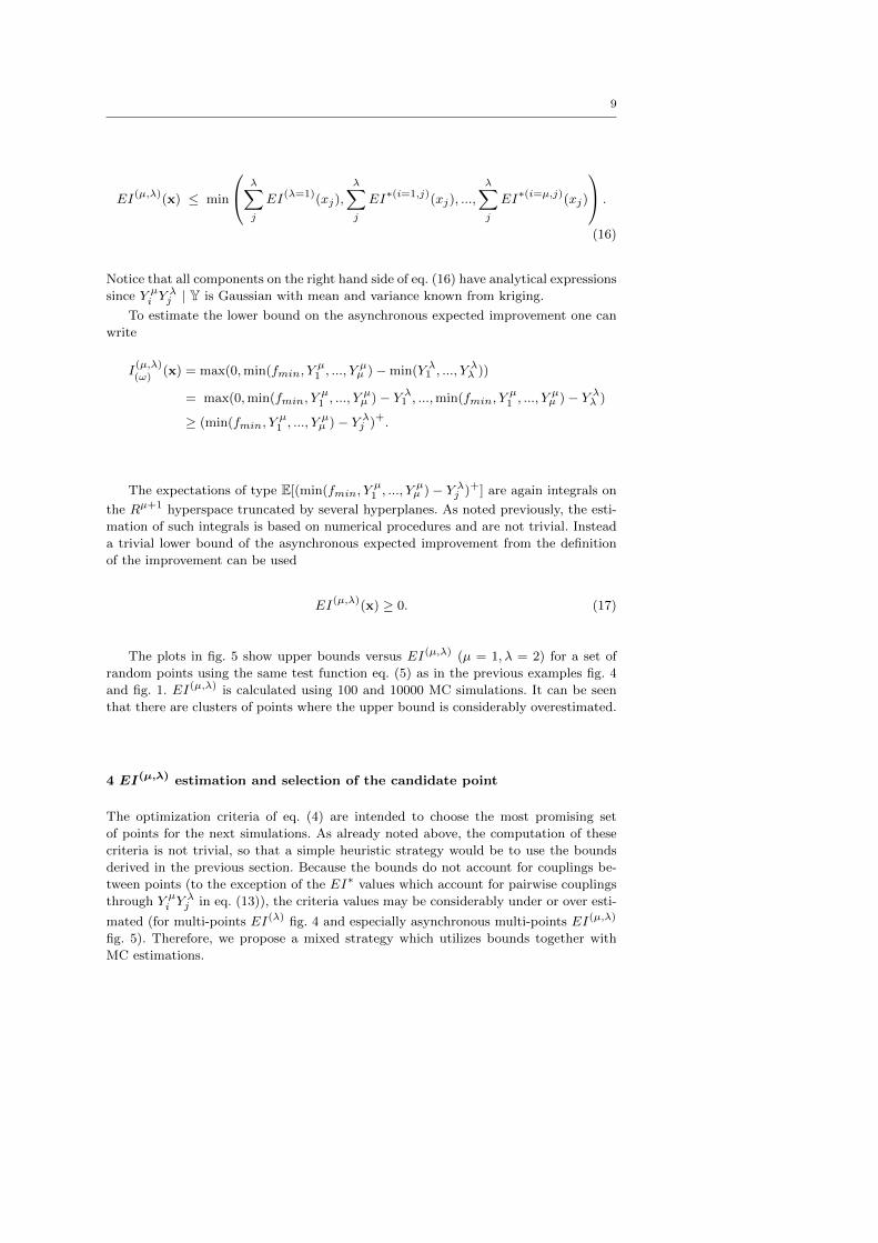
The plots in fig. 5 show upper bounds versus EI(µ,λ) (µ = 1, λ = 2) for a set of
random points using the same test function eq. (5) as in the previous examples fig. 4
and fig. 1. EI(µ,λ) is calculated using 100 and 10000 MC simulations. It can be seen
that there are clusters of points where the upper bound is considerably overestimated.
4 EI(µ,λ) estimation and selection of the candidate point
The optimization criteria of eq. (4) are intended to choose the most promising set
of points for the next simulations. As already noted above, the computation of these
criteria is not trivial, so that a simple heuristic strategy would be to use the bounds
derived in the previous section. Because the bounds do not account for couplings be-
tween points (to the exception of the EI∗ values which account for pairwise couplings
through Y µi Yλj in eq. (13)), the criteria values may be considerably under or over esti-
mated (for multi-points EI(λ) fig. 4 and especially asynchronous multi-points EI(µ,λ)
fig. 5). Therefore, we propose a mixed strategy which utilizes bounds together with
MC estimations.

10
(a) Upper bound versus EI(µ,λ) for 100 randompoints with estimated 2σ confidence intervals.EI(µ,λ) estimates using 100 MC samples.
(b) Upper bound versus EI(µ,λ) for 1000 ran-
dom points. EI(λ) estimates using 10000 MCsamples.
(c) Lower bound (diamond), upper bound
(square), estimated EI(µ,λ) (red dot) with es-timated 2σ confidence intervals (red lines) on
100 random points. EI(µ,λ) estimates using 10MC samples.
(d) Lower bound (diamond), upper bound
(square), estimated EI(µ,λ) (red dot) with es-timated 2σ confidence intervals (red lines) on
100 random points. EI(µ,λ) estimates using 100MC samples.
Fig. 5: Upper and lower bounds, EI(µ,λ) (µ = 1, λ = 2) for 100 and 1000 random points
with 2σ confidence intervals. The test case is based on eq. (5) like in fig. 1. EI(µ,λ) is
calculated using 100 and 10000 MC simulations. Notice in this example that for many
points the upper bounds are overestimated.
4.1 Estimation and confidence intervals
The MC estimation allows us to estimate the expectations of improvements in eq. (4).
By using crude MC the estimated EI(µ,λ) (denoted in this section as EI) is
EIMC(x) =1
n
N∑i=1
I(ω)(x)
where N is the number of samples and I(ω)(x) is the improvement calculated from
the sampled trajectory of the conditional Gaussian process at the points of interest.

11
“Points” has a plural here because, as the reader may remember, in the case of the par-
allel asynchronous expected improvement, expectation is calculated over joint random
variables located at µ+ λ points in the optimization variable space.
The error variance of this estimate also can be estimated from data as
σ2MC =1
n(n− 1)
N∑i=1
(I(ω)(x)− EIMC)2.
Therefore (EIMC |EI) follows Student’s t-distribution with mean EI and variance σ2MC
with n − 1 degrees of freedom. Bounds discussed in previous chapter provide us with
prior information on EI. Lets assume that α ≤ EI ≤ β and EI uniformly distributed
between its bounds, EI ∼ U(α, β). Using Bayes theorem it is possible to show that
(EI|EIMC) follows a truncated Student’s t-distribution
p(EI|EIMC) =p(EIMC |EI)p(EI)∫ +
− p(EIMC |EI)p(EI)dEI(18)
=1
σMCfν
(EI − EIMC
σMC
)[Fν
(α− EIMC
σMC
)− Fν
(β − EIMC
σMC
)]−1(19)
where Fν(.) and fν(.) are the c.d.f. and p.d.f. of the Student’s t- variable with ν = n−1
degrees of freedom. The moments of truncated t-distribution are given for example in
[10] and the formulas are copied in appendix A. Numerical tests have shown that these
formulas become numerically unstable as the bounds are on the same side and far from
the mean.
However it is also know that as ν increases the t-distribution is well approximated
by the Gaussian distribution. The density function of truncated Gaussian distribution is
equivalent to eq. (18) except that instead of Fν(.) and fν(.) we have Φ(.) and φ(.) which
are the c.d.f. and p.d.f. of the standard normal distribution. The mean and variance of
truncated Gaussian random are known and if we denote by u1 = (α − EIMC)/σMC
and u2 = (β − EIMC)/σMC , then
E(EI|EIMC) = EIMC +φ(u1)− φ(u2)
Φ(u2)− Φ(u1)σMC (20)
and
VAR(EI|EIMC) = σ2MC
[1 +
u1φ(u1)− u2φ(u2)
Φ(u2)− Φ(u1)−(φ(u1)− φ(u2)
Φ(u2)− Φ(u1)
)2]. (21)
The [E(EI|EIMC) − k√VAR(EI|EIMC),E(EI|EIMC) + k
√VAR(EI|EIMC)]
when k = 1 gives a 68% confidence that EI is inside this interval.
12
4.2 Ranking of candidate points
The confidence intervals from the previous section allow to compare two points. Let
say that we have a set of points xi, i = 1..n , MC estimates EIMC(xi) and σ2MC(xi),
let’s denote by µi = E(EI|EIMC(xi)) and σi =√VAR(EI|EIMC(xi)) .
Now, with over 60% confidence (k = 1),
if µi − kσi ≥ µj + kσj then EI(xi) ≥ EI(xj) (22)
if µi + kσi < µj − kσj then EI(xi) < EI(xj). (23)
If neither eq. (22) nor eq. (23) hold then we do not have enough information to
safely discriminate between the two points and additional data is necessary. In order
to reduce the confidence intervals N = Ni +Nj additional MC samples are computed,
where Ni and Nj are the number of samples at points xi and xj , respectively. A simple
strategy is to add a number of samples proportional to the variance of the estimate,
Ni =σ∗iN
σ∗i + σ∗j, Nj = N −Ni
where σ∗i = σi, σ∗j = σj , if σMC(xi) > 0, σMC(xj) > 0.
Special care must be taken when none of the MC samples actually obtains tra-
jectory where improvement is positive. In such cases the σMC = 0 and EIMC = 0
are underestimated. On the other hand increasing number of total MC samples with
no hits (trajectory providing positive improvement) indicates that true value of EI is
small. To safely discriminate between two candidate points one needs to account for
such situations.
If point xj has no MC hit but xi has at least one sample where improvement is posi-
tive it is possible to estimate the improvement variance σ2MC(xi) and use this variance
to overestimate the improvement variance at the other point xj as Ni/Njσ2MC(xi),
where Ni and Nj are the number of already computed MC samples.Therefore if σi > 0
and σj = 0 then σ∗i = σi and σ∗j is calculated using eq. (21) where σMC(xj) =
σMC(xi)√
ninj
.
However if no MC samples have positive improvement at both points .i.e. σMC(xi) =
0, σMC(xj) = 0 then the number of samples should be increased equally Ni = Nj =
N/2, until the probability of improvement is small and we can assume that the true
value of EI at both points is very small and further sampling is unnecessary, or until
the MC budget is exceeded.
4.3 Illustration of the impact of bounds
In fig. 6 we show the 80th percentile of the number of MC simulations versus λ for
comparing random pairs of points. For each λ setting, 100 random trajectories of
Gaussian process are generated (and act as sample functions), the kriging models are
built from 4 evenly spaced points using the same covariance form as that used in the
process generation.
For each trajectory a pair of points is randomly selected (i.e., a set of µ points and
two sets of λ points) and their EI(µ,λ) values are compared using MC based procedures

13
with and without bounds. The initial number of MC samples is 10 and at each step
N = 20. The maximum number of MC samples for each point is limited to 105. If more
MC samples are necessary one concludes that for the two points values of EI(µ,λ) are
very similar and the points cannot be compared. The percentiles in fig. 6 are computed
only on points that can be compared. For test cases where µ = 0, on the average 99
pairs of points where comparable within this number of maximum MC evaluations. For
cases where µ = 1 and µ = 3, on the average only 75 and 69 pairs where comparable.
The results indicate that the bounds reduce the necessary number of MC evalu-
ations, however (especially in asynchronous case µ > 0), the discrimination of points
often requires a very large number of MC evaluations. Furthermore, in practice one is
interested in selecting points with maximum EI(µ,λ): the optimization of EI(µ,λ) even-
tually leads to regions where the values of EI(µ,λ) become similar and a much larger
number of MC simulations are needed for the ranking of points i.e., the non compa-
rable cases occur more often. Therefore the strategy based on mixing crude MC with
bounds is effective only at the initial optimization steps when the global exploration
of EI(µ,λ) resembles random sampling.
(a) µ = 0. Sample trajectories generated on1000 point grid with Matern 5/2 kernel and θ =0.3.
(b) µ = 0. Sample trajectories generated on1000 point grid with Matern 5/2 kernel and θ =0.15.
(c) µ = 1. Sample trajectories generated on1000 point grid with Matern 5/2 kernel andθ = 0.3.
(d) µ = 3. Sample trajectories generated on1000 point grid with Matern 5/2 kernel and θ =0.3.
Fig. 6: 80th percentile of the number of MC simulations necessary to discriminate be-
tween EI(µ,λ) at two random points versus λ. The number of MC simulations without
bounds (dashed line), number of MC simulations with bounds (solid line).

14
5 An empirical study of EI(0,λ) scale-up properties
To empirically compare the efficiency of the parallel improvement criteria (eq. (4)) to
classical EI, we use random test functions in one dimension, i.e. we sample Gaussian
process trajectories on a 1000 point grid using Matern 5/2 kernel functions [11] with
fixed scaling parameters θ = 0.3 (fig. 8, fig. 10) and θ = 0.15 (fig. 9, fig. 11 ).
5.1 Optimization strategy
For the maximization of EI(λ)(x), we use the Covariance Matrix Adaptation Evolu-
tion Strategy algorithm (CMA-ES, [7]) with some changes. Firstly, as we have data
only at discrete locations, every point sampled by CMA-ES is mapped to the nearest
grid point. Secondly, the ranking of points in a given population is based on the com-
parison procedure described in section 4. This MC based ranking makes the objective
function noisy, which is compatible with the stochastic CMA-ES algorithm, but adds
randomness in the tests.
When comparing two points xi and xj (two sets of points in actual space) which
have close EI values (for example the points are close to each other) the necessary
number of MC simulations for safe comparison may be very large. In order to keep
the optimization procedure computationally feasible, the maximum number of MC
simulation for estimating EI at one point is 105. If the numbers of MC simulations
for both points exceed this budget, we assume that it is not possible to discriminate
between the two points (as explained in section 4) because their criteria values are very
close. This situation occurs during the optimization, especially towards the end of the
CMA-ES iterations, when the variance of the population is small. Furthermore, the
values of EI (and probability of improvement) decreases with the number of iterations.
This further increases the number of MC samples needed to discriminate between two
points, as most of the sampled trajectories will be above the best observed point. These
problems illustrate the necessity for more efficient criteria estimation procedures (such
as MC variance reduction techniques), where more trajectories that are interesting for
calculating the criteria ( below the best point) are used.
5.2 Results
The impact of λ on the speed-up of the parallel expected improvements is examined
by comparing the actual improvements (difference between best objective values at the
points of the initial DOE and at the λ points provided by criteria) after one time step.
The assumption is made that the simultaneous calculation of the objective is possible
on multiple computing nodes, however the actual number of utilized processors depends
on the criterion, i.e. EI(1) provides one new point, EI(2) two new points, etc.
The variation in actual improvement due to the EI optimization strategy is il-
lustrated in fig. 7, where 10 runs of EI maximization are performed on a single test
trajectory fig. 7a and the mean actual improvement with 1σ confidence bounds fig. 7c
and mean improvement rank together with 1σ confidence fig. 7d. The improvement
rank is obtained for each trajectory by ordering the best actual improvement values
with respect to λ. It is used as a normalization method for better visualization of the
speed-up related to parallel EIs.

15
(a) Sample trajectory on 1000 point gridwith Matern 5/2 kernel and θ = 0.3.
(b) Actual improvement of EI(λ) for 10independent maximizations, λ = 1...4.
(c) Actual mean improvement, 1σ confi-
dence intervals of EI(λ), λ = 1...4.
(d) Mean improvement rank, 1σ confidence in-
tervals of EI(λ), λ = 1...4.
Fig. 7: Variation in actual improvement due to the stochastic maximization of EI(λ).
Statistics calculated for 10 runs on a fixed test function.
The mean improvement, mean rank with confidence intervals for actual improve-
ment on 10 random test functions (fig. 8a and fig. 9a) at points of maxxEI(λ)(x)
are illustrated in fig. 8c and fig. 9c. The initial kriging model is built using 4 evenly
spaced points and the covariance hyper-parameter θ is fixed equal to the value used in
trajectory generation. The results of this test indicate that the EI(λ) has a sub-linear
improvement with respect to λ.
The λ impact on improvement is also studied in a more realistic scenario, where
points of maximum EI are added sequentially to the DOE as they would during an
optimization. The following typical three steps optimization strategy is investigated :
1. the kriging model is built from 4 initial points;
2. kriging covariance parameters are not known a priori and are estimated by maxi-
mizing likelihood;
3. EI(λ)(x) is maximized by CMA-ES;
4. the λ points together with f(x) are added to the DOE.
Steps 2, 3, 4 are repeated for 2 iterations.
The statistics of the overall best improvement (the best improvement after three
iterations with respect to initial 4 point DOE) versus λ over 10 random test functions
using the three step optimization strategy are shown in fig. 10 and fig. 11. As in the
previous cases, the results suggest that the EI(λ) provides a sub-linear improvement
with respect to λ.

16
(a) Sample trajectories on 1000 point grid with Matern 5/2 kernel and θ = 0.3.
(b) Actual mean improvement over 10 trajectories for λ = 1...4.
(c) Mean improvement rank, 1σ confidence intervals over 10 trajectories forλ = 1...4.
Fig. 8: λ impact on performance observed on 10 relatively smooth (θ = 0.3) random
functions

17
(a) Sample trajectories on 1000 point grid with Matern 5/2 kernel and θ = 0.15.
(b) Actual mean improvement over 10 trajectories for λ = 1...4.
(c) Actual average improvement over 10 trajectories for λ = 1...4.
Fig. 9: λ impact on performance observed on 10 shaky (θ = 0.15) random functions

18
(a) Sample trajectories on 1000 point grid with Matern 5/2 kernel and θ = 0.3.
(b) Actual mean overall improvement after 3 iterations, over 10 randomtrajectories, λ = 1...4.
(c) Mean overall improvement rank, 1σ confidence intervals over 10 randomtrajectories, λ = 1...4.
Fig. 10: λ impact on performance observed on 10 relatively smooth (θ = 0.3) random
functions over 3 iterations.

19
(a) Sample trajectories on 1000 point grid with Matern 5/2 kernel and θ = 0.15.
(b) Actual mean overall improvement after 3 iterations, over 10 randomtrajectories, λ = 1...4.
(c) Mean overall improvement rank, 1σ confidence intervals over 10 randomtrajectories, λ = 1...4.
Fig. 11: λ impact on performance observed on 10 shaky (θ = 0.15) random functions
over 3 iterations.
20
6 Conclusion
In this study, the EI(µ,λ) criterion has been formulated by combining parallel and
asynchronous versions of the expected improvement criterion. EI(µ,λ) measures the
expected improvement brought by λ new points when the value of the objective function
at µ already chosen points is not yet known but will be.
Bounds on EI(µ,λ) have been provided for use in MC based estimation and com-
parison strategy. The easily calculable bounds may be useful at the initial steps of
EI(µ,λ) maximization when comparing points at distant locations and the coupling
between design points is weak.
Finally, the effect of the number of available nodes, λ, on the optimization perfor-
mance has been investigated in 1D test cases. The results indicate that parallel EIs
provide sub-linear speed-up. The observed speed-up is in agreement with the intuition
that the ability to obtain points in parallel should provide better and perhaps ”safer”
results. Note that in the test cases studied here the actual type of kriging covariance
kernel is known. It seems, however, that in general the parallel calculation of λ points
provides better exploration of the design space. Therefore it may partially solve the
problem of deceptive functions [8],[2]. Better exploration of the design space allows
globally more accurate construction of kriging models and therefore reduces the risk
of stagnating searches in local regions due to deceptive initial states.
The implementation of the EI(µ,λ)(x) for optimization indicates several difficul-
ties. Firstly, the necessary number of MC simulations increases a lot in order to be able
to discriminate close points. Secondly, crude MC sampling is often inefficient because
trajectories that are better than the best observation become seldom as the optimiza-
tion proceeds. Thirdly, the number of dimensions of x increases proportionally to the
number of nodes. These challenges call for further studies on specialized optimization
heuristics and MC procedures.
References
1. Vincent Dubourg, Bruno Sudret, and Jean-Marc Bourinet. Reliability-based design opti-mization using kriging surrogates and subset simulation. Structural and MultidisciplinaryOptimization, pages 1–18, 2011. 10.1007/s00158-011-0653-8.
2. Alexander I. Forrester and Donald R. Jones. Global optimization of deceptive functionswith sparse sampling. 2008.
3. D. Ginsbourger, J. Janusevskis, R. Le Riche, and C. Chevalier. Dealing with asynchronic-ity in kriging-based parallel global optimization. In Second World Congress on GlobalOptimization in Engineering & Science (WCGO-2011), July 3-7 2011.
4. David Ginsbourger, Janis Janusevskis, and Rodolphe Le Riche. Dealing with asyn-chronicity in parallel Gaussian Process based global optimization. Technical report,July 2010. Deliverable no. 2.1.1-A of the ANR / OMD2 project available as http://hal.archives-ouvertes.fr/hal-00507632.
5. David Ginsbourger and Rodolphe Le Riche. Towards GP-based optimization with finitetime horizon. In Alessandra Giovagnoli, Anthony C. Atkinson, Bernard Torsney, andMay Caterina, editors, mODa 9 Advances in Model-Oriented Design and Analysis, pages89–96. Springer, 2010.
6. David Ginsbourger, Rodolphe Le Riche, and Laurent Carraro. Kriging is well-suited toparallelize optimization. In Yoel Tenne and Chi-Keong Goh, editors, Computational In-telligence in Expensive Optimization Problems, Springer series in Evolutionary Learningand Optimization, pages 131–162. springer, 08 2009.
7. N. Hansen. The CMA evolution strategy: a comparing review. In J.A. Lozano, P. Lar-ranaga, I. Inza, and E. Bengoetxea, editors, Towards a new evolutionary computation.Advances on estimation of distribution algorithms, pages 75–102. Springer, 2006.

21
8. Donald R. Jones. A taxonomy of global optimization methods based on response surfaces.Journal of Global Optimization, 21:345–383, 2001.
9. Donald R. Jones, Matthias Schonlau, and William J. Welch. Efficient global optimizationof expensive black-box functions. Journal of Global Optimization, 13(4):455–492, 1998.
10. Hea-Jung Kim. Moments of truncated student-t distribution. Journal of the KoreanStatistical Society, 37(1):81 – 87, 2008.
11. Carl E. Rasmussen and Christopher K. I. Williams. Gaussian Processes for MachineLearning (Adaptive Computation and Machine Learning). The MIT Press, December2005.
12. Matthias Schonlau. Computer experiments and global optimization. PhD thesis, Waterloo,Ont., Canada, Canada, 1997. AAINQ22234.
13. William JALBY. Scientific directions for exascale computing research. In forum Ter@tech,Palaiseau, France, June 2011. Ecole Polytechnique.
A Moments of Students t-truncated distribution
If we denote by T = (EI − EIMC)/σMCMC and a = (α − EIMC)/σMCMC and b = (β −EIMC)/σMCMC then the moments of truncated t-distribution in interval [a, b] are given forexample in [10] and
E(T ) = Gν(1)(A−(ν−1)/2(ν)
−B−(ν−1)/2(ν)
)
E(T 2) =ν
ν − 2+Gν(1)(aA
−(ν−1)/2(ν)
− bB−(ν−1)/2(ν)
)
where
Gν(l) =Γ ((ν − l)/2)νν/2
2[Fν(b)− Fν(a)]Γ (ν/2)Γ (1/2)
and A(ν) = ν + a2 and B(ν) = ν + b2. In our case
E(EI|EIMC) = EIMC + σMCMCE(T )
andVAR(EI|EIMC) = σ2
MCMC(E(T 2)− E(T )2)