Parallel MATLAB at FSU: PARFOR and SPMDjburkardt/presentations/matlab_parallel... · MATLAB Parallel Computing Introduction PARFOR: a Parallel FOR Loop QUAD Example (PARFOR) ODE Example

Parallel MATLAB at FSU:PARFOR and SPMD

John BurkardtDepartment of Scientific Computing

Florida State University..........

1:30 - 2:30Thursday, 31 March 2011499 Dirac Science Library

..........http://people.sc.fsu.edu/∼jburkardt/presentations/. . .

matlab parallel 2011 fsu.pdf

1 / 75

MATLAB Parallel Computing

Introduction

PARFOR: a Parallel FOR Loop

QUAD Example (PARFOR)

ODE Example (PARFOR)

SPMD: Single Program, Multiple Data

QUAD Example (SPMD)

DISTANCE Example (SPMD)

Conclusion

2 / 75

INTRO: Why Parallel Programming?

Why are we talking about parallel programming in the first place?

Many people have no need for parallel programming.However, that assumes that they are:

satisfied with the speed of their programs (forever!);

not interested in solving problems with larger data sets (ever!);

not interested in rewriting their programs.

At one time, I might also have added:

not willing to buy special parallel hardware,

but most new desktops and laptops contain dual or quadcoreprocessors, it’s not hard to find 12 cores systems, and the numberof cores will increase in the future.

3 / 75

INTRO: MultiCore Requires Parallel Programming

At one time, researchers needing faster execution for biggerproblems simply bought the latest, fastest (sequential) processor.

Supercomputers of the past, such as the legendary series of Craycomputers, were simply enormously expensive machines for feedingand cleaning up after a single really fast and powerful processor.

But the speed of a single processor has reached a permanentceiling of 4 GigaHertz and will never get faster.

4 / 75

INTRO: MultiCore Requires Parallel Programming

To ensure a future for High Performance Computing:

processor manufacturers have developed multicore systems;

network companies created fast interprocessor connections;

research universities have assembled computer clusterscapable of running a single program;

language committees have developed OpenMP and MPI for Cand FORTRAN applications;

researchers have developed new parallel algorithms;

the MathWorks has developed parallel options in MATLAB.

5 / 75

INTRO: Parallel MATLAB

MATLAB’s Parallel Computing Toolbox or PCT runs on a user’sdesktop, and can take advantage of up to 8 cores there.

MATLAB’s Distributed Computing Server controls parallelexecution of a program on a cluster with tens or hundreds of cores.

The FSU HPC facility has a cluster of 526 compute nodes or”processors” controlling 2688 cores; the current license forMATLAB allows a program to run on up to 16 cores simultaneouslythere. (This limit could be increased if demand justified it.)

6 / 75

INTRO: Who Can Access Parallel MATLAB?

Anyone can do simple experiments with parallel MATLAB ontheir own desktop machine (if they have the Parallel ComputingToolbox);

They can do similar experiments on the Scientific ComputingDepartment’s hallway machines, although these only have twocores.

Any FSU researcher can request an account on the FSU HPCsystem, and hence run parallel MATLAB on 16 cores.

7 / 75

INTRO: How Does One Run Parallel MATLAB?

To run parallel MATLAB on your desktop involves:

setting up the run;

supplying a program which includes parallel commands.

and in some cases, both these steps are very simple.

As you can imagine, running on the cluster is a little more involved.

You set up the run by calling a command that submits your job toa queue. For short jobs, you might wait for the results, but forlonger jobs, you actually log out and come back later to get yourresults.

This is one reason why it’s helpful to do initial small experimentson a desktop machine.

8 / 75

INTRO: PARFOR and SPMD

In this talk, I will outline:

two ways to create a parallel program in MATLAB

the process of running a parallel program on desktop machine;

how to run the same program on the FSU HPC cluster.

what kinds of speedup (or slowdowns!) you can expect.

9 / 75

INTRO: PARFOR and SPMD

We will look at two ways to write a parallel MATLAB program:

suitable for loops can be made into parfor loops;

the spmd statement can define cooperating synchronizedprocessing;

parfor approach is a simple way of making FOR loops run inparallel, and is similar to OpenMP.

spmd allows you to design almost any kind of parallelcomputation; it is powerful, but requires rethinking the programand data. It is similar to MPI.

10 / 75


Introduction





QUAD Example (SPMD)


Conclusion

11 / 75

PARFOR: a Parallel FOR Command

parfor is MATLAB’s simplest parallel programming command.

parfor replaces the for command in cases where a loop can beparallelized - (and what does that mean?)

The loop iterations are divided up among different “workers”,executed in an unknown order, and the results gathered back tothe main copy of MATLAB.

We think of a for loop as a small item of a program. It could,however, be one of the outermost statements, as in some kind ofMonte Carlo calculation.

12 / 75

PARFOR: Computational Limitations

Because parallel loop iterations are carried out in an unknownorder, all required data must exist before the loop begins.

An iteration cannot rely on results from a previous iteration.

x(1) = 0.0;for i = 2 : nx(i) = x(i-1) + dt * f ( x(i), t );

end

13 / 75

PARFOR: Data Limitations

If any arrays are referenced by the loop iteration index, then thismust be done in such a way that the array can be “sliced”, that is,each reference array entry can be assigned to a unique loopiteration.

Such arrays are divided up among the workers, operated on, andput together afterwards.

parfor i = 2 : na(i,2) = b(i+1) + a(i,2) * func ( c(i-3) ) + d(j);

end

So iteration 17, for example, gets A(17,2), B(18), C(14), andnobody else has that data during the loop.

14 / 75

PARFOR: Data Limitations

MATLAB’s slicing requirement for parfor loops makes somecomputations impossible or awkward.

The loop may be logically parallelizable; it’s just that MATLAB’sparallel feature cannot divide the data in the way it wants.

The following loop wants to approximate the second derivativewhile invoking parfor to do the computation in parallel:

parfor i = 2 : n - 1d2(i) = ( a(i-1) - 2 * a(i) + a(i+1) ) / ( 2 * dx );

end

Because the array a() is indexed by i-1, i, and i+1, the array acannot be sliced, and the parfor becomes illegal!

15 / 75

PARFOR: Desktop Execution

Let’s assume that we have a MATLAB code that uses parfor ina legal way.

Let’s also assume that the code is written as a MATLAB function,of the form

function [ y, z ] = calculator ( n, x )

and stored as the file calculator.m.

How can we execute these commands in parallel?

16 / 75

PARFOR: Interactive Execution

We have to start up an interactive MATLAB session, of course.

If we are interested in parallel execution, we must now requestworkers, using the matlabpool command. A typical form of thiscommand is

matlabpool open local 4ormatlabpool ( ’open’, ’local’, 4 )

The word local indicates that we are planning to run on the localmachine, using the cores on this machine as the workers.

The value ”4” is the number of workers you are asking for. It canbe up to 8 on a local machine (but your “local” configuration mayneed to be adjusted from its default limit.)

17 / 75

PARFOR: Interactive Execution

A MATLAB session in which parallel programming is involvedlooks the same as a regular session. But whenever a parforcommand is encountered, the parallel workers are called upon.

n = 10000;x = 2.5;

matlabpool open local 4 <-- Only needed once[ y, z ] = calculator ( n, x );...any further MATLAB commands you like ...

matlabpool close <-- How to release the workers.

You only need to close the matlabpool if you want to issue anotheropen command with more workers.

18 / 75


Introduction





QUAD Example (SPMD)


Conclusion

19 / 75

QUAD: Estimating an Integral

20 / 75

QUAD: The QUAD FUN Function

function q = quad_fun ( n, a, b )

q = 0.0;dx = ( b - a ) / ( n - 1 );

for i = 1 : nx = a + ( i - 1 ) * dx;fx = x^3 + sin ( x );q = q + fx;

end

q = q * ( b - a ) / n;

returnend

21 / 75

QUAD: Comments

The function quad fun estimates the integral of a particularfunction over the interval [a, b].

It does this by evaluating the function at n evenly spaced points,multiplying each value by the weight (b − a)/n.

These quantities can be regarded as the areas of little rectanglesthat lie under the curve, and their sum is an estimate for the totalarea under the curve from a to b.

We could compute these subareas in any order we want.

We could even compute the subareas at the same time, assumingthere is some method to save the partial results and add themtogether in an organized way.

22 / 75

QUAD: The Parallel QUAD FUN Function

function q = quad_fun ( n, a, b )

q = 0.0;dx = ( b - a ) / ( n - 1 );

parfor i = 1 : nx = a + ( i - 1 ) * dx;fx = x^3 + sin ( x );q = q + fx;

end

q = q * ( b - a ) / n;

returnend

23 / 75

QUAD: Comments

The function begins as one thread of execution, the client.

At the parfor, the client pauses, and the workers start up.

Each worker is assigned some iterations of the loop, and given anynecessary input data. It computes its results which are returned tothe client.

Once the loop is completed, the client resumes control of theexecution.

MATLAB ensures that the results are the same whether theprogram is executed sequentially, or with the help of workers.

The user can wait until execution time to specify how manyworkers are actually available.

24 / 75

QUAD: Reduction Operations

I stated that a loop cannot be parallelized if the results of oneiteration are needed in order for the next iteration to carry on.

But this seems to be violated by the statement q = q + fx.

To compute the value of q on the 10th iteration, don’t we needthe value from the 9th iteration?

MATLAB can see that q is not used in the loop except toaccumulate a sum. It recognizes this as a reduction operation, andautomatically parallelizes that calculation.

Such admissible reduction operations include iterated sums,products, logical sums and products, maximum and minimumcalculations.

25 / 75


Introduction





QUAD Example (SPMD)


Conclusion

26 / 75

ODE: A Parameterized Problem

Consider a favorite ordinary differential equation, which describesthe motion of a spring-mass system:

md2x

dt2+ b

dx

dt+ k x = f (t)

27 / 75


Solutions of this equation describe oscillatory behavior; x(t)swings back and forth, in a pattern determined by the parametersm, b, k , f and the initial conditions.

Each choice of parameters defines a solution, and let us supposethat the quantity of interest is the maximum deflection xmax thatoccurs for each solution.

We may wish to investigate the influence of b and k on thisquantity, leaving m fixed and f zero.

So our computation might involve creating a plot of xmax(b, k),and we could express this as a parallelizable loop over a list of pairsof b and k values.

28 / 75

ODE: Each Solution has a Maximum Value

29 / 75


Evaluating the implicit function xmax(b, k) requires selecting apair of values for the parameters b and k , solving the ODE over afixed time range, and determining the maximum value of x that isobserved. Each point in our graph will cost us a significant amountof work.

On the other hand, it is clear that each evaluation is completelyindependent, and can be carried out in parallel. Moreover, if weuse a few shortcuts in MATLAB, the whole operation becomesquite straightforward!

30 / 75

ODE: ODE FUN Computes the Peak Values

function peakVals = ode_fun ( bVals, kVals )

[ kGrid, bGrid ] = meshgrid ( bVals, kVals );peakVals = nan ( size ( kGrid ) );m = 5.0;

parfor ij = 1 : numel(kGrid)

[ T, Y ] = ode45 ( @(t,y) ode_system ( t, y, m, ...bGrid(ij), kGrid(ij) ), [0, 25], [0, 1] );

peakVals(ij) = max ( Y(:,1) );

endreturn

end 31 / 75

ODE: ODE DISPLAY Plots the Results

The function ode display.m calls surf for a 3D plot, wherebVals and kVals are X and Y, and peakVals plays the role of Z.

function ode_display ( bVals, kVals, peakVals )

figure ( 1 );

surf ( bVals, kVals, peakVals, ...’EdgeColor’, ’Interp’, ’FaceColor’, ’Interp’ );

title ( ’Results of ODE Parameter Sweep’ )xlabel ( ’Damping B’ );ylabel ( ’Stiffness K’ );zlabel ( ’Peak Displacement’ );view ( 50, 30 )

32 / 75

ODE: Interactive Execution

To run the program on our desktop, we set up the input, get theworkers, and call the functions:

bVals = 0.1 : 0.05 : 5;kVals = 1.5 : 0.05 : 5;

matlabpool open local 4

peakVals = ode_fun ( bVals, kVals ); <-- parallel

ode_display ( bVals, kVals, peakVals );

33 / 75


34 / 75

ODE: FSU HPC Cluster Execution

Now we will discuss the issue of running a parallel MATLABprogram on the FSU HPC cluster, using the ODE program as ourexample.

It should be clear that we need to run ode fun on the cluster, inorder to get parallelism, but that we almost certainly don’t want torun the ode display program that way. We want to look at theresults, zoom in on them, interactively explore, and so on.

And that means that somehow we have to get the ode funprogram and its input into the cluster, and then retrieve the resultsfor interactive viewing on the cluster front-ends, or on our desktop.

35 / 75

ODE: fsuClusterMatlab

On the HPC cluster, we invoke the fsuClusterMatlab command:

bVals = 0.1 : 0.05 : 5;kVals = 1.5 : 0.05 : 5;results = fsuClusterMatlab([],[],’p’,’w’,4,...@ode_fun, { bVals, kVals } )

[ ] allows us to specify an output directory;

[ ] allows us to specify queue arguments;

’p’ means this is a pool or parfor job;

’w’ means our MATLAB session waits til the job has run;

4 is the number of workers we request;

@ode fun names the function to evaluate;

bVals, kVals are the input to ode fun.

36 / 75

ODE: The RESULTS of fsuClusterMatlab

fsuClusterMatlab is a function, and it returns the output fromode fun as a cell array which we have called results.

You need to copy items out of results in order to process them.

The first output argument is retrieved by copying results{1} .

For our ode fun function, that’s all we will need:

peakVals = results{1}; <-- Notice the curly brackets!

37 / 75

ODE: fsuClusterMatlab

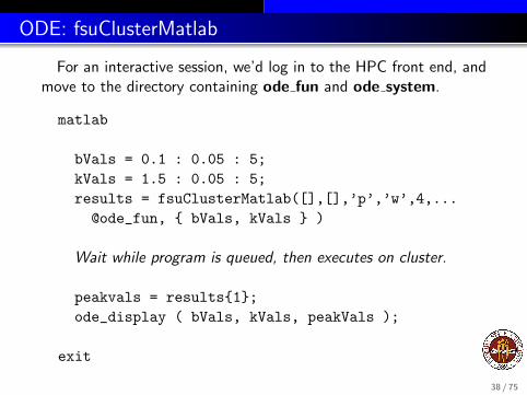
For an interactive session, we’d log in to the HPC front end, andmove to the directory containing ode fun and ode system.

matlab

bVals = 0.1 : 0.05 : 5;kVals = 1.5 : 0.05 : 5;results = fsuClusterMatlab([],[],’p’,’w’,4,...

@ode_fun, { bVals, kVals } )

Wait while program is queued, then executes on cluster.

peakvals = results{1};ode_display ( bVals, kVals, peakVals );

exit

38 / 75

ODE: fsuClusterMatlab with NOWAIT option

But you don’t have to wait. You can send your job, log out, andreturn to your directory later. The details of this are a little gory!

1 Jobs are numbered. My last job is called Job8.

2 cat Job8.state.mat prints finished if the job is complete;

3 Now start MATLAB:

matlabcd Job8load ( ’Task1.out.mat’ )peakvals = argsout{1}; <-- what we called “results”bVals = 0.1 : 0.05 : 5;kVals = 1.5 : 0.05 : 5;ode_display ( bVals, kVals, peakVals );

exit

39 / 75


Introduction





QUAD Example (SPMD)


Conclusion

40 / 75


The SPMD command is like a very simplified version of MPI.There is one client process, supervising workers who cooperate ona single program. Each worker (sometimes also called a “lab”) hasan identifier, knows how many workers there are total, and candetermine its behavior based on that ID.

each worker runs on a separate core (ideally);

each worker uses separate workspace;

a common program is used;

workers meet at synchronization points;

the client program can examine or modify data on any worker;

any two workers can communicate directly via messages.

41 / 75

SPMD: The SPMD Environment

MATLAB sets up one special worker called the client.

MATLAB sets up the requested number of workers, each with acopy of the program. Each worker “knows” it’s a worker, and hasaccess to two special functions:

numlabs(), the number of workers;

labindex(), a unique identifier between 1 and numlabs().

The empty parentheses are usually dropped, but remember, theseare functions, not variables!

If the client calls these functions, they both return the value 1!That’s because when the client is running, the workers are not.The client could determine the number of workers available by

n = matlabpool ( ’size’ )

42 / 75

SPMD: The SPMD Command

The client and the workers share a single program in which somecommands are delimited within blocks opening with spmd andclosing with end.

The client executes commands up to the first spmd block, when itpauses. The workers execute the code in the block. Once theyfinish, the client resumes execution.

The client and each worker have separate workspaces, but it ispossible for them to communicate and trade information.

The value of variables defined in the “client program” can bereferenced by the workers, but not changed.

Variables defined by the workers can be referenced or changed bythe client, but a special syntax is used to do this.

43 / 75

SPMD: How SPMD Workspaces Are Handled

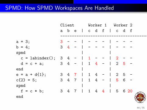
Client Worker 1 Worker 2a b e | c d f | c d f---------------------------------------------------

a = 3; 3 - - | - - - | - - -b = 4; 3 4 - | - - - | - - -spmd | |c = labindex(); 3 4 - | 1 - - | 2 - -d = c + a; 3 4 - | 1 4 - | 2 5 -

end | |e = a + d{1}; 3 4 7 | 1 4 - | 2 5 -c{2} = 5; 3 4 7 | 1 4 - | 5 6 -spmd | |f = c * b; 3 4 7 | 1 4 4 | 5 6 20

end

44 / 75

SPMD: When is Workspace Preserved?

A program can contain several spmd blocks. When execution ofone block is completed, the workers pause, but they do notdisappear and their workspace remains intact. A variable set in onespmd block will still have that value if another spmd block isencountered.

You can imagine the client and workers simply alternate execution.

In MATLAB, variables defined in a function “disappear” once thefunction is exited. The same thing is true, in the same way, for aMATLAB program that calls a function containing spmd blocks.While inside the function, worker data is preserved from one blockto another, but when the function is completed, the worker datadefined there disappears, just as the regular MATLAB data does.

45 / 75


Introduction





QUAD Example (SPMD)


Conclusion

46 / 75

QUAD: The Trapezoid Rule

Area of one trapezoid = average height * base.

47 / 75

QUAD: The Trapezoid Rule

To estimate the area under a curve using one trapezoid, we write∫ b

af (x) dx ≈ (

1

2f (a) +

1

2f (b)) ∗ (b − a)

We can improve this estimate by using n − 1 trapezoids defined byequally spaced points x1 through xn:∫ b

af (x) dx ≈ (

1

2f (x1) + f (x2) + ... + f (xn−1) +

1

2f (xn)) ∗ b − a

n − 1

If we have several workers available, then each one can get a partof the interval to work on, and compute a trapezoid estimatethere. By adding the estimates, we get an approximate to theintegral of the function over the whole interval.

48 / 75

QUAD: Use the ID to assign work

To simplify things, we’ll assume our original interval is [0,1], andwe’ll let each worker define a and b to mean the ends of itssubinterval. If we have 4 workers, then worker number 3 will beassigned [1

2 , 34 ].

To start our program, each worker figures out its interval:

fprintf ( 1, ’ Set up the integration limits:\n’ );

spmda = ( labindex - 1 ) / numlabs;b = labindex / numlabs;

end

49 / 75

QUAD: One Name Must Reference Several Values

Each worker is a program with its own workspace. It can “see” thevariables on the client, but it usually doesn’t know or care what isgoing on on the other workers.

Each worker defines a and b but stores different values there.

The client can “see” the workspace of any worker by specifying theworker index. Thus a{1} is how the client refers to the variable aon worker 1. The client can read or write this value.

MATLAB’s name for this kind of variable, indexed using curlybrackets, is a composite variable. It is very similar to a cell array.

The workers can “see” but not change the client’s variables.

50 / 75

QUAD: Dealing with Composite Variables

So in QUAD, each worker could print its own a and b:

spmda = ( labindex - 1 ) / numlabs;b = labindex / numlabs;fprintf ( 1, ’ A = %f, B = %f\n’, a, b );

end------------ or the client could print them all ------------spmda = ( labindex - 1 ) / numlabs;b = labindex / numlabs;

endfor i = 1 : 4 <-- "numlabs" wouldn’t work here!fprintf ( 1, ’ A = %f, B = %f\n’, a{i}, b{i} );

end

51 / 75

QUAD: The Solution in 4 Parts

Each worker can now carry out its trapezoid computation:

spmdx = linspace ( a, b, n );fx = f ( x ); (Assume f can handle vector input.)quad_part = ( b - a ) / ( n - 1 ) *

* ( 0.5 * fx(1) + sum(fx(2:n-1)) + 0.5 * fx(n) );fprintf ( 1, ’ Partial approx %f\n’, quad_part );

end

with result:

2 Partial approx 0.8746764 Partial approx 0.5675881 Partial approx 0.9799153 Partial approx 0.719414

52 / 75

QUAD: Combining Partial Results

Having each worker print out its piece of the answer is not theright thing to do. (Imagine if we use 100 workers!)

The client should gather the values together into a sum:

quad = sum ( quad_part{1:4} );fprintf ( 1, ’ Approximation %f\n’, quad );

with result:

Approximation 3.14159265

53 / 75

QUAD: Source Code for QUAD FUN

f u n c t i o n v a l u e = quad fun ( n )

f p r i n t f ( 1 , ’ Compute l i m i t s \n ’ ) ;spmd

a = ( l a b i n d e x − 1 ) / numlabs ;b = l a b i n d e x / numlabs ;f p r i n t f ( 1 , ’ Lab %d works on [%f ,% f ] .\ n ’ , l a b i nd e x , a , b ) ;

end

f p r i n t f ( 1 , ’ Each l a b e s t ima t e s pa r t o f the i n t e g r a l .\n ’ ) ;

spmdx = l i n s p a c e ( a , b , n ) ;f x = f ( x ) ;quad pa r t = ( b − a ) ∗ ( f x (1 ) + 2 ∗ sum ( f x ( 2 : n−1) ) + f x ( n ) ) . . .

/ 2 . 0 / ( n − 1 ) ;f p r i n t f ( 1 , ’ Approx %f\n ’ , quad pa r t ) ;

end

quad = sum ( quad pa r t {:} ) ;f p r i n t f ( 1 , ’ Approx imat ion = %f\n ’ , quad )

r e t u r nend

54 / 75

QUAD: Local Interactive Execution

SPMD programs execute locally just like PARFOR programs.


n = 10000;value = quad_fun ( n );

matlabpool close

55 / 75


Introduction





QUAD Example (SPMD)


Conclusion

56 / 75

DISTANCE: A Classic Problem

Consider the problem of determining the shortest path from afixed city to all other cities on a road map, or more generally, froma fixed node to any other node on an abstract graph whose linkshave been assigned lengths.

Suppose the network of roads is described using a one-hop distancematrix; the value ohd(i,j) records the length of the direct roadfrom city i to city j, or ∞ if no such road exists.

Our goal is, starting from the array ohd, to determine a new vectordistance, which records the length of the shortest possible routefrom the fixed node to all others.

57 / 75

DISTANCE: An Intercity Map

Recall our example map with the intercity highway distances:

58 / 75

DISTANCE: An Intercity One-Hop Distance Matrix

Here is the “one-hop distance” matrix ohd(i,j):

A B C D E F

A 0 40 15 ∞ ∞ ∞B 40 0 20 10 25 6C 15 20 0 100 ∞ ∞D ∞ 10 100 0 ∞ ∞E ∞ 25 ∞ ∞ 0 8F ∞ 6 ∞ ∞ 8 0

An entry of ∞ means no direct route between the cities.

59 / 75

DISTANCE: Dijkstra’s algorithm

Dijkstra’s algorithm for the minimal distances:

Use two arrays, connected and distance.Initialize connected to false except for A.Initialize distance to the one-hop distance from A to each city.Do N-1 iterations, to connect one more city at a time:

1 Find I, the unconnected city with minimum distance[I];

2 Connect I;

3 For each unconnected city J, see if the trip from A to I to J isshorter than the current distance[J].

The check we make in step 3 is:distance[J] = min ( distance[J], distance[I] + ohd[I][J] )

60 / 75

DISTANCE: A Sequential Code

connected(1) = 1;connected(2:n) = 0;

distance(1:n) = ohd(1,1:n);

for step = 2 : n

[ md, mv ] = find_nearest ( n, distance, connected );

connected(mv) = 1;

distance = update_distance ( nv, mv, connected, ...ohd, distance );

end61 / 75

DISTANCE: Parallelization Concerns

Although the program includes a loop, it is not a parallelizableloop! Each iteration relies on the results of the previous one.

However, let us assume we have a very large number of cities todeal with. Two operations are expensive and parallelizable:

find nearest searches for the nearest unconnected node;

update distance checks the distance of each unconnectednode to see if it can be reduced.

These operations can be parallelized by using SPMD statements inwhich each worker carries out the operation for a subset of thenodes. The client will need to be careful to properly combine theresults from these operations!

62 / 75

DISTANCE: Startup

We assign to each worker the node subset S through E.We will try to preface worker data by “my ”.

spmdnth = numlabs ( );my_s = floor ( ( ( labindex() - 1 ) * nv ) / nth ) + 1;my_e = floor ( ( labindex() * nv ) / nth );

end

63 / 75

DISTANCE: FIND NEAREST

Each worker uses find nearest to search its range of cities forthe nearest unconnected one.

But now each worker returns an answer. The answer we want is thenode that corresponds to the smallest distance returned by all theworkers, and that means the client must make this determination.

64 / 75

DISTANCE: FIND NEAREST

lab count = nth{1};

for step = 2 : nspmd

[ my_md, my_mv ] = find_nearest ( my_s, my_e, n, ...distance, connected );

endmd = Inf;mv = -1;for i = 1 : lab_countif ( my_md{i} < md )md = my_md{i};mv = my_mv{i};

endenddistance(mv) = md;

65 / 75

DISTANCE: UPDATE DISTANCE

We have found the nearest unconnected city.

We need to connect it.

Now that we know the minimum distance to this city, we need tocheck whether this decreases our estimated minimum distances toother cities.

66 / 75

DISTANCE: UPDATE DISTANCE

connected(mv) = 1;

spmdmy_distance = update_distance ( my_s, my_e, n, mv, ...

connected, ohd, distance );end

distance = [];for i = 1 : lab_countdistance = [ distance, my_distance{:} ];

end

end

67 / 75

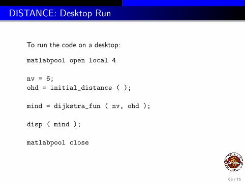
DISTANCE: Desktop Run

To run the code on a desktop:


nv = 6;ohd = initial_distance ( );

mind = dijkstra_fun ( nv, ohd );

disp ( mind );

matlabpool close

68 / 75

DISTANCE: fsuClusterMatlab

On the FSU HPC cluster, invoke fsuClusterMatlab:

nv = 6;ohd = initial_distance ( );

results = fsuClusterMatlab([],[],’m’,’w’,4,...@dijkstra_fun, { nv, ohd } );

mind = results{1};disp ( mind );

Here, the ’m’ argument indicates that this is an ”MPI-like” job,that is, it invokes the spmd command.

69 / 75

DISTANCE: Comments

This example shows SPMD workers interacting with the client.

It’s easy to divide up the work here. The difficulties come whenthe workers return their partial results, and the client mustassemble them into the desired answer.

In one case, the client must find the minimum from a smallnumber of suggested values.

In the second, the client must rebuild the distance array from theindividual pieces updated by the workers.

Workers are not allowed to modify client data. This keeps theclient data from being corrupted, at the cost of requiring the clientto manage all such changes.

70 / 75


Introduction





QUAD Example (SPMD)


Conclusion

71 / 75

Conclusion: A Parallel Version of MATLAB

Parallel MATLAB allows programmers to advance in the newworld of parallel programming.

They can benefit from many of the same new algorithms, multicorechips and multi-node clusters that define parallel computing.

When you use the parfor command, MATLAB automaticallydetermines from the form of your loop which variables are to beshared, or private, or are reduction variables; in OpenMP you mustrecognize and declare all these facts yourself.

When you use the spmd command, MATLAB takes care of all thedata transfers that an MPI programmer must carry out explicitly.

72 / 75

Conclusion: Desktop Experiments

If you are interested in parallel MATLAB, the first thing to do isget access to the Parallel Computing Toolbox on your multicoredesktop machine, so that you can do experimentation and practiceruns.

You can begin with some of the sample programs we havediscussed today.

You should then see whether the parfor or spmd approaches wouldhelp you in your own programming needs.

73 / 75

Conclusion: FSU HPC Cluster

If you are interested in serious parallel MATLAB computing, youshould consider requesting an account on the FSU HPC cluster,which offers MATLAB on up to 16 cores.

To get an account, go to www.hpc.fsu.edu and look at theinformation under Apply for an Account.

Accounts on the general access cluster are available to any FSUfaculty member, or to persons they sponsor.

74 / 75

CONCLUSION: Where is it?

MATLAB Parallel Computing Toolbox User’s Guide 5.0www.mathworks.com/access/helpdesk/help/pdf doc/distcomp/...distcomp.pdf

http://people.sc.fsu.edu/∼jburkardt/presentations/. . .fsu 2011 matlab parallel.pdf these slides;

Gaurav Sharma, Jos Martin,MATLAB: A Language for Parallel Computing,International Journal of Parallel Programming,Volume 37, Number 1, pages 3-36, February 2009.

http://people.sc.fsu.edu/∼jburkardt/m src/m src.html

quad parforode sweep parforquad spmddijkstra spmd

75 / 75

Documents

Parallel MATLAB at FSU: PARFOR and SPMDjburkardt/presentations/matlab_parallel... · MATLAB Parallel Computing Introduction PARFOR: a Parallel FOR Loop QUAD Example (PARFOR) ODE Example