Parallel Programming - National Tsing Hua Universityychung/slides/para_programming/slides1.pdf · Parallel Programming Techniques and Applications using Networked Workstations and

Page 1

Slides for Parallel Programming: Techniques and Applications using Networked Workstations and Parallel ComputersBarry Wilkinson and Michael Allen Prentice Hall, 1999. All rights reserved.

Parallel ProgrammingTechniques and Applications using Networked

Workstations and Parallel Computers

Slides

Barry Wilkinson and Michael Allen Prentice Hall, 1999

Page

Chapter 1 Parallel Computers 2

Chapter 2 Message-Passing Computing 29

Chapter 3 Embarrassingly Parallel Computations 63

Chapter 4 Partitioning and Divide-and-Conquer Strategies 78

Chapter 5 Pipelined Computations

Chapter 6 Synchronous Computations

Chapter 7 Load Balancing and Termination Detection

Chapter 8 Programming with Shared Memory

Chapter 9 Sorting Algorithms

Chapter 10 Numerical Algorithms

Chapter 11 Image Processing

Chapter 12 Searching and Optimization

Page 2


Chapter 1 Parallel Computers

The Demand for Computational Speed

Continual demand for greater computational speed from a computer system than is

currently possible. Areas requiring great computational speed include numerical

modeling and simulation of scientific and engineering problems. Computations must be

completed within a “reasonable” time period.

Grand Challenge Problems

A grand challenge problem is one that cannot be solved in a reasonable amount of time

with today’s computers. Obviously, an execution time of 10 years is always

unreasonable.

Examples: Modeling large DNA structures, global weather forecasting, modeling

motion of astronomical bodies.

Weather Forecasting

Atmosphere is modeled by dividing it into three-dimensional regions or cells. The

calculations of each cell are repeated many times to model the passage of time.

ExampleWhole global atmosphere divided into cells of size 1 mile × 1 mile × 1 mile to a height

of 10 miles (10 cells high) - about 5 × 108 cells.

Suppose each calculation requires 200 floating point operations. In one time step, 1011

floating point operations necessary.

To forecast the weather over 10 days using 10-minute intervals, a computer operating at

100 Mflops (108 floating point operations/s) would take 107 seconds or over 100 days.

To perform the calculation in 10 minutes would require a computer operating at 1.7

Tflops (1.7 × 1012 floating point operations/sec).

Page 3


Modeling Motion of Astronomical Bodies

Predicting the motion of the astronomical bodies in space. Each body is attracted to

each other body by gravitational forces. Movement of each body can be predicted by

calculating the total force experienced by the body.

If there are N bodies, N − 1 forces to calculate for each body, or approximately N2

calculations, in total. (N log2 N for an efficient approximate algorithm.) After

determining the new positions of the bodies, the calculations must be repeated.

A galaxy might have, say, 1011 stars. Even if each calculation could be done in 1µs

(10−6 seconds, an extremely optimistic figure), it would take 109 years for one iteration

using the N2 algorithm and almost a year for one iteration using the N log2 N efficient

approximate algorithm.

Figure 1.1 Astrophysical N-body simulation by Scott Linssen (undergraduate University of North Carolina at Charlotte [UNCC] student).

Page 4


Parallel Computers and Programming

Using multiple processors operating together on a single problem. Not a new idea; in

fact it is a very old idea. Gill writes in 1958:

“... There is therefore nothing new in the idea of parallel programming, but itsapplication to computers. The author cannot believe that there will be any insuperabledifficulty in extending it to computers. It is not to be expected that the necessaryprogramming techniques will be worked out overnight. Much experimenting remainsto be done. After all, the techniques that are commonly used in programming todaywere only won at the cost of considerable toil several years ago. In fact the advent ofparallel programming may do something to revive the pioneering spirit in programmingwhich seems at the present to be degenerating into a rather dull and routine occupation...”

Gill, S. (1958), “Parallel Programming,” The Computer Journal, vol. 1, April, pp. 2-10.

Notwithstanding the long history, Flynn and Rudd (1996) write that “ … leads us to onesimple conclusion: the future is parallel.” We concur.

Figure 1.2 Conventional computer having a single processor and memory.

Main memory

Processor

Instructions (to processor)Data (to or from processor)

Types of Parallel Computers

A conventional computer consists of a processor executing a program stored in a

(main) memory:

Each main memory location in the memory in all computers is located by a number

called its address. Addresses start at 0 and extend to 2n − 1 when there are n bits (binary

digits) in the address.

Page 5


Figure 1.3 Traditional shared memory multiprocessor model.

Processors

Interconnectionnetwork

Memory modulesOneaddressspace

Shared Memory Multiprocessor System

A natural way to extend the single processor model is to have multiple processors

connected to multiple memory modules, such that each processor can access any

memory module in a so-called shared memory configuration:

Programming Shared Memory Multiprocessor

Can be done in different ways:

Parallel Programming Languages

With special parallel programming constructs and statements that allow shared

variables and parallel code sections to be declared. Then the compiler is responsible for

producing the final executable code.

Threads

Threads can be used that contain regular high-level language code sequences for

individual processors. These code sequences can then access shared locations.

Page 6


Processor


Local

Computers

Messages

Figure 1.4 Message-passing multiprocessor model (multicomputer).

memory

Message-Passing Multicomputer

Complete computers connected through an interconnection network:

Programming

Still involves dividing the problem into parts that are intended to be executed

simultaneously to solve the problem

Common approach is to use message-passing library routines that are linked to

conventional sequential program(s) for message passing.

Problem divided into a number of concurrent processes.

Processes will communicate by sending messages; this will be the only way to

distribute data and results between processes.

Page 7


Processor


Shared

Computers

Messages

Figure 1.5 Shared memory multiprocessor implementation.

memory

Distributed Shared MemoryEach processor has access to the whole memory using a single memory address space.

For a processor to access a location not in its local memory, message passing must

occur to pass data from the processor to the location or from the location to the

processor, in some automated way that hides the fact that the memory is distributed.

MIMD and SIMD Classifications

In a single processor computer, a single stream of instructions is generated from the

program. The instructions operate upon a single stream of data items. Flynn (1966)

created a classification for computers and called this single processor computer a single

instruction stream-single data stream (SISD) computer.

Multiple Instruction Stream-Multiple Data Stream (MIMD)Computer

General-purpose multiprocessor system - each processor has a separate program and

one instruction stream is generated from each program for each processor. Each

instruction operates upon different data.

Both the shared memory and the message-passing multiprocessors so far described are

in the MIMD classification.

Page 8


Single Instruction Stream-Multiple Data Stream (SIMD) Computer

A specially designed computer in which a single instruction stream is from a single

program, but multiple data streams exist. The instructions from the program are

broadcast to more than one processor. Each processor executes the same instruction in

synchronism, but using different data.

Developed because there are a number of important applications that mostly operate

upon arrays of data.

Figure 1.6 MPMD structure.

Program

Processor

Data

Program

Processor

Data

InstructionsInstructions

Multiple Program Multiple Data (MPMD) Structure

Within the MIMD classification, which we are concerned with, each processor will

have its own program to execute:

Page 9


Single Program Multiple Data (SPMD) Structure

Single source program is written and each processor will execute its personal copy of

this program, although independently and not in synchronism.

The source program can be constructed so that parts of the program are executed by

certain computers and not others depending upon the identity of the computer.

P M

C

P M

C

P M

C

Figure 1.7 Static link multicomputer.

Computers

Network with direct linksbetween computers

Message-Passing MulticomputersStatic Network Message-Passing Multicomputers

Page 10


Linksto other

nodes

Switch

Processor Memory

Computer (node)

Linksto othernodes

Figure 1.8 Node with a switch for internode message transfers.

Link

Figure 1.9 A link between two nodes with separate wires in each direction.

NodeNode

Page 11


Network Criteria

Cost - indicated by number of links in network. (Ease of construction is also important.)

Bandwidth - number of bits that can be transmitted in unit time, given as bits/sec.

Network latency - time to make a message transfer through network.

Communication latency - total time to send message, including software overhead

and interface delays.

Message latency or startup time - time to send a zero-length message. Essentially the

software and hardware overhead in sending message and the actual transmission time.

Diameter - minimum number of links between two farthest nodes in the network. Only

shortest routes used. Used to determine worst case delays.

Bisection width of a network - number of links (or sometimes wires) that must be cut

to divide network into two equal parts. Can provide a lower bound for messages in a

parallel algorithm.

Figure 1.10 Ring.

Interconnection Networks

Page 12


Figure 1.11 Two-dimensional array (mesh).

LinksComputer/processor

Figure 1.12 Tree structure.

Processingelement

Root

Links

Page 13


Figure 1.13 Three-dimensional hypercube.

000 001

010 011

100

110

101

111

0000 0001

0010 0011

0100

0110

0101

0111

1000 1001

1010 1011

1100

1110

1101

1111

Figure 1.14 Four-dimensional hypercube.

Page 14


Figure 1.15 Embedding a ring onto a torus.

Ring

EmbeddingDescribes mapping nodes of one network onto another network. Example - a ring can

be embedded in a torus:

Figure 1.16 Embedding a mesh into a hypercube.

00

01

11

10

00 01 11 10yx

Nodal address1011

Page 15


Dilation - used to indicate the quality of the embedding.

The dilation is the maximum number of links in the “embedding” network

corresponding to one link in the “embedded” network.

Perfect embeddings, such as a line/ring into mesh/torus or a mesh onto a hypercube,

have a dilation of 1.

Sometimes it may not be possible to obtain a dilation of 1.

Example, mapping a tree onto a mesh or hypercube does not result in a dilation of 1

except for very small trees of height 2:

Figure 1.17 Embedding a tree into a mesh.

Root

A

A

A

A

A

A

Page 16


Communication Methods

Circuit Switching

Involves establishing path and maintaining all links in path for message to pass,

uninterrupted, from source to destination. All links are reserved for the transfer until

message transfer is complete.

Simple telephone system (not using advanced digital techniques) is an example of a

circuit-switched system. Once a telephone connection is made, the connection is

maintained until the completion of the telephone call.

Circuit switching suffers from forcing all the links in the path to be reserved for the

complete transfer. None of links can be used for other messages until the transfer is

completed.

Packet Switching,

Message divided into “packets” of information, each of which includes source and

destination addresses for routing packet through interconnection network. Maximum

size for the packet, say 1000 data bytes. If message is larger than this, more than one

packet must be sent through network. Buffers provided inside nodes to hold packets

before they are transferred onward to the next node. This form called store-and-

forward packet switching.

Mail system is an example of a packet-switched system. Letters moved from mailbox

to post office and handled at intermediate sites before being delivered to destination.

Enables links to be used by other packets once the current packet has been forwarded.

Incurs a significant latency since packets must first be stored in buffers within each

node, whether or not an outgoing link is available.

Page 17


Virtual Cut-Through,

Can eliminated storage latency. If the outgoing link is available, the message is

immediately passed forward without being stored in the nodal buffer; i.e., it is “cut

through.” If complete path were available, the message would pass immediately

through to the destination. However, if path is blocked, storage is needed for the

complete message/packet being received.

HeadPacket

Request/Acknowledge

signal(s)

Figure 1.18 Distribution of flits.

Flit buffer

Movement

Wormhole routing

Message divided into smaller units called flits (flow control digits). Only head ofmessage initially transmitted from source node to next node when connecting linkavailable. Subsequent flits of message transmitted when links become available. Flitscan become distributed through network.

Page 18


Data

R/A

Source Destinationprocessor processor

Figure 1.19 A signaling method between processors for wormhole routing (Ni and McKinley, 1993).

Request/acknowledge system

A way to “pull” flits along. Only requires a single wire between the sending node andreceiving node, called R/A (request/acknowledge).

R/A reset to 0 by receiving node when ready to receive flit (its flit buffer empty).R/A set to 1 by sending node when sending node is about to send flit.Sending node must wait for R/A = 0 before setting it to a 1 and sending the flit.Sending node knows data has been received when receiving node resets R/A to a 0.

Packet switching

Circuit switchingWormhole routing

Distance

Network

(number of nodes between source and destination)

latency

Figure 1.20 Network delay characteristics.

Page 19


Messages

Node 1 Node 2

Node 3Node 4

Figure 1.21 Deadlock in store-and-forward networks.

DeadlockOccurs when packets cannot be forwarded to next node because they are blocked byother packets waiting to be forwarded and these packets are blocked in a similar waysuch that none of the packets can move.

ExampleNode 1 wishes to send a message through node 2 to node 3. Node 2 wishes to send amessage through node 3 to node 4. Node 3 wishes to send a message through node 4 tonode 1. Node 4 wishes to send a message through node 1 to node 2.

Physical link

Virtual channel

Route

buffer Node Node

Figure 1.22 Multiple virtual channels mapped onto a single physical channel.

Virtual Channels

A general solution to deadlock. The physical links or channels are the actual hardware

links between nodes. Multiple virtual channels are associated with a physical channel

and time-multiplexed onto the physical channel.

Page 20


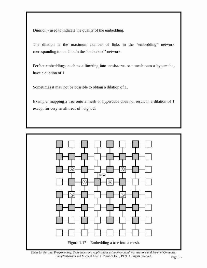
Networked Computers as a Multicomputer Platform

A cluster of workstations (COWs), or network of workstations (NOWs), offers a very

attractive alternative to expensive supercomputers and parallel computer systems for

high-performance computing. Key advantages are as follows:

• Very high performance workstations and PCs are

readily available at low cost.

• The latest processors can easily be incorporated into

the system as they become available.

• Existing software can be used or modified.

Parallel Programming Software Tools for Clusters

Parallel Virtual Machine (PVM) - developed inthe late 1980’s. Became very popular.

Message-Passing Interface (MPI) - standard was defined in 1990s.

Page 21


Workstations

Figure 1.23 Ethernet-type single wire network.

Workstation/

Ethernet

file server

Ethernet

Common communication network for workstations

Consisting of a single wire to which all the computers attach:

Figure 1.24 Ethernet frame format.

Preamble

(64 bits)

Destinationaddress(48 bits)

Sourceaddress(48 bits)

Type

(16 bits)

Data

(variable)

Frame checksequence(32 bits)

Direction

Page 22


Network

Workstation/

Workstations

Figure 1.25 Network of workstations connected via a ring.

file server

Ring Structures

Examples - token rings/FDDI networks

Workstation/file server

Workstations

Figure 1.26 Star connected network.

Point-to-point Communication

Provides the highest interconnection bandwidth. Various point-to-point configurations

can be created using hubs and switches.

Examples - High Performance Parallel Interface (HIPPI), Fast (100 MHz) and Gigabit

Ethernet, and fiber optics.

Page 23


Figure 1.27 Overlapping connectivity Ethernet.

Using separate Ethernet interfaces

Overlapping Connectivity Networks

Have characteristic that regions of connectivity are provided and regions overlap.

Several ways overlapping connectivity can be achieved. Example using Ethernet:

Speedup Factor

where ts is execution time on a single processor and tp is execution time on a

multiprocessor. S(n) gives increase in speed in using a multiprocessor. Underlying

algorithm for parallel implementation might be (and is usually) different.

Speedup factor can also be cast in terms of computational steps:

The maximum speedup is n with n processors (linear speedup).

S(n) = Execution time using one processor (single processor system)Execution time using a multiprocessor with n processors

=ts

tp

S(n) = Number of computational steps using one processorNumber of parallel computational steps with n processors

Page 24


Superlinear Speedup

where S(n) > n, may be seen on occasion, but usually this is due to using a suboptimal

sequential algorithm or some unique feature of the architecture that favors the parallel

formation.

One common reason for superlinear speedup is the extra memory in the multiprocessor

system which can hold more of the problem data at any instant, it leads to less,

relatively slow disk memory traffic. Superlinear speedup can occur in search

algorithms.

Time

Process 1

Process 2

Process 3

Process 4

Waiting to send a message

Figure 1.28 Space-time diagram of a message-passing program.

Message

Computing

Slope indicating timeto send message

Page 25


Serial section Parallelizable sections

(a) One processor

(b) Multipleprocessors

fts (1 − f)ts

ts

(1 − f)ts /n

Figure 1.29 Parallelizing sequential problem — Amdahl’s law.

tp

n processors

Maximum Speedup

Speedup factor is given by

This equation is known as Amdahl’s law

S(n) = ts n=

fts + (1 − f )ts /n 1 + (n − 1)f

Page 26


Figure 1.30 (a) Speedup against number of processors. (b) Speedup against serial fraction, f.

4

8

12

16

20

0.2 0.4 0.6 0.8 1.0Serial fraction, f

(b)

n = 256

n = 164

8

12

16

20

4 8 12 16 20

f = 20%

f = 10%

f = 5%

f = 0%

Number of processors, n

(a)

Even with infinite number of processors, maximum speedup limited to 1/f . Forexample, with only 5% of computation being serial, maximum speedup is 20,irrespective of number of processors.

Efficiency

which leads to

when E is given as a percentage.

Efficiency gives fraction of time that processors are being used on computation.

EExecution time using one processor

Execution time using a multiprocessor number of processors×------------------------------------------------------------------------------------------------------------------------------------------------------=

ts

t p n×-------------=

E = S(n) × 100%n

Page 27


Cost

The processor-time product or cost (or work) of a computation defined as

Cost = (execution time) × (total number of processors used)

The cost of a sequential computation is simply its execution time, ts. The cost of a

parallel computation is tp × n. The parallel execution time, tp, is given by ts /S(n).

Hence, the cost of a parallel computation is given by

Cost-Optimal Parallel Algorithm

One in which the cost to solve a problem on a multiprocessor is proportional to the cost

(i.e., execution time) on a single processor system.

Costtsn

S n( )-----------

ts

E---==

Scalability

Used to indicate a hardware design that allows the system to be increased in size and in

doing so to obtain increased performance - could be described as architecture or

hardware scalablity.

Scalability is also used to indicate that a parallel algorithm can accommodate increased

data items with a low and bounded increase in computational steps - could be described

as algorithmic scalablity.

Page 28


Problem Size

Intuitively, we would think of the number of data elements being processed in the

algorithm as a measure of size.

However, doubling the problem size would not necessarily double the number of

computational steps. It will depend upon the problem.

For example, adding two matrices has this effect, but multiplying matrices does not.

The number of computational steps for multiplying matrices quadruples.

Hence, scaling different problems would imply different computational requirements.

Alternative definition of problem size is to equate problem size with the number of

basic steps in the best sequential algorithm.

Gustafson’s Law

Rather than assume that the problem size is fixed, assume that the parallel executiontime is fixed. In increasing the problem size, Gustafson also makes the case that theserial section of the code does not increase as the problem size.

Scaled Speedup Factor

The scaled speedup factor becomes

called Gustafson’s law.

ExampleSuppose a serial section of 5% and 20 processors; the speedup according to the formulais 0.05 + 0.95(20) = 19.05 instead of 10.26 according to Amdahl’s law. (Note, however,the different assumptions.)

Ss n( ) s np+s p+--------------- s np+ n 1 n–( )s+= = =

Documents

Parallel Programming - National Tsing Hua Universityychung/slides/para_programming/slides1.pdf · Parallel Programming Techniques and Applications using Networked Workstations and