Parallel Solution to the Radiative Transport - KIT · PDF fileParallel Solution to the Radiative Transport László Szirmay-Kalos1, Gábor Liktor1, ... Radiance L(~x;~w)is often expressed

Eurographics Symposium on Parallel Graphics and Visualization (2009)J. Comba, K. Debattista, and D. Weiskopf (Editors)

Parallel Solution to the Radiative Transport

László Szirmay-Kalos1, Gábor Liktor1, Tamás Umenhoffer1, Balázs Tóth1, Shree Kumar2 and Glenn Lupton3

1Budapest University of Technology and Economics, Hungary2Hewlett-Packard, India, 3Hewlett-Packard, USA

AbstractThis paper presents a fast parallel method to compute the solution of the radiative transport equation in inho-mogeneous participating media. The efficiency of the method comes from different factors. First, we use a novelapproximation scheme to find a good guess for both the direct and the scattered component. This scheme is basedon the analytic solution for homogeneous media, which is modulated by the local material properties. Then, theinitial approximation is refined iteratively. The iterative refinement is executed on a face centered cubic grid, whichis decomposed to blocks according to the available simulation nodes. The implementation uses CUDA and runson a cluster of GPUs. We also show how the communication bottleneck can be avoided by not exchanging theboundary conditions in every iteration step.

1. Introduction

The multiple-scattering simulation in participating media isone of the most challenging problems in computer graph-ics, radiotherapy, PET/SPECT reconstruction, etc., whereaccurate estimates of both the direct and indirect terms areneeded not only to produce nice images, but also to recon-struct volume data from projected measurements or to makedecisions on the placement of the radiation source in thebody during radiotherapy treatment. As these applicationsrely on intensive man-machine communication, the systemis expected to respond to user actions interactively and todeliver simulation results in seconds rather than in hours,which is typical in CPU based solutions.

Such simulation should solve the radiative transportequation that expresses the change of radiance L(~x,~ω) atpoint~x and in direction ~ω:

~ω ·~∇L =dL(~x +~ωs,~ω)

ds

∣∣∣∣s=0

=

−σt(~x)L(~x,~ω)+σs(~x)∫

Ω′L(~x,~ω′)P(~ω′,~ω)dω′, (1)

where σt is the extinction coefficient describing the proba-bility of collision in a unit distance. When collision happens,the photon is either scattered or absorbed, so the extinctioncoefficient is broken down to scattering coefficient σs and

absorption coefficient σa:

σt(~x) = σa(~x)+σs(~x).

The probability of reflection given that collision happened iscalled the albedo of the material:

a =σs

σt.

If reflection happens, the probability density of the reflecteddirection is defined by phase function P(~ω′,~ω). The extentof anisotropy is usually expressed by the mean cosine of thephase function:

g =∫

Ω′(~ω′ ·~ω)P(~ω′ ·~ω)dω′.

In homogeneous media volume properties σt , σs, andP(~ω′,~ω) do not depend on position~x. In inhomogeneous me-dia these properties depend on the actual position.

In case of measured data, material properties are usuallystored in a 3D voxel grid, and are assumed to be constant orlinear between voxel centers. If the diameter of the regionrepresented by a voxel is ∆, then the total extinction is worthrepresenting by a new parameter that is called the opacityand is denoted by α:

α = 1− e−σt ∆ ≈ σt∆. (2)

Radiance L(~x,~ω) is often expressed as a sum of two terms,the direct term Ld that represents unscattered light, and the

c© The Eurographics Association 2009.

Szirmay-Kalos, Liktor, Umenhoffer, Tóth, Kumar, Lupton / Parallel Solution to the Radiative Transport

media term Lm that stands for the light component that scat-tered at least once:

L(~x,~ω) = Ld(~x,~ω)+Lm(~x,~ω).

The direct term is reduced by out-scattering:

dLdds

=−σt(~x)Ld(~x,~ω).

The media term is not only reduced by out-scattering, butalso increased by in-scattering:

dLm

ds=−σtLm +σs

∫

Ω′(Ld +Lm)P(~ω′,~ω)dω′.

Note that this equation can be re-written by considering thereflection of the direct term as a volumetric source:

dLm

ds=−σt(~x)Lm(~x,~ω)+

σs(~x)∫

Ω′Lm(~x,~ω)P(~ω′,~ω)dω′+σs(~x)Q(~x,~ω), (3)

where the source intensity is

Q(~x,~ω) =∫

Ω′Ld(~x,~ω′)P(~ω′,~ω)dω′.

The volumetric source represents the coupling between thedirect and media terms.

Although the direct term can be expressed as an integraleven in inhomogeneous media, the evaluation of this integralrequires ray marching and numerical quadrature. Having ob-tained the direct term and transformed it to the volumetricsource, the media term needs to be computed.

Cerezo et al. [CPP∗05] classified algorithms solving thetransport equation as analytic, stochastic, and iterative.

Analytic techniques rely on simplifying assumptions,such as that the volume is homogeneous, and usuallyconsider only the single scattering case [Bli82, SRNN05].Jensen et al. [JMLH01] attacked the subsurface light trans-port by assuming that the space is partitioned into two halfspaces with homogeneous material and developed the dipolemodel. Narasimhan and Nayar [NN03] proposed a multiplescattering model for optically thick homogeneous media andisotropic light source.

Stochastic methods apply Monte Carlo integration tosolve the transport problem [KH84, JC98]. These methodsare the most accurate but are far too slow in interactive ap-plications.

Iterative techniques need to represent the current radianceestimate that is refined in each step [DMK00]. The radi-ance function is specified either by finite-elements, using,for example, the zonal method [RT87], spherical harmon-ics [KH84], radial basis functions [ZRL∗08], metaballs, etc.or exploiting the particle system representation [SKSU05].

Stam [Sta95] introduced diffusion theory to compute en-ergy transport. Here the angular dependence of the radianceis approximated by a two-term expansion:

L(~x,~ω)≈ L(~x,~ω) =1

4πφ(~x)+

34π

~E(~x) ·~ω.

By enforcing the equality of the directional integrals of Land L, we get the following equation for fluence φ(~x):

φ(~x) =∫

Ω

L(~x,~ω)dω.

Requiring∫Ω

L(~x,~ω)~ω dω =∫Ω

L(~x,~ω)~ω dω, we obtain vector

irradiance ~E(~x) as

~E(~x) =∫

Ω

L(~x,~ω)~ωdω.

Substituting this two-term expansion into the radiative trans-port equation and averaging it for all directions, we obtainthe following diffusion equations:

~∇φ(~x) =−3σ′t~E(~x), ~∇·~E(~x) =−σaφ(~x). (4)

where σ′t = σt −σsg is the reduced extinction coefficient.

In [Sta95] the diffusion equation is solved by either amulti-grid scheme or a finite-element blob method. Geist etal. [GRWS04] computed multiple scattering as a diffusionprocess, using a lattice-Boltzmann solution method.

In order to speed up the solutions to interactive rates, thetransport problem is often simplified and the solution is im-plemented on the GPU. The translucent rendering approach[KPHE02] involves multiple scattering simulation, but con-siders only multiple approximate forward scattering and sin-gle backward scattering. This method aims at nice imagesinstead of physical accuracy. Physically based global illumi-nation methods, like the photon map, have also been usedto solve the multiple scattering problem [QXFN07]. To im-prove speed, light paths were sampled on a finite grid.

The high computational burden of multiple scatteringsimulation has been attacked by parallel methods both insurface [ACD08] and volume rendering [SMW∗04]. Parallelvolume rendering methods considered the visualization ofvery large datasets, while interactive multiple scattering sim-ulation has not been in focus yet. Stochastic methods scalewell on parallel systems, so they would be primary candi-dates for parallel machines, but their convergence rate is stilltoo slow. Iterative techniques, on the other hand, convergefaster but require data exchanges between the nodes, whichmakes scalability sub-linear.

This paper presents a fast parallel solution for the radiativetransport equation (Figure 1). We have taken the iterationapproach because of its better convergence. This posed chal-lenges for the parallel implementation because we shouldattack the sub-linear scalability and the communication bot-tleneck. Our approach is based on two observations. Iteration



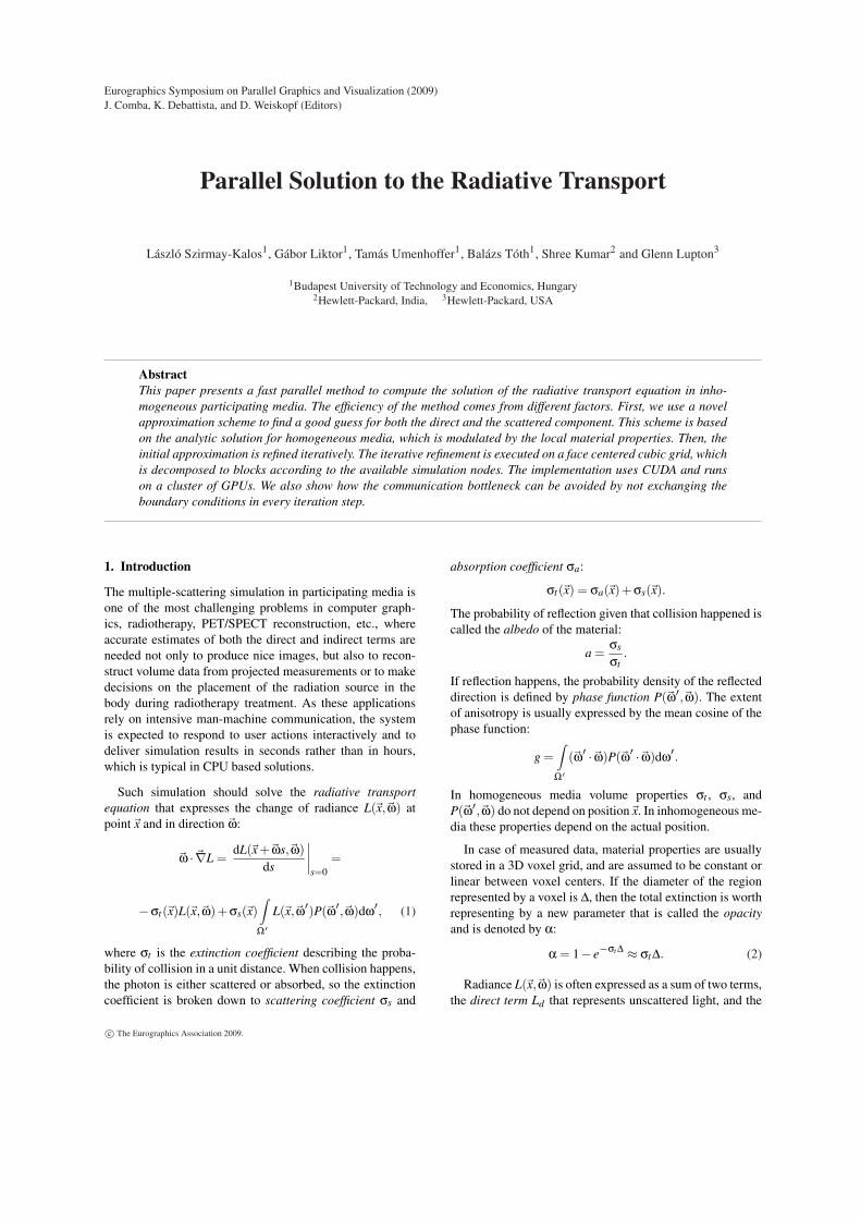
Figure 1: The outline of the algorithm. 1: The volume is de-fined on a grid. 2: An illumination network is establishedbetween the grid points. 3: Single scattering and estimatedmultiple scattering are distributed from each light source. 4:The final results are obtained by iteration which corrects theerrors of the estimation. 5: The image is rendered by stan-dard alpha blending.

is slow because it requires many “warming up” steps to dis-tribute the power of sources to far regions. Thus, if we canfind an easy way to approximate the solution, then iterationshould only refine the initial approximation, which could bedone in significantly fewer steps. On the other hand, iterationrequires the exchange of data from all computing nodes ineach step, which leads to a communication bottleneck. Wepropose an iteration scheme when the data are exchangedless frequently. This slows down the convergence of the iter-ation, so computing nodes should work longer, but reducesthe communication load.

We shall assume that the primary source of illumination isa single point light source in the origin of our coordinate sys-tem. More complex light sources can be modeled by transla-tion and superposition. We use a simple and fast technique toinitially distribute the light in the medium. The distributionis governed by the diffusion theory, where the single pass ap-proximate solution is made possible by assumptions that themedium is locally homogeneous and spherically symmetric.The solution is approximate but can be obtained at the samecost as the direct term. Having obtained the initial approxi-mation, the final solution is computed by iteration on a GPUcluster.

This paper is organized as follows. Section 2 explains theiteration solution, the importance of having a good initial ap-proximation, and the challenges of parallel execution. Sec-tion 3 discusses the computation of the direct term. Section4 presents the initial estimation of the radiance. Section 5

deals with the iterative refinement. Section 6 presents ourdistributed implementation and Section 7 summarizes the re-sults.

2. Iteration solution of the radiative transport equation

The transport equation is an integro-differential equation. In-tegrating both sides, the equation can be turned to an integralequation of the following form:

L = T L +Qe

where T is a linear integral operator and Qe is the sourceterm provided by the boundary conditions. Applying finite-element techniques, the continuous radiance function is rep-resented by finite data, which turns the integrated transportequation to a system of linear equations:

L = T ·L+Qe,

where vector L is the radiance of the sample locations anddirections, Qe is the vector of source terms and boundaryconditions, and T is the transport matrix.

Iteration obtains the solution as the limiting value of thefollowing iteration sequence

Ln = T ·Ln−1 +Qe

so if this scheme is convergent, then the solution can beobtained by starting with an arbitrary radiance distributionL0 and iteratively repeating operator T. The convergence isguaranteed if T is a contraction, i.e. for the norm of this ma-trix, we have

‖T ·L‖< λ‖L‖, λ < 1,

which is the case if the albedo is less than 1.

The error at a particular step n can be found by subtractingthe solution L from the iteration scheme, and applying thedefinition of the contraction iteratively:

‖Ln−L‖= ‖T ·(Ln−1−L)‖< λ‖Ln−1−L‖< λn‖L0−L‖.Note that the error is proportional to the norm of the differ-ence of the initial guess L0 and the final solution L. Thus,having a good initial guess that is not far from the solution,the error after n iteration steps can be significantly reduced.

2.1. Iteration on parallel machines

In order to execute the iteration on a parallel machine, theradiance vector Ln is broken to parts and each computingnode is responsible for the update of its own part. However,the new value of a part also depends on other parts, whichwould necessitate state exchanges between the nodes in ev-ery iteration. This would quickly make the communicationthe bottleneck of the parallel computation.

This problem can be attacked by not exchanging the cur-rent state in every iteration cycle. Suppose, for example, that



we exchange data just in every second iteration cycle. Whenthe data is exchanged before executing the matrix-vectormultiplication, the iteration looks like the original formula:

Ln = T ·Ln−1 +Qe.

However, when the data is not exchanged, a part of the ma-trix is multiplied by the radiance estimate of the older iter-ation. Let us denote the matrix by T∗ that is similar to Twhere the own part is multiplied and zero elsewhere. Withthis notation, the cycle without previous data exchange is:

Ln = T∗ ·Ln−1 +(T−T∗) ·Ln−2 +Qe.

Putting the two equations together, the execution of an iter-ation without state changes and then an iteration with statechanges would result in:

Ln = T2 ·Ln−2 +T ·Qe +Qe +T ·(T−T∗) ·(Ln−3−Ln−2).

Note that if this scheme is convergent, then Ln, Ln−2, andLn−3 should converge to the same vector L, thus the limitingvalue satisfies the following equation:

L = T2 ·L+T ·Qe +Qe.

This equation is equivalent to the original equation, whichcan be proven if the right side’s L is substituted by the com-plete right side:

L = T ·L+Qe = T · (T ·L+Qe)+Qe.

The price of not exchanging the data in every iteration step isthe additional error term T · (T−T∗) · (Ln−3−Ln−2). Thiserror term converges to zero, but slows down the iterationprocess especially at the beginning of the iteration.

Using the same argument, we can prove a similar state-ment for cases when the data is exchanged just in everythird, fourth, etc. cycles. The number of iterations done bythe nodes between data exchanges should be specified byfinding an optimal compromise, which depends on the rela-tive computation and communications speeds.

3. Distribution of the direct term

The direct term is reduced by out-scattering. As the sourceis in the origin, the direct term is non-zero only for the di-rection from the origin to the considered point. Let us con-sider a point at distance r on a beam started at the sourceand having solid angle ∆Ω, and step on this beam by dr. Asa photon collides with the medium with probability σt(r)drduring the step, the radiant intensity (i.e. the power per solidangle) Φ(r) at distance r satisfies the following equation

Φ(r+dr) = Φ(r)−σt(r)drΦ(r) =⇒ dΦ(r)dr

=−σt(r)Φ(r).(5)

If the radiant intensity is Φ0 at the source, then the solutionof this equation is

Φ(r) = Φ0e−∫ r

0 σt (s)ds.

The radiance is the power per differential solid angle anddifferential area. In our beam the power is the product ofradiant intensity Φ(r) and solid angle ∆Ω. On the other hand,the solid angle in which the source is visible equals to zero,which introduces a Dirac delta in the radiance formula. Thearea at distance r grows as ∆A = ∆Ωr2. Thus, the radianceof the direct term is

Ld(~x,~ω) =Φ(r)∆Ω

∆Ωr2 δ(~ω−~ω~x) =Φ(r)

r2 δ(~ω−~ω~x), (6)

where r = |~x| is the distance and ~ω~x =~x/|~x| is the directionof the point from the source.

4. Initial distribution of the estimated radiance

Let us consider just a single beam starting at the origin wherethe point source is. When a beam is processed, we shall as-sume that other beams face to the same material characteris-tics, i.e. we assume that the scene is spherically symmetric.Consequently, the solution should also have spherical sym-metry.

In case of spherical symmetry, the radiance of the in-spected beam at point ~x and in direction ~ω may dependjust on distance r = |~x| from the origin and on angle θ be-tween direction ~ω and the direction of point ~x. This allowsparametrization L(r,θ) instead of L(~x,~ω). The fluence de-pends just on distance r and vector irradiance ~E(~x) has thedirection of the given point, that is ~E(~x) = E(r)~ω~x.

Expressing the divergence operator in spherical coordi-nates, we get:

~∇·~E(~x) = ~∇· (E(r)~ω~x) =1r2

∂(r2E(r))∂r

.

Thus, the scalar versions of the diffusion equations are:

dφ(r)dr

=−3σ′t E(r),1r2

d(r2E(r))dr

=−σaφ(r). (7)

For homogeneous infinite material, the differential equa-tion can be solved analytically:

φh0(r) =

3σ′t Φ0r

e−σer, Eh1 (r) =

Φ0r2 e−σer (σer +1) . (8)

where σe =√

3σaσ′t is the effective transport coefficient.

One option for the initial radiance estimation would bethe application of the homogeneous solution assuming thatthe volume everywhere has similar material properties ob-tained as the average of the real values. However, this ap-proach would provide poor estimates in regions having verydifferent scattering parameters, that is in strongly inhomo-geneous materials. Thus, we use the homogeneous solutiononly in the neighborhood of the source and farther away dif-ferential equation 7 is iterated. The volume is processed byray marching initiated at the source. The radiance of theserays forming a bundle is initialized with the homogeneoussolution.



As ray marching proceeds taking steps ∆ increasing dis-tance r, material properties σt , σs, and g are fetched at thesample location, and state variables φ(r), and E(r) are up-dated according to the numerical quadrature solving equa-tion 7, resulting in the following iteration formulae:

φ(r +∆) = φ(r)−3σ′t E(r)∆,

E(r +∆) =r2

(r +∆)2 (E(r)−σaφ(r)∆) . (9)

5. Refinement of the initial solution by iteration

At the end of the approximate radiance distribution we havegood estimates for the direct term Ld and volumetric source

Q(~x,~ω) =∫

Ω′Ld(~x,~ω′)P(~ω′,~ω)dω′ = Φ(r)

r2 P(~ω~x,~ω),

and probably less accurate estimates for the total radiance

L(~x,~ω)≈ 14π

φ(~x)+3

4π~E(~x) ·~ω.

Thus, we can accept direct term Ld , but the media termLm = L− Ld needs further refinement. We use an iterationscheme to make the media term more accurate, which isbased on equation 3, but considers only the voxel centers.The incoming medium radiance arriving at voxel p fromdirection ~ω is denoted by I(p)

m (~ω). Similarly, the outgoingmedium radiance is denoted by L(p)

m (~ω). Using these nota-tions, the discretized version of equation 3 at voxel p is:

L(p)m (~ω) = (1−α(p))I(p)

m (~ω)+

α(p)a(p)∫

Ω′I(p)m (~ω′)P(p)(~ω′,~ω)dω′+α(p)a(p)Q(p)(~ω)

(10)since σt∆≈ α and σs∆≈ αa.

The incoming radiance of a voxel is equal to the outgoingradiance of another voxel that is the neighbor in the givendirection, or it is set explicitly by the boundary conditions.Since in the discretized model a voxel has just finite numberof neighbors, the in-scattering integral can also be replacedby a finite sum:∫

Ω′I(p)(~ω′)P(p)(~ω′,~ω)dω′ ≈ 4π

D

D

∑d=1

I(p)(~ω′d)P(p)(~ω′d ,~ω).

where D is the number of neighbors, which are in direc-tions ~ω′1, . . . ,~ω

′D with respect to the given voxel. The num-

ber of neighbors depends on the structure of the grid. In aconventional Cartesian Cubic grid, a grid point has 6 neigh-bors. In a so called Body Centered Cubic grid [Cse05] avoxel has 8 neighboring voxels that share a face, which stillseems to be too small to approximate a directional integral.Thus, it is better to use a Face Centered Cubic grid (FCCgrid) [QXFN07], where each voxel has D = 12 neighbors(Figure 2).

Figure 2: Structure of the Face Centered Cubic Grid. Gridpoints are the voxel corners, voxel centers, and the centersof the voxel faces. Here every grid point has 12 neighbors,all at the same distance.

Note that unknown radiance values appear both on the leftand the right sides of the discretized transport equation. Ifwe have an estimate of radiance values (and consequently,of incoming radiance values), then these values can be in-serted into the formula of the right side and a new estimateof the radiance can be provided. Iteration keeps repeatingthis step. If the process is convergent, then in the limitingcase the formula would not alter the radiance values, whichare therefore the roots of the equation.

6. Implementation

The system has been implemented on a 5 node HP ScalableVisualization Array (SVA), where each node is equippedwith an NVIDIA GeForce 8800 GTX GPU, programmed un-der CUDA. The nodes are interconnected by Infiniband.

In order to execute ray marching parallely for all rays dur-ing initial radiance distribution, the volume is resampled toa new grid that is parameterized with spherical coordinates.A voxel of the new grid with (u,v,w) coordinates representsfluence φ and vector irradiance E of point

~x = R(wcosψsinθ,wsinψsinθ,wcosθ),

where ψ = 2πu, θ = arccos(1−2v),

and R is the radius of the volume. Note that this parametriza-tion provides uniform sampling in the directional domain. A(u,v) pair encodes a ray, while w encodes the distance fromthe origin. This texture is processed w-layer by w-layer, i.e.stepping the radius r simultaneously for all rays. In a singlestep the GPU updates the fluence and the vector irradianceaccording to equation 9.

The initial radiance distribution is not parallelized, but wetrace all rays in all nodes. However, as we terminate raysleaving the subvolume associated with a node, it can alsobenefit from the addition of more nodes. Iteration, visual-



ization, and image compositing are executed in a distributedway.

Figure 3: Decomposition of the volume to subvolumes

The tasks are distributed by subdividing the volume alongone axis and each node is responsible for both the radiativetransport simulation and the rendering of its associated sub-volume (Figure 3). The images rendered by the nodes arecomposited by the ParaComp library [Par07].

During iterational refinement separate kernels are exe-cuted on the GPU for each computational step. The radi-ance distribution for one wavelength in the FCC grid is rep-resented with 12 floating point arrays — one for each dis-crete direction in the grid. The FCC sites can be mappedinto a standard 3D array by using proper indexing, whereeach value means the outgoing radiance from a given gridsite in one direction. The volumetric source values remainconstant during the iteration, so we store them in separate3D textures. The iteration kernel updates the state of the gridby reading the emissions and the incoming radiances fromthe neighboring grid sites. The output of an iteration step isthe input of the following one, so we copy the results backto the input textures after each kernel execution. In order toimprove performance, we introduced a sensitivity constantwhich is a lower bound to the sum of the incoming radiancesfor each point. We evaluate the iteration formula only wherethe radiance value is greater than this constant. This methodis efficient if there are larger parts of the volume without sig-nificant irradiance.

In addition to executing the iteration in the individualsubvolumes, we need to implement the radiance transportbetween the neighboring volume parts. The simulation ar-eas overlap so that the radiance values can be seamlesslypassed from one subvolume to the other. MPI communica-tion between the nodes is used to exchange the solutions atthe boundary layers. It is important to notice that each nodeneeds to pass only 4 arrays to its appropriate neighbor as theFCC grid has 4 outgoing and 4 incoming directions for eachaxis-aligned boundaries.

7. Results

First, we have examined the effect of the initial radiance ap-proximation. Figure 4 shows the error curves of the itera-tion obtained when the radiance is initialized by the directterm only and when the media term approximation is alsoused. Note that the application of the media term approxima-tion halved the number of iteration steps required to obtain agiven accuracy.

0

10

20

30

40

50

60

70

80

90

100

10 20 30 40 50 60 70 80 90 100

tota

l err

or (

%)

iterations

Direct term onlyMedia term estimation

Figure 4: Error curves of the iteration when the radianceis initialized to the single-scattering term and when the ra-diance is initialized to the media term approximation. Notethat in the latter case, roughly only 50% of the iteration stepsare needed to obtain the same accuracy.

The evolution of the iteration can also be followed in Fig-ures 5 and 6. Note that if we initialize the iteration with thedirect term, we need about 100 iteration steps to eliminateany further visual change in the image (the error goes below2%). However, when the radiance is initialized to the ap-proximated media term, we obtain the same result executingonly 60 iterations.

Finally, we tested the scalability of our parallel implemen-tation. The volume is decomposed to 4 blocks along axis z(Figure 3), and the transfer of each block is computed ona separate node equipped with its own GPU. Table 1 sum-marizes the time data measured when a classical iterationscheme is executed that exchanges the boundary layers of theblocks in each iteration step, and when they are exchangedjust after every fifth iteration step. We can observe that thevisualization scales well with the introduction of new nodesbut iteration time improves just moderately when bound-ary conditions are exchanged in each iteration step, becauseof the communication bottleneck. This bottleneck can beeliminated by exchanging the boundary conditions less fre-quently, which slightly reduces the speed of convergence,so we trade communication overhead for GPU computationpower. We observed that the error caused by exchanging theboundary conditions just after every fifth iteration cycle can



direct term direct term direct term+1 iteration +25 iterations +100 iterations

density only media term estimation media term estimation+60 iterations

Figure 5: Evolution of the iteration when the radiance is initialized to the direct term and to the estimated media term, respec-tively. The radiance is color coded to emphasize the differences and is superimposed on the density field.

be compensated by about 5% more cycles, which is a goodtradeoff. Note that when we exchanged the boundary condi-tions just after every fifth iteration cycle, the iteration speedscaled well with the introduction of newer nodes.

8. Conclusions

This paper proposed an effective method to solve the radia-tive transport equation in heterogeneous participating mediaon a cluster of GPUs. The transport equation is solved onan FCC grid by iteration. The iterative algorithm has beensignificantly improved by finding a good initial guess forthe radiance and modifying the parallel implementation toreduce the frequency of data exchanges. Without these, thevery high performance of GPUs would make the communi-cation become the bottleneck. This concept of iterating moreon the nodes without exchanges gives us a versatile tool toaddress the scalability issue. We have tested the approachon a cluster of GPUs, but it is equally applicable to multiple

GPU cards inserted in the same desktop since they also sharethe problem of the communication bottleneck.

Acknowledgement

This work has been supported by the National Office for Re-search and Technology, Hewlett-Packard, OTKA K-719922(Hungary), and by the Terratomo project.

References[ACD08] AGGARWAL V., CHALMERS A., DEBATTISTA K.:

High-Fidelity Rendering of Animations on the Grid: A CaseStudy. Favre J. M., Ma K.-L., (Eds.), Eurographics Association,pp. 41–48.

[Bli82] BLINN J. F.: Light reflection functions for simulationof clouds and dusty surfaces. In SIGGRAPH ’82 Proceedings(1982), pp. 21–29.

[CPP∗05] CEREZO E., PÉREZ F., PUEYO X., SERON F. J., SIL-LION F. X.: A survey on participating media rendering tech-niques. The Visual Computer 21, 5 (2005), 303–328.



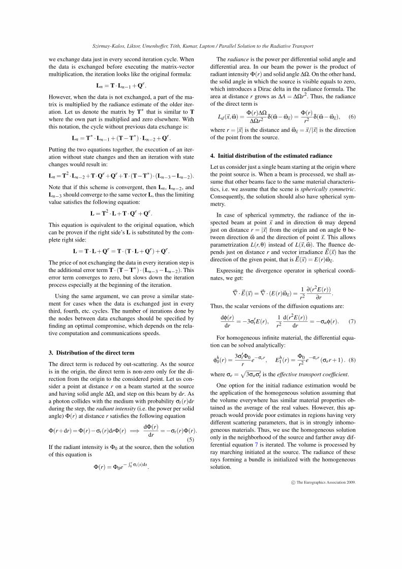
direct term direct term direct term media term converged result+1 iteration +25 iterations approximation

Figure 6: Evolution of the iteration when the radiance is initialized to the direct term and to the estimated media term, respec-tively. The radiance is color coded to emphasize the differences and is superimposed on the density field.

No Freq Initial Iteration Visual Total2 1 27 ms 19 + 23 ms 35 ms 2.6 s3 1 19 ms 12 + 25 ms 30 ms 2.2 s4 1 17 ms 8 + 29 ms 25 ms 2.1 s2 1/5 27 ms 19 + 10 ms 35 ms 1.8 s3 1/5 19 ms 12 + 10 ms 30 ms 1.4 s4 1/5 17 ms 8 + 11 ms 25 ms 1.1 s

Table 1: Performance figures with respect to the number ofnodes (“No”) and the frequency of boundary conditions ex-changes (“Freq”). The volume is a 128×128×64 resolutiongrid. The resolution of the screen is 600×600. “Initial” timeis needed by the initial radiance distribution, “Iteration” isthe sum of the time of a single iteration cycle and the time re-quired by the exchanges of the boundary conditions and tex-ture ping-pong after the iteration cycle, “Visual” is neededby the final ray casting and compositing the partial images,and “Total” is the total simulation/rendering time needed toreduce the error below 2% (60 iterations if boundary condi-tions are exchanged after each iteration and 63 iterations ifboundary conditions are exchanged after every 5 iterations).

[Cse05] CSÉBFALVI B.: Prefiltered Gaussian reconstruction forhigh-quality rendering of volumetric data sampled on a body-centered cubic grid. In VIS ’05: Visualization, 2005 (2005), IEEEComputer Society, pp. 311–318.

[DMK00] DACHILLE F., MUELLER K., KAUFMAN A.: Volu-metric global illumination and reconstruction via energy back-projection. In Symposium on Volume Rendering (2000).

[GRWS04] GEIST R., RASCHE K., WESTALL J., SCHALKOFFR.: Lattice-boltzmann lighting. In Eurographics Symposium onRendering (2004).

[JC98] JENSEN H. W., CHRISTENSEN P. H.: Efficient simulationof light transport in scenes with participating media using photonmaps. SIGGRAPH ’98 Proceedings (1998), 311–320.

[JMLH01] JENSEN H. W., MARSCHNER S., LEVOY M., HAN-

RAHAN P.: A practical model for subsurface light transport. SIG-GRAPH 2001 Proceedings (2001).

[KH84] KAJIYA J., HERZEN B. V.: Ray tracing volume densities.In SIGGRAPH ’84 Proceedings (1984), pp. 165–174.

[KPHE02] KNISS J., PREMOZE S., HANSEN C., EBERT D.: In-teractive translucent volume rendering and procedural modeling.In VIS ’02: Proceedings of the conference on Visualization ’02(2002), IEEE Computer Society, pp. 109–116.

[NN03] NARASIMHAN S. G., NAYAR S. K.: Shedding light onthe weather. In CVPR 03 (2003), pp. 665–672.

[Par07] PARACOMP: HP Scalable Visualization Array Version2.1. Tech. rep., HP, 2007. http://docs.hp.com/en/A-SVAPC-2C/A-SVAPC-2C.pdf.

[QXFN07] QIU F., XU F., FAN Z., NEOPHYTOS N.: Lattice-based volumetric global illumination. IEEE Transactions on Vi-sualization and Computer Graphics 13, 6 (2007), 1576–1583.Fellow-Arie Kaufman and Senior Member-Klaus Mueller.

[RT87] RUSHMEIER H. E., TORRANCE K. E.: The zonal methodfor calculating light intensities in the presence of a participatingmedium. In SIGGRAPH 87 (1987), pp. 293–302.

[SKSU05] SZIRMAY-KALOS L., SBERT M., UMENHOFFER T.:Real-time multiple scattering in participating media with illu-mination networks. In Eurographics Symposium on Rendering(2005), pp. 277–282.

[SMW∗04] STRENGERT M., MAGALLÓN M., WEISKOPF D.,GUTHE S., ERTL T.: Hierarchical Visualization and Compres-sion of Large Volume Datasets Using GPU Clusters . Bartz D.,Raffin B., Shen H.-W., (Eds.), Eurographics Association, pp. 41–48.

[SRNN05] SUN B., RAMAMOORTHI R., NARASIMHAN S. G.,NAYAR S. K.: A practical analytic single scattering model forreal time rendering. ACM Trans. Graph. 24, 3 (2005), 1040–1049.

[Sta95] STAM J.: Multiple scattering as a diffusion process. InEurographics Rendering Workshop (1995), pp. 41–50.

[ZRL∗08] ZHOU K., REN Z., LIN S., BAO H., GUO B., SHUMH.-Y.: Real-time smoke rendering using compensated raymarching. ACM Trans. Graph. 27, 3 (2008), 36.


Documents

Parallel Solution to the Radiative Transport - KIT · PDF fileParallel Solution to the Radiative Transport László Szirmay-Kalos1, Gábor Liktor1, ... Radiance L(~x;~w)is often expressed