Parallel solver for the three-dimensional Cartesian-grid-based time-dependent Schrödingerequation and its applications in laser-H2

+ interaction studies

Y.-M. Lee,1 J.-S. Wu,1,* T.-F. Jiang,2 and Y.-S. Chen3

1Department of Mechanical Engineering, National Chiao Tung University, 1001 Ta-Hsueh Road, Hsinchu 30050, Taiwan2Institute of Physics, National Chiao Tung University, 1001 Ta-Hsueh Road, Hsinchu 30050, Taiwan

3National Space Organization, National Applied Research Laboratories, Hsinchu 30078, Taiwan�Received 19 September 2007; revised manuscript received 26 October 2007; published 31 January 2008�

A parallelized three-dimensional Cartesian-grid-based time-dependent Schrödinger equation �TDSE� solverfor molecules with a single electron, assuming the motion of the nucleus is frozen, is presented in this paper.An explicit stagger-time algorithm is employed for time integration of the TDSE, in which the real andimaginary parts of the wave function are defined at alternate times, while a cell-centered finite-volume methodis utilized for spatial discretization of the TDSE on Cartesian grids. The TDSE solver is then parallelized usingthe domain decomposition method on distributed memory machines by applying a multilevel graph-partitioning technique. The solver is validated using a H2

+ molecule system, both by observing the totalelectron probability and total energy conservation without laser interaction, and by comparing the ionizationrates with previous two-dimensional axisymmetric simulation results with an aligned incident laser pulse. Theparallel efficiency of this TDSE solver is presented and discussed; the parallel efficiency can be as high as 75%using 128 processors. Finally, examples of the temporal evolution of the probability distribution of laserincidence onto a H2

+ molecule at inter-nuclear distance of 9 a.u. ��=0° and 90°� and the spectral intensities ofharmonic generation at internuclear distance of 2 a.u. ��=0°, 30°, 60°, and 90°� are presented to demonstratethe powerful capability of the current TDSE solver. Future possible extensions of the present method are alsooutlined at the end of this paper.

DOI: 10.1103/PhysRevA.77.013414 PACS number�s�: 32.80.Rm, 33.80.Rv, 31.70.Hq

I. INTRODUCTION

The hydrogen molecular ion H2+ is the simplest molecule.

It is usually used as a prototype in molecular physics, likethe hydrogen atom in atomic physics. The quantum dynam-ics of H2

+ and other small molecules under interaction with astrong laser pulse has been a subject of continuous interestfor more than two decades. Interesting phenomena such asbond softening, bond hardening, above-threshold dissocia-tion, and Coulomb explosion have been studied �1�. In par-ticular, a recent experiment clearly showed that the ioniza-tion rates of H2

+ at some characteristic bond lengths aregreatly enhanced by a laser pulse of �1014 W /cm2 and du-ration of several hundreds of femtoseconds. When the mol-ecule is ionized, the two positively charged bare ions repeleach other with strong Coulomb repulsion due to the smallseparation between them. Suddenly the two ions fly apartrapidly �2�. This dramatic phenomenon has been named ei-ther Coulomb explosion or charge-resonance-enhanced ion-ization.

From the computational viewpoint, the H2+ quantum sys-

tem is not simple at all. The time evolution of H2+ under a

laser field in general has nine degrees of freedom in spaceplus the time variable. This kind of time-dependentSchrödinger equation �TDSE� is unlikely to be solved evenusing the most advanced numerical schemes and computers.The calculations are often simplified with the Born-Oppenheimer approximation �BOA� where the nuclei are

fixed during the interaction with light, because the motionsof nuclei are much slower than those of electrons. It isknown that the BOA is applicable when the optical period issmaller than the vibrational period.

H2+ has two fixed nuclei and a fast-moving electron. With

a linearly polarized electric field along the molecular axis,the system is cylindrically symmetric in spatial coordinatesin addition to the time variable. The time-dependent two-dimensional TDSE has often been used because it is compu-tationally less demanding �e.g., �3–7��. However, it is stillvery difficult �or impossible� to align the molecule to beperfectly oriented with the laser field experimentally, andalso the laser field may not be linearly polarized, whichmakes the time-dependent three-dimensional �3D� computa-tion of the TDSE very desirable. Unfortunately, this kind ofcalculation is still very limited and still in its infancy due tothe very high computational cost, even with the rapid ad-vancement of computer technology. Until very recently, therehave been three types of numerical method used in solvingthe 3D TDSE for the study of laser-molecule interaction. �1�First the 3D TDSE was transformed from Cartesian coordi-nates into spheroidal coordinates and then the transformedequation was solved using the basis expansion techniquewith high-order Taylor’s series expansion for time propaga-tion ��8,9�; Kamta and Bandrauk �10–14�� or Legendre pseu-dospectral discretization �Chu and co-workers �8,15��. �2�The 3D TDSE was solved in spherical coordinates using aspherical harmonic basis expansion technique with split op-erator for time propagation �Madsen and co-workers�16–20��. �3� The 3D TDSE was solved directly in Cartesiancoordinates using the parallel finite-difference method�FDM� �21� or finite-element method �FEM� �Collins and

*Author to whom correspondence should be addressed. FAX:886-3-572-0634. chongsin@faculty.nctu.edu.tw

PHYSICAL REVIEW A 77, 013414 �2008�

1050-2947/2008/77�1�/013414�10� ©2008 The American Physical Society013414-1

co-workers �21–25�; Yu and Bandrauk �26�� with split opera-tor or high-order Taylor’s series expansion for time propaga-tion on distributed-memory machines. The above techniqueshave been used successfully to study the variation of ioniza-tion rate, higher-order harmonic generation, and electronprobability distribution due to changes of internuclear dis-tance, angle of laser incidence, and laser intensity. For 3Dproblems, it is very time consuming to apply methods oftypes 1 and 2 on a single-processor machine; however, it isfound difficult to parallelize the code on distributed-memorymachines. In contrast, for the FDM and FEM �type 3�, it isrelatively easy to parallelize the simulation code. However, itis well known that with the FDM it is rather clumsy to ma-nipulate the grid distribution. On the other hand, using theFEM often requires matrix inversion �26�, if nonorthogonal-type basis functions are used, even with an explicit time-marching scheme, which is very time consuming andmemory demanding in practice. If orthogonal polynomialsare used as the basis functions in the FEM �21–25�, thenmatrix inversion becomes unnecessary. Even so, the numberof nonzero entries in the matrix �or memory storage� result-ing from the spatial discretization and the number of ma-chine operations per time step �or computational time� usingthe FEM are both large, as compared to the cell-centeredfinite-volume method, which will be introduced later in Sec.II. Thus, a general numerical method without the above-mentioned shortcomings, which can be used to solve thetruly 3D TDSE for a general diatomic molecule �and possi-bly beyond� under a strong laser pulse, is still strongly de-sired in the physics community.

In this study, we report the development and verificationof a parallelized 3D TDSE solver using a Cartesian-grid-based finite-volume method �FVM� and demonstrate its abil-ity to simulate the physics of H2

+ under a strong laser pulse.The method we have developed here for H2

+ can readily beextended to treat general polyatomic molecules with a singleactive electron under a strong laser pulse.

This paper begins with a detailed description of the finite-volume method used for discretizing the 3D TDSE. The de-velopment and implementation of the parallelized TDSEsolver is then outlined and simulations of a laser pulse inci-dent along the axis of H2

+ are then carried out to verify theaccuracy of the codes. These simulations are compared to theresults of other studies applying the symmetric TDSE in theliterature. Results for the simulated instantaneous electronprobability and spectrum of harmonic generation are thenpresented, in which the laser is incident at different direc-tions with respect to the H2

+ axis, to demonstrate the capa-bility of this TDSE solver

II. NUMERICAL METHOD

A. Three-dimensional time-dependent Schrödinger equation

In the present study, we consider the linear time-dependent Schrödinger equation for a molecule with a singleactive electron under the incidence of a laser field. The

TDSE can then be written as �with E� �r� , t� as the externallyapplied laser field�,

i���r�,t�

�t= H��r�,t� = �−

1

2�2 + V�r�,t����r�,t� �1�

where r�=xi�+yj�+xk� is the position vector of the electron andthe Hamiltonian H is expressed as the sum of the kineticenergy operator − 1

2�2 and the potential energy operatorV�r� , t�. In addition, the potential energy operator under laserincidence can be generally expressed as

V�r�,t� = − �j=1

N1

r� − R� j+ E� �r�,t� · r� , �2�

where R� j and N are the position vector of nucleus j and thenumber of nuclei of the molecule under consideration, re-spectively.

B. Discretization of the three-dimensional TDSE

As mentioned in Sec. I, very few studies have focused ondirect real-space discretization of the TDSE, except thoseusing the FDM �21� and FEM by Collins and co-workers�21–25�. It is generally agreed that for solving partial differ-ential equations the memory storage and computational timeneeded using the FEM are higher than using the cell-centeredFVM in achieving the same solution accuracy �see Sec. I�. Inthe present paper, we solve the 3D TDSE directly in real-space coordinates using the cell-centered FVM, which ismuch simpler in practical implementation and faster in simu-lation speed as compared to using the FEM.

By first dividing the volume of interest into several dis-crete cells and applying the standard finite-volume method�27�, using volume integration for the TDSE in each discretecell, we obtain

i�

�t

�

��r�,t�dr3 = �

�−1

2�2 + V�r�,t����r�,t�dr3, �3�

where � represents the cell volume of interest. Next, byapplying the divergence theorem, Eq. �3� is reduced to

i�

�t

�

��r�,t�dr3 = −1

2

��

�� ��r�,t� · ds� + �

V�r�,t���r�,t�dr3,

�4�

where �� represents the cell surfaces of interest. We thenapply the cell-centered finite-volume scheme, in which thewave function � is placed at the centroid of the cell. In thepresent paper, we approximate the spatial part of Eq. �4�using Cartesian-grid-based nonuniform hexahedral cells�termed a “nonconformal” mesh�. A sketch of a typical meshprojected on the two-dimensional plane is shown in Fig. 1.Then, in each cell, Eq. �4� can be simply approximated as

i�

�t��r�c,t��V� = −

1

2�i=1

Ns

��� ��r�m,t� · �s�i� + V�r�c,t���r�c,t��V�,

�5�

where the subscripts c and m represent the centroids of cell� and surface �si, respectively. In addition, Ns and �V�

LEE et al. PHYSICAL REVIEW A 77, 013414 �2008�

013414-2

represent the number of surfaces and the volume of the cellunder consideration. Note that the gradient terms at the cellinterface can be further approximated by a central differencescheme using the values of � at the centroids of neighboringcells.

The time propagation term on the left-hand side of Eq. �5�is approximated using an explicit stagger-time algorithm fol-lowing the idea presented by Visscher �28� for the 1D time-dependent Schrödinger equation, in which the algorithm wasshown to have second order accuracy in time for a uniformgrid. The idea is described again here for completeness. TheTDSE can be rewritten as

i��R + iI�

�t= H�R + iI� �6�

where ��r� , t�=R�r� , t�+ iI�r� , t�, and R and I represent the realand imaginary parts of the wave function �, respectively. Byseparating these two terms, Eq. �6� can be further reduced to

�R

�t= HI , �7a�

�I

�t= − HR . �7b�

Then we can propagate Eqs. �7a� and �7b� alternately in timeusing a leapfroglike explicit scheme, termed an explicitstagger-time scheme, as follows:

R�r�,t +1

2�t� = R�r�,t −

1

2�t� + �t HI�r�,t�, t = 0 – T ,

�8a�

I�r�,t +1

2�t� = I�r�,t −

1

2�t� − �t HR�r�,t�,

t = −1

2�t – T −

1

2�t , �8b�

where T is the total simulation time. Data are then synchro-nized by simple temporal interpolation of either R or I. Theinitial spatial distribution of the wave function is obtained bynumerically solving a previously developed eigenvaluesolver for the stationary Schrödinger equation �29� using theFEM with the Jocobi-Davison algorithm for the generalizedeigenvalued matrix equation �30�. The results are then lin-early interpolated on the Cartesian-grid-based nonuniformhexahedral cells, in which the values at the cell centroids areused as the initial conditions for later time propagation. Inaddition, absorbing-type boundary conditions �31� are em-ployed at the outer boundaries of the computational domain,as in previous studies. Note that a larger domain size is oftennecessary to delay the wave reflection from the numericalboundaries, which indeed is worth studying in the future.The present TDSE solver is designed to easily set up anarbitrary number of regions having different cell sizes cen-tered around the molecule, since most refined cells are clus-tered in this region �as shown in Fig. 1�. In generating thenonconformal grid, we always set the ratio of cell lengthbetween two neighboring cells at the interface refined re-gions as 2, which further ensures numerical accuracy usingthis kind of mesh.

C. Parallel implementation of TDSE solver

The above algorithm is readily parallelized through de-composition of the physical domain into groups of cellswhich are then distributed among the parallel processors.Each processor executes the explicit stagger-time scheme inserial for all cells in its own domain. Parallel communicationbetween processors is required when evaluating interfacialfluxes of the wave function, requiring cell-centered data tobe transferred between processors. To achieve high parallelefficiency, it is necessary to minimize the communicationbetween processors while maintaining a balance among thecomputational loads on each processor. In the present study,since we have adopted a nonconformal mesh, it would bevery difficult to have approximately equal numbers of cellsin each processor simply by using a coordinate-based parti-tioning technique. Instead, we have used a publicly availablemutlilevel graph-partitioning library �32� for decomposingthe computational domain. With this library, we can easilyachieve the requirement of having approximately the samenumber of cells in each processor with any arbitrary noncon-formal mesh. Figures 2�a�–2�c�, respectively, show a typicalnonconformal mesh used in the present study �for 16 proces-sors� cut through the mid-plane for solving the TDSE, do-main decomposition through the mid-plane, and surface do-main decomposition for the 3D mesh. Most important of all,we expect that high parallel efficiency can be obtained sincewe have applied the explicit stagger-time scheme for timepropagation, which has minimal communication load oncethe load is properly balanced among processors.

III. CODE VERIFICATION

A. Energy conservation of H2+ without laser incidence

As a first verification of the implementation of the parallelTDSE solver, we have monitored the time evolution of total

FIG. 1. Sketch of the typical finite-volume grid system projectedin two-dimensional space.

PARALLEL SOLVER FOR THE THREE-DIMENSIONAL… PHYSICAL REVIEW A 77, 013414 �2008�

013414-3

energy conservation of the H2+ molecule without laser inter-

action. The simulation conditions include 2.5�106 hexahe-dral cells, 192 a.u. length in the x and y directions, 288 a.u.length in the z direction �molecular axis�, a time-step size of0.01 a.u., and internuclear distance �R� of 9 a.u. The number

FIG. 3. Applied electric field on the H2+ molecule along the

H-H axis as a function of time. Laser intensity is 1014 W /cm2 andwavelength is 1064 nm.

FIG. 4. Comparison of the ionization rates as a function of in-ternuclear distance, obtained by the present parallelized 3D TDSEsolver and previous 2D axisymmetric TDSE solver for an aligningsubfemtosecond linearly polarized laser pulse interacting with a H2

+

molecule �power intensity is 1014 W /cm2; wavelength is 1064 nm;and pulse duration is 25 cycles�.

(a)

(b)

(c)

FIG. 2. �Color online� �a� Typical grid system for 3D TDSEsimulation �a slice through the midplane�. �b� Typical slice of do-main decomposition through midplane �16 processors�. �c� Typicalsurface domain decomposition �16 processors�.

LEE et al. PHYSICAL REVIEW A 77, 013414 �2008�

013414-4

of processors is kept as 16, unless otherwise specified. Wecalculated the total energy as a function of time, and thedistribution of the ground-state wave function is used as theinitial condition. Results show that the total electron prob-ability �1.0� and total energy �−0.6216 eV� are both nearlyconserved with very small variance of 0.001% and 0.04%,respectively, even after long-time propagation �35 fs�, whichdemonstrates that the parallel TDSE solver is implementedcorrectly at least without considering an externally appliedelectric field.

B. Ionization rates of H2+ with laser incidence along

the H-H axis

As a further verification, we apply an intense laser pulsefield to the H2

+ molecule along the direction of the H-H axisand compare the simulated ionization rates to those predictedpreviously using axisymmetric TDSE solvers. The appliedlaser pulse is the same as that in �33�, as shown in Fig. 3, butrelated data are repeated here for completeness. The enve-lope of the laser pulse is E0f�t�cos��t�, and f�t� is defined asfollows, for �1=5, �2=15,

f�t� =�1

2�1 − cos��t

�1� , 0 t �1,

1, �1 t �1 + �2,

1

2�1 − cos��t

�1� , �1 + �2 t 2�1 + �2,

0 otherwise.

��9�

Simulation conditions include laser intensity of 1014 W /cm2,wavelength of 1064 nm, �5.5–7.5��106 hexahedral cells,224–254 a.u. length in the z direction, and time-step size of0.01 a.u.. Figure 4 illustrates a comparison of ionization ratesas a function of internuclear distance among different stud-ies. We employed Eq. �3� of Ref. �33� to calculate the ion-ization rate as a function of time, and then obtained the pre-sented ionization rate by averaging over the time duringwhich the envelope of the levels has its highest amplitude�5–20 optical cycles�. Our results agree reasonably well withprevious simulation data using axisymmetric TDSE codes.The well-known phenomenon, of Coulomb explosion, whichhas been observed experimentally, at R=9 a.u. is clearly re-produced by our simulation as by other axisymmetric codes.Briefly speaking, these verifications prove that the presentparallelized solver for the 3D TDSE using the finite-volumemethod is accurate both with and without laser incidence.

C. Parallel performance of the 3D TDSE solver

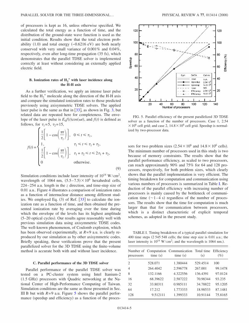
Parallel performance of the parallel TDSE solver wastested on a PC-cluster system using Intel Itanium-2�1.5 GHz� processors with Quadric networking at the Na-tional Center of High-Performance Computing of Taiwan.Simulation conditions are the same as those presented in Sec.III B but with R=9 a.u. Figure 5 shows the parallel perfor-mance �speedup and efficiency� as a function of the proces-

sors for two problem sizes �2.54�106 and 14.8�106 cells�.The minimum number of processors used in this study is twobecause of memory constraints. The results show that theparallel performance efficiency, as scaled to two processors,can reach approximately 90% and 75% for 64 and 128 pro-cessors, respectively, for both problem sizes, which clearlyshows that the parallel implementation is very efficient. Thetiming breakdown for computation and communication usingvarious numbers of processors is summarized in Table I. Re-duction of the parallel efficiency with increasing number ofprocessors is mainly caused by the bottleneck of communi-cation time ��1–4 s� regardless of the number of proces-sors. The results show that the time for computation is muchlarger than that for communication between processors,which is a distinct characteristic of explicit temporalschemes, as adopted in the present study.

FIG. 5. Parallel efficiency of the present parallelized 3D TDSEsolver as a function of the number of processors. Case 1, 2.54�106 cell grid; and case 2, 14.8�106 cell grid. Speedup is normal-ized by two-processor data.

TABLE I. Timing breakdown of a typical parallel simulation for400 time steps �2 545 548 cells; the time step size is 0.01 a.u.; thelaser intensity is 1014 W /cm2; and the wavelength is 1064 nm.�.

Number ofprocessors

Computationtime �s�

Communicationtime �s�

Total time�s�

Efficiency�%�

2 528.071 1.380444 529.4514 100

4 264.4042 2.596778 267.001 99.1478

8 132.1166 4.322556 136.4391 97.0124

16 68.39622 2.587222 70.98344 93.235

32 33.80311 0.985111 34.78822 95.1205

64 17.212 1.773333 18.98533 87.1481

128 9.512111 1.399333 10.91144 75.8165

PARALLEL SOLVER FOR THE THREE-DIMENSIONAL… PHYSICAL REVIEW A 77, 013414 �2008�

013414-5

IV. APPLICATIONS

To demonstrate the capacity of the proposed parallel 3DTDSE solver to successfully simulate a truly 3D laser-molecule interaction, a number of simulations were con-ducted. They include �1� weaker laser incidence with �=0°and 90° at R=9 a.u., where only snapshots of electron prob-ability are shown for comparison; �2� stronger laser inci-dence having different wavelengths and envelope shapeswith �=0° –90° at R=2 a.u., where the spectra of harmonicgenerations are demonstrated for comparison. In the former,the internuclear distance is intentionally chosen close towhere the ionization rate is largest, as shown in Fig. 4, whichmakes the comparison of the electron probability distributionbetween �=0° and 90° more distinct.

A. Instantaneous electron probability distribution

Important simulation conditions for a laser incident at �=0° and 90°, include a laser intensity of 1014 W /cm2, wave-length of 1064 nm, and R=9 a.u. as summarized in Table IIalong with other simulation conditions. The computationaldomain consists of �7�106 hexahedral cells, which are inturn divided into five regions with different sizes of cells. Alldomain boundaries were set with absorbing boundary condi-tions, as in the previous section. A time step of 0.01 a.u. wasused, and �105 time steps were simulated, which required12.5 h of simulation time using 32 processors on a PC clus-ter similar to that described in Sec. III C.

Figures 6 and 7 show a series of snapshots of the electronprobability distribution for �=0° and 90°, respectively, withinternuclear distance of 9 a.u.. Figure 6 shows that, when thelaser field is parallel to the molecular axis ��=0° �, initiallythe electron is driven to oscillate almost in phase with thelaser field and mostly in the z direction, as shown in Figs.6�c� and 6�d�, and is eventually ionized with high probabilityfrom the nucleus in the z direction. For example, near the endof the laser pulse �t=24.57 optical cycles�, as shown in Fig.6�f�, the electron probability near the nuclei is much smallerthan that initially �t=0�, and the total electron probability isgreatly reduced to 0.245, when ionization occurs. Similarly,Fig. 7 shows that when the laser field is perpendicular to themolecular axis ��=90° �, initially the electron is driven tooscillate almost in phase with the laser field in the y direc-tion, as shown in Figs. 7�c� and 7�d�, and is eventually ion-

ized with very low probability in the y direction �Figs. 7�a�and 7�f� are almost indistinguishable�. For example, near theend of the laser pulse �t=24.57 optical cycles�, as shown inFig. 7�f�, the total electron probability is still as high as0.858. By comparing the above two cases, we can concludethat it is much easier to ionize the H2

+ molecule if the laserfield is aligned with the molecular axis than if the laser fieldis incident in other directions. This is understandable fromthe viewpoint of classical physics, since the Coulomb forceacting on the electron due to the two nuclei is lower whenthe laser is parallel than when it is perpendicular to the mo-lecular axis, if the electron is at the same distance from themolecular center.

B. Spectra of harmonic generations

Figure 8 shows the harmonic spectra of electron probabil-ity as a function of harmonic order �up to 50� at variousangles of laser incidence with respect to the molecular axis.Note the harmonic spectrum S��� Ae���2, where Ae��� isdefined as in Eq. �3� in �10�. Important simulation conditionsinclude laser intensity of 5�1014 W /cm2, wavelength of800 nm, R=2 a.u., and various angles of incidence of �=0° –90°, as in �10�, and are summarized in Table III alongwith other simulation conditions. The laser pulse is the sameas employed in Ref. �10�, in which there are ten pulse cycleswith a sinusoidal-like envelope.. Results show that the spec-tral intensity at some specific harmonic order generally de-creases with increasing angle of laser incidence with respectto the molecular axis. In addition, the intensity decreaseswith increasing harmonic order for a fixed angle of inci-dence. Importantly, distinct peaks appear at the third, fifth,seventh, and ninth harmonic orders for angles of incidencegenerally showing a similar trend to those predicted by Ka-mta and Bandrauk �10�. However, the spectral peaks becomesmeared out at �=90° because of the much smaller ioniza-tion rate at this angle.

V. CONCLUSIONS

In the present study, a parallel solver for theCartesian-grid-based 3D TDSE with multiple nuclei and asingle active electron using the finite-volume method wasdeveloped. The validity of the parallel solver was tested by

TABLE II. Simulation conditions for weaker laser incidence onto a H2+ molecule at �=0° and 90°.

Case 1 Case 2

Angle of incidence �deg� 0 90

Laser intensity �1014 W /cm2� 1 1

Wavelength �nm� 1064 1064

Cell number 7 366 758 7 366 758

Simulation domain size �a.u.� X� 96, Y � 96, Z� 112 X� 96, Y � 96, Z� 112Time-step size �a.u.� 0.01 0.01

Internuclear distance �a.u.� 9 9

Pulse cycles 25 �88.589 fs� 25 �88.589 fs�

LEE et al. PHYSICAL REVIEW A 77, 013414 �2008�

013414-6

simulating the temporal conservation of electron probabilityand total energy of a H2

+ molecule without laser incidence,and the ionization rates of a H2

+ molecule under incidence ofa laser pulse along the H-H axis. In each case, the parallelsolver produced accurate results comparable to either ana-

lytical data or other simulation works using axisymmetriccodes in the literature. Finally, the parallel solver was appliedto simulate the response of a H2

+ molecule under laser pulseincidence at various laser field and angles of incidence to theH-H axis, which is impossible without a 3D TDSE solver.

(a) (d)

(b)

(c)

(e)

(f)

FIG. 6. �Color online� Typical snapshots of the electron probability distribution over the axisymmetric plane for a normally incidentsubfemtosecond linearly polarized laser pulse interacting with a H2

+ molecule �R=9� �power intensity is 1014 W /cm2; wavelength is1064 nm; pulse duration is 25 cycles; and angle of incidence is 0°�.

PARALLEL SOLVER FOR THE THREE-DIMENSIONAL… PHYSICAL REVIEW A 77, 013414 �2008�

013414-7

The results are generally in good agreement with previouspublished data, wherever they are available. Several studiesregarding laser-molecular interactions applying this parallelTDSE solver, which are more focused on the underlyingphysics, are currently in progress and will be presented else-

where in the near future. In addition, we aim to further de-velop the parallel 3D TDSE solver without the assumption offrozen motion of the nucleus; which allows movement of thenuclei and study of the dynamic processes during themolecule-laser interaction in a feasible way.

(a)

(b)

(c)

(d)

(e)

(f)

FIG. 7. �Color online� Typical snapshots of the electron probability distribution over the axisymmetric plane for a normally incidentsubfemtosecond linearly polarized laser pulse interacting with a H2

+ molecule �R=9� �power intensity is 1014 W /cm2; wavelength is1064 nm; pulse duration is 25 cycles; and angle of incidence is 90°�.

LEE et al. PHYSICAL REVIEW A 77, 013414 �2008�

013414-8

ACKNOWLEDGMENTS

This work was partially financially supported by the Na-tional Science Council of Taiwan through Grant No. NSC-

95-2221-E009-018. The parallel computing facility providedby the National Center for High-Performance Computing ofTaiwan is also highly appreciated.

FIG. 8. Harmonic spectra of H2+ for different orientation angles �=0–90°. Laser intensity is 5�1014 W /cm2 and wavelength is 800 nm.

Internuclear distance is 2.0 a.u.

TABLE III. Simulation conditions for stronger laser incidence onto a H2+ molecule at different angles of incidence ��=0°, 30°, 60°, and

90°�.

Case A Case B Case C Case D

Oriental angle �deg� 0 30 60 90

Laser intensity �1014 W /cm2� 5 5 5 5

Wavelength �nm� 800 800 800 800

Cell number 13 461 224 13 461 224 13 461 224 13 461 224

Simulation domain size �a.u.� X� 112Y � 112Z� 128

X� 112Y � 112Z� 128

X� 112Y � 112Z� 128

X� 112Y � 112Z� 128

Time-step size �a.u.� 0.01 0.01 0.01 0.01

Internuclear distance �a.u.� 2 2 2 2.

Pulse cycles 10 �26.6 fs� 10 �26.6 fs� 10 �26.6 fs� 10 �26.6 fs�

PARALLEL SOLVER FOR THE THREE-DIMENSIONAL… PHYSICAL REVIEW A 77, 013414 �2008�

013414-9

�1� J. H. Posthumus, Rep. Prog. Phys. 67, 623 �2004�.�2� D. Pavičic, A. Kiess, T. W. Hänsch, and H. Figger, Phys. Rev.

Lett. 94, 163002 �2005�.�3� D. Dundas, Phys. Rev. A 65, 023408 �2002�.�4� L. Y. Peng, D. Dundas, J. F. McCann, K. T. Taylor, and I. D.

Williams, J. Phys. B 36, L295 �2003�.�5� M. Vafaee and H. Sabzyan, J. Phys. B 37, 4143 �2004�.�6� M. Spanner, O. Smirnova, P. B. Corkum, and M. Y. Ivanov, J.

Phys. B 37, L243 �2004�.�7� M. V. Ivanov and R. Schinke, Phys. Rev. B 69, 165308 �2004�.�8� X. Chu and Shih-I Chu, Phys. Rev. A 63, 013414 �2000�.�9� B. Pons, Phys. Rev. A 67, 040702�R� �2003�.

�10� G. Lagmago Kamta and A. D. Bandrauk, Phys. Rev. A 70,011404�R� �2004�.

�11� G. L. Kamta and A. D. Bandrauk, Phys. Rev. A 71, 053407�2005�.

�12� G. L. Kamta and A. D. Bandrauk, Phys. Rev. Lett. 94, 203003�2005�.

�13� G. Lagmago Kamta and A. D. Bandrauk, Phys. Rev. A 74,033415 �2006�.

�14� G. Lagmago Kamta and A. D. Bandrauk, Phys. Rev. A 75,041401�R� �2007�.

�15� D. A. Telnov and Shih-I Chu, Phys. Rev. A 71, 013408 �2005�.�16� J. P. Hansen, T. Sorevik, and L. B. Madsen, Phys. Rev. A 68,

031401�R� �2003�.�17� M. Førre, S. Selstø, J. P. Hansen, and L. B. Madsen, Phys. Rev.

Lett. 95, 043601 �2005�.�18� S. Selstø, M. Førre, J. P. Hansen, and L. B. Madsen, Phys. Rev.

Lett. 95, 093002 �2005�.

�19� S. Selstø, J. F. McCann, M. Førre, J. P. Hansen, and L. B.Madsen, Phys. Rev. A 73, 033407 �2006�.

�20� T. K. Kjeldsen, L. B. Madsen, and J. P. Hansen, Phys. Rev. A74, 035402 �2006�.

�21� Barry I. Schneider and L. A. Collins, J. Non-Cryst. Solids 351,1551 �2005�.

�22� S. X. Hu and L. A. Collins, Phys. Rev. Lett. 94, 073004�2005�.

�23� S. X. Hu and L. A. Collins, Phys. Rev. A 73, 023405 �2006�.�24� S. X. Hu and L. A. Collins, J. Phys. B 73, L185 �2006�.�25� B. I. Schneider, L. A. Collins, and S. X. Hu, Phys. Rev. E 73,

036708 �2006�.�26� H. Yu and A. D. Bandrauk, J. Chem. Phys. 102, 1257 �1995�.�27� H. K. Versteeg and W. Malasekera, An Introduction to Com-

putational Fluid Dynamics: The Finite Volume Method�Addison-Wesley/Longman, Harlow, U.K., 1995�.

�28� P. B. Visscher, Comput. Phys. 5, 596 �1991�.�29� Y. M. Lee, T. F. Jiang, and J. S. Wu, in Proceedings of the

Fourth International Conference on Quantum Engineering Sci-ence, Tainan, Taiwan, 2006.

�30� J. G. L. Booten, H. A. van der Vorst, P. M. Meijer, and H. J. J.te Riele, CWI Report No. NM-R9414, 1994 �unpublished�.

�31� Daniel Dundas, J. F. McCann, Jonathan S. Parker, and K. T.Taylor, J. Phys. B 33, 3261 �2000�.

�32� George Karypis and Vipin Kumar, SIAM J. Sci. Comput.�USA� 20, 359 �1999�.

�33� Mohsen Vafaee, Hassan Sabzyan, Zahra Vafaee, and Ali Ka-tanforoush, Phys. Rev. A 74, 043416 �2006�.

LEE et al. PHYSICAL REVIEW A 77, 013414 �2008�

013414-10