Embed Size (px)
Citation preview
Parallel Sorting on the HeterogeneousAMD Fusion Accelerated Processing Unit
by
Michael Christopher Delorme
A thesis submitted in conformity with the requirementsfor the degree of Master of Applied Science
Graduate Department of Electrical and Computer EngineeringUniversity of Toronto
Copyright c© 2013 by Michael Christopher Delorme
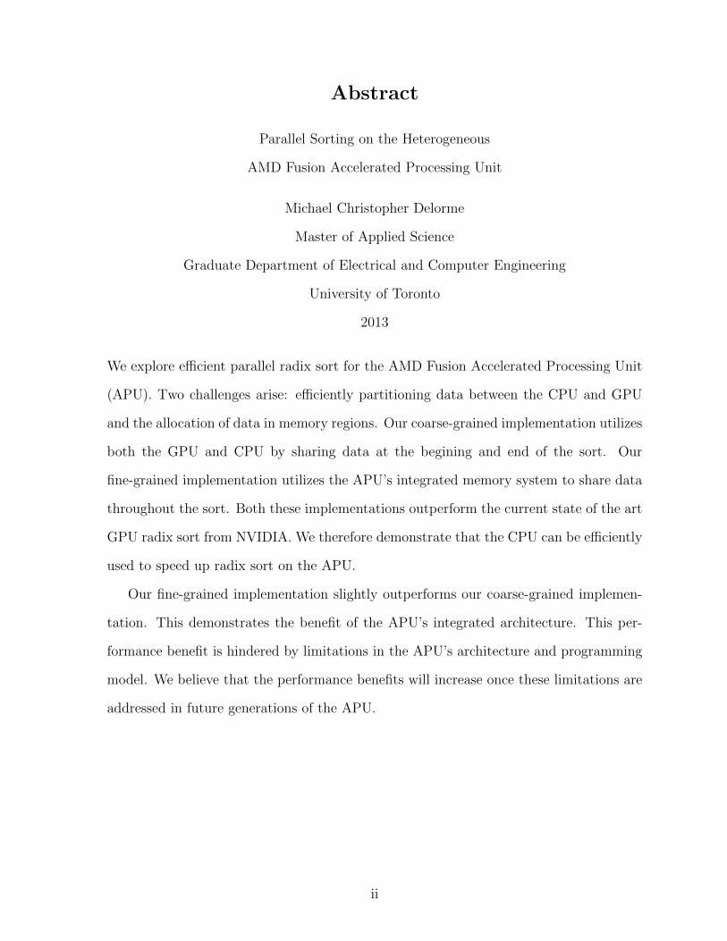
Abstract
Parallel Sorting on the Heterogeneous
AMD Fusion Accelerated Processing Unit
Michael Christopher Delorme
Master of Applied Science
Graduate Department of Electrical and Computer Engineering
University of Toronto
2013
We explore efficient parallel radix sort for the AMD Fusion Accelerated Processing Unit
(APU). Two challenges arise: efficiently partitioning data between the CPU and GPU
and the allocation of data in memory regions. Our coarse-grained implementation utilizes
both the GPU and CPU by sharing data at the begining and end of the sort. Our
fine-grained implementation utilizes the APU’s integrated memory system to share data
throughout the sort. Both these implementations outperform the current state of the art
GPU radix sort from NVIDIA. We therefore demonstrate that the CPU can be efficiently
used to speed up radix sort on the APU.
Our fine-grained implementation slightly outperforms our coarse-grained implemen-
tation. This demonstrates the benefit of the APU’s integrated architecture. This per-
formance benefit is hindered by limitations in the APU’s architecture and programming
model. We believe that the performance benefits will increase once these limitations are
addressed in future generations of the APU.
ii
Dedication
This thesis is lovingly dedicated to my dear mother, Daniela Belluz-Delorme.
Thank you for twenty wonderful years of love, care, and encouragement.
Gone now but never forgotten, I will miss you always.
iii

Acknowledgements
First and foremost, I would like to thank my thesis supervisor, Professor Tarek S. Ab-
delrahman. He has provided a level of patience, encouragement, and insight that has
has been invaluable to my academic development. His feedback and expertise have have
helped guide me through my research.
I have taken several courses during graduate school that have provided me with
the necessary background to undertake this research. I would therefore like to thank
professors Andreas Moshovos, Gregory Steffan, and Natalie Enright Jerger. Additional
thanks go to professors Andreas Moshovos, Gregory Steffan, and Konstantinos Plataniotis
for acting as members of my M.A.Sc. committee.
I would like to extend my gratitude to fellow graduate student David Han. In addition
to providing me with a great deal of feedback on my work, he has also given me a great
deal of support and perspective when research was looking bleak.
I owe my parents and grandparents a debt of gratitude that I am certain I will never
be able to repay. Special thanks go to my caring father Michael J. Delorme and my loving
partner Karley Hatherell. I would not have been able to complete this work without their
unfailing love and support.
iv

Contents
1 Introduction 1
1.1 Thesis Overview . . . . . . . . . . . . . . . . . . . . . . . . . . . . . . . . 2
1.2 Thesis Contributions . . . . . . . . . . . . . . . . . . . . . . . . . . . . . 3
1.3 Thesis Organization . . . . . . . . . . . . . . . . . . . . . . . . . . . . . . 4
2 The AMD Fusion Accelerated Processing Unit 5
2.1 Hardware Overview . . . . . . . . . . . . . . . . . . . . . . . . . . . . . . 5
2.1.1 CPU Hardware . . . . . . . . . . . . . . . . . . . . . . . . . . . . 6
2.1.2 GPU Hardware . . . . . . . . . . . . . . . . . . . . . . . . . . . . 8
2.2 Memory Access and Allocation . . . . . . . . . . . . . . . . . . . . . . . 8
2.2.1 CPU Accesses to Cached Host Memory . . . . . . . . . . . . . . . 9
2.2.2 CPU Accesses to Uncached Host Memory . . . . . . . . . . . . . 9
2.2.3 CPU Accesses to Device-Visible Host Memory . . . . . . . . . . . 9
2.2.4 GPU Accesses to Cached Host Memory . . . . . . . . . . . . . . . 10
2.2.5 GPU Accesses to Uncached Host Memory . . . . . . . . . . . . . 10
2.2.6 GPU Accesses to Device-Visible Host Memory . . . . . . . . . . . 10
3 Programming the Fusion Accelerated Processing Unit 11
3.1 OpenCL . . . . . . . . . . . . . . . . . . . . . . . . . . . . . . . . . . . . 11
3.1.1 Platform Model . . . . . . . . . . . . . . . . . . . . . . . . . . . . 11
3.1.2 Execution Model . . . . . . . . . . . . . . . . . . . . . . . . . . . 13
v
3.1.3 Memory Model . . . . . . . . . . . . . . . . . . . . . . . . . . . . 18
3.1.4 Programming Model . . . . . . . . . . . . . . . . . . . . . . . . . 21
3.2 OpenCL on the AMD Fusion APU . . . . . . . . . . . . . . . . . . . . . 22
3.2.1 Programming the GPU in OpenCL . . . . . . . . . . . . . . . . . 23
3.2.2 Programming the CPU in OpenCL . . . . . . . . . . . . . . . . . 23
3.2.3 Buffer Mapping on the AMD Fusion Platform . . . . . . . . . . . 24
4 Radix Sort 26
4.1 Sequential Algorithm Overview . . . . . . . . . . . . . . . . . . . . . . . 26
4.2 Parallel Radix Sort Algorithm . . . . . . . . . . . . . . . . . . . . . . . . 31
5 Fusion Sort 41
5.1 Motivation . . . . . . . . . . . . . . . . . . . . . . . . . . . . . . . . . . . 41
5.2 Coarse-Grained Algorithm . . . . . . . . . . . . . . . . . . . . . . . . . . 43
5.3 Fine-Grained Static Algorithm . . . . . . . . . . . . . . . . . . . . . . . . 45
5.4 Fine-Grained Dynamic Algorithm . . . . . . . . . . . . . . . . . . . . . . 48
5.5 Summary . . . . . . . . . . . . . . . . . . . . . . . . . . . . . . . . . . . 49
6 Implementation 51
6.1 GPU-Only Implementation . . . . . . . . . . . . . . . . . . . . . . . . . . 51
6.2 CPU-Only Implementation . . . . . . . . . . . . . . . . . . . . . . . . . . 52
6.3 Coarse-Grained Implementation . . . . . . . . . . . . . . . . . . . . . . . 57
6.4 Fine-Grained Static Implementation . . . . . . . . . . . . . . . . . . . . . 59
6.5 Fine-Grained Static Split Scatter Implementation . . . . . . . . . . . . . 61
6.6 Fine-Grained Dynamic Implementation . . . . . . . . . . . . . . . . . . . 62
6.7 Theoretical Optimum Model . . . . . . . . . . . . . . . . . . . . . . . . . 64
7 Evaluation 66
7.1 Hardware Platforms . . . . . . . . . . . . . . . . . . . . . . . . . . . . . 66
vi
7.2 Software Platform . . . . . . . . . . . . . . . . . . . . . . . . . . . . . . . 67
7.3 Performance Metrics . . . . . . . . . . . . . . . . . . . . . . . . . . . . . 68
7.4 Evaluated Implementations . . . . . . . . . . . . . . . . . . . . . . . . . 69
7.5 GPU-Only Results . . . . . . . . . . . . . . . . . . . . . . . . . . . . . . 70
7.6 CPU-Only Results . . . . . . . . . . . . . . . . . . . . . . . . . . . . . . 72
7.7 Coarse-Grained Results . . . . . . . . . . . . . . . . . . . . . . . . . . . . 76
7.8 Fine-Grained Static Results . . . . . . . . . . . . . . . . . . . . . . . . . 81
7.9 Fine-Grained Static Split Scatter Results . . . . . . . . . . . . . . . . . . 86
7.10 Fine-Grained Dynamic Results . . . . . . . . . . . . . . . . . . . . . . . . 91
7.11 Impact of Memory Allocation . . . . . . . . . . . . . . . . . . . . . . . . 94
7.12 Comparative Performance . . . . . . . . . . . . . . . . . . . . . . . . . . 98
8 Related Work 102
9 Conclusions and Future Work 105
9.1 Future Work . . . . . . . . . . . . . . . . . . . . . . . . . . . . . . . . . . 106
Bibliography 109
vii

List of Tables
3.1 OpenCL memory allocation and access capabilities by region. . . . . . . . 18
6.1 Table of GPU-Only kernel launch parameters. . . . . . . . . . . . . . . . 52
6.2 Table of CPU-Only kernel input tile sizes. . . . . . . . . . . . . . . . . . 53
6.3 Memory buffer allocation details for the Fine-Grained Static implementation. 60
6.4 Memory buffer allocation details for the Fine-Grained Dynamic implemen-
tation. . . . . . . . . . . . . . . . . . . . . . . . . . . . . . . . . . . . . . 63
7.1 Summary of evaluation platforms. . . . . . . . . . . . . . . . . . . . . . . 67
7.2 Optimal per-kernel partition points for the Fine-Grained Dynamic imple-
mentation. . . . . . . . . . . . . . . . . . . . . . . . . . . . . . . . . . . . 92
viii
List of Figures
2.1 An overview of the Llano APU hardware. . . . . . . . . . . . . . . . . . . 6
3.1 The OpenCL Platform Model. . . . . . . . . . . . . . . . . . . . . . . . . 12
3.2 An example of an NDRange index space. . . . . . . . . . . . . . . . . . . 15
3.3 The OpenCL Memory Model. . . . . . . . . . . . . . . . . . . . . . . . . 19
3.4 Zero copy buffer mapping on the AMD Llano architecture. . . . . . . . . 24
4.1 An example of a set of values being sorted from least to most significant
digit. . . . . . . . . . . . . . . . . . . . . . . . . . . . . . . . . . . . . . . 27
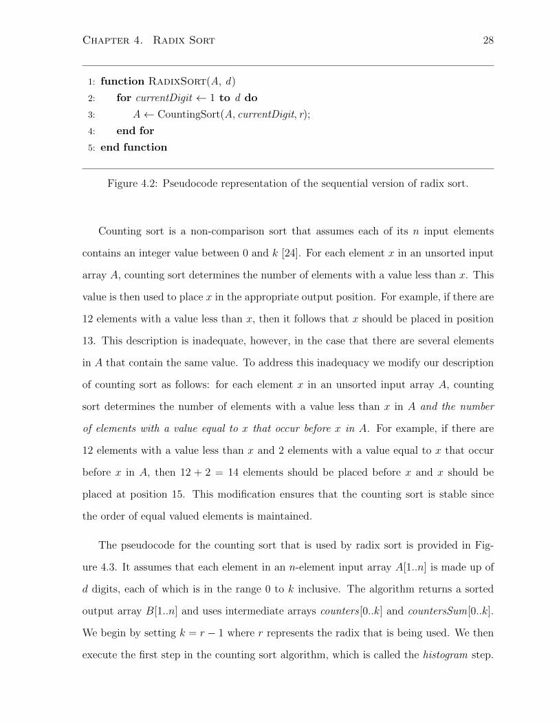
4.2 Pseudocode representation of the sequential version of radix sort. . . . . 28
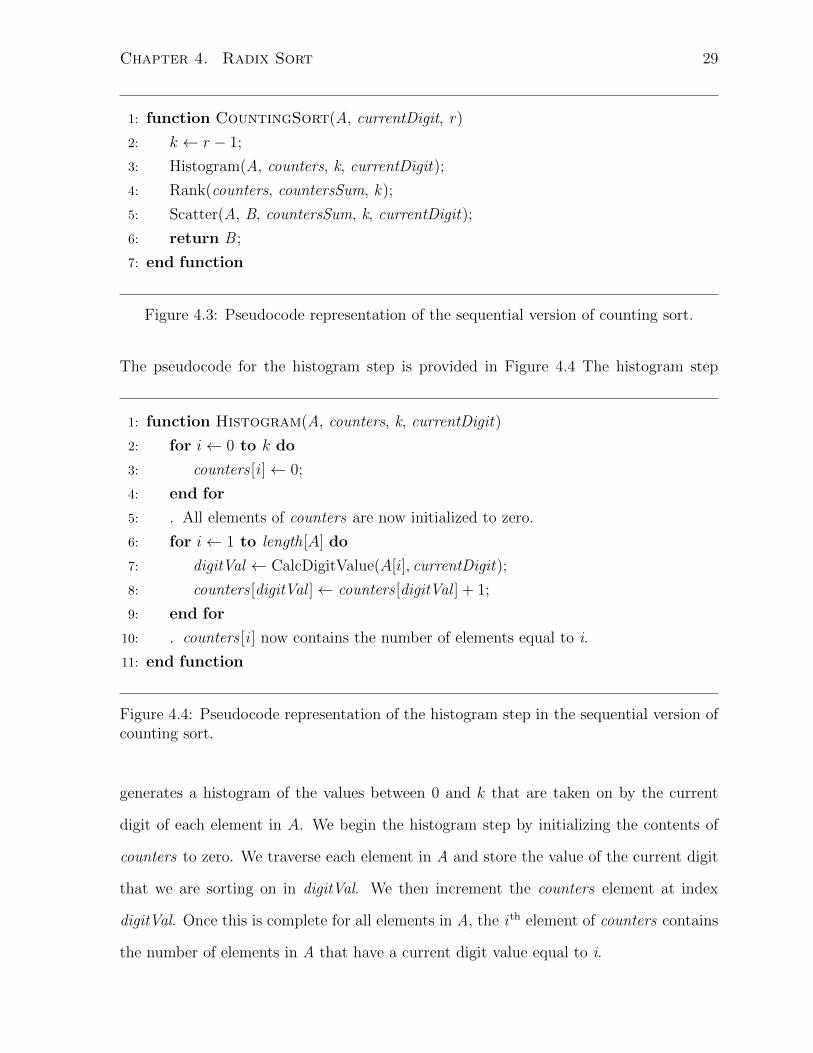
4.3 Pseudocode representation of the sequential version of counting sort. . . . 29
4.4 Pseudocode representation of the histogram step in the sequential version
of counting sort. . . . . . . . . . . . . . . . . . . . . . . . . . . . . . . . . 29
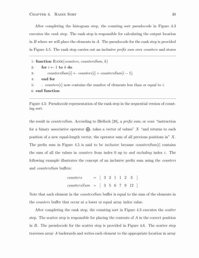
4.5 Pseudocode representation of the rank step in the sequential version of
counting sort. . . . . . . . . . . . . . . . . . . . . . . . . . . . . . . . . . 30
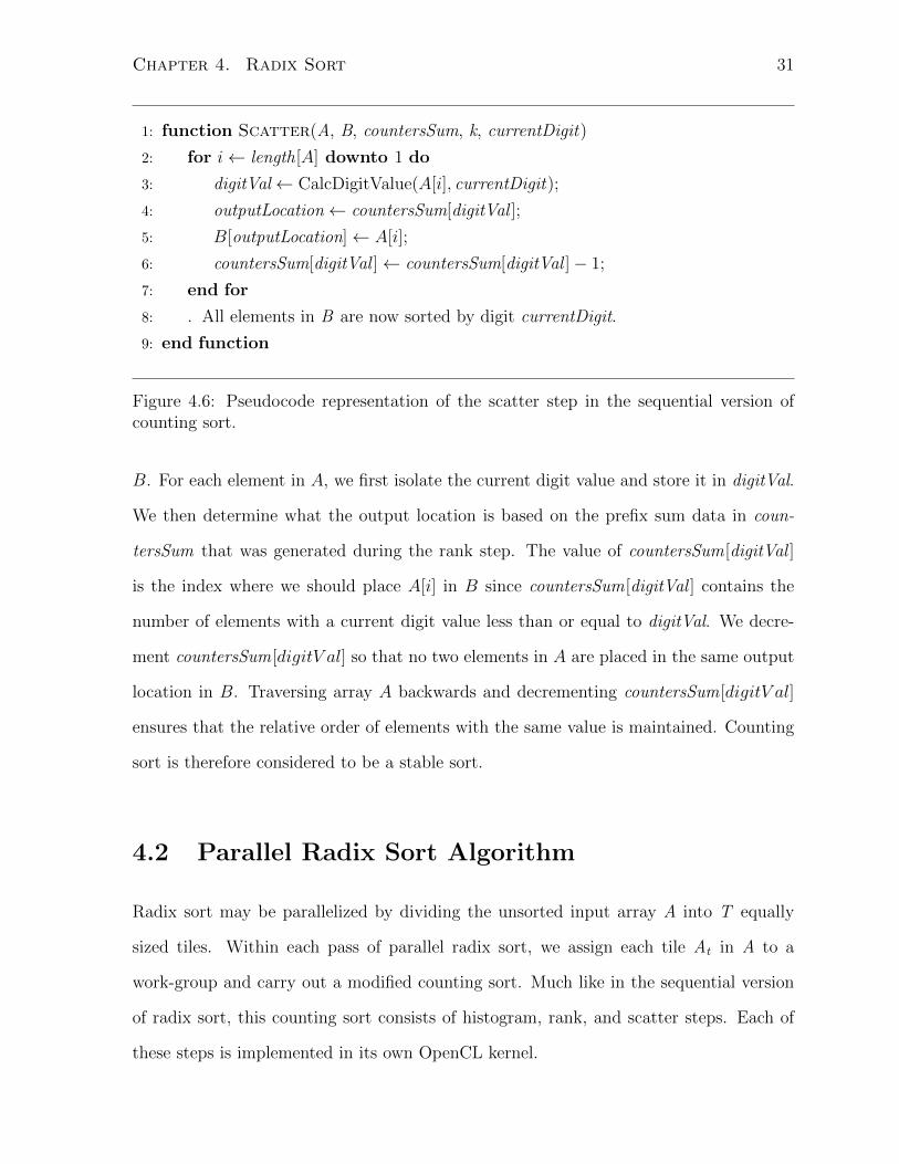
4.6 Pseudocode representation of the scatter step in the sequential version of
counting sort. . . . . . . . . . . . . . . . . . . . . . . . . . . . . . . . . . 31
4.7 The counters buffer is stored in column-major order for the prefix sum
operation. . . . . . . . . . . . . . . . . . . . . . . . . . . . . . . . . . . . 33
4.8 Pseudocode representation of the parallel version of radix sort. . . . . . . 34
4.9 Pseudocode representation of the parallel local sort kernel. . . . . . . . . 35
ix
4.10 An example of a 1-bit split operation being carried on an array of values
using each element’s least significant bit. . . . . . . . . . . . . . . . . . . 35
4.11 An illustration of the contiguous regions of equally-valued elements that
are generated in the local sort step. . . . . . . . . . . . . . . . . . . . . . 36
4.12 Pseudocode representation of the parallel histogram kernel. . . . . . . . . 37
4.13 Pseudocode representation of the parallel scatter kernel. . . . . . . . . . 39
5.1 Pseudocode representation of the Coarse-Grained algorithm. . . . . . . . 44
5.2 Pseudocode representation of the Fine-Grained Static algorithm. . . . . . 46
5.3 Pseudocode representation of the Fine-Grained Dynamic algorithm. . . . 48
5.4 A taxonomy of each algorithm with respect to the partitioning method,
data sharing granularity and memory allocation method. . . . . . . . . . 50
6.1 Pseudocode of the local sort kernel in the CPU-Only implementation. . . 54
6.2 Pseudocode of the histogram kernel in the CPU-Only implementation. . . 55
6.3 Pseudocode of the rank kernel in the CPU-Only implementation. . . . . . 56
6.4 Pseudocode of the scatter kernel in the CPU-Only implementation. . . . 56
6.5 Pseudocode of the merge kernel in the Coarse-Grained implementation. . 58
6.6 An example illustrating how the theoretical optimum execution time and
partition point are determined. . . . . . . . . . . . . . . . . . . . . . . . 65
7.1 Sort time of the GPU-Only implementation on the A6-3650 and A8-3850. 70
7.2 The GPU-Only per-kernel execution time as a percent of all kernel execu-
tion time. . . . . . . . . . . . . . . . . . . . . . . . . . . . . . . . . . . . 71
7.3 Throughput of the GPU-Only and NVIDIA reference implementation on
the A6-3650 and A8-3850. . . . . . . . . . . . . . . . . . . . . . . . . . . 72
7.4 Sort time of the CPU-Only implementation on the A6-3650 as a function
of input dataset size. . . . . . . . . . . . . . . . . . . . . . . . . . . . . . 73
x
7.5 Sort time of the CPU-Only implementation on the A8-3850 as a function
of input dataset size. . . . . . . . . . . . . . . . . . . . . . . . . . . . . . 73
7.6 Throughput of the CPU-Only implementation sorting 128 Mi unsigned
integer values across a varying number of threads on the A6-3650 and the
A8-3850 platforms. . . . . . . . . . . . . . . . . . . . . . . . . . . . . . . 74
7.7 Sort time of the CPU-Only implementation on the A6-3650 and A8-3850. 75
7.8 The CPU-Only per-kernel execution time as a percent of all execution time. 75
7.9 Sort time of the Coarse-Grained implementation on the A6-3650 as a func-
tion of input dataset partitioning. . . . . . . . . . . . . . . . . . . . . . . 77
7.10 Sort time of the Coarse-Grained implementation on the A8-3850 as a func-
tion of input dataset partitioning. . . . . . . . . . . . . . . . . . . . . . . 77
7.11 Sort time of the Coarse-Grained implementation on the A6-3650 and A8-
3850. . . . . . . . . . . . . . . . . . . . . . . . . . . . . . . . . . . . . . . 79
7.12 Sort time of the Coarse-Grained implementation on the A6-3650 and A8-
3850 with and without the final merge step. . . . . . . . . . . . . . . . . 80
7.13 Merge time of the Coarse-Grained implementation on the A6-3650 and
A8-3850 as a function of the GPU partition point. . . . . . . . . . . . . . 80
7.14 Sort time of the Fine-Grained Static implementation on the A6-3650 as a
function of input dataset partitioning. . . . . . . . . . . . . . . . . . . . . 82
7.15 Sort time of the Fine-Grained Static implementation on the A8-3850 as a
function of input dataset partitioning. . . . . . . . . . . . . . . . . . . . . 82
7.16 Per-kernel idle time found in the Fine-Grained Static implementation on
the A6-3650. . . . . . . . . . . . . . . . . . . . . . . . . . . . . . . . . . . 84
7.17 Per-kernel idle time found in the Fine-Grained Static implementation on
the A8-3850. . . . . . . . . . . . . . . . . . . . . . . . . . . . . . . . . . . 84
7.18 Sort time of the Fine-Grained Static implementation on the A6-3650 and
the A8-3850 as a function of input dataset partitioning. . . . . . . . . . . 86
xi

7.19 Sort time of the Fine-Grained Split Scatter implementation as a function
of input dataset size on the A6-3650. . . . . . . . . . . . . . . . . . . . . 87
7.20 Sort time of the Fine-Grained Static Split Scatter implementation as a
function of input dataset size on the A8-3850. . . . . . . . . . . . . . . . 87
7.21 Sort time of the Fine-Grained Split Scatter implementation on the A6-3650
and A8-3850. . . . . . . . . . . . . . . . . . . . . . . . . . . . . . . . . . 88
7.22 Per-kernel idle time found in the Fine-Grained Static Split Scatter imple-
mentation on the A6-3650. . . . . . . . . . . . . . . . . . . . . . . . . . . 89
7.23 Per-kernel idle time found in the Fine-Grained Static Split Scatter imple-
mentation on the A8-3850. . . . . . . . . . . . . . . . . . . . . . . . . . . 90
7.24 The sum of the per-kernel idle times found in the Fine-Grained Static Split
Scatter implementation on the A6-3650 and A8-3850. . . . . . . . . . . . 91
7.25 The sort time of the Fine-Grained Dynamic partitioning implementation
over a varying number of threads on the A6-3650 and the A8-3850 . . . . 92
7.26 The sort time of the Fine-Grained Dynamic partitioning implementation
as the per-kernel partitioning varies on the A6-3650. . . . . . . . . . . . . 93
7.27 The sort time of the Fine-Grained Dynamic partitioning implementation
as the per-kernel partitioning varies on the A8-3850. . . . . . . . . . . . . 94
7.28 Speedup resulting from the algorithmic complexity of managing multiple
devices and buffers in the Fine-Grained Dynamic implementation. . . . . 96
7.29 Speedup resulting from alternate memory allocation strategies in the Fine-
Grained Dynamic implementation. . . . . . . . . . . . . . . . . . . . . . 97
7.30 Maximum sorting throughput of each implementation on the A6-3650 and
the A8-3850. . . . . . . . . . . . . . . . . . . . . . . . . . . . . . . . . . . 99
7.31 Speedup with respect to the NVIDIA reference implementation on the
A6-3650 and the A8-3850. . . . . . . . . . . . . . . . . . . . . . . . . . . 100
xii
Chapter 1
Introduction
Over the past decade there has been a considerable amount of interest in computer
architectures that consist of many processing cores [30]. Examples of such architectures
include graphics processing units (GPUs), the Intel Single-Chip Cloud Computer [17],
and the Intel Many Integrated Core Architecture [13]. These many-core platforms have
the potential to offer more processing capability while using less power than traditional
processors [30].
GPU devices are commonly in the form of discrete graphics cards that are attached
to the computing system via a Peripheral Component Interconnect Express (PCI-E) bus.
These discrete cards contain some form of dedicated dynamic random access memory
(DRAM) that acts as the GPU’s primary memory region. This is a separate memory from
the main system DRAM that is used by the central processing unit (CPU). This makes
it necessary to first allocate a region of memory in the GPU’s DRAM and copy pertinent
data from the CPU’s memory to the GPU’s memory [30]. Once this is complete, the GPU
executes a program or kernel, that operates upon this data. Once the kernel execution
has completed, any data generated by the GPU is then copied back from the GPU’s
memory to the CPU’s memory. Since the GPU and CPU have separate physical DRAMs
and copying data across the PCI-E bus can typically take a considerable amount of time,
1
Chapter 1. Introduction 2
the CPU often remains idle and therefore underutilized during GPU kernel execution.
A new computing architecture was recently released by Advanced Micro Devices
(AMD) called the AMD Fusion Accelerated Processing Unit (APU). This architecture
integrates a CPU and GPU onto a single silicon die and allows both devices to share
the same physical DRAM. This architecture appears promising since it has the potential
to reduce data transfer time between the CPU and GPU. It is, however, unclear just
how beneficial this architecture is to the area of general-purpose computing. It is also
unclear how suitable the existing OpenCL programming model, which is commonly used
to program GPU devices, is to these new APU platforms. In this thesis we answer these
questions in the context of parallel sorting. We are motivated to consider sorting because
it is a well known problem that is important in the area of computer science. Radix sort
has already been efficiently implemented on GPU devices by Satish et al. [36], however
there does not exist an implementation that efficiently utilizes both the CPU and GPU
simultaneously.
1.1 Thesis Overview
We have studied the radix sort algorithm described by Satish et al. [36] and have adapted
it for execution on both the CPU and GPU components of the AMD Fusion APU. Two
challenges arise in doing so: (i) efficiently partitioning and sharing data between the CPU
and GPU and (ii) determining the optimal memory region in which to store data. We
have developed a version of radix sort in which very little data sharing takes place between
the on-chip CPU and GPU. This version is called the Coarse-Grained algorithm. We have
also developed several versions of radix sort in which there is a relatively large amount of
data sharing between the CPU and GPU devices. These versions make use of the APU’s
integrated architecture to provide fast data sharing between the GPU and CPU. We call
these versions our Fine-Grained algorithms. We have implemented and benchmarked

Chapter 1. Introduction 3
these algorithms on two AMD Fusion APU models. Both of these algorithms execute
faster than the original algorithm presented by Satish et al. [36], thereby demonstrating
that it is possible to use the CPU to efficiently speed up radix sort on the APU.
The results indicate that the Fine-Grained algorithm executes slightly faster than the
Coarse-Grained algorithm, thereby demonstrating the benefit of the APU’s integrated
architecture. These benefits are, however, limited by the Fusion APU’s architecture and
programming model. We quantify the degree to which these limitations impact the per-
formance of the Fine-Grained algorithm through a series of experiments. We determine
that these limitations impose a significant performance penalty on the algorithm and
make recommendations for future generations of the APU hardware and software.
1.2 Thesis Contributions
In this thesis we make the following contributions:
1. We have provided the first sorting algorithms to efficiently make use of both the
GPU and CPU simultaneously.
2. We have implemented and evaluated these algorithms on multiple APU models in
order to better characterize their performance capabilities. Our work shows that
workload partitioning is a suitable method of parallelizing radix sort on the AMD
Fusion APU. We have also demonstrated that repartitioning this workload at each
step of the sorting algorithm is beneficial to performance.
3. We demonstrate that the a fine-grained data sharing approach is beneficial to the
performance of radix sort on the Fusion APU. In doing so, we expose the limitations
of the APU’s architecture and programming model that hinder performance under
fine-grained data sharing scenarios.
Chapter 1. Introduction 4
1.3 Thesis Organization
The remainder of the thesis is organized as follows. Chapter 2 details the hardware ar-
chitecture of the AMD Fusion APU. This is followed by a description of the OpenCL
programming model that is used to program the APU in Chapter 3. Chapter 4 describes
both the sequential version of radix sort as well as the parallel version of radix sort that
is presented by Satish et al. [36]. In Chapter 5 we describe the algorithmic overview of
our Coarse-Grained and Fine-Grained variants of radix sort. We provide the implemen-
tation details for these radix sort variants in Chapter 6. Each of the implementations is
evaluated in Chapter 7. A survey of related work is provided in Chapter 8. Finally, in
Chapter 9 we present concluding remarks and recommendations for future work.

Chapter 2
The AMD Fusion Accelerated
Processing Unit
We begin this chapter by describing the hardware characteristics of the AMD Fusion
accelerated processing unit. Both the on-chip GPU and CPU devices are detailed. We
then present the various memory regions that are available and describe how the CPU
and GPU access them.
2.1 Hardware Overview
The Advanced Micro Devices (AMD) Fusion accelerated processing unit (APU) is a het-
erogeneous computing environment that integrates scalar and vector compute engines
onto a single silicon die [4, 23]. The scalar compute engine is comprised of a multi-core
central processing unit (CPU) while a graphics processing unit (GPU) acts as the corre-
sponding vector compute engine. The current generation of Fusion APU is codenamed
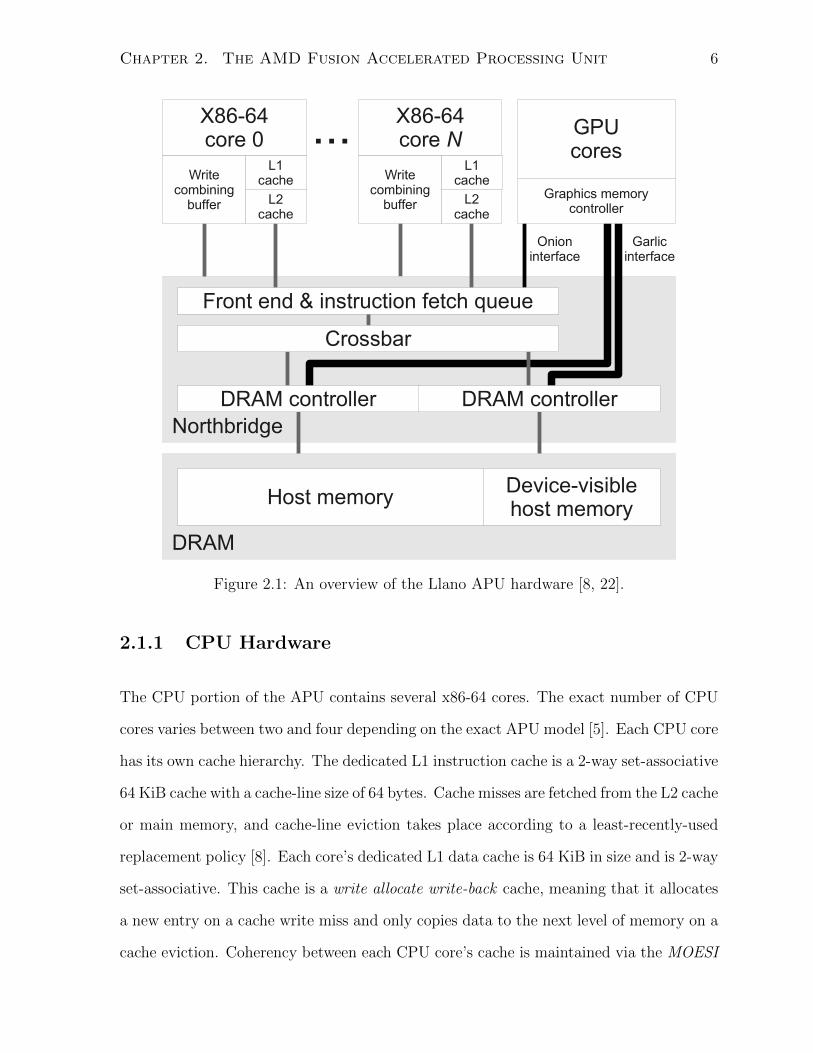
Llano [22] and its high-level organization is depicted in Figure 2.1. The CPU and GPU
components both utilize the same main system memory (DRAM) pool to provide mem-
ory to each device. This differs from traditional CPU and discrete GPU combinations
where each device has its own dedicated DRAM.
5
Chapter 2. The AMD Fusion Accelerated Processing Unit 6
Northbridge
X86-64core 0 ... X86-64
core NGPUcores
DRAM
Host memory Device-visible host memory
Onion interface
Garlic interface
Write combining
buffer L2 cache
Write combining
buffer L2 cache
Graphics memory controller
Front end & instruction fetch queue
Crossbar
DRAM controller DRAM controller
L1 cache
L1 cache
Figure 2.1: An overview of the Llano APU hardware [8, 22].
2.1.1 CPU Hardware
The CPU portion of the APU contains several x86-64 cores. The exact number of CPU
cores varies between two and four depending on the exact APU model [5]. Each CPU core
has its own cache hierarchy. The dedicated L1 instruction cache is a 2-way set-associative
64 KiB cache with a cache-line size of 64 bytes. Cache misses are fetched from the L2 cache
or main memory, and cache-line eviction takes place according to a least-recently-used
replacement policy [8]. Each core’s dedicated L1 data cache is 64 KiB in size and is 2-way
set-associative. This cache is a write allocate write-back cache, meaning that it allocates
a new entry on a cache write miss and only copies data to the next level of memory on a
cache eviction. Coherency between each CPU core’s cache is maintained via the MOESI
Chapter 2. The AMD Fusion Accelerated Processing Unit 7
(Modified, Owner, Exclusive, Shared, and Invalid) cache-coherency protocol [8].
Each CPU core has its own general-purpose L2 cache that is not shared amongst the
other cores. This cache features an exclusive cache architecture, meaning that it only
contains cache blocks that were evicted from the L1 cache. The L2 cache is 1024 KiB in
size and is 16-way set associative. No form of L3 cache is present on the chip [8].
It is important to note that throughout this document cached memory refers to a
region of memory that is accessed via the CPU’s cache hierarchy. Similarly, uncached
memory refers to a region of memory that is not accessed via the CPU’s cache hierarchy.
Each CPU core also has a write combining buffer. The buffer is used to combine
multiple memory-write operations that are performed to uncached memory. In order to
effectively utilize the write combining buffer, the memory addresses that are written to
must fall within the same 64-byte memory region that is aligned to a cache-line boundary.
Scattered writes that do not fall within the same 64-byte cache-aligned region will cause
the buffer to flush its data before it is full [8].
Each core’s cache hierarchy accesses memory via the on-die northbridge, specifically
the front end and instruction fetch queues. The front end is responsible for maintaining
coherency and consistency across memory accesses, while the instruction fetch queue is
the centralized queue that holds cacheable traffic. The front end and instruction fetch
queues communicate with the available DRAM controllers via a crossbar switch [8]. The
Llano architecture has two integrated DRAM controllers. Each controller accesses DRAM
memory via its own independent 64-bit memory channel [6]. The Llano APU supports
DDR3 memory at speeds up to 1866 MHz [5]. The write combining buffers also access
memory via the northbridge, however they do not make use of the front end coherency
logic [8].
Chapter 2. The AMD Fusion Accelerated Processing Unit 8
2.1.2 GPU Hardware
The GPU portion of the Llano APU contains several graphics cores which AMD refers
to as Radeon cores [5] or GPU cores. Much like the number of CPU cores, the number of
Radeon cores varies from 160 cores on the A4-3300 model to 400 cores on the A8-3870K
model [5].
As shown in Figure 2.1, the GPU’s graphics memory controller is able to access
memory via two different interfaces. The Garlic interface allows the graphics memory
controller to access the DRAM controllers directly. This provides the GPU access to
uncached memory. Note that the Garlic interface is replicated for each of the available
DRAM controllers. The Onion interface allows the graphics memory controller to access
memory via the same front end and instruction fetch queue that the CPU cache hierarchy
uses. This provides the GPU access to cached memory while maintaining cache coherency
with the CPU’s cache hierarchy [8].
2.2 Memory Access and Allocation
The main system memory is logically partitioned between the APU’s on-die CPU and
GPU. This is achieved by assigning each device its own virtual address space. The
CPU’s and GPU’s virtual memory regions are respectively referred to as host memory
and device-visible host memory. It is important to note that device-visible host memory
is always uncached with respect to the CPU’s cache hierarchy. In contrast, host memory
may be designated as either cached or uncached at allocation time. It is currently not
possible to change the caching designation of a host memory region once it has been
allocated [3].
Chapter 2. The AMD Fusion Accelerated Processing Unit 9
2.2.1 CPU Accesses to Cached Host Memory
The CPU accesses cached host memory via its L1 and L2 cache hierarchy [8]. This
provides the fastest read/write path between the CPU and the on-chip DRAM controllers.
As such, this memory region is referred to as the CPU’s preferred memory region. Single
threaded performance has been measured at 8 GB/s for reads and writes, while multi-
threaded performance has been measured at 13 GB/s [22].
2.2.2 CPU Accesses to Uncached Host Memory
CPU writes to uncached host memory are performed using the available write combin-
ing buffers. This provides relatively fast streaming write access to memory [3]. Multi-
threaded writes can be used to improve bandwidth using multiple CPU cores. This is
because each core has its own write combining buffer. Multi-threaded writes have been
measured at up to 13 GB/s. However, both single-threaded and multi-threaded reads
are very slow because they are uncached [22].
2.2.3 CPU Accesses to Device-Visible Host Memory
Both the CPU and the GPU are capable of accessing each other’s virtual memories.
The CPU is able to access device-visible host memory by mapping a device-visible host
memory region into the CPU’s virtual address space. Since device-visible host memory is
uncached, writes take place using the CPU’s write combining buffer. Instead of writing
directly to the DRAM controllers, the write combining buffers send the data over the
Onion interface to the GPU’s graphics memory controller. The GPU’s graphics memory
controller is then responsible for writing the data to memory over the Garlic interface.
CPU reads from device-visible host memory are accessed via the Onion interface in a
similar manner. CPU writes can peak at 8 GB/sec, while reads are very slow due to
the fact that this memory region is uncached. Note that on systems with discrete cards,
Chapter 2. The AMD Fusion Accelerated Processing Unit 10
CPU writes to GPU memory are limited to 6 GB/s by the PCIe bus [22].
2.2.4 GPU Accesses to Cached Host Memory
The GPU is able to access host memory regions by mapping a host memory region into
the GPU’s virtual address space. The GPU must maintain cache coherency with the CPU
when accessing this type of memory. As a result, GPU reads and writes take place over
the Onion interface. Accessing memory through this interface ensures that GPU reads
and writes remain cache coherent with respect to the CPU’s cache hierarchy. This cache
coherent access comes at a cost, however. GPU reads and writes are now subject to the
same cache coherency protocol as CPU reads and writes. This has potential to introduce
cache invalidations and increase on-chip network traffic. Reads have been measured at
4.5 GB/s, while writes can take place at up to 5.5 GB/s [22].
2.2.5 GPU Accesses to Uncached Host Memory
Similar to cached host memory, the GPU is able to access uncached host memory once
it has been mapped into the GPU’s virtual address space. Accesses to uncached host
memory takes place via the Garlic interface. GPU accesses to uncached host memory
operate slightly slower than accesses to device-visible host memory. Reads have been
measured at up to 12 GB/s [22].
2.2.6 GPU Accesses to Device-Visible Host Memory
The GPU accesses device-visible host memory via the Garlic interface [8] (see Figure 2.1).
This provides the fastest read/write path between the GPU and the on-chip DRAM
controllers and is referred to as the GPU’s preferred memory region. GPU access to this
memory region has been measured at 17 GB/s for reads and 13 GB/s for writes [22].
Chapter 3
Programming the Fusion
Accelerated Processing Unit
In this chapter we present the OpenCL programming model for the AMD Fusion Acceler-
ated Processing Unit. We begin by describing the various models that are provided by the
OpenCL framework. We then describe relevant details of how the OpenCL programming
model maps to the hardware of the Fusion Accelerated Processing Unit.
3.1 OpenCL
OpenCL is an open, standardized, cross-platform framework that is used for the parallel
programming of heterogeneous systems [7]. The Khronos group describes OpenCL using
a hierarchy of models [7]: the platform model, the execution model, the memory model,
and the programming model. Each of these models is described in the following sections.
3.1.1 Platform Model
The Platform model for OpenCL describes the hardware abstraction hierarchy that
OpenCL uses. As illustrated in Figure 3.1, one host is attached to one or more OpenCL
11
Chapter 3. Programming the Fusion Accelerated Processing Unit 12
compute devices. These devices can represent a GPU, a multi-core CPU, or an accelera-
...
...
Compute unit
Processing elements
Host
...Compute
deviceCompute
device
Compute unit
Compute unit
Compute device
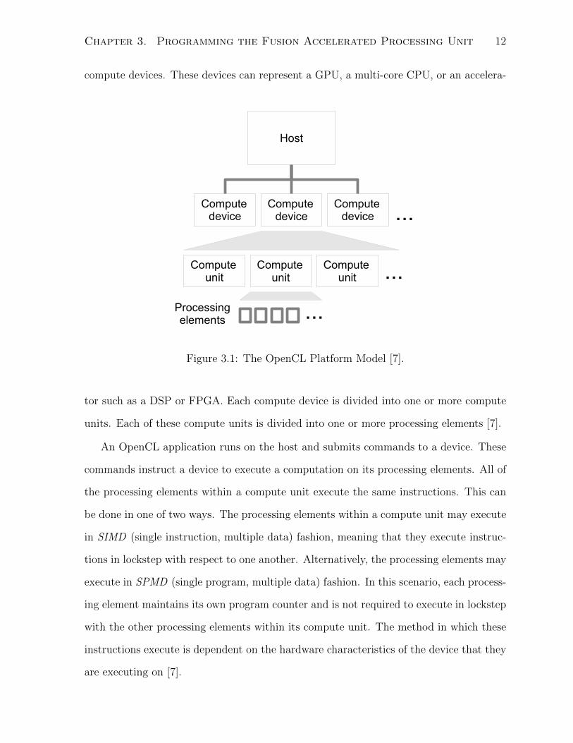
Figure 3.1: The OpenCL Platform Model [7].
tor such as a DSP or FPGA. Each compute device is divided into one or more compute
units. Each of these compute units is divided into one or more processing elements [7].
An OpenCL application runs on the host and submits commands to a device. These
commands instruct a device to execute a computation on its processing elements. All of
the processing elements within a compute unit execute the same instructions. This can
be done in one of two ways. The processing elements within a compute unit may execute
in SIMD (single instruction, multiple data) fashion, meaning that they execute instruc-
tions in lockstep with respect to one another. Alternatively, the processing elements may
execute in SPMD (single program, multiple data) fashion. In this scenario, each process-
ing element maintains its own program counter and is not required to execute in lockstep
with the other processing elements within its compute unit. The method in which these
instructions execute is dependent on the hardware characteristics of the device that they
are executing on [7].
Chapter 3. Programming the Fusion Accelerated Processing Unit 13
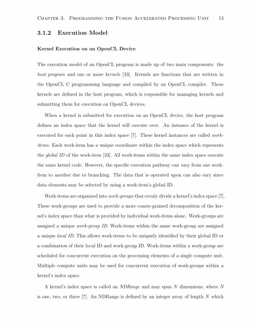
3.1.2 Execution Model
Kernel Execution on an OpenCL Device
The execution model of an OpenCL program is made up of two main components: the
host program and one or more kernels [33]. Kernels are functions that are written in
the OpenCL C programming language and compiled by an OpenCL compiler. These
kernels are defined in the host program, which is responsible for managing kernels and
submitting them for execution on OpenCL devices.
When a kernel is submitted for execution on an OpenCL device, the host program
defines an index space that the kernel will execute over. An instance of the kernel is
executed for each point in this index space [7]. These kernel instances are called work-
items. Each work-item has a unique coordinate within the index space which represents
the global ID of the work-item [33]. All work-items within the same index space execute
the same kernel code. However, the specific execution pathway can vary from one work-
item to another due to branching. The data that is operated upon can also vary since
data elements may be selected by using a work-item’s global ID.
Work-items are organized into work-groups that evenly divide a kernel’s index space [7].
These work-groups are used to provide a more coarse-grained decomposition of the ker-
nel’s index space than what is provided by individual work-items alone. Work-groups are
assigned a unique work-group ID. Work-items within the same work-group are assigned
a unique local ID. This allows work-items to be uniquely identified by their global ID or
a combination of their local ID and work-group ID. Work-items within a work-group are
scheduled for concurrent execution on the processing elements of a single compute unit.
Multiple compute units may be used for concurrent execution of work-groups within a
kernel’s index space.
A kernel’s index space is called an NDRange and may span N dimensions, where N
is one, two, or three [7]. An NDRange is defined by an integer array of length N which
Chapter 3. Programming the Fusion Accelerated Processing Unit 14
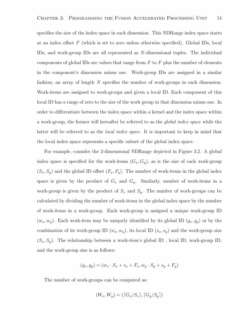
specifies the size of the index space in each dimension. This NDRange index space starts
at an index offset F (which is set to zero unless otherwise specified). Global IDs, local
IDs, and work-group IDs are all represented as N -dimensional tuples. The individual
components of global IDs are values that range from F to F plus the number of elements
in the component’s dimension minus one. Work-group IDs are assigned in a similar
fashion; an array of length N specifies the number of work-groups in each dimension.
Work-items are assigned to work-groups and given a local ID. Each component of this
local ID has a range of zero to the size of the work group in that dimension minus one. In
order to differentiate between the index space within a kernel and the index space within
a work-group, the former will hereafter be referred to as the global index space while the
latter will be referred to as the local index space. It is important to keep in mind that
the local index space represents a specific subset of the global index space.
For example, consider the 2-dimensional NDRange depicted in Figure 3.2. A global
index space is specified for the work-items (Gx, Gy), as is the size of each work-group
(Sx, Sy) and the global ID offset (Fx, Fy). The number of work-items in the global index
space is given by the product of Gx and Gy. Similarly, number of work-items in a
work-group is given by the product of Sx and Sy. The number of work-groups can be
calculated by dividing the number of work-items in the global index space by the number
of work-items in a work-group. Each work-group is assigned a unique work-group ID
(wx, wy). Each work-item may be uniquely identified by its global ID (gx, gy) or by the
combination of its work-group ID (wx, wy), its local ID (sx, sy) and the work-group size
(Sx, Sy). The relationship between a work-item’s global ID , local ID, work-group ID,
and the work-group size is as follows:
(gx, gy) = (wx · Sx + sx + Fx, wy · Sy + sy + Fy)
The number of work-groups can be computed as:
(Wx,Wy) = (dGx/Sxe, dGy/Sye)

Chapter 3. Programming the Fusion Accelerated Processing Unit 15
7.6cm
8.1
cm3cm
3cm
work-item
(wx·S
x+s
x+F
x, w
y·S
y+s
y+F
y)
(sx, s
y) = (0, 0)
...
NDRange size Gy
NDRange size Gx
work-item
(wx·S
x+s
x+F
x, w
y·S
y+s
y+F
y)
(sx, s
y) = (S
x-1, 0)
work-item
(wx·S
x+s
x+F
x, w
y·S
y+s
y+F
y)
(sx, s
y) = (0, S
y-1)
work-item
(wx·S
x+s
x+F
x, w
y·S
y+s
y+F
y)
(sx, s
y) = (S
x-1, S
y-1)
...
... ...
...
work-group size Sx
work-group size Sy
work-group (wx, w
y)
Figure 3.2: An example of an NDRange index space showing work-items, work-groups,and their relationship to global IDs, local IDs, and work-group IDs [7].
where dxe denotes the ceiling function of x. The ceiling function of x is defined as:
dxe = max{m ∈ Z | m ≤ x}
where x and m are real numbers and Z is the set of integers.
The work-group ID of a work-item can be computed as:
(wx, wy) =((gx − sx − Fx)/Sx, (gy − sy − Fy)/Sy
)
Chapter 3. Programming the Fusion Accelerated Processing Unit 16
Context and Command Queues
While kernels are executed on OpenCL devices, the host is responsible for the man-
agement of these kernels and devices [33]. The host does this by defining one or more
contexts within the OpenCL application. The Khronos group defines a context in terms
of the resources it provides [7]:
• Devices: The collection of OpenCL devices to be used by the host.
• Kernels: The OpenCL functions that run on OpenCL devices.
• Program Objects: The program source and executable that implement the ker-
nels.
• Memory Objects: A region of global memory that is visible to the host and the
OpenCL devices. Global memory is described in detail in Section 3.1.3.
The host program uses the OpenCL API to create and manage contexts. Once a
context is created, the host creates one or more command-queues per device. Command-
queues exist within a context, are associated with a particular OpenCL device, and are
used to coordinate execution of commands on the devices. The host places commands
into command-queues, which are then scheduled onto the devices within a context. There
are three types of commands which may be scheduled onto an OpenCL device [7]. Kernel
execution commands execute a kernel on the processing elements of a device. Memory
commands transfer data to, from, or between memory objects. Memory commands may
also map memory objects to the host address space or unmap memory objects from
the host address space. Synchronization commands constrain the order of execution of
commands.
The host code is only responsible for adding commands to a command-queue. It is
the responsibility of the command-queue and underlying OpenCL API implementation
to schedule commands for execution on a device. When a command queue is created, it

Chapter 3. Programming the Fusion Accelerated Processing Unit 17
is designated for either in-order execution or out-of-order execution. When a command-
queue is designated for in-order execution, it means that commands are executed on a
device in the order that they appear in the command queue. In other words, a command
cannot begin execution until all prior commands on the queue have completed. This
serializes the execution order of commands in a queue. When a command-queue is
designated for out-of-order execution, commands in the queue may be executed in any
order. If any particular ordering is desired, it must be enforced by the programmer
through explicit synchronization commands.
Whenever a kernel execution command or a memory command is submitted to a
queue, a corresponding event object is generated. These event objects are used to track
the execution status of a command. Event objects may indicate that their corresponding
command is in one of the following states [7]:
• Queued: The command has been enqueued in a command queue.
• Submitted: The command has been successfully submitted by the host to the
device.
• Running: The device has started executing the command.
• Complete: The command has successfully completed execution.
• Error: An error has occurred. An error code representing the exact error is re-
turned.
When adding a command to a command-queue, it is possible to specify a dependency
list of events that the command is dependent upon. When this happens, all of the events
in the dependency list must be complete before the command will begin to run. This
approach may be used to control the order of execution between commands. It is also
possible to query the status of an event from the host to coordinate execution between
the host and a device.
Chapter 3. Programming the Fusion Accelerated Processing Unit 18
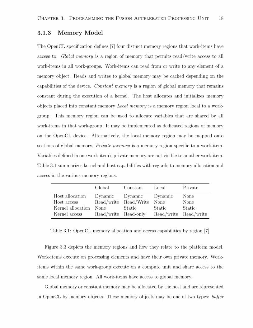
3.1.3 Memory Model
The OpenCL specification defines [7] four distinct memory regions that work-items have
access to. Global memory is a region of memory that permits read/write access to all
work-items in all work-groups. Work-items can read from or write to any element of a
memory object. Reads and writes to global memory may be cached depending on the
capabilities of the device. Constant memory is a region of global memory that remains
constant during the execution of a kernel. The host allocates and initializes memory
objects placed into constant memory Local memory is a memory region local to a work-
group. This memory region can be used to allocate variables that are shared by all
work-items in that work-group. It may be implemented as dedicated regions of memory
on the OpenCL device. Alternatively, the local memory region may be mapped onto
sections of global memory. Private memory is a memory region specific to a work-item.
Variables defined in one work-item’s private memory are not visible to another work-item.
Table 3.1 summarizes kernel and host capabilities with regards to memory allocation and
access in the various memory regions.
Global Constant Local Private
Host allocation Dynamic Dynamic Dynamic NoneHost access Read/write Read/Write None NoneKernel allocation None Static Static StaticKernel access Read/write Read-only Read/write Read/write
Table 3.1: OpenCL memory allocation and access capabilities by region [7].
Figure 3.3 depicts the memory regions and how they relate to the platform model.
Work-items execute on processing elements and have their own private memory. Work-
items within the same work-group execute on a compute unit and share access to the
same local memory region. All work-items have access to global memory.
Global memory or constant memory may be allocated by the host and are represented
in OpenCL by memory objects. These memory objects may be one of two types: buffer
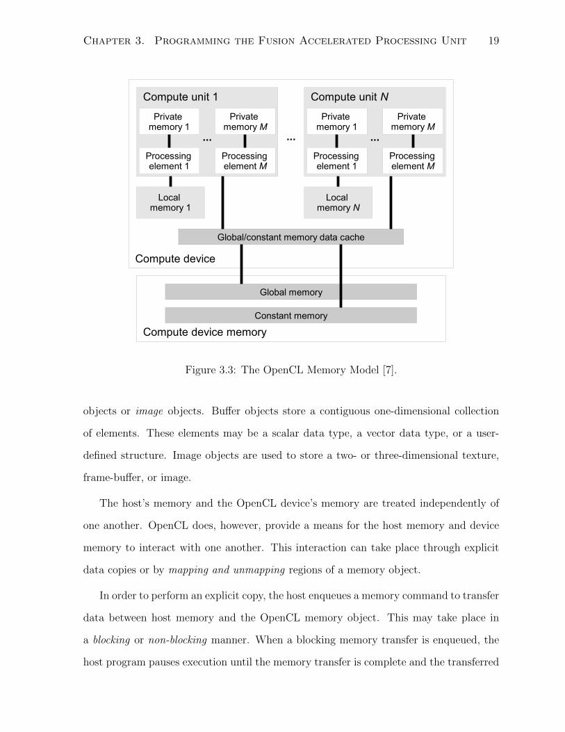
Chapter 3. Programming the Fusion Accelerated Processing Unit 19
Compute device
Compute unit 1
Private memory 1
Processing element 1
...
Private memory M
Processing element M
Compute unit N
Private memory 1
Processing element 1
...
Private memory M
Processing element M
...
Local memory 1
Global/constant memory data cache
Compute device memory
Global memory
Constant memory
Local memory N
Figure 3.3: The OpenCL Memory Model [7].
objects or image objects. Buffer objects store a contiguous one-dimensional collection
of elements. These elements may be a scalar data type, a vector data type, or a user-
defined structure. Image objects are used to store a two- or three-dimensional texture,
frame-buffer, or image.
The host’s memory and the OpenCL device’s memory are treated independently of
one another. OpenCL does, however, provide a means for the host memory and device
memory to interact with one another. This interaction can take place through explicit
data copies or by mapping and unmapping regions of a memory object.
In order to perform an explicit copy, the host enqueues a memory command to transfer
data between host memory and the OpenCL memory object. This may take place in
a blocking or non-blocking manner. When a blocking memory transfer is enqueued, the
host program pauses execution until the memory transfer is complete and the transferred

Chapter 3. Programming the Fusion Accelerated Processing Unit 20
data is safe to use. When a non-blocking memory transfer is enqueued, the host program
continues execution immediately and the memory transfer takes place asynchronously in
the background.
The host may also map and unmap regions of memory objects into its address space.
When a region of memory is mapped into an address space, a virtual address is created
within that address space that can be used to access the mapped region of memory. This
virtual address may map to either a physical address that can be directly resolved, or it
may map to another virtual address that is resolvable by some external device [22].
Once a memory object map is completed, the host is given a pointer to the mapped
region of the memory object. The host is then able to use this pointer to read and write
to this memory region. Once the host has completed its memory accesses to this region,
it unmaps the region.
It is important to note that the OpenCL specification does not define the following
behaviour with regards to mapping and unmapping:
• Accessing a region of a memory object from a device kernel while any portion of
that memory object is mapped to the host.
• Using the pointer returned from a previous map operation to access a previously
mapped memory object region after that memory region has been unmapped from
the host.
In other words, the OpenCL specification only defines behaviour for host accesses to
mapped memory objects and device accesses to unmapped memory objects. It does not
define any scenario where the host and device may access regions of the same memory
object simultaneously.
Chapter 3. Programming the Fusion Accelerated Processing Unit 21
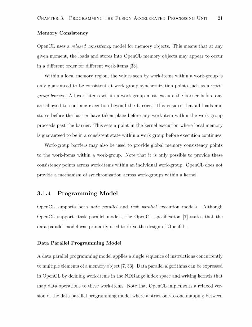
Memory Consistency
OpenCL uses a relaxed consistency model for memory objects. This means that at any
given moment, the loads and stores into OpenCL memory objects may appear to occur
in a different order for different work-items [33].
Within a local memory region, the values seen by work-items within a work-group is
only guaranteed to be consistent at work-group synchronization points such as a work-
group barrier. All work-items within a work-group must execute the barrier before any
are allowed to continue execution beyond the barrier. This ensures that all loads and
stores before the barrier have taken place before any work-item within the work-group
proceeds past the barrier. This sets a point in the kernel execution where local memory
is guaranteed to be in a consistent state within a work group before execution continues.
Work-group barriers may also be used to provide global memory consistency points
to the work-items within a work-group. Note that it is only possible to provide these
consistency points across work-items within an individual work-group. OpenCL does not
provide a mechanism of synchronization across work-groups within a kernel.
3.1.4 Programming Model
OpenCL supports both data parallel and task parallel execution models. Although
OpenCL supports task parallel models, the OpenCL specification [7] states that the
data parallel model was primarily used to drive the design of OpenCL.
Data Parallel Programming Model
A data parallel programming model applies a single sequence of instructions concurrently
to multiple elements of a memory object [7, 33]. Data parallel algorithms can be expressed
in OpenCL by defining work-items in the NDRange index space and writing kernels that
map data operations to these work-items. Note that OpenCL implements a relaxed ver-
sion of the data parallel programming model where a strict one-to-one mapping between
Chapter 3. Programming the Fusion Accelerated Processing Unit 22
work-items and data is not required.
OpenCL provides a hierarchical data parallel programming model. This is achieved by
providing data parallelism from multiple work-items within a work group and data par-
allelism from multiple work-groups within an index space. This hierarchical subdivision
may be specified explicitly or implicitly. In the explicit case, the programmer specifies
the total number of work-items as well as the number of work-items per work-group. In
the implicit case, the programmer only specifies the total number of work-items and the
OpenCL implementation divides them into work-groups.
Task Parallel Programming Model
OpenCL defines a task programming model in which a single instance of a kernel is
executed regardless of the NDRange index space [7]. Under this model, parallelism may
be expressed by performing vector operations over vector data types. Parallelism may
also be expressed by using event dependencies in combination with an out-of-order queue
to execute multiple kernels simultaneously.
3.2 OpenCL on the AMD Fusion APU
The AMD Fusion’s on-die CPU and GPU are both programmable in OpenCL. This is
possible through the use of the AMD Accelerated Parallel Processing SDK, also known
as the AMD APP SDK [2]. The AMD APP SDK provides the necessary tools, libraries,
and environment to develop and build OpenCL applications for AMD CPUs and GPUs.
In addition to using OpenCL, it is also possible to program the CPU in common pro-
gramming languages that support compilation for x86 processors, such as C and C++.
Chapter 3. Programming the Fusion Accelerated Processing Unit 23
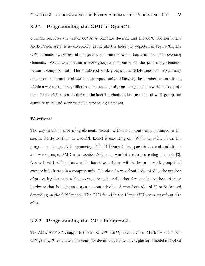
3.2.1 Programming the GPU in OpenCL
OpenCL supports the use of GPUs as compute devices, and the GPU portion of the
AMD Fusion APU is no exception. Much like the hierarchy depicted in Figure 3.1, the
GPU is made up of several compute units, each of which has a number of processing
elements. Work-items within a work-group are executed on the processing elements
within a compute unit. The number of work-groups in an NDRange index space may
differ from the number of available compute units. Likewise, the number of work-items
within a work-group may differ from the number of processing elements within a compute
unit. The GPU uses a hardware scheduler to schedule the execution of work-groups on
compute units and work-items on processing elements.
Wavefronts
The way in which processing elements execute within a compute unit is unique to the
specific hardware that an OpenCL kernel is executing on. While OpenCL allows the
programmer to specify the geometry of the NDRange index space in terms of work-items
and work-groups, AMD uses wavefronts to map work-items to processing elements [3].
A wavefront is defined as a collection of work-items within the same work-group that
execute in lock-step in a compute unit. The size of a wavefront is dictated by the number
of processing elements within a compute unit, and is therefore specific to the particular
hardware that is being used as a compute device. A wavefront size of 32 or 64 is used
depending on the GPU model. The GPU found in the Llano APU uses a wavefront size
of 64.
3.2.2 Programming the CPU in OpenCL
The AMD APP SDK supports the use of CPUs as OpenCL devices. Much like the on-die
GPU, the CPU is treated as a compute device and the OpenCL platform model is applied
Chapter 3. Programming the Fusion Accelerated Processing Unit 24
to it. Each CPU core is treated as a compute unit made up of one processing element.
As a result, a wavefront size of one is used when treating the CPU as an OpenCL device.
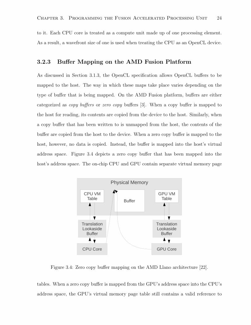
3.2.3 Buffer Mapping on the AMD Fusion Platform
As discussed in Section 3.1.3, the OpenCL specification allows OpenCL buffers to be
mapped to the host. The way in which these maps take place varies depending on the
type of buffer that is being mapped. On the AMD Fusion platform, buffers are either
categorized as copy buffers or zero copy buffers [3]. When a copy buffer is mapped to
the host for reading, its contents are copied from the device to the host. Similarly, when
a copy buffer that has been written to is unmapped from the host, the contents of the
buffer are copied from the host to the device. When a zero copy buffer is mapped to the
host, however, no data is copied. Instead, the buffer is mapped into the host’s virtual
address space. Figure 3.4 depicts a zero copy buffer that has been mapped into the
host’s address space. The on-chip CPU and GPU contain separate virtual memory page
Physical Memory
CPU VM Table Buffer
Translation Lookaside
Buffer
CPU Core
GPU VM Table
Translation Lookaside
Buffer
GPU Core
Figure 3.4: Zero copy buffer mapping on the AMD Llano architecture [22].
tables. When a zero copy buffer is mapped from the GPU’s address space into the CPU’s
address space, the GPU’s virtual memory page table still contains a valid reference to
Chapter 3. Programming the Fusion Accelerated Processing Unit 25
the buffer’s location in physical memory. It should be noted, however, that accessing a
mapped buffer in a device kernel is undefined as per the OpenCL specification [7]. Once a
zero copy buffer is mapped, the host is able to read from and write to this buffer directly.
When the zero copy buffer is unmapped, no data is copied from the host to device.
Chapter 4
Radix Sort
In this chapter we provide an overview of radix sort. We begin by detailing the algorithmic
steps of the sequential version. We then describe the parallel radix sort algorithm as
presented by Satish et al. [35, 36].
4.1 Sequential Algorithm Overview
Coreman et al. [24] classify sorting algorithms into one of two categories: comparison
sorts and non-comparison sorts. A sorting algorithm is classified as a comparison sort if
only value comparisons between elements are used to determine the order of the resulting
output dataset. Radix sort is a sorting algorithm that does not meet this criteria. As
such, it is classified as a non-comparison sort.
Radix sort operates on values that are encoded using positional notation. When a
value x is encoded using positional notation, it is represented using a sequence of d
coefficients (or digits) ci of an infinite power series expansion with a base (or radix ) r as
follows [38]:
x =∞∑
i=−∞
ci · ri = · · ·+ c2 · r2 + c1 · r1 + c0 · r0 + c−1 · r−1 + c−2 · r−2 + · · · (4.1)
For example, consider the unsigned decimal number x = 365. As it is printed in this
26
Chapter 4. Radix Sort 27
document, the number 365 is encoded using positional notation with radix r = 10. It is
represented using d = 3 digits, the coefficients of which are c2 = 3, c1 = 6, c0 = 5. All
other ci coefficients are set to zero. Substituting these values into (4.1) yields:
x =∞∑
i=−∞
ci · ri = · · ·+ 0 · 103 + 3 · 102 + 6 · 101 + 5 · 100 + 0 · 10−1 + · · ·
= 300 + 60 + 5
= 365
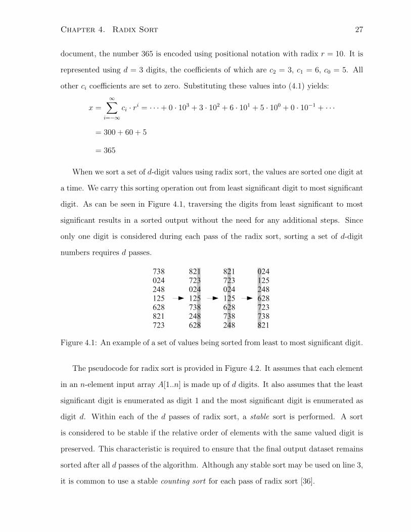
When we sort a set of d-digit values using radix sort, the values are sorted one digit at
a time. We carry this sorting operation out from least significant digit to most significant
digit. As can be seen in Figure 4.1, traversing the digits from least significant to most
significant results in a sorted output without the need for any additional steps. Since
only one digit is considered during each pass of the radix sort, sorting a set of d-digit
numbers requires d passes.
738024248125628821723
821723024125738248628
821723024125628738248
024125248628723738821
Figure 4.1: An example of a set of values being sorted from least to most significant digit.
The pseudocode for radix sort is provided in Figure 4.2. It assumes that each element
in an n-element input array A[1..n] is made up of d digits. It also assumes that the least
significant digit is enumerated as digit 1 and the most significant digit is enumerated as
digit d. Within each of the d passes of radix sort, a stable sort is performed. A sort
is considered to be stable if the relative order of elements with the same valued digit is
preserved. This characteristic is required to ensure that the final output dataset remains
sorted after all d passes of the algorithm. Although any stable sort may be used on line 3,
it is common to use a stable counting sort for each pass of radix sort [36].
Chapter 4. Radix Sort 28
1: function RadixSort(A, d)
2: for currentDigit ← 1 to d do
3: A← CountingSort(A, currentDigit, r);
4: end for
5: end function
Figure 4.2: Pseudocode representation of the sequential version of radix sort.
Counting sort is a non-comparison sort that assumes each of its n input elements
contains an integer value between 0 and k [24]. For each element x in an unsorted input
array A, counting sort determines the number of elements with a value less than x. This
value is then used to place x in the appropriate output position. For example, if there are
12 elements with a value less than x, then it follows that x should be placed in position
13. This description is inadequate, however, in the case that there are several elements
in A that contain the same value. To address this inadequacy we modify our description
of counting sort as follows: for each element x in an unsorted input array A, counting
sort determines the number of elements with a value less than x in A and the number
of elements with a value equal to x that occur before x in A. For example, if there are
12 elements with a value less than x and 2 elements with a value equal to x that occur
before x in A, then 12 + 2 = 14 elements should be placed before x and x should be
placed at position 15. This modification ensures that the counting sort is stable since
the order of equal valued elements is maintained.
The pseudocode for the counting sort that is used by radix sort is provided in Fig-
ure 4.3. It assumes that each element in an n-element input array A[1..n] is made up of
d digits, each of which is in the range 0 to k inclusive. The algorithm returns a sorted
output array B[1..n] and uses intermediate arrays counters [0..k] and countersSum[0..k].
We begin by setting k = r − 1 where r represents the radix that is being used. We then
execute the first step in the counting sort algorithm, which is called the histogram step.
Chapter 4. Radix Sort 29
1: function CountingSort(A, currentDigit, r)
2: k ← r − 1;
3: Histogram(A, counters, k, currentDigit);
4: Rank(counters, countersSum, k);
5: Scatter(A, B, countersSum, k, currentDigit);
6: return B ;
7: end function
Figure 4.3: Pseudocode representation of the sequential version of counting sort.
The pseudocode for the histogram step is provided in Figure 4.4 The histogram step
1: function Histogram(A, counters, k, currentDigit)
2: for i← 0 to k do
3: counters [i ]← 0;
4: end for
5: . All elements of counters are now initialized to zero.
6: for i← 1 to length[A] do
7: digitVal ← CalcDigitValue(A[i], currentDigit);
8: counters [digitVal ]← counters [digitVal ] + 1;
9: end for
10: . counters [i ] now contains the number of elements equal to i.
11: end function
Figure 4.4: Pseudocode representation of the histogram step in the sequential version ofcounting sort.
generates a histogram of the values between 0 and k that are taken on by the current
digit of each element in A. We begin the histogram step by initializing the contents of
counters to zero. We traverse each element in A and store the value of the current digit
that we are sorting on in digitVal. We then increment the counters element at index
digitVal. Once this is complete for all elements in A, the i th element of counters contains
the number of elements in A that have a current digit value equal to i.
Chapter 4. Radix Sort 30
After completing the histogram step, the counting sort pseudocode in Figure 4.3
executes the rank step. The rank step is responsible for calculating the output location
in B where we will place the elements in A. The pseudocode for the rank step is provided
in Figure 4.5. The rank step carries out an inclusive prefix sum over counters and stores
1: function Rank(counters, countersSum, k)
2: for i← 1 to k do
3: countersSum[i]← counters [i] + countersSum[i− 1];
4: end for
5: . counters [i ] now contains the number of elements less than or equal to i.
6: end function
Figure 4.5: Pseudocode representation of the rank step in the sequential version of count-ing sort.
the result in countersSum. According to Blelloch [20], a prefix sum, or scan “instruction
for a binary associative operator⊕
, takes a vector of values” X “and returns to each
position of a new equal-length vector, the operator sum of all previous positions in” X.
The prefix sum in Figure 4.5 is said to be inclusive because countersSum[i] contains
the sum of all the values in counters from index 0 up to and including index i. The
following example illustrates the concept of an inclusive prefix sum using the counters
and countersSum buffers:
counters = [ 3 2 1 1 2 3 ]
countersSum = [ 3 5 6 7 9 12 ]
Note that each element in the countersSum buffer is equal to the sum of the elements in
the counters buffer that occur at a lower or equal array index value.
After completing the rank step, the counting sort in Figure 4.3 executes the scatter
step. The scatter step is responsible for placing the contents of A in the correct position
in B. The pseudocode for the scatter step is provided in Figure 4.6. The scatter step
traverses array A backwards and writes each element to the appropriate location in array
Chapter 4. Radix Sort 31
1: function Scatter(A, B, countersSum, k, currentDigit)
2: for i← length[A] downto 1 do
3: digitVal← CalcDigitValue(A[i], currentDigit);
4: outputLocation← countersSum[digitVal ];
5: B[outputLocation]← A[i];
6: countersSum[digitVal ]← countersSum[digitVal ]− 1;
7: end for
8: . All elements in B are now sorted by digit currentDigit.
9: end function
Figure 4.6: Pseudocode representation of the scatter step in the sequential version ofcounting sort.
B. For each element in A, we first isolate the current digit value and store it in digitVal.
We then determine what the output location is based on the prefix sum data in coun-
tersSum that was generated during the rank step. The value of countersSum[digitVal ]
is the index where we should place A[i] in B since countersSum[digitVal ] contains the
number of elements with a current digit value less than or equal to digitVal. We decre-
ment countersSum[digitV al] so that no two elements in A are placed in the same output
location in B. Traversing array A backwards and decrementing countersSum[digitV al]
ensures that the relative order of elements with the same value is maintained. Counting
sort is therefore considered to be a stable sort.
4.2 Parallel Radix Sort Algorithm
Radix sort may be parallelized by dividing the unsorted input array A into T equally
sized tiles. Within each pass of parallel radix sort, we assign each tile At in A to a
work-group and carry out a modified counting sort. Much like in the sequential version
of radix sort, this counting sort consists of histogram, rank, and scatter steps. Each of
these steps is implemented in its own OpenCL kernel.
Chapter 4. Radix Sort 32
During a given pass of radix sort, the current digit that is being sorted on may take on
integer values between 0 and k = r−1 where r represents the radix value. The histogram
in the sequential version of radix sort described in Section 4.1 is responsible for generating
a histogram buffer counters of current digit values within A. The purpose of this is to
generate a buffer counters where the i th element of counters contains the number of
elements in A that have a current digit value equal to i. Similarly, the histogram in
the parallel version of radix sort is responsible for generating T histograms in a buffer
counters, one for each of the T tiles in A. For each histogram tile counterst in counters,
the i th element of counterst contains the number of elements in At that have a current
digit value equal to i.
Once the counters buffer is generated, the rank kernel may begin execution. The rank
kernel in the sequential version of radix sort is responsible for carrying out a prefix sum
over counters as described in Section 4.1. This generates a buffer countersSum where
each element in countersSum is equal to the sum of the elements in the counters buffer
that occur at a lower or equal array index value. The rank kernel in the parallel version
of radix sort operates in a similar manner, however it must account for the fact that
there are T tiles. In order to determine the correct position to place elements, we must
determine the number of elements that have a lower current digit value in all T tiles of
A. In order for the sort to remain stable, we must also determine the number of elements
that have an equal current digit value in earlier tiles of A. This is accomplished by
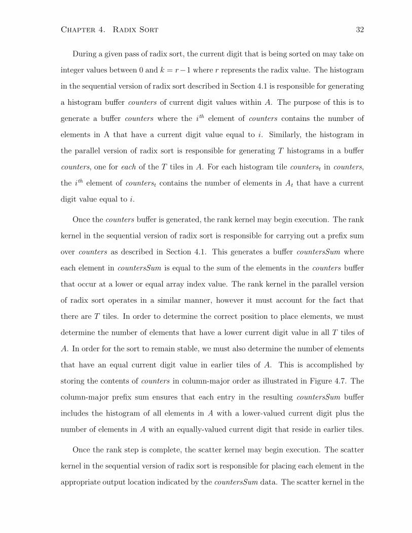
storing the contents of counters in column-major order as illustrated in Figure 4.7. The
column-major prefix sum ensures that each entry in the resulting countersSum buffer
includes the histogram of all elements in A with a lower-valued current digit plus the
number of elements in A with an equally-valued current digit that reside in earlier tiles.
Once the rank step is complete, the scatter kernel may begin execution. The scatter
kernel in the sequential version of radix sort is responsible for placing each element in the
appropriate output location indicated by the countersSum data. The scatter kernel in the
Chapter 4. Radix Sort 33
0
1
2
T-1
0 1 2 . . . k
Column-majorstorage for prefix sum
Histogram tiles
Digit values
Counters buffer
Figure 4.7: The counters buffer is stored in column-major order for the prefix sumoperation [36].
parallel version is responsible for the same task. Each work-item is assigned an element to
place in the correct output position. There are two problems in this approach. The first
is that GPU performance of scattered writes is slower than that of streaming writes. This
is because when all work-items within a wavefront access consecutive memory addresses,
the GPU is able to coalesce these memory accesses into a single transaction [3]. Coalesced
memory accesses provide higher data transfer rates than uncoalesced memory accesses.
The second problem is that elements with the same current digit value may be located
anywhere within a work-group’s unsorted input tile At . Work-items are not aware of
how many elements with the same current digit value should be placed before or after
the work-item’s assigned element. Satish et al. [36] address both of these problems by
introducing a new step at the beginning of each parallel radix sort pass that locally sorts
the data within each tile.
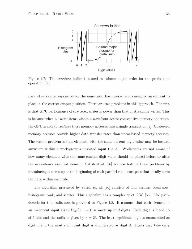
The algorithm presented by Satish et, al. [36] consists of four kernels: local sort,
histogram, rank, and scatter. This algorithm has a complexity of O(n) [36]. The pseu-
docode for this radix sort is provided in Figure 4.8. It assumes that each element in
an n-element input array keys [0..n − 1] is made up of d digits. Each digit is made up
of b bits and the radix is given by r = 2b. The least significant digit is enumerated as
digit 1 and the most significant digit is enumerated as digit d. Digits may take on a
Chapter 4. Radix Sort 34
value between 0 and r − 1. The algorithm uses intermediate arrays tempKeys [0..n− 1],
tileOffsets [0..m− 1], counters [0..m− 1] and countersSum[0..m− 1] where m = r ·T . The
variable startBit contains the starting bit of the current digit in each pass.
1: function RadixSort(keys, d)
2: for currentDigit ← 1 to d do
3: LocalSort(out:tempKeys, in:keys, in:startBit, in:b);
4: Histogram(out:tileOffsets, out:counters, in:tempKeys,
in:startBit, in:b, in:r, in:tileSize, in:t);
5: Rank(out:countersSum, in:counters, in:m);
6: Scatter(out:keys, in:tempKeys, in:tileOffsets, in:countersSum,
in:startBit, in:b, in:r, in:tileSize, in:t);
7: end for
8: end function
Figure 4.8: Pseudocode representation of the parallel version of radix sort.
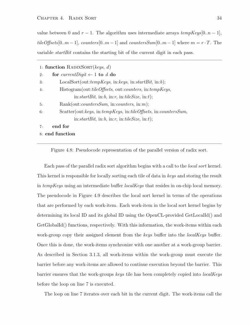
Each pass of the parallel radix sort algorithm begins with a call to the local sort kernel.
This kernel is responsible for locally sorting each tile of data in keys and storing the result
in tempKeys using an intermediate buffer localKeys that resides in on-chip local memory.
The pseudocode in Figure 4.9 describes the local sort kernel in terms of the operations
that are performed by each work-item. Each work-item in the local sort kernel begins by
determining its local ID and its global ID using the OpenCL-provided GetLocalId() and
GetGlobalId() functions, respectively. With this information, the work-items within each
work-group copy their assigned element from the keys buffer into the localKeys buffer.
Once this is done, the work-items synchronize with one another at a work-group barrier.
As described in Section 3.1.3, all work-items within the work-group must execute the
barrier before any work-items are allowed to continue execution beyond the barrier. This
barrier ensures that the work-groups keys tile has been completely copied into localKeys
before the loop on line 7 is executed.
The loop on line 7 iterates over each bit in the current digit. The work-items call the
Chapter 4. Radix Sort 35
1: function LocalSort(tempKeys , keys , startBit, b)
2: localId ← GetLocalId();
3: globalId ← GetGlobalId();
4: localKeys [localId ]← keys [globalId ];
5: WorkGroupBarrier();
6: . This work-group’s keys tile has now been copied to the on-chip localKeys buffer.
7: for currentBit ← startBit to b do
8: Split(localKeys, currentBit);
9: WorkGroupBarrier();
10: . localKeys has now been sorted by the currentBit bit.
11: end for
12: . localKeys has now been sorted by all bits in the current digit.
13: tempKeys [globalId ]← localKeys [localId ];
14: WorkGroupBarrier();
15: . This work-group’s sorted localKeys data has been copied to the tempKeys buffer.
16: end function
Figure 4.9: Pseudocode representation of the parallel local sort kernel.
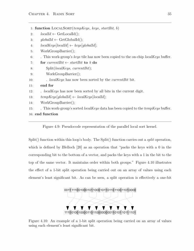
Split() function within this loop’s body. The Split() function carries out a split operation,
which is defined by Blelloch [20] as an operation that “packs the keys with a 0 in the
corresponding bit to the bottom of a vector, and packs the keys with a 1 in the bit to the
top of the same vector. It maintains order within both groups.” Figure 4.10 illustrates
the effect of a 1-bit split operation being carried out on an array of values using each
element’s least significant bit. As can be seen, a split operation is effectively a one-bit
1011011011001101000000111110010001011000
101101101100 11010000001111100100 01011000
Figure 4.10: An example of a 1-bit split operation being carried on an array of valuesusing each element’s least significant bit.
Chapter 4. Radix Sort 36
radix sort operation. Split operations have been efficiently implemented on GPUs by
Harris et al. [28] and are available in GPU data parallel primitive software packages such
as the CUDA Data-Parallel Primitives (CUDPP) library [12].
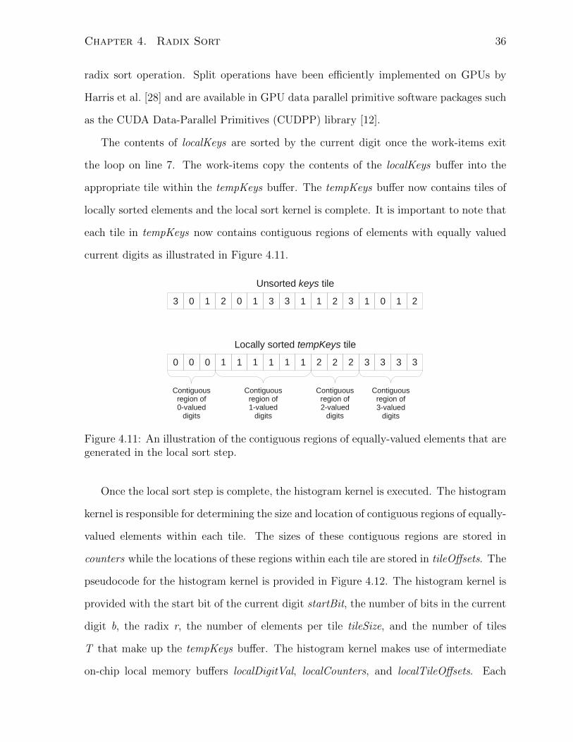
The contents of localKeys are sorted by the current digit once the work-items exit
the loop on line 7. The work-items copy the contents of the localKeys buffer into the
appropriate tile within the tempKeys buffer. The tempKeys buffer now contains tiles of
locally sorted elements and the local sort kernel is complete. It is important to note that
each tile in tempKeys now contains contiguous regions of elements with equally valued
current digits as illustrated in Figure 4.11.
0 0 0 1 1 1 1 1 1 2 2 2 3 3 3 3
0 0 01 11 11 12 2 23 33 3
Unsorted keys tile
Locally sorted tempKeys tile
Contiguous region of0-valued
digits
Contiguous region of1-valued
digits
Contiguous region of2-valued
digits
Contiguous region of3-valued
digits
Figure 4.11: An illustration of the contiguous regions of equally-valued elements that aregenerated in the local sort step.
Once the local sort step is complete, the histogram kernel is executed. The histogram
kernel is responsible for determining the size and location of contiguous regions of equally-
valued elements within each tile. The sizes of these contiguous regions are stored in
counters while the locations of these regions within each tile are stored in tileOffsets. The
pseudocode for the histogram kernel is provided in Figure 4.12. The histogram kernel is
provided with the start bit of the current digit startBit, the number of bits in the current
digit b, the radix r, the number of elements per tile tileSize, and the number of tiles
T that make up the tempKeys buffer. The histogram kernel makes use of intermediate
on-chip local memory buffers localDigitVal, localCounters, and localTileOffsets. Each
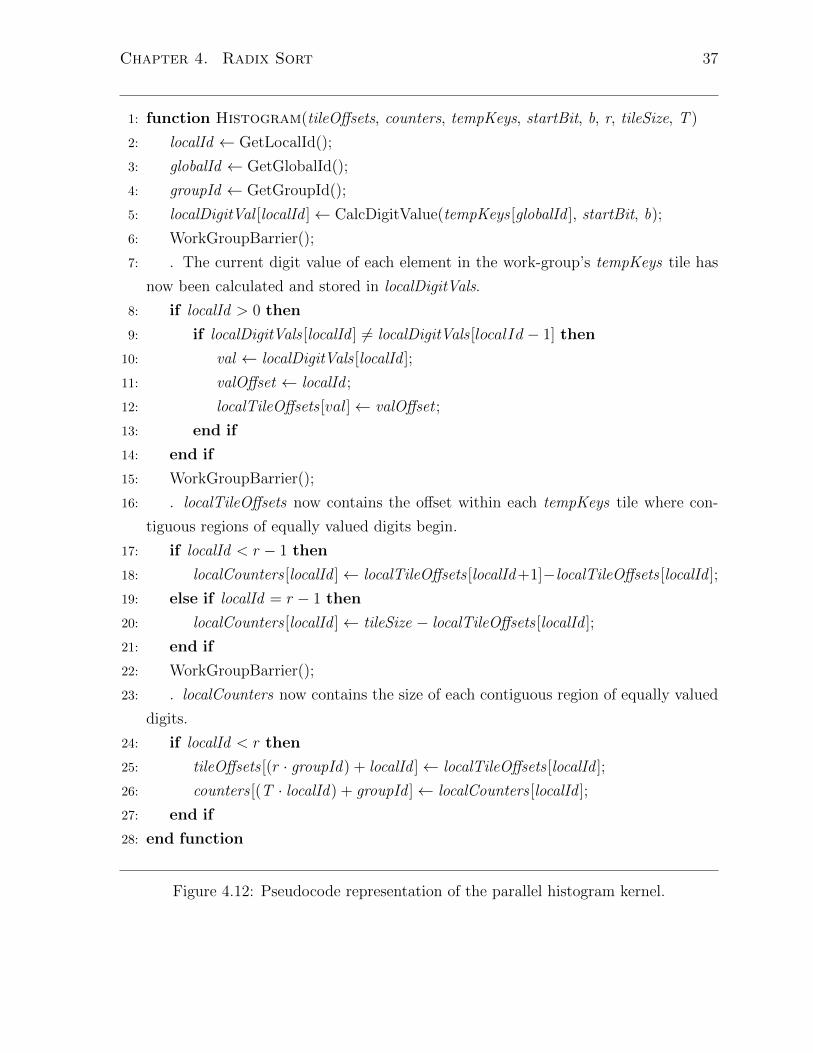
Chapter 4. Radix Sort 37
1: function Histogram(tileOffsets, counters, tempKeys, startBit, b, r, tileSize, T )
2: localId ← GetLocalId();
3: globalId ← GetGlobalId();
4: groupId ← GetGroupId();
5: localDigitVal [localId ]← CalcDigitValue(tempKeys [globalId ], startBit, b);
6: WorkGroupBarrier();
7: . The current digit value of each element in the work-group’s tempKeys tile has
now been calculated and stored in localDigitVals.
8: if localId > 0 then
9: if localDigitVals [localId ] 6= localDigitVals [localId− 1] then
10: val ← localDigitVals [localId ];
11: valOffset ← localId ;
12: localTileOffsets [val]← valOffset ;
13: end if
14: end if
15: WorkGroupBarrier();
16: . localTileOffsets now contains the offset within each tempKeys tile where con-
tiguous regions of equally valued digits begin.
17: if localId < r − 1 then
18: localCounters [localId ]← localTileOffsets [localId +1]−localTileOffsets [localId ];
19: else if localId = r − 1 then
20: localCounters [localId ]← tileSize − localTileOffsets [localId ];
21: end if
22: WorkGroupBarrier();
23: . localCounters now contains the size of each contiguous region of equally valued
digits.
24: if localId < r then
25: tileOffsets [(r · groupId) + localId ]← localTileOffsets [localId ];
26: counters [(T · localId) + groupId ]← localCounters [localId ];
27: end if
28: end function
Figure 4.12: Pseudocode representation of the parallel histogram kernel.
Chapter 4. Radix Sort 38
work-item begins by determining its local ID, global ID, and work-group ID. Each work-
item then calculates the value of its assigned element’s current digit and stores this
value in local memory. Once all work-items within the work-group have populated the
localDigitVals buffer, adjacent elements in the localDigitVals buffer are compared with
one another. Since each tile in tempKeys is locally sorted by the current digit, the
localDigitVals buffer contains r contiguous regions of equally valued elements. If the value
of two adjacent elements in the localDigitVals buffer are not equal, then the boundary
of one such contiguous region has been found. The location where the contiguous region
begins within the tile is recorded in localTileOffsets on line 12. Once localTileOffsets is
populated, taking the difference between adjacent elements in the buffer provides us with
the size of each contiguous region. This value is stored in localCounters. Once this is
complete, the tile offset and counters data is copied from local memory to global memory.
It is important to note that counters now contains the size of each of the aforementioned
contiguous regions. Likewise, tileOffsets now contains the index of each contiguous region
within its tile.
After the histogram step is complete, the rank kernel is executed. Each of the T tiles
in the tempKeys buffer contains up to r contiguous regions of elements with equal current
digit values. The rank kernel is responsible for determining the location where each of
these regions should be placed. The kernel carries out an exclusive parallel-prefix sum of
the counters buffer and stores the result in the countersSum buffer. A prefix sum is said
to be exclusive since countersSum[i ] contains the sum of all the values in counters from
index 0 up to and not including index i. The following example illustrates the concept
of an exclusive prefix sum using the counters and countersSum buffers:
counters = [ 3 2 1 1 2 3 ]
countersSum = [ 0 3 5 6 7 9 ]
Prefix sum operations have been efficiently implemented on GPUs by Harris et al. [28]
and are available in GPU data parallel primitive software packages such as the CUDA
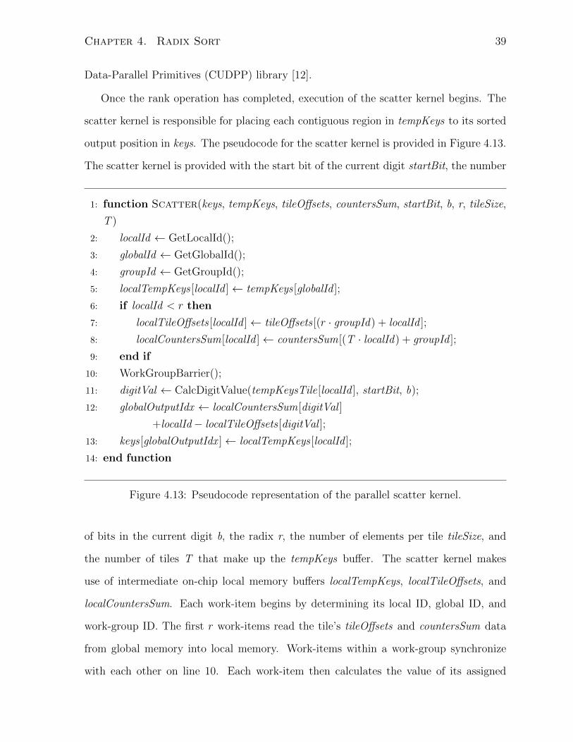
Chapter 4. Radix Sort 39
Data-Parallel Primitives (CUDPP) library [12].
Once the rank operation has completed, execution of the scatter kernel begins. The
scatter kernel is responsible for placing each contiguous region in tempKeys to its sorted
output position in keys. The pseudocode for the scatter kernel is provided in Figure 4.13.
The scatter kernel is provided with the start bit of the current digit startBit, the number
1: function Scatter(keys, tempKeys, tileOffsets, countersSum, startBit, b, r, tileSize,
T )
2: localId ← GetLocalId();
3: globalId ← GetGlobalId();
4: groupId ← GetGroupId();
5: localTempKeys [localId ]← tempKeys [globalId ];
6: if localId < r then
7: localTileOffsets [localId ]← tileOffsets [(r · groupId) + localId ];
8: localCountersSum[localId ]← countersSum[(T · localId) + groupId ];
9: end if
10: WorkGroupBarrier();
11: digitVal ← CalcDigitValue(tempKeysTile[localId ], startBit, b);
12: globalOutputIdx ← localCountersSum[digitVal ]
+localId− localTileOffsets [digitVal ];
13: keys [globalOutputIdx ]← localTempKeys [localId ];
14: end function
Figure 4.13: Pseudocode representation of the parallel scatter kernel.
of bits in the current digit b, the radix r, the number of elements per tile tileSize, and
the number of tiles T that make up the tempKeys buffer. The scatter kernel makes
use of intermediate on-chip local memory buffers localTempKeys, localTileOffsets, and
localCountersSum. Each work-item begins by determining its local ID, global ID, and
work-group ID. The first r work-items read the tile’s tileOffsets and countersSum data
from global memory into local memory. Work-items within a work-group synchronize
with each other on line 10. Each work-item then calculates the value of its assigned

Chapter 4. Radix Sort 40
element’s current digit and stores it in local memory. Work-items calculate the output
location where their respective elements should be placed in the keys buffer. The elements
are copied to the correct position in the keys buffer and the scatter step is complete.
Chapter 5
Fusion Sort
In this chapter we propose utilizing the CPU in order to increase the performance of
radix sort on the AMD Fusion Accelerated Processing Unit and discuss the resulting
challenges that arise. We then present several means of addressing these challenges and
discuss the potential performance implications that are associated with them. We finally
provide an algorithmic overview of three radix sort algorithms which we collectively refer
to as Fusion Sort. Each of these algorithms address these challenges differently.
5.1 Motivation
The parallel NVIDIA algorithm presented by Satish et al. [35, 36] is designed for execution
only on a GPU device. The CPU remains idle during this execution and does not
participate in the sort. Our goal is to allow the CPU to participate in the sort in order to
further increase the performance of radix sort. Several challenges arise when introducing
the CPU as a participant in the sort. These challenges can be addressed in several ways,
each of which has an impact on performance.
The NVIDIA algorithm presented by Satish et al. [35, 36] employs a data parallel
programming model that breaks each kernel’s input into tiles that are processed in parallel
on the GPU. It is intuitive to extend this model in order to achieve parallelism between
41
Chapter 5. Fusion Sort 42
the GPU and the CPU devices. Thus, we elect to use a data parallel programming model
where the input dataset is partitioned between the GPU and CPU devices.
The goal of partitioning the input dataset between the GPU and CPU is to ensure
that each device takes an equal amount of time to carry out its assigned portion of the
algorithm’s computational workload, thereby reducing the overall execution time of the
sort. This partitioning may take place once at the beginning of the algorithm and kept
for the duration of its execution or the partitioning may change at each kernel step. We
refer to the former as static partitioning and the latter as dynamic partitioning.
Static partitioning provides the advantage of allowing for a coarse-grained data shar-
ing model where the amount of communication between the GPU and CPU is relatively
low. Each device can be thought of as the owner of the data that it is reading from or
writing to and little data is transfered between the two devices. Static partitioning may
not, however, be a suitable choice if certain kernel steps perform better on the GPU while
other kernel steps perform better on the CPU. In this case it may be better to repartition
the dataset at each kernel step, which we call dynamic partitioning.
Dynamic partitioning allows the workload and its associated data to be distributed
between the GPU and the CPU at each kernel step. This allows us to eliminate workload
imbalance at a per-kernel granularity, which may increase the overall performance of radix
sort. The disadvantage of dynamic partitioning is that it requires a fine-grained data
sharing model where data is passed back and forth between the CPU and GPU. This
results in a relatively high amount of communication and synchronization between the
devices. It is therefore unclear which partitioning method will result in better radix sort
performance.
The second challenge is identifying the optimal way in which to allocate the memory
buffers used by the algorithm. These buffers may be allocated as either copy buffers or
zero copy buffers, as discussed in Section 3.2.3. If a buffer is allocated as a zero copy
buffer, then we must decide on the memory region in which to allocate it. There are
Chapter 5. Fusion Sort 43
several possible regions in which memory may be allocated, each of which is accessible
at different speeds by the GPU and CPU, as discussed in Section 2.2. We must therefore
decide on how to best allocate data while considering how it will be used in each step of
the sort.
We present three radix sort algorithms that address the aforementioned challenges
in different ways. They each use a different combination of data sharing granularity,
partitioning methods and memory allocation strategies. These algorithms are named
Coarse-Grained, Fine-Grained Static, and Fine-Grained Dynamic.
5.2 Coarse-Grained Algorithm
The Coarse-Grained algorithm uses both devices to independently execute the parallel
radix sort algorithm described in Section 4.2 on the unsorted input data. The pseu-
docode for the complete Coarse-Grained implementation is provided in Figure 5.1. The
CPU’s pseudocode is provided in Figure 5.1a while the GPU’s pseudocode is provided in
Figure 5.1b.
The algorithm begins by copying p% of the unsorted input data to the GPU. This
value p% is the percent of the sorting workload that has been assigned to the GPU and
is referred to as the GPU partition point. Once this data has been copied to the GPU,
the GPU and CPU synchronize with one another on line 2 to ensure that the GPU’s
portion of the unsorted input dataset has been written to the gpuKeys buffer before
the GPU begins executing the parallel radix sort algorithm. Once this synchronization
takes place, the CPU copies the remaining (1 − p)% of the unsorted input data into its
cpuKeys buffer and the two devices simultaneously execute their respective variants of
parallel radix sort. After all passes of the parallel radix sort have been carried out on
both devices, the GPU and CPU again synchronize with one another. At this point
the elements in the cpuKeys buffer and gpuKeys buffer are individually sorted and the

Chapter 5. Fusion Sort 44
1: Write p% of unsorted data to gpuKeys
on the GPU;
2: Sync();
3: Write (1 − p)% of unsorted data to
cpuKeys ;
4: for cpuPass ← 1 to numPasses do
5: LocalSort(cpuKeys,
cpuTempKeys);
6: Histogram(cpuTempKeys,
cpuTileOffsets,
cpuCounters);
7: Rank(cpuCounters,
cpuCountersSum);
8: Scatter(cpuTempKeys,
cpuTileOffsets,
cpuCountersSum,
cpuKeys);
9: end for
10: Sync();
11: Read gpuKeys from GPU;
12: Merge(cpuKeys,
gpuKeys,
mergedKeys);
13: return mergedKeys
(a) CPU pseudocode.
1:
2: Sync();
3:
4: for gpuPass ← 1 to numPasses do
5: LocalSort(gpuKeys,
gpuTempKeys);
6: Histogram(gpuTempKeys,
gpuTileOffsets,
gpuCounters);
7: Rank(gpuCounters,
gpuCountersSum);
8: Scatter(gpuTempKeys,
gpuTileOffsets,
gpuCountersSum,
gpuKeys);
9: end for
10: Sync();
11:
12:
13:
(b) GPU pseudocode.
Figure 5.1: Pseudocode representation of the Coarse-Grained algorithm.
CPU may read the contents of gpuKeys from the GPU. The CPU must then merge the
contents of the gpuKeys buffer with the contents of the cpuKeys buffer. This generates
a single sorted output and completes the Coarse-Grained sort algorithm.
While the same kernel steps are carried out on both the GPU and the CPU, the
details of the implementation vary between devices. When executing on the GPU, the
Chapter 5. Fusion Sort 45
GPU kernel steps closely follow the kernel algorithms described in Section 4.2. The CPU,
however, runs a modified set of kernels that have been optimized for execution on the
CPU.
The Coarse-Grained algorithm addresses the first challenge by using a static partition
point that is set at the beginning of the algorithm. As the algorithm’s name suggests, a
coarse-grained data sharing model is employed; there are relatively few synchronization
points in the algorithm and little data sharing takes place between the GPU and the
CPU. Data is only shared between the GPU and the CPU when the gpuKeys buffer is
written to the GPU at the beginning of the algorithm and when the gpuKeys buffer is
read from GPU at the end of the algorithm. These steps must be carried out regardless
of whether or not the gpuKeys buffer is of zero copy type. As a result, we do not use
zero copy buffers in this algorithm. Each device’s buffers are allocated in the device’s
preferred memory region; the CPU’s buffers are allocated in cached host memory while
the GPU’s buffers are allocated in uncached device-visible host memory.
5.3 Fine-Grained Static Algorithm
The Fine-Grained Static algorithm shares data between the CPU and GPU during each
pass of the sort, thereby utilizing a finer granularity of data sharing than the Coarse-
Grained algorithm. The pseudocode for this algorithm is provided in Figure 5.2. The
CPU’s pseudocode is shown in Figure 5.2a while the GPU’s pseudocode is shown in
Figure 5.2b.
At the beginning of the algorithm, the CPU copies p% of the unsorted input data
into the gpuKeys buffer. The two devices then synchronize and begin execution of the
parallel radix sort algorithm. Each device carries out the local sort step on the data
in its respective keys buffer. This data is written out to the device’s tempKeys buffer.
The histogram step then executes and generates the device’s tileOffsets and counters
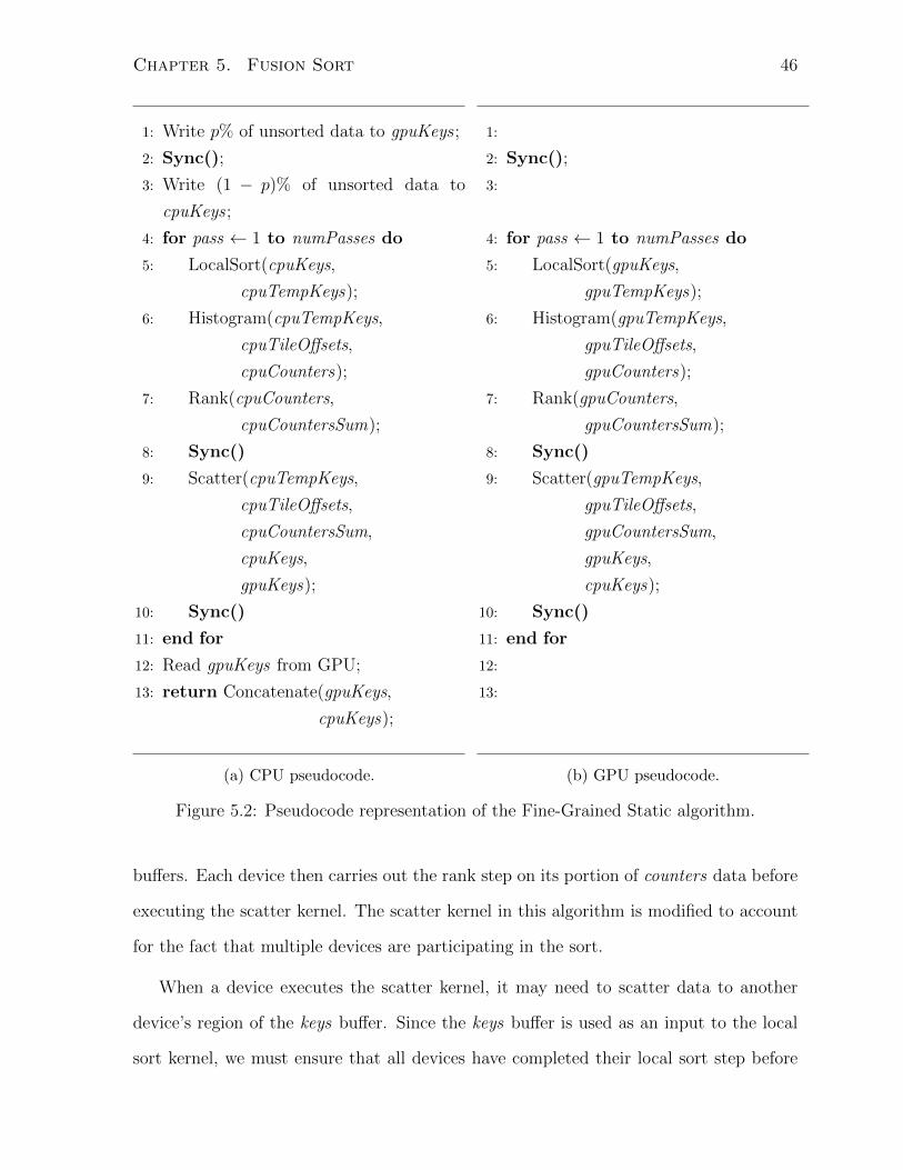
Chapter 5. Fusion Sort 46
1: Write p% of unsorted data to gpuKeys ;
2: Sync();
3: Write (1 − p)% of unsorted data to
cpuKeys ;
4: for pass ← 1 to numPasses do
5: LocalSort(cpuKeys,
cpuTempKeys);
6: Histogram(cpuTempKeys,
cpuTileOffsets,
cpuCounters);
7: Rank(cpuCounters,
cpuCountersSum);
8: Sync()
9: Scatter(cpuTempKeys,
cpuTileOffsets,
cpuCountersSum,
cpuKeys,
gpuKeys);
10: Sync()
11: end for
12: Read gpuKeys from GPU;
13: return Concatenate(gpuKeys,
cpuKeys);
(a) CPU pseudocode.
1:
2: Sync();
3:
4: for pass ← 1 to numPasses do
5: LocalSort(gpuKeys,
gpuTempKeys);
6: Histogram(gpuTempKeys,
gpuTileOffsets,
gpuCounters);
7: Rank(gpuCounters,
gpuCountersSum);
8: Sync()
9: Scatter(gpuTempKeys,
gpuTileOffsets,
gpuCountersSum,
gpuKeys,
cpuKeys);
10: Sync()
11: end for
12:
13:
(b) GPU pseudocode.
Figure 5.2: Pseudocode representation of the Fine-Grained Static algorithm.
buffers. Each device then carries out the rank step on its portion of counters data before
executing the scatter kernel. The scatter kernel in this algorithm is modified to account
for the fact that multiple devices are participating in the sort.
When a device executes the scatter kernel, it may need to scatter data to another
device’s region of the keys buffer. Since the keys buffer is used as an input to the local
sort kernel, we must ensure that all devices have completed their local sort step before

Chapter 5. Fusion Sort 47
executing the scatter kernel. We do this by inserting a synchronization point at line 8.
Likewise, we must ensure that all devices have completed the scatter operation before
beginning execution of the next iteration’s local sort kernel. We ensure this by inserting
another synchronization point at line 10. Once all passes of the sort are complete, the
CPU reads the GPU’s portion of the keys buffer from the GPU. The CPU’s portion of
the keys buffer is concatenated to this and the sort is complete.
The Fine-Grained Static algorithm addresses the challenge of workload partitioning
by choosing a static partition point for the duration of the sort. As its name suggests,
the Fine-Grained Static algorithm uses a fine-grained data sharing model. Several syn-
chronization points take place before and after the scatter kernel during each pass of the
sort. The scatter step shares a large amount of data between the CPU and the GPU as
it moves elements to their sorted locations.
In order to prevent the introduction of extra steps that merge the CPU’s and GPU’s
respective scatter outputs, this algorithm requires that the cpuKeys and gpuKeys buffers
be writable by both devices simultaneously. We therefore must allocate these buffers as
zero copy type. The cpuKeys buffer is allocated in cacheable host memory. This provides
fast CPU write access during the scatter step as well as fast CPU read access during the
local sort step. The GPU is able to write to this memory buffer at reasonable speeds
during the scatter step. The gpuKeys buffer is allocated in uncached device-visible host
memory. This provides fast GPU write access during the scatter step as well as fast
GPU read access during the local sort step. The CPU is able to write to this region at
relatively fast speeds during the scatter step by making use of the available on-chip write
combining buffers.
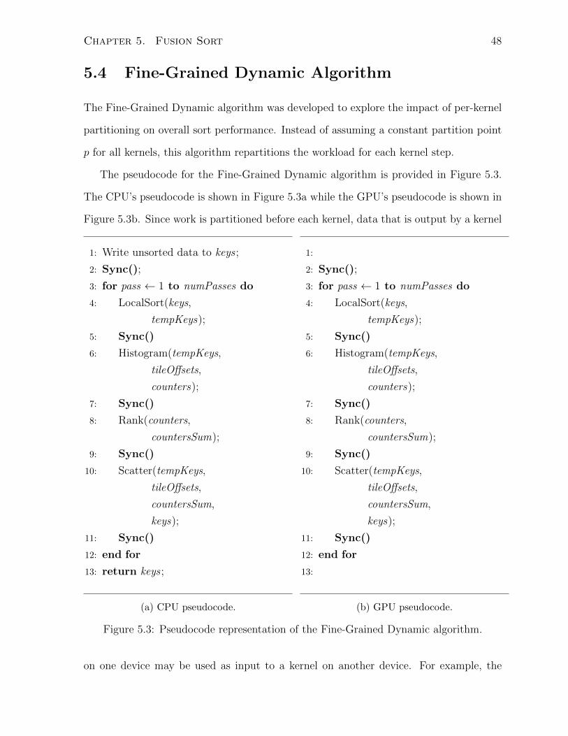
Chapter 5. Fusion Sort 48
5.4 Fine-Grained Dynamic Algorithm
The Fine-Grained Dynamic algorithm was developed to explore the impact of per-kernel
partitioning on overall sort performance. Instead of assuming a constant partition point
p for all kernels, this algorithm repartitions the workload for each kernel step.
The pseudocode for the Fine-Grained Dynamic algorithm is provided in Figure 5.3.
The CPU’s pseudocode is shown in Figure 5.3a while the GPU’s pseudocode is shown in
Figure 5.3b. Since work is partitioned before each kernel, data that is output by a kernel
1: Write unsorted data to keys ;
2: Sync();
3: for pass ← 1 to numPasses do
4: LocalSort(keys,
tempKeys);
5: Sync()
6: Histogram(tempKeys,
tileOffsets,
counters);
7: Sync()
8: Rank(counters,
countersSum);
9: Sync()
10: Scatter(tempKeys,
tileOffsets,
countersSum,
keys);
11: Sync()
12: end for
13: return keys ;
(a) CPU pseudocode.
1:
2: Sync();
3: for pass ← 1 to numPasses do
4: LocalSort(keys,
tempKeys);
5: Sync()
6: Histogram(tempKeys,
tileOffsets,
counters);
7: Sync()
8: Rank(counters,
countersSum);
9: Sync()
10: Scatter(tempKeys,
tileOffsets,
countersSum,
keys);
11: Sync()
12: end for
13:
(b) GPU pseudocode.
Figure 5.3: Pseudocode representation of the Fine-Grained Dynamic algorithm.
on one device may be used as input to a kernel on another device. For example, the
Chapter 5. Fusion Sort 49
output of the local sort kernel on one device may be used as the input to the histogram
or scatter kernels on a different device. Likewise, the tileOffsets data that is generated
on one device may be required in the scatter step of another device. One consequence
of this is that we now require synchronization points between each kernel step as can
be seen on lines 5, 7, 9 and 11. Another consequence is that we can no longer consider
a device to be the owner of the data that it is reading from or writing to. Instead of
dividing a buffer into one region for the CPU and another region for the GPU, the entire
buffer contents must now be visible to both devices during kernel execution. This results
in a relatively high amount of data sharing between the GPU and the CPU.
The large amount of data sharing makes the memory region in which data is stored
more important since the CPU and GPU may access the same memory region at different
speeds. The buffers must be carefully allocated across multiple memory regions in order to
ensure that data is quickly accessible by both devices. The details pertaining to memory
allocation in the Fine-Grained Dynamic implementation are covered in Chapter 6.
5.5 Summary
We have presented three algorithms that allow the CPU to act as a participant in radix
sort. Each of these algorithms address the challenges presented in Section 5.1 differently.
Figure 5.4 summarizes the way in which the algorithms address these challenges.
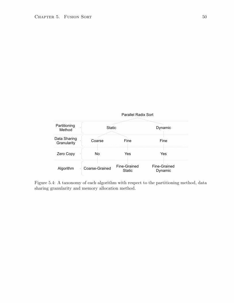
Chapter 5. Fusion Sort 50
Parallel Radix Sort
YesNo
Static Dynamic
Coarse Fine Fine
Yes
Fine-Grained Static
Fine-Grained Dynamic
Coarse-Grained
Data Sharing Granularity
Partitioning Method
Zero Copy
Algorithm
Figure 5.4: A taxonomy of each algorithm with respect to the partitioning method, datasharing granularity and memory allocation method.
Chapter 6
Implementation
In this chapter we present the various implementations of radix sort that were created for
execution on the AMD Fusion APU. We begin by describing reference implementations
that run on only the GPU or CPU devices. We then describe a coarse-grained data
sharing implementation that runs on both the CPU and GPU simultaneously. This
is followed by the introduction three implementations that use fine-grained data sharing
between the GPU and CPU. We conclude by providing a model for a theoretical optimum
sorting implementation using information obtained from the GPU-Only and CPU-Only
implementations.
6.1 GPU-Only Implementation
The GPU-Only implementation closely follows the parallel radix sort algorithm presented
in Section 4.2. This implementation provides a reference against which the performance
of the Fusion Sort algorithms can be measured. As described in Section 4.2, each pass of
the algorithm consists of four basic steps: local sort, histogram, rank, and scatter. Each
of these basic steps is implemented in an OpenCL kernel, the algorithmic details of which
are provided in Section 4.2.
For each kernel, input data is broken into tiles. Each of these tiles is then assigned
51
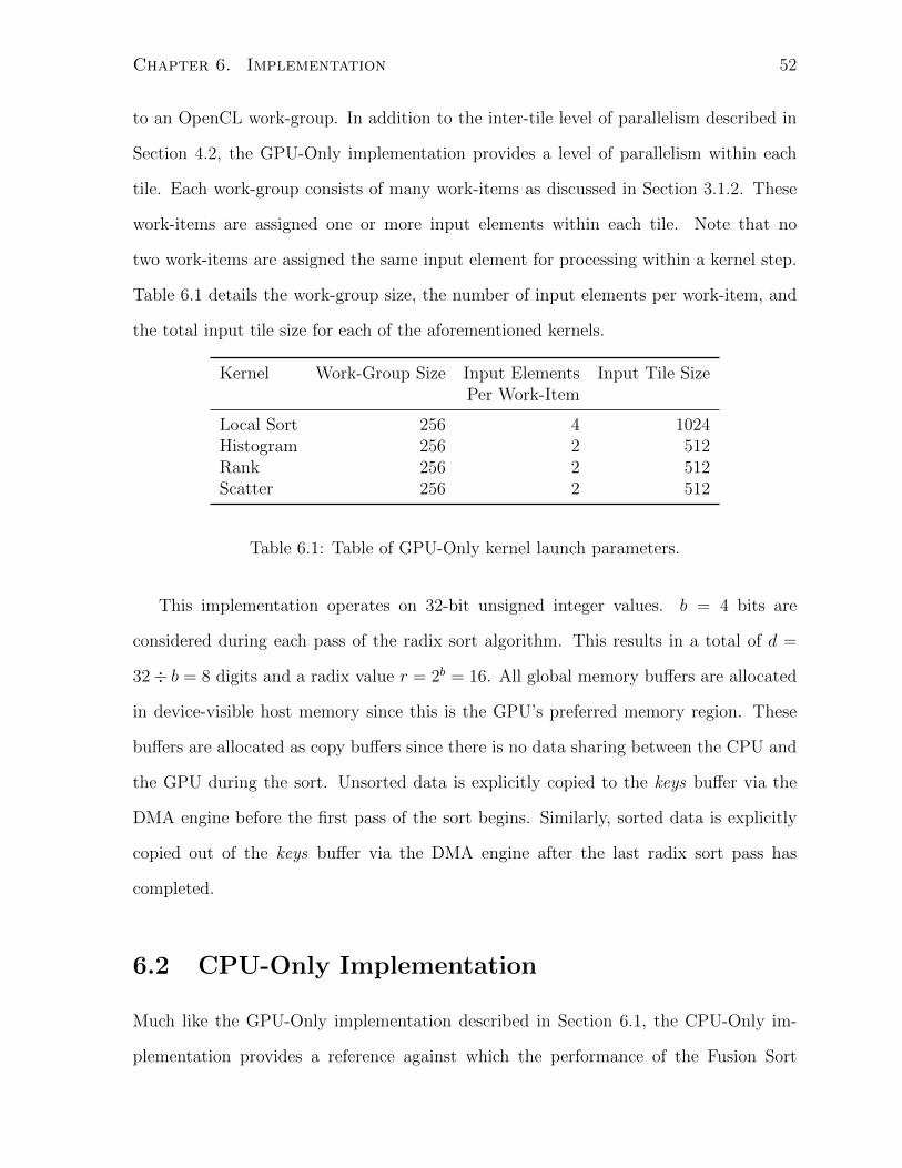
Chapter 6. Implementation 52
to an OpenCL work-group. In addition to the inter-tile level of parallelism described in
Section 4.2, the GPU-Only implementation provides a level of parallelism within each
tile. Each work-group consists of many work-items as discussed in Section 3.1.2. These
work-items are assigned one or more input elements within each tile. Note that no
two work-items are assigned the same input element for processing within a kernel step.
Table 6.1 details the work-group size, the number of input elements per work-item, and
the total input tile size for each of the aforementioned kernels.
Kernel Work-Group Size Input Elements Input Tile SizePer Work-Item
Local Sort 256 4 1024Histogram 256 2 512Rank 256 2 512Scatter 256 2 512
Table 6.1: Table of GPU-Only kernel launch parameters.
This implementation operates on 32-bit unsigned integer values. b = 4 bits are
considered during each pass of the radix sort algorithm. This results in a total of d =
32÷ b = 8 digits and a radix value r = 2b = 16. All global memory buffers are allocated
in device-visible host memory since this is the GPU’s preferred memory region. These
buffers are allocated as copy buffers since there is no data sharing between the CPU and
the GPU during the sort. Unsorted data is explicitly copied to the keys buffer via the
DMA engine before the first pass of the sort begins. Similarly, sorted data is explicitly
copied out of the keys buffer via the DMA engine after the last radix sort pass has
completed.
6.2 CPU-Only Implementation
Much like the GPU-Only implementation described in Section 6.1, the CPU-Only im-
plementation provides a reference against which the performance of the Fusion Sort
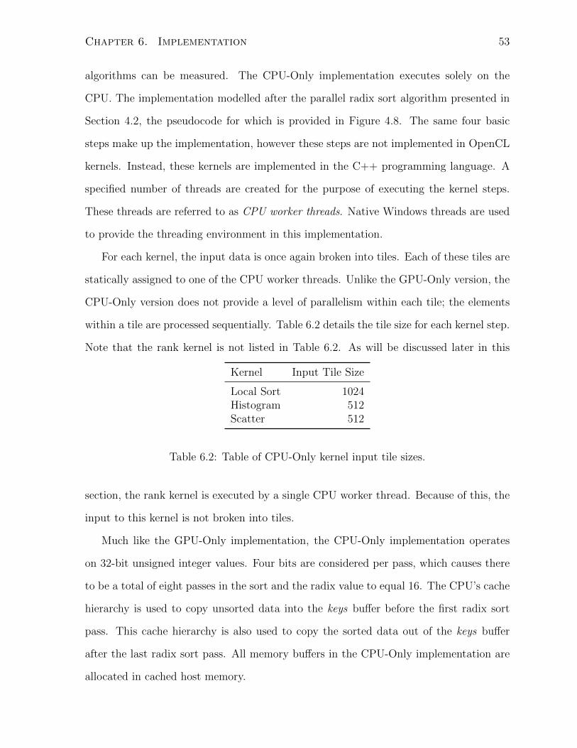
Chapter 6. Implementation 53
algorithms can be measured. The CPU-Only implementation executes solely on the
CPU. The implementation modelled after the parallel radix sort algorithm presented in
Section 4.2, the pseudocode for which is provided in Figure 4.8. The same four basic
steps make up the implementation, however these steps are not implemented in OpenCL
kernels. Instead, these kernels are implemented in the C++ programming language. A
specified number of threads are created for the purpose of executing the kernel steps.
These threads are referred to as CPU worker threads. Native Windows threads are used
to provide the threading environment in this implementation.
For each kernel, the input data is once again broken into tiles. Each of these tiles are
statically assigned to one of the CPU worker threads. Unlike the GPU-Only version, the
CPU-Only version does not provide a level of parallelism within each tile; the elements
within a tile are processed sequentially. Table 6.2 details the tile size for each kernel step.
Note that the rank kernel is not listed in Table 6.2. As will be discussed later in this
Kernel Input Tile Size
Local Sort 1024Histogram 512Scatter 512
Table 6.2: Table of CPU-Only kernel input tile sizes.
section, the rank kernel is executed by a single CPU worker thread. Because of this, the
input to this kernel is not broken into tiles.
Much like the GPU-Only implementation, the CPU-Only implementation operates
on 32-bit unsigned integer values. Four bits are considered per pass, which causes there
to be a total of eight passes in the sort and the radix value to equal 16. The CPU’s cache
hierarchy is used to copy unsorted data into the keys buffer before the first radix sort
pass. This cache hierarchy is also used to copy the sorted data out of the keys buffer
after the last radix sort pass. All memory buffers in the CPU-Only implementation are
allocated in cached host memory.
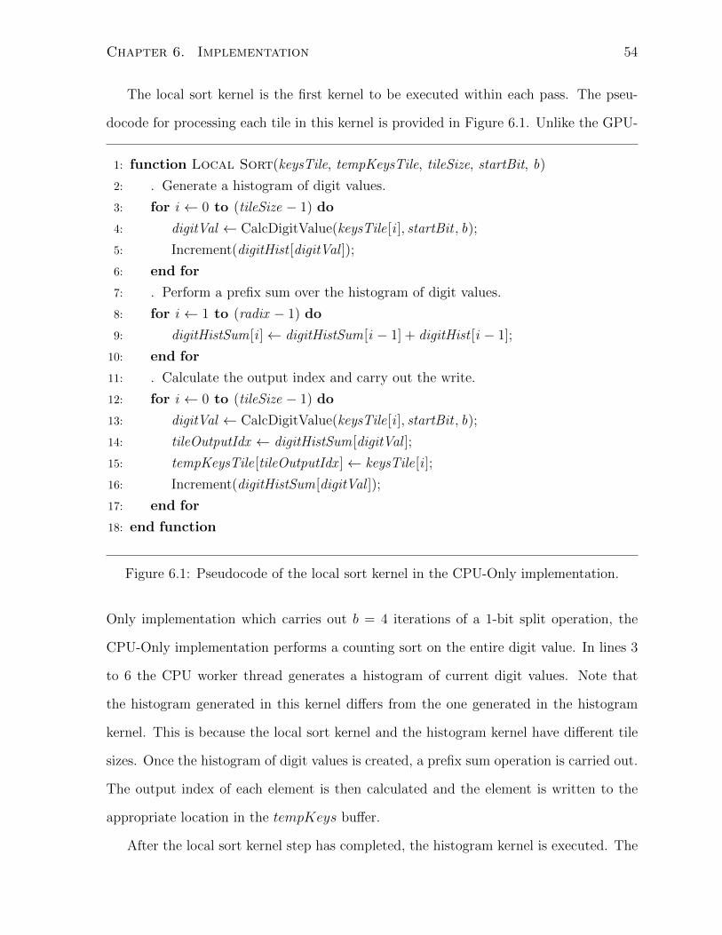
Chapter 6. Implementation 54
The local sort kernel is the first kernel to be executed within each pass. The pseu-
docode for processing each tile in this kernel is provided in Figure 6.1. Unlike the GPU-
1: function Local Sort(keysTile, tempKeysTile, tileSize, startBit, b)
2: . Generate a histogram of digit values.
3: for i ← 0 to (tileSize − 1) do
4: digitVal ← CalcDigitValue(keysTile[i ], startBit , b);
5: Increment(digitHist [digitVal ]);
6: end for
7: . Perform a prefix sum over the histogram of digit values.
8: for i ← 1 to (radix − 1) do
9: digitHistSum[i ]← digitHistSum[i − 1] + digitHist [i − 1];
10: end for
11: . Calculate the output index and carry out the write.
12: for i ← 0 to (tileSize − 1) do
13: digitVal ← CalcDigitValue(keysTile[i ], startBit , b);
14: tileOutputIdx ← digitHistSum[digitVal ];
15: tempKeysTile[tileOutputIdx ]← keysTile[i ];
16: Increment(digitHistSum[digitVal ]);
17: end for
18: end function
Figure 6.1: Pseudocode of the local sort kernel in the CPU-Only implementation.
Only implementation which carries out b = 4 iterations of a 1-bit split operation, the
CPU-Only implementation performs a counting sort on the entire digit value. In lines 3
to 6 the CPU worker thread generates a histogram of current digit values. Note that
the histogram generated in this kernel differs from the one generated in the histogram
kernel. This is because the local sort kernel and the histogram kernel have different tile
sizes. Once the histogram of digit values is created, a prefix sum operation is carried out.
The output index of each element is then calculated and the element is written to the
appropriate location in the tempKeys buffer.
After the local sort kernel step has completed, the histogram kernel is executed. The
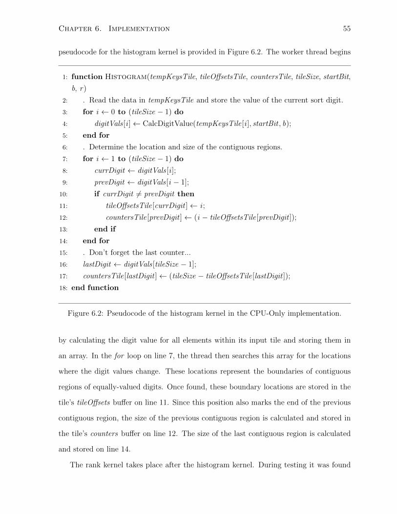
Chapter 6. Implementation 55
pseudocode for the histogram kernel is provided in Figure 6.2. The worker thread begins
1: function Histogram(tempKeysTile, tileOffsetsTile, countersTile, tileSize, startBit,
b, r)
2: . Read the data in tempKeysTile and store the value of the current sort digit.
3: for i ← 0 to (tileSize − 1) do
4: digitVals [i ]← CalcDigitValue(tempKeysTile[i ], startBit , b);
5: end for
6: . Determine the location and size of the contiguous regions.
7: for i ← 1 to (tileSize − 1) do
8: currDigit ← digitVals [i ];
9: prevDigit ← digitVals [i − 1];
10: if currDigit 6= prevDigit then
11: tileOffsetsTile[currDigit ]← i ;
12: countersTile[prevDigit ]← (i − tileOffsetsTile[prevDigit ]);
13: end if
14: end for
15: . Don’t forget the last counter...
16: lastDigit ← digitVals [tileSize − 1];
17: countersTile[lastDigit ]← (tileSize − tileOffsetsTile[lastDigit ]);
18: end function
Figure 6.2: Pseudocode of the histogram kernel in the CPU-Only implementation.
by calculating the digit value for all elements within its input tile and storing them in
an array. In the for loop on line 7, the thread then searches this array for the locations
where the digit values change. These locations represent the boundaries of contiguous
regions of equally-valued digits. Once found, these boundary locations are stored in the
tile’s tileOffsets buffer on line 11. Since this position also marks the end of the previous
contiguous region, the size of the previous contiguous region is calculated and stored in
the tile’s counters buffer on line 12. The size of the last contiguous region is calculated
and stored on line 14.
The rank kernel takes place after the histogram kernel. During testing it was found

Chapter 6. Implementation 56
that this kernel exhibits a lower execution time when carried out by a single thread as
opposed to multiple threads. The rank kernel is therefore executed by a single thread
and the input data is not broken into tiles. The pseudocode for this kernel is provided
in Figure 6.3. The kernel carries out a sequential exclusive prefix sum over all elements
1: function Rank(counters, countersLength, countersSum)
2: for i ← 1 to (countersLength − 1) do
3: countersSum[i ]← (counters [i − 1] + countersSum[i − 1]);
4: end for
5: end function
Figure 6.3: Pseudocode of the rank kernel in the CPU-Only implementation.
in the counters buffer. Once the kernel is complete, the countersSum buffer is populated
with the prefix sum data.
The final step in the CPU-Only implementation is the scatter step. The pseudocode
for this kernel is provided in Figure 6.4. CPU worker threads processes each element in
1: function Scatter(tempKeysTile, tileOffsetsTile, countersSumTile, keys, startBit,
b, elementsPerTile, radix )
2: for i ← 0 to (elementsPerTile − 1) do . For each element in the input tile.
3: . Calculate the current digit value of the current element.
4: digitVal ← CalcDigitValue(tempKeysTile[i ], startBit, b);
5: . Calculate location to scatter the element to.
6: globalOutputIdx ← countersSumTile[digitVal ] + i − tileOffsetsTile[digitVal ];
7: . Perform the scatter write.
8: keys [globalOutputIdx ]← tempKeysTile[i ];
9: end for
10: end function
Figure 6.4: Pseudocode of the scatter kernel in the CPU-Only implementation.
their respective input tiles sequentially. Each thread begins by calculating the current
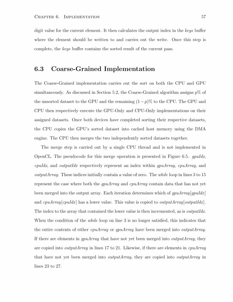
Chapter 6. Implementation 57
digit value for the current element. It then calculates the output index in the keys buffer
where the element should be written to and carries out the write. Once this step is
complete, the keys buffer contains the sorted result of the current pass.
6.3 Coarse-Grained Implementation
The Coarse-Grained implementation carries out the sort on both the CPU and GPU
simultaneously. As discussed in Section 5.2, the Coarse-Grained algorithm assigns p% of
the unsorted dataset to the GPU and the remaining (1−p)% to the CPU. The GPU and
CPU then respectively execute the GPU-Only and CPU-Only implementations on their
assigned datasets. Once both devices have completed sorting their respective datasets,
the CPU copies the GPU’s sorted dataset into cached host memory using the DMA
engine. The CPU then merges the two independently sorted datasets together.
The merge step is carried out by a single CPU thread and is not implemented in
OpenCL. The pseudocode for this merge operation is presented in Figure 6.5. gpuIdx,
cpuIdx, and outputIdx respectively represent an index within gpuArray, cpuArray, and
outputArray. These indices initially contain a value of zero. The while loop in lines 3 to 15
represent the case where both the gpuArray and cpuArray contain data that has not yet
been merged into the output array. Each iteration determines which of gpuArray [gpuIdx ]
and cpuArray [cpuIdx ] has a lower value. This value is copied to outputArray [outputIdx ].
The index to the array that contained the lower value is then incremented, as is outputIdx.
When the condition of the while loop on line 3 is no longer satisfied, this indicates that
the entire contents of either cpuArray or gpuArray have been merged into outputArray.
If there are elements in gpuArray that have not yet been merged into outputArray, they
are copied into outputArray in lines 17 to 21. Likewise, if there are elements in cpuArray
that have not yet been merged into outputArray, they are copied into outputArray in
lines 23 to 27.
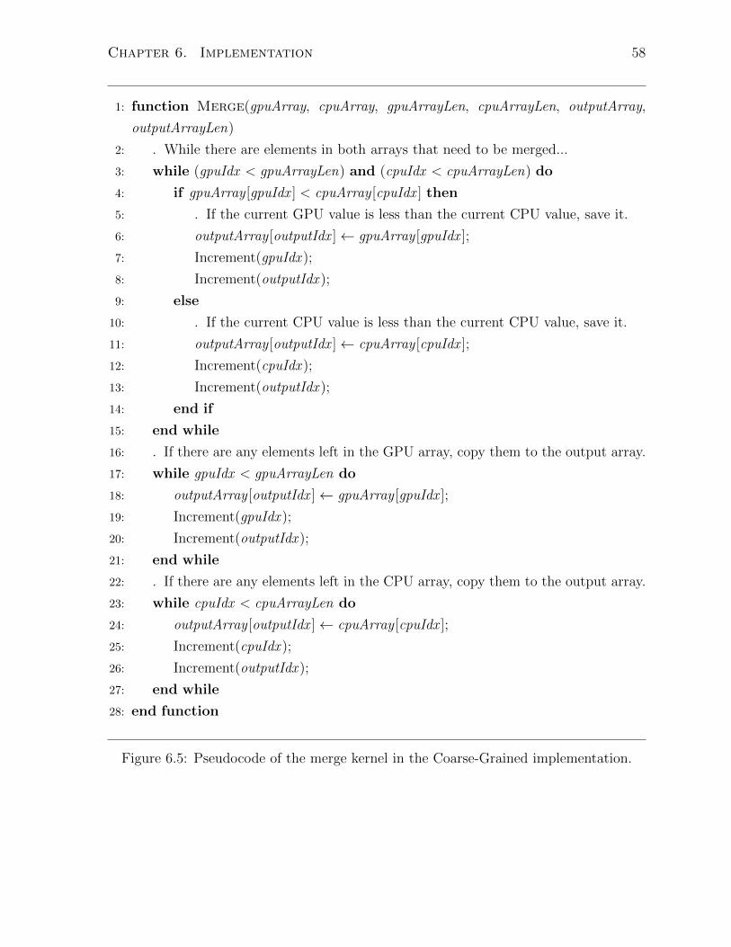
Chapter 6. Implementation 58
1: function Merge(gpuArray, cpuArray, gpuArrayLen, cpuArrayLen, outputArray,
outputArrayLen)
2: . While there are elements in both arrays that need to be merged...
3: while (gpuIdx < gpuArrayLen) and (cpuIdx < cpuArrayLen) do
4: if gpuArray [gpuIdx ] < cpuArray [cpuIdx ] then
5: . If the current GPU value is less than the current CPU value, save it.
6: outputArray [outputIdx ]← gpuArray [gpuIdx ];
7: Increment(gpuIdx );
8: Increment(outputIdx );
9: else
10: . If the current CPU value is less than the current CPU value, save it.
11: outputArray [outputIdx ]← cpuArray [cpuIdx ];
12: Increment(cpuIdx );
13: Increment(outputIdx );
14: end if
15: end while
16: . If there are any elements left in the GPU array, copy them to the output array.
17: while gpuIdx < gpuArrayLen do
18: outputArray [outputIdx ]← gpuArray [gpuIdx ];
19: Increment(gpuIdx );
20: Increment(outputIdx );
21: end while
22: . If there are any elements left in the CPU array, copy them to the output array.
23: while cpuIdx < cpuArrayLen do
24: outputArray [outputIdx ]← cpuArray [cpuIdx ];
25: Increment(cpuIdx );
26: Increment(outputIdx );
27: end while
28: end function
Figure 6.5: Pseudocode of the merge kernel in the Coarse-Grained implementation.

Chapter 6. Implementation 59
6.4 Fine-Grained Static Implementation
Much like the Coarse-Grained implementation, the Fine-Grained Static implementation
executes its sort on both the CPU and GPU simultaneously. As described in Section 5.3,
each pass of the algorithm consists of the local sort kernel, histogram kernel, rank kernel,
and scatter kernel. The unsorted input data is broken into tiles and p% of the tiles are
assigned to the GPU for processing. The remaining (1− p)% are assigned to the CPU.
The GPU’s kernel steps are implemented in OpenCL while the CPU’s kernel steps
are implemented in C++ using native Windows threads. The launch parameters per-
taining to the GPU kernels do not differ from the GPU-Only implementation and can be
found in Table 6.1. Likewise, the tile sizes used in the CPU’s kernel steps are provided
in Table 6.2. The GPU and CPU kernel steps are modelled after the GPU-Only and
CPU-Only implementations, the algorithmic details of which are respectively provided
in Sections 4.2 and 6.2. Where necessary, additional information has been provided in
each kernel to ensure that the GPU accounts for the number of tiles that have been
assigned to the CPU and vice-versa. Much like the aforementioned implementations, the
Fine-Grained Static implementation operates on 32-bit unsigned integer values. b = 4
bits are considered during each pass of the parallel radix sort algorithm. This results in
a total of d = 32÷ b = 8 digits and a radix value of r = 2b = 16.
The implementation of the Fine-Grained Static algorithm deviates slightly from the
algorithmic description provided in Section 5.3. During implementation it was discovered
that splitting the rank step across the CPU and GPU requires a significant amount of
synchronization between the devices. Additionally, extra computational steps would need
to be introduced in order to carry out the rank step across both devices. It was therefore
decided that the rank step would be entirely carried out by only one device. The rank
step in the CPU-Only implementation was empirically found to be faster than the rank
step in the GPU-Only implementation. The CPU was therefore chosen to carry out
the entire rank operation in the Fine-Grained Static implementation. This rank step
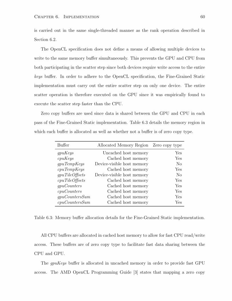
Chapter 6. Implementation 60
is carried out in the same single-threaded manner as the rank operation described in
Section 6.2.
The OpenCL specification does not define a means of allowing multiple devices to
write to the same memory buffer simultaneously. This prevents the GPU and CPU from
both participating in the scatter step since both devices require write access to the entire
keys buffer. In order to adhere to the OpenCL specification, the Fine-Grained Static
implementation must carry out the entire scatter step on only one device. The entire
scatter operation is therefore executed on the GPU since it was empirically found to
execute the scatter step faster than the CPU.
Zero copy buffers are used since data is shared between the GPU and CPU in each
pass of the Fine-Grained Static implementation. Table 6.3 details the memory region in
which each buffer is allocated as well as whether not a buffer is of zero copy type.
Buffer Allocated Memory Region Zero copy type
gpuKeys Uncached host memory YescpuKeys Cached host memory YesgpuTempKeys Device-visible host memory NocpuTempKeys Cached host memory YesgpuTileOffsets Device-visible host memory NocpuTileOffsets Cached host memory YesgpuCounters Cached host memory YescpuCounters Cached host memory YesgpuCountersSum Cached host memory YescpuCountersSum Cached host memory Yes
Table 6.3: Memory buffer allocation details for the Fine-Grained Static implementation.
All CPU buffers are allocated in cached host memory to allow for fast CPU read/write
access. These buffers are of zero copy type to facilitate fast data sharing between the
CPU and GPU.
The gpuKeys buffer is allocated in uncached memory in order to provide fast GPU
access. The AMD OpenCL Programming Guide [3] states that mapping a zero copy
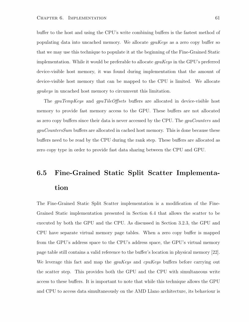
Chapter 6. Implementation 61
buffer to the host and using the CPU’s write combining buffers is the fastest method of
populating data into uncached memory. We allocate gpuKeys as a zero copy buffer so
that we may use this technique to populate it at the beginning of the Fine-Grained Static
implementation. While it would be preferable to allocate gpuKeys in the GPU’s preferred
device-visible host memory, it was found during implementation that the amount of
device-visible host memory that can be mapped to the CPU is limited. We allocate
gpukeys in uncached host memory to circumvent this limitation.
The gpuTempKeys and gpuTileOffsets buffers are allocated in device-visible host
memory to provide fast memory access to the GPU. These buffers are not allocated
as zero copy buffers since their data is never accessed by the CPU. The gpuCounters and
gpuCountersSum buffers are allocated in cached host memory. This is done because these
buffers need to be read by the CPU during the rank step. These buffers are allocated as
zero copy type in order to provide fast data sharing between the CPU and GPU.
6.5 Fine-Grained Static Split Scatter Implementa-
tion
The Fine-Grained Static Split Scatter implementation is a modification of the Fine-
Grained Static implementation presented in Section 6.4 that allows the scatter to be
executed by both the GPU and the CPU. As discussed in Section 3.2.3, the GPU and
CPU have separate virtual memory page tables. When a zero copy buffer is mapped
from the GPU’s address space to the CPU’s address space, the GPU’s virtual memory
page table still contains a valid reference to the buffer’s location in physical memory [22].
We leverage this fact and map the gpuKeys and cpuKeys buffers before carrying out
the scatter step. This provides both the GPU and the CPU with simultaneous write
access to these buffers. It is important to note that while this technique allows the GPU
and CPU to access data simultaneously on the AMD Llano architecture, its behaviour is
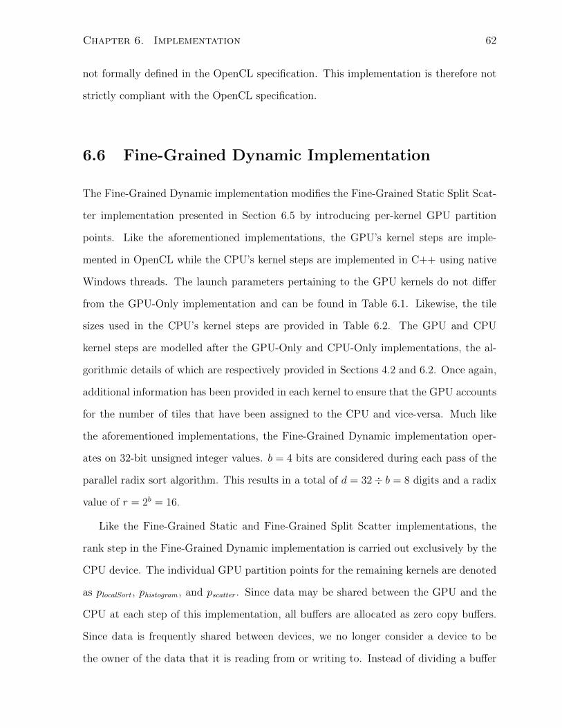
Chapter 6. Implementation 62
not formally defined in the OpenCL specification. This implementation is therefore not
strictly compliant with the OpenCL specification.
6.6 Fine-Grained Dynamic Implementation
The Fine-Grained Dynamic implementation modifies the Fine-Grained Static Split Scat-
ter implementation presented in Section 6.5 by introducing per-kernel GPU partition
points. Like the aforementioned implementations, the GPU’s kernel steps are imple-
mented in OpenCL while the CPU’s kernel steps are implemented in C++ using native
Windows threads. The launch parameters pertaining to the GPU kernels do not differ
from the GPU-Only implementation and can be found in Table 6.1. Likewise, the tile
sizes used in the CPU’s kernel steps are provided in Table 6.2. The GPU and CPU
kernel steps are modelled after the GPU-Only and CPU-Only implementations, the al-
gorithmic details of which are respectively provided in Sections 4.2 and 6.2. Once again,
additional information has been provided in each kernel to ensure that the GPU accounts
for the number of tiles that have been assigned to the CPU and vice-versa. Much like
the aforementioned implementations, the Fine-Grained Dynamic implementation oper-
ates on 32-bit unsigned integer values. b = 4 bits are considered during each pass of the
parallel radix sort algorithm. This results in a total of d = 32÷ b = 8 digits and a radix
value of r = 2b = 16.
Like the Fine-Grained Static and Fine-Grained Split Scatter implementations, the
rank step in the Fine-Grained Dynamic implementation is carried out exclusively by the
CPU device. The individual GPU partition points for the remaining kernels are denoted
as plocalSort , phistogram , and pscatter . Since data may be shared between the GPU and the
CPU at each step of this implementation, all buffers are allocated as zero copy buffers.
Since data is frequently shared between devices, we no longer consider a device to be
the owner of the data that it is reading from or writing to. Instead of dividing a buffer
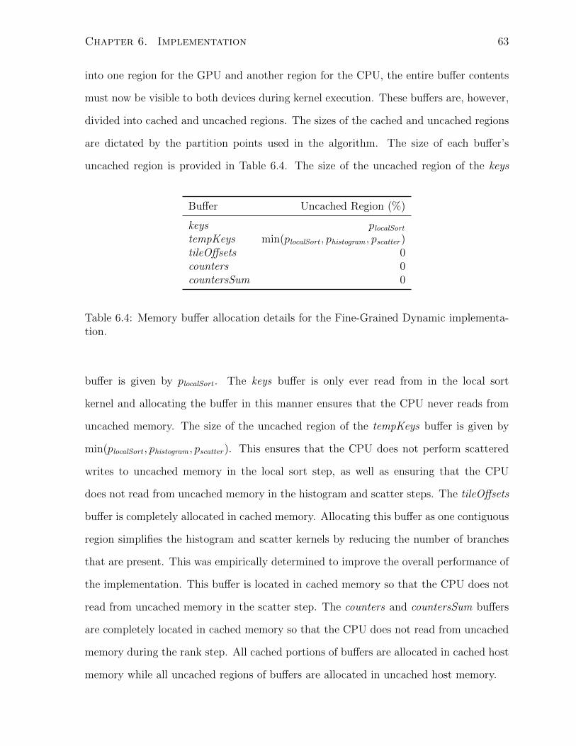
Chapter 6. Implementation 63
into one region for the GPU and another region for the CPU, the entire buffer contents
must now be visible to both devices during kernel execution. These buffers are, however,
divided into cached and uncached regions. The sizes of the cached and uncached regions
are dictated by the partition points used in the algorithm. The size of each buffer’s
uncached region is provided in Table 6.4. The size of the uncached region of the keys
Buffer Uncached Region (%)
keys plocalSorttempKeys min(plocalSort , phistogram , pscatter)tileOffsets 0counters 0countersSum 0
Table 6.4: Memory buffer allocation details for the Fine-Grained Dynamic implementa-tion.
buffer is given by plocalSort . The keys buffer is only ever read from in the local sort
kernel and allocating the buffer in this manner ensures that the CPU never reads from
uncached memory. The size of the uncached region of the tempKeys buffer is given by
min(plocalSort , phistogram , pscatter). This ensures that the CPU does not perform scattered
writes to uncached memory in the local sort step, as well as ensuring that the CPU
does not read from uncached memory in the histogram and scatter steps. The tileOffsets
buffer is completely allocated in cached memory. Allocating this buffer as one contiguous
region simplifies the histogram and scatter kernels by reducing the number of branches
that are present. This was empirically determined to improve the overall performance of
the implementation. This buffer is located in cached memory so that the CPU does not
read from uncached memory in the scatter step. The counters and countersSum buffers
are completely located in cached memory so that the CPU does not read from uncached
memory during the rank step. All cached portions of buffers are allocated in cached host
memory while all uncached regions of buffers are allocated in uncached host memory.

Chapter 6. Implementation 64
6.7 Theoretical Optimum Model
The theoretical optimum is modelled after the dataflow that is present in the Fine-
Grained Dynamic Algorithm described in Section 5.4. Its purpose is to model the execu-
tion time of the Fine-Grained Dynamic implementation without the overhead of memory
accesses to non-preferred memory regions or the management of multiple devices and
data buffers. This model should provide the lowest theoretically attainable execution
time of the Fine-Grained Dynamic implementation.
This model assumes that per-kernel partitioning is taking place at the optimal parti-
tion point for all partitioned kernels. We define the optimal partition point for a given
kernel as the GPU partition point that minimizes that kernel’s execution time. It models
a sort implementation where all memory accesses are done to each device’s preferred
memory region. It also models a sort where there is no additional complexity involved
in having both the GPU and CPU participate in kernel steps simultaneously. Note that
these characteristics are present in the GPU-Only and CPU-Only implementations.
Consider sorting N elements using the Fine-Grained Dynamic implementation. We
determine the theoretically optimum execution time of a given kernel step by first plotting
the GPU-Only implementation’s corresponding kernel execution time as a function of
n where n varies between 0 and N . We then plot the CPU-Only implementation’s
corresponding kernel execution time as a function of N −n where n varies between 0 and
N . The result is illustrated in Figure 6.6. Once these values are plotted, the execution
time of the theoretical model is given by the maximum execution time at each simulated
partition point. The theoretical optimum execution time is found where the execution
time of the GPU kernel is equal to that of the CPU kernel. We do this for the local sort,
histogram, and scatter kernels in order to determine the theoretical optimum execution
time for each of them. We perform an analogous operation to determine the theoretical
optimum execution time for the initial population of data the keys buffer and the final
retrieval of sorted data from the keys buffer. Since the rank step is only carried out on
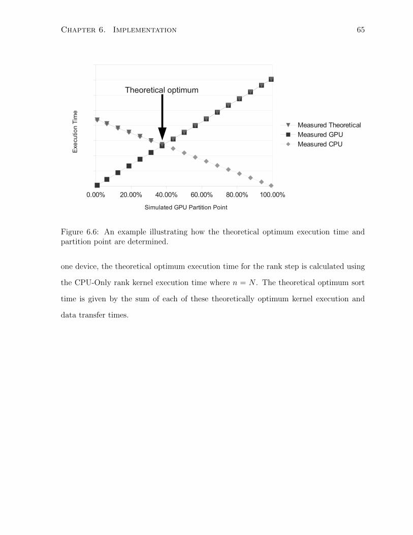
Chapter 6. Implementation 65
0.00% 20.00% 40.00% 60.00% 80.00% 100.00%
Measured Theoretical
Measured GPU
Measured CPU
Simulated GPU Partition Point
Exe
cutio
n T
ime
Theoretical optimum
Figure 6.6: An example illustrating how the theoretical optimum execution time andpartition point are determined.
one device, the theoretical optimum execution time for the rank step is calculated using
the CPU-Only rank kernel execution time where n = N . The theoretical optimum sort
time is given by the sum of each of these theoretically optimum kernel execution and
data transfer times.
Chapter 7
Evaluation
In this chapter we present the experimental evaluation of several radix sort implementa-
tions. We begin by describing the hardware and software platforms used in the evaluation.
We then define the performance metrics that will be used throughout the remainder of
the chapter. Finally, we provide the evaluation methodology and results for each of the
implementations described in Chapter 6.
7.1 Hardware Platforms
Each version of radix sort was evaluated on two hardware platforms. The specifications
of the platforms are similar, however the APU model varies between them. One platform
contains an A6-3650 model APU while the other contains an A8-3850 model APU. There
are several differences between these APU models that affect their relative CPU and GPU
performance. The CPU in the A6-3650 contains four cores, each with a clock speed of
2.6 GHz [5]. The CPU in the A8-3850 also contains four cores, however these cores clock
at 2.9 GHz. The GPU in the A8-3850 contains 400 cores, each of which have a clock
speed of 600 MHz. The GPU in the A6-3650 contains 320 cores that clock at 443 MHz.
The result is that the GPU in the A8-3850 has 25% more cores than the A6-3650, each
of which has a clock speed that is 35.4% faster than the A6-3650. In contrast, the
66

Chapter 7. Evaluation 67
CPU in the A8-3850 has an equal number of cores to the A6-3650, each of which has
a clock speed that is 11.5% faster than the A6-3650. Note the A8-3850 shows a higher
percent increase in GPU core count and clock speed than CPU core count and clock
speed when compared to the A6-3650. The complete specifications of the two platforms
are summarized in Table 7.1.
Hardware Specification Platform 1 Platform 2
APU model A6-3650 A8-3850CPU cores 4 4CPU frequency 2.6 GHz 2.9 GHzGPU model HD 6530D HD 6550DGPU cores 320 400GPU core frequency 443 MHz 600 MHzAPU DRAM type DDR3 DDR3APU DRAM frequency 1866 MHz 1866 MHzAPU DRAM size 8 GB 8 GBHost memory size 6 GB 6 GBDevice memory size 2 GB 2 GB
Table 7.1: Summary of evaluation platforms.
7.2 Software Platform
Each of the GPU’s radix sort kernels is implemented using OpenCL C. The OpenCL
C++ bindings are used in the host code. The CPU’s radix sort kernels and control flow
code are written in C++. The OpenCL runtime and compilers are provided by version
2.6 of the AMD Accelerated Parallel Processing Software Development Kit [9] and version
11.12 of the AMD Catalyst driver suite [15]. All tests were run under Microsoft Windows
7 64-bit. All code that executes on the CPU was compiled using the Microsoft Visual
Studio 2010 C++ compiler with /O2 optimizations enabled. Native Windows threads
were used to provide the threading environment on the CPU.
Chapter 7. Evaluation 68
7.3 Performance Metrics
The sort time of the algorithm is measured when conducting each experiment. We define
sort time as the time it takes to copy the unsorted keys into the input keys buffer, carry
out the sort operation, and read the sorted data back from the output keys buffer. Sort
time is always measured using the CPU’s high-resolution performance counter.
Where appropriate, kernel execution time and data transfer time are also measured.
When an OpenCL kernel or OpenCL memory command is submitted to the GPU, a
corresponding OpenCL event object is generated, as discussed in Section 3.1.2 These
events are queried to determine the execution time of OpenCL kernels that execute on
the GPU. This execution time is measured using the GPU’s internal timer. Data transfers
that use the DMA engine are also measured using this method since they are initiated
in the form of OpenCL memory commands.
OpenCL events are generated when buffers are mapped to and unmapped from the
CPU’s address space, however no OpenCL event is generated when the CPU transfers
data to or from a mapped buffer. We therefore use the CPU’s high-resolution performance
counter to determine the execution time of data transfers that take place to mapped zero
copy memory buffers. This same performance counter is used to determine the execution
time of kernel steps that execute on the CPU.
Sort time and kernel execution time are used to calculate throughput. We define
throughput as follows:
throughput =number of input elements
time
When calculating throughput for the entire sort algorithm, the number of input elements
refers to the number of elements that are to be sorted. When determining the throughput
of the local sort kernel, the number of input elements refers to the number of elements in
the kernel’s keys input buffer that are to be locally sorted. In the context of the histogram
kernel’s throughput, the number of input elements equals the number of locally sorted
Chapter 7. Evaluation 69
elements in the kernel’s tempKeys input buffer for which histogram and tile offset data
will be generated. When referring to throughput for the rank kernel, the number of
input elements refers to the number of elements in the kernel’s counters input buffer over
which a prefix sum operation is performed. When calculating throughput for the scatter
kernel, the number of input elements refers to the number of locally sorted elements in
the kernel’s tempKeys input buffer that are to be scattered to the output keys buffer.
Sort time and execution time are also used to calculate the speedup of the sorting
implementation or kernel step. We define speedup with respect to a baseline as follows:
speedup =baseline time
measured time
In addition to sort time and execution time, we also measure idle time when it is
appropriate. Idle time represents the amount of time that one device remains idle while
the other device executes a step in the sorting algorithm. For a given kernel step k,
let the kernel execution time on the GPU and CPU be represented as tkGPUand tkCPU
,
respectively. The idle time that is present during the execution of kernel step k is given
by:
idle time = |tkGPU− tkCPU
|
where |x| represents the absolute value of x.
7.4 Evaluated Implementations
In the following sections, we specifically evaluate the following versions of radix sort:
GPU-Only, CPU-Only, Coarse-Grained, Fine-Grained Static, Fine-Grained Static Split
Scatter, Fine-Grained Dynamic, and Measured Theoretical Optimum. Each of these ver-
sions are described in detail in Chapter 6 of this document.
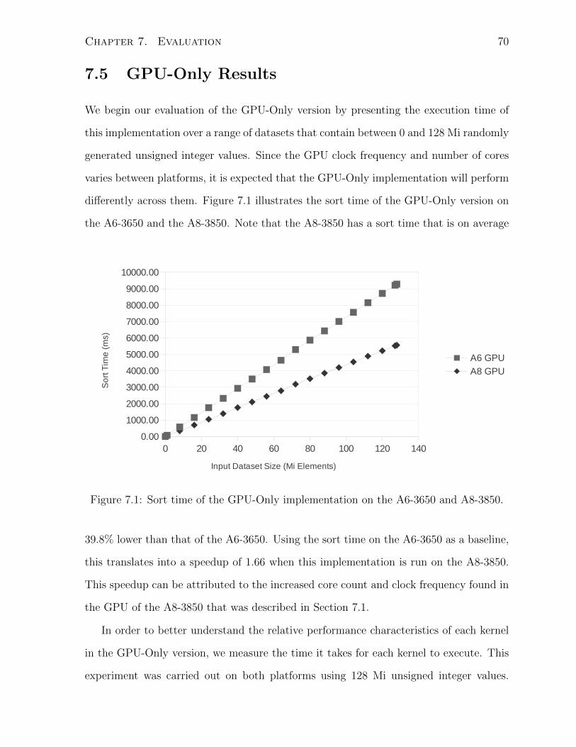
Chapter 7. Evaluation 70
7.5 GPU-Only Results
We begin our evaluation of the GPU-Only version by presenting the execution time of
this implementation over a range of datasets that contain between 0 and 128 Mi randomly
generated unsigned integer values. Since the GPU clock frequency and number of cores
varies between platforms, it is expected that the GPU-Only implementation will perform
differently across them. Figure 7.1 illustrates the sort time of the GPU-Only version on
the A6-3650 and the A8-3850. Note that the A8-3850 has a sort time that is on average
0 20 40 60 80 100 120 1400.00
1000.00
2000.00
3000.00
4000.00
5000.00
6000.00
7000.00
8000.00
9000.00
10000.00
A6 GPU
A8 GPU
Input Dataset Size (Mi Elements)
So
rt T
ime
(m
s)
Figure 7.1: Sort time of the GPU-Only implementation on the A6-3650 and A8-3850.
39.8% lower than that of the A6-3650. Using the sort time on the A6-3650 as a baseline,
this translates into a speedup of 1.66 when this implementation is run on the A8-3850.
This speedup can be attributed to the increased core count and clock frequency found in
the GPU of the A8-3850 that was described in Section 7.1.
In order to better understand the relative performance characteristics of each kernel
in the GPU-Only version, we measure the time it takes for each kernel to execute. This
experiment was carried out on both platforms using 128 Mi unsigned integer values.
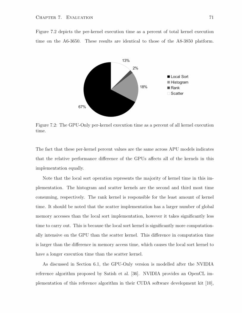
Chapter 7. Evaluation 71
Figure 7.2 depicts the per-kernel execution time as a percent of total kernel execution
time on the A6-3650. These results are identical to those of the A8-3850 platform.
67%
18%
2%
13%
Local Sort
Histogram
Rank
Scatter
Figure 7.2: The GPU-Only per-kernel execution time as a percent of all kernel executiontime.
The fact that these per-kernel percent values are the same across APU models indicates
that the relative performance difference of the GPUs affects all of the kernels in this
implementation equally.
Note that the local sort operation represents the majority of kernel time in this im-
plementation. The histogram and scatter kernels are the second and third most time
consuming, respectively. The rank kernel is responsible for the least amount of kernel
time. It should be noted that the scatter implementation has a larger number of global
memory accesses than the local sort implementation, however it takes significantly less
time to carry out. This is because the local sort kernel is significantly more computation-
ally intensive on the GPU than the scatter kernel. This difference in computation time
is larger than the difference in memory access time, which causes the local sort kernel to
have a longer execution time than the scatter kernel.
As discussed in Section 6.1, the GPU-Only version is modelled after the NVIDIA
reference algorithm proposed by Satish et al. [36]. NVIDIA provides an OpenCL im-
plementation of this reference algorithm in their CUDA software development kit [10],
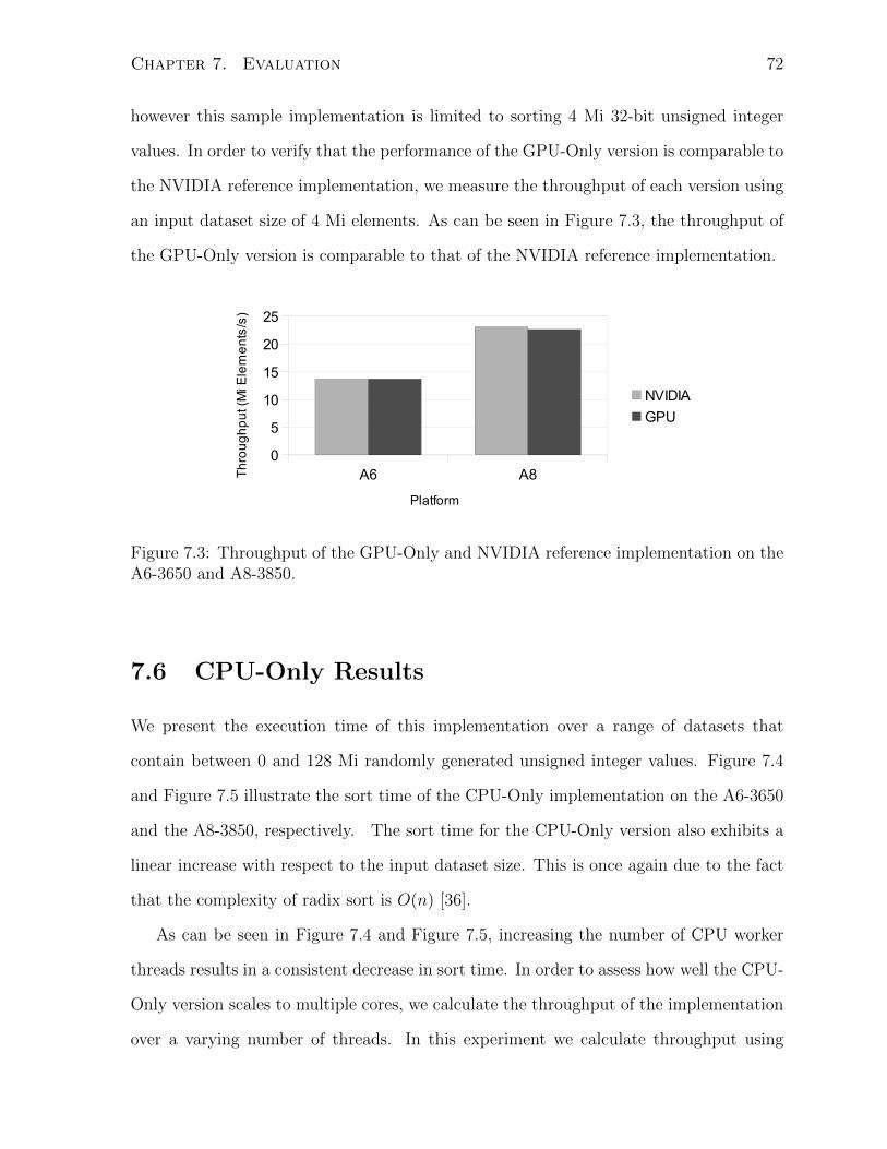
Chapter 7. Evaluation 72
however this sample implementation is limited to sorting 4 Mi 32-bit unsigned integer
values. In order to verify that the performance of the GPU-Only version is comparable to
the NVIDIA reference implementation, we measure the throughput of each version using
an input dataset size of 4 Mi elements. As can be seen in Figure 7.3, the throughput of
the GPU-Only version is comparable to that of the NVIDIA reference implementation.
A6 A80
5
10
15
20
25
NVIDIA
GPU-Only
Platform
Th
rou
gh
pu
t (M
i Ele
me
nts
/s)
A6 A80
5
10
15
20
25
NVIDIA
GPU
Platform
Th
rou
gh
pu
t (M
i Ele
me
nts
/s)
Figure 7.3: Throughput of the GPU-Only and NVIDIA reference implementation on theA6-3650 and A8-3850.
7.6 CPU-Only Results
We present the execution time of this implementation over a range of datasets that
contain between 0 and 128 Mi randomly generated unsigned integer values. Figure 7.4
and Figure 7.5 illustrate the sort time of the CPU-Only implementation on the A6-3650
and the A8-3850, respectively. The sort time for the CPU-Only version also exhibits a
linear increase with respect to the input dataset size. This is once again due to the fact
that the complexity of radix sort is O(n) [36].
As can be seen in Figure 7.4 and Figure 7.5, increasing the number of CPU worker
threads results in a consistent decrease in sort time. In order to assess how well the CPU-
Only version scales to multiple cores, we calculate the throughput of the implementation
over a varying number of threads. In this experiment we calculate throughput using
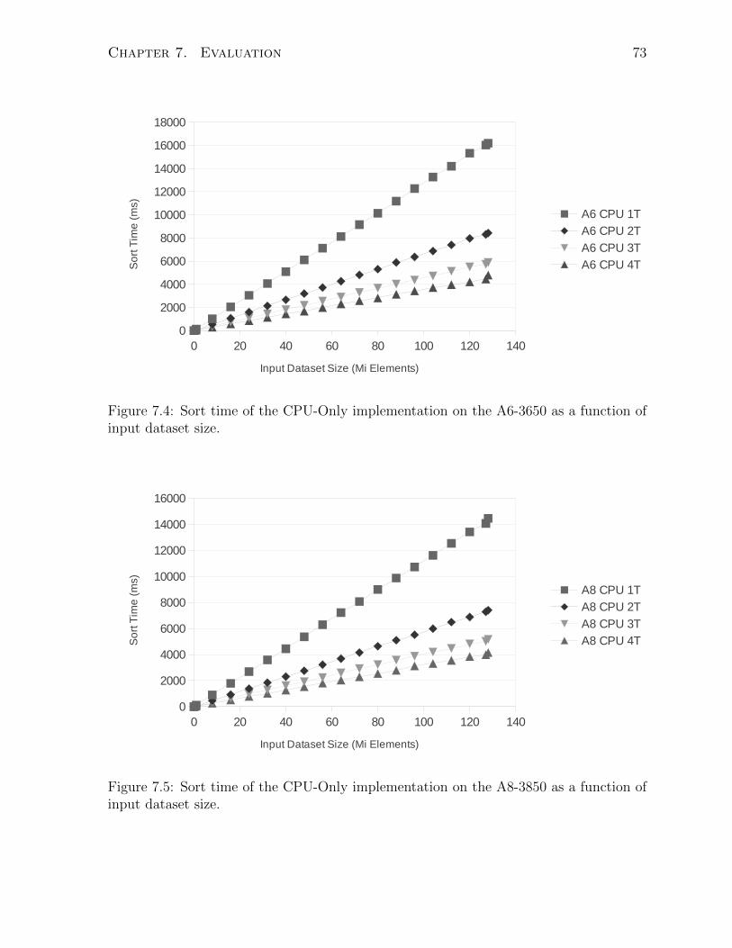
Chapter 7. Evaluation 73
0 20 40 60 80 100 120 1400
2000
4000
6000
8000
10000
12000
14000
16000
18000
A6 CPU 1T
A6 CPU 2T
A6 CPU 3T
A6 CPU 4T
Input Dataset Size (Mi Elements)
So
rt T
ime
(m
s)
Figure 7.4: Sort time of the CPU-Only implementation on the A6-3650 as a function ofinput dataset size.
0 20 40 60 80 100 120 1400
2000
4000
6000
8000
10000
12000
14000
16000
A8 CPU 1T
A8 CPU 2T
A8 CPU 3T
A8 CPU 4T
Input Dataset Size (Mi Elements)
So
rt T
ime
(m
s)
Figure 7.5: Sort time of the CPU-Only implementation on the A8-3850 as a function ofinput dataset size.
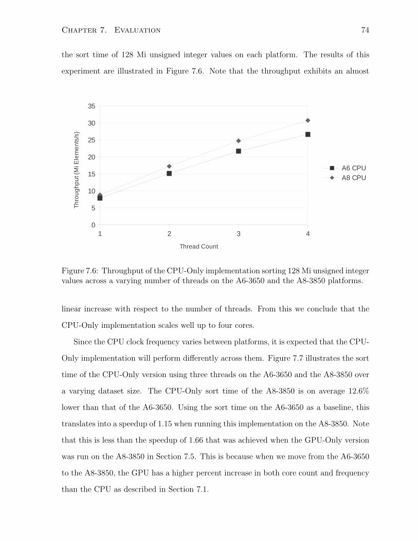
Chapter 7. Evaluation 74
the sort time of 128 Mi unsigned integer values on each platform. The results of this
experiment are illustrated in Figure 7.6. Note that the throughput exhibits an almost
1 2 3 40
5
10
15
20
25
30
35
A6 CPU
A8 CPU
Thread Count
Th
rou
gh
pu
t (M
i Ele
me
nts
/s)
Figure 7.6: Throughput of the CPU-Only implementation sorting 128 Mi unsigned integervalues across a varying number of threads on the A6-3650 and the A8-3850 platforms.
linear increase with respect to the number of threads. From this we conclude that the
CPU-Only implementation scales well up to four cores.
Since the CPU clock frequency varies between platforms, it is expected that the CPU-
Only implementation will perform differently across them. Figure 7.7 illustrates the sort
time of the CPU-Only version using three threads on the A6-3650 and the A8-3850 over
a varying dataset size. The CPU-Only sort time of the A8-3850 is on average 12.6%
lower than that of the A6-3650. Using the sort time on the A6-3650 as a baseline, this
translates into a speedup of 1.15 when running this implementation on the A8-3850. Note
that this is less than the speedup of 1.66 that was achieved when the GPU-Only version
was run on the A8-3850 in Section 7.5. This is because when we move from the A6-3650
to the A8-3850, the GPU has a higher percent increase in both core count and frequency
than the CPU as described in Section 7.1.
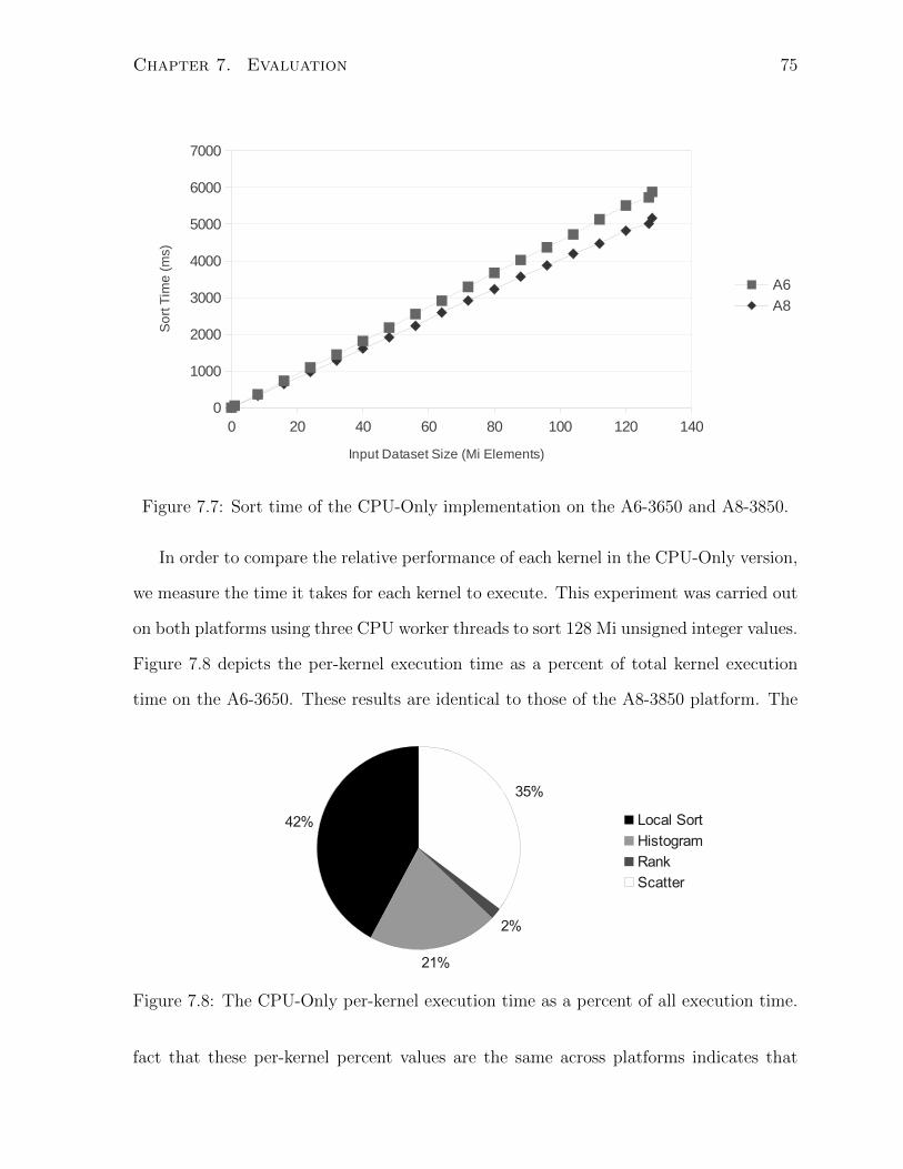
Chapter 7. Evaluation 75
0 20 40 60 80 100 120 1400
1000
2000
3000
4000
5000
6000
7000
A6
A8
Input Dataset Size (Mi Elements)
So
rt T
ime
(m
s)
Figure 7.7: Sort time of the CPU-Only implementation on the A6-3650 and A8-3850.
In order to compare the relative performance of each kernel in the CPU-Only version,
we measure the time it takes for each kernel to execute. This experiment was carried out
on both platforms using three CPU worker threads to sort 128 Mi unsigned integer values.
Figure 7.8 depicts the per-kernel execution time as a percent of total kernel execution
time on the A6-3650. These results are identical to those of the A8-3850 platform. The
42%
21%
2%
35%
Local Sort
Histogram
Rank
Scatter
Figure 7.8: The CPU-Only per-kernel execution time as a percent of all execution time.
fact that these per-kernel percent values are the same across platforms indicates that
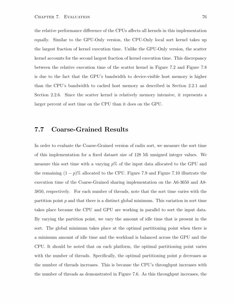
Chapter 7. Evaluation 76
the relative performance difference of the CPUs affects all kernels in this implementation
equally. Similar to the GPU-Only version, the CPU-Only local sort kernel takes up
the largest fraction of kernel execution time. Unlike the GPU-Only version, the scatter
kernel accounts for the second largest fraction of kernel execution time. This discrepancy
between the relative execution time of the scatter kernel in Figure 7.2 and Figure 7.8
is due to the fact that the GPU’s bandwidth to device-visible host memory is higher
than the CPU’s bandwidth to cached host memory as described in Section 2.2.1 and
Section 2.2.6. Since the scatter kernel is relatively memory intensive, it represents a
larger percent of sort time on the CPU than it does on the GPU.
7.7 Coarse-Grained Results
In order to evaluate the Coarse-Grained version of radix sort, we measure the sort time
of this implementation for a fixed dataset size of 128 Mi unsigned integer values. We
measure this sort time with a varying p% of the input data allocated to the GPU and
the remaining (1 − p)% allocated to the CPU. Figure 7.9 and Figure 7.10 illustrate the
execution time of the Coarse-Grained sharing implementation on the A6-3650 and A8-
3850, respectively. For each number of threads, note that the sort time varies with the
partition point p and that there is a distinct global minimum. This variation in sort time
takes place because the CPU and GPU are working in parallel to sort the input data.
By varying the partition point, we vary the amount of idle time that is present in the
sort. The global minimum takes place at the optimal partitioning point when there is
a minimum amount of idle time and the workload is balanced across the GPU and the
CPU. It should be noted that on each platform, the optimal partitioning point varies
with the number of threads. Specifically, the optimal partitioning point p decreases as
the number of threads increases. This is because the CPU’s throughput increases with
the number of threads as demonstrated in Figure 7.6. As this throughput increases, the
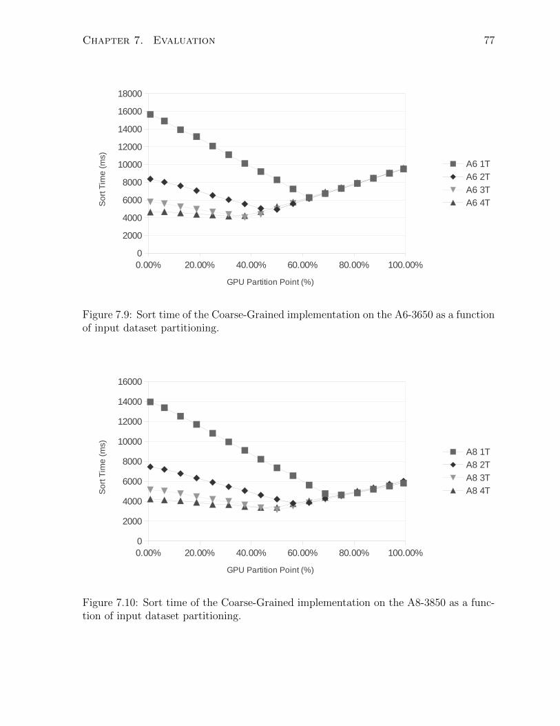
Chapter 7. Evaluation 77
0.00% 20.00% 40.00% 60.00% 80.00% 100.00%0
2000
4000
6000
8000
10000
12000
14000
16000
18000
A6 1T
A6 2T
A6 3T
A6 4T
GPU Partition Point (%)
So
rt T
ime
(m
s)
Figure 7.9: Sort time of the Coarse-Grained implementation on the A6-3650 as a functionof input dataset partitioning.
0.00% 20.00% 40.00% 60.00% 80.00% 100.00%0
2000
4000
6000
8000
10000
12000
14000
16000
A8 1T
A8 2T
A8 3T
A8 4T
GPU Partition Point (%)
So
rt T
ime
(m
s)
Figure 7.10: Sort time of the Coarse-Grained implementation on the A8-3850 as a func-tion of input dataset partitioning.

Chapter 7. Evaluation 78
GPU must be assigned a smaller percent of the input dataset to prevent the introduction
of CPU idle time. There is, however, one exception to this. When the Coarse-Grained
implementation runs with four CPU worker threads, the partition point does not move
significantly. When a program makes use of the AMD OpenCL runtime, a background
thread is created to manage the OpenCL device. This thread polls the device’s status
and is responsible for enqueueing tasks to the device. The issue of thread contention
for CPU cores arises when the Coarse-Grained sorting implementation is run with four
CPU worker threads. GPU performance can degrade if the OpenCL background thread
becomes starved. Conversely, CPU performance can degrade if the OpenCL background
thread is not starved. When running the Coarse-Grained implementation with four CPU
worker threads, these factors result in a large variation in sort time and optimal partition
point from one iteration to the next. From this we conclude that the Coarse-Grained
implementation does not scale well to four CPU worker threads on both the A6-3650 and
the A8-3850.
For each number of threads, the optimal partitioning point also varies across plat-
forms. For a given number of threads, the optimal partitioning point is lower on the
A6-3650 than on the A8-3850. This can be seen in Figure 7.11, which depicts the sort
time of 128 Mi unsigned integer values using three CPU worker threads across the two
APU platforms. This fluctuation in optimal partition point takes place because the rel-
ative performance of the CPU and GPU are not equal across platforms as discussed in
Section 7.1 and Section 7.6. When run with three CPU worker threads, the optimal par-
tition point is at 38% on the A6-3650 and 50% on the A8-3850. This indicates that the
CPU-Only and GPU-Only radix sort performance is more balanced across the A8-3850’s
CPU and GPU than the A6-3650.
Since the two APU models exhibit different performance characteristics and have
different optimal partition points, we expect the overall sort time to vary between them as
well. This is evident in in Figure 7.11, which shows the sort time of 128 Mi elements using
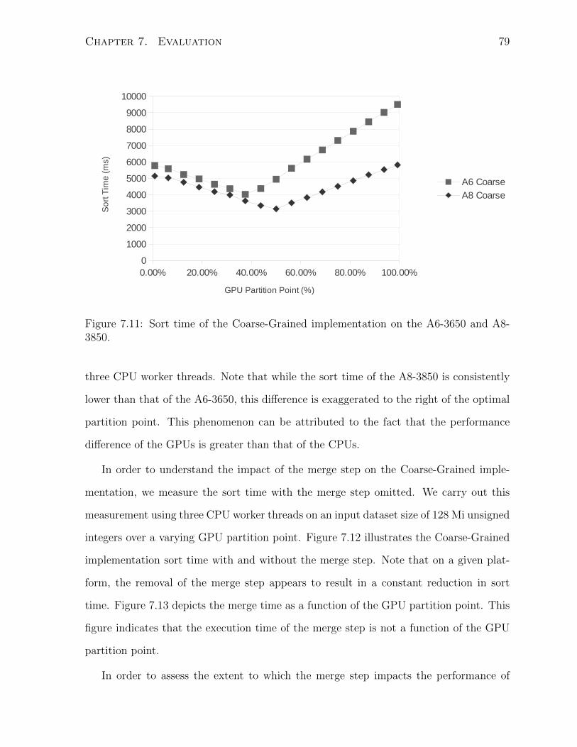
Chapter 7. Evaluation 79
0.00% 20.00% 40.00% 60.00% 80.00% 100.00%0
1000
2000
3000
4000
5000
6000
7000
8000
9000
10000
A6 Coarse
A8 Coarse
GPU Partition Point (%)
So
rt T
ime
(m
s)
Figure 7.11: Sort time of the Coarse-Grained implementation on the A6-3650 and A8-3850.
three CPU worker threads. Note that while the sort time of the A8-3850 is consistently
lower than that of the A6-3650, this difference is exaggerated to the right of the optimal
partition point. This phenomenon can be attributed to the fact that the performance
difference of the GPUs is greater than that of the CPUs.
In order to understand the impact of the merge step on the Coarse-Grained imple-
mentation, we measure the sort time with the merge step omitted. We carry out this
measurement using three CPU worker threads on an input dataset size of 128 Mi unsigned
integers over a varying GPU partition point. Figure 7.12 illustrates the Coarse-Grained
implementation sort time with and without the merge step. Note that on a given plat-
form, the removal of the merge step appears to result in a constant reduction in sort
time. Figure 7.13 depicts the merge time as a function of the GPU partition point. This
figure indicates that the execution time of the merge step is not a function of the GPU
partition point.
In order to assess the extent to which the merge step impacts the performance of
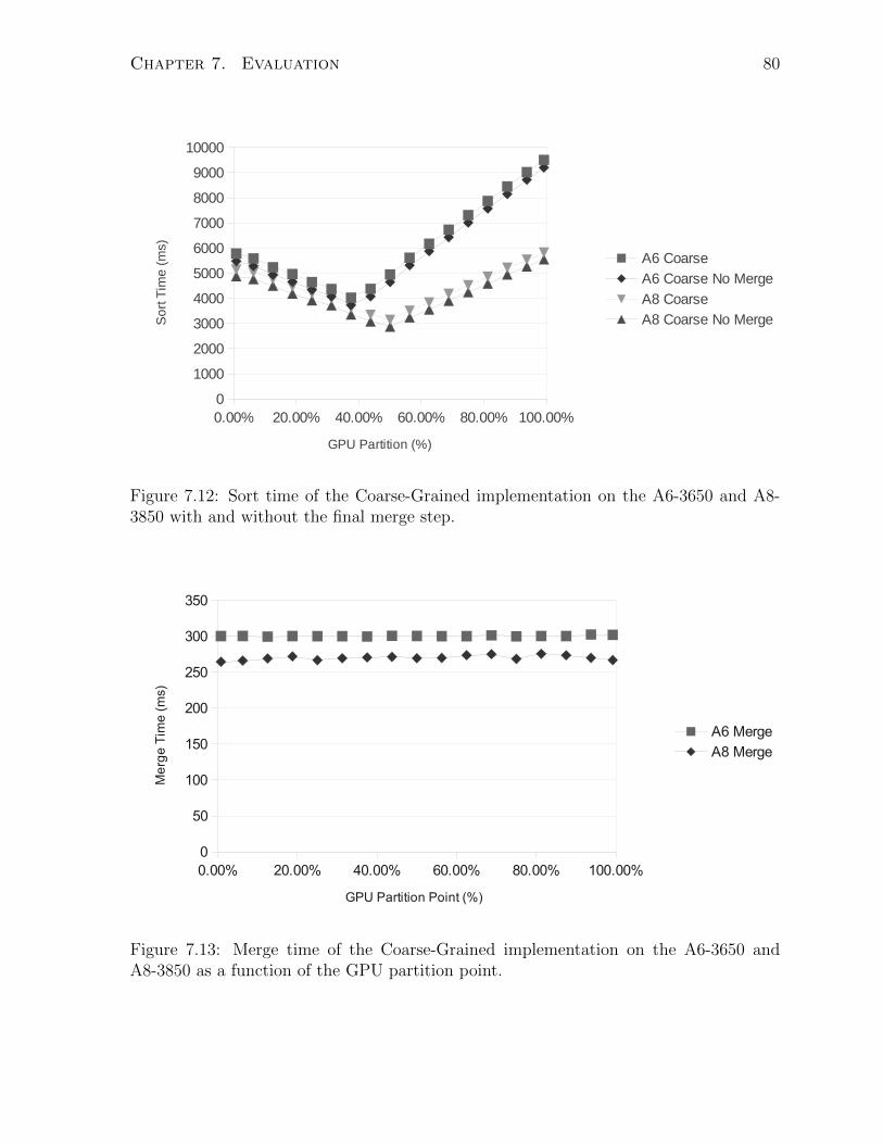
Chapter 7. Evaluation 80
0.00% 20.00% 40.00% 60.00% 80.00% 100.00%0
1000
2000
3000
4000
5000
6000
7000
8000
9000
10000
A6 Coarse
A6 Coarse No Merge
A8 Coarse
A8 Coarse No Merge
GPU Partition (%)
So
rt T
ime
(m
s)
Figure 7.12: Sort time of the Coarse-Grained implementation on the A6-3650 and A8-3850 with and without the final merge step.
0.00% 20.00% 40.00% 60.00% 80.00% 100.00%0
50
100
150
200
250
300
350
A6 Merge
A8 Merge
GPU Partition Point (%)
Me
rge
Tim
e (
ms)
Figure 7.13: Merge time of the Coarse-Grained implementation on the A6-3650 andA8-3850 as a function of the GPU partition point.
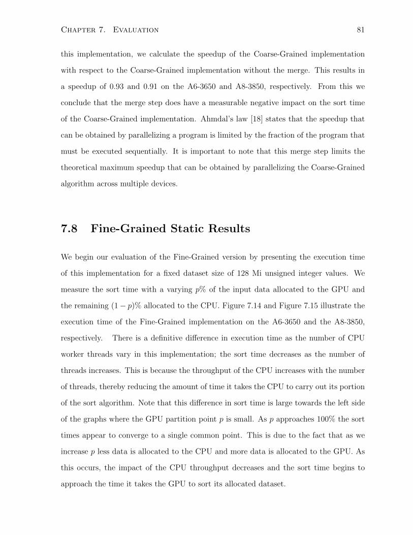
Chapter 7. Evaluation 81
this implementation, we calculate the speedup of the Coarse-Grained implementation
with respect to the Coarse-Grained implementation without the merge. This results in
a speedup of 0.93 and 0.91 on the A6-3650 and A8-3850, respectively. From this we
conclude that the merge step does have a measurable negative impact on the sort time
of the Coarse-Grained implementation. Ahmdal’s law [18] states that the speedup that
can be obtained by parallelizing a program is limited by the fraction of the program that
must be executed sequentially. It is important to note that this merge step limits the
theoretical maximum speedup that can be obtained by parallelizing the Coarse-Grained
algorithm across multiple devices.
7.8 Fine-Grained Static Results
We begin our evaluation of the Fine-Grained version by presenting the execution time
of this implementation for a fixed dataset size of 128 Mi unsigned integer values. We
measure the sort time with a varying p% of the input data allocated to the GPU and
the remaining (1− p)% allocated to the CPU. Figure 7.14 and Figure 7.15 illustrate the
execution time of the Fine-Grained implementation on the A6-3650 and the A8-3850,
respectively. There is a definitive difference in execution time as the number of CPU
worker threads vary in this implementation; the sort time decreases as the number of
threads increases. This is because the throughput of the CPU increases with the number
of threads, thereby reducing the amount of time it takes the CPU to carry out its portion
of the sort algorithm. Note that this difference in sort time is large towards the left side
of the graphs where the GPU partition point p is small. As p approaches 100% the sort
times appear to converge to a single common point. This is due to the fact that as we
increase p less data is allocated to the CPU and more data is allocated to the GPU. As
this occurs, the impact of the CPU throughput decreases and the sort time begins to
approach the time it takes the GPU to sort its allocated dataset.
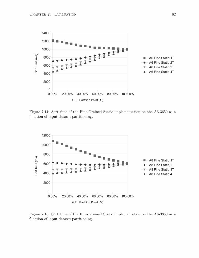
Chapter 7. Evaluation 82
0.00% 20.00% 40.00% 60.00% 80.00% 100.00%0
2000
4000
6000
8000
10000
12000
14000
A6 Fine Static 1T
A6 Fine Static 2T
A6 Fine Static 3T
A6 Fine Static 4T
GPU Partition Point (%)
So
rt T
ime
(m
s)
Figure 7.14: Sort time of the Fine-Grained Static implementation on the A6-3650 as afunction of input dataset partitioning.
0.00% 20.00% 40.00% 60.00% 80.00% 100.00%0
2000
4000
6000
8000
10000
12000
A8 Fine Static 1T
A8 Fine Static 2T
A8 Fine Static 3T
A8 Fine Static 4T
GPU Partition Point (%)
So
rt T
ime
(m
s)
Figure 7.15: Sort time of the Fine-Grained Static implementation on the A8-3850 as afunction of input dataset partitioning.
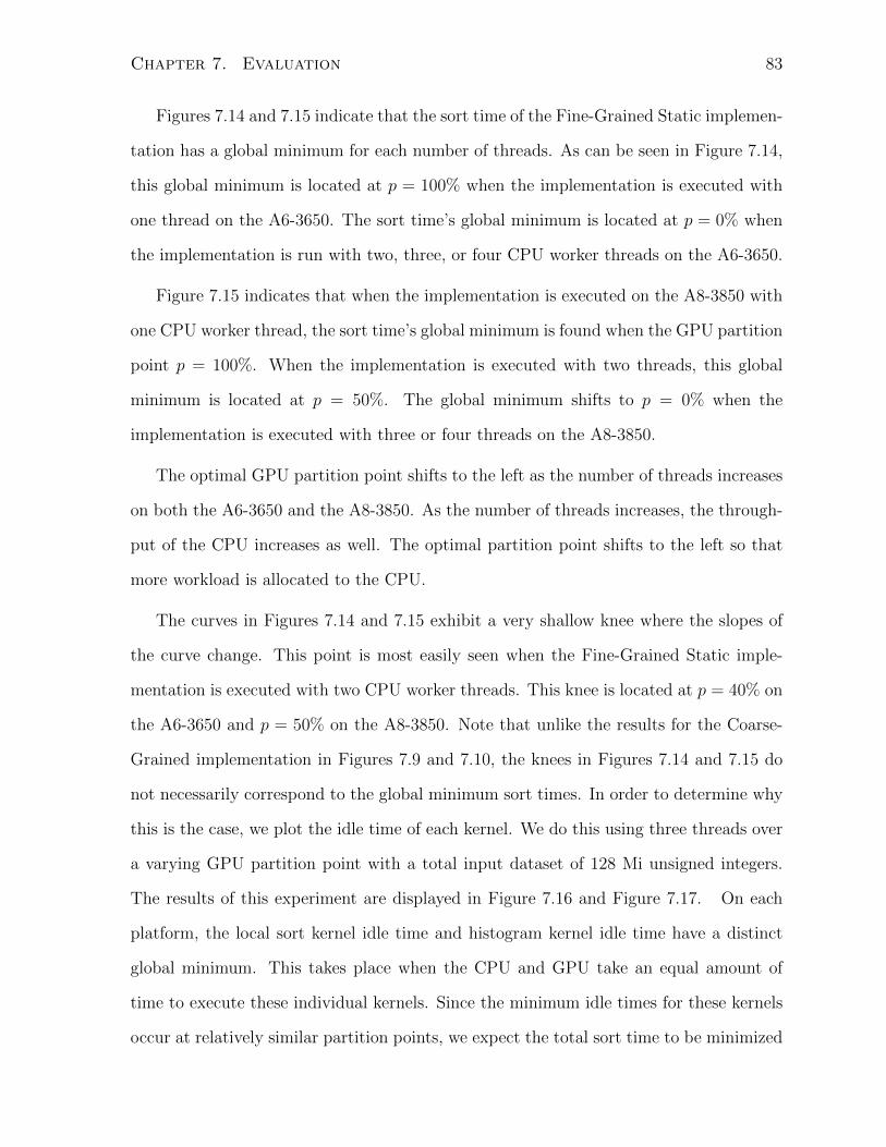
Chapter 7. Evaluation 83
Figures 7.14 and 7.15 indicate that the sort time of the Fine-Grained Static implemen-
tation has a global minimum for each number of threads. As can be seen in Figure 7.14,
this global minimum is located at p = 100% when the implementation is executed with
one thread on the A6-3650. The sort time’s global minimum is located at p = 0% when
the implementation is run with two, three, or four CPU worker threads on the A6-3650.
Figure 7.15 indicates that when the implementation is executed on the A8-3850 with
one CPU worker thread, the sort time’s global minimum is found when the GPU partition
point p = 100%. When the implementation is executed with two threads, this global
minimum is located at p = 50%. The global minimum shifts to p = 0% when the
implementation is executed with three or four threads on the A8-3850.
The optimal GPU partition point shifts to the left as the number of threads increases
on both the A6-3650 and the A8-3850. As the number of threads increases, the through-
put of the CPU increases as well. The optimal partition point shifts to the left so that
more workload is allocated to the CPU.
The curves in Figures 7.14 and 7.15 exhibit a very shallow knee where the slopes of
the curve change. This point is most easily seen when the Fine-Grained Static imple-
mentation is executed with two CPU worker threads. This knee is located at p = 40% on
the A6-3650 and p = 50% on the A8-3850. Note that unlike the results for the Coarse-
Grained implementation in Figures 7.9 and 7.10, the knees in Figures 7.14 and 7.15 do
not necessarily correspond to the global minimum sort times. In order to determine why
this is the case, we plot the idle time of each kernel. We do this using three threads over
a varying GPU partition point with a total input dataset of 128 Mi unsigned integers.
The results of this experiment are displayed in Figure 7.16 and Figure 7.17. On each
platform, the local sort kernel idle time and histogram kernel idle time have a distinct
global minimum. This takes place when the CPU and GPU take an equal amount of
time to execute these individual kernels. Since the minimum idle times for these kernels
occur at relatively similar partition points, we expect the total sort time to be minimized
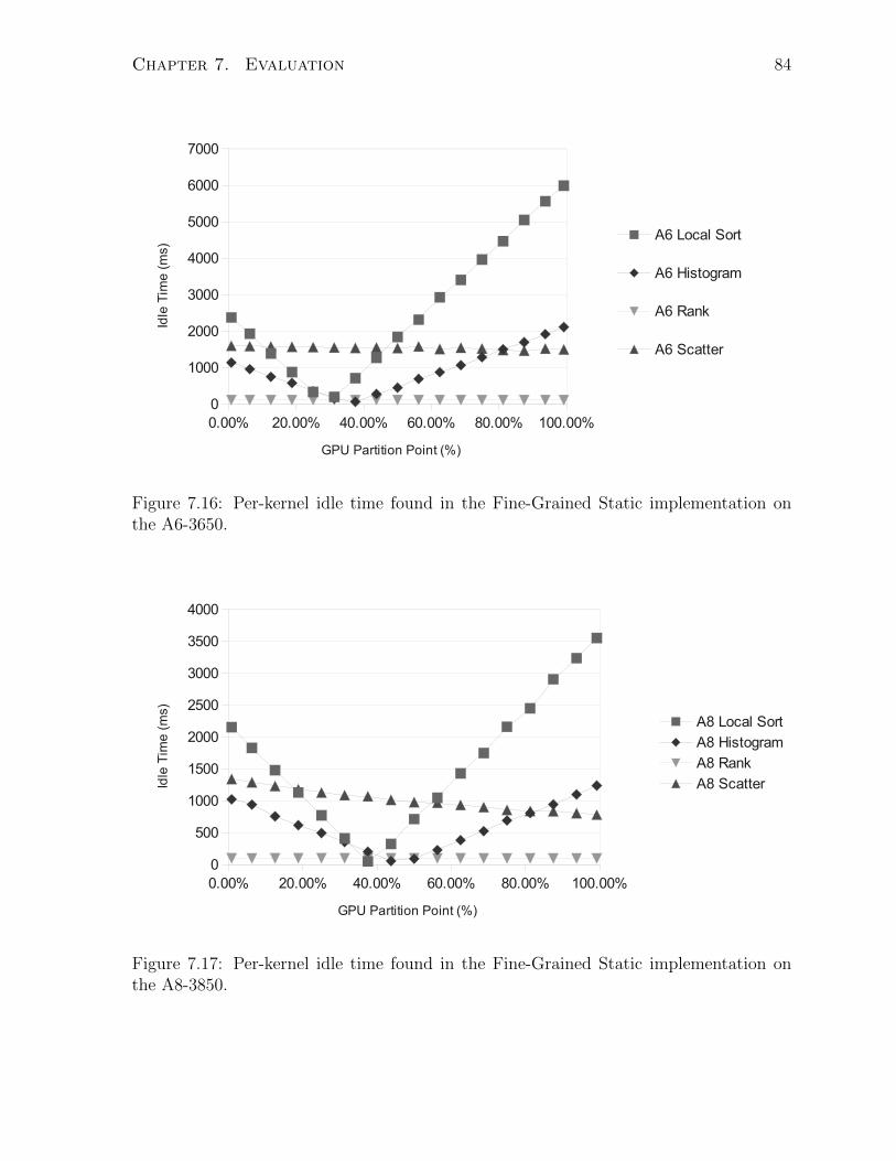
Chapter 7. Evaluation 84
0.00% 20.00% 40.00% 60.00% 80.00% 100.00%0
1000
2000
3000
4000
5000
6000
7000
A6 Local Sort
A6 Histogram
A6 Rank
A6 Scatter
GPU Partition Point (%)
Idle
Tim
e (
ms)
Figure 7.16: Per-kernel idle time found in the Fine-Grained Static implementation onthe A6-3650.
0.00% 20.00% 40.00% 60.00% 80.00% 100.00%0
500
1000
1500
2000
2500
3000
3500
4000
A8 Local Sort
A8 Histogram
A8 Rank
A8 Scatter
GPU Partition Point (%)
Idle
Tim
e (
ms)
Figure 7.17: Per-kernel idle time found in the Fine-Grained Static implementation onthe A8-3850.
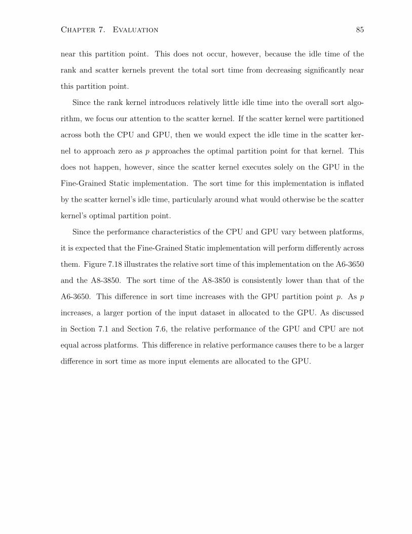
Chapter 7. Evaluation 85
near this partition point. This does not occur, however, because the idle time of the
rank and scatter kernels prevent the total sort time from decreasing significantly near
this partition point.
Since the rank kernel introduces relatively little idle time into the overall sort algo-
rithm, we focus our attention to the scatter kernel. If the scatter kernel were partitioned
across both the CPU and GPU, then we would expect the idle time in the scatter ker-
nel to approach zero as p approaches the optimal partition point for that kernel. This
does not happen, however, since the scatter kernel executes solely on the GPU in the
Fine-Grained Static implementation. The sort time for this implementation is inflated
by the scatter kernel’s idle time, particularly around what would otherwise be the scatter
kernel’s optimal partition point.
Since the performance characteristics of the CPU and GPU vary between platforms,
it is expected that the Fine-Grained Static implementation will perform differently across
them. Figure 7.18 illustrates the relative sort time of this implementation on the A6-3650
and the A8-3850. The sort time of the A8-3850 is consistently lower than that of the
A6-3650. This difference in sort time increases with the GPU partition point p. As p
increases, a larger portion of the input dataset in allocated to the GPU. As discussed
in Section 7.1 and Section 7.6, the relative performance of the GPU and CPU are not
equal across platforms. This difference in relative performance causes there to be a larger
difference in sort time as more input elements are allocated to the GPU.

Chapter 7. Evaluation 86
0.00% 20.00% 40.00% 60.00% 80.00% 100.00%0
2000
4000
6000
8000
10000
12000
A6 Fine Static 3T
A8 Fine Static 3T
GPU Partition Point (%)
So
rt T
ime
(m
s)
Figure 7.18: Sort time of the Fine-Grained Static implementation on the A6-3650 andthe A8-3850 as a function of input dataset partitioning.
7.9 Fine-Grained Static Split Scatter Results
Here we measure the Fine-Grained Static Split Scatter implementation sort time of 128 Mi
unsigned integer values. We measure this sort time with a varying p% of the input dataset
allocated to the GPU and the remaining (1−p)% allocated to the CPU. The results of this
experiment are presented in Figure 7.19 and Figure 7.20. Much like the Fine-Grained
Static implementation, the sort time varies with the GPU partition point p. Unlike the
Fine-Grained Static implementation, however, the sort times do not generally follow a
linear trend. For each number of threads there is an optimal partition point p where the
sort time is minimized.
In Figure 7.19 and Figure 7.20 the sort time varies as a function of the optimal GPU
partition point p. This is caused by the idle time that is introduced at each partition
point. Additionally, the sort time varies as a function of the number of CPU worker
threads. As the number of CPU worker threads increases, the sort time at the optimal
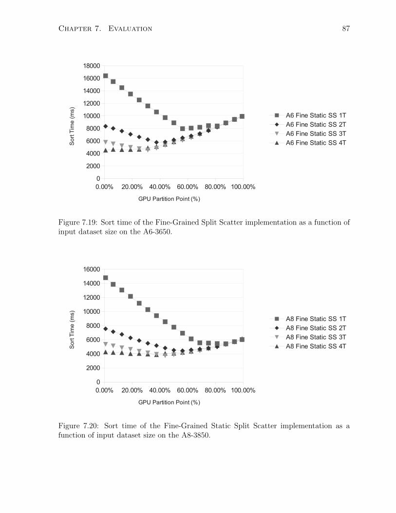
Chapter 7. Evaluation 87
0.00% 20.00% 40.00% 60.00% 80.00% 100.00%0
2000
4000
6000
8000
10000
12000
14000
16000
18000
A6 Fine Static SS 1T
A6 Fine Static SS 2T
A6 Fine Static SS 3T
A6 Fine Static SS 4T
GPU Partition Point (%)
So
rt T
ime
(m
s)
Figure 7.19: Sort time of the Fine-Grained Split Scatter implementation as a function ofinput dataset size on the A6-3650.
0.00% 20.00% 40.00% 60.00% 80.00% 100.00%0
2000
4000
6000
8000
10000
12000
14000
16000
A8 Fine Static SS 1T
A8 Fine Static SS 2T
A8 Fine Static SS 3T
A8 Fine Static SS 4T
GPU Partition Point (%)
So
rt T
ime
(m
s)
Figure 7.20: Sort time of the Fine-Grained Static Split Scatter implementation as afunction of input dataset size on the A8-3850.
Chapter 7. Evaluation 88
partition point decreases. This is true when running the sort implementation with three
CPU worker threads or fewer. When the sort implementation is run with four CPU
worker threads, sort time at the optimal partitioning point is greater than when it is run
with three threads. As described in Section 7.7, we encounter thread contention for CPU
cores when the implementation is run with four threads. Because a background device
management thread is launched by the AMD OpenCL runtime. When this occurs, there
are more busy threads than available CPU cores. Because the CPU cores have been over
allocated, the sort time at the optimal partition point increases. From this we conclude
that this implementation does not scale well to four CPU worker threads on the platforms
that were tested.
For a given number of threads, the optimal partition point and sort time vary across
APU models. In Figure 7.21 we plot the sort time of 128 Mi elements over a varying GPU
partition point using three threads on both the A6-3650 and the A8-3850. In this figure,
0.00% 20.00% 40.00% 60.00% 80.00% 100.00%0
2000
4000
6000
8000
10000
12000
A6 Fine Static Sscat 3T
A8 Fine Static Sscat 3T
GPU Partition Point (%)
So
rt T
ime
(m
s)
Figure 7.21: Sort time of the Fine-Grained Split Scatter implementation on the A6-3650and A8-3850.
the A8-3850 consistently achieves a lower sort time than the A6-3650. This is because

Chapter 7. Evaluation 89
the CPU and GPU of the A8-3850 are capable of executing the individual sort kernels
faster than the CPU and GPU of the A6-3650. The optimal partitioning point also
varies from one platform to the other. This is once again due to the fact that the relative
performance of the CPU and GPU is not constant across APU models as presented in
Section 7.1 and Section 7.6. This causes the optimal partitioning point to be higher on
the A8-3850 than on the A6-3650.
In order to assess the specific impact of allowing both the CPU and GPU to participate
in the scatter step, we measure the per-kernel idle times when using three threads to
sort 128 Mi elements. The results of this experiment are illustrated in Figure 7.22 and
Figure 7.23. As these figures illustrate, there is an optimal partition point for the
0.00% 20.00% 40.00% 60.00% 80.00% 100.00%0
1000
2000
3000
4000
5000
6000
7000
A6 Local Sort
A6 Histogram
A6 Rank
A6 Scatter
GPU Partition Point (%)
Idle
Tim
e (
ms)
Figure 7.22: Per-kernel idle time found in the Fine-Grained Static Split Scatter imple-mentation on the A6-3650.
local sort, histogram, and scatter kernels where the idle time is zero. This partition
point, however, varies from one kernel to the next. It appears as though the optimal
partition point for the local sort and histogram kernels are relatively close together while
the optimal partition point for the scatter kernel is significantly larger. As a result, there

Chapter 7. Evaluation 90
0.00% 20.00% 40.00% 60.00% 80.00% 100.00%0
500
1000
1500
2000
2500
3000
3500
4000
A8 Local Sort
A8 Histogram
A8 Rank
A8 Scatter
GPU Partition Point (%)
Idle
Tim
e (
ms)
Figure 7.23: Per-kernel idle time found in the Fine-Grained Static Split Scatter imple-mentation on the A8-3850.
exists no static partition that will cause the idle time in all kernels to equal zero. This is
best illustrated in Figure 7.24, which plots the sum of the individual per-kernel idle times
over a static GPU partition point. In this figure we see that there is no common GPU
partition point that results in zero idle time. Furthermore, we note that the partitioning
point where the idle time is minimized in Figure 7.24 is equal to the partition point where
the overall sort time is minimized in Figure 7.21. From this we conclude that the sort
time of the Fine-Grained Split Scatter implementation is affected by the amount of idle
time that is present. We also conclude that we are unable to eliminate this idle time by
using a common partition point across all kernels on both the A6-3650 and the A8-3850,
which demonstrates the need for per-kernel partitioning.
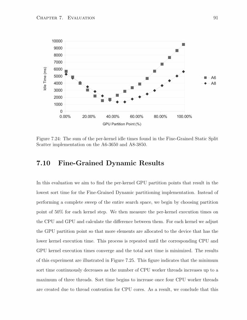
Chapter 7. Evaluation 91
0.00% 20.00% 40.00% 60.00% 80.00% 100.00%0
1000
2000
3000
4000
5000
6000
7000
8000
9000
10000
A6
A8
GPU Partition Point (%)
Idle
Tim
e (
ms)
Figure 7.24: The sum of the per-kernel idle times found in the Fine-Grained Static SplitScatter implementation on the A6-3650 and A8-3850.
7.10 Fine-Grained Dynamic Results
In this evaluation we aim to find the per-kernel GPU partition points that result in the
lowest sort time for the Fine-Grained Dynamic partitioning implementation. Instead of
performing a complete sweep of the entire search space, we begin by choosing partition
point of 50% for each kernel step. We then measure the per-kernel execution times on
the CPU and GPU and calculate the difference between them. For each kernel we adjust
the GPU partition point so that more elements are allocated to the device that has the
lower kernel execution time. This process is repeated until the corresponding CPU and
GPU kernel execution times converge and the total sort time is minimized. The results
of this experiment are illustrated in Figure 7.25. This figure indicates that the minimum
sort time continuously decreases as the number of CPU worker threads increases up to a
maximum of three threads. Sort time begins to increase once four CPU worker threads
are created due to thread contention for CPU cores. As a result, we conclude that this

Chapter 7. Evaluation 92
A6 A80
100020003000
4000500060007000
Fine Dynamic 1T
Fine Dynamic 2T
Fine Dynamic 3T
Fine Dynamic 4T
APU Model
Exe
cutio
n T
ime
(m
s)
Figure 7.25: The sort time of the Fine-Grained Dynamic partitioning implementationover a varying number of threads on the A6-3650 and the A8-3850
implementation does not scale well to four threads. This figure also indicates that the
minimum sort time for this implementation is lower on the A8-3850 than it is on the
A6-3650. This can be attributed to the different hardware characteristics of the two
platforms as discussed in Section 7.1.
The optimal per-kernel partition points for the Fine-Grained Dynamic implementa-
tion are provided in Table 7.2. For each kernel step, the value of the optimal partition
Optimal Partition Point
Kernel A6-3650 A8-3850
Local Sort 29 % 38 %Histogram 49 % 60 %Scatter 57 % 68 %
Table 7.2: Optimal per-kernel partition points for the Fine-Grained Dynamic implemen-tation.
point increases by approximately 10 percentage points when moving from the A6-3650 to
the A8-3850. This can once again be attributed to the different hardware characteristics
of the two platforms as discussed in Section 7.1.
We perform another experiment in order to understand how per-kernel partitioning
points affect the sort time of this implementation. We begin by setting all of the kernel
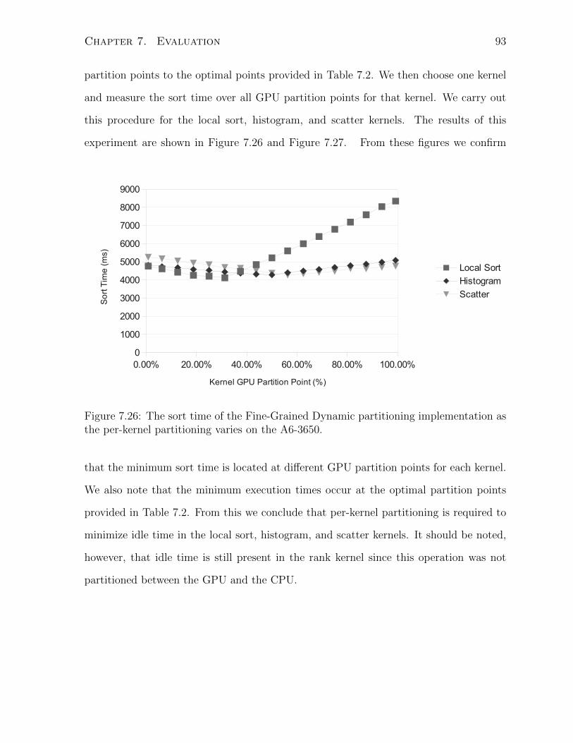
Chapter 7. Evaluation 93
partition points to the optimal points provided in Table 7.2. We then choose one kernel
and measure the sort time over all GPU partition points for that kernel. We carry out
this procedure for the local sort, histogram, and scatter kernels. The results of this
experiment are shown in Figure 7.26 and Figure 7.27. From these figures we confirm
0.00% 20.00% 40.00% 60.00% 80.00% 100.00%0
1000
2000
3000
4000
5000
6000
7000
8000
9000
Local Sort
Histogram
Scatter
Kernel GPU Partition Point (%)
So
rt T
ime
(m
s)
Figure 7.26: The sort time of the Fine-Grained Dynamic partitioning implementation asthe per-kernel partitioning varies on the A6-3650.
that the minimum sort time is located at different GPU partition points for each kernel.
We also note that the minimum execution times occur at the optimal partition points
provided in Table 7.2. From this we conclude that per-kernel partitioning is required to
minimize idle time in the local sort, histogram, and scatter kernels. It should be noted,
however, that idle time is still present in the rank kernel since this operation was not
partitioned between the GPU and the CPU.
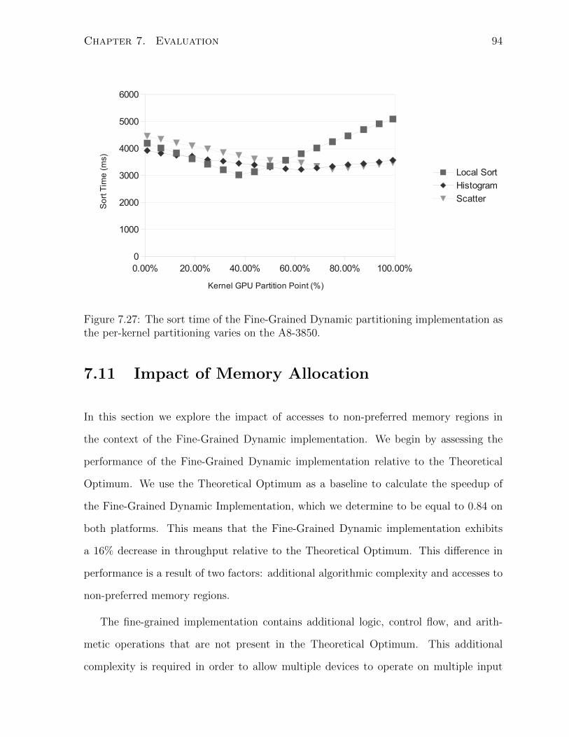
Chapter 7. Evaluation 94
0.00% 20.00% 40.00% 60.00% 80.00% 100.00%0
1000
2000
3000
4000
5000
6000
Local Sort
Histogram
Scatter
Kernel GPU Partition Point (%)
So
rt T
ime
(m
s)
Figure 7.27: The sort time of the Fine-Grained Dynamic partitioning implementation asthe per-kernel partitioning varies on the A8-3850.
7.11 Impact of Memory Allocation
In this section we explore the impact of accesses to non-preferred memory regions in
the context of the Fine-Grained Dynamic implementation. We begin by assessing the
performance of the Fine-Grained Dynamic implementation relative to the Theoretical
Optimum. We use the Theoretical Optimum as a baseline to calculate the speedup of
the Fine-Grained Dynamic Implementation, which we determine to be equal to 0.84 on
both platforms. This means that the Fine-Grained Dynamic implementation exhibits
a 16% decrease in throughput relative to the Theoretical Optimum. This difference in
performance is a result of two factors: additional algorithmic complexity and accesses to
non-preferred memory regions.
The fine-grained implementation contains additional logic, control flow, and arith-
metic operations that are not present in the Theoretical Optimum. This additional
complexity is required in order to allow multiple devices to operate on multiple input
Chapter 7. Evaluation 95
and output buffers simultaneously. Before we can assess the impact of memory allocation
on the Fine-Grained Dynamic implementation, we must first account for the performance
that is lost as a result of this additional algorithmic complexity.
We quantify the impact of additional algorithmic complexity in the Fine-Grained
Dynamic implementation by eliminating accesses to non-preferred memory regions. We
begin by measuring the additional complexity that is present in the GPU kernels. We
do this by measuring the sort time of the Fine-Grained Dynamic implementation with
the entire workload allocated to the GPU.1 This causes data to reside in uncached mem-
ory and effectively eliminates GPU accesses to cached memory.2 We then calculate the
speedup of this execution using the GPU-Only implementation as a baseline. We reason
that any difference in performance between this execution and the GPU-Only implemen-
tation is a result of the aforementioned algorithmic complexity in the GPU kernels.
We perform a similar test for the CPU kernels. We first measure the sort time
of the Fine-Grained Dynamic implementation with the entire workload allocated to the
CPU.3 This causes data to reside in cached memory, thereby eliminating CPU accesses to
uncached memory. We then calculate the speedup of this execution using the CPU-Only
implementation as a baseline. We reason that any difference in performance between
this execution and the CPU-Only implementation is a result of additional algorithmic
complexity in the CPU kernels.
The results of these experiments are presented in Figure 7.28. The experiments were
run using a total of 128 Mi elements with three CPU worker threads. The GPU speedups
are 0.97 and 0.99 on the A6-3650 and A8-3850, respectively. This means that the GPU
kernels exhibit a 3% decrease in throughput on the A6-3650 and a 1% decrease in through-
put on the A8-3850 relative to the GPU-Only implementation. The CPU speedups are
1The Fine-Grained Dynamic implementation requires that some work be assigned to each device. Wetherefore actually allocate 99% of the workload to the GPU.
2The counters and countersSum buffers remain cached since the CPU carries out the rank operation.3The Fine-Grained Dynamic implementation requires that some work be assigned to each device. We
therefore actually allocate 1% of the workload to the GPU.
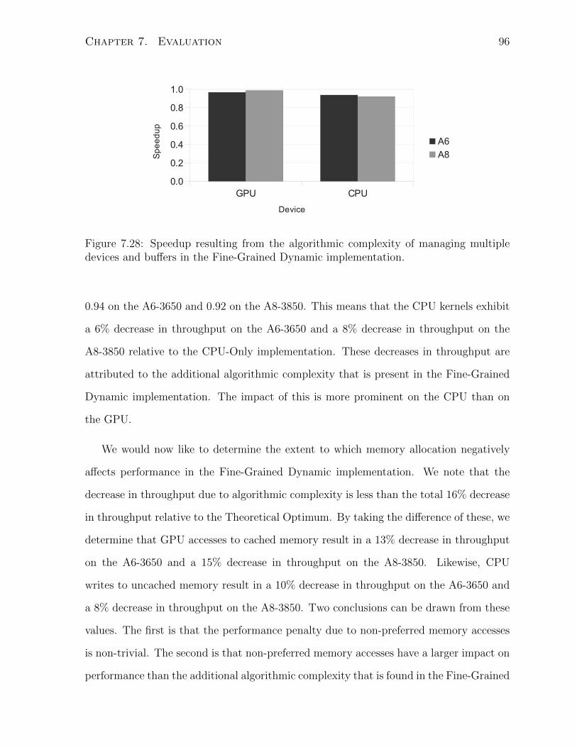
Chapter 7. Evaluation 96
GPU CPU0.0
0.2
0.4
0.6
0.8
1.0
A6
A8
Device
Speedup
Figure 7.28: Speedup resulting from the algorithmic complexity of managing multipledevices and buffers in the Fine-Grained Dynamic implementation.
0.94 on the A6-3650 and 0.92 on the A8-3850. This means that the CPU kernels exhibit
a 6% decrease in throughput on the A6-3650 and a 8% decrease in throughput on the
A8-3850 relative to the CPU-Only implementation. These decreases in throughput are
attributed to the additional algorithmic complexity that is present in the Fine-Grained
Dynamic implementation. The impact of this is more prominent on the CPU than on
the GPU.
We would now like to determine the extent to which memory allocation negatively
affects performance in the Fine-Grained Dynamic implementation. We note that the
decrease in throughput due to algorithmic complexity is less than the total 16% decrease
in throughput relative to the Theoretical Optimum. By taking the difference of these, we
determine that GPU accesses to cached memory result in a 13% decrease in throughput
on the A6-3650 and a 15% decrease in throughput on the A8-3850. Likewise, CPU
writes to uncached memory result in a 10% decrease in throughput on the A6-3650 and
a 8% decrease in throughput on the A8-3850. Two conclusions can be drawn from these
values. The first is that the performance penalty due to non-preferred memory accesses
is non-trivial. The second is that non-preferred memory accesses have a larger impact on
performance than the additional algorithmic complexity that is found in the Fine-Grained

Chapter 7. Evaluation 97
Dynamic implementation.
While the overhead of non-preferred memory accesses does impact the performance of
our Fine-Grained Dynamic implementation, we believe that we have carefully allocated
memory a way such that this impact is minimized. To illustrate this, we compare our
memory allocation strategy to two naive allocation strategies. We begin by measuring
the sort time of the Fine-Grained Dynamic implementation using our proposed memory
allocation strategy, which is described in Section 6.6. This sort time will be used as a
baseline to measure the speedup of subsequent allocation strategies. We then modify the
implementation such that all data is allocated in uncached host memory and calculate
the speedup. Finally, we calculate the speedup of the implementation with all buffers
completely allocated in cached host memory. This experiment was carried out on 128
Mi elements using three CPU worker threads. The optimal partition points in Table 7.2
were used for all allocation strategies. The results of this experiment are illustrated in
Figure 7.29. Allocating all buffers in uncached host memory results in a speedup of 0.05
Uncached Host Memory Cached Host Memory0
0.2
0.4
0.6
0.8
1
A6
A8
Memory Region
Sp
ee
du
p
Figure 7.29: Speedup resulting from alternate memory allocation strategies in the Fine-Grained Dynamic implementation.
on both the A6-3650 and the A8-3850. Placing everything in cached host memory results
in a speedup of 0.88 on the A6-3650 and 0.87 on the A8-3850.
We observe that allocating all buffers in uncached host memory has a very negative
Chapter 7. Evaluation 98
impact on performance. This is expected since CPU reads from uncached memory are
very slow, as described in Section 2.2.2. In contrast, our proposed allocation strategy
ensures that the CPU only accesses uncached memory in the form of streaming writes.
This makes efficient use of the on-chip write combining buffers and minimizes the impact
of CPU accesses to non-preferred memory regions.
Allocating all buffers in cached host memory also negatively impacts performance,
however to a lesser extent than allocating everything in uncached memory. Our proposed
allocation strategy reduces this penalty by reducing the number of GPU accesses to
cached memory. We conclude that one must carefully consider in which region to allocate
memory when designing algorithms for the AMD Fusion APU.
7.12 Comparative Performance
We compare each of the aforementioned implementations to one another in order to assess
their relative performance. We also compare them to the NVIDIA reference implementa-
tion and to the measured theoretical optimum implementation described in Section 6.7.
We do this by calculating the throughput of these implementations based on their re-
spective minimum sort times. For all implementations except for the NVIDIA reference,
these results are based on an input dataset size of 128 Mi elements. The results of the
NVIDIA reference implementation are based on an input dataset size of 4 Mi elements
due to the limitations described in Section 7.5. The throughputs of all implementations
are presented in Figure 7.30. These throughputs are not sensitive to the actual input
values,4 a result of sorting from least to most significant digits in radix sort. From this
figure we note that the NVIDIA reference and GPU-Only implementations have the low-
est throughput across both platforms. When the CPU-Only implementation is run with
three threads, it appears to perform similarly to the GPU-Only implementation on the
4This was confirmed by sorting on an already sorted input dataset.

Chapter 7. Evaluation 99
NV
IDIA
GP
U-O
nly
CP
U-O
nly 3T
CP
U-O
nly 4T
Coarse 3T
Coarse 4T
Fine 3T
Fine 4T
Fine S
S 3T
Fine S
S 4T
Fine D
yn 3T
Fine D
yn 4T
Optim
um
0
10
20
30
40
50
60
A6
A8
Implementation
Th
rou
gh
pu
t (M
i Ele
me
nts
/s)
Figure 7.30: Maximum sorting throughput of each implementation on the A6-3650 andthe A8-3850.
A8-3850. This is not true, however, for the A6-3650. This can once again be attributed
to the difference in the relative performance of the CPU and GPU across APU models.
The Coarse-Grained implementation with three worker threads achieves a relatively
high throughput of 31.7 Mi elements/s on the A6-3650 and 40.7 Mi elements/s on the
A8-3850. This implementation has very few inter-device synchronization points. The
CPU’s dataset and intermediate buffers are allocated in cached host memory, thereby
allowing it to access this data at the highest possible rate. Similarly, the GPU’s dataset
and intermediate buffers are allocated in host-visible device memory, which is the memory
region that the GPU has the highest bandwidth to. These aspects all contribute to the
high throughput of the Coarse-Grained implementation.
The Fine-Grained Static partitioning implementation with three threads has a through-
put of 23.9 Mi elements/s on the A6-3650 and 27.3 Mi elements/s on the A8-3850, giving
it the lowest throughput of the implementations that make use of both the CPU and
the GPU. This throughput does increase in the Fine-Grained Static Split Scatter im-

Chapter 7. Evaluation 100
plementation, thereby confirming the hypothesis that a significant amount of idle time
was present during the scatter step in the Fine-Grained Static implementation. The
Fine-Grained Dynamic implementation has the highest throughput of the implemented
versions of radix sort. The Fine-Grained Dynamic implementation achieved a through-
put of 32.8 Mi elements/s on the A6-3650 and 43.6 Mi elements/s on the A8-3850. This
indicates that per-kernel partitioning is necessary to reduce idle time and lower overall
sort time.
The throughput of the Fine-Grained Dynamic implementation is lower than that of
the measured theoretical optimum, which is 39.0 Mi elements/s on the A6-3650 and
51.9 Mi elements/s on the A8-3850. This difference in performance is because the Fine-
Grained Dynamic implementation contains additional algorithmic complexity and ac-
cesses to non-preferred memory regions, as discussed in Section 7.11.
In Figure 7.31 we present the speedup of each implementation with respect to the
NVIDIA reference implementation. These speedups are relative to the NVIDIA reference
NV
IDIA
GP
U-O
nly
CP
U-O
nly 3T
CP
U-O
nly 4T
Coarse 3T
Coarse 4T
Fine 3T
Fine 4T
Fine S
S 3T
Fine S
S 4T
Fine D
yn 3T
Fine D
yn 4T
Optim
um
0
0.5
1
1.5
2
2.5
3
A6
A8
Implementation
Sp
ee
du
p
Figure 7.31: Speedup with respect to the NVIDIA reference implementation on the A6-3650 and the A8-3850.
Chapter 7. Evaluation 101
implementation on each respective platform. Note that the speedup of each implementa-
tion that utilizes the CPU is greater on the A6-3650 than the A8-3850. This is because
the difference in performance between the CPU and GPU is greater on the A6-3650
than it is on the A8-3850. From this we conclude that the aforementioned multi-device
implementations provide a larger benefit to the A6-3650 than the A8-3850.
Across both platforms, the Fine-Grained Dynamic implementation with three threads
achieved the highest speedup of 2.40 on the A6-3650 and 1.88 on the A8-3850. These
speedups were less than the measured theoretical optimum speedup of 2.86 on the A6-
3650 and 2.24 on the A8-3850. With a speedup of 1.74 on the A6-3650 and 1.18 on
the A8-3850, the Fine-Grained Static implementation provided the lowest speedup of
the multi-device implementations. This was due to the idle time caused by the loss of
parallelism between the CPU and GPU in the scatter step and the fact that per-kernel
partitioning was not used in this implementation.
Chapter 8
Related Work
Parallel sorting has been a topic of study since at least the late 1960’s when Batcher
presented his work on sorting networks [19]. This work describes odd-even merging
networks and bitonic sorting networks, both of which are comparison sorts that carry
out individual comparisons in parallel. Since then, there has been a large amount of
work in adapting parallel sorting algorithms for evolving computer hardware. Nassimi
and Sahni [34] have adapted Batcher’s work [19] for parallel computers that have mesh
interconnects. Francis and Mathieson [26] have developed parallel merging techniques
that are used to sort datasets on shared memory multiprocessors. Blelloch et al [21]
have presented work on parallel sorting algorithms and implementations for the SIMD
Connection Machine Supercomputer model CM-2. This work provides adaptations of
several well known sorting algorithms, including bitonic sort, radix sort, and sample
sort. These works are similar to ours in that they adapt sorting algorithms in order to
make efficient use of modern hardware. They differ from our work, however, in that they
target neither GPU nor heterogeneous systems.
GPUs have been used to carry out parallel sorting operations prior to the release
of OpenCL in 2008 [1] and CUDA in 2007 [11]. Kipfer and Westermann [29] provided
algorithms for sorting on GPUs in 2005 using a framework called pug. They describe
102
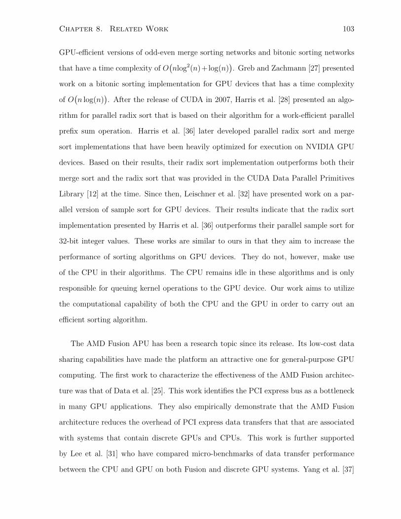
Chapter 8. Related Work 103
GPU-efficient versions of odd-even merge sorting networks and bitonic sorting networks
that have a time complexity of O(nlog2(n)+log(n)
). Greb and Zachmann [27] presented
work on a bitonic sorting implementation for GPU devices that has a time complexity
of O(n log(n)
). After the release of CUDA in 2007, Harris et al. [28] presented an algo-
rithm for parallel radix sort that is based on their algorithm for a work-efficient parallel
prefix sum operation. Harris et al. [36] later developed parallel radix sort and merge
sort implementations that have been heavily optimized for execution on NVIDIA GPU
devices. Based on their results, their radix sort implementation outperforms both their
merge sort and the radix sort that was provided in the CUDA Data Parallel Primitives
Library [12] at the time. Since then, Leischner et al. [32] have presented work on a par-
allel version of sample sort for GPU devices. Their results indicate that the radix sort
implementation presented by Harris et al. [36] outperforms their parallel sample sort for
32-bit integer values. These works are similar to ours in that they aim to increase the
performance of sorting algorithms on GPU devices. They do not, however, make use
of the CPU in their algorithms. The CPU remains idle in these algorithms and is only
responsible for queuing kernel operations to the GPU device. Our work aims to utilize
the computational capability of both the CPU and the GPU in order to carry out an
efficient sorting algorithm.
The AMD Fusion APU has been a research topic since its release. Its low-cost data
sharing capabilities have made the platform an attractive one for general-purpose GPU
computing. The first work to characterize the effectiveness of the AMD Fusion architec-
ture was that of Data et al. [25]. This work identifies the PCI express bus as a bottleneck
in many GPU applications. They also empirically demonstrate that the AMD Fusion
architecture reduces the overhead of PCI express data transfers that that are associated
with systems that contain discrete GPUs and CPUs. This work is further supported
by Lee et al. [31] who have compared micro-benchmarks of data transfer performance
between the CPU and GPU on both Fusion and discrete GPU systems. Yang et al. [37]
Chapter 8. Related Work 104
describe optimization techniques for a simulated fused CPU-GPU architecture similar to
Fusion. They recommend using the CPU to access data before it is required by the GPU,
thereby prefetching the data into the architecture’s shared L3 cache. They also simu-
late workload distribution between the GPU and GPU for several applications including
bitonic sort. They conclude that workload distribution between the GPU and CPU result
in a marginal improvement in performance and state that bitonic sort exhibits less than
a 2% performance improvement. These works are similar to ours in that they explore
the benefits of devices that contain both a GPU and CPU on a single chip. The works
of Data et al. [25] and Lee et al. [31] differ from ours in that they do not explore sorting
on these devices. While Yang et al. [37] do utilize bitonic sort in their benchmarks, they
focus on using the CPU to prefetch data for the GPU and conclude that the benefits of
workload partitioning are minimal. In contrast, we adopt the notion of workload parti-
tion and demonstrate that it can provide significant benefits in the context of sorting on
the AMD Fusion APU.
Chapter 9
Conclusions and Future Work
In this thesis, we have presented several radix sort algorithms that are designed to utilize
both the GPU and CPU components of the AMD Fusion APU. These algorithms were
implemented and evaluated on two APU models. Our results demonstrate that both
coarse-grained and fine-grained data sharing approaches outperform the current state of
the art GPU radix sort from NVIDIA [36] when executed on the AMD Fusion APU. We
therefore conclude that it is possible to efficiently use the CPU to speed up radix sort on
the Fusion APU.
We have found that fine-grained data sharing models can result in higher performance
than coarse-grained data sharing models on the AMD Fusion APU. This is only true,
however, if we redistribute data between the GPU and CPU at each algorithmic step
This is due to the fact that different computing architectures are inherently better suited
for certain types of tasks. Choosing a static partition point across all kernels results
in workload imbalance between the CPU and GPU at the per-kernel level. Per-kernel
data partitioning addresses this at the cost of increased algorithmic complexity and more
frequent accesses to non-preferred memory regions.
We have demonstrated the importance of carefully choosing the memory region in
which data is allocated on the Fusion APU. As discussed in Section 7.11, accessing data
105

Chapter 9. Conclusions and Future Work 106
in a non-preferred memory region can be detrimental performance. It is, however, often
necessary to do so as a means of providing fine-grained data sharing between the GPU
and CPU. We have provided memory allocation strategies for each of our algorithms that
minimize this performance impact.
The assessed combination of hardware and software does not allow the programmer
to change the memory region or caching designation of an allocated memory buffer.
We believe that this feature has the potential to speed up applications by reducing the
number of accesses that the GPU and CPU make to non-preferred memory regions. We
therefore make the recommendation this feature be integrated into future releases of the
hardware and software.
While the AMD Fusion APU hardware does allow for data buffers to be made available
to the GPU and CPU simultaneously, the OpenCL specification does not. The OpenCL
specification states that mapping a data buffer to the host and subsequently accessing it
from both the host and device simultaneously results in undefined behaviour. However,
the number of architectures that incorporate an on-chip GPU and CPU is increasing, and
as a result we recommend that the OpenCL specification incorporate a means of querying
whether data buffers can be safely accessed by the host and device simultaneously.
9.1 Future Work
The work presented in this thesis can be expanded by considering non-data parallel
models. The work in this thesis extends the data parallel approach presented by Satish
et al. [36] so that multiple devices may participate in the sort simultaneously. Instead,
a task parallel approach could be explored in which individual kernel steps are assigned
to certain devices.
The work in this thesis focused solely on the AMD Fusion APU. The scope of this
work may be expanded to include other architectures such as the recently released Intel
Chapter 9. Conclusions and Future Work 107
Ivy Bridge processor [14, 16], which also combines a GPU and CPU onto a single die.
Likewise, the research could be extended to include other sorting algorithms or even other
applications.
This research could be extended to also explore the Coarse-Grained implementation
of Fusion Sort on discrete graphics engines. The GPUs on such systems are commonly
much more powerful than the ones that have been studied in this work. Running the
Coarse-Grained implementation on such a system only changes our results by shifting
the optimal partition point such that a larger percentage of work is allocated to the GPU
for processing.1
It is also possible to extend our implementations of Fusion Sort by using SSE instruc-
tions. We expect that doing so will only cause the optimal partition points to shift such
that more work is allocated to the CPU for processing. We do not believe that this will
have an impact to any of the conclusions that were drawn in this study.
All variants of Fusion Sort are based upon a radix sort that operates from least to
most significant digit. The reasons for this are twofold. The first reason for this is that
implementing a least to most significant digit radix sort allows us to break the unsorted
dataset into equally sized tiles that can be operated upon by individual CPU threads or
GPU work-groups. The size of these tiles are not dependant on the distribution of the
unsorted input data or the size of each radix bucket, which allows for load balancing to
be done relatively easily. The second reason for using a least to most significant radix
sort is because the reference NVIDIA GPU implementation of radix sort is done from
least to most significant digit. Implementing Fusion Sort in the same manner allows us
to draw fair comparisons between our implementation and the current state of the art
GPU implementation from NVIDIA. Nonetheless, it would be interesting to explore a
version of Fusion Sort that operates from most to least significant digit.
1This was verified by running the Coarse-Grained implementation on a system with a discrete AMDHD5870 graphics card.
Chapter 9. Conclusions and Future Work 108
Finally, the work in this thesis could be extended to develop a method of determining
the optimal GPU partition point p for each APU model. It may be possible to determine
p theoretically using the hardware characteristics of the APU. It may also be possible to
determine p using a training kernel that carries out one or more small micro-benchmarks
either during program compilation or just prior to sort execution.
Bibliography
[1] The OpenCL specification, version: 1.0. http://www.khronos.org/registry/cl/
specs/opencl-1.0.pdf, 2008.
[2] AMD accelerated parallel processing (APP) SDK — AMD developer central. http:
//developer.amd.com/sdks/amdappsdk/pages/default.aspx, 2011.
[3] AMD accelerated parallel processing OpenCLTM programming guide.
http://developer.amd.com/sdks/AMDAPPSDK/assets/AMD_Accelerated_
Parallel_Processing_OpenCL_Programming_Guide.pdf, 2011.
[4] APU 101: All about AMD FusionTM accelerated processing units. http://
developer.amd.com/assets/apu101.pdf, 2011.
[5] Desktop PCs with AMD accelerated processors. http://www.amd.com/us/
products/desktop/apu/mainstream/Pages/mainstream.aspx#6, 2011.
[6] Family 12h AMD A-series accelerated processor product data sheet. http:
//support.amd.com/us/Processor_TechDocs/49894_12h_A-Series_PDS.pdf,
2011.
[7] The OpenCL specification, version: 1.1. http://www.khronos.org/registry/cl/
specs/opencl-1.1.pdf, 2011.
[8] Software optimization guide for AMD family 10h and 12h processors. http://
support.amd.com/us/Processor_TechDocs/40546.pdf, 2011.
109
BIBLIOGRAPHY 110
[9] AMD APP SDK download archive — AMD developer central. http://developer.
amd.com/tools/hc/AMDAPPSDK/downloads/pages/AMDAPPSDKDownloadArchive.
aspx, 2012.
[10] CUDA toolkit 4.2 - archive — NVIDIA developer zone. http://developer.nvidia.
com/cuda/cuda-toolkit-42-archive, 2012.
[11] CUDA toolkit archive — NVIDIA developer zone. https://developer.nvidia.
com/cuda-toolkit-archive, 2012.
[12] cudpp - CUDA data parallel primitives library - google project hosting. http:
//gpgpu.org/developer/cudpp, 2012.
[13] Intel R© many integrated core architecture - advanced. http://www.intel.com/
content/www/us/en/architecture-and-technology/many-integrated-core/
intel-many-integrated-core-architecture.html, 2012.
[14] Intel R© SDK for OpenCL applications 2012. http://software.intel.com/sites/
products/vcsource/files/43384/intel_sdk_for_ocl_2012_product_brief.
pdf, 2012.
[15] Previous catalystTM drivers. http://support.amd.com/us/gpudownload/
windows/previous/Pages/radeonaiw_vista64.aspx, 2012.
[16] Product brief: 3rd generation Intel R© CoreTM desktop prod-
uct brief. http://www.intel.com/content/www/us/en/research/
intel-labs-single-chip-cloud-computer.html, 2012.
[17] Single-chip cloud computer: Project. http://www.intel.com/content/www/us/
en/research/intel-labs-single-chip-cloud-computer.html, 2012.
BIBLIOGRAPHY 111
[18] G. Amdahl. Validity of the single processor approach to achieving large scale com-
puting capabilities. In Proceedings of the April 18-20, 1967, spring joint computer
conference, AFIPS ’67 (Spring), pages 483–485, New York, NY, USA, 1967. ACM.
[19] K. Batcher. Sorting networks and their applications. pages 307–314, 1968.
[20] G. Blelloch. Vector Models for Data-Parallel Computing (Artificial Intelligence).
The MIT Press, 1st edition edition, 1990.
[21] G. Blelloch, C. Leiserson, B. Maggs, C. Plaxton, S. Smith, and M. Zagha. A com-
parison of sorting algorithms for the connection machine CM-2. pages 3–16, 1991.
[22] P. Boulder and G. Sellers. Memory system on Fusion APUs: The benefits
of zero copy. http://developer.amd.com/afds/assets/presentations/1004_
final.pdf, 2011.
[23] N. Brookwood. AMD white paper: AMD FusionTM family of APUs: Enabling a su-
perior, immersive PC experience. http://sites.amd.com/us/documents/48423b_
fusion_whitepaper_web.pdf, 2010.
[24] T. Cormen, C. Leiserson, R. Rivest, and C. Stein. Introduction to Algorithms.
McGraw-Hill Science/Engineering/Math, 2nd edition, 2003.
[25] M. Daga, A Aji, and W. Feng. On the efficacy of a fused CPU+GPU processor
(or APU) for parallel computing. In Application Accelerators in High-Performance
Computing (SAAHPC), 2011 Symposium on, pages 141 –149, july 2011.
[26] R. Francis and I. Mathieson. A benchmark parallel sort for shared memory multi-
processors. Computers, IEEE Transactions on, 37(12):1619 – 1626, dec 1988.
[27] A. Greb and G. Zachmann. GPU-ABiSort: optimal parallel sorting on stream ar-
chitectures. In Parallel and Distributed Processing Symposium, 2006. IPDPS 2006.
20th International, page 10 pp., april 2006.
BIBLIOGRAPHY 112
[28] M. Harris, S. Sengupta, and J. Owens. Parallel prefix sum (scan) with CUDA. In
Hubert Nguyen, editor, GPU Gems 3, chapter 39, pages 851–876. Addison Wesley,
August 2007.
[29] P. Kipfer and R. Westermann. Improved GPU sorting. In Matt Pharr, editor, GPU
Gems 2, chapter 46. Addison Wesley, March 2005.
[30] D. Kirk and W. Hwu. Programming Massively Parallel Processors: A Hands-on
Approach. Morgan Kaufmann Publishers Inc., San Francisco, CA, USA, 1st edition,
2010.
[31] K. Lee, H. Lin, and W. Feng. Poster: characterizing the impact of memory-access
techniques on AMD fusion. In Proceedings of the 2011 companion on High Perfor-
mance Computing Networking, Storage and Analysis Companion, SC ’11 Compan-
ion, pages 75–76, New York, NY, USA, 2011. ACM.
[32] N. Leischner, V. Osipov, and P. Sanders. GPU sample sort. In Parallel Distributed
Processing (IPDPS), 2010 IEEE International Symposium on, pages 1 –10, april
2010.
[33] A. Munshi, B. Gaster, T. Mattson, J. Fung, and D. Ginsburg. OpenCL Programming
Guide. Addison-Wesley Professional, 1 edition, 2011.
[34] D. Nassimi and S. Sahni. Bitonic sort on a mesh-connected parallel computer.
Computers, IEEE Transactions on, C-28(1):2 –7, jan. 1979.
[35] N. Satish, M. Harris, and M. Garland. Designing efficient sorting algorithms for
manycore GPUs. NVIDIA Technical Report NVR-2008-001, NVIDIA Corporation,
2008.
[36] N. Satish, M. Harris, and M. Garland. Designing efficient sorting algorithms for
BIBLIOGRAPHY 113
manycore GPUs. In Parallel Distributed Processing, 2009. IPDPS 2009. IEEE In-
ternational Symposium on, pages 1 –10, may 2009.
[37] Y. Yang, P. Xiang, M. Mantor, and H. Zhou. CPU-assisted GPGPU on fused CPU-
GPU architectures. In High Performance Computer Architecture (HPCA), 2012
IEEE 18th International Symposium on, pages 1 –12, feb. 2012.
[38] K. Yoshida. Floating-point recurring rational arithmetic system. In T. Rao and
P. Kornerup, editors, IEEE Symposium on Computer Arithmetic, pages 194–200.
IEEE, 1983.


![HIP Coding · 2020. 12. 7. · 3 HIP Coding | ROCm Tutorial | AMD 2020 [AMD Official Use Only - Internal Distribution Only] Introduction 3 The Heterogeneous Interface for Portability](https://img.pdfslide.net/doc/110x75/60c6ea2958cdfa3d5944e2a2/hip-coding-2020-12-7-3-hip-coding-rocm-tutorial-amd-2020-amd-official.jpg)