Parallelization of the Kalman filter for multi-output systems on

UPTEC F12 025

Examensarbete 30 hpDecember 2012

Parallelization of the Kalman filter for multi-output systems on multicore platforms

Per Jonsson

Teknisk- naturvetenskaplig fakultet UTH-enheten Besöksadress: Ångströmlaboratoriet Lägerhyddsvägen 1 Hus 4, Plan 0 Postadress: Box 536 751 21 Uppsala Telefon: 018 – 471 30 03 Telefax: 018 – 471 30 00 Hemsida: http://www.teknat.uu.se/student

Abstract

Parallelization of the Kalman filter for multi-outputsystems on multicore platforms

Per Jonsson

The Kalman filter is a very commonly used signal processing tool for estimating statevariables from noisy observations in linear systems. Because of its cubic complexity, itis motivated to search for more computationally efficient Kalman filterimplementations.

In this thesis work, previous attempts of parallelizing the Kalman filter have beeninvestigated to determine whether any of them could run efficiently on modernmulti-core computers. Two of the most interesting methods from a multi-coreperspective have undergone further analysis to study how they perform in amulti-core environment. In the analysis, both state estimation accuracy and algorithmspeedup have been considered.

The experiment results indicate that one of the evaluated algorithms, denoted theFusion Gain method in this report, is faster on a quad-core CPU than astraight-forward implementation of the original Kalman filter when the number ofoutput signals is large. It should be noted, however, that this algorithm is not identicalto the true Kalman filter due to an approximation used in the derivation of themethod. Despite this detail, it might still be of use in some applications where speed ismore important than accurate state estimates.

The other evaluated method is based upon a fast Givens rotation. It was originallyimplemented on a so-called systolic array, which makes use of parallelism differentlythan multi-core computers. Unfortunately, this algorithm turned out to run very slowin the benchmarks even though the number of floating-point operations per second(FLOPS) should be far less than many of the other methods according to thetheoretical analysis. More attention could be devoted to this implementation to locatepossible bottlenecks.

ISSN: 1401-5757, UPTEC F12 025Examinator: Tomas NybergÄmnesgranskare: Kristiaan PelckmansHandledare: Alexander Medvedev

Contents

1 Introduction 5

1.1 Background . . . . . . . . . . . . . . . . . . . . . . . . . . . . . . . . . . . . . . . . . . . 5

1.2 The Thesis Work . . . . . . . . . . . . . . . . . . . . . . . . . . . . . . . . . . . . . . . . 6

2 Theory 6

2.1 The Kalman Filter . . . . . . . . . . . . . . . . . . . . . . . . . . . . . . . . . . . . . . . 6

2.2 Multi-Core Computers . . . . . . . . . . . . . . . . . . . . . . . . . . . . . . . . . . . . . 8

3 Existing Parallelization Approaches 10

3.1 Full-Order Distributed Kalman Filters . . . . . . . . . . . . . . . . . . . . . . . . . . . . 10

3.1.1 A Globally Optimal Method . . . . . . . . . . . . . . . . . . . . . . . . . . . . . 11

3.1.2 A Globally Sub-Optimal Method . . . . . . . . . . . . . . . . . . . . . . . . . . . 13

3.2 Reduced-Order Distributed Kalman Filters . . . . . . . . . . . . . . . . . . . . . . . . . 15

3.3 The Kalman Filter on Systolic Arrays . . . . . . . . . . . . . . . . . . . . . . . . . . . . 17

3.3.1 SIMD Arrays . . . . . . . . . . . . . . . . . . . . . . . . . . . . . . . . . . . . . . 18

3.3.2 Warp . . . . . . . . . . . . . . . . . . . . . . . . . . . . . . . . . . . . . . . . . . 20

3.3.3 Decoupling of Time-Update and Measurement-Update Equations . . . . . . . . . 21

4 Choice of System 22

4.1 A Temperature Bar . . . . . . . . . . . . . . . . . . . . . . . . . . . . . . . . . . . . . . . 23

5 Simulations 24

5.1 Setup . . . . . . . . . . . . . . . . . . . . . . . . . . . . . . . . . . . . . . . . . . . . . . 24

5.2 Experiments and Results . . . . . . . . . . . . . . . . . . . . . . . . . . . . . . . . . . . . 24

6 Algorithm Analysis 28

6.1 Fusion-Gain . . . . . . . . . . . . . . . . . . . . . . . . . . . . . . . . . . . . . . . . . . . 28

6.2 Fast-Givens Rotation . . . . . . . . . . . . . . . . . . . . . . . . . . . . . . . . . . . . . . 30

6.3 Summary . . . . . . . . . . . . . . . . . . . . . . . . . . . . . . . . . . . . . . . . . . . . 36

7 Implementation 38

7.1 Introduction . . . . . . . . . . . . . . . . . . . . . . . . . . . . . . . . . . . . . . . . . . . 38

7.2 The Algorithms . . . . . . . . . . . . . . . . . . . . . . . . . . . . . . . . . . . . . . . . . 38

7.2.1 Fusion-Gain . . . . . . . . . . . . . . . . . . . . . . . . . . . . . . . . . . . . . . . 38

7.2.2 Fast Givens Rotation . . . . . . . . . . . . . . . . . . . . . . . . . . . . . . . . . . 40

7.3 The Benchmark Software . . . . . . . . . . . . . . . . . . . . . . . . . . . . . . . . . . . 40

3

8 Preparations for the Final Run 41

8.1 Setting up the Test Cases . . . . . . . . . . . . . . . . . . . . . . . . . . . . . . . . . . . 41

8.2 Computer Environment . . . . . . . . . . . . . . . . . . . . . . . . . . . . . . . . . . . . 41

9 Final Results 42

9.1 Fusion Gain . . . . . . . . . . . . . . . . . . . . . . . . . . . . . . . . . . . . . . . . . . . 42

9.2 Fast Givens . . . . . . . . . . . . . . . . . . . . . . . . . . . . . . . . . . . . . . . . . . . 44

9.3 Experimental versus Predicted Results . . . . . . . . . . . . . . . . . . . . . . . . . . . . 44

9.4 Intel MKL with Thread Support Enabled . . . . . . . . . . . . . . . . . . . . . . . . . . 48

10 Discussion 50

10.1 Conclusions . . . . . . . . . . . . . . . . . . . . . . . . . . . . . . . . . . . . . . . . . . . 50

10.2 Future Work . . . . . . . . . . . . . . . . . . . . . . . . . . . . . . . . . . . . . . . . . . 51

4

1 Introduction

1.1 Background

The Kalman Filter In many technical applications there is a need to determine the state of somesystem of interest. For instance, in navigation or tracking applications it might be desirable to knowthe position and the speed of a vehicle. This can be accomplished by constructing a model of thesystem in terms of differential equations. The model reflects the dynamics of the system and how theinner state variables relate to the sensor measurements and the input to the system. Given this model,a well-known and widely used algorithm exists that fuses this information together to yield a stateestimate, namely the Kalman filter.

The Kalman filter was invented by Rudolf E. Kalman in 1960 (Kalman, 1960). It has since then beenwidely adopted, not only in technical applications, but also in other fields such as economics. Thefirst known implementation of the filter was in the navigation system used by the lunar module inthe Apollo 11 space mission, carried out by NASA in 1969. During the time when that project tookplace, many other techniques were also invented (Mcgee, 1985), e.g. the Extended Kalman filter, whichallowed nonlinear models to be used, and the Square-root implementation which greatly improved thenumerical stability of the implemented algorithm.

The filter consists of two parts. The first is the time-update step, in which the state vector is propagatedone discrete time-step using a model of the true system. The second part is the measurement-updatestep, which involves solving a Riccati equation and fusing its solution with measurement data toimprove the time-update prediction. The computational complexity of these steps is approximately ofthe order of O(n3

x) and O(n3z) respectively, where nx denotes the number of state variables and nz is

the number of measured output signals. Inevitably, the algorithm is quite demanding when it is appliedto large systems and could therefore be hard to apply, especially in real-time filtering applications.

The Entry of Multi-Core Computers Traditionally all central processing units (CPUs) on theconsumer market have only had one core. Due to a number of factors (mainly related to issues withhigher clock frequencies) it has become hard to achieve any significant performance gain using onlya single core. The remedy was to incorporate additional CPU cores on the same die, which makes itpossible to execute program code on multiple cores simultaneously. However, just adding an extra coredoes not automatically lead to a performance boost. To make the most of the multi-core architecture,the software has to be written in such way that it executes sections of code in parallel. How easy thisis to achieve depends on the specific situation. In a desktop environment it might be sufficient to runjust a small percentage of the work in parallel to make the computer seem more responsive. On theother hand, in the case with signal processing, it might be highly desirable to keep each CPU corefully utilized at all times.

The trend is that multi-core CPUs enter more and more areas and that the number of cores is increasing.Nowadays quad-core CPUs can even be found in handheld smart phone devices.

Previous Parallelization Attempts Since the time the Kalman filter was invented, various at-tempts have been made to enhance its computational performance. One of the first attempts datesback to 1976 when (Willner/Chang/Dunn, 1976) proposed a method for computing the Kalman filterwhen the sensors observing the system are located at different sites. The idea was to process eachsensor reading locally. If this was done simultaneously at each sensor computation time could hopefullybe saved. Papers along the same path include (Chong, 1979; Hashemipour/Roy/Laub, 1988; Carlson,1990; Paik/Oh, 2000). This category of Kalman filter parallelization techniques are referred to as“Distributed Kalman filter” and are covered in Section 3.1 and 3.2.

The other big category of parallel approaches are Kalman filters intended to run on so-called systolicarrays (Kung/Leiserson/of Computer Science, 1978). A systolic array is a signal processing resource

5

consisting of a number (often large) of simple processing elements connected together in a mesh-like structure. Data then “flows” through the array, one processing element at a time. This designturned out to be computationally efficient when performing common signal processing tasks, such asconvolutions and matrix multiplications. Attempts have been made to come up with Kalman filterimplementations that could run efficiently on systolic arrays (Gaston/Irwin, 1990). Many of themuse some form of square-root implementation. Some of them use Faddeev’s algorithm to perform thematrix operations, others use fast Givens rotations (Itzkowitz/Baheti, 1989; Palis/Krecker, 1990) andsome decouples the time-update equation from the measurement-update equation to process thosesimultaneously (Youmin et al., 1993).

1.2 The Thesis Work

The purpose of this thesis work is to investigate how ideas to parallelize the Kalman filter done in thepast (1960-) can be made to work on a modern multi-core architecture.

The strategy is to divide the work into smaller pieces. These are,

� Search for, and study publications done in the past to find out what approaches that are available.Summarize the findings. (Section 3)

� Decide what system to use for the simulations and benchmarks. (Section 4)

� Pick out a few methods to put under test. (Section 5)

� Simulate the system in Matlab and estimate the state using each of the picked out methods.(Section 5)

� Make reflections based on the result and possibly discard one or more of the methods that werenot good enough. (Section 5)

� Analyze the computation requirement of the remaining methods. (Section 6)

� Implement the methods in the C programming language and make them run on the super-computers at UPPMAX. (Section 7)

� Set up and run the final benchmarks at UPPMAX. Then present and comment on the result.(Section 9)

� Compare experimental performance with the theoretical predictions. (Section 9)

� Discuss the outcome of the entire thesis work. How did it go? What would be the next steps?(Section 10)

2 Theory

2.1 The Kalman Filter

The System Model Consider a model of a discrete dynamical system written on state-space form,

x(k + 1) = F (k)x(k) + Γ(k)u(k) +G(k)w(k) (2.1)

z(k) = H(k)x(k) + v(k) (2.2)

6

In this model the upper equation (2.1) describes the dynamics of the system expressed in terms of thestate variables contained in the state vector x(k). If the model would be an exact description of thetrue system the state transition matrix F (k) would completely describe the dynamics of the system.However, in most real-life applications this is not the case. This is why it is necessary to introducethe w(k) term, which is often referred to as the process noise. w(k) is a stochastic variable modeledas zero mean white Gaussian noise with the co-variance matrix Q(k).

The lower equation (2.2) is the so-called observation equation which tells us how the output vectorz(k) measurements are related to the internal state vector x(k). These readings are often affectedby a measurement noise v(k), which is here assumed to be zero mean white Gaussian noise with theco-variance matrix R(k).

All this can be expressed in mathematical notation as,

x(k) ∈ Rnx

u(k) ∈ Rnu

z(k) ∈ Rnz

w(k) ∈ Rnw

v(k) ∈ Rnz

F (k) ∈ Rnx×nx

Γ(k) ∈ Rnx×nu

G(k) ∈ Rnx×nw

H(k) ∈ Rnz×nx

w(k) ∼ N (0, Q(k))

v(k) ∼ N (0, R(k))

Q(k) ∈ Rnw×nw

R(k) ∈ Rnz×nz

The Discrete Kalman Filter What is needed to get hold of the state vector x(k) is an observer,such as the Kalman filter. It provides an optimal way of estimating the state variables of lineardynamical systems affected by white noise (w(k) and v(k)). An observer can be written as,

x(k + 1|k) = F (k)x(k|k − 1) + Γ(k)u(k) +K(k)ν(k)

ν(k) = z(k)−H(k)x(k|k − 1)

Here ν(k) is a measure of how well the model prediction corresponds to the measurement z(k), andis called the innovation or the residual. x(q|r) is the actual state estimate at time instant q basedon information from time sample 1 to r. The factor K(k) that minimizes the state estimate errorcovariance matrix P (k) is called the Kalman gain and can be expressed as,

K(k) = P (k|k − 1)HT (k)[H(k)P (k|k − 1)HT (k) +R(k)

]−1

P (k|k−1) denotes the so-called a priori state estimate error covariance for the a priori state estimatevector x(k|k − 1). k − 1 indicates that P (k|k − 1) and x(k|k − 1) are predictions based only oninformation available up to time sample k− 1. This is in contrast to the a posteriori estimates P (k|k)and x(k|k) which represent P (k) and x(k) when information from time sample k is used as well.

P (k|k − 1) = E[x(k|k − 1) · x(k|k − 1)T ]

P (k) = E[x(k|k) · x(k|k)T ]

x(k|k) = x(k)− x(k|k)

x(k|k − 1) = x(k)− x(k|k − 1)

7

The discrete Kalman filtering algorithm can be separated into two parts, namely the time-update stepand the measurement-update step. The time-update step is where the one-step prediction occurs,which tries to compute an a priori state estimate of the system’s state vector, one step ahead in time.In this step information about the dynamics of the model as described in (2.1) is used.

The second step is the measurement-update step in which the a priori estimate is “corrected” usinginformation from the sensor measurements.

The complete algorithm is presented in Algorithm 1.

Algorithm 1 The Kalman filter

Initialization:

x(−1| − 1) = xinitial guess

P (−1| − 1) = Pinitial guess

Time-update (a priori estimation):

x(k|k − 1) = F (k − 1)x(k − 1|k − 1) + Γ(k − 1)u(k − 1)

P (k|k − 1) = F (k − 1)P (k − 1|k − 1)FT (k − 1) +G(k − 1)Q(k − 1)GT (k − 1)

Measurement-update (a posteriori estimation):


]−1

x(k) = x(k|k − 1) +K(k) (z(k)−H(k)x(k|k − 1))

P (k) = [I −K(k)H(k)]P (k|k − 1)

Numerical Stability One problem with this straight-forward implementation (Algorithm 1) is therisk of numerical instability, which is prone to make the state error covariance matrix P non-positive-definite, and thus violating the Kalman filter requirement of P being postive-definite (Gustafsson,2000). This phenomena often occurs when the process error Q(k) is small. Other problems that mayhave bad influence on the numerical properties are e.g. the risk of P becoming asymmetric or loosingnumerical accuracy when the state variables are not scaled properly.

A way to overcome these issues is to work with a decomposition of the state error covariance P insteadof P itself. For instance, P could be decomposed as P = SST , where S is a matrix square root of P .This assures that P will not become non-positive-definite. To implement these ideas decompositiontechniques such as QR or LDLT are commonly used.

However, in this report Algorithm 1 is used when referring to the “Standard Kalman Filter” imple-mentation.

2.2 Multi-Core Computers

Parallel computing is about running two or more pieces of machine code simultaneously. The conceptis not new in any way, but has been used for decades in various forms. In recent years more attentionhas been devoted to the field of parallel computing (Faxen et al., 2008). The main cause for this isthe difficulties in gaining increased performance by increasing the CPU clock frequency. To overcomethis performance issue, CPU manufacturers have begun to implement different parallel strategies intotheir CPUs. One strategy is the Instruction Level Parallelism (ILP), where (independent) machineinstructions occurring close to each other in the program are run in parallel. This lowers the averagetime spent waiting for the CPU core when cache-misses occur.

8

RAM

L3

L2 L2 L2 L2

Core

1

Core

2

Core

3

Core

4

4x256 kB

8 MB

24 GB

Figure 2.1: Cache memory arrangement on a Intel Xeon Quad-core 5520 CPU (here with 24 GB ofexternal RAM).

Another approach is to put more than one core on the same chip, which is what multicore computingis all about. At this point there are basically two different paths to choose from. The first one is tohave a large number of quite primitive cores. This choice is often most suitable for problems where oneexpects the performance of the algorithm to grow with the number of cores, and is sometimes referredto as manycore. The second approach is to place a couple of standard CPU cores on the same chipand connect them together. We will concentrate on this type of platform, because it is was what wehave at our disposal for this thesis work.

The latter types of platforms are seen in the multicore CPUs found in today’s desktop and laptopcomputers, and recently even in smartphones. Similar kinds of CPUs are also found in the computationnetwork SNIC-UPPMAX (“Uppsala Multidisciplinary Center for Advanced Computational Science”).One example is the system Kalkyl at UPPMAX which consists of 348 computer nodes, where eachnode has two Intel Xeon Quad-core 5520 CPUs. Figure 2.1 shows the cache configuration and thememory sizes.

Programs that make use of the multicore architecture often use the OpenMP API to specify whatparts of the program should be run in parallel. OpenMP is fairly easy to use once you know how theprogram could be parallelized. Concluding how this could be made is the hard part.

There are a number of issues one should be aware of to succeed in the parallelization process. The goalwhen programming for multicores is to keep all the cores fully utilized. Things that will prevent youfrom accomplishing this are mainly slow memory, too much overhead and programming errors such asdeadlocks.

Cache The CPU cores operate at a much higher rate than the RAM memory. This is why the cachememories are so important. The cache memory is a memory placed between the CPU and the RAMmemory and acts as a fast, but small, buffer for the RAM. Without the cache memory the CPU corewould spend unreasonable amount of time waiting for data to be read (written) from (to) the RAMmemory.

On an ordinary single-core CPU there are most often one to three levels of cache memories betweenthe CPU and the RAM memory. The L1 cache is the fastest, but smallest, cache memory and sitsclosest to the CPU. The L3 cache, on the other hand, is the slowest, but largest cache memory.

On multi-core CPUs some of the cache memories are shared and some are not. A common cachememory arrangement could e.g. be as depicted in Figure 2.1, where each core has its own L2 cache.

What makes it into the cache usually follows the principles behind temporal locality and spatial locality,i.e. data that has recently been accessed is likely to be used again very soon and the neighboring dataas well. This also holds for single-core machines. What gets complicated in the multi-core case is to

9

Master thread

(thread 0)

Fork Join

Master thread

(thread 0)

Master thread

(thread 0)

thread 1

thread M-2

thread M-1

Figure 2.2: Fork-join model

maintain consistency among the individual caches. If one core alters the content of a memory locationthe rest of the caches holding the same bit of memory need to be updated to reflect the new state. Ofcourse, all this is handled by the hardware, but it is nevertheless good to be aware of in order to writeefficient code.

Overhead When attempting to parallelize an algorithm, the key is to find a section that is largeenough to be worth parallelizing. The reason for this is that the overhead associated with enteringand exiting a parallel section would otherwise become larger than the actual performance gain ofparallelizing that piece of code in the first place. The overhead comes from the time it takes tosplit the current program flow into a series of new threads and then, when the threads are finished,synchronize everything again. This is also known as the fork-join model. Figure 2.2 illustrates howthis works.

When the application is first started it is running in the master thread. Later, when the programexecution encounters a parallel section one or more additional threads are spawned. The operatingsystem can then choose to execute the threads in parallel on one or more available cores. When thethreads finish, a synchronization step takes place, where it is made sure that the memory is consistent.During this phase all threads, except for the master thread, will terminate.

3 Existing Parallelization Approaches

The outcome of this section lays the basis for the remaining parts of the work. The plan has been toskim through a number of papers to get an idea of existing solutions to parallelizing the Kalman filter.While reading the articles short notes have been written down that summarize the papers.

Then, every note has been sorted so that similar methods get into the same category. These categoriesturned out to be,

� Distributed filters

� Filter used on large computer arrays

� Decoupling of time-update and measurement-update

3.1 Full-Order Distributed Kalman Filters

The typical need for the distributed Kalman filter arises when several sensors, spread out geographicallyare used together to make observations on a common system. The sensor nodes are often connectedto a central computer that computes the global estimate of the system using the information receivedfrom the sensor nodes.

Also fault detection and correction are integrated in these methods, which often implies that the centralcomputer is able to get a state estimate even in situations where some of the local filter nodes for some

10

reason are unable to provide their local estimates to the global filter. Another possibility could beto exclude certain local state estimates from the global collating filter in cases where a sensor outputreports estimates that are clearly erroneous.

This idea of distributed computing could most certainly be applicable to multicore computers if thesensors are not assumed to be spread out geographically, but rather be connected to the same machine.The local sensor processing can then be carried out on different cores on the same CPU instead ofbeing computed at the spread out sensor nodes.

Over the years many different methods have been suggested that make use of the distributed approach,each with their own advantages and disadvantages. One of the first contributions was made in (Willner/Chang/Dunn, 1976). At each sensor node a local sequential Kalman filter is attempting to estimatethe global state vector at each sample period using sensor data only from that sensor. However, thesensor nodes are not entirely autonomous. In addition to the variables required to run a standardKalman filter it also requires the global estimate vector from the previous time step. When the localstate estimation vector and the corresponding covariance matrix have been computed, the result istransmitted to the central processor. The central processor then combines the information receivedfrom its child nodes to yield the global state estimate (see Figure 3.1).

Central computer

Sensor node 1 Sensor node 2 Sensor node N...

Figure 3.1: Two-way communication

3.1.1 A Globally Optimal Method

In the frequently cited paper (Hashemipour/Roy/Laub, 1988) a method similar to (Willner/Chang/Dunn, 1976) is proposed with the exception that the local filters do not need to know of the globalestimate. This means that each sensor only has to communicate with the central processor over aone-way communication link (see Figure 3.2) which can be beneficial especially when communicationis associated with significant performance costs.

Central computer

Sensor node 1 Sensor node 2 Sensor node N...

Figure 3.2: One-way communication

In (Hashemipour/Roy/Laub, 1988) different methods are suggested depending on whether the sensorsare positioned geographically close to each other or if delays can be expected due to the sensors beingspread out. The partitioning of the global system into the N local systems, in the case where thesensors are co-located, is done by dividing the observation vector into smaller sub-vectors, so that eachlocal model becomes,

x(k + 1) = F (k)x(k) + Γ(k)u(k) +G(k)w(k)

zj(k) = Hj(k)x(k) + vj(k)

11

where,

z(k) = [ zT1 (k) · · · zTN (k) ]T

H(k) = [ HT1 (k) · · · HT

N (k) ]T

v(k) = [ vT1 (k) · · · vTN (k) ]T

vj(k) ∈ Rmj ,

N∑j=1

mj = m

Furthermore, it is assumed that there is no correlation between any two sensor measurement noisesvj(k) or between the measurement noises vj(k) and the process noise w(k).

E{vj(k)vk(k)} = 0, j 6= k

E{v(k)w(k)} = 0

E{v(k)vT (k)} = block diag{R1, · · · , RN}E{w(k)wT (k)} = Q

The time-update and measurement-update equations to be computed at sensor node j, will have thesame form as a standard Kalman filter, see Algorithm 2.

Algorithm 2 Local filter (full-order)

Initialization:

xj(−1| − 1) = xinitial guess

Pj(−1| − 1) = Pinitial guess

Local time-update:

xj(k|k − 1) = F (k − 1)xj(k − 1|k − 1) + Γj(k − 1)uj(k − 1)

Pj(k|k − 1) = F (k − 1)Pj(k − 1|k − 1)FT (k − 1) +G(k − 1)Q(k − 1)GT (k − 1)

Qj(k − 1) = G(k − 1)[Q(k − 1)− (N − 1)/N Q(k − 1)

]GT (k − 1)

Local measurement-update:

Kj(k) = Pj(k|k − 1)HTj (k)

[Hj(k)Pj(k|k − 1)HT

j (k) +Rj(k)]−1

xj(k|k) = [I −Kj(k)Hj(k)] xj(k|k − 1) +Kjzj

Pj(k|k)−1 = Pj(k|k − 1)−1 +HTj (k)R−1

j (k)Hj(k)

Through a number of substitutions (Hashemipour/Roy/Laub, 1988) the expressions for the globaltime-update and global measurement-update can finally be obtained as seen in Algorithm 3.

12

Algorithm 3 Global filter (full-order)

Initialization:



Global time-update:

x(k|k − 1) = F (k − 1)x(k − 1|k − 1)− (N − 1)Γ(k − 1)u(k − 1)

P (k|k − 1) = F (k − 1)P (k − 1|k − 1)FT (k − 1) +G(k − 1)Q(k − 1)GT (k − 1) =

= F (k − 1)P (k − 1|k − 1)FT (k − 1) +

N∑j=1

Qj(k − 1)

Global measurement-update:

x(k|k) = P (k|k)

P (k|k − 1)−1x(k|k − 1) +

N∑j=1

HTj (k)R−1

j (k)zj(k)

=

= P (k|k)

[P (k|k − 1)−1x(k|k − 1) +

N∑j=1

{P (k|k)−1

j x(k|k)j − Pj(k|k − 1)−1xj(k|k − 1)} ]

P (k|k)−1 = P (k|k − 1)−1 +

N∑j=1

HTj (k)R−1

j (k)Hj(k) =

= P (k|k − 1)−1 +

N∑j=1

{P (k|k)−1

j − Pj(k|k − 1)−1}

Conclusions This method could be a candidate for implementation on a multicore machine. Eachof the N local filters could run on a separate core on a multicore computer. More than one filter couldpossibly be assigned to some of the cores if the number of cores is greater than N .

3.1.2 A Globally Sub-Optimal Method

Based on the prior work of e.g. (Hashemipour/Roy/Laub, 1988) and (Carlson, 1990) a new, sub-optimal composition of the distributed Kalman filter was developed in (Paik/Oh, 2000). The principlebehind the idea is to put an upper bound on the covariance of the residual of the global model, denotedS in the Kalman gain equation,

K(k + 1) = P (k + 1)HT (k + 1)S−1(k + 1) (3.1)

S(k + 1) = H(k + 1)P (k + 1|k)HT (k + 1) +R(k + 1)

It can be shown (e.g. (Carlson, 1990)) that S is upper-bounded by,

S(k + 1) ≤ block diag{γ1S1(k + 1), · · · , γNSN (k + 1)} (3.2)

where the local residuals are given by,

Sj(k + 1) = Hj(k + 1)Pj(k + 1|k)HTj (k + 1) + (1/γj)Rj(k + 1) (3.3)

13

and γj ≥ 1 are weights (normally γj = N , as mentioned in (Carlson, 1990)) applied locally to allowfusion of the local results to yield the global estimate.

Then by substituting S in (3.1) with the upper bound in (3.2), (3.1) can be parallelized through (3.3).This is also where the sub-optimality of this method is introduced. This makes it possible to write theKalman gains as,

K(k + 1) = P (k + 1|k)

[1

γ1HT

1 (k + 1)S−11 (k + 1), · · · , 1

γNHTN (k + 1)S−1

N (k + 1)

]Kj(k + 1) =

1

γjPj(k + 1|k)HT

j (k + 1)S−1j (k + 1)

The global error covariance (P (k|k)) and the global state estimate (x(k|k)) are given as Step 4 inAlgorithm 4. For expressing P (k|k) the author has chosen to use the so-called “Joseph stabilizedformula” to give a numerically more stable solution.

Algorithm 4 A sub-optimal distributed variant of the Kalman filter

Initialization:



1. Perform Global Time-Update:

x(k|k − 1) = F (k − 1)x(k − 1|k − 1) + Γ(k − 1)u(k − 1)

P (k|k − 1) = F (k − 1)P (k − 1|k − 1)FT (k − 1) +G(k − 1)Q(k − 1)GT (k − 1)

2. Assign the result to the local filters (j = 1, · · · , N) as well:

xj(k|k − 1) = x(k|k − 1)

Pj(k|k − 1) = P (k|k − 1)

3. On each local node compute the local Kalman gain and state estimates:

Kj(k) =1

γjP (k|k − 1)HT

j (k)

[Hj(k)P (k|k − 1)HT

j (k) +1

γjRj(k)

]−1

xj(k|k) = x(k|k − 1) +Kj(k) [zj(k)−Hj(k)x(k|k − 1)]

4. Perform the global fusion:

x(k|k) = (1−N)x(k|k − 1) +

N∑j=1

xj(k|k)

P (k|k) =

I − N∑j=1

Kj(k)Hj(k)

P (k|k − 1)

I − N∑j=1

Kj(k)Hj(k)

T +

+

N∑j=1

Kj(k)Rj(k)KTj (k)

Conclusions This is a sub-optimal filter, and hence not a “true” Kalman filter, with the advantageof possibly being more computationally efficient than the optimal variant. For instance, the absence

14

of computationally costly inversions in the global steps (Step 1 and Step 4 in Algorithm 4) might befavorable when being implemented on a multicore computer.

3.2 Reduced-Order Distributed Kalman Filters

In (Roy/Hashemi/Laub, 1991) a further developed variant of (Hashemipour/Roy/Laub, 1988) waspublished that uses local filters of reduced order. While the aim of this method is to achieve aglobally optimal state estimation, reduction of order is not always possible for an arbitrary system. Arequirement is that any state variable must not be part of more than one local filter. This implicatesthat the system matrix, F , needs to be block diagonal.

After performing the following derivation it turns out that the algorithm will look almost identical tothe algorithm proposed in (Hashemipour/Roy/Laub, 1988) except that this method requires the extra“translation matrices” Dj and Ej .

Again, consider the global system model,

x(k + 1) = F (k)x(k) +G(k)w(k)

z(k) = H(k)x(k) + v(k)

Let z, v, w, G and H be partitioned into N separate blocks as,

z(k) = [ zT1 (k) · · · zTN (k) ]T

w(k) = [ wT1 (k) · · · wTN (k) ]T

v(k) = [ vT1 (k) · · · vTN (k) ]T

H(k) = [ HT1 (k) · · · HT

N (k) ]T

G(k) = [ GT1 (k) · · · GTN (k) ]T

Then construct a local system model,

xj(k + 1) = Fj(k)xj(k) +G(r)j (k)wj(k)

zj(k) = H(r)j (k)xj(k) + vj(k)

Here G(r)j (k) ∈ Rnj×pj and H

(r)j (k) ∈ Rmj×nj denote the reduced-order process and measurement

noise matrices respectively, with∑Nj=1 pj = p and

∑Nj=1mj = m.

Fj(k) ∈ Rnj×nj is the reduced-order state transition matrix operating on the reduced-order statevector xj(k) ∈ Rnj .

It is obvious that Algorithm 3 is no longer valid under these new conditions, e.g. due to the possibledimension mismatch in the summation. However, if a matrix Dj(k) ∈ Rnj×n can be found such that,

Hj(k) = H(r)j (k)Dj(k)

and if there exists a matrix Ej(k) ∈ Rn×nj such that,

Gj(k) = Ej(k)G(r)j (k)

then Algorithm 3 can be rewritten as seen in Algorithm 5.

15

Algorithm 5 Global filter (reduced-order)

Initialization:



Global time-update:

x(k|k − 1) = F (k − 1)x(k − 1|k − 1)

P (k|k − 1) = F (k − 1)P (k − 1|k − 1)FT (k − 1) +N∑j=1

Ej(k − 1)[G

(r)j (k − 1)Qj(k − 1)G

(r)Tj (k − 1)

]ETj (k − 1)

= F (k − 1)P (k − 1|k − 1)FT (k − 1) +N∑j=1

Ej(k − 1)[Pj(k|k − 1)− Fj(k − 1)Pj(k|k)FTj (k − 1)

]ETj (k − 1)


x(k|k) = P (k|k)

P (k|k − 1)−1x(k|k − 1) +

N∑j=1

DTj (k)[H

(r)Tj (k)R−1

j (k)zj(k)]

=

= P (k|k)

[P (k|k − 1)−1x(k|k − 1) +

+

N∑j=1

DTj (k)

{Pj(k|k)−1x(k|k)j − Pj(k|k − 1)−1xj(k|k − 1)

} ]

P (k|k)−1 = P (k|k − 1)−1 +

N∑j=1

DTj

[H

(r)Tj (k)R−1

j (k)H(r)j (k)

]Dj(k) =

= P (k|k − 1)−1 +

N∑j=1

DTj (k)

{P (k|k)−1

j − Pj(k|k − 1)−1}Dj(k)

The algorithms to be executed locally will have the same form as before, as seen in Algorithm 6.

16

Algorithm 6 Local filter (reduced-order)

Initialization:

xj(−1| − 1) = xinitial guess

Pj(−1| − 1) = Pinitial guess

Global time-update:

xj(k|k − 1) = Fj(k − 1)xj(k − 1|k − 1)

Pj(k|k − 1) = Fj(k − 1)Pj(k − 1|k − 1)FTj (k − 1) +G(r)j (k − 1)Qj(k − 1)G

(r)Tj (k − 1)


Kj(k) = Pj(k|k − 1)H(r)Tj (k)

[H

(r)j (k)Pj(k|k − 1)H

(r)Tj (k) +Rj(k)

]−1

xj(k|k) =[I −Kj(k)H

(r)j (k)

]xj(k|k − 1) +Kj(k)zj(k)

Pj(k|k) =[I −Kj(k)H

(r)j (k)

]Pj(k|k − 1)

Conclusions Having a reduced-order model helps reducing the computation burden on each sensornode since fewer operations have to be performed. It also provides a solution to the problem wherenot all local filters can observe all state variables.

3.3 The Kalman Filter on Systolic Arrays

Apart from the more general methods of parallelizing the Kalman filter there has also been an ongoingresearch on how the Kalman filter can be computed efficiently on customized hardware architectures.The architecture in this field which perhaps has got the most attention in the past is the so-calledsystolic array.

The systolic array (Kung/Leiserson/of Computer Science, 1978; Hoffmann/Devadas/Agarwal, 2010)consists of a big one- or two-dimensional array of simple data processing elements (PEs) (see Figure3.3). At every clock cycle each PE grabs a data element from the input data stream, processes it andthen passes it on to the next PE in the array. In addition to being able to perform simple operationseach PE can also be designed to have internal registers where intermediate results can be stored.

The concept is quite different from how the multicore architecture is designed. A multicore computertypically do not have nearly as many cores as the systolic array has PEs. On the systolic array noextra computational cost is associated with letting a PE perform just one operation. It would notbe beneficial to let a core in a multicore system perform one single operation due to the overheadassociated with loading and storing of the data and the synchronization handling.

However, there exists at least one recent attempt to convert existing systolic implementations to themulticore architecture. A method presented in (Vinjamuri/Prasanna, 2009) divides the entire systolicarray into larger groups of PEs. Those groups are named macro-nodes and the PEs that the macro-nodes are built up by are called micro-nodes.

To determine how the systolic array can be divided up into macro-nodes, it is necessary to know thedependency relations in the array. As mentioned earlier the data flows through the array, at the paceof one step per clock cycle. An important observation to make here is the case when some PEs do notalter the data before it is passed on to the neighboring PE. This means that the neighboring PE is notdependent on the result from the previous PE. This fact can be exploited when laying out the workon the different cores on the multicore computer.

17

Data input

Data input

Data output

Data output

PE PE PE PE

PE

PE

PEPE

PE

PEPE

PE

PEPE

PE

PE

Figure 3.3: Principle of a 2D systolic array

3.3.1 SIMD Arrays

Another architecture is the SIMD (“Single Instruction Multiple Data”) array. Just like with systolicarrays the SIMD array contains a large number of processing elements (PEs). One important differencethough is that the commands, that are to be executed synchronously on each PE, are issued by aControl unit instead of being “hardwired”. The data on which to perform the operations on is alreadystored in the local memories of the PEs on beforehand instead of being clocked in as in the case withthe systolic array.

The fact that a Control unit determines the behavior of the array at each clock cycle means thatthe approach taken in (Vinjamuri/Prasanna, 2009), to apply a systolic array design on a multicorecomputer, would possibly become much harder since the behavior of the array is no longer static.

A suggestion of an implementation on a commercially available SIMD array called “Connection Ma-chine” is presented in (Palis/Krecker, 1990). The method used is a Square-Root like variant of theKalman filter. What follows here is a very brief explanation of the method to give an idea of how animplementation on a SIMD array could look like.

Start with the well-known state-space representation of a system,

x(k + 1) = F (k)x(k) + Γ(k)u(k) +G(k)w(k)

z(k) = H(k)x(k) + v(k)

The matrices P (k) and Re(k) can be written in the factorized form,

P (k) = Lp(k)Dp(k)LTp (k)

Re(k) = Le(k)De(k)LTe (k)

where,

Re(k) = H(k)P (k)HT (k) +R(k)

P (k + 1) = F (k)P (k)FT (k) +G(k)Q(k)GT (k)−K(k)Re(k)KT (k)

Let S be the matrix,

S(k) =

[Re(k) H(k)P (k)FT (k)

F (k)P (k)HT (k) F (k)P (k)FT (k) +G(k)Q(k)GT (k)

]Then it can be shown that S can be factored as,

S(k) = A(k)D(k)AT (k) = (3.4)

=

[I H(k)Lp(k) 00 F (k)Lp(k) G(k)

] R(k) 0 00 Dp(k) 00 0 Q(k)

I 0LTp (k)HT (k) LTp (k)FT (k)

0 GT (k)

18

Alternatively, S can also be factored as,

S = A′(k)D′(k)A′T (k) = (3.5)

=

[Le(k) 0 0

K(k)Le(k) Lp(k + 1) 0

] De(k) 0 00 Dp(k + 1) 00 0 Da

LTe (k) LTe (k)KT (k)0 LTp (k + 1)0 0

To get from (3.4) to (3.5) one possibility is to use a triangularization algorithm like for instance the“fast Givens rotations”.

The complete scheme proposed in (Palis/Krecker, 1990) for performing the Kalman filtering is repli-cated in Algorithm 7.

Algorithm 7 Square-Root Kalman with fast Givens rotation

Input: xo, Lp,0, Dp,0, F (k), H(k), R(k), Q(k), G(k), z(k) for k ≥ 0Output: x(k) for k > 0Steps: For k = 0, 1, 2, · · · , do the following:

1. Set up matrices A and D such that:

A =


]and D =

R(k) 0 00 Dp(k) 00 0 Q(k)

2. Triangularize A to obtain:

A′ =

[Le(k) 0 0

K(k)Le(k) Lp(k + 1) 0

]and

D′ =

De(k) 0 00 Dp(k + 1) 00 0 Da

such that S = ADAT = A′D′A′T .

3. Compute K(k) [z(k)−H(k)x(k)] as follows:(a) Compute c(k) = z(k)−H(k)x(k)(b) Solve Le(k)s(k) = c(k) for s(k)(c) Compute K(k) [z(k)−H(k)x(k)] = [K(k)Le(k)] s(k)

4. Compute and output:x(k + 1) = F (k)x(k) + Γ(k)u(k) +K(k) [z(k)−H(k)x(k)]

In the paper focus is devoted to Step 2 in Algorithm 7 because it is concluded that it stands for 3/4of the total number of floating-point operations. Step 2 can be written in a pseudo programminglanguage as,

f o r q = (1 to M) dof o r j = ( q to N) do

(A,D) = Tqj (A,D)end

end

The parallelization strategy presented in the paper is then to parallelize the inner loop using a constantnumber of operations. Let A(q) and D(q) denote the matrices at the end of iteration q.

Then it can be shown that the elements in A and D can be computed as,

d(q)q = s

(q−1)qN and d

(q)j =

s(q−1)q,j−1

s(q−1)qj

d(q−1)j , q < j ≤ N

19

a(q)iq =

s(q−1)iN

s(q−1)qN

and a(q)ij = a

(q−1)ij − s

(q−1)i,j−1

s(q−1)q,j−1

a(q−1)qj , q ≤ i ≤M and q < j ≤ N

where,

s(q−1)ij =

∑jl=q a

(q−1)ql a

(q−1)il d

(q−1)l .

Thus the first (q− 1) diagonal elements in D(q) will be the same as in D(q−1) and the first (q− 1) rowsand the first (q − 1) columns of A(q) will be the same as in A(q−1).

The complete scheme for implementing the fast Givens rotation step is presented in Algorithm 8.Because this algorithm is aimed to run on a SIMD computer, which can be seen on the algorithmstructure, it is not clear if it could be useful for multicore computers.

Algorithm 8 Fast Givens rotation on a “Connection Machine”

Initialization: See the original paper (Palis/Krecker, 1990)

For q = 1, . . . ,M :

1. For all columns j, q ≤ j ≤ N , spread-with-copy a(q, j) down the column and store it in b(i, j),

q ≤ i ≤M . (Thus, b(i, j) = a(q−1)qj )

2. For q ≤ i ≤ M and q ≤ j ≤ N , compute t1(i, j) = a(i, j) · b(i, j) · d(i, j) (Thus, t1(i, j) =

a(q−1)ij a

(q−1)qj d

(q−1)j )

3. For all rows i, q ≤ i ≤ M , perform an upward, exclusive, scan-with-add over the set of values

{t1(i, j)|q ≤ j ≤ N + 1}. (Thus, t1(i, j) = s(q−1)i,j−1 )

4. For all columns j, q ≤ j ≤ N , spread-with-copy t1(q, j) down the column and store it in t2(i, j),

q ≤ i ≤M . (Thus, t2(i, j) = s(q−1)q,j−1)

5. For q ≤ i ≤ M and q < j ≤ N + 1, compute t1(i, j) = t1(i, j)/t2(i, j). (Thus, t1(i, j) =

s(q−1)i,j−1 /s

(q−1)q,j−1; in particular, t1(i,N + 1) = a

(q)iq and t2(i,N + 1) = d

(q)q )

6. For q ≤ i ≤ M , send t1(i,N + 1) to a(i, q) and send t2(i,N + 1) to d(i, q). (Thus, a(i, q) = a(q)iq

and d(i, q) = d(q)q )

7. For q ≤ i ≤M and q < j ≤ N , compute a(i, j) = a(i, j)− b(i, j) · t1(i, j). (Thus, a(i, j) = a(q)ij )

8. For q ≤ i ≤ M and q < j ≤ N , get t1(i, j) from t2(i, j + 1). (Thus, t1(i, j) = s(q−1)qj and

t2(i, j) = s(q−1)q,j−1)

9. For q ≤ i ≤M and q < j ≤ N , compute d(i, j) = d(i, j) · t2(i, j)/t1(i, j). (Thus, d(i, j) = d(q)j )

3.3.2 Warp

Another method which is based on the same Square-Root Kalman filter, using the same decompositiontechnique, is found in (Itzkowitz/Baheti, 1989). In the paper an algorithm designed to run on a Warpcomputer (Kung, 1984) is proposed.

The Warp architecture is a hardware implementation of a systolic array originating from 1984. EachPE has its own pipelined multiplier and ALU (“Arithmetic Logic Unit”), and has also access to a smallprivate RAM. This makes it slightly more advanced and versatile than many other systolic arrays. ThePEs are interconnected via a 1D array.

In (Itzkowitz/Baheti, 1989) the implementation of the triangularization step (Step 2 in Algorithm 7)is instead described by Algorithm 9.

20

Algorithm 9 A Fast Givens rotation

For each row Ai in A (i = 1, · · · ,M)For each element j in Ai (j = N, · · · , i+ 1)

Calculate D′iZero out row Ai using the rotation matrix Ψi,j to calculate A′i

TO BE PARALLELIZED {For each Aq below Ai (q = i+ 1, · · · ,M)

Calculate A′q using Ψi,j

EndFor}

EndForEndFor

It is noticed here that the loop modifying the rows below the current row Ai can be parallelized, sincethe iterations in this operation are not dependent on each other. It is therefore suggested in the articleto dedicate M cells to perform this task.

Another fact that can be noticed here is that during the triangularization the Le(k) and K(k)Le(k)matrices become available immediately after the first m rows in the A matrix have been zeroed out.This opens up for the opportunity of computing the Kalman gain, K(k), and hence also the stateupdate (time and measurement) while the processing of the remaining parts of the triangularizationis still in progress.

3.3.3 Decoupling of Time-Update and Measurement-Update Equations

In the standard Kalman filter the measurement-update equation depends on the predicted state andcovariance estimates computed using the time-update equations. By introducing a time lag of one timestep this dependency can be broken, making it possible to perform the time-update and measurement-update steps on two cores simultaneously. This decoupling technique is proposed in (Youmin et al.,1993).

Given the usual state space model,

x(k + 1) = F (k)x(k) + Γ(k)u(k) +G(k)w(k)

z(k) = H(k)x(k) + v(k)

Consider the state time-update and state measurement-update equations respectively (Youmin et al.,1993),

x(k + 1|k) = F (k)x(k|k) + Γ(k)u(k) = (3.6)

= F (k)F (k − 1)x(k − 1|k − 1) + F (k)Γ(k − 1)u(k − 1) + Γ(k)u(k)

x(k|k) = x(k|k − 1) +K(k) [z(k)−H(k)x(k|k − 1)] (3.7)

Expression (3.6) predicts the state vector two time-steps ahead in time. By this, (3.6) and (3.7) canbe executed in parallel since the measurement-update expression (3.7) no longer depends on the resultfrom the time-update expression (3.6).

After a number of equation rearrangements, substitutions and by concluding that (x(k+ 1|k)− x(k+1|k)) and w(k) are uncorrelated, the state estimate error covariance matrix,

P (k + 1|k) = E[(x(k + 1|k)− x(k + 1|k))(x(k + 1|k)− x(k + 1|k))T

]

21

can be expressed as,

P (k + 1|k) = F (k)F (k − 1)P (k − 1|k − 1)FT (k − 1)FT (k) +

F (k)G(k − 1)Q(k − 1)GT (k − 1)FT (k) +G(k)Q(k)GT (k)

The state estimate error covariance matrix corresponding to the measurement-update phase will remainthe same. The complete algorithm is summarized in Algorithm 10 (the entire time-update equationhas been shifted one time-step to fit the measurement-update equation).

Algorithm 10 A decoupled Kalman filter algorithm

Initialization: See the original paper (Youmin et al., 1993)

Time-update equation:

x(k|k − 1) = F (k − 1)F (k − 2)x(k − 2|k − 2) + F (k − 1)Γ(k − 2)u(k − 2) +

Γ(k − 1)u(k − 1)

P (k|k − 1) = F (k − 1)F (k − 2)P (k − 2|k − 2)FT (k − 2)FT (k − 1) +

F (k − 1)G(k − 2)Q(k − 2)GT (k − 2)FT (k − 1) +

G(k − 1)Q(k − 1)GT (k − 1)

Measurement-update equation:


]−1

x(k|k) = x(k|k − 1) +K(k) [z(k)−H(k)x(k|k − 1)]

P (k|k) = [I −K(k)H(k)]P (k|k − 1)

Conclusions According to the authors this algorithm can, when it is implemented on a linear sys-tolic array, achieve a speed-up of 1.8 compared to when the conventional Kalman filter is used. Aperformance gain can hopefully also be achieved on a multi-core computer. However, this method hastwo major disadvantages. First of all, the filter is not identical to the original Kalman filter and mighttherefore suffer from worse accuracy. Secondly, the method is not scalable in the way that is takesadvantage of more than precisely two CPU cores.

4 Choice of System

All methods covered in this report assume a linear model of the system of interest. In tracking systemsradars are often used to measure the position of the target in angular coordinates. However, if angularcoordinates are chosen as the state vector, the equations describing the dynamics of the system willbe nonlinear. On the other hand, if the state vector is based on Cartesian coordinates the relationbetween the measurement vector and the state vector is nonlinear. So in either way, nonlinearities willbe present.

Another common real-life example is where a number of tanks containing liquids are connected incascade. The aim is then to keep the height of the liquids at constant levels. However, just as in thecase with the tracking system this leads to nonlinear models. This could be avoided by linearizing themodel around some desired working points, but this requires a regulator.

To keep things simple it would be desirable to have a model which is simple, linear, stable, scalableand does not require a regulator.

22

4.1 A Temperature Bar

Consider a one-dimensional bar where the two outer ends are placed in two temperature reservoirswith controllable temperatures. Assume that the bar is divided into smaller imaginary segments withdifferent temperatures. This makes it possible to create a mathematical model of the system whereeach temperature is represented by a state variable. The model turns out to be simple, linear, stableand does not need a regulator. It is also scalable in the way that it is trivial to expand the model withmore state variables by simply dividing the bar into more segments.

Figure 4.1: The temperature bar

Derivation

Assume that the well-known 1D heat equation holds,

∂T (x, t)

∂t= α

∂2T (x, t)

∂x2

T (x, t) denotes the temperature at time t and position x. α is the thermal diffusivity.

Then by approximating the left-hand side with a forward difference and the right-hand side with acentral difference the equation can be discretized as,

Ti(k + 1)− Ti(k)

∆t= α

Ti+1(k)− 2Ti(k) + Ti−1(k)

(∆x)2(4.1)

Ti(k) now represents the temperature at discrete time k and discrete position i. ∆x is the distancebetween the center of two bar segments. ∆t is the sample time of the system with the requirement,

∆t ≤ (∆x)2

2α

for the approximations to be stable (Heath, 2002).

Equation (4.1) is solved for Ti(k),

Ti(k + 1) = c1 (Ti−1(k) + Ti+1(k)) + c2Ti(k)

where c1 = α∆t(∆x)2 and c2 = 1− 2c1.

Now let Ti(k) be represented by the state variables xi(k). Also let T0(k) and TN+1(k) be the systemcontrol inputs url(k) and urr(k) respectively. This will form the discrete state-space model,

x1(k + 1)x2(k + 1)x3(k + 1)

...xN (k + 1)

=

c2 c1c1 c2 c1

c1 c2 c1. . .

. . .. . .

c1 c2

︸︷︷︸

F

x1(k)x2(k)x3(k)

...xN (k)

+

c1 0

0 c1

︸︷︷︸

Γ

[url(k)urr(k)

]

z1(k)z2(k)z3(k)

...zN (k)

=

1

11

. . .

1

︸︷︷︸

H

x1(k)x2(k)x3(k)

...xN (k)

23

5 Simulations

Before the algorithms are implemented on a real multi-core computer they will be implemented inMATLAB. This makes it easy to simulate and evaluate the different methods on the chosen modelbefore some of them make it to the next step.

The purpose of this simulation step is not to measure the speed of the algorithms, but rather to observehow well the algorithms give correct state estimates. No attempts have been made to use any of themulti-core functionality in MATLAB.

5.1 Setup

The principle behind the simulation code is as follows. First an instance of the discrete model iscreated, taking as arguments the physical length, the number of segments (states), a list of observedstates and the time sample period. This will output the state-space matrices (F , Γ, G and H).

The next step is to choose the start values for the system (x0 and P0). Now when everything relatedto the model is set up it is time to initialize the Kalman filters. Each filter is initialized with startguesses for x0 and P0. To mimic a real situation, the guess for the state estimate error covariancematrix P0 is taken to be the true value times a number. The start-up guess for x0 is then assumed tobe the true value x0 plus a normal distributed vector with a covariance in comport with P0,guess

For the two filters based on partitioned observation equations (Full-order distributed Filter and Gain-Fusion Filter) a list specifying how the partitioning should be carried out is also provided.

The actual simulation consists of a big loop iterating through each time sample, k = 0, 1, · · · , N . Foreach time sample a measurement is taken on the true model. Again, to mimic a real situation, normaldistributed noise is added to the measurement vector. The noisy measurement vector z(k) togetherwith the control signal u(k), the model (F (k), Γ(k), G(k) and H(k)) and the error covariances Q(k)and R(k) are then fed into each Kalman filter. With this information the filters have all what ittakes to estimate the states. At the end of each iteration the system takes one step in time by simplycomputing expression (2.1) for x(k + 1).

A typical scheme for how a standard Kalman algorithm could be implemented on a digital computeris depicted in Figure 5.1. The figure also shows where a controller/regulator is often placed when thestate estimator is part of a control loop. In this thesis work no controller is necessary because thesystem is stable and to avoid making things more complicated, so therefore it has been left out.

Sample z0

Controller

Measurement-Updatexinitial guess

Pinitial guess

x(0|0)

P (0|0)

u0

Time-Update

x(0| − 1)

P (0| − 1)

Timek = 1k = 0

Figure 5.1: Scheme for implementing a Kalman algorithm

5.2 Experiments and Results

In the first set of plots (Figure 5.2 - 5.6), the scenario is simulated where the initial temperature ofthe temperature bar (Section 4.1) is,

x(0) = [ 250 300 350 ]T

and where a constant control signal is present,

u(k) = [ 300 300 ]T , k = 0, 1, · · ·

24

It is also assumed that only the first two state variables are measured, i.e.

H =

[1 0 00 1 0

]System and measurement noise are added according to the same Q and R matrices that are also fedto each individual algorithm.

Intuitively, when running the simulation, the temperatures in the bar should eventually reach the sametemperatures as those in the two reservoirs, which in this case are both 300 K.

All plots except for the Full-order Distributed algorithm (Figure 5.6) behave reasonably well. Thealgorithm fails to estimate the state variable that is not measured (the temperature with the initialtemperature 350 K).

0 20 40 60 80 100 120 140 160 180 200250

300

350

Tem

pera

ture

[K]

Std Kalman vs True states

x

1 (est)

x2 (est)

x3 (est)

x1 (true)

x2 (true)

x3 (true)

Figure 5.2: Standard Kalman (for reference)

0 20 40 60 80 100 120 140 160 180 200250

300

350

Tem

pera

ture

[K]

Fast Givens Kalman vs True states

x

1 (est)

x2 (est)

x3 (est)

x1 (true)

x2 (true)

x3 (true)

Figure 5.3: Fast-Givens Kalman

0 20 40 60 80 100 120 140 160 180 200250

300

350

Tem

pera

ture

[K]

Fusion Gain Kalman vs True states

x

1 (est)

x2 (est)

x3 (est)

x1 (true)

x2 (true)

x3 (true)

Figure 5.4: Fusion-Gain Kalman

25

0 20 40 60 80 100 120 140 160 180 200250

300

350T

empe

ratu

re [K

]

Decoupled Kalman vs True states

x

1 (est)

x2 (est)

x3 (est)

x1 (true)

x2 (true)

x3 (true)

Figure 5.5: Decoupled Kalman

0 20 40 60 80 100 120 140 160 180 200250

300

350

Tem

pera

ture

[K]

Full−order Distributed Kalman vs True states

x

1 (est)

x2 (est)

x3 (est)

x1 (true)

x2 (true)

x3 (true)

Figure 5.6: Full-order Distributed Kalman

The errors in the Full-order Distributed algorithm simulation become even more clear when studyinga step response. The step is taken by setting both temperature reservoirs to a constant temperature,

u(k) =

{[ 300 300 ]T , k < 50

[ 600 600 ]T , k ≥ 50

0 20 40 60 80 100 120 140 160 180 200

300

400

500

600

Tem

pera

ture

[K]

Std Kalman vs True states

x

1 (est)

x2 (est)

x3 (est)

x1 (true)

x2 (true)

x3 (true)

Figure 5.7: Standard Kalman (for reference), Step (u = 600) at k = 50

26

0 20 40 60 80 100 120 140 160 180 200

300

400

500

600T

empe

ratu

re [K

]

Fast Givens Kalman vs True states

x

1 (est)

x2 (est)

x3 (est)

x1 (true)

x2 (true)

x3 (true)

Figure 5.8: Fast-Givens Kalman, Step (u = 600) at k = 50

0 20 40 60 80 100 120 140 160 180 200

300

400

500

600

Tem

pera

ture

[K]

Fusion Gain Kalman vs True states

x

1 (est)

x2 (est)

x3 (est)

x1 (true)

x2 (true)

x3 (true)

Figure 5.9: Fusion-Gain Kalman, Step (u = 600) at k = 50

0 20 40 60 80 100 120 140 160 180 200

300

400

500

600

Tem

pera

ture

[K]

Decoupled Kalman vs True states

x

1 (est)

x2 (est)

x3 (est)

x1 (true)

x2 (true)

x3 (true)

Figure 5.10: Decoupled Kalman, Step (u = 600) at k = 50

0 20 40 60 80 100 120 140 160 180 200

300

400

500

600

Tem

pera

ture

[K]

Full−order Distributed Kalman vs True states

x

1 (est)

x2 (est)

x3 (est)

x1 (true)

x2 (true)

x3 (true)

Figure 5.11: Full-order Distributed Kalman, Step (u = 600) at k = 50

Summary Time has not allowed further investigations of the problem with the Full-order Distributedalgorithm. Because this algorithm is more or less a special case of the Reduced-order method, that

27

algorithm will not be covered in the rest of the report either.

6 Algorithm Analysis

At this point only three candidates remain, namely “Fusion-Gain”, “Fast-Givens Rotation” and “De-coupled Kalman”. “Decoupled Kalman” differs from the other two in the way that it is designed tobe used on exactly two cores. For this reason this algorithm is of little interest from a scalabilityperspective. Therefore it has been decided to abandon this algorithm for now. There are in otherwords only two algorithms remaining, “Fusion Gain” and “Fast Givens”.

For each one of them it remains to estimate the required number of floating-point operations per filteriteration in order to get the speedup potential. The speedup is defined as the time it would taketo execute the algorithm with only one available core divided by the time it would take to run thealgorithm if the parallel parts would run completely asynchronous.

To simplify and reduce the potential for human errors when computing the number of floating-pointoperations, a Matlab script has been written which takes an mathematical expression as input andoutputs the expected number of floating-point operations.

To get a measure of the state estimate accuracy for each algorithm a Root-mean-square approximationwill be computed according to,

rms =

√1

n

n∑(xtrue − xest)2

6.1 Fusion-Gain

Parallelization Strategy The parallelization strategy for the Fusion-Gain algorithm is to executethe M local filter expressions on M separate cores.

Speed Table 6.1 lists the expressions involved in the computation of the Fusion-Gain filter. Thecorresponding number of floating-points required is written in either of the columns “Sequential” and“Parallel” depending on whether that expression is executed at the local filter or not.

In the listing, it is assumed that the computation burden is divided equally on the M cores (M =1, 2, . . . , nz), i.e.,

nzj =nxM

Figure 6.2 indicates what speedup could be expected from the algorithm. The speedup gained by usinga dual core processor (M = 2) instead of a single one (M = 1) is quite significant. This can be explainedby the shrinkage of the n3

x term in the parallel section. Then, as the number of cores increases thesame n3

x term will become almost negligible and the speedup will eventually become constant. As Mincreases even further, to reach the same order of magnitude as nx itself, an indication of a speeddowncan be noticed. This is due to the increasing amount of work required at row 7 and 8 in Table 6.1.The speedup will decay as ∝ 1

M for large values of M .

This analysis shows that the algorithm scales poorly as the number of cores increases, but could beuseful on todays multi-core computers where dual-core and quad-core processors are still commonlyused.

To improve the performance of the algorithm an alternative could be to parallelize the remaining twoO(n3

x) terms (row 2 and 10) in Table 6.1 using multicore libraries for standard block multiplicationavailable in e.g. Intel MKL (see Section 7.1).

28

Table 6.1: Number of floating-point operations per filter iteration for the Fusion-Gain algorithm

#E

xp

ress

ion

Flo

ati

ng-p

oin

top

erati

on

sp

erfi

lter

iter

ati

on

Seq

uen

tial

Para

llel

1xj(k|k−

1)=x

(k|k−

1)-

-2

Pj(k|k−

1)=P

(k|k−

1)-

-

3Kj

=1 γjP−HT j

[ HjP−HT j

+1 γjRj

] −1-

3n

3 zj

+(4nx

+2)n

2 zj+

+(4nzj

+1)n

2 x−

3nxnzj

4xj(k|k

)=x

(k|k−

1)+Kj

[zj−Hjx

(k|k−

1)]

-4n

xnzj

5KjHj

-2n

2 xnzj−n

2 x

6KjRjKT j

-2n

2 xnzj−n

2 x+

+2n

xn

2 zj−nxnzj

7x

(k|k

)=

(1−N

)x(k|k−

1)+∑ M j

=1xj(k|k

)(M

+1)nx

+1

-

8P

(k|k

)=[ I−∑ M j

=1KjHj

] P(k|k−

1)

[ I−∑ M j

=1KjHj

] T +4n

3 x+

2(M−

1)n

2 x-

+∑ M j

=1KjRjKT j

9x

(k+

1|k

)=Fx

(k|k

)+

Γu

2n2 x

+2nunx−nx

-10

P(k

+1|k

)=FP

(k|k

)FT

+GQGT

4n3 x

+2n

2 wnx

+2nwn

2 x−

-−nwnx−

2n

2 x

TotalSum:

8n3 x

+(2nw

+2M−

2)n

2 x−

8n2 xnzj

+6nxn

2 zj

+3n

3 zj

+n

2 zj−n

2 x

+(2n

2 w−nw

+2nu

+M

)nx

+1

TotalSum

(wh

en12n

3 x+

(2M−

3)n

2 x+

(2nu

+M

)nx

+1

(8 M

+6M

2+

3M

3)n

3 x+

(1 M−

1)n

2 x

nz

=nw

=nx

andnzj

=nx

M):

29

1 2 3 4 5 6 7 8 9 10 11 12

1.4

1.6

1.8

2

2.2

2.4

2.6

2.8

x 1010

Number of cores

Flo

p pe

r fil

ter

itera

tion

Floating−point operations per filter iteration − FusionGain

n

z = 0.2n

x

nz = 0.5n

x

nz = 1.0n

x

Figure 6.1: Predicted number of floating-point operations per filter iteration, nx = 1000, nu = 2,nz = 1000, nw = 1000

1 2 3 4 5 6 7 8 9 10 11 121

1.1

1.2

1.3

1.4

1.5

1.6

Number of cores

Spe

edup

Speedup − FusionGain

n

z = 0.2n

x

nz = 0.5n

x

nz = 1.0n

x

Figure 6.2: Predicted speedup, nx = 1000, nu = 2, nz = 1000, nw = 1000

Accuracy The performance achieved with the algorithm comes at the cost of slightly worse accuracy.As mentioned earlier in the report, this Fusion Gain algorithm is not “optimal”, in contrast to theoriginal Kalman filter, so it is expected for this algorithm to give greater estimation errors. One wouldalso expect the divergence to increase when the number of subsystems are chosen large. Figure 6.3confirms this theory. The standard Kalman filter is a better estimator in this regard.

6.2 Fast-Givens Rotation

To make it easier to follow, Algorithm 11 and 12 are duplicates of Algorithm 7 and 9.

Parallelization Strategy The rotation part of the algorithm starts at the last element on the firstrow in the A matrix. At this point this element is zeroed out using the rotation matrix Ψi,j . Afterthis, the same transformation has to be applied to the elements below the current element. The plan isto perform this operation on each element in parallel. With this done, the next step is to zero out theelement to the left of the current element and then repeat the process to the elements below that one.This procedure continues until reaching the diagonal element of the current row. Then the algorithmjumps to the next row and the process described above repeats.

A is a m× n matrix, where m = nx + nz and n = 2nx + nz. This means that when the outer loop isat index i, the parallel section will be partitioned in M slices where each of the M cores is responsiblefor transforming m−i

M rows. Clearly, as the outer loop traverses the rows of the matrix (i increases)the total parallelizable work becomes smaller and smaller.

Speed The rotation will be implemented in a slightly different way than presented in the originalpaper (Itzkowitz/Baheti, 1989) where a 2nx +nz dimension unit matrix is set up each time in the 2nd

30

1 2 3 41

1.5

2

2.5

FusionGain, nz = 0.2n

x

Mean Root−mean−square error

Number of cores

Mea

n R

MS

n

x = 20

nx = 500

nx = 1000

1 2 3 4

0.8

1

1.2

1.4

1.6


x


Number of cores

Mea

n R

MS

n

x = 20

nx = 500

nx = 1000

1 2 3 40

0.5

1

1.5


x


Number of cores

Mea

n R

MS

n

x = 20

nx = 500

nx = 1000

Figure 6.3: Root-mean-square errors. Standard Kalman in dashed lines.

31

Algorithm 11 The Kalman Filter using triangularization

Input: xo, Lp,0, Dp,0, F (k), H(k), R(k), Q(k), G(k), z(k) for k ≥ 0Output: x(k) for k > 0Steps: For k = 0, 1, 2, · · · , do the following:

1. Set up matrices A and D such that:

A =


]and D =

R(k) 0 00 Dp(k) 00 0 Q(k)

2. Triangularize A to obtain:

A′ =

[Le(k) 0 0

K(k)Le(k) Lp(k + 1) 0

]and

D′ =

De(k) 0 00 Dp(k + 1) 00 0 Da

such that S = ADAT = A′D′A′T .

3. Compute K(k) [z(k)−H(k)x(k)] as follows:(a) Compute c(k) = z(k)−H(k)x(k)(b) Solve Le(k)s(k) = c(k) for s(k)(c) Compute K(k) [z(k)−H(k)x(k)] = [K(k)Le(k)] s(k)

4. Compute and output:x(k + 1) = F (k)x(k) + Γ(k)u(k) +K(k) [z(k)−H(k)x(k)]

Algorithm 12 Triangularization using Fast Givens Rotation

For each row Ai in A (i = 1, · · · ,M)For each element j in Ai (j = N, · · · , i+ 1)

Calculate D′iZero out row Ai using the rotation matrix Ψi,j to calculate A′i

TO BE PARALLELIZED {For each Aq below Ai (q = i+ 1, · · · ,M)

Calculate A′q using Ψi,j

EndFor}

EndForEndFor

32

Table 6.2: Number of runs at each loop levelExpression #Iterations

1st level for-loop nx + nz2nd level for-loop 3

2n2x + (2nz − 3

2 )nx + 12n

2z − 3

2nz3rd level for-loop 5

6n3x + (2nz − 3)n2

x++( 3

2n2z − 9

2nz + 136 )nx + 1

3n3z − 3

2n2z + 13

6 nz

Table 6.3: Floating-point operations at each loop iteration2nd Loop Level

Flop perExpression loop iteration

d′i = A2iiDi +A2

ijDj 5

d′j = 2A2ijDj 3

Ψij = −Aij 1Ψjj = Aii 0

Ψii = AiiDi

d′i2

Ψji =AijDj

d′i2

Total Sum: 13

3rd Loop LevelFlop per

Expression loop iteration

A′ki = ΨiiAki + ΨjiAkj 3A′kj = ΨijAki + ΨjjAkj 3

Total Sum: 6

level “for loop”. Later the same matrix, Ψ, is also used to rotate the current top row. Both theseoperations are approximately O(n2

x), and in the 2nd level “for loop” (Table 6.2) they would becomeO(n4

x). Using the fact that a multiplication between the rotation matrix, Ψ, and a row vector onlymakes changes to two elements in the vector this operation could be reduced to a constant number ofoperations as seen in Table 6.3.

Apart from this most of the flops calculations are straightforward. However, the operations inside the“for loops” need special attention. Firstly, the number of times each loop is executed needs to becalculated (Table 6.2). Secondly, the number of flops performed at each loop iteration is determined(Table 6.3). Assuming that the operations performed at the 3rd loop level can be parallelized the finalresult can be seen at row 3 in Table 6.4.

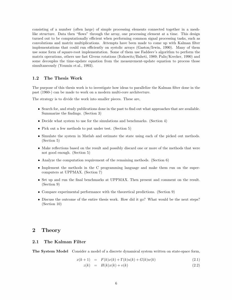
Accuracy The Fast Givens algorithm is essentially a parallel implementation of a one-step-aheadKalman predictor. Therefore it does not have the same chance of estimating the state vector asaccurately as the filtering Kalman. Table 6.5 reveals this fact.

1 2 3 4 5 6 7 8 9 10 11 12

0.5

1

1.5

2

2.5

3

x 1010

Number of cores

Flo

p pe

r fil

ter

itera

tion

Floating−point operations per filter iteration − FastGivens

n

z = 0.2n

x

nz = 0.5n

x

nz = 1.0n

x

Figure 6.4: Predicted number of floating-point operations per filter iteration, nx = 1000, nu = 2,nz = 1000, nw = 1000

33

Table 6.4: Number of floating-point operations per filter iteration for the Fast Givens algorithm

#E

xp

ress

ion

Flo

ati

ng-p

oin

top

erati

on

sp

erfi

lter

iter

ati

on

Seq

uen

tial

Para

llel

HLp

2n2 xnz−nxnz

-FLp

2n

3 x−n

2 x-

1A

=

[ I nz×nz

[HLp]

0nz×nx

0nx×nz

[FLp]

G

]2n

xnz

+n

2 z+nwnx

-

Note:

Ass

um

ing

thatA

isov

erw

ritt

en

2D

=

RDp

Q

2n

2 x+n

2 z-

3[A′ ,D′ ]

=R

ot(A,D

)39 2n

2 x+

(26nz−

39 2)nx+

1 M[5n

3 x+

(12nz−

18)n

2 x+

13 2n

2 z−

39 2nz

(9n

2 z−

27n

z+

13)nx+

2n

3 z−

9n2 z

+13nz]

4c

=z−Hx

2nxnz

-5

Sol

veLeo

=c

n3 z

-6

KzHx

=[KLe]·o

2nxnz−nx

-7

x−

=Fx

+Γu

2n

2 x+

2nunx−nx

-8

x=x−

+KzHx

nx

-9

Lp+

=A′ (nz

+1

:nz

+nx,nz

+1

:nz

+nx)

n2 x

-10

Dp+

=D′ (nz

+1

:nz

+nx,nz

+1

:nz

+nx)

n2 x

-

2n3 x

+(2nz

+49 2)n

2 x+

1 M[5n

3 x+

(12nz−

18)n

2 x+

TotalSum:

(31n

z+

2nu

+nw−

41 2)nx+

(9n

2 z−

27n

z+

13)nx+

n3 z

+17 2n

2 z−

39 2nz

2n

3 z−

9n2 z

+13nz]

34

1 2 3 4 5 6 7 8 9 10 11 121

1.5

2

2.5

3

3.5

4

Number of cores

Spe

edup

Speedup − FastGivens

n

z = 0.2n

x

nz = 0.5n

x

nz = 1.0n

x

Figure 6.5: Predicted speedup, nx = 1000, nu = 2, nz = 1000, nw = 1000

Table 6.5: Root-mean-square errors for Fast GivensFor nz = 0.2nx:

RMSnx Fast Givens Std Kalman

20 1.31 0.61500 1.22 0.711000 1.23 0.73

For nz = 0.5nx:RMS

nx Fast Givens Std Kalman

20 1.41 0.36500 1.20 0.441000 1.19 0.45

For nz = 1.0nx:RMS

nx Fast Givens Std Kalman

20 1.32 0.25500 1.25 0.261000 1.23 0.27

35

2 4 6 8 10 12

4

6

8

10

12

x 109

Number of cores

Flo

p pe

r fil

ter

itera

tion

nz = 0.2n

x

StdKalmanFusionGainFastGivens

2 4 6 8 10 12

0.6

0.8

1

1.2

1.4

1.6

x 1010

Number of cores

Flo

p pe

r fil

ter

itera

tion

nz = 0.5n

x


2 4 6 8 10 12

1

1.5

2

2.5

3

x 1010

Number of cores

Flo

p pe

r fil

ter

itera

tion

nz = 1.0n

x


Figure 6.6: Overview of the number of floating-point operations per filter iteration for different numberof outputs

6.3 Summary

Now when the analysis of the multicore performance is finished it would be interesting to do a com-parison between the methods. This can be done by setting the system order to some realistic highvalue (here nx = 1000) and plot the flops count and speedup for different number of system outputs(here nz = [ 0.2 0.5 1.0 ]nx). The results are interesting and can be seen in Figure 6.6 and 6.7.

The plots clearly show that there is no gain in using the Fusion Gain algorithm at all for small numberof outputs (the upper left plot in Figure 6.6). For a greater number of outputs the results implicate thatneither of the parallel algorithms perform better than the standard implementation of the Kalman filteron a single-core CPU. When on a dual-core or better, Fusion Gain begins to outperform the StandardKalman Filter.

Fast Givens is faster than the Standard Kalman Filter independent of the number of cores when only20 % of the states are measured. When more states are measured Fast Givens loses some of theadvantage it had over Fusion Gain, but it is still faster.

36

2 4 6 8 10 12

1

1.5

2

2.5

3

3.5

nz = 0.2n

x

Number of cores

Spe

edup

rel

ativ

e to

Std

Kal

man


2 4 6 8 10 12

1

1.5

2

2.5

3

nz = 0.5n

x

Number of cores

Spe

edup

rel

ativ

e to

Std

Kal

man


2 4 6 8 10 12

1

1.5

2

2.5

3

nz = 1.0n

x

Number of cores

Spe

edup

rel

ativ

e to

Std

Kal

man


Figure 6.7: Speedups relative to the Standard Kalman Filter

37

7 Implementation

7.1 Introduction

While the final benchmarks will be carried out on the super-computers at UPPMAX, to ease in thedevelopment process it is desirable to be able to run and debug the program on an ordinary desktopcomputer first. To achieve this, a mixture of OpenMP, BLAS, LAPACK, Intel MKL and the Cprogramming language is used.

LAPACK and BLAS To perform the matrix operations the well-known software library for numer-ical linear algebra LAPACK (Anderson et al., 1999) will be used. It contains routines for performingcommon linear algebra tasks. However, in this project, only the provided functions for performingmatrix inversion are used. The BLAS library will be used for the rest of the operations appearing inthe algorithms, e.g. matrix multiplications.

The BLAS library is specially designed to efficiently perform fundamental matrix operations such asC = αAB + βC, and is also used by LAPACK internally. The efficiency of BLAS depends heavilyon how good the BLAS library is optimized for the architecture in question. CPU vendors (e.g. Inteland AMD) provide BLAS libraries tuned to perform well on their platforms. During the developmentprocess on the desktop computer a generic, non-optimized version of BLAS was used.

BLAS and LAPACK was originally written in the programming language Fortran. Luckily there existC interfaces, like for instance CLAPACK. Unfortunately the function interface is a bit impractical touse, so I have therefore written a simple interface for each (C)LAPACK and BLAS call that I need.This greatly improves the readability of the code.

Intel MKL Intel Math Kernel Library (MKL) (Intel) is a commercial software package that includesLAPACK and BLAS libraries tuned to perform well especially on Intel’s own CPUs. The library alsotakes advantage of multiple cores when possible. Fortunately, this feature can be inactivated. This willbe needed when evaluating the different algorithms later, because we do not want MKL to interferewith our proposed parallelization strategies. However, it is not entirely necessary to inactivate thisbuilt-in feature since MKL will not parallelize anything if it detects that the program execution iswithin a OpenMP parallel section. In other words, this means that MKL calls within the sequentialparts of the algorithms will be parallelized, while calls to MKL within the parallel parts will notbe parallelized. This will still work, but to keep things simple and to be able to make theoreticalpredictions of the performance gain MKL will be set up to run single-threaded.

7.2 The Algorithms

7.2.1 Fusion-Gain

As mentioned, BLAS and LAPACK will be used to implement this algorithm. It is important to usethe non-threaded versions of these libraries, since otherwise the computations may run in parallel.Normally this would be a good thing, but in this case the purpose is to make use of the parallelizationstrategy inherited in the Fusion-Gain algorithm itself.

Table 7.1, 7.2 and 7.3 show a possible implementation of the Fusion-Gain algorithm (compare withTable 6.1), written in a way that can be directly translated into LAPACK and BLAS calls.

When a new variable (vector or matrix) is needed for storage, the dimension of that matrix is writtenin the first column. This gives a hint of the memory requirement. All variables are allocated inthe initialization part of the program, before the entrance of the simulation loop. Variables that areoverwritten during function calls are colored red.

38

Table 7.1: Implementation approach for the Global Fusion stepGlobal Fusion

For each local filter (j=1,...): This loop should be parallelized![x j, KH j, KRKT j] � Return pointers to KH j and KRKT j

Local Measurement Update(xp, P) and send the pointers to x− and P−

x(k|k) = (1−N)x(k|k − 1) +∑Nj=1 xj(k|k)

x 0 = (1-N)*xp + x 0For each local filter (j=2,...):

x 0 = x j + x 0 x 0 holds the resulting x estimationx � x 0 Pointing (no flops)

P (k|k) =[I −

∑Nj=1Kj(k)Hj(k)

]P (k|k − 1)

[I −

∑Nj=1Kj(k)Hj(k)

]T+∑Nj=1Kj(k)Rj(k)KT

j (k)

KH 0 = I - KH 0 z is overwrittenFor each local filter (j=2,...):

KH 0 = KH 0 - KH j KH 0 holds the sum KH j

For each local filter (j=2,...):KRKT 0 = KRKT j + KRKT 0 KRKT 0 holds the sum KRKT j

nx × nx t1Pp = KH 0*PpKRKT 0 = t1Pp*KH 0’ + KRKT 0P � KRKT 0 Pointing (no flops)

Table 7.2: Implementation approach for the Local Measurement-Update stepLocal Measurement-Update

nx x j = x Make a copy of the global x vector

Kj(k) = 1γP (k|k − 1)HT

j (k)(Hj(k)P (k|k − 1)HT

j (k) + 1γRj(k)

)−1

nz × nx HP j = H j*Pnz × nz HPHT R j = lti.R Make a copy to avoid losing the data

HPHT R j = HP j * lti.H’ + 1γHPHT R j Where HPHT R was lti.R originally

HPHT R j = inv(HPHT R j)nx × nz PHT j = 1

γP*lti.H’

nx × nz K j = PHT j * HPHT R j

xj(k|k) = xj(k|k − 1) +Kj(k) (zj(k)−Hj(k)xj(k|k − 1))nz z j = -lti.H*xp + z j Parts of the original z vector is overwritten

x j = K j*z + x j

Kj(k)Hj(k)nx × nx KH j = K j*lti.H

Kj(k)Rj(k)KTj (k)

nx × nz KR j = K j*Rnx × nx KRKT j = KR j * K’ j

39

Table 7.3: Implementation approach for the Global Time-Update stepGlobal Time-Update

x(k + 1|k) = F (k)x(k|k) + Γ(k)u(k)nx xp = lti.F*x Has to be separate x vectors to work with the function

xp = lti.Γ*u + xp

P (k + 1|k) = F (k)P (k)FT (k) +G(k)Q(k)GT (k)nx × nw GQ = lti.G*lti.Qnx × nx Pp = GQ*lti.G’nx × nx FP = lti.F*P

Pp = FP*lti.F’ + Pp

From Table 7.1 it is clear that this is the section that should be parallelized. For this the OpenMPstatement “parallel for” can be used. The following code snippet shows how this may look like,

#pragma omp p a r a l l e l shared ( z a r r , xp , Pp , l t i l o c a l s , w r l o c a l s ) p r i v a t e ( i ){#pragma omp f o r

f o r ( i =0; i<n l o c a l s ; i++) {fus ionGainLocalExec ( z a r r [ i ] , xp , Pp , &l t i l o c a l s [ i ] , &w r l o c a l s [ i ] ) ;

}}

The “shared” and “private” clauses specify the scopes of the variables. As can be seen most of thevariables (pointers in this case) are shared among the threads. This is perfectly valid since the pointersdo not change their values. The iteration variable, i however, does change and should therefore not bedeclared as “shared”. Declaring i “private” ensures that each thread has its own copy of it.

7.2.2 Fast Givens Rotation

The Fast Givens method (Algorithm 11 and 12) together with the modifications proposed in Section6.2 are used as the basis for the implementation. BLAS and LAPACK will be used for the matrixoperations before and after the rotation. The rotation itself (Algorithm 12) does not use ordinarymatrix operations at all, and is more about looping through the matrix and performing simple scalaroperations on the matrix elements.

7.3 The Benchmark Software

The benchmark program will behave very similar to the MATLAB program used earlier in the analysisof the algorithms. A key difference is that this program will take advantage of multiple cores throughthe use of OpenMP. Also, a timer has been included that measures the speed of the algorithms fordifferent simulation setups. A simulation setup is defined by e.g. the system model, the number ofcores, initial values of the state vector (x0) and the initial value of the state error covariance matrix(P0).

The problem with a low-level language like C is that it easier to make mistakes during coding. Toreduce the possibility of errors, all output from the program is written to data log files containing thecomputed state estimations together with the current simulation setup. It is then possible to comparethis with the data output from the original MATLAB script. This approach has been taken to verifythe correctness of the C implementation.

40

8 Preparations for the Final Run

8.1 Setting up the Test Cases

Main Test It is now time to stage the final test of the proposed algorithms. The most interestingpart is perhaps to determine the speedup factor for different benchmark setups. The plan is to dothis for a small system model consisting of 20 states, a medium sized model of order 500 and a largemodel of order 1000. The expected outcome of this test is to see that there will be little or no gain inapplying the parallel algorithms to a small model, due to the overhead involved in the OpenMP fork-join process. As the model order increases the signs of the overhead will decay, and both of the parallelalgorithms will hopefully perform better than the standard sequential Kalman filter. According to theoutcome of the algorithm analysis in Section 6, the speedup will increase even further as the modelorder grows larger.

To see how the speedup is also affected by the number of system outputs, nz will vary as 20 %, 50 %and 100 % of the model order nx.

For the “Fusion Gain” algorithm, different number of local subsystems will be tested to see how itaffects the performance.

Since the computations will be performed on quad-core CPUs, the number of threads to test thealgorithms on will be 1, 2, 3 and 4 respectively.

Cache Size Limit Additional tests will be carried out to investigate when the limited cache sizebecomes a bottle neck. For small problem sizes the Flops (“Floating-point operations per second”)capability of the CPU is assumed to be the limiting factor. But for large systems there will not beenough space in the cache to hold the same amount of data. To see when this happens, the idea is tonotice when the experimental measurements start to divagate from the theoretical predictions, or inother words, when the time measure does no longer increase as O(n3

x).

A Word on the Fusion Gain Algorithm The Fusion Gain algorithm has an extra variable thataffects the performance noticeable, namely the number of subsystems to divide the full system in. Tomake things simple, the “natural” choice, of having the same number of subsystems as the number ofcores has been selected. This means that when the speedup plot of the Fusion Gain algorithm itself isgenerated, the speedup values will be relative to the time it would take to run the algorithm with thesame number of subsystems on a single-core CPU. This choice prevents the speedup plot from possiblygive false hopes of greater than linear speedup, which otherwise would be possible as mentioned in theanalysis of the algorithm (Section 6.1).

When comparing to the standard sequential Kalman algorithm the speedups will be relative to preciselythe same standard sequential Kalman filter at all points in the plot.

8.2 Computer Environment

To get accurate time measures on how the algorithms perform, it is desirable to use a multi-corecomputer system with as few other running processes as possible. The computers at Uppsala Mul-tidisciplinary Center for Advanced Computational Science (UPPMAX) fulfill this criteria perfectly.UPPMAX has three different multicore systems (Kalkyl, Grad and Halvan). The benchmarks will becarried out on Kalkyl, which is a cluster of 348 computer nodes, where each node has two Intel 5520quad-core CPUs, each on with 8 MB of shared memory among the four cores. Because this work isfocused towards the multicore architecture, only one quad-core CPU on one node will be used.

To run “jobs” at UPPMAX it is neccessay to use a batch system called SLURM. Jobs can either berun in the background (“batch mode”) or in the foreground (“interactive mode”). Interactive jobs are

41

1 2 3 40

0.5

1

1.5

2


x

Tim

e [s

]

Number of cores

n

x = 20

nx = 500

nx = 1000

1 2 3 40

0.5

1

1.5

2

2.5


x

Tim

e [s

]

Number of cores

n

x = 20

nx = 500

nx = 1000

1 2 3 40

1

2

3

4


x

Tim

e [s

]

Number of cores

n

x = 20

nx = 500

nx = 1000

Figure 9.1: Fusion Gain, experimental measurement

limited to run for at most one hour and typically starts right away. To run longer jobs or run morethan one job simultaneously batch jobs have to be used. These are slightly more complicated to setup, so for this work everything have been run in interactive mode using the command,

i n t e r a c t i v e −A p2008031 −−e x c l u s i v e −N 1 −n 8 −t 1 : 0 0 : 0 0

This starts an interactive session on one compute node (“-N1”). “–exclusive -n8” guarantees sole accessto an entire compute node.

All BLAS and LAPACK functionality has been provided by the Intel MKL library.

9 Final Results

9.1 Fusion Gain

The first results from the benchmark run are shown in Figure 9.1. All time measurements are decayingwhich is promising. For later comparison to the theoretical predictions Figure 9.2 is more informative.It tells that this method benefits from being run on a multi-core system which is in line with thepredictions.

Comparison with Sequential Kalman The grand test is to see how the algorithms compare to theStandard Kalman Filter. Figure 9.3 shows that there is no use in choosing the Fusion Gain algorithmwhen the number of measured signals is small, since it is then slower than the Standard Kalman filter.At nz = 0.5nx, Fusion Gain becomes almost equal to the Standard Kalman filter performance wise.When all states are measured one can expect a speedup of about 1.5. The algorithm generally performsworse for small systems (order 20 in these cases) because of the overhead as mentioned earlier in thereport.

42

1 2 3 41

1.1

1.2

1.3

1.4


x

Number of cores

Spe

edup

n

x = 20

nx = 500

nx = 1000

1 2 3 41

1.1

1.2

1.3

1.4

1.5


x

Number of cores

Spe

edup

n

x = 20

nx = 500

nx = 1000

1 2 3 41

1.2

1.4

1.6

1.8


x

Number of cores

Spe

edup

n

x = 20

nx = 500

nx = 1000


1 2 3 40.8

0.82

0.84

0.86

0.88

0.9


x

Speedup relative to StdKalman

Number of cores

Spe

edup

n

x = 20

nx = 500

nx = 1000

1 2 3 40.7

0.8

0.9

1

1.1


x


Number of cores

Spe

edup

n

x = 20

nx = 500

nx = 1000

1 2 3 4

0.8

1

1.2

1.4

1.6


x


Number of cores

Spe

edup

n

x = 20

nx = 500

nx = 1000


43

1 2 3 40

5

10

15

FastGivens, nz = 0.2n

x

Tim

e [s

]

Number of cores

n

x = 20

nx = 500

nx = 1000

1 2 3 40

5

10

15

20

25


x

Tim

e [s

]

Number of cores

n

x = 20

nx = 500

nx = 1000

1 2 3 40

10

20

30

40


x

Tim

e [s

]

Number of cores

n

x = 20

nx = 500

nx = 1000

Figure 9.4: Fast Givens, experimental measurement

9.2 Fast Givens

The time consumed by the Fast Givens algorithm is presented in Figure 9.4 and the self-speedup inFigure 9.5.

The experimental results make clear that it is meaningless to apply this implementation of the FastGivens algorithm on small systems. The speedups for nx = 20 are not just less than 1, but also getworse when increasing the number of cores.

For the larger systems (nx = 500 and nx = 1000) the speedup increases with the number of cores.

Comparison with Sequential Kalman Figure 9.6 illustrates how much faster Fast Givens is inrelation to the Standard Kalman filter. Unfortunately, it shows that the Fast Givens approach is notnearly as fast as a Standard Kalman Filter in neither of the situations. The only thing that couldpossibly favor the Fast Givens algorithm is its better numerical stability.

9.3 Experimental versus Predicted Results

Fusion Gain With the benchmark results in hand, it is possible to evaluate how well the predictedspeedups compare to the real ones. Figure 9.7 shows the self speedup of the Fusion Gain algorithmfor nz = 0.5nx. The dashed lines are the predicted speedups as derived in Section 6.1.

It can be concluded that the theoretical predictions align almost perfectly with the measured speedupsfor nx = 500 and nx = 1000.

The small system (nx = 20) actually performs significantly better than the predicted, which could becache size related. The speedup numbers are computed as the time it takes to run the algorithm onjust one core divided by the time it takes to run the same algorithm on more than one core. Becauseof the structure of the Fusion Gain algorithm the amount of data handled by each core decreases as

44

1 2 3 40

0.5

1

1.5

2


x

Number of cores

Spe

edup

n

x = 20

nx = 500

nx = 1000

1 2 3 40

0.5

1

1.5

2

2.5


x

Number of cores

Spe

edup

n

x = 20

nx = 500

nx = 1000

1 2 3 40

0.5

1

1.5

2

2.5


x

Number of cores

Spe

edup

n

x = 20

nx = 500

nx = 1000


1 2 3 40

0.05

0.1

0.15

0.2

0.25


x


Number of cores

Spe

edup

n

x = 20

nx = 500

nx = 1000

1 2 3 40

0.05

0.1

0.15

0.2


x


Number of cores

Spe

edup

n

x = 20

nx = 500

nx = 1000

1 2 3 40

0.05

0.1

0.15

0.2


x


Number of cores

Spe

edup

n

x = 20

nx = 500

nx = 1000


45

1 2 3 41

1.05

1.1

1.15

1.2

1.25

1.3

1.35

1.4

1.45FusionGain

nx=20 (predicted)nx=20 (measured)nx=500 (predicted)nx=500 (measured)nx=1000 (predicted)nx=1000 (measured)

Figure 9.7: Fusion Gain, Theory vs. Practice (nz = 0.5nx)

the number of cores increases. So a significant amount of cache misses are likely to occur in the singlecore case, which causes the speedups to grow.

Fast Givens The speedup plot for the Fast Givens method does not correspond as well with thetheoretical prediction as in the Fusion Gain case (Figure 9.8). The experimental speedup numbers aresomewhat smaller than the predicted ones.

The nx = 1000 system lies closer to the theoretical value than the smaller system nx = 500, and thenx = 20 system especially. The reason for this could either be a bad theoretical analysis or, morelikely, extra computation costs involved in the parallelization of the actual Fast Givens rotation, sinceit is the only part that is parallelized in the algorithm. More precisely, the overhead from the fork-joinprocedure could probably be blamed for this. As mentioned earlier in the report, the parallelizablework decreases for each iteration in the loop which leads to an increase in overhead.

Comparison to the Standard Kalman Filter If the speedup plots (Figure 9.3 and 9.6, fornx = 1000) are compared to the predicted speedups in relation to the standard Kalman filter presentedin Figure 6.7, it can be seen that the speedup curves for the Fusion Gain match up fairly well. TheFast Givens method on the other hand, is much slower in reality, e.g. 2.2 in theory and less than 0.2 inpractice (4 cores, nx = 1000, nz = 0.5nx). This suggests that the theoretical analysis of the number offloating-point operations per filter iteration is not perfect when it comes to modeling absolute executiontime.

46

1 2 3 40

0.5

1

1.5

2

2.5

3FastGivens

nx=20 (predicted)nx=20 (measured)nx=500 (predicted)nx=500 (measured)nx=1000 (predicted)nx=1000 (measured)

Figure 9.8: Fast Givens, Theory vs. Practice (nz = 0.5nx)

47

9.4 Intel MKL with Thread Support Enabled

Up to this point, only benchmark runs that could be supported by the theoretical analysis done inSection 6 have been considered. In real life situations however, where a fast estimator is needed, onewould probably do even without such an analysis as long as it performs well. Previously in the report,it was mentioned that all benchmarks would be run with thread support disabled in the Intel MKLlibrary. In this section benchmark results are presented with thread support enabled. This means thatMKL routines such as matrix multiplication and inversion make use of parallelism internally.

The first result shows the self-speedup of the standard Kalman filter algorithm (Figure 9.9). It canbe noticed that the speedup increases almost linearly with the number of cores when few states areobserved. Then, as more states are observed the speedup drops, e.g. to 3 when 4 cores are used (fornz = nx). Still it performs much better compared to what was seen in earlier plots.

1 2 3 41

2

3

4

StdKalman, nz = 0.2n

x

Number of cores

Spe

edup

n

x = 20

nx = 500

nx = 1000

1 2 3 41

2

3

4


x

Number of cores

Spe

edup

n

x = 20

nx = 500

nx = 1000

1 2 3 41

2

3

4


x

Number of cores

Spe

edup

n

x = 20

nx = 500

nx = 1000

Figure 9.9: Self-speedup for Standard Kalman Filter algorithm (threaded MKL)

When MKL thread support is enabled and the execution reaches an OpenMP parallel section, none ofthe MKL calls therein will make use of threading. In the case with the Fusion Gain method, this meansthat MKL calls in the local measurement-update step (Table 7.2) do not take advantage of multiplecores. All cores are still utilized however, since each core runs its own local measurement-update step.During the two other steps (Global Time-Update and Global Fusion) MKL routines are threaded sincethey take place outside the parallel section.

When just considering the self-speedup plot (Figure 9.10) all three curves lie somewhere between thenz = 0.2nx and nz = 1.0nx curves of the standard Kalman filter (Figure 9.9).

48

1 2 3 41

2

3

4


x

Number of cores

Spe

edup

n

x = 20

nx = 500

nx = 1000

1 2 3 41

2

3

4


x

Number of cores

Spe

edup

n

x = 20

nx = 500

nx = 1000

1 2 3 41

2

3

4


x

Number of cores

Spe

edup

n

x = 20

nx = 500

nx = 1000

Figure 9.10: Self-speedup for Standard Kalman Filter algorithm (threaded MKL)

It is not possible to tell which method is the faster by just looking at the self-speedup plots. Figure9.11 shows how much faster the Fusion Gain algorithm is compared to the standard Kalman filter (withthreading enabled). This plot reveals that the standard Kalman filter is faster even for nz = 0.5nx (asopposite to the previous conclusion made from Figure 9.3). The standard Kalman filter apparentlyhas more to win on enabling the threaded MKL library, but the Fusion Gain method is still faster inthe many-outputs case.

49

1 2 3 40.7

0.75

0.8

0.85

0.9

0.95


x


Number of cores

Spe

edup

n

x = 20

nx = 500

nx = 1000

1 2 3 40.7

0.8

0.9

1

1.1


x


Number of cores

Spe

edup

n

x = 20

nx = 500

nx = 1000

1 2 3 4

0.8

1

1.2

1.4


x


Number of cores

Spe

edup

n

x = 20

nx = 500

nx = 1000

Figure 9.11: Speedup for the Fusion Gain algorithm relative to the Standard Kalman Filter (threadedMKL)

10 Discussion

10.1 Conclusions

The results from the benchmark indicate that in some situations it could be advantageous to use theFusion Gain algorithm instead of the Kalman filter implemented on standard form. These situationsare when a large portion of the state variables are measured. When measured on a quad-core computerthe speedup turned out to be about 1.5 for the tested systems of order 500 and 1000. For the system oforder 20, the speedup was around 1.2. The lower speedup could be explained by increasing overheadtime in relation to the total execution time.

If 50 % or fewer of the state variables were measured, there was no point in trading the standardKalman filter for the Fusion Gain filter. Actually, because of the slightly worse numerical accuracywith Fusion Gain, the standard Kalman filter is definitely preferable.

The Kalman filter using the Fast Givens algorithm was a let-down. It did not perform nearly as goodas it was supposed to according to the predictions. In all tested cases it was much slower than thestandard Kalman filter. Its state estimates also got further away from the true states than both theFusion Gain algorithm and the standard Kalman filter. This is natural because the algorithm in theoriginal paper was constructed as a one-step-ahead predictor, i.e. it uses measurements from time k toestimate the state vector at k+ 1. However, the method should be more numerically stable comparedto both the other filters, because it is based on a square-root algorithm.

50

Theoretical Predictions The number of floating-point operations per filter iteration predictionsderived in Section 6 were quite accurate when it came to predict the self-speedups for both algorithms,but were not perfect.

When comparing with the standard Kalman filter, the Fast Givens method performed significantlyworse than predicted. This suggests that the theoretical Flops analysis has issues when it comesto modeling absolute execution time. In this particular algorithm implementation the number ofpure floating point operations is quite small compared to the rest of the machine code, e.g. loopingoverhead and bad instruction pipeline usage. The Fusion Gain algorithm and the standard Kalmanfilter algorithm are more similar to each other in that they both spend most if the computation timein matrix algebra library routines (Intel MKL in this case).

The predictions were made solely on the number of Flops which explains why it could not perfectlypredict the speedup in some cases. As mentioned in Section 9 other factors also have impact on thethe actual speedup, for instance limited memory bandwidth, cache sizes and overhead. If those factorswere modeled as well, the predictions would probably have been even more accurate.

Altough not perfect, the theoretical analysis still serves the purpose of predicting how well the algo-rithms will work in reality. Without any type of theoretical analysis it would be difficult to know whatto expect from the implemented algorithms.

As a side-note, the expression-to-Flops generator, mentioned earlier in the report, proved to be veryuseful in reducing the risk of human errors, when computing the Flops for each expression in the twoalgorithms (Fusion Gain and Fast Givens).

Threaded MKL At the end of the previous section, benchmarks were run to determine how thebuilt-in threading in the Intel MKL library would affect the results. The results showed that thestandard implementation of the original Kalman filter, without any modifications, benefited greatlyfrom multiple cores. The Fusion Gain algorithm also took advantage of the threading used in the MKLcalls in the sequential sections of the algorithm. In the parallel section (Local Measurement-Update)threading within the MKL routines was disabled automatically.

The conclusion drawn from these tests is that the Fusion Gain algorithm is only to prefer (performancewise) over a standard implementation of the Kalman filter when having a very large output vector.

10.2 Future Work

Unsolved issues were discovered when simulating (Section 5.2) the distributed Kalman filter describedin Section 3.1.1. It is unclear where the error source lies. This lead to that method, and the reduced-order method too, being discarded from this survey. If the problem could be solved, there might be achance for these algorithms to become useful.

It is also doubtful whether this method is any faster than the one originally described in (Willner/Chang/Dunn, 1976). The authors of (Hashemipour/Roy/Laub, 1988) claim that their method is moreefficient because it does not need to communicate the global estimate back to the local filters, but ina multi-core environment the cost might not be too big to still be of use. Besides, making sure thateach local filter gets hold of the global estimate should lead to improved robustness of the algorithm.So, this method might also be worth to take a further look at.

To avoid numerical instability in real life applications some sort of square-root implementation ispreferable. For the Fusion Gain algorithm to be useful in such cases, it should somehow be convertedinto square-root form.

The Fast Givens method deserves more attention. The theoretical prediction tells that this methodconsumes fewer number of floating-point operations per filter iteration than both the other methods.Still, it performs very bad according to the benchmarks.

It would be interesting to see if the theoretical computation time analysis could be improved, i.e. notonly depend on the pure Flops usage.

51

References

Anderson, E. et al.: LAPACK Users’ Guide. 3rd edition. Philadelphia, PA: Society for Industrialand Applied Mathematics, 1999, ISBN 0–89871–447–8 (paperback)

Carlson, N.A.: Federated square root filter for decentralized parallel processors. Aerospace andElectronic Systems, IEEE Transactions on, 26 may 1990 No. 3, 517 –525, ISSN 0018–9251

Chong, C. Y.: Hierarchical estimation. Proc. 2nd MIT/ONR C3 Workshop july 1979

Faxen, Karl-Filip et al.: Multicore computing - the state of the art. 2008

Gaston, F.M.F./Irwin, G.W.: Systolic Kalman filtering: an overview. Control Theory and Appli-cations, IEE Proceedings D, 137 jul 1990 No. 4, 235 – 244, ISSN 0143–7054

Gustafsson, Fredrik: Adaptive Filtering and Change Detection. Wiley, October 2000 〈URL: http://www.wiley.com/WileyCDA/WileyTitle/productCd-0471492876,descCd-description.

html〉, 510, ISBN ISBN: 978–0–470–85340–5

Hashemipour, H.R./Roy, S./Laub, A.J.: Decentralized structures for parallel Kalman filtering.Automatic Control, IEEE Transactions on, 33 jan 1988 No. 1, 88 –94, ISSN 0018–9286

Heath, M. T.: Scientific computing: an introductory survey. 2002

Hoffmann, H./Devadas, S./Agarwal, A.: A Pattern for Efficient Parallel Computation on Mul-ticore Processors with Scalar Operand Networks. 2010

Intel: Math Kernel Library. http://developer.intel.com/software/products/mkl/

Itzkowitz, Howard R./Baheti, Radhakisan S.: Demonstration of Square Root Kalman Filter onWarp Parallel Computer. In American Control Conference, 1989. june 1989, 1754 –1762

Kalman, Rudolph Emil: A New Approach to Linear Filtering and Prediction Problems. Transac-tions of the ASME–Journal of Basic Engineering, 82 1960 No. Series D, 35–45

Kung, H.T.: The Warp Processor: A Versatile Systolic Array for Very High Speed Signal Processing.1984

Kung, H.T./Leiserson, C.E./Computer Science, Carnegie-Mellon University. Dept. of:Systolic Arrays for (VLSI). Carnegie-Mellon University, Department of Computer Science, 1978,CMU-CS 〈URL: http://books.google.se/books?id=pAKfHAAACAAJ〉

Mcgee, L.A.: Discovery of the Kalman filter as a practical tool for aerospace and industry. 1985〈URL: http://books.google.se/books?id=PXVGAQAAIAAJ〉

Paik, B.S./Oh, J.H.: Gain fusion algorithm for decentralised parallel Kalman filters. Control Theoryand Applications, IEE Proceedings -, 147 jan 2000 No. 1, 97 –103, ISSN 1350–2379

Palis, M.A./Krecker, D.K.: Parallel Kalman filtering on the Connection Machine. In Frontiers ofMassively Parallel Computation, 1990. Proceedings., 3rd Symposium on the. October 1990, 55–58

Roy, S./Hashemi, R.H./Laub, A.J.: Square root parallel Kalman filtering using reduced-orderlocal filters. Aerospace and Electronic Systems, IEEE Transactions on, 27 mar 1991 No. 2, 276–289, ISSN 0018–9251

Vinjamuri, Sudhir/Prasanna, Viktor: Hierarchical Dependency Graphs: Abstraction andMethodology for Mapping Systolic Array Designs to Multicore Processors. In Proceedings of the10th International Conference on Parallel Computing Technologies. Berlin, Heidelberg: Springer-Verlag, 2009, PaCT ’09 〈URL: http://dx.doi.org/10.1007/978-3-642-03275-2_28〉, ISBN978–3–642–03274–5, 284–298

52

http://www.wiley.com/WileyCDA/WileyTitle/productCd-0471492876,descCd-description.html



http://developer.intel.com/software/products/mkl/

http://books.google.se/books?id=pAKfHAAACAAJ

http://books.google.se/books?id=PXVGAQAAIAAJ

http://dx.doi.org/10.1007/978-3-642-03275-2_28

Willner, D./Chang, C. B./Dunn, K. P.: Kalman filter algorithms for a multi-sensor system. InDecision and Control including the 15th Symposium on Adaptive Processes, 1976 IEEE Confer-ence on. Volume 15, 1976, 570 –574

Youmin, Zhang et al.: A parallel decoupled Kalman filtering algorithm and systolic architecture. InDecision and Control, 1993., Proceedings of the 32nd IEEE Conference on. dec 1993, 3590 –3595vol.4

53

Documents

Parallelization of the Kalman filter for multi-output systems on