Embed Size (px)
Citation preview
HELSINKI UNIVERSITY OF TECHNOLOGY Department of Electrical and Communications Engineering Olli Mäkelä
PARAMETER ESTIMATION FOR A SYNCHRONOUS MACHINE Master’s thesis submitted in partial fulfillment of the requirements for the degree of Master of Science in Technology
Espoo 17.8.2007
Supervisor
Professor Antero Arkkio
Instructor
M.Sc. Anna-Kaisa Repo
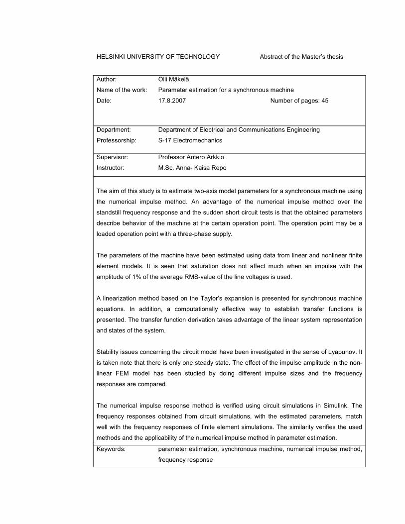
HELSINKI UNIVERSITY OF TECHNOLOGY Abstract of the Master’s thesis
Author: Olli Mäkelä
Name of the work: Parameter estimation for a synchronous machine
Date: 17.8.2007 Number of pages: 45
Department: Department of Electrical and Communications Engineering
Professorship: S-17 Electromechanics
Supervisor: Professor Antero Arkkio
Instructor: M.Sc. Anna- Kaisa Repo
The aim of this study is to estimate two-axis model parameters for a synchronous machine using
the numerical impulse method. An advantage of the numerical impulse method over the
standstill frequency response and the sudden short circuit tests is that the obtained parameters
describe behavior of the machine at the certain operation point. The operation point may be a
loaded operation point with a three-phase supply.
The parameters of the machine have been estimated using data from linear and nonlinear finite
element models. It is seen that saturation does not affect much when an impulse with the
amplitude of 1% of the average RMS-value of the line voltages is used.
A linearization method based on the Taylor’s expansion is presented for synchronous machine
equations. In addition, a computationally effective way to establish transfer functions is
presented. The transfer function derivation takes advantage of the linear system representation
and states of the system.
Stability issues concerning the circuit model have been investigated in the sense of Lyapunov. It
is taken note that there is only one steady state. The effect of the impulse amplitude in the non-
linear FEM model has been studied by doing different impulse sizes and the frequency
responses are compared.
The numerical impulse response method is verified using circuit simulations in Simulink. The
frequency responses obtained from circuit simulations, with the estimated parameters, match
well with the frequency responses of finite element simulations. The similarity verifies the used
methods and the applicability of the numerical impulse method in parameter estimation.
Keywords: parameter estimation, synchronous machine, numerical impulse method,
frequency response
TEKNILLINEN KORKEAKOULU Diplomityön tiivistelmä
Tekijä: Olli Mäkelä
Työn nimi: Tahtikoneen parametrien estimointi
Päivämäärä: 17.8.2007 Sivumäärä: 45
Osasto: Sähkö- ja tietoliikennetekniikan osasto
Professuuri: S-17 Sähkömekaniikka
Työn valvoja: Professori Antero Arkkio
Työn ohjaaja: DI Anna- Kaisa Repo
Tämän työn tavoitteena on estimoida tahtikoneen kaksiakselimallin parametrit käyttäen
numeerista impulssimenetelmää. Esitetyn menetelmän etu on, että saadut parametrit kuvaavat
todellista toimintapistettä, toisin kuin harmonisen taajuusanalyysin ja oikosulkukokeen avulla
saadut parametrit.
Tahtikoneen parametrit on arvioitu käyttäen lineaarista ja epälineaarista elementtimenetelmä-
mallia. Huomataan, että kyllästyminen ei juuri vaikuta taajuusvasteisiin, kun käytetään 1 %
verkkojännitteen RMS-arvon suuruista impulssia.
Työssä esitetään Taylorin kehitelmään perustuva lineaarisointimenetelmä tahtikoneen yhtälöille.
Lisäksi esitetään laskennallisesti tehokas menetelmä siirtofunktion muodostamiseen, jossa
käytetään lineaarisen systeemin esitystä ja tiloja hyväksi.
Piirimallille on suoritettu stabiilisuustarkastelu Lyapunovin mielessä. Todetaan, että systeemillä
on vain yksi pysyvä tila. Syötetyn impulssin amplitudin suuruuden vaikutusta taajuusvasteeseen
elementtimenetelmän epälineaarisessa mallissa tutkitaan käyttämällä erisuuruisia impulsseja.
Numeerisen impulssimenetelmän toimivuus on osoitettu todeksi piirimallilla tehtyjen
simulaatioiden avulla Simulink- ympäristössä. Piirimallissa on käytetty estimoituja parametreja.
Piirimallilla tehtyjen simulaatioiden taajuusvasteet vastasivat hyvin FEM simulaatioilla saatuja
taajuusvasteita. Taajuusvasteiden yhteneväisyys osoittaa todeksi käytetyt menetelmät ja
numeerisen impulssimenetelmän käyttökelpoisuuden parametrien estimoinnissa.
Avainsanat: parametrien estimointi, tahtikone, numeerinen impulssimenetelmä, taajuusvaste

Foreword This work has been carried out in the Laboratory of Electromechanics at Helsinki
University of Technology, TKK, during the spring and summer 2007. I would like to thank
my instructor Anna-Kaisa Repo and supervisor Antero Arkkio for advices, comments and
help during this study.
I would also like to thank Jarmo Perho, Marko Hinkkanen and Mikaela Cederholm for
instructive discussions we had during my project. Additionally, I thank Jan Westerlund
from ABB Oy for providing data of the studied machine.
Finally, I would like to thank my parents, siblings and friends for support during my
studies.
In Otaniemi, August 2007
Olli Mäkelä
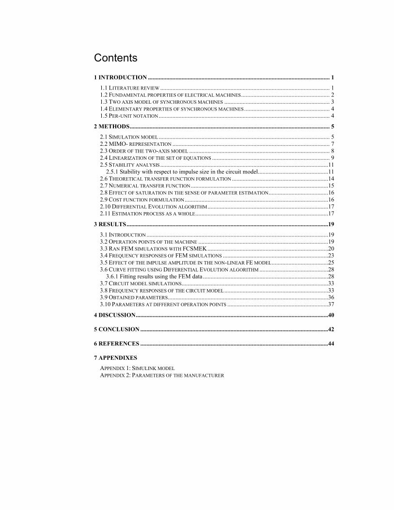
Contents
1 INTRODUCTION ....................................................................................................................... 1
1.1 LITERATURE REVIEW ............................................................................................................... 1 1.2 FUNDAMENTAL PROPERTIES OF ELECTRICAL MACHINES.......................................................... 2 1.3 TWO AXIS MODEL OF SYNCHRONOUS MACHINES ..................................................................... 3 1.4 ELEMENTARY PROPERTIES OF SYNCHRONOUS MACHINES ........................................................ 4 1.5 PER-UNIT NOTATION ................................................................................................................ 4
2 METHODS................................................................................................................................... 5
2.1 SIMULATION MODEL ................................................................................................................ 5 2.2 MIMO- REPRESENTATION ....................................................................................................... 7 2.3 ORDER OF THE TWO-AXIS MODEL ............................................................................................ 8 2.4 LINEARIZATION OF THE SET OF EQUATIONS ............................................................................. 9 2.5 STABILITY ANALYSIS ..............................................................................................................11 2.5.1 Stability with respect to impulse size in the circuit model..............................................11
2.6 THEORETICAL TRANSFER FUNCTION FORMULATION ...............................................................14 2.7 NUMERICAL TRANSFER FUNCTION ..........................................................................................15 2.8 EFFECT OF SATURATION IN THE SENSE OF PARAMETER ESTIMATION.......................................16 2.9 COST FUNCTION FORMULATION..............................................................................................16 2.10 DIFFERENTIAL EVOLUTION ALGORITHM ...............................................................................17 2.11 ESTIMATION PROCESS AS A WHOLE.......................................................................................17
3 RESULTS....................................................................................................................................19
3.1 INTRODUCTION .......................................................................................................................19 3.2 OPERATION POINTS OF THE MACHINE .....................................................................................19 3.3 RAN FEM SIMULATIONS WITH FCSMEK...............................................................................20 3.4 FREQUENCY RESPONSES OF FEM SIMULATIONS .....................................................................23 3.5 EFFECT OF THE IMPULSE AMPLITUDE IN THE NON-LINEAR FE MODEL.....................................25 3.6 CURVE FITTING USING DIFFERENTIAL EVOLUTION ALGORITHM .............................................28 3.6.1 Fitting results using the FEM data ..................................................................................28
3.7 CIRCUIT MODEL SIMULATIONS................................................................................................33 3.8 FREQUENCY RESPONSES OF THE CIRCUIT MODEL ....................................................................33 3.9 OBTAINED PARAMETERS.........................................................................................................36 3.10 PARAMETERS AT DIFFERENT OPERATION POINTS ..................................................................37
4 DISCUSSION..............................................................................................................................40
5 CONCLUSION ...........................................................................................................................42
6 REFERENCES ...........................................................................................................................44
7 APPENDIXES
APPENDIX 1: SIMULINK MODEL APPENDIX 2: PARAMETERS OF THE MANUFACTURER

Symbols and acronyms
Symbols
e error
f frequency
G transfer function
i current
I inertia
j complex variable
J rotation matrix
L inductance of an inductor
p number of pole pairs
P power
R resistance of a resistor
s Laplace operator
t time
T torque
u voltage
Y admittance
Z impedance
Greek symbols
∆ deviation
ψ flux
ω angular frequency
Ω mechanical speed
Subscripts
0 operation point
B base value
d direct axis
D direct axis damper winding
e electrical
f field winding
imp impulse
m mechanical

mr mutual component in rotor
ms mutual component in stator
q quadrature axis
Q quadrature axis damper winding
r rotor
rel relative amplitude
rms root mean square
s stator
Acronyms
DE Differential Evolution
FE finite element
FEA finite element analysis
FEM finite element method
MIMO multiple input multiple output
p. u. per unit
SSFR stand still frequency response
1
1 Introduction
This master’s thesis deals with parameter estimation for a synchronous machine. A
conventional two-axis circuit model is adequate for many applications, provided the
parameters are properly defined. The aim of this study is to introduce new sights in
parameter estimation against previous and conventional methods.
The appropriate parameter values are essential in control design and in power system
applications. With accurate parameter values, the behavior of a machine can be
predicted well.
Nowadays, finite element analysis (FEA), Bastos, J. P. A. et al. (2003), is the state of the
art in electrical machine design. The FEA gives accurate results, and in that perspective,
it is natural that parameter estimation process using FEA would be a good approach in
order to get competent parameter values.
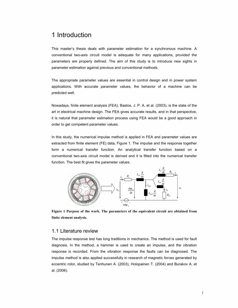
In this study, the numerical impulse method is applied in FEA and parameter values are
extracted from finite element (FE) data, Figure 1. The impulse and the response together
form a numerical transfer function. An analytical transfer function based on a
conventional two-axis circuit model is derived and it is fitted into the numerical transfer
function. The best fit gives the parameter values.
du
qωψ-+
sR
DR
fR
sd
d
dL
t
f
d
dL
t
D
d
dL
t
md
d
dL
t
fu
di
Di
fi
dd
dt
ψ
mdi
Figure 1 Purpose of the work. The parameters of the equivalent circuit are obtained from
finite element analysis.
1.1 Literature review
The impulse response test has long traditions in mechanics. The method is used for fault
diagnosis. In the method, a hammer is used to create an impulse, and the vibration
response is recorded. From the vibration response the faults can be diagnosed. The
impulse method is also applied successfully in research of magnetic forces generated by
eccentric rotor, studied by Tenhunen A. (2003), Holopainen T. (2004) and Burakov A. et
al. (2006).
2
An idea of using the numerical impulse method in FEA to estimate the parameters of an
equivalent circuit is not widely studied. However, Repo A.-K. et al. (2006a, 2006b & 2007)
have studied these issues for induction machines in three papers. The idea behind the
impulse response test is to apply an excitation, which includes many frequencies. Thus
we can avoid the usage of the harmonic excitation that means supplying one excitation
frequency at a time.
There are no publications studying this method for synchronous machines. Therefore the
aim of this study is also to check the applicability of this method for synchronous
machines.
The Institute of Electrical and Electronics Engineers (IEEE) (1995) presents guidelines for
parameter estimation for a synchronous machine. There are also publications written, for
example, by Keyhani, A. et al. (1994) and Bortoni, E. C. et al. (2004), about parameter
estimation for synchronous machines using standstill frequency response (SSFR). In the
SSFR, it is assumed that the resistance of windings is determined by other means and
the machine is tested over a certain frequency range. The armature or the field winding is
supplied from a single-phase variable-frequency supply. Using monitored values of
voltages and currents, the variation of the modulus and phase angle of the operational
impedance are obtained. Operational impedance curves can be used to obtain
parameters of a synchronous machine.
A widely known way to estimate dynamical parameters of the synchronous machine is
the use of a sudden three-phase short-circuit test presented, for example, by Wamkeue,
R. Kamwa, I. et al. (2003). In this method, an unloaded generator is driven at the rated
speed and the field voltage is maintained constant during the test. A short-circuit is
caused. The line voltage and short-circuit current are recorded by voltage and current
transformers. The dynamic reactances and time-constants may be computed from the
response.
The advantage of the proposed method is that it may be used at a certain operation point,
and the obtained parameters describe the behavior at that point well. In the SSFR test,
the rotor is at stand still and therefore it does not give appropriate parameters for an
operation point where the rotor is rotating.
1.2 Fundamental properties of electrical machines
In this study, the parameters are estimated for a synchronous machine. An electrical
machine converts electrical energy into mechanical energy in a motor, or vice versa in
generator operation. The conversion process is not perfect because of the losses heat,
3
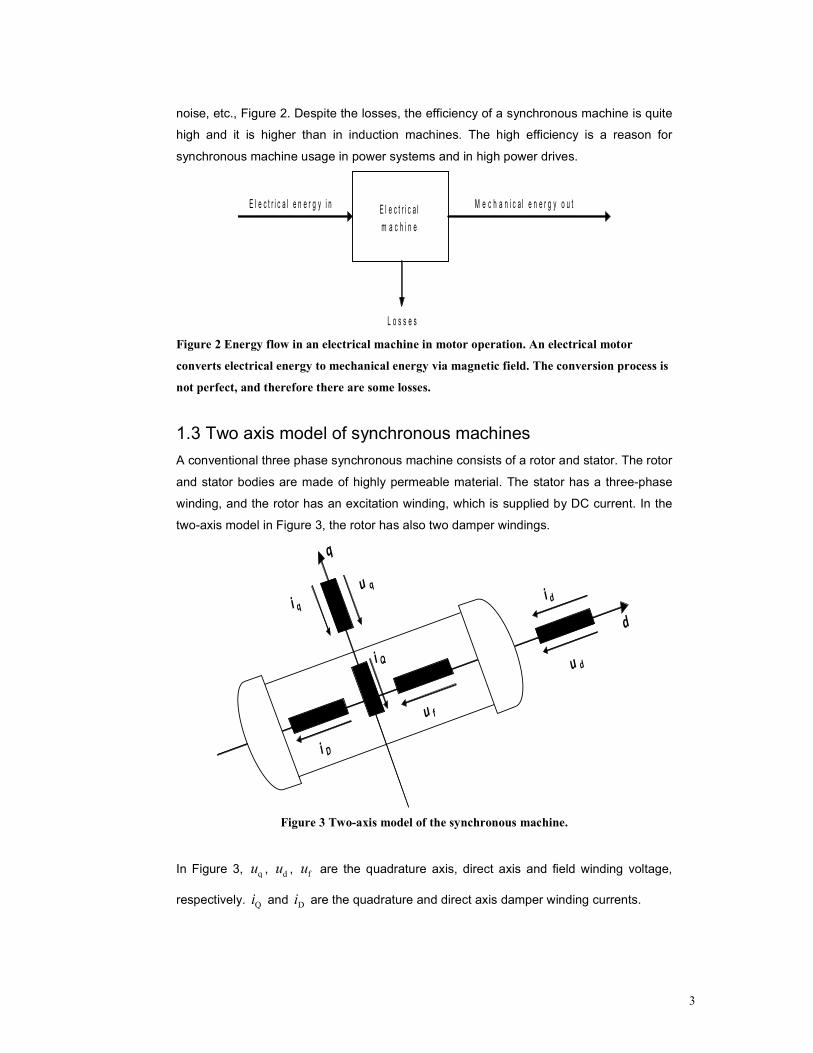
noise, etc., Figure 2. Despite the losses, the efficiency of a synchronous machine is quite
high and it is higher than in induction machines. The high efficiency is a reason for
synchronous machine usage in power systems and in high power drives.
E l e c t r i c a l
m a c h i n e
E l e c t r i c a l e n e r g y i n M e c h a n i c a l e n e r g y o u t
L o s s e s
Figure 2 Energy flow in an electrical machine in motor operation. An electrical motor
converts electrical energy to mechanical energy via magnetic field. The conversion process is
not perfect, and therefore there are some losses.
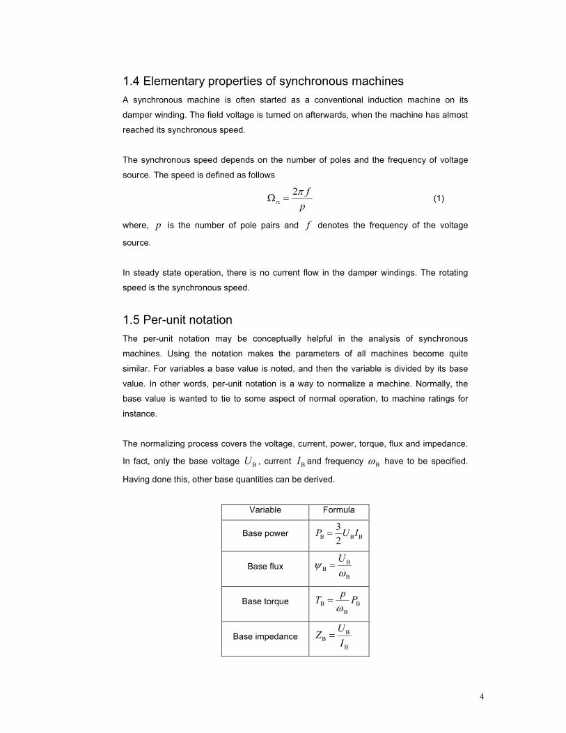
1.3 Two axis model of synchronous machines
A conventional three phase synchronous machine consists of a rotor and stator. The rotor
and stator bodies are made of highly permeable material. The stator has a three-phase
winding, and the rotor has an excitation winding, which is supplied by DC current. In the
two-axis model in Figure 3, the rotor has also two damper windings.
d
q
u d
u q
u f
i D
i qi d
i Q
Figure 3 Two-axis model of the synchronous machine.
In Figure 3, qu , du , fu are the quadrature axis, direct axis and field winding voltage,
respectively. Qi and Di are the quadrature and direct axis damper winding currents.
4
1.4 Elementary properties of synchronous machines
A synchronous machine is often started as a conventional induction machine on its
damper winding. The field voltage is turned on afterwards, when the machine has almost
reached its synchronous speed.
The synchronous speed depends on the number of poles and the frequency of voltage
source. The speed is defined as follows
2 f
pΩ =
m
π (1)
where, p is the number of pole pairs and f denotes the frequency of the voltage
source.
In steady state operation, there is no current flow in the damper windings. The rotating
speed is the synchronous speed.
1.5 Per-unit notation
The per-unit notation may be conceptually helpful in the analysis of synchronous
machines. Using the notation makes the parameters of all machines become quite
similar. For variables a base value is noted, and then the variable is divided by its base
value. In other words, per-unit notation is a way to normalize a machine. Normally, the
base value is wanted to tie to some aspect of normal operation, to machine ratings for
instance.
The normalizing process covers the voltage, current, power, torque, flux and impedance.
In fact, only the base voltage BU , current
BI and frequency Bω have to be specified.
Having done this, other base quantities can be derived.
Variable Formula
Base power B B B
3
2P U I=
Base flux B
B
B
U=ψω
Base torque B B
B
pT P
ω=
Base impedance B
B
B
UZ
I=
5
2 Methods
2.1 Simulation model
The use of the two-axis model is a conventional way to simulate synchronous machines.
The idea behind the model is to divide all variables into two axes. They are perpendicular
to each other, and therefore, there is no interaction. The rotor of a salient-pole
synchronous machine is asymmetric, and therefore equations are considered in a
system, which is rotating at rotor speed. Commonly, quantities, such as voltages and
currents, are referred to the stator.
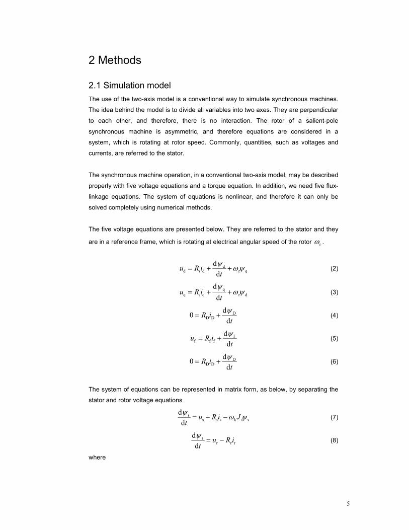
The synchronous machine operation, in a conventional two-axis model, may be described
properly with five voltage equations and a torque equation. In addition, we need five flux-
linkage equations. The system of equations is nonlinear, and therefore it can only be
solved completely using numerical methods.
The five voltage equations are presented below. They are referred to the stator and they
are in a reference frame, which is rotating at electrical angular speed of the rotor rω .
dd s d r q
d
du R i
t
ψωψ= + + (2)
q
q s q r d
d
du R i
t
ψωψ= + + (3)
DD D
d0
dR i
t
ψ= + (4)
ff f f
d
du R i
t
ψ= + (5)
DD D
d0
dR i
t
ψ= + (6)
The system of equations can be represented in matrix form, as below, by separating the
stator and rotor voltage equations
ss s s k s s
d
du R i J
t
ψω ψ= − − (7)
rr r r
d
du R i
t
ψ= − (8)
where
6
d
s
q
ψψ
ψ
=
d
s
q
uu
u
=
d
s
q
0
0
RR
R
=
d
s
q
ii
i
=
d
s
q
ii
i
=
s
0 1
1 0J
− =
and
f
r D
Q
ψψ ψ
ψ
=
f
r 0
0
u
u
=
f
r D
Q
0 0
0 0
0 0
R
R R
R
=
f
r D
Q
i
i i
i
=
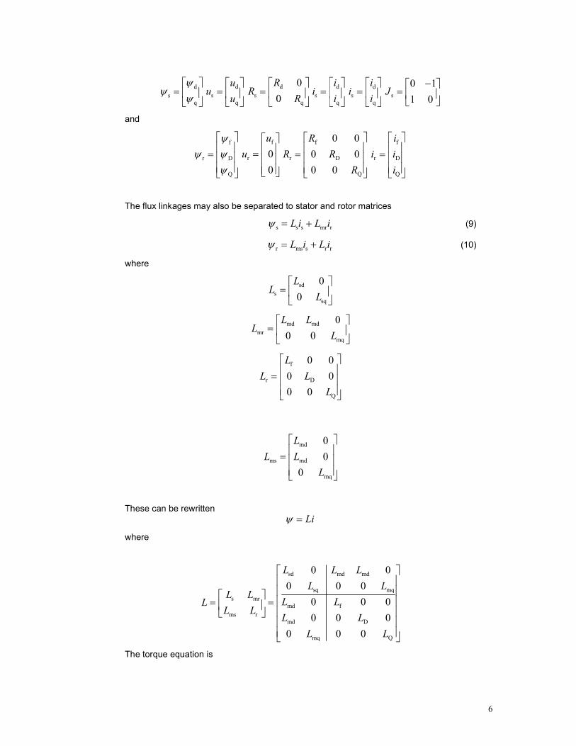
The flux linkages may also be separated to stator and rotor matrices
s s s mr rL i L iψ = + (9)
r ms s r rL i L iψ = + (10)
where
sd
s
sq
0
0
LL
L
=
md md
mr
mq
0
0 0
L LL
L
=
f
r D
Q
0 0
0 0
0 0
L
L L
L
=
md
ms md
mq
0
0
0
L
L L
L
=
These can be rewritten
Liψ =
where
sd md md
sq mq
s mr
md f
ms r
md D
mq Q
0 0
0 0 0
0 0 0
0 0 0
0 0 0
L L L
L LL L
L LLL L
L L
L L
= =
The torque equation is
7
e m
d
d
ω= +
JT T
p t (11)
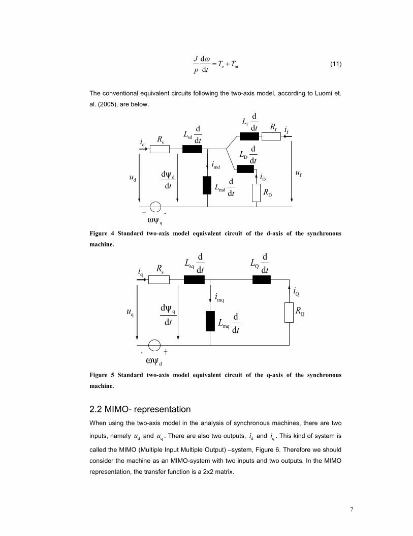
The conventional equivalent circuits following the two-axis model, according to Luomi et.
al. (2005), are below.
du
qωψ-+
sR
DR
fR
sd
d
dL
t
f
d
dL
t
D
d
dL
t
md
d
dL
t
fu
di
Di
fi
dd
dt
ψ
mdi
Figure 4 Standard two-axis model equivalent circuit of the d-axis of the synchronous
machine.
qu
dωψ+-
sR
QR
sq
d
dL
tQ
d
dL
t
mq
d
dL
t
qi
Qi
qd
dt
ψ
mqi
Figure 5 Standard two-axis model equivalent circuit of the q-axis of the synchronous
machine.
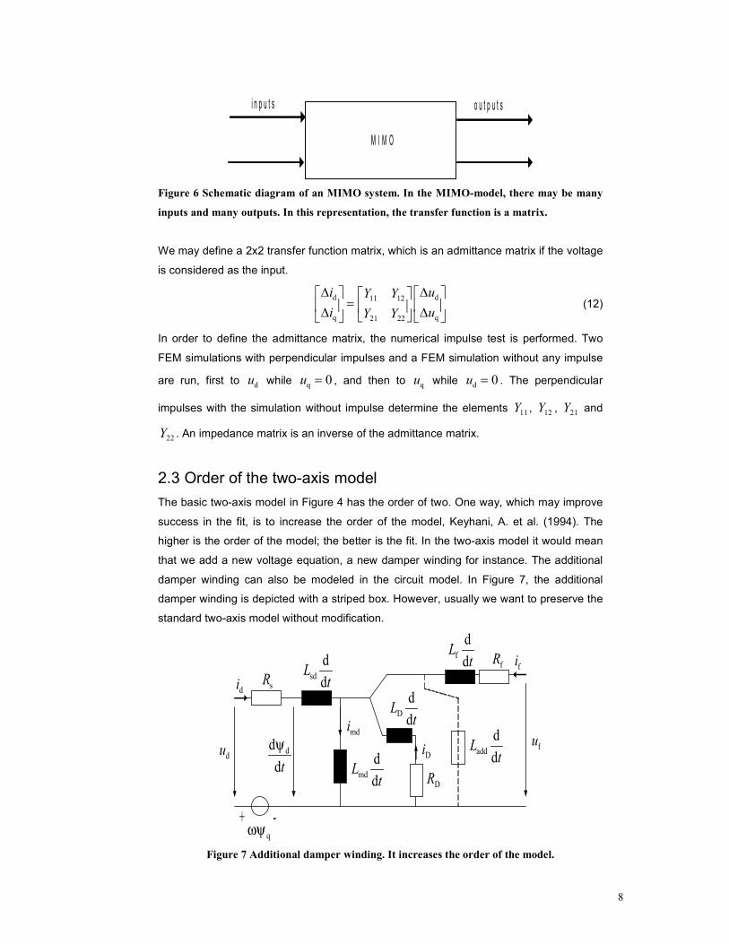
2.2 MIMO- representation
When using the two-axis model in the analysis of synchronous machines, there are two
inputs, namely du and qu . There are also two outputs, di and qi . This kind of system is
called the MIMO (Multiple Input Multiple Output) –system, Figure 6. Therefore we should
consider the machine as an MIMO-system with two inputs and two outputs. In the MIMO
representation, the transfer function is a 2x2 matrix.
8
M I M O
i n p u t s o u t p u t s
Figure 6 Schematic diagram of an MIMO system. In the MIMO-model, there may be many
inputs and many outputs. In this representation, the transfer function is a matrix.
We may define a 2x2 transfer function matrix, which is an admittance matrix if the voltage
is considered as the input.
d d11 12
q q21 22
i uY Y
i uY Y
∆ ∆ = ∆ ∆
(12)
In order to define the admittance matrix, the numerical impulse test is performed. Two
FEM simulations with perpendicular impulses and a FEM simulation without any impulse
are run, first to du while q 0u = , and then to qu while d 0u = . The perpendicular
impulses with the simulation without impulse determine the elements 11Y , 12Y , 21Y and
22Y . An impedance matrix is an inverse of the admittance matrix.
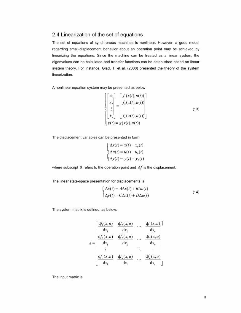
2.3 Order of the two-axis model
The basic two-axis model in Figure 4 has the order of two. One way, which may improve
success in the fit, is to increase the order of the model, Keyhani, A. et al. (1994). The
higher is the order of the model; the better is the fit. In the two-axis model it would mean
that we add a new voltage equation, a new damper winding for instance. The additional
damper winding can also be modeled in the circuit model. In Figure 7, the additional
damper winding is depicted with a striped box. However, usually we want to preserve the
standard two-axis model without modification.
du
qωψ-+
sR
DR
fR
sd
d
dL
t
f
d
dL
t
D
d
dL
t
md
d
dL
t
fu
di
Di
fi
dd
dt
ψ
mdi
add
d
dL
t
Figure 7 Additional damper winding. It increases the order of the model.
9
2.4 Linearization of the set of equations
The set of equations of synchronous machines is nonlinear. However, a good model
regarding small-displacement behavior about an operation point may be achieved by
linearizing the equations. Since the machine can be treated as a linear system, the
eigenvalues can be calculated and transfer functions can be established based on linear
system theory. For instance, Glad, T. et al. (2000) presented the theory of the system
linearization.
A nonlinear equation system may be presented as below
1 1
2 2
n n
( ( ), ( ))
( ( ), ( ))
( ( ), ( ))
( ) ( ( ), ( ))
= =
ɺ
ɺ
⋮ ⋮
ɺ
x f x t u t
x f x t u t
x f x t u t
y t g x t u t
(13)
The displacement variables can be presented in form
0
0
0
( ) ( ) ( )
( ) ( ) ( )
( ) ( ) ( )
x t x t x t
u t u t u t
y t y t y t
∆ = −∆ = −∆ = −
where subscript 0 refers to the operation point and f∆ is the displacement.
The linear state-space presentation for displacements is
( ) ( ) ( )
( ) ( ) ( )
x t A x t B u t
y t C x t D u t
∆ = ∆ + ∆∆ = ∆ + ∆
ɺ (14)
The system matrix is defined, as below,
1 2 1
1 2
2 2 2
1 2
n n n
1 1 n
d ( , ) d ( , ) d ( , )
d d d
d ( , ) d ( , ) d ( , )
d d d
d ( , ) d ( , ) d ( , )
d d d
=
⋯
⋯
⋮ ⋱ ⋮
⋯
n
n
f x u f x u f x u
x x x
f x u f x u f x u
x x xA
f x u f x u f x u
x x x
The input matrix is
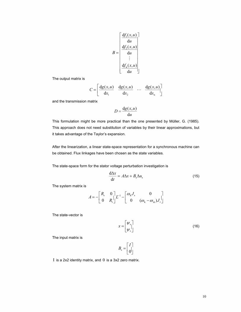
10
1
2
n
d ( , )
d
d ( , )
d
d ( , )
d
f x u
u
f x u
B u
f x u
u
=
⋮
The output matrix is
1 2 n
d ( , ) d ( , ) d ( , )
d d d
g x u g x u g x uC
x x x
=
⋯
and the transmission matrix
d ( , )
d
g x uD
u=
This formulation might be more practical than the one presented by Müller, G. (1985).
This approach does not need substitution of variables by their linear approximations, but
it takes advantage of the Taylor’s expansion.
After the linearization, a linear state-space representation for a synchronous machine can
be obtained. Flux linkages have been chosen as the state variables.
The state-space form for the stator voltage perturbation investigation is
s s
d
d
xA x B u
t
∆= ∆ + ∆ (15)
The system matrix is
s k s1
r k m r
0 0
0 0 ( )
R JA L
R J
ωω ω
− = − − −
The state-vector is
s
r
xψψ
=
(16)
The input matrix is
s0
IB
=
I is a 2x2 identity matrix, and 0 is a 3x2 zero matrix.
11
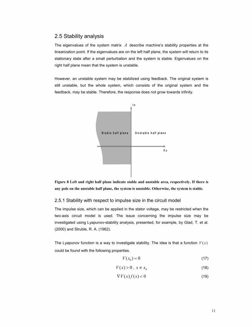
2.5 Stability analysis
The eigenvalues of the system matrix A describe machine’s stability properties at the
linearization point. If the eigenvalues are on the left half plane, the system will return to its
stationary state after a small perturbation and the system is stable. Eigenvalues on the
right half plane mean that the system is unstable.
However, an unstable system may be stabilized using feedback. The original system is
still unstable, but the whole system, which consists of the original system and the
feedback, may be stable. Therefore, the response does not grow towards infinity.
R e
I m
U n s t a b l e h a l f p l a n eS t a b l e h a l f p l a n e
Figure 8 Left and right half plane indicate stable and unstable area, respectively. If there is
any pole on the unstable half plane, the system is unstable. Otherwise, the system is stable.
2.5.1 Stability with respect to impulse size in the circuit model
The impulse size, which can be applied in the stator voltage, may be restricted when the
two-axis circuit model is used. The issue concerning the impulse size may be
investigated using Lyapunov-stability analysis, presented, for example, by Glad, T. et al.
(2000) and Struble, R. A. (1962).
The Lyapunov function is a way to investigate stability. The idea is that a function ( )V x
could be found with the following properties.
0( ) 0V x = (17)
( ) 0V x > , 0x x≠ (18)
( ) ( ) 0V x f x∇ < (19)
12
( )f x is presented in Equation 13. An arbitrary point can be interpreted as a point at
origin by making a coordinate transform. Therefore, the stability study at the origin is
sufficient. At the origin, the input is zero.
One may consider stator voltage as the input. The voltage equation for the stator
d d d
s k
q q q
0 1d
1 0d
iRit
ψ ψω
ψ ψ−
= − −
Using substitutiond 1
q 2
ψ
ψ
=
x
x, the set of equations above may be formulated, as
follows,
1
1 s d 1 k 2
1
2 s q 2 k 1
ωω
−
−
= − +
= − −
ɺ
ɺ
x R L x x
x R L x x
We may try a Lyapunov function, which has the following form
2 2
1 2( )V x x xα= + , 0α >
then holds ( ) 0V x > , when 0x x≠ and 0( ) 0V x = when 0 0x x= =
[ ]1 2( ) 2 2V x x xα∇ =
1 1
1 s d 1 1 k 2 2 s q 2 2 k 1( ) ( ) 2 2 2 2V x f x x R L x x x x R L x x xα α ω ω− −∇ = − + − −
Choosing 1α = one gets
1 2 1 2
s d 1 s q 2( ) ( ) 2 2 0V x f x R L x R L x− −∇ = − − <
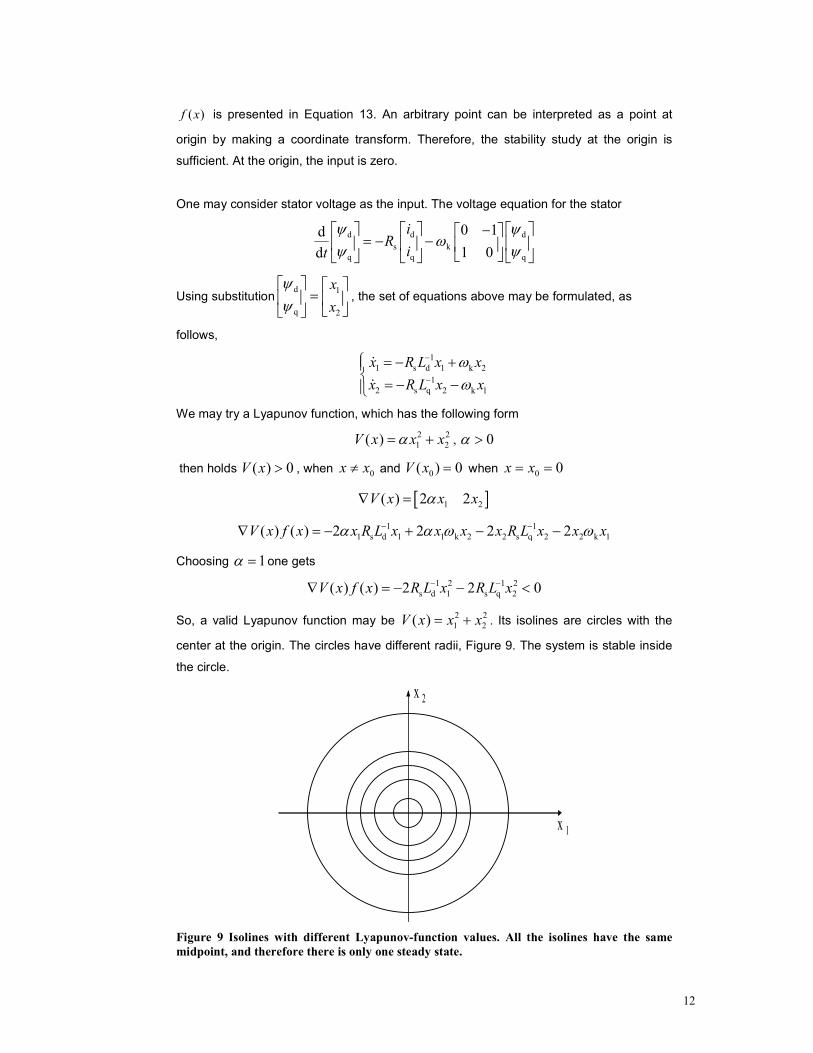
So, a valid Lyapunov function may be 2 2
1 2( )V x x x= + . Its isolines are circles with the
center at the origin. The circles have different radii, Figure 9. The system is stable inside
the circle.
x 1
x 2
Figure 9 Isolines with different Lyapunov-function values. All the isolines have the same
midpoint, and therefore there is only one steady state.
13
A system is globally asymptotically stable if there is a function V, additional to Eq. 17-19,
satisfying
( ) ,V x →∞ when x →∞
If we are considering a circuit model, the impulse size does not affect to the operation
point. There is only one steady state. The system is stable in the sense of Lyapunov, and
the system will always return to its steady state. The return time depends on the
eigenvalues of the system matrix. The further on the left half plane the eigenvalues are,
the faster the machine returns to its steady state.
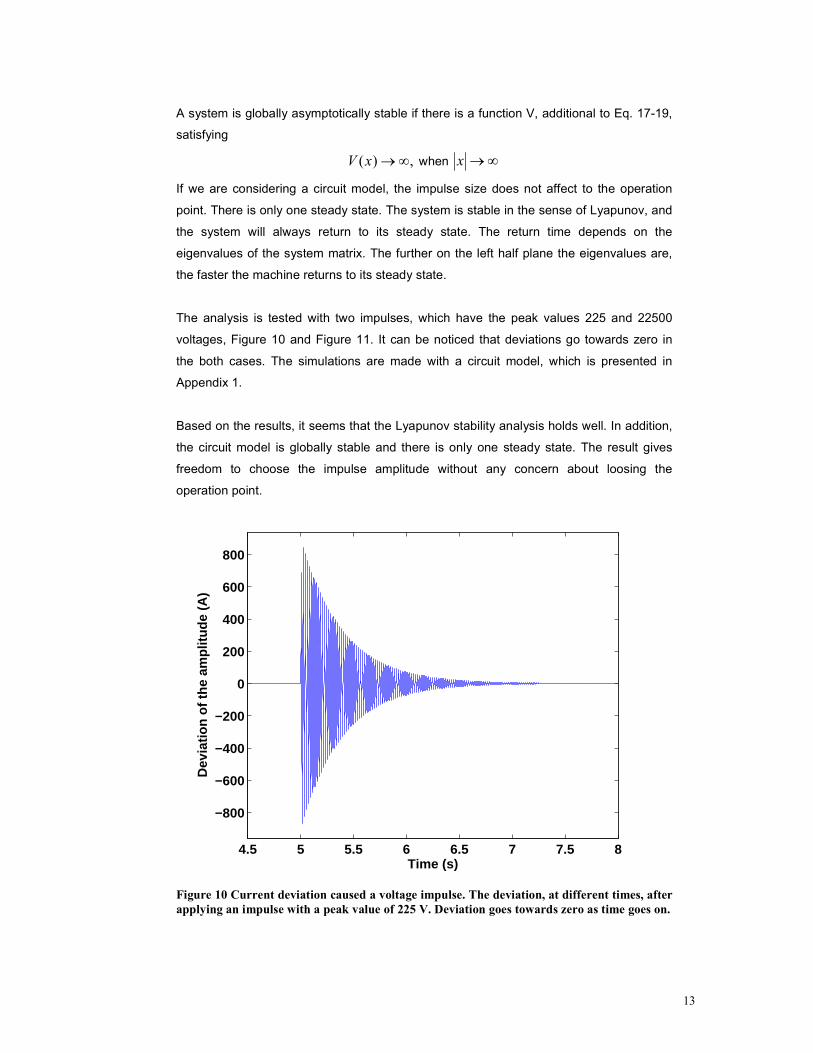
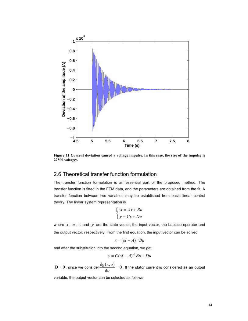
The analysis is tested with two impulses, which have the peak values 225 and 22500
voltages, Figure 10 and Figure 11. It can be noticed that deviations go towards zero in
the both cases. The simulations are made with a circuit model, which is presented in
Appendix 1.
Based on the results, it seems that the Lyapunov stability analysis holds well. In addition,
the circuit model is globally stable and there is only one steady state. The result gives
freedom to choose the impulse amplitude without any concern about loosing the
operation point.
4.5 5 5.5 6 6.5 7 7.5 8
−800
−600
−400
−200
0
200
400
600
800
Time (s)
Dev
iatio
n of
the
ampl
itude
(A
)
Figure 10 Current deviation caused a voltage impulse. The deviation, at different times, after
applying an impulse with a peak value of 225 V. Deviation goes towards zero as time goes on.
14
4.5 5 5.5 6 6.5 7 7.5 8−1
−0.8
−0.6
−0.4
−0.2
0
0.2
0.4
0.6
0.8
1x 10
5
Time (s)
Dev
iatio
n of
the
ampl
itude
(A
)
Figure 11 Current deviation caused a voltage impulse. In this case, the size of the impulse is
22500 voltages.
2.6 Theoretical transfer function formulation
The transfer function formulation is an essential part of the proposed method. The
transfer function is fitted in the FEM data, and the parameters are obtained from the fit. A
transfer function between two variables may be established from basic linear control
theory. The linear system representation is
sx Ax Bu
y Cx Du
= +
= +
where x , u , s and y are the state vector, the input vector, the Laplace operator and
the output vector, respectively. From the first equation, the input vector can be solved
1(s )x I A Bu−= −
and after the substitution into the second equation, we get
1(s )y C I A Bu Du−= − +
0D = , since we considerd ( , )
0d
g x u
u= . If the stator current is considered as an output
variable, the output vector can be selected as follows
15
d
s s
q
iy i C x
i
= = =
where
[ ] 1
s 0C I L−=
x is the state vector, s
r
xψψ
=
For instance, a transfer function between stator current and voltage may be presented as
follows
s s si Y u=
1
s s s( ) ( )Y s C sI A B−= −
where, s0
IB
=
This kind of transfer function formulation is more efficient than the one presented by
Krause et al. (2002). The formulation presented by Krause needs a matrix inversion for a
5x5 matrix three times, whereas the above formulation only once. Therefore, this
approach is computationally more efficient.
2.7 Numerical transfer function
The numerical transfer function is established from the time-stepping FEM data. The
purpose of the numerical transfer function is to give the estimation data for wherein the
theoretical transfer function is fitted. Normally the transfer function is considered in
frequency domain, and the Fourier transform makes the transformation from the time to
frequency domain. In the frequency domain, the transfer function may be presented, as
follows
( j )( j )
( j )
YG
U
ωω
ω=
( j )Y ω and ( j )U ω are the input and output data in frequency domain, respectively. The
transfer function ( j )G ω is also called the frequency response function. It depicts the
spectral properties of the system.
16
The input should include all desired frequencies in order to take all time constants into
account. Different inputs produce different outputs, but the ratio is always constant. The
ratio is the numerical transfer function.
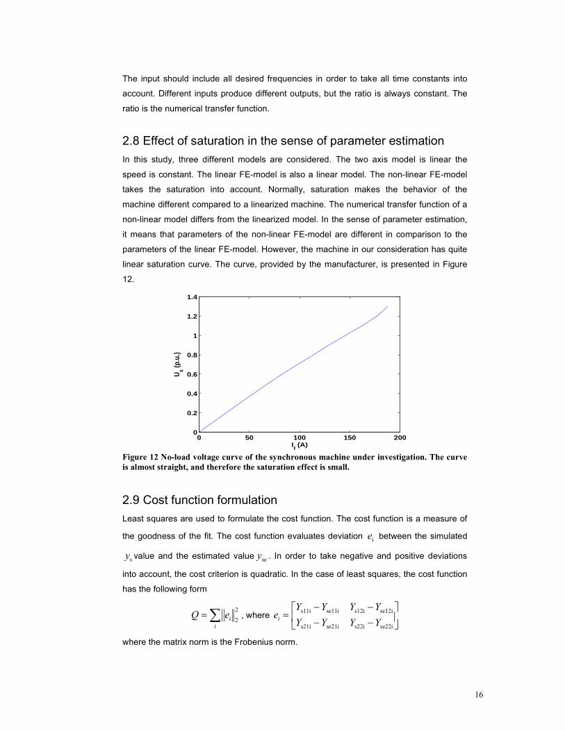
2.8 Effect of saturation in the sense of parameter estimation
In this study, three different models are considered. The two axis model is linear the
speed is constant. The linear FE-model is also a linear model. The non-linear FE-model
takes the saturation into account. Normally, saturation makes the behavior of the
machine different compared to a linearized machine. The numerical transfer function of a
non-linear model differs from the linearized model. In the sense of parameter estimation,
it means that parameters of the non-linear FE-model are different in comparison to the
parameters of the linear FE-model. However, the machine in our consideration has quite
linear saturation curve. The curve, provided by the manufacturer, is presented in Figure
12.
0 50 100 150 2000
0.2
0.4
0.6
0.8
1
1.2
1.4
If (A)
Us (p
.u.)
Figure 12 No-load voltage curve of the synchronous machine under investigation. The curve
is almost straight, and therefore the saturation effect is small.
2.9 Cost function formulation
Least squares are used to formulate the cost function. The cost function is a measure of
the goodness of the fit. The cost function evaluates deviation ie between the simulated
sy value and the estimated value sey . In order to take negative and positive deviations
into account, the cost criterion is quadratic. In the case of least squares, the cost function
has the following form
2
i 2i
Q e=∑ , where s11i se11i s12i se12i
s21i se21i s22i se22i
i
Y Y Y Ye
Y Y Y Y
− − = − −
where the matrix norm is the Frobenius norm.
17
2.10 Differential Evolution algorithm
The Differential Evolution algorithm makes the minimization of the cost function. The
algorithm is a global optimization method that is based on evolution strategies. Price et al.
(2005) presented the theory and practice of the Differential Evolution algorithm in their
book.
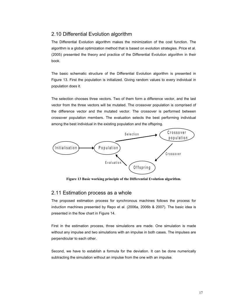
The basic schematic structure of the Differential Evolution algorithm is presented in
Figure 13. First the population is initialized. Giving random values to every individual in
population does it.
The selection chooses three vectors. Two of them form a difference vector, and the last
vector from the three vectors will be mutated. The crossover population is comprised of
the difference vector and the mutated vector. The crossover is performed between
crossover population members. The evaluation selects the best performing individual
among the best individual in the existing population and the offspring.
P o p u l a t i o nI n i t i a l i s a t i o n
C r o s s o v e r
p o p u l a t i o n
O f f s p r i n g
S e l e c t i o n
E v a l u a t i o n
C r o s s o v e r
Figure 13 Basic working principle of the Differential Evolution algorithm.
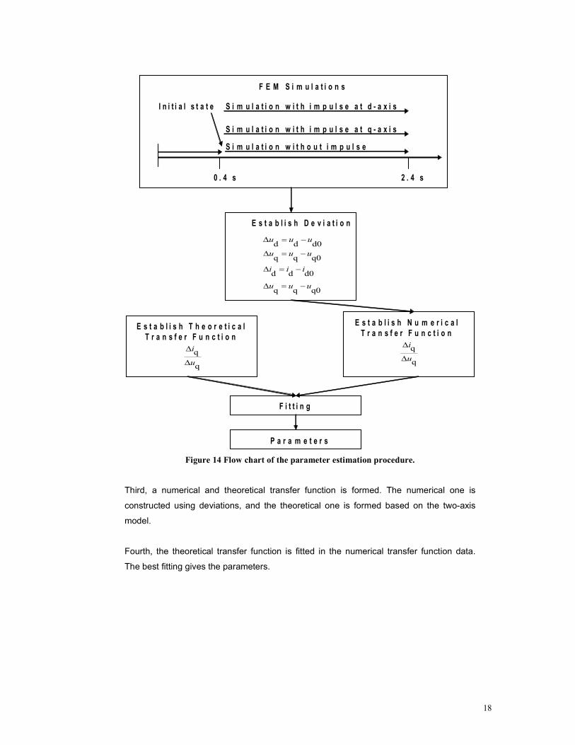
2.11 Estimation process as a whole
The proposed estimation process for synchronous machines follows the process for
induction machines presented by Repo et al. (2006a, 2006b & 2007). The basic idea is
presented in the flow chart in Figure 14.
First in the estimation process, three simulations are made. One simulation is made
without any impulse and two simulations with an impulse in both cases. The impulses are
perpendicular to each other.
Second, we have to establish a formula for the deviation. It can be done numerically
subtracting the simulation without an impulse from the one with an impulse.
18
0 . 4 s 2 . 4 s
I n i t i a l s t a t e
S i m u l a t i o n w i t h o u t i m p u l s e
S i m u l a t i o n w i t h i m p u l s e a t q - a x i s
S i m u l a t i o n w i t h i m p u l s e a t d - a x i s
E s t a b l i s h D e v i a t i o n
d d d0∆ = −u u u
q q q0∆ = −u u u
d d d0∆ = −i i i
q q q0∆ = −u u u
E s t a b l i s h N u m e r i c a l
T r a n s f e r F u n c t i o n
q
q
∆
∆
i
u
E s t a b l i s h T h e o r e t i c a l
T r a n s f e r F u n c t i o n
q
q
∆
∆
i
u
F i t t i n g
P a r a m e t e r s
F E M S i m u l a t i o n s
Figure 14 Flow chart of the parameter estimation procedure.
Third, a numerical and theoretical transfer function is formed. The numerical one is
constructed using deviations, and the theoretical one is formed based on the two-axis
model.
Fourth, the theoretical transfer function is fitted in the numerical transfer function data.
The best fitting gives the parameters.
19
3 Results
3.1 Introduction
The machine under study is a 6-pole, Y-connected three-phase synchronous motor. The
rated values are 12.5 MW, 3150V, 1-power factor, 50 Hz, and 1000 r/min.
In this study, the excitation is applied into stator voltage and the stator current response is
recorded. The simulations are made with the FEM and for verification purposes with the
circuit model. The FEM-simulations are made with a linear and non-linear machine
model. In other words, we can consider the difference of results between the linear and
non-linear machine models.
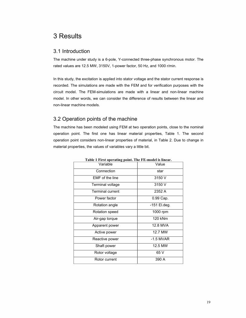
3.2 Operation points of the machine
The machine has been modeled using FEM at two operation points, close to the nominal
operation point. The first one has linear material properties, Table 1. The second
operation point considers non-linear properties of material, in Table 2. Due to change in
material properties, the values of variables vary a little bit.
Table 1 First operating point. The FE-model is linear.
Variable Value
Connection star
EMF of the line 3150 V
Terminal voltage 3150 V
Terminal current 2352 A
Power factor 0.99 Cap.
Rotation angle -151 El.deg.
Rotation speed 1000 rpm
Air-gap torque 120 kNm
Apparent power 12.8 MVA
Active power 12.7 MW
Reactive power -1.5 MVAR
Shaft power 12.5 MW
Rotor voltage 65 V
Rotor current 390 A
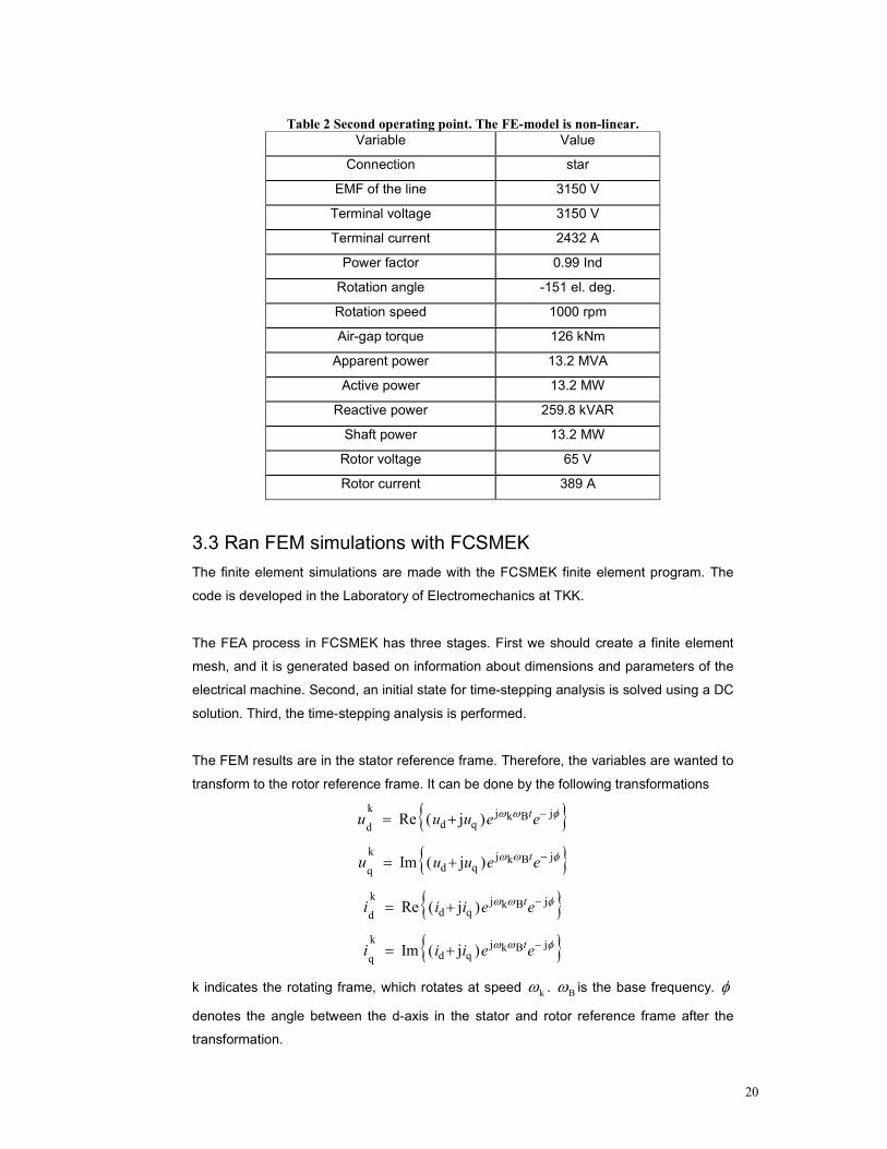
20
Table 2 Second operating point. The FE-model is non-linear.
Variable Value
Connection star
EMF of the line 3150 V
Terminal voltage 3150 V
Terminal current 2432 A
Power factor 0.99 Ind
Rotation angle -151 el. deg.
Rotation speed 1000 rpm
Air-gap torque 126 kNm
Apparent power 13.2 MVA
Active power 13.2 MW
Reactive power 259.8 kVAR
Shaft power 13.2 MW
Rotor voltage 65 V
Rotor current 389 A
3.3 Ran FEM simulations with FCSMEK
The finite element simulations are made with the FCSMEK finite element program. The
code is developed in the Laboratory of Electromechanics at TKK.
The FEA process in FCSMEK has three stages. First we should create a finite element
mesh, and it is generated based on information about dimensions and parameters of the
electrical machine. Second, an initial state for time-stepping analysis is solved using a DC
solution. Third, the time-stepping analysis is performed.
The FEM results are in the stator reference frame. Therefore, the variables are wanted to
transform to the rotor reference frame. It can be done by the following transformations
k j jk Bd qd
Re ( j ) tu u e eu ω ω φ−= +
k j jk Bd qq
Im ( j ) tu u e eu ω ω φ−= +
k j jk Bd qd
Re ( j ) ti i e ei ω ω φ−= +
k j jk Bd qq
Im ( j )t
i i e ei ω ω φ−= +
k indicates the rotating frame, which rotates at speed kω . Bω is the base frequency. φ
denotes the angle between the d-axis in the stator and rotor reference frame after the
transformation.
21
φ
d r d s
q r
q s
Figure 15 Angle between d-axis in stator and rotor’s reference frame is defined to be φ .
rq , sq and rd , sd depict the q-axis and d-axis in the rotor and stator reference frame,
respectively.
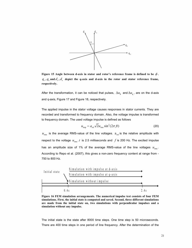
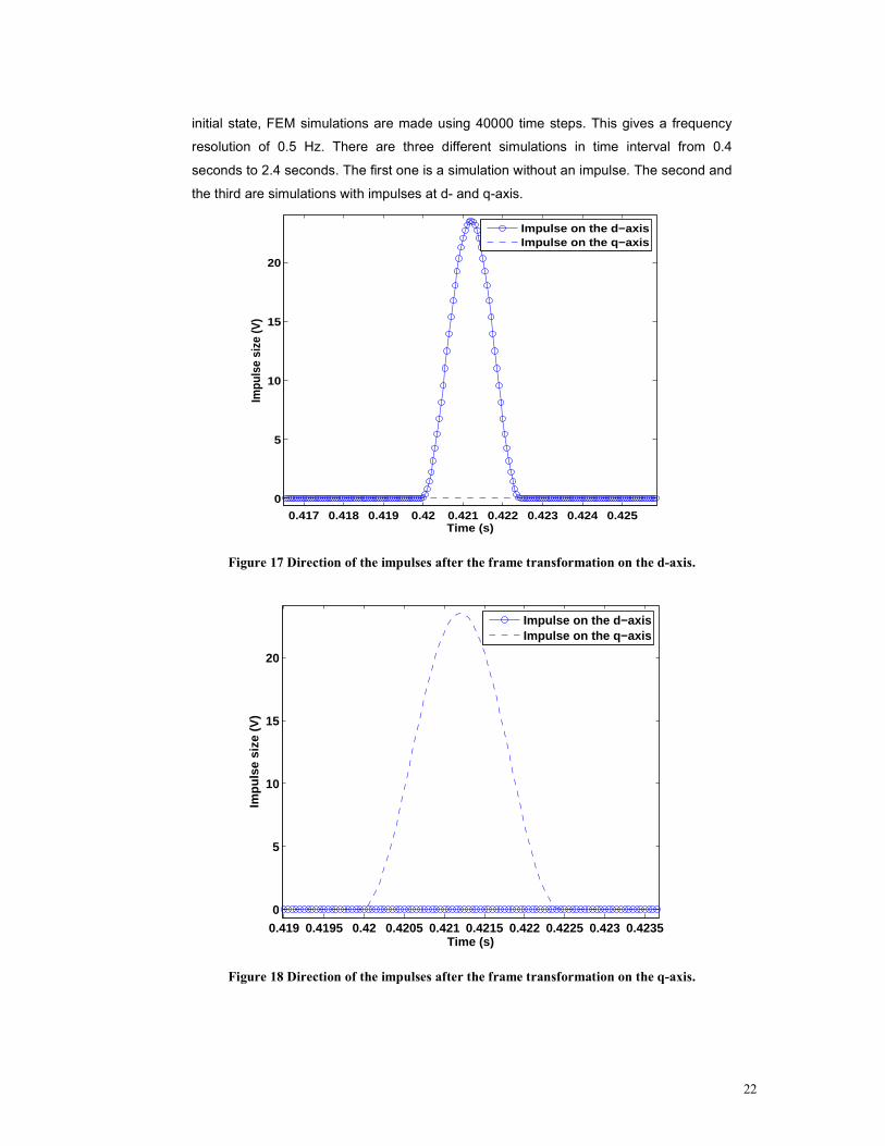
After the transformation, it can be noticed that pulses, du∆ and qu∆ , are on the d-axis
and q-axis, Figure 17 and Figure 18, respectively.
The applied impulse in the stator voltage causes responses in stator currents. They are
recorded and transformed to frequency domain. Also, the voltage impulse is transformed
to frequency domain. The used voltage impulse is defined as follows
2
imp rel rms2 sin (2 )u a u ftπ= (20)
rmsu is the average RMS-value of the line voltages. rela is the relative amplitude with
respect to the voltage rmsu . t is 2.5 milliseconds and f is 200 Hz. The excited impulse
has an amplitude size of 1% of the average RMS-value of the line voltages rmsu .
According to Repo et al. (2007), this gives a non-zero frequency content at range from -
750 to 800 Hz.
0 . 4 s 2 . 4 s
I n i t i a l s t a t e
S i m u l a t i o n w i t h o u t i m p u l s e
S i m u l a t i o n w i t h i m p u l s e a t q - a x i s
S i m u l a t i o n w i t h i m p u l s e a t d - a x i s
Figure 16 FEM simulation arrangements. The numerical impulse test consists of four FEM
simulations. First, the initial state is computed and saved. Second, three different simulations
are made from the initial state on, two simulations with perpendicular impulses and a
simulation without any impulse.
The initial state is the state after 8000 time steps. One time step is 50 microseconds.
There are 400 time steps in one period of line frequency. After the determination of the
22
initial state, FEM simulations are made using 40000 time steps. This gives a frequency
resolution of 0.5 Hz. There are three different simulations in time interval from 0.4
seconds to 2.4 seconds. The first one is a simulation without an impulse. The second and
the third are simulations with impulses at d- and q-axis.
0.417 0.418 0.419 0.42 0.421 0.422 0.423 0.424 0.425
0
5
10
15
20
Time (s)
Impu
lse
size
(V)
Impulse on the d−axisImpulse on the q−axis
Figure 17 Direction of the impulses after the frame transformation on the d-axis.
0.419 0.4195 0.42 0.4205 0.421 0.4215 0.422 0.4225 0.423 0.42350
5
10
15
20
Time (s)
Impu
lse
size
(V
)
Impulse on the d−axisImpulse on the q−axis
Figure 18 Direction of the impulses after the frame transformation on the q-axis.
23
This kind of approach is profitable; we can subtract the simulations with and without
impulse from each other, and thus we can determine the deviation easily. The deviation
in response can be specified in the same way.
d d d0∆ = −u u u
q q q0∆ = −u u u
d d d0∆ = −i i i
q q q0∆ = −u u u
du denotes simulation with impulse, and d0u without impulse.
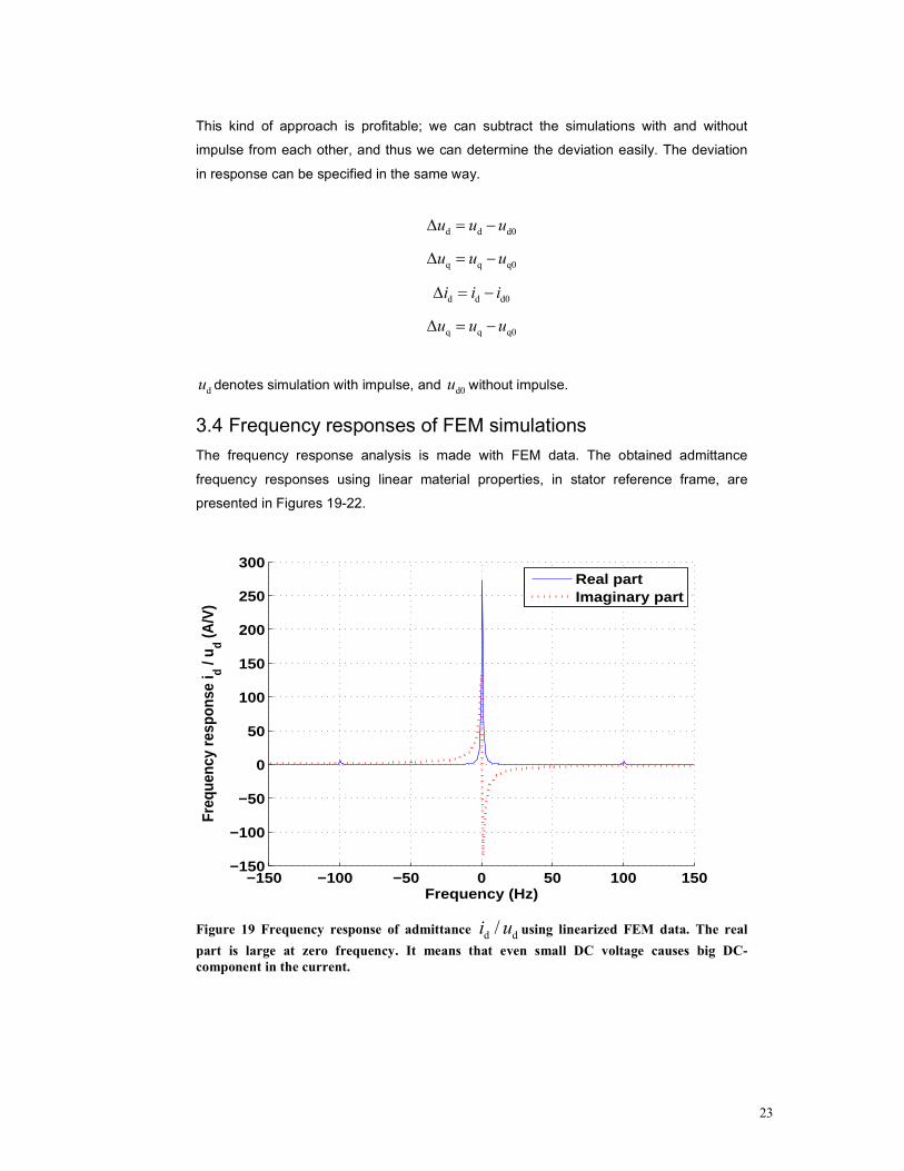
3.4 Frequency responses of FEM simulations
The frequency response analysis is made with FEM data. The obtained admittance
frequency responses using linear material properties, in stator reference frame, are
presented in Figures 19-22.
−150 −100 −50 0 50 100 150−150
−100
−50
0
50
100
150
200
250
300
Frequency (Hz)
Freq
uenc
y re
spon
se i
d / u d (A
/V)
Real partImaginary part
Figure 19 Frequency response of admittance d d/i u using linearized FEM data. The real
part is large at zero frequency. It means that even small DC voltage causes big DC-
component in the current.
24
−150 −100 −50 0 50 100 150−40
−30
−20
−10
0
10
20
Frequency (Hz)
Freq
uenc
y re
spon
se i
q / u d (A
/V)
Real partImaginary part
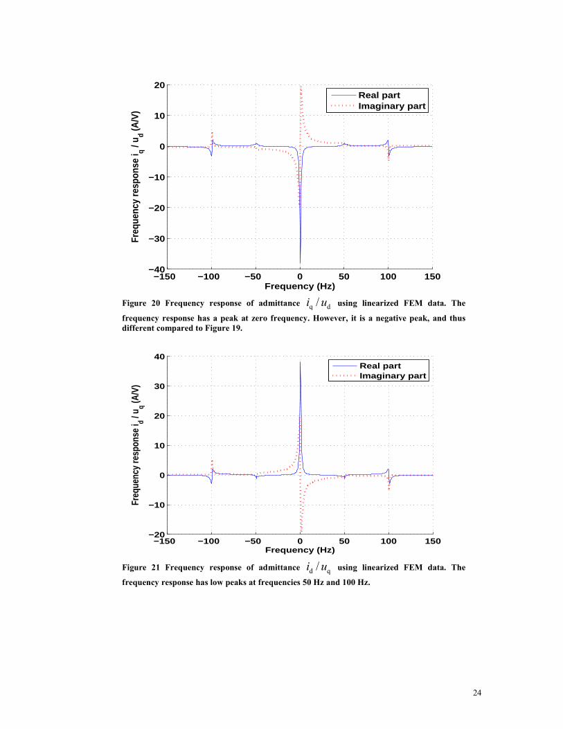
Figure 20 Frequency response of admittance q d/i u using linearized FEM data. The
frequency response has a peak at zero frequency. However, it is a negative peak, and thus
different compared to Figure 19.
−150 −100 −50 0 50 100 150−20
−10
0
10
20
30
40
Frequency (Hz)
Freq
uenc
y re
spon
se i
d / u q (A
/V)
Real partImaginary part
Figure 21 Frequency response of admittance d q/i u using linearized FEM data. The
frequency response has low peaks at frequencies 50 Hz and 100 Hz.
25
−150 −100 −50 0 50 100 150−150
−100
−50
0
50
100
150
200
250
300
Frequency (Hz)
Freq
uenc
y re
spon
se i
q / u q (A
/V)
Real partImaginary part
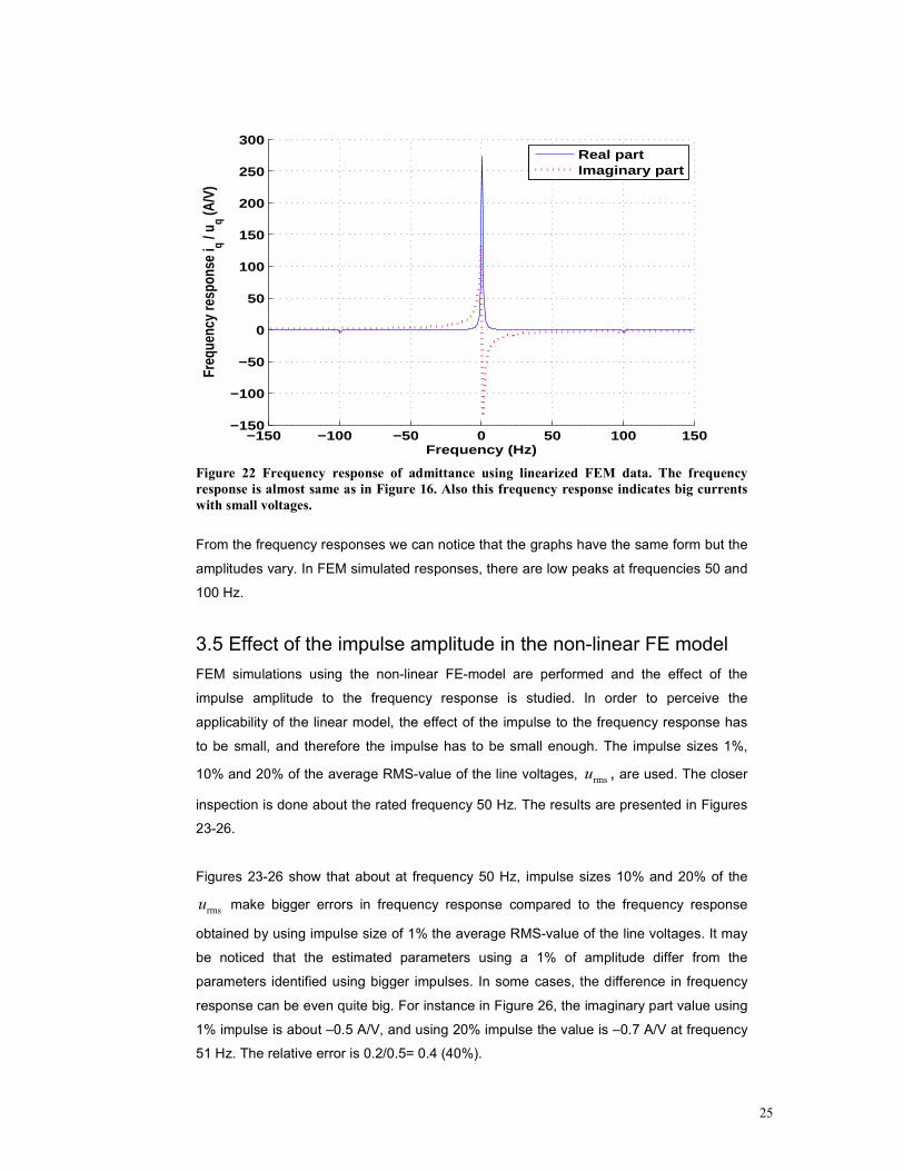
Figure 22 Frequency response of admittance using linearized FEM data. The frequency
response is almost same as in Figure 16. Also this frequency response indicates big currents
with small voltages.
From the frequency responses we can notice that the graphs have the same form but the
amplitudes vary. In FEM simulated responses, there are low peaks at frequencies 50 and
100 Hz.
3.5 Effect of the impulse amplitude in the non-linear FE model
FEM simulations using the non-linear FE-model are performed and the effect of the
impulse amplitude to the frequency response is studied. In order to perceive the
applicability of the linear model, the effect of the impulse to the frequency response has
to be small, and therefore the impulse has to be small enough. The impulse sizes 1%,
10% and 20% of the average RMS-value of the line voltages, rmsu , are used. The closer
inspection is done about the rated frequency 50 Hz. The results are presented in Figures
23-26.
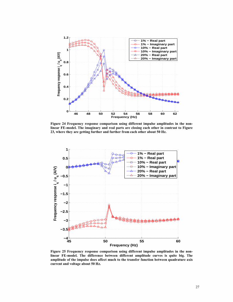
Figures 23-26 show that about at frequency 50 Hz, impulse sizes 10% and 20% of the
rmsu make bigger errors in frequency response compared to the frequency response
obtained by using impulse size of 1% the average RMS-value of the line voltages. It may
be noticed that the estimated parameters using a 1% of amplitude differ from the
parameters identified using bigger impulses. In some cases, the difference in frequency
response can be even quite big. For instance in Figure 26, the imaginary part value using
1% impulse is about –0.5 A/V, and using 20% impulse the value is –0.7 A/V at frequency
51 Hz. The relative error is 0.2/0.5= 0.4 (40%).
26
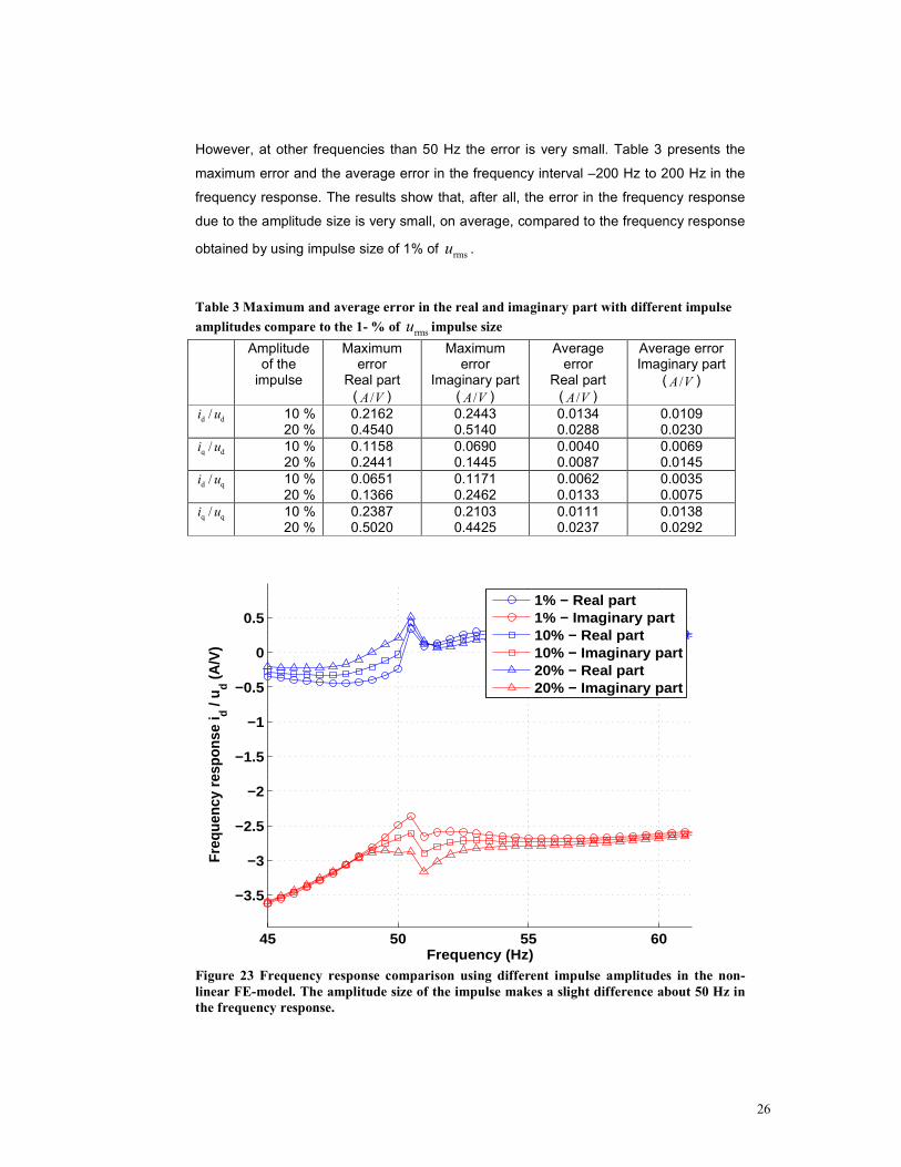
However, at other frequencies than 50 Hz the error is very small. Table 3 presents the
maximum error and the average error in the frequency interval –200 Hz to 200 Hz in the
frequency response. The results show that, after all, the error in the frequency response
due to the amplitude size is very small, on average, compared to the frequency response
obtained by using impulse size of 1% of rmsu .
Table 3 Maximum and average error in the real and imaginary part with different impulse
amplitudes compare to the 1- % of rmsu impulse size
Amplitude of the impulse
Maximum error
Real part
( /A V )
Maximum error
Imaginary part
( /A V )
Average error
Real part
( /A V )
Average error Imaginary part
( /A V )
d d/i u 10 % 20 %
0.2162 0.4540
0.2443 0.5140
0.0134 0.0288
0.0109 0.0230
q d/i u
10 % 20 %
0.1158 0.2441
0.0690 0.1445
0.0040 0.0087
0.0069 0.0145
d q/i u
10 % 20 %
0.0651 0.1366
0.1171 0.2462
0.0062 0.0133
0.0035 0.0075
q q/i u
10 % 20 %
0.2387 0.5020
0.2103 0.4425
0.0111 0.0237
0.0138 0.0292
45 50 55 60
−3.5
−3
−2.5
−2
−1.5
−1
−0.5
0
0.5
Frequency (Hz)
Freq
uenc
y re
spon
se i
d / u d (A
/V)
1% − Real part1% − Imaginary part10% − Real part10% − Imaginary part20% − Real part20% − Imaginary part
Figure 23 Frequency response comparison using different impulse amplitudes in the non-
linear FE-model. The amplitude size of the impulse makes a slight difference about 50 Hz in
the frequency response.
27
46 48 50 52 54 56 58 60 620
0.2
0.4
0.6
0.8
1
1.2
Frequency (Hz)
Freq
uenc
y re
spon
se i
q / u d (A
/V)
1% − Real part1% − Imaginary part10% − Real part10% − Imaginary part20% − Real part20% − Imaginary part
Figure 24 Frequency response comparison using different impulse amplitudes in the non-
linear FE-model. The imaginary and real parts are closing each other in contrast to Figure
23, where they are getting further and further from each other about 50 Hz.
45 50 55 60−4
−3.5
−3
−2.5
−2
−1.5
−1
−0.5
0
0.5
1
Frequency (Hz)
Freq
uenc
y re
spon
se i
q / u q (A
/V)
1% − Real part1% − Real part10% − Real part10% − Imaginary part20% − Real part20% − Imaginary part
Figure 25 Frequency response comparison using different impulse amplitudes in the non-
linear FE-model. The difference between different amplitude curves is quite big. The
amplitude of the impulse does affect much to the transfer function between quadrature axis
current and voltage about 50 Hz.
28
45 50 55 60−1.4
−1.2
−1
−0.8
−0.6
−0.4
−0.2
0
0.2
Frequency (Hz)
Freq
uenc
y re
spon
se i
d / u q (A
/V)
1% − Real part1% − Imaginary part10% − Real part10% − Imaginary part20% − Real part20% − Imaginary part
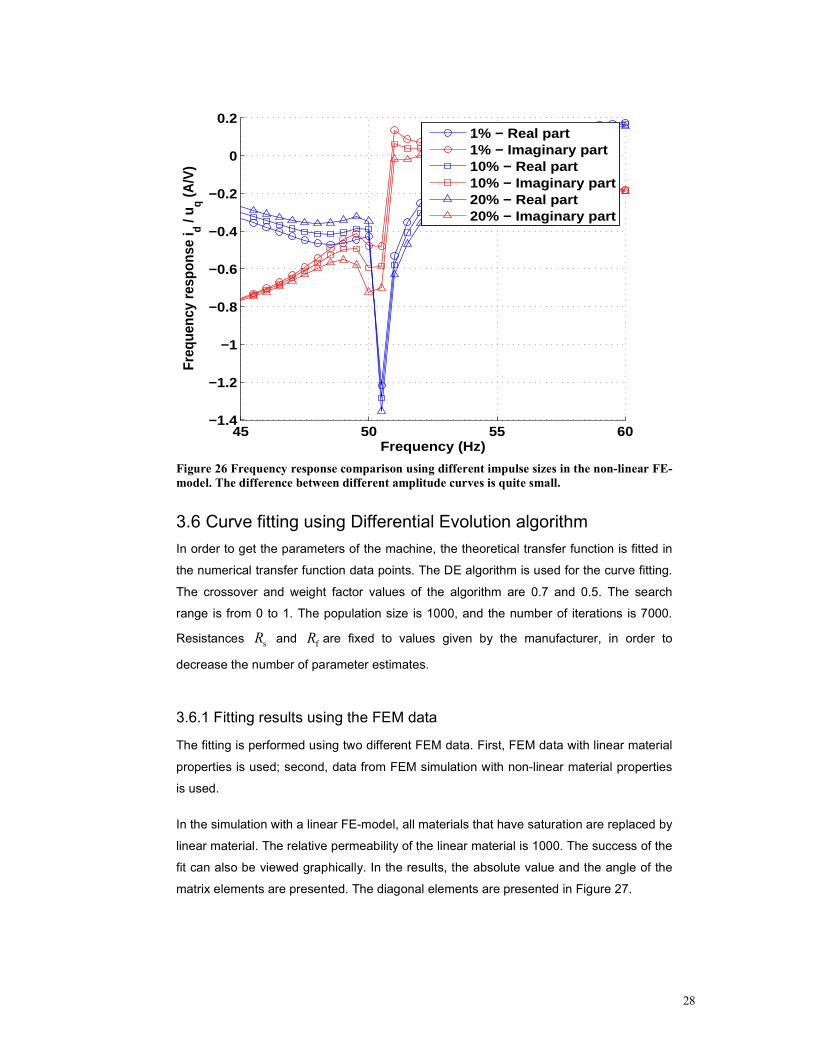
Figure 26 Frequency response comparison using different impulse sizes in the non-linear FE-
model. The difference between different amplitude curves is quite small.
3.6 Curve fitting using Differential Evolution algorithm
In order to get the parameters of the machine, the theoretical transfer function is fitted in
the numerical transfer function data points. The DE algorithm is used for the curve fitting.
The crossover and weight factor values of the algorithm are 0.7 and 0.5. The search
range is from 0 to 1. The population size is 1000, and the number of iterations is 7000.
Resistances sR and fR are fixed to values given by the manufacturer, in order to
decrease the number of parameter estimates.
3.6.1 Fitting results using the FEM data
The fitting is performed using two different FEM data. First, FEM data with linear material
properties is used; second, data from FEM simulation with non-linear material properties
is used.
In the simulation with a linear FE-model, all materials that have saturation are replaced by
linear material. The relative permeability of the linear material is 1000. The success of the
fit can also be viewed graphically. In the results, the absolute value and the angle of the
matrix elements are presented. The diagonal elements are presented in Figure 27.
29
0.1
1
|Z11
|,|Z 22
| (p.
u.)
0.1 1 30
90
180
∠ Z 11
, ∠ Z
22 (d
eg)
ω (p.u.)
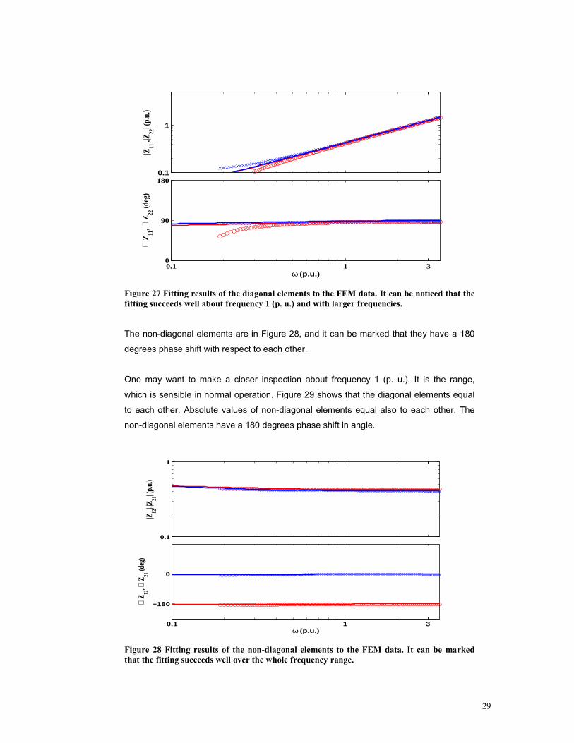
Figure 27 Fitting results of the diagonal elements to the FEM data. It can be noticed that the
fitting succeeds well about frequency 1 (p. u.) and with larger frequencies.
The non-diagonal elements are in Figure 28, and it can be marked that they have a 180
degrees phase shift with respect to each other.
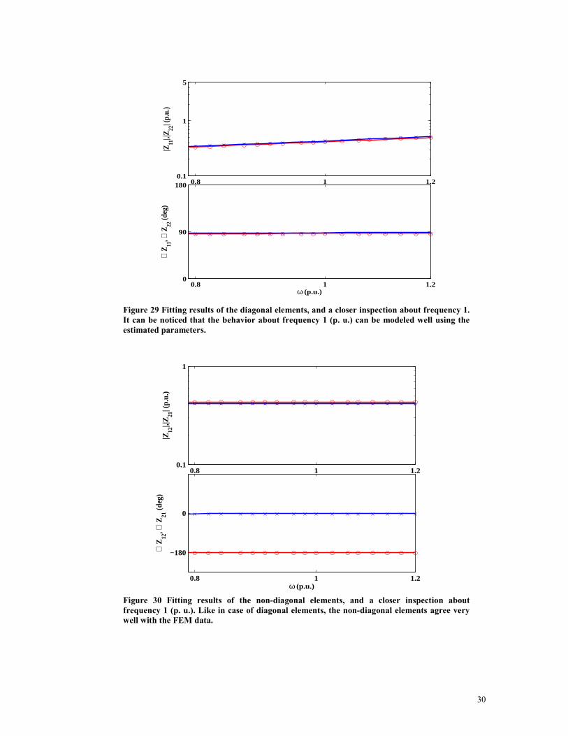
One may want to make a closer inspection about frequency 1 (p. u.). It is the range,
which is sensible in normal operation. Figure 29 shows that the diagonal elements equal
to each other. Absolute values of non-diagonal elements equal also to each other. The
non-diagonal elements have a 180 degrees phase shift in angle.
0.1
1
|Z12
|,|Z 21
| (p.
u.)
0.1 1 3
−180
0
∠ Z 12
, ∠ Z
21 (d
eg)
ω (p.u.)
Figure 28 Fitting results of the non-diagonal elements to the FEM data. It can be marked
that the fitting succeeds well over the whole frequency range.
30
0.8 1 1.20.1
1
5
|Z11
|,|Z 22
| (p.
u.)
0.8 1 1.20
90
180
∠ Z
11, ∠
Z22
(deg
)
ω (p.u.)
Figure 29 Fitting results of the diagonal elements, and a closer inspection about frequency 1.
It can be noticed that the behavior about frequency 1 (p. u.) can be modeled well using the
estimated parameters.
0.8 1 1.20.1
1
|Z12
|,|Z 21
| (p.
u.)
0.8 1 1.2
−180
0
∠ Z
12, ∠
Z21
(deg
)
ω (p.u.)
Figure 30 Fitting results of the non-diagonal elements, and a closer inspection about
frequency 1 (p. u.). Like in case of diagonal elements, the non-diagonal elements agree very
well with the FEM data.
31
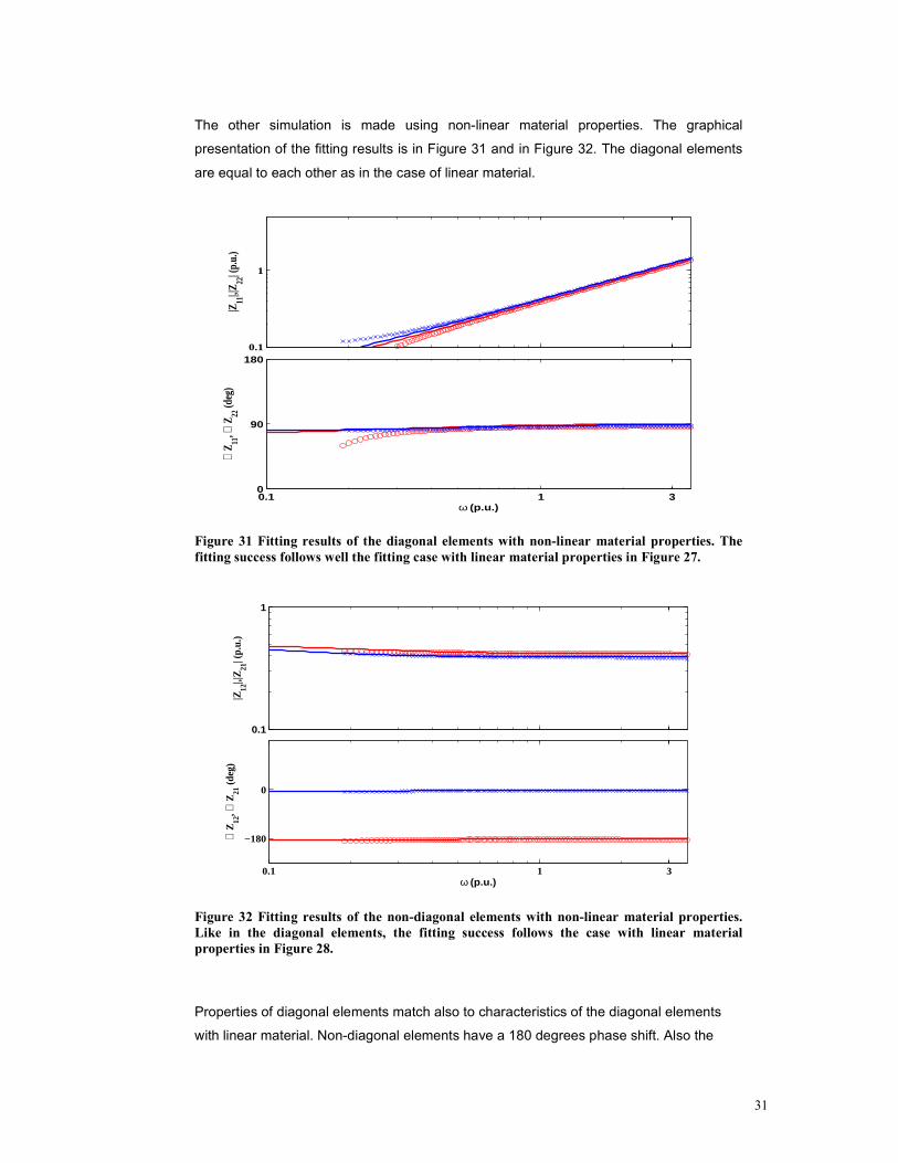
The other simulation is made using non-linear material properties. The graphical
presentation of the fitting results is in Figure 31 and in Figure 32. The diagonal elements
are equal to each other as in the case of linear material.
0.1
1
|Z11
|,|Z 22
| (p.
u.)
0.1 1 30
90
180
∠ Z 11
, ∠ Z
22 (d
eg)
ω (p.u.)
Figure 31 Fitting results of the diagonal elements with non-linear material properties. The
fitting success follows well the fitting case with linear material properties in Figure 27.
0.1
1
|Z12
|,|Z 21
| (p.
u.)
0.1 1 3
−180
0
∠ Z
12, ∠
Z21
(deg
)
ω (p.u.)
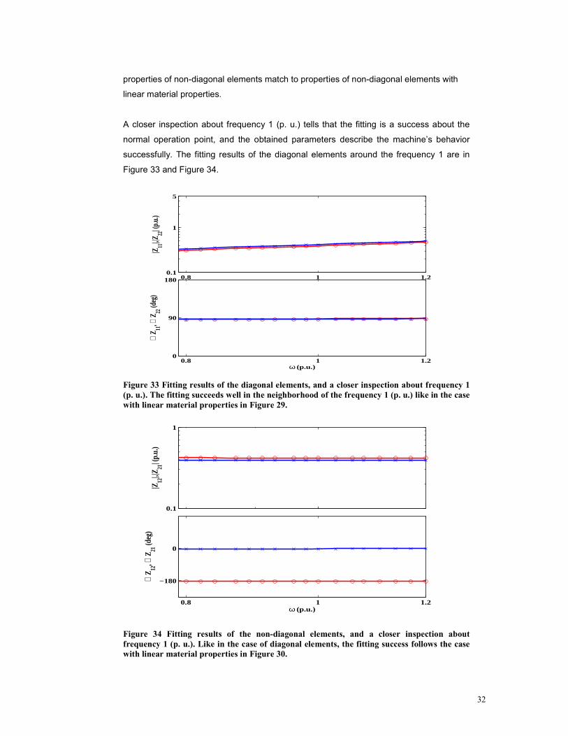
Figure 32 Fitting results of the non-diagonal elements with non-linear material properties.
Like in the diagonal elements, the fitting success follows the case with linear material
properties in Figure 28.
Properties of diagonal elements match also to characteristics of the diagonal elements
with linear material. Non-diagonal elements have a 180 degrees phase shift. Also the
32
properties of non-diagonal elements match to properties of non-diagonal elements with
linear material properties.
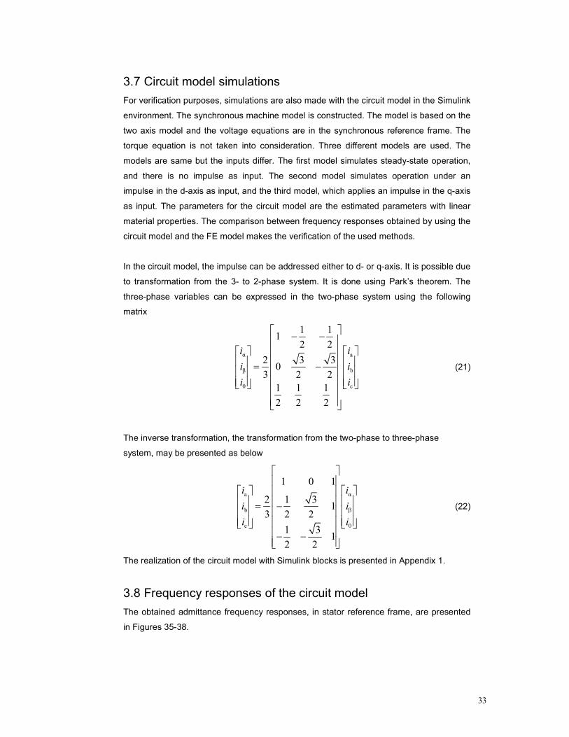
A closer inspection about frequency 1 (p. u.) tells that the fitting is a success about the
normal operation point, and the obtained parameters describe the machine’s behavior
successfully. The fitting results of the diagonal elements around the frequency 1 are in
Figure 33 and Figure 34.
0.8 1 1.20.1
1
5
|Z11
|,|Z22
| (p.
u.)
0.8 1 1.20
90
180
∠ Z 11
, ∠ Z
22 (d
eg)
ω (p.u.)
Figure 33 Fitting results of the diagonal elements, and a closer inspection about frequency 1
(p. u.). The fitting succeeds well in the neighborhood of the frequency 1 (p. u.) like in the case
with linear material properties in Figure 29.
0.1
1
|Z12
|,|Z 21
| (p.
u.)
0.8 1 1.2
−180
0
∠ Z 12
, ∠ Z
21 (d
eg)
ω (p.u.)
Figure 34 Fitting results of the non-diagonal elements, and a closer inspection about
frequency 1 (p. u.). Like in the case of diagonal elements, the fitting success follows the case
with linear material properties in Figure 30.
33
3.7 Circuit model simulations
For verification purposes, simulations are also made with the circuit model in the Simulink
environment. The synchronous machine model is constructed. The model is based on the
two axis model and the voltage equations are in the synchronous reference frame. The
torque equation is not taken into consideration. Three different models are used. The
models are same but the inputs differ. The first model simulates steady-state operation,
and there is no impulse as input. The second model simulates operation under an
impulse in the d-axis as input, and the third model, which applies an impulse in the q-axis
as input. The parameters for the circuit model are the estimated parameters with linear
material properties. The comparison between frequency responses obtained by using the
circuit model and the FE model makes the verification of the used methods.
In the circuit model, the impulse can be addressed either to d- or q-axis. It is possible due
to transformation from the 3- to 2-phase system. It is done using Park’s theorem. The
three-phase variables can be expressed in the two-phase system using the following
matrix
α a
β b
0 c
1 11
2 2
2 3 30
3 2 2
1 1 1
2 2 2
i i
i i
i i
− − = −
(21)
The inverse transformation, the transformation from the two-phase to three-phase
system, may be presented as below
a α
b β
c 0
1 0 1
2 1 31
3 2 2
1 31
2 2
i i
i i
i i
= −
− −
(22)
The realization of the circuit model with Simulink blocks is presented in Appendix 1.
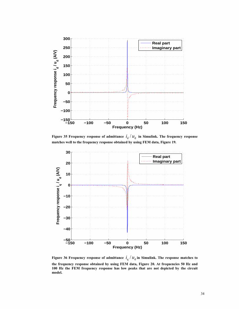
3.8 Frequency responses of the circuit model
The obtained admittance frequency responses, in stator reference frame, are presented
in Figures 35-38.
34
−150 −100 −50 0 50 100 150−150
−100
−50
0
50
100
150
200
250
300
Frequency (Hz)
Freq
uenc
y re
spon
se i
d / u d (A
/V)
Real partImaginary part
Figure 35 Frequency response of admittance d d/i u in Simulink. The frequency response
matches well to the frequency response obtained by using FEM data, Figure 19.
−150 −100 −50 0 50 100 150−50
−40
−30
−20
−10
0
10
20
30
Frequency (Hz)
Freq
uenc
y re
spon
se i
q / u d (A
/V)
Real partImaginary part
Figure 36 Frequency response of admittance q d/i u in Simulink. The response matches to
the frequency response obtained by using FEM data, Figure 20. At frequencies 50 Hz and
100 Hz the FEM frequency response has low peaks that are not depicted by the circuit
model.
35
−150 −100 −50 0 50 100 150−50
−40
−30
−20
−10
0
10
20
30
Frequency (Hz)
Freq
uenc
y re
spon
se i
d / u q (A
/V)
Real partImaginary part
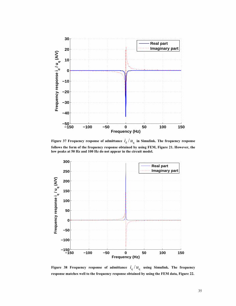
Figure 37 Frequency response of admittance d q/i u in Simulink. The frequency response
follows the form of the frequency response obtained by using FEM, Figure 21. However, the
low peaks at 50 Hz and 100 Hz do not appear in the circuit model.
−150 −100 −50 0 50 100 150−150
−100
−50
0
50
100
150
200
250
300
Frequency (Hz)
Freq
uenc
y re
spon
se i
q / u q (A
/V)
Real partImaginary part
Figure 38 Frequency response of admittance q q/i u using Simulink. The frequency
response matches well to the frequency response obtained by using the FEM data, Figure 22.
36
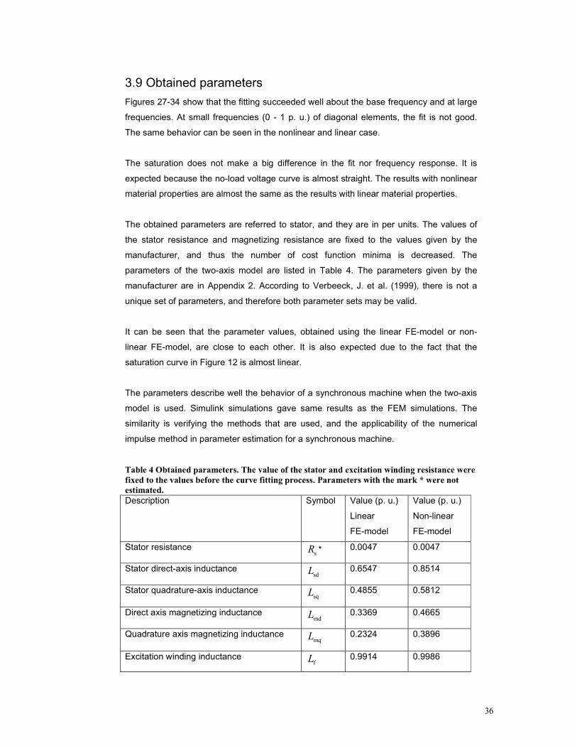
3.9 Obtained parameters
Figures 27-34 show that the fitting succeeded well about the base frequency and at large
frequencies. At small frequencies (0 - 1 p. u.) of diagonal elements, the fit is not good.
The same behavior can be seen in the nonlinear and linear case.
The saturation does not make a big difference in the fit nor frequency response. It is
expected because the no-load voltage curve is almost straight. The results with nonlinear
material properties are almost the same as the results with linear material properties.
The obtained parameters are referred to stator, and they are in per units. The values of
the stator resistance and magnetizing resistance are fixed to the values given by the
manufacturer, and thus the number of cost function minima is decreased. The
parameters of the two-axis model are listed in Table 4. The parameters given by the
manufacturer are in Appendix 2. According to Verbeeck, J. et al. (1999), there is not a
unique set of parameters, and therefore both parameter sets may be valid.
It can be seen that the parameter values, obtained using the linear FE-model or non-
linear FE-model, are close to each other. It is also expected due to the fact that the
saturation curve in Figure 12 is almost linear.
The parameters describe well the behavior of a synchronous machine when the two-axis
model is used. Simulink simulations gave same results as the FEM simulations. The
similarity is verifying the methods that are used, and the applicability of the numerical
impulse method in parameter estimation for a synchronous machine.
Table 4 Obtained parameters. The value of the stator and excitation winding resistance were
fixed to the values before the curve fitting process. Parameters with the mark * were not
estimated.
Description Symbol Value (p. u.)
Linear
FE-model
Value (p. u.)
Non-linear
FE-model
Stator resistance sR * 0.0047 0.0047
Stator direct-axis inductance sdL 0.6547 0.8514
Stator quadrature-axis inductance sqL 0.4855 0.5812
Direct axis magnetizing inductance mdL 0.3369 0.4665
Quadrature axis magnetizing inductance mqL 0.2324 0.3896
Excitation winding inductance fL 0.9914 0.9986
37
Excitation winding resistance fR * 0.0009 0.0009
D-axis damper winding inductance DL 0.8937 0.8973
D-axis damper winding resistance DR 0.1001 0.0403
Q-axis damper winding inductance QL 0.9791 0.9289
Q-axis damper winding resistance QR 0.2075 0.0838
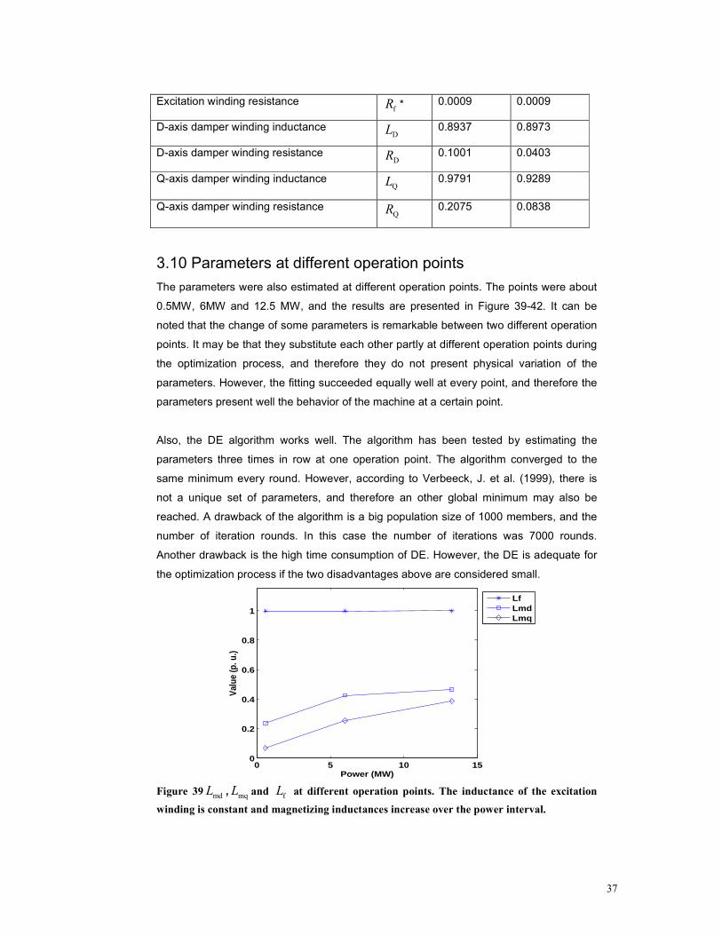
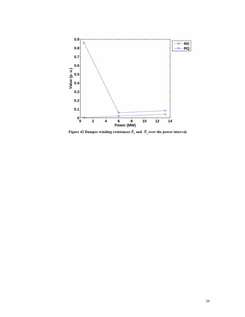
3.10 Parameters at different operation points
The parameters were also estimated at different operation points. The points were about
0.5MW, 6MW and 12.5 MW, and the results are presented in Figure 39-42. It can be
noted that the change of some parameters is remarkable between two different operation
points. It may be that they substitute each other partly at different operation points during
the optimization process, and therefore they do not present physical variation of the
parameters. However, the fitting succeeded equally well at every point, and therefore the
parameters present well the behavior of the machine at a certain point.
Also, the DE algorithm works well. The algorithm has been tested by estimating the
parameters three times in row at one operation point. The algorithm converged to the
same minimum every round. However, according to Verbeeck, J. et al. (1999), there is
not a unique set of parameters, and therefore an other global minimum may also be
reached. A drawback of the algorithm is a big population size of 1000 members, and the
number of iteration rounds. In this case the number of iterations was 7000 rounds.
Another drawback is the high time consumption of DE. However, the DE is adequate for
the optimization process if the two disadvantages above are considered small.
0 5 10 150
0.2
0.4
0.6
0.8
1
Power (MW)
Valu
e (p
. u.)
LfLmdLmq
Figure 39 mdL , mqL and fL at different operation points. The inductance of the excitation
winding is constant and magnetizing inductances increase over the power interval.
38
0 5 10 150.4
0.5
0.6
0.7
0.8
0.9
1
1.1
Power (MW)
Val
ue (
p. u
.)
LsdLsq
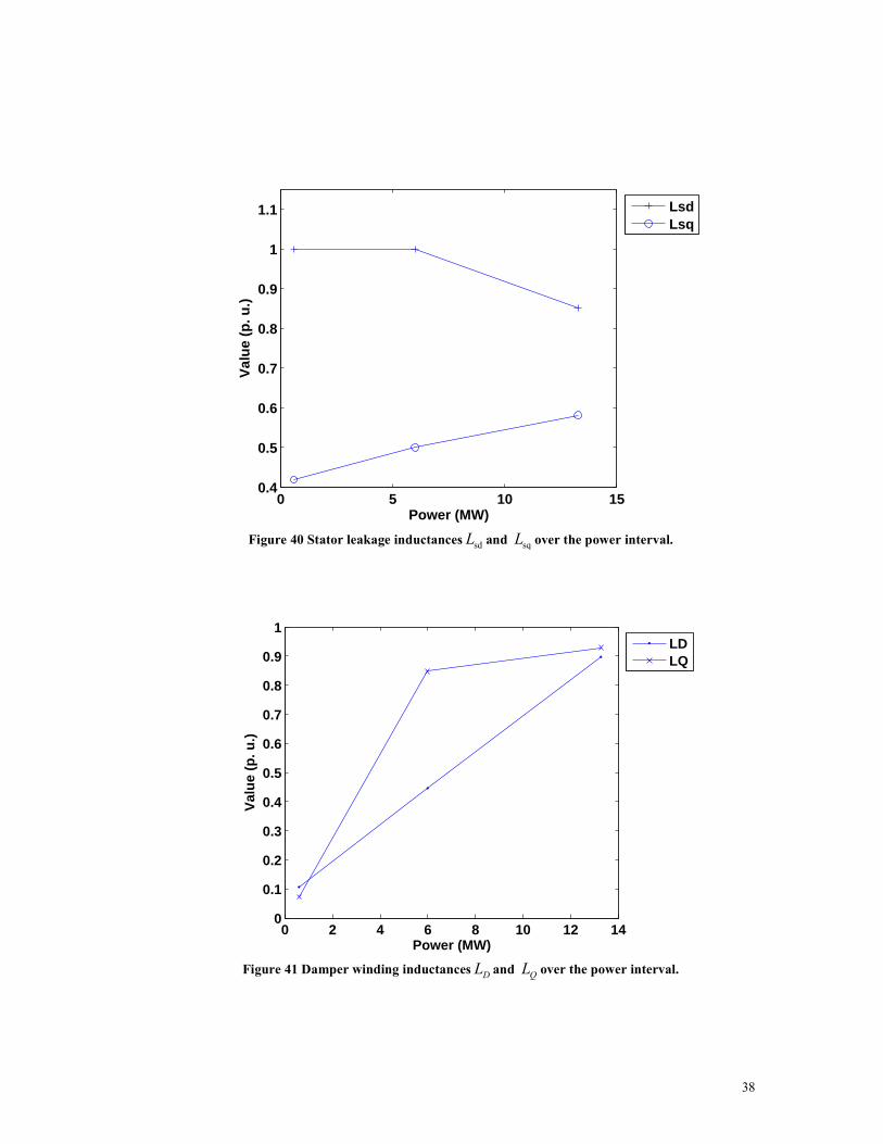
Figure 40 Stator leakage inductances sdL and sqL over the power interval.
0 2 4 6 8 10 12 140
0.1
0.2
0.3
0.4
0.5
0.6
0.7
0.8
0.9
1
Power (MW)
Val
ue (
p. u
.)
LDLQ
Figure 41 Damper winding inductancesDL and
QL over the power interval.
39
0 2 4 6 8 10 12 140
0.1
0.2
0.3
0.4
0.5
0.6
0.7
0.8
0.9
Power (MW)
Val
ue (
p. u
.)
RDRQ
Figure 42 Damper winding resistances RDand R
Qover the power interval.
40
4 Discussion
The two axis model parameters of a synchronous machine have been estimated using
the numerical impulse method. Unlike the standstill frequency response test, the
proposed method is describing the behavior of the machine at other operation points as
well. The parameters are extracted from the data using an evolution algorithm. The
obtained parameters have been verified using circuit simulations in the Simulink-
environment.
Although, the standard two axis model and the estimated parameters describe the
behavior of the machine well, higher order models may be more interesting. An accurate
prediction of machine’s behavior is desirable. Also, the model that takes the mutual
inductance between excitation and damper windings into account may be of interest in
many cases. Research of the applicability of the impulse response method in the cases
above may be reasonable in the future.
The number of time-stepping finite element simulations might be possible to decrease
compare to the arrangement presented in Figure 16. If the behavior of the machine is
considered linear about an operation point, only one time-stepping finite element
simulation might be needed. Based on the results, the linear behavior of the machine is a
reasonable approximation about an operation point. Thus, the time consumption of the
simulation stage could be decreased.
The minimization of the cost function has been made using an evolution algorithm called
Differential Evolution. The algorithm suits well for the minimization. The algorithm did
catch the same minimum every time. The size of the population needs to be high, as well
as, the number of iteration rounds. However, according to Verbeeck, J. et al. (1999),
there are many global minima in the case when there are more than one damper winding
on the axis. Therefore the algorithm may converge also to another global minimum, and
the same values are not obtained.
The minimization can possibly be made using the Newton iteration or another
conventional optimization method also. It may be that, for example, the Newton iteration
needs good initial values so that it converges, but in the case of convergence, the
Newton iteration is fast. In the neighborhood of the solution, the convergence of the
Newton iteration is quadratic. Optimization using an evolution algorithm is time-
consuming, and therefore, the possibility to apply Newton iteration, for instance, in
context of the numerical impulse method is interesting.
41
Good initial values for the iteration may be achieved using the properties of the frequency
response. There is a publication written by Henschel et al. (1999), which covers an idea
obtaining the values of the parameters directly from the frequency response. The idea
may be interesting, and the suitability with the numerical impulse method may be
investigated in the future.
Saturation does not affect much in the investigated machine but a model for saturation
may be of interest in cases where saturation effects are noticeable. The model should be
built and the applicability of the model should be tested in context of the numerical
impulse method.
The parameters have been estimated at different operation points and it can be noticed
that the variation in parameters may not be the physical variation of the parameters. They
may substitute each other partly at different points. However, they describe well the
behavior of the machine at operation points. In the future, it may be reasonable to try to
change the optimization process so that the variations of the parameters describe the
physical variations of the parameters. Also, the fit at low frequencies is not good. This
issue is also of interest in the future.
Measurements are needed in order to verify the obtained parameters. To obtain the
frequency responses under study, the harmonic excitation experiments may be needed.
However, the frequency responses obtained using the Simulink circuit model with
estimated parameters match well with FEM simulations.
The studied machine is a salient pole synchronous machine with an excitation winding.
However, in the future, permanent magnet synchronous machines are getting more and
more common. Therefore, the applicability of the numerical impulse method is of interest
in context of permanent magnet synchronous machines.
42
5 Conclusion
The suitability of the numerical impulse method for the synchronous machine parameter
estimation has been studied. The two-axis model parameters have been estimated using
FEM data, and the results are reasonable. The parameters are valid about the operation
point selected. The parameters have been estimated using linear and nonlinear material
FE-models. The estimated parameters are verified using circuit simulations in the
Simulink environment. The results obtained from the circuit and FEM simulations match
well with each other.
Linearized equations may be used for describing the behavior about an operation point. A
linearization method for the two-axis model equations taking advantage of the Taylor’s
expansion is presented. From the linearized equations a transfer function between the
current and voltage will be formulated. A formulation exploiting results in control theory
has been presented. Lastly, the transfer function is fitted into the numerical transfer
function produced by FEM simulations, and thus the parameters can be achieved.
The fitting is made using a Differential Evolution algorithm. It has been noticed that it is
easy to use and an effective tool for the fitting process. The algorithm does converge to
the minimum round after round, but the size of population members is high, as well as,
the number of iteration rounds. In case of more than one damper winding, there are n
factorial (n!) global minima. A drawback in the Differential Evolution algorithm is the time
consumption.
The obtained values of the parameters, using the linear and non-linear FE-model are
quite close to each other. The result is expected because the magnetizing curve is almost
linear. It also seems that the parameters describe well the desired input/output behavior
based on the experiments made using the circuit model in the Simulink environment.
An MIMO-system model for a synchronous machine is presented. In that representation,
the outputs and inputs are the d- and q-axis currents and voltages, and the transfer
function is a 2x2 admittance or impedance matrix. In the optimizing process, the size of
the matrix is measured by the Frobenius norm.
The permitted impulse size in the circuit model has been studied using Lyapunov stability
analysis. It can be interpreted that there is only one steady state, and the system is stable
regardless of the impulse size.
43
The effect of the amplitude of the impulse in the FEM-simulations using the nonlinear
material FE-model has been studied using three different impulse amplitudes, 1%, 10%
and 20% of the average RMS-value of the line voltages. It can be noticed that the
difference in frequency responses is very small, and the effect of the impulse amplitude is
small with the studied amplitudes. Therefore the linearization about an operation point is
reasonable.
The numerical impulse method is suitable for the parameter estimation of synchronous
machines. The great advantage of the impulse method is that the obtained parameters
describe the real operation point of the machine. Also the saturation is considered.
Additionally, the proposed method is not stressful on experimental measurements for the
machine because high current peaks can be avoided, unlike in the sudden short circuit
test.
44
6 References
Bastos, J. P. A. & Sadowski N. 2003, Electromagnetic Modelin by Finite Element
Methods, Marcel Dekker, Inc., New York
Bortoni, E. C. & Jardini, J. A. 2004, A Standstill Frequency Response Method for Large
Salient Pole Synchronous Machines, IEEE Transactions on Energy Conversion, Vol. 19,
No. 4, December 2004, pp. 687-691
Burakov, A. & Arkkio, A. 2006, Low-order parametric force model for a salient-pole
synchronous machine with eccentric rotor, Electrical Engineering 89: 127-136
Electric Machinery Committee of the IEEE Power Engineering Society 1995, IEEE Guide:
Test Procedures for Synchronous Machines
Glad, T. & Ljung, L. 2000, Control Theory: Multivariable and Nonlinear Methods, Taylor &
Francis, Great Britain
Henschel, S. & Dommel, H. W. 1999, Noniterative Synchronous Machine Parameter
Identification from Frequency Response Tests, IEEE Transactions on Power Systems,
Vol. 14, No. 2, May 1999, pp. 553-560
Holopainen, T. 2004, Electromechanical interaction in rotordynamics of cage induction
motors, VTT Publications 543. Online: http://lib.tkk.fi/Diss/2004/isbn9513864057/
Keyhani, A. & Tsai, H. 1994, Identification of High-Order Synchronous Generator Models
from SSFR Test Data, IEEE Transactions on Energy Conversion, Vol. 9, No. 3,
September 1994, pp. 593-603
Krause, P. C., Wasynczuk, O. & Sudhoff, S. D. 2002, Analysis of Electric Machinery and
Drive Systems, Wiley-Interscience, USA
Luomi, J. 1998, Transient Phenomena in Electrical Machines, lecture notes at Chalmers
University of Technology, Göteborg
Luomi, J., Niiranen, J. & Niemenmaa, A. 2005, Sähkömekaniikka ja sähkökäytöt osa 2 (in
Finnish), Helsinki University of Technology, Espoo
45
Müller, G. 1985, Elektrische Maschinen: Betriebsverhalten rotierender elektrischer
Maschinen, VEB Verlag Technik Berlin
Price, K. V., Storn R. M. & Lampinen J. A. 2005, Differential Evolution A Practical
Approach to Global Optimization, Springer, Heidelberg
Repo, A. -K. & Arkkio, A. 2006a, Parameter estimation of induction machines using the
numerical impulse method, SPEEDAM 2006 23-26 May, Taormina Italy, International
Symposium on Power Electronics, Electrical Drives, Automation and Motion, 2006, pp.
943-948
Repo, A. -K. & Arkkio, A. 2006b, Numerical impulse response test to estimate circuit-
model parameters for induction machines, IEE Proceedings-Electrical Power
Applications, Vol. 153, No.6, November 2006, pp. 883-890
Repo, A.-K. & Arkkio, A. 2007, Numerical impulse response test to identify parametric
models for closed-slot deep-bar induction motors, IET Electrical Power Applications, Vol.
1, No. 3, May 2007, pp. 307-315
Struble, R. A. 1962, Nonlinear Differential Equations, McGraw-Hill Book Company
Tenhunen, A. 2003, Electeromagnetic forces acting between the stator and eccentric
cage rotor, Doctoral Thesis, Helsinki University of Technology, Laboratory of
Electromechanics, Report 69, Espoo 2003. Online:
http://lib.tkk.fi/Diss/2003/isbn9512266830/
Verbeeck, J., Pintelon, R. & Guillaume, P. 1999, Determination of Synchronous Machine
Parameters Using Network Synthesis Techniques, IEEE Transactions on Energy
Conversion, Vol. 14, No. 3, September 1999, pp. 310-314
Wamkeue, R., Kamwa, I. & Chacha M. 2003, Line-to-Line Short-Circuit-Based Finite-
Element Performance and Parameter Predictions of Large Hydrogenerators, IEEE
Transactions on Energy Conversion, Vol. 18, No. 3, September 2003, pp. 370-378
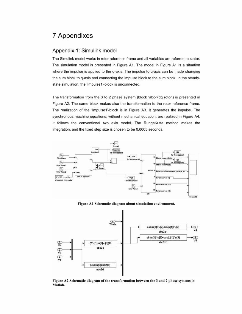
7 Appendixes
Appendix 1: Simulink model
The Simulink model works in rotor reference frame and all variables are referred to stator.
The simulation model is presented in Figure A1. The model in Figure A1 is a situation
where the impulse is applied to the d-axis. The impulse to q-axis can be made changing
the sum block to q-axis and connecting the impulse block to the sum block. In the steady-
state simulation, the ‘Impulse1’-block is unconnected.
The transformation from the 3 to 2 phase system (block ‘abc->dq rotor’) is presented in
Figure A2. The same block makes also the transformation to the rotor reference frame.
The realization of the ‘Impulse1’-block is in Figure A3. It generates the impulse. The
synchronous machine equations, without mechanical equation, are realized in Figure A4.
It follows the conventional two axis model. The RungeKutta method makes the
integration, and the fixed step size is chosen to be 0.0005 seconds.
Figure A1 Schematic diagram about simulation environment.
Figure A2 Schematic diagram of the transformation between the 3 and 2 phase systems in
Matlab.
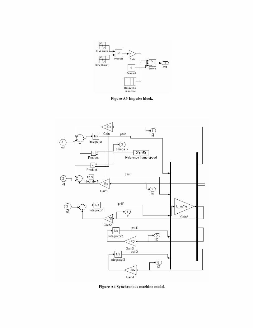
Figure A3 Impulse block.
Figure A4 Synchronous machine model.
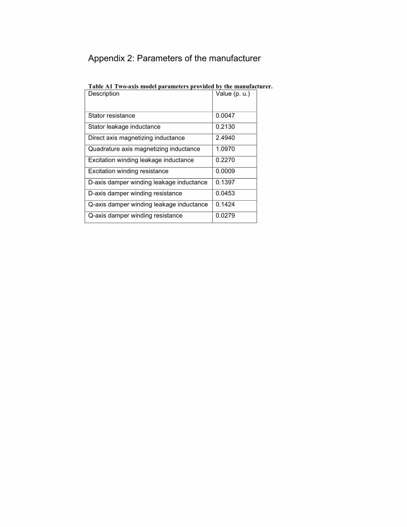
Appendix 2: Parameters of the manufacturer
Table A1 Two-axis model parameters provided by the manufacturer.
Description Value (p. u.)
Stator resistance 0.0047
Stator leakage inductance 0.2130
Direct axis magnetizing inductance 2.4940
Quadrature axis magnetizing inductance 1.0970
Excitation winding leakage inductance 0.2270
Excitation winding resistance 0.0009
D-axis damper winding leakage inductance 0.1397
D-axis damper winding resistance 0.0453
Q-axis damper winding leakage inductance 0.1424
Q-axis damper winding resistance 0.0279