Embed Size (px)
Citation preview

PARAMETER ESTIMATION FOR LINEARDYNAMICAL SYSTEMS WITH APPLICATIONS TO
EXPERIMENTAL MODAL ANALYSIS
A Thesis Submitted tothe Graduate School of Engineering and Sciences of
Izmir Institute of Technologyin Partial Fulfillment of the Requirements for the Degree of
MASTER OF SCIENCE
in Electrical and Electronics Engineering
byIlker Tanyer
August 2008IZMIR

We approve the thesis of Ilker Tanyer
Date of Signature
. . . . . . . . . . . . . . . . . . . . . . . . . . . . . . . . . . . . . 15 July 2008Assist. Prof. Dr. Serdar OZENSupervisorDepartment of Electrical and Electronics EngineeringIzmir Institute of Technology
. . . . . . . . . . . . . . . . . . . . . . . . . . . . . . . . . . . . . 15 July 2008Assist. Prof. Dr. Cemalettin DONMEZDepartment of Civil EngineeringIzmir Institute of Technology
. . . . . . . . . . . . . . . . . . . . . . . . . . . . . . . . . . . . . 15 July 2008Assoc. Prof. Dr. Bilge KARACALIDepartment of Electrical and Electronics EngineeringIzmir Institute of Technology
. . . . . . . . . . . . . . . . . . . . . . . . . . . . . . . . . . . . . 15 July 2008Assist. Prof. Dr. Mustafa Aziz ALTINKAYADepartment of Electrical and Electronics EngineeringIzmir Institute of Technology
. . . . . . . . . . . . . . . . . . . . . . . . . . . . . . . . . . . . . 15 July 2008Assoc. Prof. Dr. Serhan OZDEMIRDepartment of Electrical and Electronics EngineeringIzmir Institute of Technology
. . . . . . . . . . . . . . . . . . . . . . . . . . . . . . . . . . . . . 15 July 2008
Prof. Dr. F.Acar SAVACIHead of DepartmentDepartment of Electrical and Electronics EngineeringIzmir Institute of Technology
. . . . . . . . . . . . . . . . . . . . . . . . . .Prof. Dr. Hasan BOKE
Head of the Graduate School

ACKNOWLEDGEMENTS
First of all, i would like to thank my supervisors, Assist. Prof. Dr. Serdar OZEN
and Assist. Prof. Dr. Cemalettin DONMEZ for spending their time to help me in this
project.
I thank Assist. Prof. Dr. Cemalettin DONMEZ and R.A. Eyyub KARAKAN
for experimental measurements, giving knowledge about vibration theory and analytical
solutions.
Also I would like to thank Assist. Prof. Dr. Mustafa Aziz ALTINKAYA for
helping me about pre-processing and simulations of ERA.
In addition, I would like to thank Assist. Prof. Dr. Serdar OZEN, Assist. Prof.
Dr. Cemalettin DONMEZ, Assoc. Prof. Dr. Bilge KARACALI, Assist. Prof.Dr. Mustafa
Aziz ALTINKAYA and Assoc.Prof.Dr. Serhan OZDEMIR for giving me corrections and
suggestions which helped me a lot in revising the thesis.
This project is funded by TUBITAK with project number 104I107, therefore i
would like to thank TUBITAK for their support.
Finally I would like to thank my family, Ilkay, Koksal-Devlet TANYER for their
help and support. This project is also dedicated to my family as my other projects.

ABSTRACT
PARAMETER ESTIMATION FOR LINEAR DYNAMICAL SYSTEMS
WITH APPLICATIONS TO EXPERIMENTAL MODAL ANALYSIS
In this study the fundamentals of structural dynamics and system identification
have been studied. Then some fundamental parameter estimation algorithms in the liter-
ature are provided. These algorithms will be applied to an experimental and an artificial
system to extract their structural properties. Consequently, the main objective of this study
is constructing the mathematical model of a structure by using only the measurement data.
To process measurement data, three fundamental modal analysis algorithms are
examined. Least-Squares Complex Exponential(LSCE), Eigensystem Realization Algo-
rithm(ERA) and Polyreference Frequency Domain(PFD) algorithms are implemented in
MATLAB environment. We applied these algorithms to artificial and experimental data,
then we compared the performance of these algorithms. State estimation for linear dy-
namical systems have also been studied, and details of the Kalman filter as a state esti-
mator are provided. Kalman filter as a state estimator has been integrated with the ERA
algorithm and the performance of the Kalman-ERA is provided.
iv

OZET
DOGRUSAL DINAMIK SISTEMLER ICIN DEGISKEN KESTIRIMI
VE DENEYSEL MODAL ANALIZ UYGULAMALARI
Bu calısmada yapı dinamigi ve sistem tanılamanın temelleri gozden gecirilecektir.
Ardından literaturdeki bazı temel parametre kestirim algoritmaları anlatılacaktır. Bu al-
goritmalar yapay ve deneysel sistemlere uygulanacak ve bu sistemlerin yapısal ozellikleri
bulunmaya calısılacaktır. Kısaca calısmadaki asıl amac sadece yapıdan alınan olcumleri
kullanarak yapının matematiksel modelini olusturmaktır.
Olcum verilerini isleyebilmek icin uc temel Modal Analiz algoritması
incelenmistir. En Kucuk Kareler Karmasık Ustel Metodu, Ozsistem Gerceklestirme
Algoritması ve Coklu Referans Frekans Bolgesi algoritmaları MATLAB ortamında
gerceklenmistir. Bu algoritmalar yapay ve deneysel verilere uygulanmıs ve algoritmaların
performansları karsılastırılmıstır. Ayrıca Kalman suzgeci bir durum kestiricisi olarak kul-
lanılarak dogrusal dinamik sistemler icin durum kestirimi islemi incelenmis ve daha dogru
bir parametre kestirimi yapmak adına Kalman suzgeci Ozsistem Gerceklestirme Algorit-
ması ile birlestirilmistir.
v

TABLE OF CONTENTS
LIST OF FIGURES . . . . . . . . . . . . . . . . . . . . . . . . . . . . . . . . viii
LIST OF ABBREVIATIONS . . . . . . . . . . . . . . . . . . . . . . . . . . . x
CHAPTER 1 . INTRODUCTION . . . . . . . . . . . . . . . . . . . . . . . . . 1
1.1. Overview . . . . . . . . . . . . . . . . . . . . . . . . . . . . 1
1.2. Background . . . . . . . . . . . . . . . . . . . . . . . . . . . 5
1.2.1. Analysis of Single Degree of Freedom Systems . . . . . . 8
1.2.2. Analysis of Multi Degree of Freedom Systems . . . . . . 16
1.3. Main Goal . . . . . . . . . . . . . . . . . . . . . . . . . . . . 19
CHAPTER 2 . SIMPLE ESTIMATION METHODS . . . . . . . . . . . . . . . 21
2.1. Frequency Domain Estimation . . . . . . . . . . . . . . . . . 21
2.2. Time Domain Estimation . . . . . . . . . . . . . . . . . . . . 24
CHAPTER 3 . PRE-PROCESSING TECHNIQUES . . . . . . . . . . . . . . . 28
3.1. Frequency Domain Division Method . . . . . . . . . . . . . . 28
3.2. Time Domain IRF Estimation Method . . . . . . . . . . . . . 30
3.3. Comparison of IRF Estimation Methods . . . . . . . . . . . . 33
CHAPTER 4 . POLYREFERENCE FREQUENCY DOMAIN METHOD . . . . 36
4.1. State Space Representation . . . . . . . . . . . . . . . . . . . 36
4.2. Frequency Domain Algorithm . . . . . . . . . . . . . . . . . 39
CHAPTER 5 . LEAST SQUARES COMPLEX EXPONENTIAL METHOD . . 48
CHAPTER 6 . EIGENSYSTEM REALIZATION ALGORITHM . . . . . . . . 53
CHAPTER 7 . STATE ESTIMATION FOR DYNAMICAL SYSTEMS . . . . . 59
CHAPTER 8 . COMPARISON OF SIMULATION RESULTS . . . . . . . . . . 68
CHAPTER 9 . CONCLUSION AND FUTURE WORK . . . . . . . . . . . . . 70
vi

9.1. Conclusion . . . . . . . . . . . . . . . . . . . . . . . . . . . 70
9.2. Future Work . . . . . . . . . . . . . . . . . . . . . . . . . . . 71
REFERENCES . . . . . . . . . . . . . . . . . . . . . . . . . . . . . . . . . . . 75
APPENDICES
APPENDIX A. MATLAB SCRIPTS . . . . . . . . . . . . . . . . . . . . . . . 76
vii

LIST OF FIGURES
Figure Page
Figure 1.1. Transamerica Pyramid Building in San Francisco . . . . . . . . . . 1
Figure 1.2. Experimental Setup . . . . . . . . . . . . . . . . . . . . . . . . . . 2
Figure 1.3. Schematic Diagram for a 4 story frame . . . . . . . . . . . . . . . . 3
Figure 1.4. A Vibratory System . . . . . . . . . . . . . . . . . . . . . . . . . . 6
Figure 1.5. Mechanical Elements . . . . . . . . . . . . . . . . . . . . . . . . . 6
Figure 1.6. Mass-Spring System . . . . . . . . . . . . . . . . . . . . . . . . . . 9
Figure 1.7. Free Vibration of SDOF Undamped System . . . . . . . . . . . . . 11
Figure 1.8. Mass-Spring-Damper System . . . . . . . . . . . . . . . . . . . . . 12
Figure 1.9. Free Vibration of SDOF Damped System . . . . . . . . . . . . . . . 13
Figure 1.10. Comparison of Undamped System and Underdamped System . . . . 14
Figure 1.11. Mass-Spring-Damper System with Input . . . . . . . . . . . . . . . 15
Figure 1.12. 2-DOF System . . . . . . . . . . . . . . . . . . . . . . . . . . . . . 16
Figure 2.1. Real part of the FRF . . . . . . . . . . . . . . . . . . . . . . . . . . 23
Figure 2.2. Imaginary part of the FRF . . . . . . . . . . . . . . . . . . . . . . . 24
Figure 2.3. Magnitude of the FRF . . . . . . . . . . . . . . . . . . . . . . . . . 25
Figure 2.4. Phase of the FRF . . . . . . . . . . . . . . . . . . . . . . . . . . . 26
Figure 2.5. Impulse Response Function . . . . . . . . . . . . . . . . . . . . . . 27
Figure 3.1. Noise Estimation from Input Signal . . . . . . . . . . . . . . . . . . 28
Figure 3.2. Pre-processing . . . . . . . . . . . . . . . . . . . . . . . . . . . . . 30
Figure 3.3. Comparison of h and h . . . . . . . . . . . . . . . . . . . . . . . . 34
Figure 3.4. Error Graph for h and h . . . . . . . . . . . . . . . . . . . . . . . . 34
Figure 3.5. Comparison of h and h . . . . . . . . . . . . . . . . . . . . . . . . 35
Figure 3.6. Error Graph for h and h . . . . . . . . . . . . . . . . . . . . . . . . 35
Figure 4.1. 2-DOF System . . . . . . . . . . . . . . . . . . . . . . . . . . . . . 38
Figure 4.2. Magnitude of the FRF’s of 2-DOF System . . . . . . . . . . . . . . 45
Figure 4.3. Phase of the FRF’s of 2-DOF System . . . . . . . . . . . . . . . . . 46
Figure 5.1. IRF’s of 2-DOF System . . . . . . . . . . . . . . . . . . . . . . . . 51
Figure 7.1. Usage of ERA and Kalman Filter . . . . . . . . . . . . . . . . . . . 59
viii
Figure 7.2. State Estimation and Error with SNR=0dB . . . . . . . . . . . . . . 61
Figure 7.3. State Estimation and Error with SNR=20dB . . . . . . . . . . . . . 62
Figure 7.4. State Estimation and Error with SNR=40dB . . . . . . . . . . . . . 63
Figure 7.5. Chi-square PDF . . . . . . . . . . . . . . . . . . . . . . . . . . . . 64
Figure 7.6. Tabulated values for Chi-Square PDF . . . . . . . . . . . . . . . . . 64
Figure 7.7. NEES with probability Q=0.05 . . . . . . . . . . . . . . . . . . . . 65
Figure 7.8. NEES with probability Q=0.02 . . . . . . . . . . . . . . . . . . . . 66
Figure 7.9. NEES with probability Q=0.01 . . . . . . . . . . . . . . . . . . . . 66
Figure 9.1. The process of SHM . . . . . . . . . . . . . . . . . . . . . . . . . . 70
Figure 9.2. Usage of ERA, Kalman Filter and EM Algorithm . . . . . . . . . . 72
ix
LIST OF ABBREVIATIONS
FRF Frequency response function
IRF Impulse response function
LTI Linear time invariant
EM Expectation-maximization
FFT Fast Fourier transform
LSCE Least squares complex exponential
PFD Polyreference frequency domain
SDOF Single degree of freedom
MDOF Multi degree of freedom
MIMO Multiple-input multiple-output
ML Maximum-likelihood
MMSE Minimum mean squared error
ERA Eigensystem realization algorithm
MLE Maximum likelihood estimation
SNR Signal to noise ratio
x
CHAPTER 1
INTRODUCTION
1.1. Overview
Mechanical , aeronautical or civil structures need to be lighter, stronger and more
flexible because of the demands of safety and reliability. Furthermore predicting the re-
sponse of a structure to an excitation is so critical. Because of these facts, vibration
analysis of structures become a popular subject for engineers. Making experiments on a
structure, constructing a mathematical model, controlling the structure or designing strong
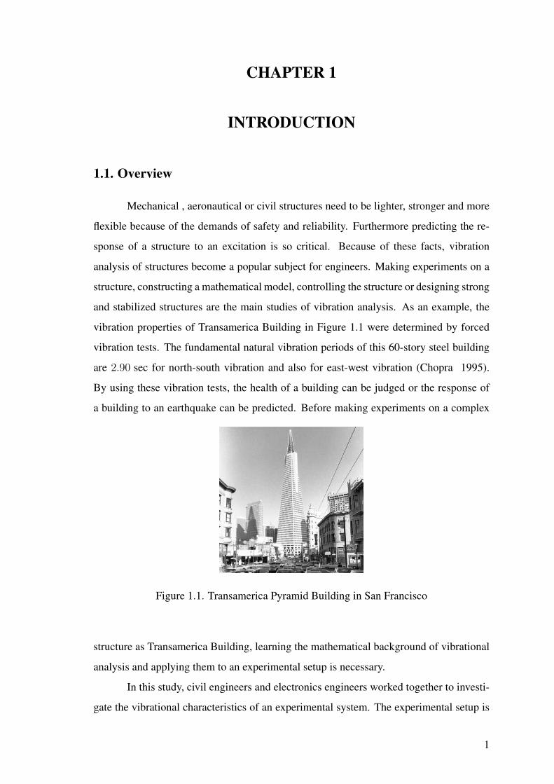
and stabilized structures are the main studies of vibration analysis. As an example, the
vibration properties of Transamerica Building in Figure 1.1 were determined by forced
vibration tests. The fundamental natural vibration periods of this 60-story steel building
are 2.90 sec for north-south vibration and also for east-west vibration (Chopra 1995).
By using these vibration tests, the health of a building can be judged or the response of
a building to an earthquake can be predicted. Before making experiments on a complex
Figure 1.1. Transamerica Pyramid Building in San Francisco
structure as Transamerica Building, learning the mathematical background of vibrational
analysis and applying them to an experimental setup is necessary.
In this study, civil engineers and electronics engineers worked together to investi-
gate the vibrational characteristics of an experimental system. The experimental setup is
1
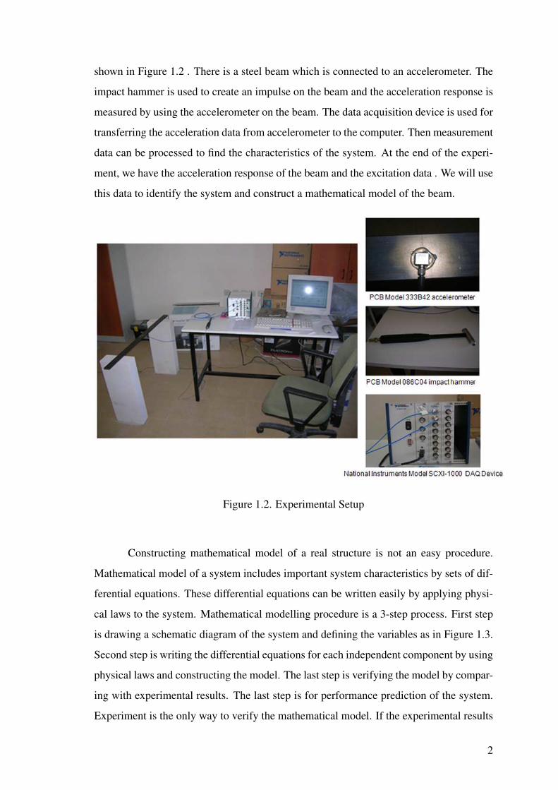
shown in Figure 1.2 . There is a steel beam which is connected to an accelerometer. The
impact hammer is used to create an impulse on the beam and the acceleration response is
measured by using the accelerometer on the beam. The data acquisition device is used for
transferring the acceleration data from accelerometer to the computer. Then measurement
data can be processed to find the characteristics of the system. At the end of the experi-
ment, we have the acceleration response of the beam and the excitation data . We will use
this data to identify the system and construct a mathematical model of the beam.
Figure 1.2. Experimental Setup
Constructing mathematical model of a real structure is not an easy procedure.
Mathematical model of a system includes important system characteristics by sets of dif-
ferential equations. These differential equations can be written easily by applying physi-
cal laws to the system. Mathematical modelling procedure is a 3-step process. First step
is drawing a schematic diagram of the system and defining the variables as in Figure 1.3.
Second step is writing the differential equations for each independent component by using
physical laws and constructing the model. The last step is verifying the model by compar-
ing with experimental results. The last step is for performance prediction of the system.
Experiment is the only way to verify the mathematical model. If the experimental results
2

are different from the prediction, then a modification must be done for the mathematical
model. The process must be repeated until a satisfactory agreement is obtained between
experimental results and prediction.
Figure 1.3. Schematic Diagram for a 4 story frame
Mathematical modelling of dynamical systems and analyzing the dynamical be-
havior of the structures are the subjects of System Dynamics. A system is called dynamical
if its present output depends on past input. If the system’s current output depends only
on the current input, system is called as static. As said before, dynamical systems can
be modelled by differential equations. Classifying differential equations is important for
the classification of the system. According to this classification, the analysis for mod-
elling can be changed. For example if a system has nonlinear differential equations, its
mathematical model will be a nonlinear model and nonlinear analysis must be done for
this system. Mathematically linearity means that the relationship between the input and
the output of the system satisfies the superposition property. According to superposition
property, if the input to the system is the sum of two component signals as
x(t) = ax1(t) + bx2(t) , (1.1)
then the output of the system will be,
y(t) = ay1(t) + by2(t) , (1.2)
where yk(t) for k = 1, 2, are the output signals resulting from the input signals xk(t) for
k = 1, 2, and the coefficients a, b are complex valued scalars.
3
Time invariance is another important system property for dynamical system analysis.
Time invariance means that if the input is affected by a time delay, the output should
be affected by the same time delay. Consider a linear system with impulse response h(t)
where the input-output relationship is given by
y(t) = x(t) ∗ h(t) , (1.3)
where x(t) is the input, y(t) is the output and ∗ is the convolution operator. If a time shift
in the input signal results in an identical time shift in the output signal, as
y(t− t0) = x(t− t0) ∗ h(t) , (1.4)
then h(t) is said to be a linear time-invariant system. If a system satisfies both the linear-
ity and the time invariance properties, this system is called Linear Time Invariant (LTI)
system.
In this study we will deal with the mathematical models of LTI dynamical systems
and we will try to find the characteristics of the system by using System Identification,
Structural Dynamics and Modal Analysis concepts.
System identification is the process of building dynamical models from measured
data by using several mathematical tools and algorithms. In this study, some system iden-
tification techniques will be investigated and these techniques will be verified by MAT-
LAB simulations.
Structural dynamics is the analytical study of the structures which covers the be-
havior of structures when subjected to dynamical loading. Buildings, bridges, satellites,
aircrafts, vehicles can be considered as examples of structures. Dynamical loading can be
wind, wave, earthquake, blasts. Dynamical loading means that the load on the structure
changes with time.
Since the problem of mathematical modelling is so complex, engineers generally
use Finite Element Analysis as a design tool to solve this complexity. Finite element
analysis is a computer modelling approach based on numerical analysis. Modal analysis
is an important part of dynamical finite element analysis and it is a powerful tool for
civil engineers. The main objective of modal analysis can be defined as determining,
improving and optimizing the dynamical characteristics of structures by utilizing modal
analysis and system identification procedures. Modal analysis is a 3-step process. First the
dynamical properties of systems are investigated under vibrational excitation. Then the
4
dynamical characteristics of the system are determined in the form of natural frequencies
and damping ratios. Consequently, these modal parameters can be used to formulate a
mathematical model.
Modal analysis is based upon the fact that the vibration response of a LTI dy-
namical system can be expressed as the linear combination of a set of harmonic motions
called the natural modes of vibration. Actually it is a complicated waveform which can
be represented as a combination of sine and cosine waves. Natural modes of vibration are
special characteristics to dynamical systems and they can be determined by its physical
properties where the physical properties are mass, stiffness, and damping. Natural modes
can be described in terms of natural frequency, modal damping factor and mode shape.
These are also called modal parameters.
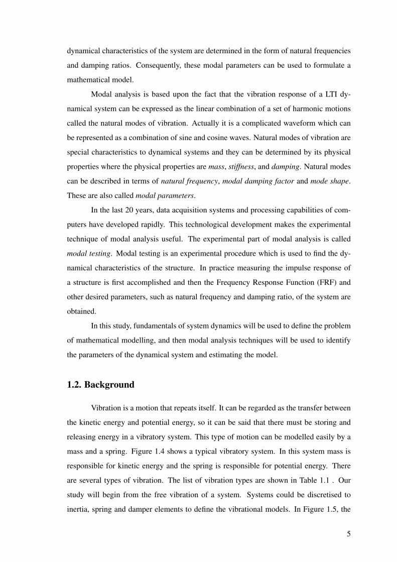
In the last 20 years, data acquisition systems and processing capabilities of com-
puters have developed rapidly. This technological development makes the experimental
technique of modal analysis useful. The experimental part of modal analysis is called
modal testing. Modal testing is an experimental procedure which is used to find the dy-
namical characteristics of the structure. In practice measuring the impulse response of
a structure is first accomplished and then the Frequency Response Function (FRF) and
other desired parameters, such as natural frequency and damping ratio, of the system are
obtained.
In this study, fundamentals of system dynamics will be used to define the problem
of mathematical modelling, and then modal analysis techniques will be used to identify
the parameters of the dynamical system and estimating the model.
1.2. Background
Vibration is a motion that repeats itself. It can be regarded as the transfer between
the kinetic energy and potential energy, so it can be said that there must be storing and
releasing energy in a vibratory system. This type of motion can be modelled easily by a
mass and a spring. Figure 1.4 shows a typical vibratory system. In this system mass is
responsible for kinetic energy and the spring is responsible for potential energy. There
are several types of vibration. The list of vibration types are shown in Table 1.1 . Our
study will begin from the free vibration of a system. Systems could be discretised to
inertia, spring and damper elements to define the vibrational models. In Figure 1.5, the
5

Figure 1.4. A Vibratory System
Table 1.1. Vibration Types
Reference Terms Vibration Type Description
External Excitation Free Vibration Vibration induced by initial input(s) only.
Forced Vibration Vibration subjected to one or more continuous external inputs.
Presence of Damping Undamped Vibration Vibration with no energy loss or dissipation.
Damped Vibration Vibration with energy loss.
Linearity of Vibration Linear Vibration Vibration for which superposition principle holds.
Nonlinear Vibration Vibration that violates superposition principle.
Predictability Deterministic Vibration The value of vibration is known at any given time.
Random Vibration Only the statistical properties of vibration are known.
basic mechanical elements and their force equations are shown. In these force equations
x represents the displacement, dots on the top of variable x represents derivatives with
respect to time; therefore x and x becomes the velocity and acceleration. After defining
the system by using these mechanical elements, mathematical model of the system in
Figure 1.4 can be developed by applying physical laws to the system. In vibrational
Figure 1.5. Mechanical Elements
systems, inertia elements are the masses. Mass is the property of a body that gives inertia
to the body, whereas the inertia is commonly known as the resistance to starting motion
6
and resistance arriving to a full stop while in motion. Newton’s second law, known as law
of acceleration, is used to define the equations of motion of the masses. Newton’s second
law says that (Cohen and Whitman 1999):
Law 1.1 The rate of change of momentum of a body is proportional to the resultant force
acting on the body and is in the same direction.
Mathematical representation of this law is
F = ma , (1.5)
where F is the force, m is the mass and a is the acceleration.
A spring element is a flexible elastic object which is used to store mechanical energy. It
can be deformed by an external force such that the deformation is directly proportional to
the force applied to it. Hooke’s law is used to define the model of a spring mathematically.
Hooke’s law says that (Ugural and Fenster 2003):
Law 1.2 As the extension, so the force.
Mathematical representation of this law is
Fk = kx , (1.6)
where Fk is the force on the spring, k is the spring constant and x is the distance that the
spring has been stretched.
Damping is any effect that reduces the amplitude of oscillations of an oscillatory
system. Damper elements shows a damping effect in an oscillatory system. Generally
damper element absorbs energy and the absorbed energy is dissipated as heat. Viscous
damping is a common form of damping which is inherently found in many engineer-
ing systems. As a result, the characteristic of damping is generally modelled as viscous
damping for civil structures. In physics, viscous damping is mathematically defined as a
force synchronous with the velocity of the object but opposite direction to it. The force
equation of a viscous damper can be written as
Fc = cv , (1.7)
where Fc is the force seen on damper, c is the viscous friction constant and v is the
velocity.
7

In a vibratory system, the force equations that are acting on the masses can be
combined in an equation by using D’Alembert’s principle. D’Alembert’s principle is a
statement of the fundamental classical laws of motion. The principle states that since the
sum of the forces acting on a DOF ‘i ’results in its acceleration ai, the application of a
fictitious force −miri would produce a state of equilibrium (Jimin and Zhi-Fang 2001).
This explanation can be written mathematically as
∑i
(Fi −miai)δiri = 0 , (1.8)
where Fi are the applied forces, δiri is the virtual displacement of the system, mi are the
masses of the particles in the system, ai are the accelerations of the particles in the system.
miai represents the time derivatives of the system momenta. By using Newton’s Laws,
Hooke’s Law and D’Alembert’s Principle, one can write the equations of motion of any
vibratory system.
1.2.1. Analysis of Single Degree of Freedom Systems
In vibration studies, “degree of freedom” number is a critical point. Before the
analyzing procedure, degree of freedom number must be known. This term is defined as
the minimum number of independent coordinates required to determine completely the
motion of all parts of the system at any instant of time. A structure has as many natural
frequencies as its degrees of freedom. If it is excited at any of these natural frequencies,
a state of resonance exists, so that a large amplitude vibration response occurs. For each
natural frequency, the structure has a particular way of vibrating, so that it has a mode
of vibration at each natural frequency. Many real structures can be represented by a
single degree of freedom (SDOF) model. Besides, there are many real structures that
have several bodies and therefore several degrees of freedom. For example the system in
Figure 1.6 can be represented by a single coordinate x mathematically , so this is a SDOF
system. Now by using the physical laws that are mentioned, the free vibration behavior
of this system will be investigated. Free vibration is the motion of a structure without any
dynamical excitation or external forces. Actually all of the three schemes in Figure 1.6
represents an undamped SDOF vibrational system with a single mass and a single spring.
But Civil engineers use the right one for the civil structures and mechanical engineers use
the middle one. If the degree of freedom in Figure 1.6 is represented as x(t), the following
8
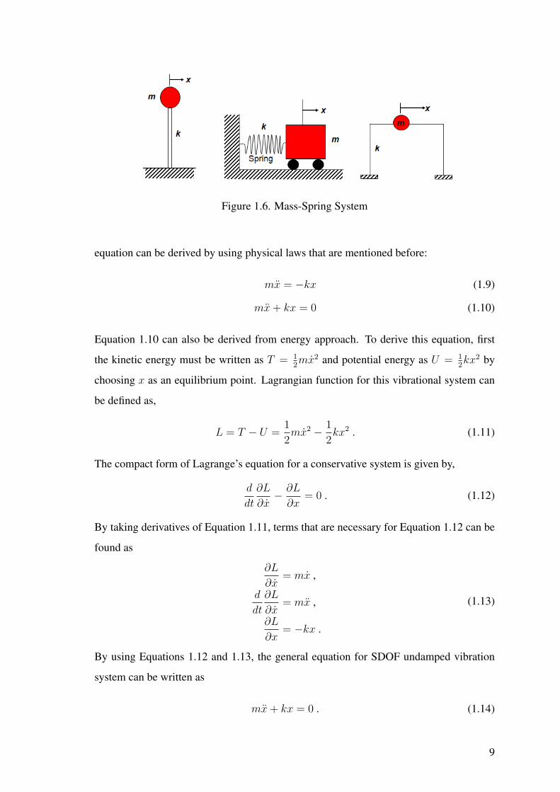
Figure 1.6. Mass-Spring System
equation can be derived by using physical laws that are mentioned before:
mx = −kx (1.9)
mx + kx = 0 (1.10)
Equation 1.10 can also be derived from energy approach. To derive this equation, first
the kinetic energy must be written as T = 12mx2 and potential energy as U = 1
2kx2 by
choosing x as an equilibrium point. Lagrangian function for this vibrational system can
be defined as,
L = T − U =1
2mx2 − 1
2kx2 . (1.11)
The compact form of Lagrange’s equation for a conservative system is given by,
d
dt
∂L
∂x− ∂L
∂x= 0 . (1.12)
By taking derivatives of Equation 1.11, terms that are necessary for Equation 1.12 can be
found as
∂L
∂x= mx ,
d
dt
∂L
∂x= mx ,
∂L
∂x= −kx .
(1.13)
By using Equations 1.12 and 1.13, the general equation for SDOF undamped vibration
system can be written as
mx + kx = 0 . (1.14)
9
Equation 1.10 is a linear, homogeneous 2nd order differential equation with constant co-
efficients. The solution of this equation for x(t) begins with assuming x(t) = est. By
writing the Equation 1.10 with this assumption,
m∂2est
∂t2+ kest = 0 , (1.15)
(ms2 + k)est = 0 . (1.16)
Since est cannot be equal to zero, (ms2 + k) must be equal to zero. The value of s can be
found as
[ms2 + k] = 0 , (1.17)
s1,2 =
√−k
m= ±jωn , (1.18)
ωn =
√k
m, (1.19)
where ωn is the natural frequency of the system in rad/s. General solution of differential
equation is,
x(t) = A1es1t + A2e
s2t = A1ejwnt + A2e
−jwnt . (1.20)
By using the relations
cos x =ejx + e−jx
2, (1.21)
sin x =ejx − e−jx
2j, (1.22)
Equation 1.20 can be written by means of cosine and sine functions,
x(t) = A cos ωnt + B sin ωnt . (1.23)
To find the coefficients A and B, the initial displacement and initial velocity of the mass
body must be known.
x(0) = A cos 0 + B sin 0 = A (1.24)
x(t) = −ωnA sin ωnt + ωnB cos ωnt (1.25)
x(0) = ωnB (1.26)
From Equations 1.24 and 1.26 , the coefficients A and B can be written by means of the
initial displacement and initial velocity.
A = x(0) (1.27)
B =x(0)
ωn
(1.28)
10

The solution of Equation 1.10 will be,
x(t) = A cos ωnt + B sin ωnt
= x(0) cos
√k
mt +
x(0)√km
sin
√k
mt . (1.29)
The graphical illustration of Equation 1.29 is shown in Figure 1.7. As shown in this
Figure 1.7. Free Vibration of SDOF Undamped System
figure, the amplitude of the free vibration response of an undamped system depends on
the initial displacement and velocity. Amplitude remains the same cycle after cycle and
motion does not decay because of the absence of damping.
The former equations describe the free vibration of the structure, however they
don’t explain why the system oscillates. The reason for oscillation is “conservation of
energy”. The conversion of potential energy in the spring and kinetic energy in the mass
creates these oscillations. In our model in Figure 1.6, the mass will continue to oscil-
late forever, but in a real system there is always damping that dissipates the energy and
therefore the system eventually comes to rest. Now assume that system also has a viscous
damper with damping value C as in Figure 1.8. C is equal to the damping force for a
unit velocity. Schematic diagrams in Figure 1.8 represents a damped SDOF vibrational
system with a single mass, a single spring and a single damper. The equation of motion
can be written as
F + Fc + Fk = 0 , (1.30)
mx(t) + cx(t) + kx(t) = 0 . (1.31)
11
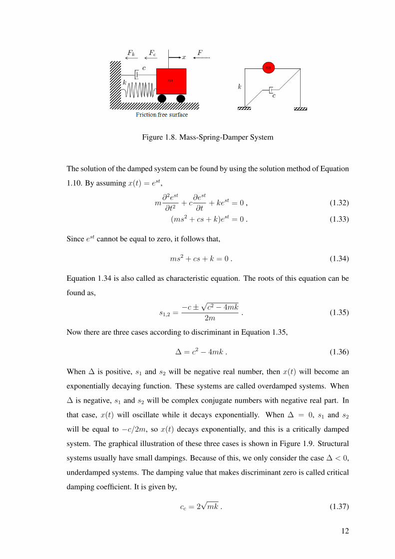
Figure 1.8. Mass-Spring-Damper System
The solution of the damped system can be found by using the solution method of Equation
1.10. By assuming x(t) = est,
m∂2est
∂t2+ c
∂est
∂t+ kest = 0 , (1.32)
(ms2 + cs + k)est = 0 . (1.33)
Since est cannot be equal to zero, it follows that,
ms2 + cs + k = 0 . (1.34)
Equation 1.34 is also called as characteristic equation. The roots of this equation can be
found as,
s1,2 =−c±√c2 − 4mk
2m. (1.35)
Now there are three cases according to discriminant in Equation 1.35,
∆ = c2 − 4mk . (1.36)
When ∆ is positive, s1 and s2 will be negative real number, then x(t) will become an
exponentially decaying function. These systems are called overdamped systems. When
∆ is negative, s1 and s2 will be complex conjugate numbers with negative real part. In
that case, x(t) will oscillate while it decays exponentially. When ∆ = 0, s1 and s2
will be equal to −c/2m, so x(t) decays exponentially, and this is a critically damped
system. The graphical illustration of these three cases is shown in Figure 1.9. Structural
systems usually have small dampings. Because of this, we only consider the case ∆ < 0,
underdamped systems. The damping value that makes discriminant zero is called critical
damping coefficient. It is given by,
cc = 2√
mk . (1.37)
12

Figure 1.9. Free Vibration of SDOF Damped System
Damping ratio of the system is defined as the ratio of damping value and critical damping
coefficient.
ξ =c
cc
=c
2√
mk(1.38)
Let us write Equation 1.35 as
s1,2 =−c
2m± j
√k
m− c2
4m2. (1.39)
In this equation the imaginary part of the root is usually referred as damped natural fre-
quency, given as,
ωd =
√k
m− c2
4m2. (1.40)
By using the damping ratio, the mathematical definition of damped natural frequency can
be written as,
ωd = ωn
√1− ξ2 . (1.41)
The real part of the roots can be written by means of natural frequency and damping factor
as,
ξωn =c
2m. (1.42)
Roots of the Equation 1.34 can be written as,
s1,2 = σ ± jωd = −ξωn ± jωd , (1.43)
13

where σ is the decay rate. The solution of Equation 1.31 is,
x(t) = eσt [A cos ωdt + B sin ωdt] . (1.44)
To find the coefficients A and B, the initial displacement and initial velocity of the mass
body must be known. From Equation 1.44:
x(0) = A cos 0 + B sin 0 = A
x(0) = −ωnA + ωdB .(1.45)
From Equation 1.45, the coefficients A and B can be written by means of the initial
displacement and initial velocity as,
A = x(0)
B =x(0)− σx(0)
ωd
.(1.46)
Therefore, the solution of the Equation 1.31 can be written as,
x(t) = eσt
[x(0) cos ωdt +
x(0)− σx(0)
ωd
sin ωdt
]. (1.47)
The graphical illustration of Equation 1.47 is shown in Figure 1.10. The comparison
between damped and undamped system can be seen from that figure. Coefficient p in
Figure 1.10. Comparison of Undamped System and Underdamped System
Figure 1.10 is magnitude of the solution. It can be derived as,
p =
√[x(0)]2 +
[x(0)− σx(0)
ωd
]2
. (1.48)
14
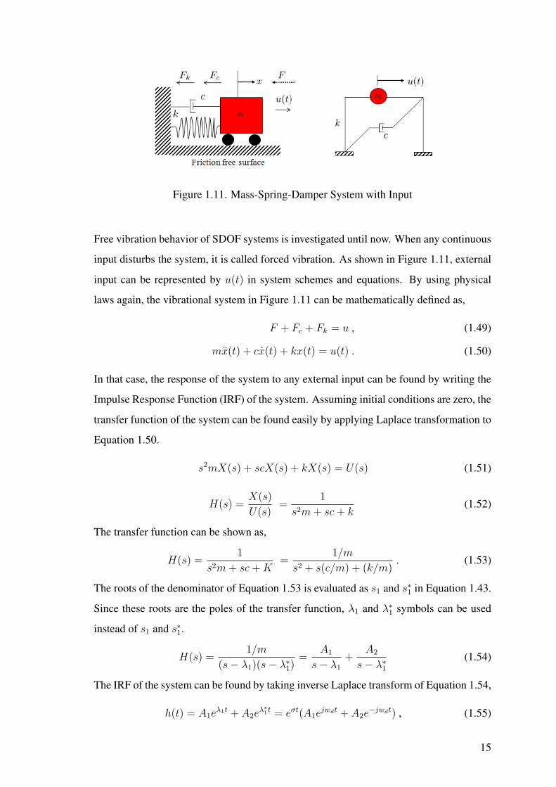
Figure 1.11. Mass-Spring-Damper System with Input
Free vibration behavior of SDOF systems is investigated until now. When any continuous
input disturbs the system, it is called forced vibration. As shown in Figure 1.11, external
input can be represented by u(t) in system schemes and equations. By using physical
laws again, the vibrational system in Figure 1.11 can be mathematically defined as,
F + Fc + Fk = u , (1.49)
mx(t) + cx(t) + kx(t) = u(t) . (1.50)
In that case, the response of the system to any external input can be found by writing the
Impulse Response Function (IRF) of the system. Assuming initial conditions are zero, the
transfer function of the system can be found easily by applying Laplace transformation to
Equation 1.50.
s2mX(s) + scX(s) + kX(s) = U(s) (1.51)
H(s) =X(s)
U(s)=
1
s2m + sc + k(1.52)
The transfer function can be shown as,
H(s) =1
s2m + sc + K=
1/m
s2 + s(c/m) + (k/m). (1.53)
The roots of the denominator of Equation 1.53 is evaluated as s1 and s∗1 in Equation 1.43.
Since these roots are the poles of the transfer function, λ1 and λ∗1 symbols can be used
instead of s1 and s∗1.
H(s) =1/m
(s− λ1)(s− λ∗1)=
A1
s− λ1
+A2
s− λ∗1(1.54)
The IRF of the system can be found by taking inverse Laplace transform of Equation 1.54,
h(t) = A1eλ1t + A2e
λ∗1t = eσt(A1ejwdt + A2e
−jwdt) , (1.55)
15
λ1,2 = −σ ± jwd , (1.56)
where σ is the decay rate and wd is the damped natural frequency.
The main objective of this study is to estimate the values of wd and σ from the measure-
ments. Besides that Civil engineers are also interested in the values of m, c, and k.
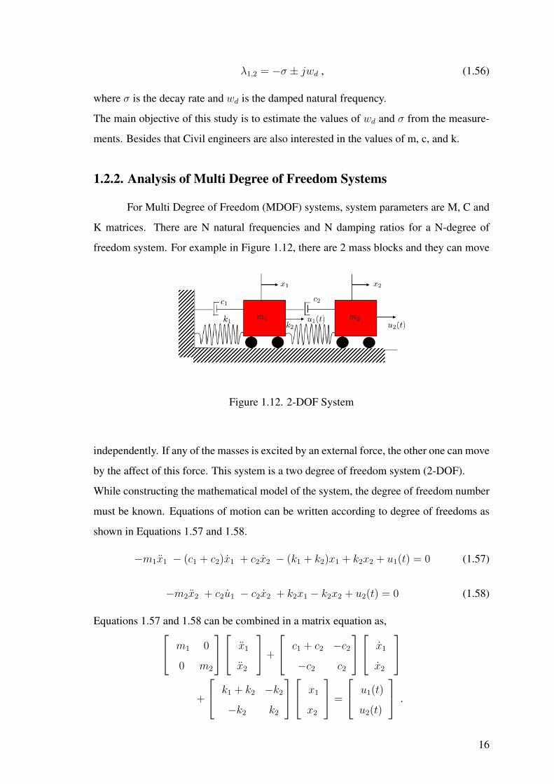
1.2.2. Analysis of Multi Degree of Freedom Systems
For Multi Degree of Freedom (MDOF) systems, system parameters are M, C and
K matrices. There are N natural frequencies and N damping ratios for a N-degree of
freedom system. For example in Figure 1.12, there are 2 mass blocks and they can move
Figure 1.12. 2-DOF System
independently. If any of the masses is excited by an external force, the other one can move
by the affect of this force. This system is a two degree of freedom system (2-DOF).
While constructing the mathematical model of the system, the degree of freedom number
must be known. Equations of motion can be written according to degree of freedoms as
shown in Equations 1.57 and 1.58.
−m1x1 − (c1 + c2)x1 + c2x2 − (k1 + k2)x1 + k2x2 + u1(t) = 0 (1.57)
−m2x2 + c2u1 − c2x2 + k2x1 − k2x2 + u2(t) = 0 (1.58)
Equations 1.57 and 1.58 can be combined in a matrix equation as, m1 0
0 m2
x1
x2
+
c1 + c2 −c2
−c2 c2
x1
x2
+
k1 + k2 −k2
−k2 k2
x1
x2
=
u1(t)
u2(t)
.
16
(1.59)
Equation 1.59 can be written as,
M x + Cx + Kx = u . (1.60)
MDOF damped vibrational systems can be defined by Equation 1.60. The transfer func-
tion of this 2-input, 2-output system can be written in a matrix form as,
H(s) =
H11(s) H12(s)
H21(s) H22(s)
, (1.61)
where Hij(s) for i, j = 1, 2, is the transfer function from ith input to jth output.
2-DOF system has 2 natural frequency and 2 modal damping factor as wd1, wd2 and σ1,
σ2. IRF of 2-DOF system can be written as,
h(t) =2∑
i=1
eσit(ai sin wdit + bi cos wdit) . (1.62)
Transfer function and IRF of MIMO vibrational systems can be generalized in a form
such that,
h(t) =N∑
i=1
eσit(ai sin wdit + bi cos wdit) , (1.63)
Hij(s) =N∑
r=1
[Aij(r)
s− sr
+A∗
ij(r)
s− s∗r
], (1.64)
where N is the number of degree of freedom in the system. Mathematically, our aim is to
find system parameters as wdi, σi in Equation 1.63 by using the measurement of h(t).
As mentioned before, natural frequency values can be easily calculated from dif-
ferential equations for SDOF systems. The solution for MDOF systems begins with un-
damped case. Equation 1.65 is a general equation for undamped vibrational systems. All
mass-spring systems can be defined by this equation.
M x(t) + Kx(t) = 0 (1.65)
The displacement response based on the nth mode can be given as,
x(t) = qn(t)φn , (1.66)
17

where qn(t) is the time variation of displacement and φn is the mode shape which does
not vary with time. qn(t) and φn can be written as,
qn(t) = An cos ωnt + Bn sin ωnt for n=1,2,..,N , (1.67)
φn =
φ1n
φ2n
.
.
φNn
. (1.68)
The displacement function can be written as,
x(t) = φn[An cos ωnt + Bn sin ωnt] . (1.69)
The second derivative of x(t), acceleration function, can be found easily from Equation
1.69.
x(t) =∂ [−φnAnωn sin ωnt + φnBnωn cos ωnt]
∂t
= −φnAnω2n cos ωnt− φnBnω
2n sin ωnt
= −φnω2nqn(t) (1.70)
By using Equation 1.65, 1.66 and 1.70,
M(−φnω2nqn(t)) + Kφnqn(t) = 0 , (1.71)
qn(t)[−ω2
nMφn + Kφn
]= 0 . (1.72)
Since qn(t) is the time variation of displacement, it can’t be zero, so [−ω2nMφn + Kφn]
will be equal to zero.
[−ω2nMφn + Kφn
]= 0 (1.73)
Kφn = ω2nMφn (1.74)
Equation 1.74 is a matrix eigenvalue problem and it can be written as,
[K − ω2
nM]φn = 0 . (1.75)
By using Equation 1.75, N equations for φjN (j=1,2,..,N) can be written. A homogeneous
system of N equations in N unknowns has a solution different from the obvious one, if
18
and only if the determinant of the coefficient matrix is zero. The solution of the Equation
1.75 exists if and only if
det[K − ω2
nM]
= 0 . (1.76)
This equation is called frequency equation, because natural frequencies can be found from
this equation. There are N real and positive roots for ω2n. Since the natural frequencies are
found, mode shapes, φn , can be found from Equation 1.75.
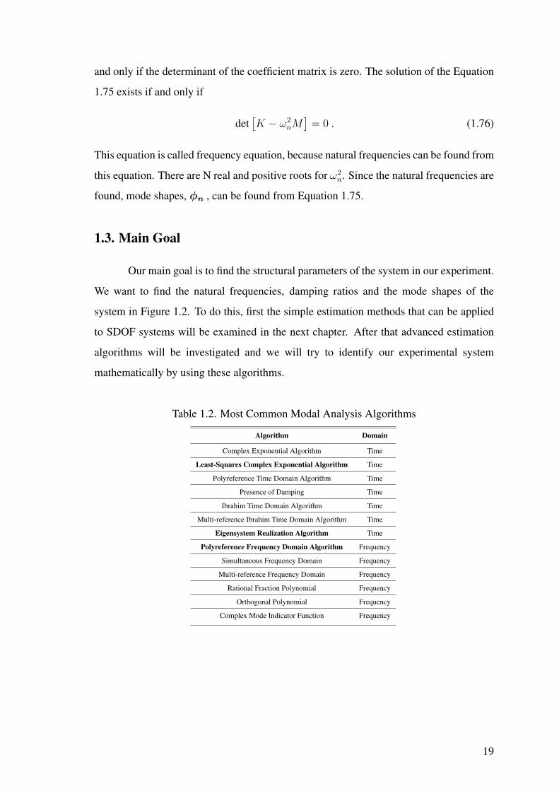
1.3. Main Goal
Our main goal is to find the structural parameters of the system in our experiment.
We want to find the natural frequencies, damping ratios and the mode shapes of the
system in Figure 1.2. To do this, first the simple estimation methods that can be applied
to SDOF systems will be examined in the next chapter. After that advanced estimation
algorithms will be investigated and we will try to identify our experimental system
mathematically by using these algorithms.
Table 1.2. Most Common Modal Analysis Algorithms
Algorithm Domain
Complex Exponential Algorithm Time
Least-Squares Complex Exponential Algorithm Time
Polyreference Time Domain Algorithm Time
Presence of Damping Time
Ibrahim Time Domain Algorithm Time
Multi-reference Ibrahim Time Domain Algorithm Time
Eigensystem Realization Algorithm Time
Polyreference Frequency Domain Algorithm Frequency
Simultaneous Frequency Domain Frequency
Multi-reference Frequency Domain Frequency
Rational Fraction Polynomial Frequency
Orthogonal Polynomial Frequency
Complex Mode Indicator Function Frequency
19

There are many advanced algorithms about system identification. In this study
algorithms in the literature is reviewed and the most common ones for our experiment is
listed in the Table 1.2.
Three fundamental and reliable algorithms are chosen from this list. We tried to
use two time-domain algorithms and one frequency-domain algorithm for the experimen-
tal data. These are the bold ones in the Table 1.2, “Least Squares Complex Exponential
(LSCE) Method ” , “Polyreference Frequency Domain Algorithm ” and “Eigensystem
Realization Algorithm ” . Initially, we will try to understand the theoretical background
of these methods. These methods will be verified for an artificial N degree of freedom
systems by using MATLAB simulations. Then these MATLAB scripts will be applied to
real measurement data and we will try to find the characteristic parameters of the system
in our experiment.
20
CHAPTER 2
SIMPLE ESTIMATION METHODS
2.1. Frequency Domain Estimation
In the first chapter, it was shown that the transfer function of a damped vibrational
system can be written as
H(s) =1/m
s2 + s(c/m) + (k/m)
=1/m
(s− λ1)(s− λ∗1)=
A1
s− λ1
+A2
s− λ∗1, (2.1)
where A1 and A2 are the residues of the transfer function. The residues of the transfer
function directly related to the amplitude of the IRF. By multiplying both sides of the
transfer function expression by s− λ1 and evaluating the result at s = λ1, residue A1 can
be found as
[ (s− λ1)H(s)] |s−λ1 = [ A1 +(s− λ1)A2
(s− λ∗1)] |s−λ1 ,
A1 =1/m
λ1 − λ∗1=
1/m
j2ω1
. (2.2)
By the same way, A2 can be found easily,
A2 =1/m
−j2ω1
. (2.3)
As shown in Equations 2.2 and 2.3, A1 and A2 are complex conjugates of each other, so
A∗1 can be written instead of A2. Transfer function can be written as
H(s) =A1
(s− λ1)+
A∗1
(s− λ∗1). (2.4)
By evaluating the transfer function along the jω axis, the frequency response of the system
can be found.
H(jω) =A1
(jω − λ1)+
A∗1
(jω − λ∗1)(2.5)
Experimentally when somebody is talking about measuring the transfer function, actually
the FRF is measured. At damped frequency, transfer function is such that,
H(jω1) =−A1
σ1
+A∗
1
(j2ω1 − σ1). (2.6)
21
Second term in Equation 2.6 approaches zero when ω1 gets large. H(ω1) can be repre-
sented as
H(ω1) =−A1
σ1
. (2.7)
Frequency response of SDOF system can be represented as
H(ω) =A1
jω − λ1
. (2.8)
Assuming that our system is a lightly damped SDOF system, parameters needed for a par-
tial fraction model can be estimated directly from the measured FRF. While this approach
is based upon a SDOF system, as long as the modal frequencies are not too close together,
the method can be used for multiple degree of freedom (MDOF) systems as well.
As shown in Equation 2.5, A1 and λ1 must be estimated to identify the FRF. Since
λ1 = σ1 + jω1 , decay rate and the natural frequency of the system must be estimated to
find the pole of the transfer function.
The estimation process begins with estimating the damped natural frequency, ω1. Damped
natural frequency could be estimated in one of three ways :
1)Damped natural frequency is the frequency where magnitude of FRF reaches maxi-
mum.
2)Damped natural frequency is the frequency where the real part of FRF crosses zero.
3)Damped natural frequency is the frequency where imaginary part of FRF reaches a rel-
ative minima or maxima.
The last approach generally gives the most reliable results. The estimation process can
be shown by an example simulation on MATLAB environment. Assume that we have a
SDOF vibrational system which has a mass of 1 kg, 100 N/m spring constant and 1 Ns/m
damping coefficient value. The frequency response of this system is shown in Figure
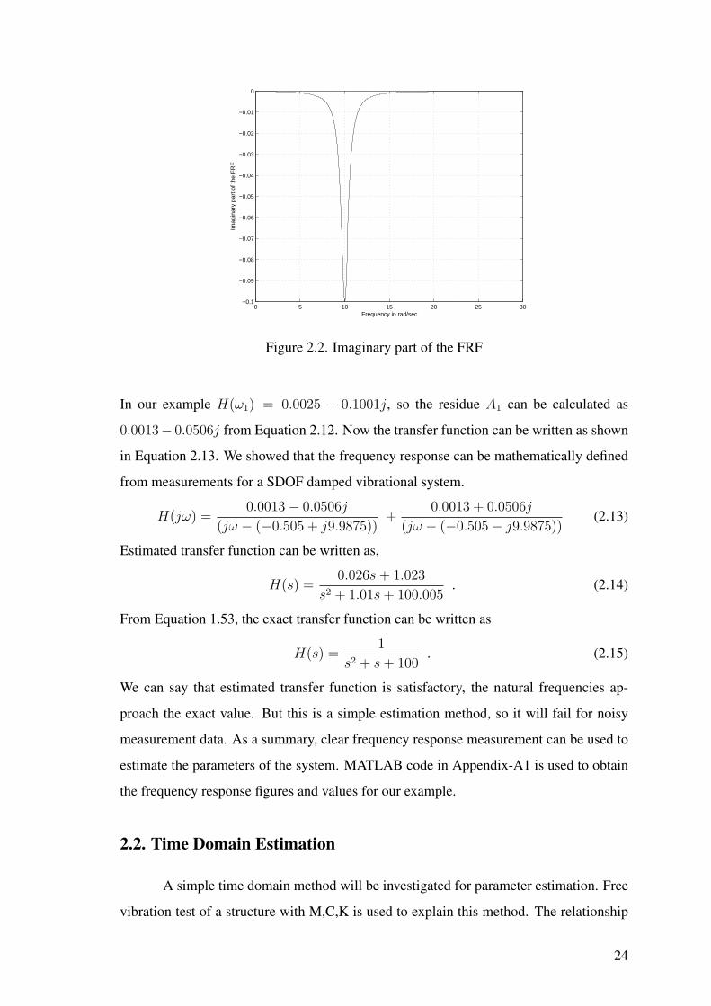
2.1 and 2.2. As shown in Figure 2.2, imaginary part of FRF reaches a relative minima
at nearly 10 rad/s. We can say that damped natural frequency of this system is equal to
10 rad/s from the frequency response of the system. Analytically, the real damped natural
frequency can be calculated as 9.9875 rad/s from Equation 1.40. Error is caused from the
sampling rate of the measurement device. Actually the damped natural frequency of the
system is 9.9875 rad/s but we saw that value as 10 rad/s.
Once the damped natural frequency w1 has been estimated, then the damping ratio ξ1 can
be estimated from the magnitude of the FRF. Damping ratio ξ1 can be estimated by using
22

0 5 10 15 20 25 30−0.06
−0.04
−0.02
0
0.02
0.04
0.06
Frequency in rad/sec
Rea
l par
t of t
he F
RF
Figure 2.1. Real part of the FRF
the half-power bandwidth method. This method uses the data from the FRF in the region
of the resonance frequency to estimate the fraction of critical damping from the formula:
ξ1 =ωb − ωa
2ω1
, (2.9)
where ω1 is the damped natural frequency as previously estimated. ωa is the frequency,
below ω1, where the magnitude is 0.707 of the peak magnitude of the FRF. This corre-
sponds to a half power point. ωb is the frequency, above ω1, where the magnitude is 0.707
of the peak magnitude of the FRF. This is also a half power point. For our example, we
can see that the half power frequency values are ωa = 9.46 rad/s and ωb = 10.47 rad/s.
Therefore the fraction of critical damping can be calculated from Equation 2.9 as 0.0506.
Once ξ1 is estimated, the decay rate, σ1 can be estimated as,
σ1 = −ξ1ω1 = 0.505 . (2.10)
The pole of the transfer function is λ1,2 = −0.505± j9.9875 . Once λ1,2 has been
estimated, the residue A1 can be estimated by evaluating the partial fraction model at a
specific frequency. If the specific frequency is chosen to be ω1, the following result is
obtained.
H(jω1) =A1
jω − (σ1 + jω1)+
A∗1
jω − (σ1 − jω1)(2.11)
As long as ω1 is not too small, the above equation could be approximated as,
H(ω1) =−A1
σ1
→ A1 ≈ (−σ1)H(ω1) . (2.12)
23
0 5 10 15 20 25 30−0.1
−0.09
−0.08
−0.07
−0.06
−0.05
−0.04
−0.03
−0.02
−0.01
0
Frequency in rad/sec
Imag
inar
y pa
rt o
f the
FR
F
Figure 2.2. Imaginary part of the FRF
In our example H(ω1) = 0.0025 − 0.1001j, so the residue A1 can be calculated as
0.0013− 0.0506j from Equation 2.12. Now the transfer function can be written as shown
in Equation 2.13. We showed that the frequency response can be mathematically defined
from measurements for a SDOF damped vibrational system.
H(jω) =0.0013− 0.0506j
(jω − (−0.505 + j9.9875))+
0.0013 + 0.0506j
(jω − (−0.505− j9.9875))(2.13)
Estimated transfer function can be written as,
H(s) =0.026s + 1.023
s2 + 1.01s + 100.005. (2.14)
From Equation 1.53, the exact transfer function can be written as
H(s) =1
s2 + s + 100. (2.15)
We can say that estimated transfer function is satisfactory, the natural frequencies ap-
proach the exact value. But this is a simple estimation method, so it will fail for noisy
measurement data. As a summary, clear frequency response measurement can be used to
estimate the parameters of the system. MATLAB code in Appendix-A1 is used to obtain
the frequency response figures and values for our example.
2.2. Time Domain Estimation
A simple time domain method will be investigated for parameter estimation. Free
vibration test of a structure with M,C,K is used to explain this method. The relationship
24

0 5 10 15 20 25 300
0.02
0.04
0.06
0.08
0.1
0.12
Frequency in rad/sec
Mag
nitu
de o
f the
FR
F
Figure 2.3. Magnitude of the FRF
between the damped and undamped natural frequency is known. Since TD = 2πωd
From
Equation 1.41, the relationship between the damped and undamped natural period can be
written as,
TD =Tn√1− ξ2
. (2.16)
Two consecutive peaks from the acceleration response data of the structure will be used
for estimation. Assume that the first peak is at time t, then the next peak must be at time
t + TD. By using Equation 1.44, the ratio of the acceleration function at these two time
instants can be taken and the Equation 2.17 can be derived easily.
x(t)
x(t + TD)= exp(ξωnTD) = exp(
2πξ√1− ξ2
) (2.17)
If the peaks in the time domain response is numbered as ith, i + 1th peak, one can write
that,
xi
xi+1
= exp(2πξ√1− ξ2
) . (2.18)
The natural logarithm of the ratio in Equation 2.18 is called the logarithmic decrement
which is denoted by δ.
δ = lnxi
xi+1
=2πξ√1− ξ2
(2.19)
Since the damping ratio is so small, the term of√
1− ξ2 will be approximately one. The
logarithmic decrement, δ will be,
δ = 2πξ . (2.20)
25
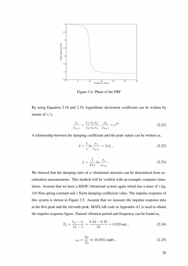
0 5 10 15 20 25 30−3.5
−3
−2.5
−2
−1.5
−1
−0.5
0
Frequency in rad/sec
Pha
se A
ngle
of t
he F
RF
Figure 2.4. Phase of the FRF
By using Equation 2.18 and 2.19, logarithmic decrement coefficient can be written by
means of xi’s.
x1
xj+1
=x1
x2
x2
x3
x3
x4
...xk
xk+1
= ekδ (2.21)
A relationship between the damping coefficient and the peak values can be written as,
δ =1
jln
x1
xj+1
= 2πξ , (2.22)
ξ =1
2πjln
xi
xi+j
. (2.23)
We showed that the damping ratio of a vibrational structure can be determined from ac-
celeration measurements. This method will be verified with an example computer simu-
lation. Assume that we have a SDOF vibrational system again which has a mass of 1 kg,
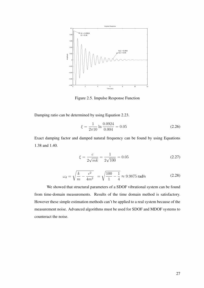
100 N/m spring constant and 1 Ns/m damping coefficient value. The impulse response of
this system is shown in Figure 2.5. Assume that we measure the impulse response data
at the first peak and the eleventh peak. MATLAB code in Appendix-A1 is used to obtain
the impulse response figure. Natural vibration period and frequency can be found as,
Td =t11 − t111− 1
=6.44− 0.16
10= 0.628 sec , (2.24)
ωd =2π
Td
≈ 10.0051 rad/s . (2.25)
26
0 2 4 6 8 10 12−0.08
−0.06
−0.04
−0.02
0
0.02
0.04
0.06
0.08
0.1
Impulse Response
Time (sec)
Am
plitu
de
h1 = 0.0924t1 = 0.16
h11 = 0.004t11 = 6.44
Figure 2.5. Impulse Response Function
Damping ratio can be determined by using Equation 2.23.
ξ =1
2π10ln
0.0924
0.004= 0.05 (2.26)
Exact damping factor and damped natural frequency can be found by using Equations
1.38 and 1.40.
ξ =c
2√
mk=
1
2√
100= 0.05 (2.27)
ωd =
√k
m− c2
4m2=
√100
1− 1
4≈ 9.9875 rad/s (2.28)
We showed that structural parameters of a SDOF vibrational system can be found
from time-domain measurements. Results of the time domain method is satisfactory.
However these simple estimation methods can’t be applied to a real system because of the
measurement noise. Advanced algorithms must be used for SDOF and MDOF systems to
counteract the noise.
27

CHAPTER 3
PRE-PROCESSING TECHNIQUES
Before applying system identification algorithms, some pre-processing techniques
must be applied to experimental measurements. By using these techniques, noise in mea-
surements can be reduced, then the IRF or FRF data of the system can be found clearly.
Windowing, averaging, filtering are the main pre-processing techniques.
The experimental system in this study is a single-input multi-output(SIMO) system. We
repeated the experiment 5 times and we obtained 5 input-output data pair for each ref-
erence point. Acceleration measurements are taken from 10 reference point. At the end
of the experiment, we had 50 measurement files. By using all of these data files and
pre-processing techniques, IRF or FRF estimate of each data pair can be found.
3.1. Frequency Domain Division Method
To eliminate the noise from input data, we assumed that the noise signal is equal
to the input signal measurement after first 100 data points, as shown in Figure 3.1. By
Figure 3.1. Noise Estimation from Input Signal
taking the d.c. component of the noise signal and subtracting it from the input data, the
input data can be cleared from noise approximately.
After making a noise reduction, windowing process can be applied to input/output
data. Windowing is simply defined as multiplying the signal by a typical window func-
28
tion. This process is used to minimize edge effects that results in spectral leakage in the
FFT spectrum. Exponential window is used for measurement data in our experiment.
Mathematically this process can be given as,
xw(t) = x(t)e−(t/τ) , (3.1)
where τ is called the exponential time constant. Also σ = 1/τ is called as damping or
decay rate. Generally decay rate is selected as,
σ = − ln(w(T )
T, (3.2)
where w(T ) is the value of exponential window at the end of analyzer’s time record and
T is analyzer’s time record length.
To find the FRF’s of each input-output pair, FFT of the input and the output data
can be taken by using MATLAB. Then FRF of each pair can be found by,
H(f) =Re[X(f)X∗(f)]
Y (f)X∗(f). (3.3)
By averaging all FRF’s of one reference point, the error in the estimate of the FRF’s can
be reduced. Then impulse response data of the system can be obtained by using inverse
FFT transform.
h(t) = IFT {H(f)} (3.4)
Pre-processing part of the study can be shown in a block diagram as in Figure 3.2.
Instead of division in frequency domain, an alternative method can be used to es-
timate the FRF. The autocorrelation and cross-correlation functions of input and output
data can be used to obtain a FRF estimation. The autocorrelation function and cross cor-
relation function are the inverse Fourier transforms of power spectral density and cross
spectral density of the input/output signals. The relation of correlation and spectral den-
sity functions can be given as,
SXY (f) = F{RXY (τ)} , (3.5)
SY Y (f) = F{RY Y (τ)} . (3.6)
By dividing the power spectral density of output signal by cross power spectral density of
input and output, the estimate of FRF can be obtained.
SXY (f) = H∗(f)SX(f) SY Y (f) = H∗(f)H(f)SX(f) (3.7)
H(f) =SY Y (f)
SXY (f)(3.8)
29
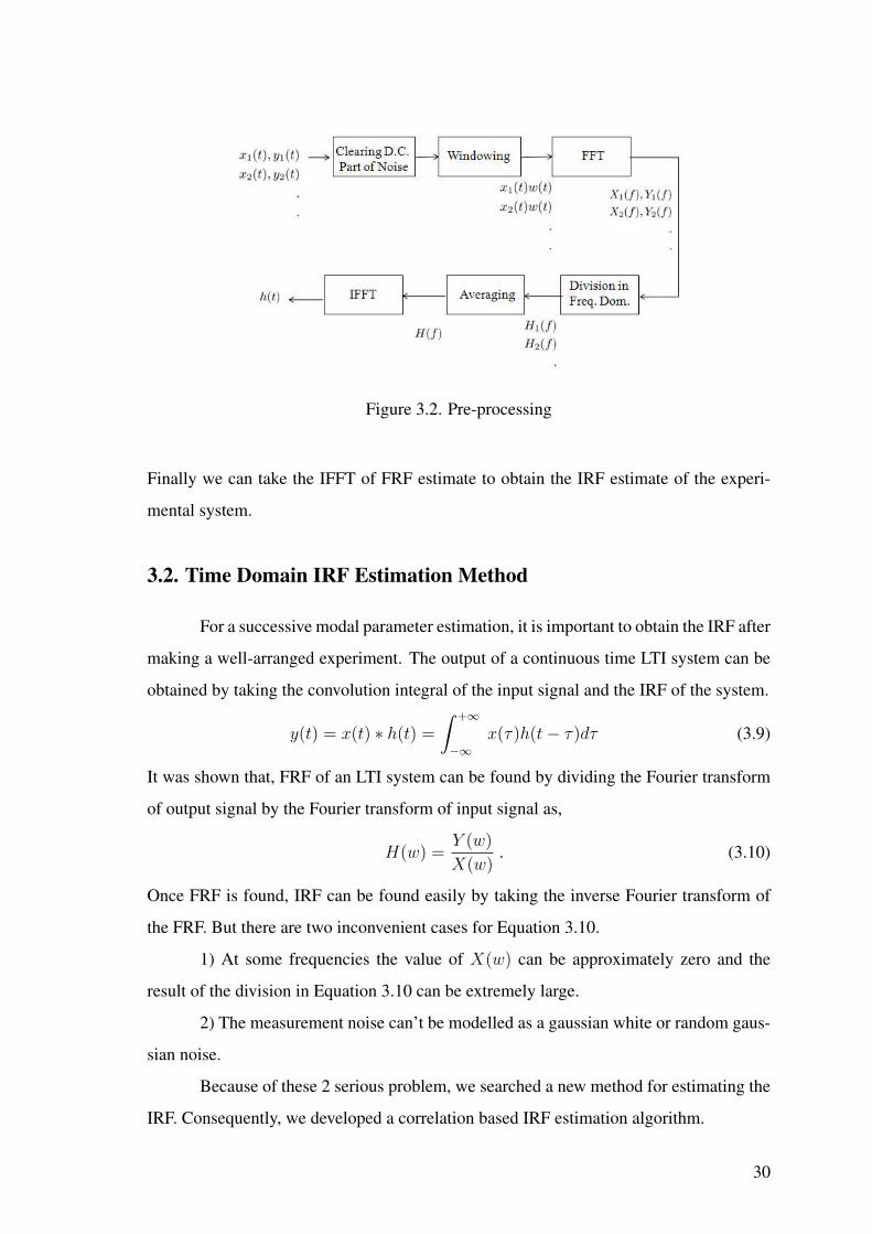
Figure 3.2. Pre-processing
Finally we can take the IFFT of FRF estimate to obtain the IRF estimate of the experi-
mental system.
3.2. Time Domain IRF Estimation Method
For a successive modal parameter estimation, it is important to obtain the IRF after
making a well-arranged experiment. The output of a continuous time LTI system can be
obtained by taking the convolution integral of the input signal and the IRF of the system.
y(t) = x(t) ∗ h(t) =
∫ +∞
−∞x(τ)h(t− τ)dτ (3.9)
It was shown that, FRF of an LTI system can be found by dividing the Fourier transform
of output signal by the Fourier transform of input signal as,
H(w) =Y (w)
X(w). (3.10)
Once FRF is found, IRF can be found easily by taking the inverse Fourier transform of
the FRF. But there are two inconvenient cases for Equation 3.10.
1) At some frequencies the value of X(w) can be approximately zero and the
result of the division in Equation 3.10 can be extremely large.
2) The measurement noise can’t be modelled as a gaussian white or random gaus-
sian noise.
Because of these 2 serious problem, we searched a new method for estimating the
IRF. Consequently, we developed a correlation based IRF estimation algorithm.
30
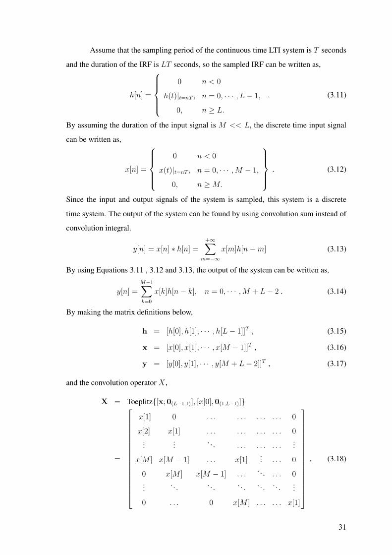
Assume that the sampling period of the continuous time LTI system is T seconds
and the duration of the IRF is LT seconds, so the sampled IRF can be written as,
h[n] =
0 n < 0
h(t)|t=nT , n = 0, · · · , L− 1,
0, n ≥ L.
. (3.11)
By assuming the duration of the input signal is M << L, the discrete time input signal
can be written as,
x[n] =
0 n < 0
x(t)|t=nT , n = 0, · · · ,M − 1,
0, n ≥ M.
. (3.12)
Since the input and output signals of the system is sampled, this system is a discrete
time system. The output of the system can be found by using convolution sum instead of
convolution integral.
y[n] = x[n] ∗ h[n] =+∞∑
m=−∞x[m]h[n−m] (3.13)
By using Equations 3.11 , 3.12 and 3.13, the output of the system can be written as,
y[n] =M−1∑
k=0
x[k]h[n− k], n = 0, · · · ,M + L− 2 . (3.14)
By making the matrix definitions below,
h = [h[0], h[1], · · · , h[L− 1]]T , (3.15)
x = [x[0], x[1], · · · , x[M − 1]]T , (3.16)
y = [y[0], y[1], · · · , y[M + L− 2]]T , (3.17)
and the convolution operator X ,
X = Toeplitz{[x;0(L−1,1)], [x[0],0(1,L−1)]}
=
x[1] 0 . . . . . . . . . . . . 0
x[2] x[1] . . . . . . . . . . . . 0...
... . . . . . . . . . . . ....
x[M ] x[M − 1] . . . x[1]... . . . 0
0 x[M ] x[M − 1] . . .. . . . . . 0
... . . . . . . . . . . . . . . . ...
0 . . . 0 x[M ] . . . . . . x[1]
, (3.18)
31

Equation 3.14 can be written as a matrix equation,
y = Xh , (3.19)
where y is the sampled response of the system, h is the impulse response vector and X
is the convolution matrix. The important point at Equation 3.19 is only h is unknown,
output and the input signal can be measured.
To estimate the impulse response vector of the system, the observation of the input can be
used. For this reason, the correlation of the input and output signal can be written as,
xcorr{x[n], y[n]} = XTy = XTXh . (3.20)
From Equation 3.20, estimate of IRF can be given as,
h = (XTX)−1XTy , (3.21)
which is known as the least squares estimate of the system impulse response (Louis L.
Scharf 2001).
Input signal in our experiment is taken as a dirac delta function. Thus the rightmost
term in the Equation 3.20, XTXh can be taken as a multiplication of impulse response
vector by a scalar. The Equation 3.20 can be written as,
XTy = XTXh ≈ αIh = αh . (3.22)
The approximation in Equation 3.22 is acceptable when the input signal is obtained by
“hitting a hammer ”which closely resembles a Dirac Delta function. Note that the approx-
imation in Equation 3.22 becomes an equality when the input signal is a perfect Dirac
Delta function. The term of XTX is the autocorrelation of the input signal x[n], and this
can be represented by a diagonal matrix αI where α is the total energy of the input signal
x[n]. This relation can be shown as,
α = XTX =M−1∑
k=0
x2[k] . (3.23)
By using Equation 3.22, an estimate of impulse response of the system can be written as,
h =1
αXTy . (3.24)
In each case, Equation 3.21 gives more reliable results than Equation 3.24, because there
must be an approximation error from Equation 3.22. We compared the results of these
two equations in the next section.
32
By using the estimates of the impulse response in Equation 3.24 and Equation
3.21, inconvenient cases in Equation 3.10 are solved. Now any parameter estimation
algorithm can be applied to estimated impulse response data to find the parameters of the
system.
3.3. Comparison of IRF Estimation Methods
IRF of the structure which is obtained from experimental data by using IRF es-
timation methods explained in former sections. A MATLAB simulation is performed to
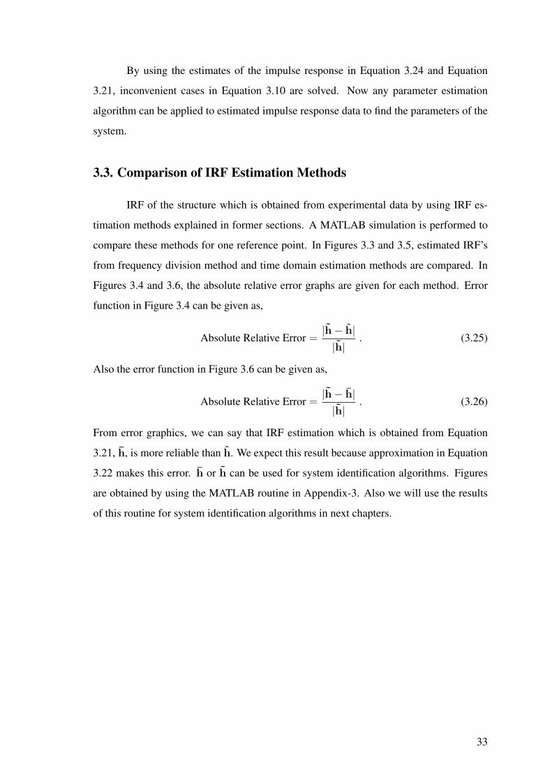
compare these methods for one reference point. In Figures 3.3 and 3.5, estimated IRF’s
from frequency division method and time domain estimation methods are compared. In
Figures 3.4 and 3.6, the absolute relative error graphs are given for each method. Error
function in Figure 3.4 can be given as,
Absolute Relative Error =|h− h||h| . (3.25)
Also the error function in Figure 3.6 can be given as,
Absolute Relative Error =|h− h||h| . (3.26)
From error graphics, we can say that IRF estimation which is obtained from Equation
3.21, h, is more reliable than h. We expect this result because approximation in Equation
3.22 makes this error. h or h can be used for system identification algorithms. Figures
are obtained by using the MATLAB routine in Appendix-3. Also we will use the results
of this routine for system identification algorithms in next chapters.
33
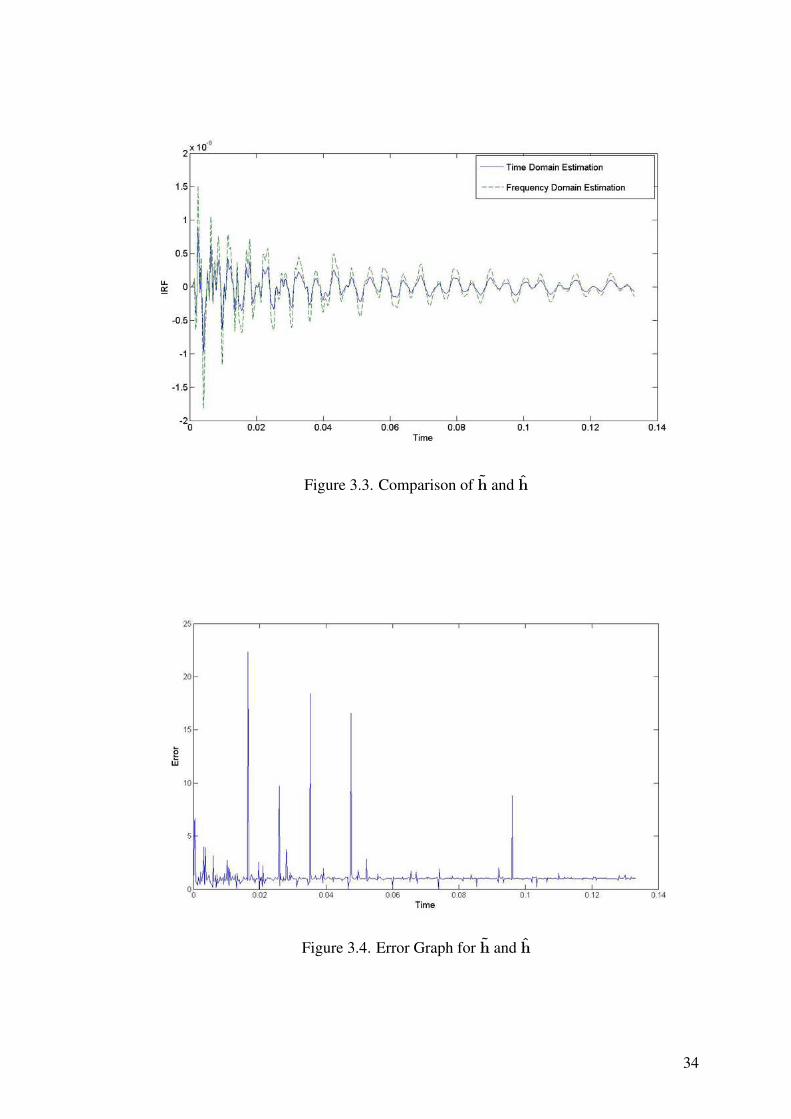
Figure 3.3. Comparison of h and h
Figure 3.4. Error Graph for h and h
34
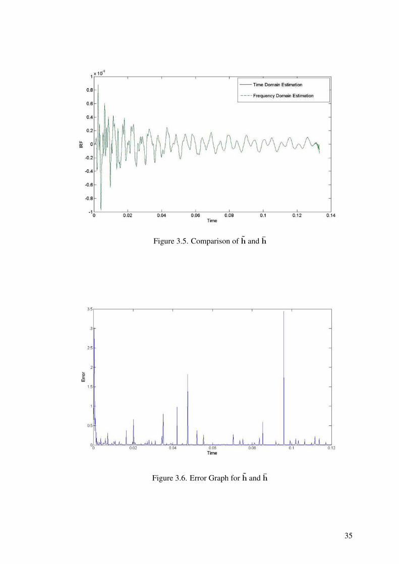
Figure 3.5. Comparison of h and h
Figure 3.6. Error Graph for h and h
35
CHAPTER 4
POLYREFERENCE FREQUENCY DOMAIN METHOD
4.1. State Space Representation
In order to understand the polyreference frequency domain method, state-space
concept and its applications to vibrational systems must be known. In this section the
state-space representation will be introduced and an example about a vibrational system
will be given.
State space representation is a mathematical description of a physical model. General
equations of this representation are,
˙x = Ax + Bu , (4.1)
y = Cx + Du , (4.2)
where,
x =
x1
.
.
xn
(4.3)
is the state vector which includes state variables as velocity or acceleration of a cart,
y =
y1
.
.
yq
(4.4)
is the output vector which includes outputs of the system, it can be the measurements in
an experiment,
u =
u1
.
.
up
(4.5)
36
is the input vector, which contains the inputs that are applied to the system. In this repre-
sentation A is called state matrix, B is called input matrix, C is called output matrix and
D is called feedforward matrix . By using Laplace transform, one can describe the whole
system with a rational transfer function. Derivation of the transfer function begins with
taking the Laplace transform of the state equation,
˙x = Ax + Bu , (4.6)
sX(s) = AX(s) + BU(s) , (4.7)
sX(s)− AX(s) = BU(s) , (4.8)
(sI − A)X(s) = BU(s) , (4.9)
X(s) = (sI − A)−1BU(s) . (4.10)
Equation 4.10 represents a relation between the input and the state. Another relation
between the input and the output can be written as,
y = Cx + Du , (4.11)
Y (s) = CX(s) + DU(s) , (4.12)
Y (s) = C(sI − A)−1BU(s) + DU(s) , (4.13)
Y (s) = [C(sI − A)−1B + D]U(s) . (4.14)
From Equation 4.14, the transfer function of the system can be written as,
H(s) =Y (s)
U(s), (4.15)
= [C(sI − A)−1B + D] . (4.16)
From Equation 4.16, it can be said that if A, B, C and D matrices is known, the transfer
function and IRF can be easily found. To understand the usage of state space representa-
tion for vibration systems, we will make an example for 2-DOF system in Figure 4.1. By
choosing the system states as the displacement and velocity of each cart,
x =
x1
x1
x2
x2
37
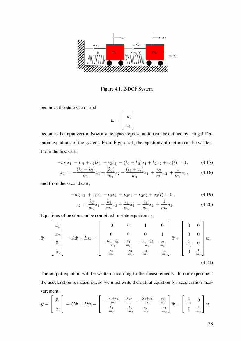
Figure 4.1. 2-DOF System
becomes the state vector and
u =
u1
u2
becomes the input vector. Now a state-space representation can be defined by using differ-
ential equations of the system. From Figure 4.1, the equations of motion can be written.
From the first cart;
−m1x1 − (c1 + c2)x1 + c2x2 − (k1 + k2)x1 + k2x2 + u1(t) = 0 , (4.17)
x1 = −(k1 + k2)
m1
x1 +(k2)
m1
x2 − (c1 + c2)
m1
x1 +c2
m1
x2 +1
m1
u1 , (4.18)
and from the second cart;
−m2x2 + c2u1 − c2x2 + k2x1 − k2x2 + u2(t) = 0 , (4.19)
x2 =k2
m2
x1 − k2
m2
x2 +c2
m2
x1 − c2
m2
x2 +1
m2
u2 . (4.20)
Equations of motion can be combined in state equation as,
˙x =
x1
x2
x1
x2
= Ax + Bu =
0 0 1 0
0 0 0 1
− (k1+k2)m1
(k2)m1
− (c1+c2)m1
c2m1
k2
m2− k2
m2
c2m2
− c2m2
x +
0 0
0 0
1m1
0
0 1m2
u .
(4.21)
The output equation will be written according to the measurements. In our experiment
the acceleration is measured, so we must write the output equation for acceleration mea-
surement.
y =
x1
x2
= Cx + Du =
− (k1+k2)
m1
(k2)m1
− (c1+c2)m1
c2m1
k2
m2− k2
m2
c2m2
− c2m2
x +
1m1
0
0 1m2
u
38
(4.22)
If the displacement response is measured instead of acceleration, output equation could
be written as,
y =
x1
x2
= Cx + Du =
1 0 0 0
0 0 1 0
x . (4.23)
Many advantages of state space representation is used in this study. This representation
will be used frequently in the Frequency Domain Algorithm section. Once the A,B, C
and D matrices is known, it is easy to find transfer function and IRF of the system. By
using these matrices, system’s response to any input can be found in time domain or
frequency domain. Furthermore, this representation is useful for constructing the math-
ematical model in MATLAB environment. As seen from the MATLAB programs in the
Appendices, the artificial mathematical models is created easily and by using these mod-
els the modal analysis algorithm is verified easily.
4.2. Frequency Domain Algorithm
In first chapter, it was shown that a linear mechanical system can be defined by
M x(t) + Cx(t) + Kx(t) = u(t) , (4.24)
where M , C and K are the mass, damping and stiffness matrices. For a time invariant
system , these matrices are constant and real. Vector x represents the displacement Then
x(t) and x(t) becomes velocity and acceleration. Transfer function of the system can be
written as,
H(s) =X(s)
U(s)=
output
input. (4.25)
If the external input, u, is a dirac delta function, laplace transform of input function will
be unity,
U(s) = 1 , (4.26)
then displacement response of the cart will be equal to the IRF.
H(jw) = X(jw) ⇐⇒ H(s) = X(s) ⇐⇒ h(t) = x(t) (4.27)
39
The Equation 4.24 can be written as,
M h(t) + Ch(t) + Kh(t) = uδ(t) . (4.28)
Since M is a non-singular matrix, by multiplying with M−1 each side of the Equation
4.28,
M−1M h(t) + M−1Ch(t) + M−1Kh(t) = M−1uδ(t) , (4.29)
h(t) + M−1Ch(t) + M−1Kh(t) = M−1uδ(t) . (4.30)
By setting A0 = M−1K , A1 = M−1C and B0 = M−1, Equation 4.30 can be written as,
h(t) = −A1h(t) − A0h(t) + B0uδ(t) . (4.31)
If the states of the system is chosen as
x =
h(t)
h(t)
, (4.32)
then a state-space representation can be written for our system. It is important to note
that x represents the state vector and x represents the displacement response, they are
different from each other.
˙x =
h(t)
h(t)
=
−A1 −A0
I 0
x +
B0
0
u (4.33)
Equation 4.33 is the state equation. In this equation, vector x represents the states and
vector u represents the inputs. To complete the state space representation, output must be
written. The output can be taken as the displacement of the structure.
y = h(t) =[
0 I]x (4.34)
Equation 4.34 is also called the observation equation. The state space representation of
the system defined in Equation 4.24 is obtained as
˙x = Ax + Bu
y = Cx , (4.35)
where A, B and C are given in Equations 4.33 and 4.34. Transfer function for the me-
chanical system can be written by using Equation 4.35 ,
H(s) = C[sI − A]−1B ⇐⇒ h(t) = CeAtB . (4.36)
40

The input-output relationship for a linear time-invariant system can be written as,
Y (s) = H(s)U(s) , (4.37)
y(t) = h(t) ∗ u(t) , (4.38)
where y(t) is output, u(t) is input and h(t) is the impulse response, note that ∗ is the
convolution operator and Y (s) = L{y(t)} , H(s) = L{h(t)} and U(s) = L{u(t)} .
Output of the system can be written as,
y(t) = CeAtBu(t) . (4.39)
By taking the derivative of Equation 4.39, y(t) and y(t) can be derived easily.
y(t) = CAeAtBu(t) + CeAtBu(t) (4.40)
L{y(t)} = sY (s)− y(0) (4.41)
y(t) = CA2eAtBu(t) + 2CAeAtBu(t) + CeAtBu(t) (4.42)
L{y(t)} = s2Y (s)− sy(0)− y(0) (4.43)
By applying Laplace transform to the Equation 4.31,
L{h(t)}+ A1L{h(t)}+ A0L{h(t)} = M−1 . (4.44)
To find L{h(t)} and L{h(t)} in Equation 4.44, the differentiation properties of Laplace
transform can be used.
df(t)
dt⇐⇒ sF (s)− f(0−) (4.45)
d2f(t)
dt2⇐⇒ s2F (s)− sf(0−)− f(0−) (4.46)
By setting L{h(t)} = H(s) and applying the Laplace properties in Equation 4.45 and
4.46 to Equation 4.36,
L{h(t)} = sH(s)− h(0−) = sH(s)− CB , (4.47)
L{h(t)} = s2H(s)− sh(0−)− h(0−) = s2H(s)− sCB − CAB . (4.48)
Lets consider the input-output relation of the mechanical system,
y(t) + A1y(t) + A0y(t) = M−1u(t) (4.49)
[ s2Y (s)− sy(0)− y(0) ] + A1[ sY (s)− y(0)] + A0Y (s) = M−1U (s) (4.50)
41

y(0) and y(0) must be evaluated to simplify the Equation 4.50 and to obtain the identifi-
cation equation.
y(0) = [CeAtBu(t)]t=0 = CBu(0) = 0 , (4.51)
since CB = 0.
y(0) = [ CAeAtBu(t) + CeAtBu(t) ]t=0 (4.52)
In Equation 4.52 the term [ CeAtBu(t) ]t=0 is taken as zero in the original article (Lem-
bregts and Leuridan 1990). But we found that that term is not zero, this error affects the
identification equation. To find the value of this term, a property and its proof is given,
Property :
eatδ(t)′ = −aδ(t) + δ(t)′ (4.53)
eAtδ(t)′ = −Aδ(t) + Iδ(t)′ (4.54)
Proof :∫ +∞
−∞f(t)δ′(t)dt = −
∫ +∞
−∞f ′(t)δ(t)dt = −f ′(0) (4.55)
∫ +∞
−∞φ(t)[eatδ′(t)]dt =
∫ +∞
−∞[φ(t)eat]δ′(t)dt (4.56)
= −[φ(t)aeat + φ(t)′eat]t=0 (4.57)
= −[φ(0)a + φ(0)′] (4.58)
= −∫
aφ(t)δ(t)dt +
∫φ(t)δ(t)′dt (4.59)
=
∫φ(t)[−aδ(t) + δ(t)′]dt (4.60)
The wrong term can be written as,
[ CeAtBu(t) ]t=0 = [ −CABu(0) + CBu(t) ]t=0
= −CABu(0) , (4.61)
since CB = 0. Then by putting this result to Equation 4.52,
y(0) = CABu(0)− CABu(0)
= 0 . (4.62)
42
Equation 4.50 can be written as,
s2Y (s) + A1sY (s) + A0Y (s) = M−1U(s) , (4.63)
[ s2I + A1s + A0]Y (s) = M−1U(s) . (4.64)
When input is dirac delta function, u(t) = δ(t), its laplace transform becomes U(s) = 1
and output will be the impulse response of the linear system.
[ s2I + A1s + A0]H(s) = M−1 (4.65)
In our experiment, the acceleration response of the system can be measured only, so the
system must be identified according to the acceleration measurements. Equation 4.65
must be written according to the acceleration transfer function, Ha(s). It was shown that
h(t) is the acceleration response, since h(t) is the displacement response. Let L{h(t)} =
Ha(s) = s2H(s), then
H(s) = Ha(s)/s2 , (4.66)
L{h(t)} = sH(s) = Ha(s)/s . (4.67)
By putting Equations 4.66 and 4.67 into equation 4.65,
Ha(s) + A1Ha(s)
s+ A0
Ha(s)
s2= M−1 , (4.68)
s2Ha(s) + A1sHa(s) + A0Ha(s) = s2M−1 , (4.69)
[ s2 + A1s + A0]Ha(s) = s2M−1 . (4.70)
By setting B0 = M−1 , the equation for identification can be completed as,
[s2I + A1s + A0]Ha(s) = s2B0 . (4.71)
There are 3 unknowns in Equation 4.71, A0, A1 and B0. To find these unknowns, least
square solution methods will be used. The Equation 4.71 can be written in frequency
domain, by setting s = jw,
[(jw)2I + A1jw + A0]Ha(jw) = (jw)2B0 . (4.72)
43
where j is the square root of−1 and w is the angular frequency. For s = jw1, jw2, ..., jwm
one can write that,
[ (jw1)2 + A1jw1 + A0]Ha(jw1) = (jw1)
2B0 (4.73)
[ (jw2)2 + A1jw2 + A0]Ha(jw2) = (jw2)
2B0
[ (jw3)2 + A1jw3 + A0]Ha(jw3) = (jw3)
2B0
.
.
.
Equation set 4.73 can be combined in a matrix notation.
[jwHa(jw) Ha(jw) −(jw)2
]
A1
A0
B0
= −(jw)2Ha(jw) (4.74)
Consequently, the matrix Equation 4.74 can be written as,
FG = H . (4.75)
Equation 4.74 is the last part of the identification. The exact value of F and H matrices
can be written easily from acceleration measurements. We want to find G matrix which
includes A1 , A0 and B0 . According to acceleration measurements, the row number of
F is much more than the column number. These systems are called as overdetermined
systems, equation number is much more than the number of unknowns. Generally these
systems can be solved by using least-square techniques like QR decomposition or Singu-
lar value decomposition. After solving G vector by least-square techniques, M , C and
K matrices and other system parameters can be easily calculated.
Derivation of the least-square approximation of the matrix Equation 4.75 is given be-
low. F is a m × n matrix and m ≥ n, so the inverse of this matrix can’t be taken. By
multiplying each side of the Equation 4.75 with F T ,
F T FG = F T H . (4.76)
Since F is a m× n matrix, F T F is a m×m matrix, and the inverse of this matrix can be
taken, then finding G matrix becomes possible.
[F T F ]−1[F T F ]G = [F T F ]−1F T H (4.77)
G = [F T F ]−1F T H (4.78)
44
The term [F T F ]−1F T is called the “pseudo inverse ”. Once matrix G is found, A1 , A0
and B0 can be written easily. It was shown that B0 = M−1, so mass matrix can be found.
If mass matrix is known, stiffness and damping matrices can be found from equations
A0 = M−1K and A1 = M−1C.
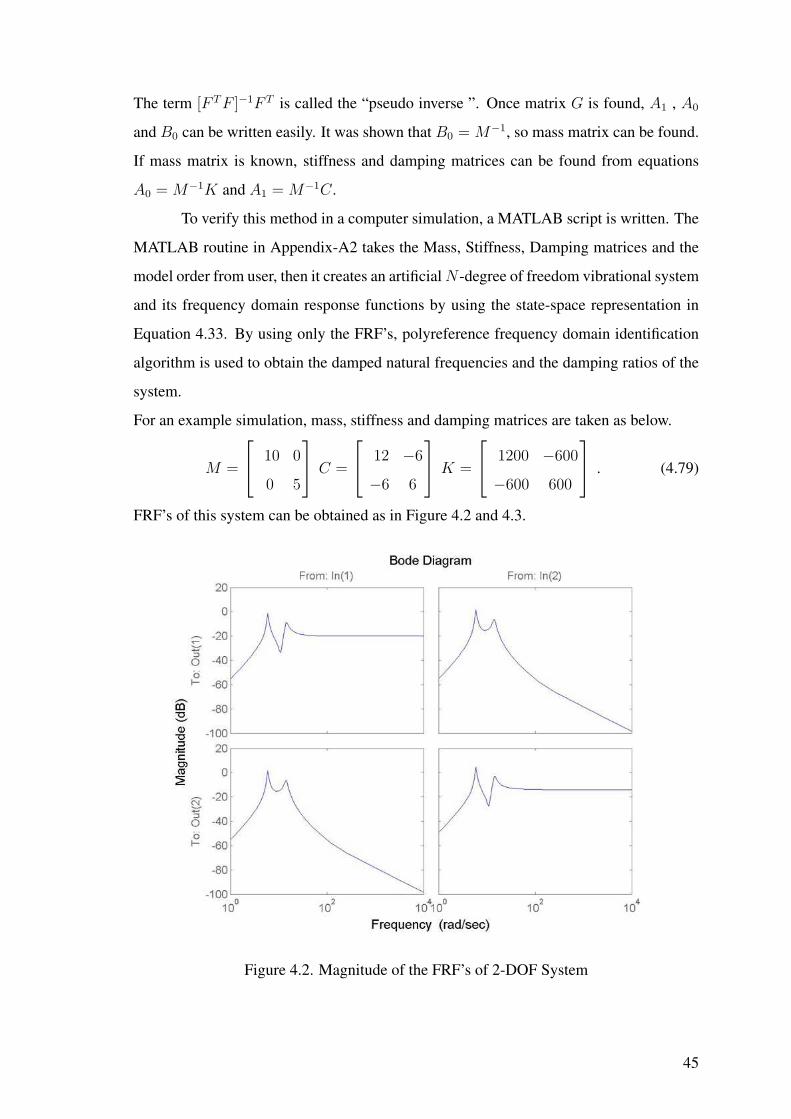
To verify this method in a computer simulation, a MATLAB script is written. The
MATLAB routine in Appendix-A2 takes the Mass, Stiffness, Damping matrices and the
model order from user, then it creates an artificial N -degree of freedom vibrational system
and its frequency domain response functions by using the state-space representation in
Equation 4.33. By using only the FRF’s, polyreference frequency domain identification
algorithm is used to obtain the damped natural frequencies and the damping ratios of the
system.
For an example simulation, mass, stiffness and damping matrices are taken as below.
M =
10 0
0 5
C =
12 −6
−6 6
K =
1200 −600
−600 600
. (4.79)
FRF’s of this system can be obtained as in Figure 4.2 and 4.3.
Figure 4.2. Magnitude of the FRF’s of 2-DOF System
45

By using the frequency response datas in Figure 4.2 and 4.3, the parameters of the
system can be extracted from PFD algorithm. The results of the MATLAB routine is in
the Table 4.1. Relative error in this table can be defined as,
Absolute Relative Error =|fexact − festimated|
fexact
. (4.80)
It can be said that from any FRF, the natural frequencies of the system can be extracted.
These results shows that, if the frequency response data of the system is measured clearly,
modal parameters of the system can be extracted by using PFD algorithm.
Figure 4.3. Phase of the FRF’s of 2-DOF System
Table 4.1. Results of PFD Simulation
Theoretical Natural Frequency Estimated Natural Frequency Relative Error
14.31268017327243 14.27598321867646 0, 0025
5.92850624167794 5.925901040354 0, 00044
46

After this verification, we tried to find the modal parameters of our experimental
material. First the time domain response and the input of the system is measured, then we
took the Fast Fourier Transform (FFT) of them. By dividing the frequency response of
the output and input, we found the FRF of the whole system. Then we applied the PFD
algorithm for this data. Estimated natural frequencies and damping ratios were not sat-
isfactory. Because of the noise in the measurement, we couldn’t successfully implement
the PFD algorithm for real measurement data. We decided to search any other advanced
algorithm for experimental data.
47

CHAPTER 5
LEAST SQUARES COMPLEX EXPONENTIAL
METHOD
As shown in Equation 1.64, a N-DOF MIMO system’s transfer function from ith
node to jth node can be written as,
Hij(s) =N∑
r=1
[Aij(r)
s− sr
+A∗
ij(r)
s− s∗r
]. (5.1)
For Aij(r) = A∗ij(r) and sr = s∗r , transfer function can be written as,
Hij(s) =2N∑r=1
Aij(r)
s− sr
. (5.2)
Then by using inverse Laplace transform, IRF of the system can be found as,
hij(t) =2N∑r=1
Aij(r)esrt . (5.3)
If this IRF is sampled by equally spaced time intervals k∆, we will have a discrete data
about the impulse response of the system. Actually at the end of the experiment, we have
only this discrete data. This data will be used to find the parameters of the system.
h(k∆) =2N∑r=1
Aij(r)esrk∆ (k = 0, 1, ...., 2N) (5.4)
By setting zr = esr∆, the IRF can be written as,
h[k] = h(k∆) =2N∑r=1
Aij(r)zkr (k = 0, 1, ...., 2N) . (5.5)
At this point a fitting method called Prony’s method will be used for the discrete impulse
response data. This method was developed by Gaspard Riche de Prony in 1795. Prony’s
method extracts valuable information from a uniformly sampled signal and builds a series
of damped complex exponentials or sinusoids. This allows for the estimation of fre-
quency, amplitude, phase and damping components of a signal. By using this method the
poles of the system can be found. First assume that zr is the solution of the polynomial,
β0 + β1zr + β2z2r + .... + β2N−1z
2N−1r + β2Nz2N
r = 0 (Prony Equation) . (5.6)
48
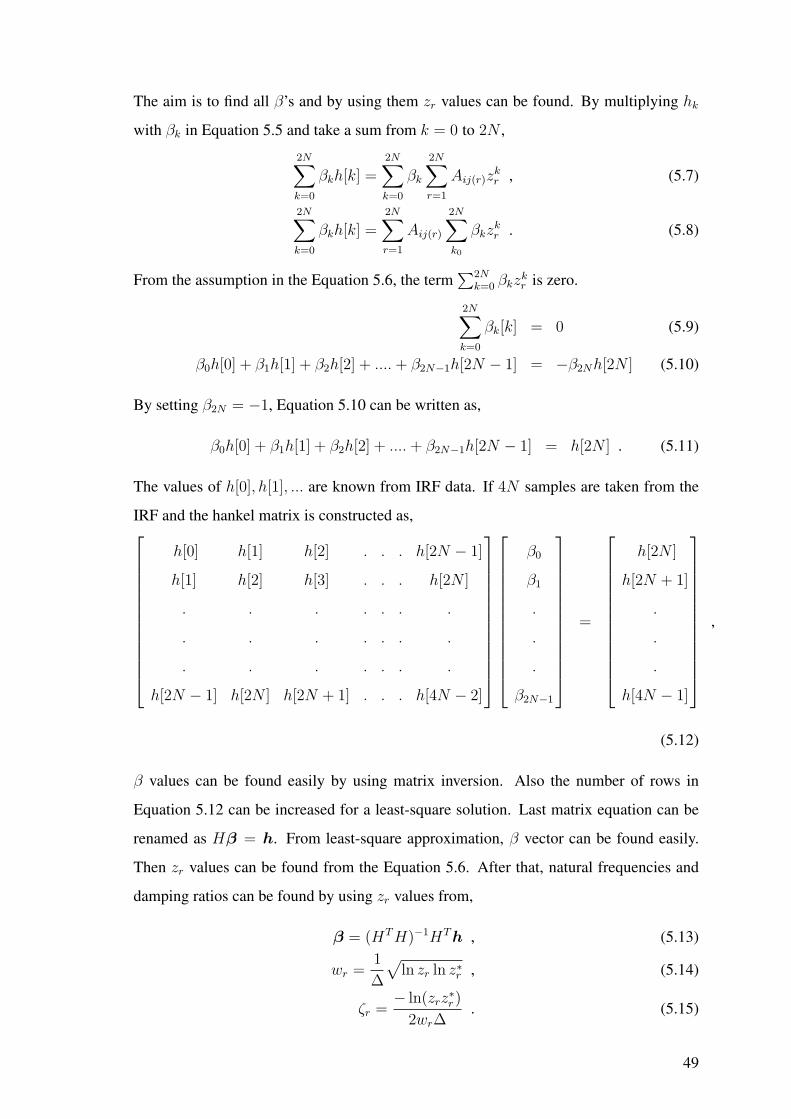
The aim is to find all β’s and by using them zr values can be found. By multiplying hk
with βk in Equation 5.5 and take a sum from k = 0 to 2N ,
2N∑
k=0
βkh[k] =2N∑
k=0
βk
2N∑r=1
Aij(r)zkr , (5.7)
2N∑
k=0
βkh[k] =2N∑r=1
Aij(r)
2N∑
k0
βkzkr . (5.8)
From the assumption in the Equation 5.6, the term∑2N
k=0 βkzkr is zero.
2N∑
k=0
βk[k] = 0 (5.9)
β0h[0] + β1h[1] + β2h[2] + .... + β2N−1h[2N − 1] = −β2Nh[2N ] (5.10)
By setting β2N = −1, Equation 5.10 can be written as,
β0h[0] + β1h[1] + β2h[2] + .... + β2N−1h[2N − 1] = h[2N ] . (5.11)
The values of h[0], h[1], ... are known from IRF data. If 4N samples are taken from the
IRF and the hankel matrix is constructed as,
h[0] h[1] h[2] . . . h[2N − 1]
h[1] h[2] h[3] . . . h[2N ]
. . . . . . .
. . . . . . .
. . . . . . .
h[2N − 1] h[2N ] h[2N + 1] . . . h[4N − 2]
β0
β1
.
.
.
β2N−1
=
h[2N ]
h[2N + 1]
.
.
.
h[4N − 1]
,
(5.12)
β values can be found easily by using matrix inversion. Also the number of rows in
Equation 5.12 can be increased for a least-square solution. Last matrix equation can be
renamed as Hβ = h. From least-square approximation, β vector can be found easily.
Then zr values can be found from the Equation 5.6. After that, natural frequencies and
damping ratios can be found by using zr values from,
β = (HT H)−1HT h , (5.13)
wr =1
∆
√ln zr ln z∗r , (5.14)
ζr =− ln(zrz
∗r )
2wr∆. (5.15)
49
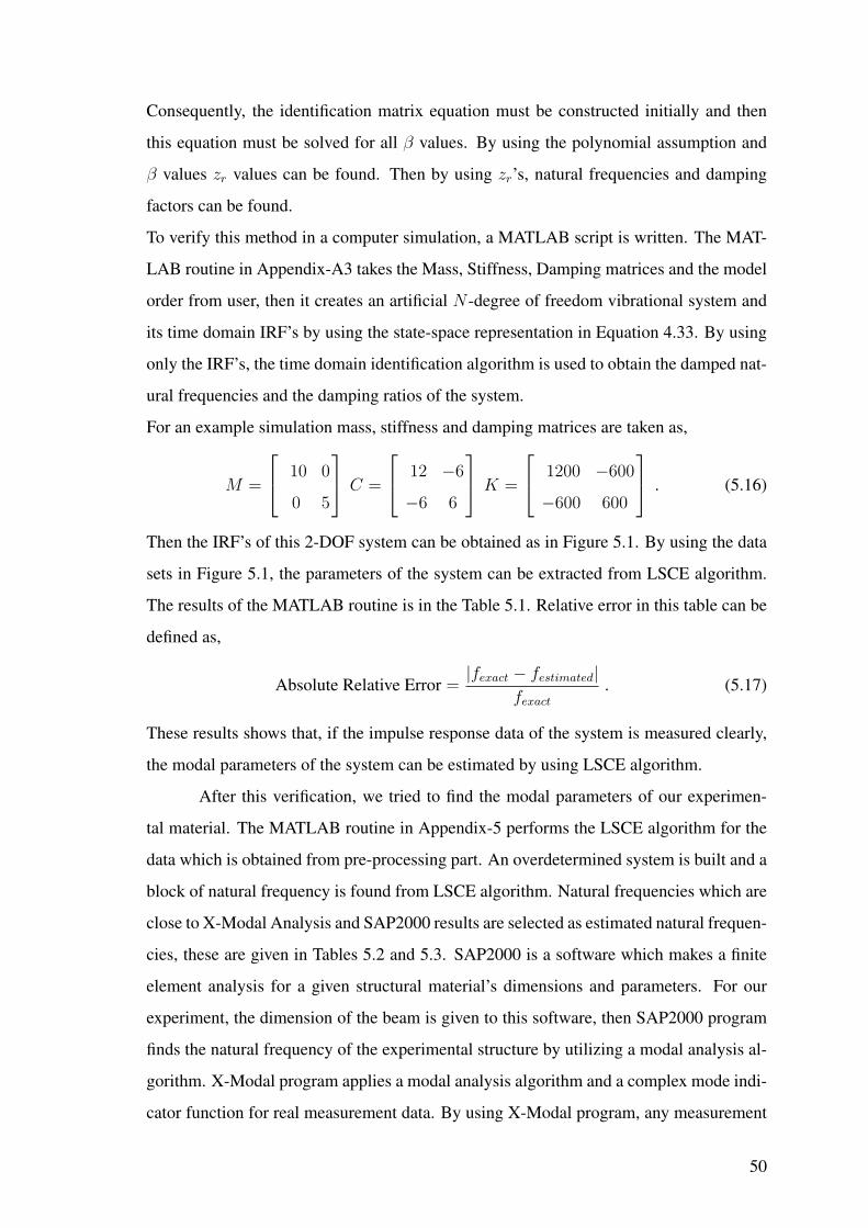
Consequently, the identification matrix equation must be constructed initially and then
this equation must be solved for all β values. By using the polynomial assumption and
β values zr values can be found. Then by using zr’s, natural frequencies and damping
factors can be found.
To verify this method in a computer simulation, a MATLAB script is written. The MAT-
LAB routine in Appendix-A3 takes the Mass, Stiffness, Damping matrices and the model
order from user, then it creates an artificial N -degree of freedom vibrational system and
its time domain IRF’s by using the state-space representation in Equation 4.33. By using
only the IRF’s, the time domain identification algorithm is used to obtain the damped nat-
ural frequencies and the damping ratios of the system.
For an example simulation mass, stiffness and damping matrices are taken as,
M =
10 0
0 5
C =
12 −6
−6 6
K =
1200 −600
−600 600
. (5.16)
Then the IRF’s of this 2-DOF system can be obtained as in Figure 5.1. By using the data
sets in Figure 5.1, the parameters of the system can be extracted from LSCE algorithm.
The results of the MATLAB routine is in the Table 5.1. Relative error in this table can be
defined as,
Absolute Relative Error =|fexact − festimated|
fexact
. (5.17)
These results shows that, if the impulse response data of the system is measured clearly,
the modal parameters of the system can be estimated by using LSCE algorithm.
After this verification, we tried to find the modal parameters of our experimen-
tal material. The MATLAB routine in Appendix-5 performs the LSCE algorithm for the
data which is obtained from pre-processing part. An overdetermined system is built and a
block of natural frequency is found from LSCE algorithm. Natural frequencies which are
close to X-Modal Analysis and SAP2000 results are selected as estimated natural frequen-
cies, these are given in Tables 5.2 and 5.3. SAP2000 is a software which makes a finite
element analysis for a given structural material’s dimensions and parameters. For our
experiment, the dimension of the beam is given to this software, then SAP2000 program
finds the natural frequency of the experimental structure by utilizing a modal analysis al-
gorithm. X-Modal program applies a modal analysis algorithm and a complex mode indi-
cator function for real measurement data. By using X-Modal program, any measurement
50
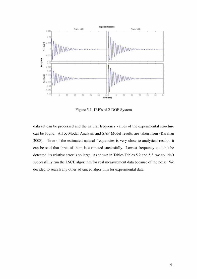
Figure 5.1. IRF’s of 2-DOF System
data set can be processed and the natural frequency values of the experimental structure
can be found. All X-Modal Analysis and SAP Model results are taken from (Karakan
2008). Three of the estimated natural frequencies is very close to analytical results, it
can be said that three of them is estimated succesfully. Lowest frequency couldn’t be
detected, its relative error is so large. As shown in Tables Tables 5.2 and 5.3, we couldn’t
successfully run the LSCE algorithm for real measurement data because of the noise. We
decided to search any other advanced algorithm for experimental data.
51
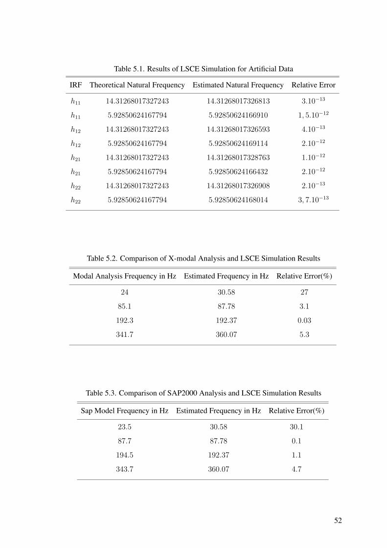
Table 5.1. Results of LSCE Simulation for Artificial Data
IRF Theoretical Natural Frequency Estimated Natural Frequency Relative Error
h11 14.31268017327243 14.31268017326813 3.10−13
h11 5.92850624167794 5.92850624166910 1, 5.10−12
h12 14.31268017327243 14.31268017326593 4.10−13
h12 5.92850624167794 5.92850624169114 2.10−12
h21 14.31268017327243 14.31268017328763 1.10−12
h21 5.92850624167794 5.92850624166432 2.10−12
h22 14.31268017327243 14.31268017326908 2.10−13
h22 5.92850624167794 5.92850624168014 3, 7.10−13
Table 5.2. Comparison of X-modal Analysis and LSCE Simulation Results
Modal Analysis Frequency in Hz Estimated Frequency in Hz Relative Error(%)
24 30.58 27
85.1 87.78 3.1
192.3 192.37 0.03
341.7 360.07 5.3
Table 5.3. Comparison of SAP2000 Analysis and LSCE Simulation Results
Sap Model Frequency in Hz Estimated Frequency in Hz Relative Error(%)
23.5 30.58 30.1
87.7 87.78 0.1
194.5 192.37 1.1
343.7 360.07 4.7
52
CHAPTER 6
EIGENSYSTEM REALIZATION ALGORITHM
One of the popular modal analysis techniques for civil structures is the eigensys-
tem realization algorithm. In this chapter a summary of this algorithm will be given and
after that the verification of the algorithm will be made by a MATLAB simulation. Jer-
Nan Juang and Richard Pappa developed ERA at the NASA Langley Research Center in
1985. ERA is a minimum order realization technique and it is an extension of the Ho-
Kalman algorithm that uses singular value decomposition technique for denoising. ERA
begins with the definition of the Markov parameter of a state-space model. Consider a
discrete time state space model such that,
x[k + 1] = Ax[k] + Bu[k]
y[k] = Cx[k] + Du[k] . (6.1)
To obtain the impulse response of the system, the input must be an impulse, it can be a
dirac delta. If u[k] = δ[k], the output y[k] will be the impulse response of the system
h[k]. If we start to write the h[k]’s beginning from the zero-state by assuming the system
is initially at rest,
h[0] = Cx[0] + Dδ[0] = D
x[1] = Ax[0] + Bδ[0] = B
h[1] = Cx[1] + Dδ[1] = CB
x[2] = Ax[1] + Bδ[1] = AB
h[2] = Cx[2] + Dδ[2] = CAB
h[3] = CA2B
.
.
h[n] = CAn−1B (6.2)
53
The impulse response of the system can be written as,
h[n] =
D, n = 0
CAn−1B, n > 0.. (6.3)
The term of CAn−1B is called the Markov parameter of the system. By using these
parameters one can define the impulse response of the system.
Y [k] = CAk−1B (6.4)
Consequently, the identification problem is: Given values of Y [k]’s, construct the constant
matrices A, B and C to identify the system. The algorithm begins by constructing a rxs
generalized Hankel matrix,
Hrs[k] =
Y [k] Y [k + t1] . . . . Y [k + ts−1]
Y [j1 + k] Y [j1 + k + t1] . . . . Y [j1 + k + ts−1]
. . . . . . .
. . . . . . .
. . . . . . .
Y [jr−1 + k] Y [jr−1 + k + t1] . . . . Y [jr−1 + k + ts−1]
.
(6.5)
where ji(i = 1, ..., r − 1) and ti(i = 1, ..., s − 1) are arbitrary integers. Controllability
and observability matrices of a state-space system can be written by using A, B and C
matrices as in,
Vr =
C
CAj1
CAj2
.
.
CAjr−1
, (6.6)
Ws = [B, At1B,At2B, ..., Ats−1B] , (6.7)
where Vr is the observability matrix and Ws is the controllability matrix. The Hankel ma-
trix in Equation 6.5 can be written by means of observability and controllability matrices
as,
Hrs[k] = VrAkWs . (6.8)
54
Assume that there exists a matrix H# satisfying the relation,
WsH#Vr = In , (6.9)
where In is an identity matrix of order n. From Equations 6.8 and 6.9,
Hrs[0]H#Hrs[0] = VrWsH#VrWs = VrWs = Hrs[0] . (6.10)
It can be said that H# is the pseudoinverse of the matrix Hrs[0].
H# = [[Hrs[0]]T [Hrs[0]]]−1[Hrs[0]]T (6.11)
Now a general solution for H# will be given. By writing the singular value decomposition
of Hrs[0] as,
Hrs[0] = PDQT , (6.12)
where D is a diagonal matrix which consists the singular values of Hrs[0]. By combining
the matrices P and D,
Hrs[0] = PDQT = [PD][QT ] = PdQT . (6.13)
The matrices Pd, QT , Ws and V Tr has rank and row number n. By using Equation 6.8
with k = 0,
VrWs = Hrs[0] = PdQT . (6.14)
Multiplying left side by P Td and solving for QT ,
TWs = (P Td Pd)
−1P Td VrWs = QT . (6.15)
Consider a U matrix such as,
U = WsQ(QT Q)−1 = WsQ . (6.16)
It can be seen that TU = I from Equations 6.15 and 6.16. T is nonsingular. By using the
relation TU = I and Equations 6.15 and 6.16,
Ws[Q(P Td Pd)
−1P Td ]Vr = In . (6.17)
Now matrix H# can be extracted as,
H# = [Q][(P Td Pd)
−1P Td ] = [Q][D−1P T ] = QP#
d . (6.18)
55

By defining ETp = [Ip, 0p, ..., 0p] and ET
m = [Im, 0m, ..., 0m] where 0p is a null matrix of
order p and Ip is an identity matrix of order p and by using Equations 6.8, 6.9 and 6.18, a
minimum order realization can be obtained.
Y [k + 1] = ETp Hrs[k]Em = ET
p VrAkWsEm
= ETp VrWsH
#VrAkWsH
#VrWsEm
= ETp Hrs[0]QP#
d VrAkWsQP#
d Hrs[0]Em
= ETp Hrs[0]Q[P#
d Hrs[1]Q]kP#d Hrs[0]Em
= ETp Pd[P
#d Hrs[1]Q]kQT Em
= ETp PD1/2[D−1/2P T Hrs[1]QD−1/2]kD1/2QT Em
The minimum order realization of the matrices [A,B,C] is
[D−1/2P T Hrs[1]QD−1/2, D1/2QT Em, ETp PD1/2]. The system in Equation 6.1 can
be written with these parameters,
x[k + 1] = D−1/2P T Hrs[1]QD−1/2x[k] + D1/2QT Emu[k]
y[k] = ETp PD1/2x[k] , (6.19)
where
x[k] = WsQD−1/2x[k] . (6.20)
Consequently, we can say that a discrete time LTI dynamical system can be identified
from the measurement functions if the system is controllable and observable. Matrices
Vr and Ws must be full rank for controllability and observability of the system. Natu-
ral frequencies and the damping ratios of the vibrational system can be found from the
eigenvalues of the realization of the matrix A. Remember that the imaginary part of the
eigenvalues of matrix A gives us the natural frequencies of the system.
To verify ERA in a computer simulation, a MATLAB script is written. The MAT-
LAB routine in Appendix-A4 takes the Mass, Stiffness, Damping matrices and the model
order from user, then it creates an artificial N -degree of freedom vibrational system and
its time domain IRF’s by using the state-space representation in Equation 4.33. By using
only the impulse response functions, ERA is used to obtain the damped natural frequen-
cies and the damping ratios of the system.
56

For an example simulation mass, stiffness and damping matrices are taken as,
M =
10 0
0 5
C =
12 −6
−6 6
K =
1200 −600
−600 600
. (6.21)
IRF’s of this 2-DOF system is given in Figure 5.1. By using the data sets in Figure
5.1 only, the parameters of the system can be extracted from ERA. The results of the
MATLAB routine is in the Table 6.1. Relative error in this table can be defined as,
Absolute Relative Error =|fexact − festimated|
fexact
. (6.22)
As shown, the natural frequencies and damping ratios of any system can be extracted
from any IRF. These results shows that, if we can measure the impulse response data
of the system clearly, we can extract the modal parameters of the system by using ERA
algorithm.
Table 6.1. Results of ERA Simulation for Artificial Data
IRF Theoretical Natural Frequency Estimated Natural Frequency Relative Error
h11 14.31268017327243 14.27598321866659 25.10−4
h11 5.92850624167794 5.92590104035906 4.10−4
Table 6.2. Comparison of X-modal Analysis and ERA Simulation Results
Modal Analysis Frequency in Hz Estimated Frequency in Hz Relative Error(%)
24 25.11 4.6
85.1 85.55 0.5
192.3 194.33 0.03
341.7 346.65 1.0
After this verification, we apply the ERA algorithm for experimental data in a
MATLAB simulation. An overdetermined system is built and a block of natural frequency
is found from LSCE algorithm. Some frequencies are eliminated by using a consistent
mode indicator function(Pappa and Elliott 1992), finally 4 natural frequency is found.
As shown in Tables 6.2 and 6.3, estimated natural frequencies were so close to analytical
results. In spite of the measurement noise, performance of the ERA is satisfactory. It can
be said that ERA is more effective than LSCE or PFD for noisy systems.
57
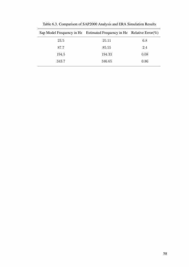
Table 6.3. Comparison of SAP2000 Analysis and ERA Simulation Results
Sap Model Frequency in Hz Estimated Frequency in Hz Relative Error(%)
23.5 25.11 6.8
87.7 85.55 2.4
194.5 194.33 0.08
343.7 346.65 0.86
58
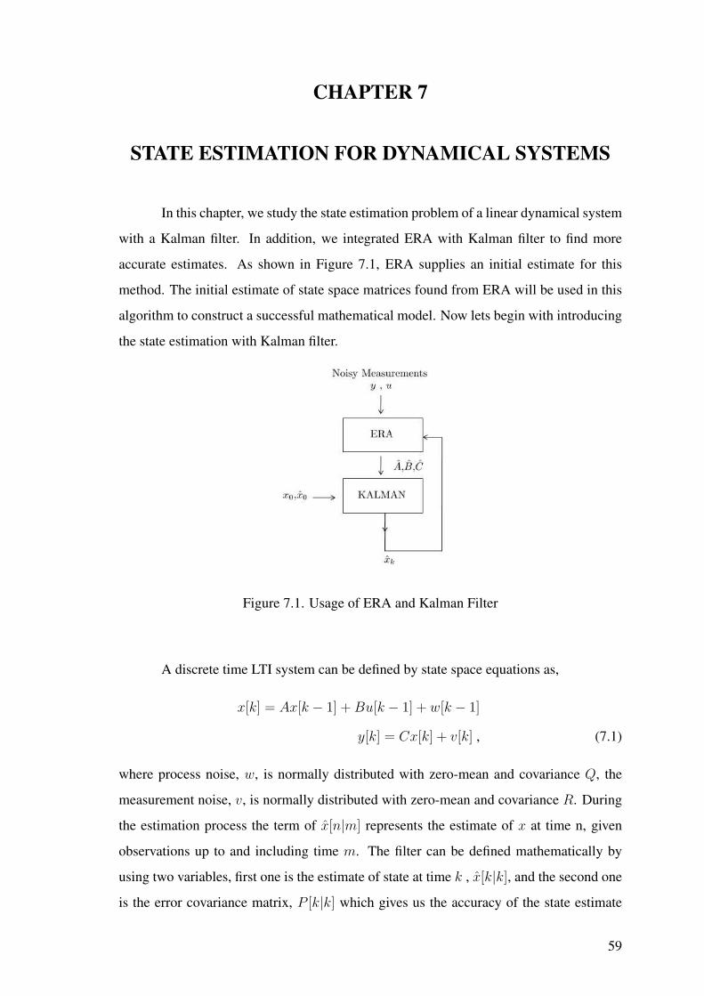
CHAPTER 7
STATE ESTIMATION FOR DYNAMICAL SYSTEMS
In this chapter, we study the state estimation problem of a linear dynamical system
with a Kalman filter. In addition, we integrated ERA with Kalman filter to find more
accurate estimates. As shown in Figure 7.1, ERA supplies an initial estimate for this
method. The initial estimate of state space matrices found from ERA will be used in this
algorithm to construct a successful mathematical model. Now lets begin with introducing
the state estimation with Kalman filter.
Figure 7.1. Usage of ERA and Kalman Filter
A discrete time LTI system can be defined by state space equations as,
x[k] = Ax[k − 1] + Bu[k − 1] + w[k − 1]
y[k] = Cx[k] + v[k] , (7.1)
where process noise, w, is normally distributed with zero-mean and covariance Q, the
measurement noise, v, is normally distributed with zero-mean and covariance R. During
the estimation process the term of x[n|m] represents the estimate of x at time n, given
observations up to and including time m. The filter can be defined mathematically by
using two variables, first one is the estimate of state at time k , x[k|k], and the second one
is the error covariance matrix, P [k|k] which gives us the accuracy of the state estimate
59
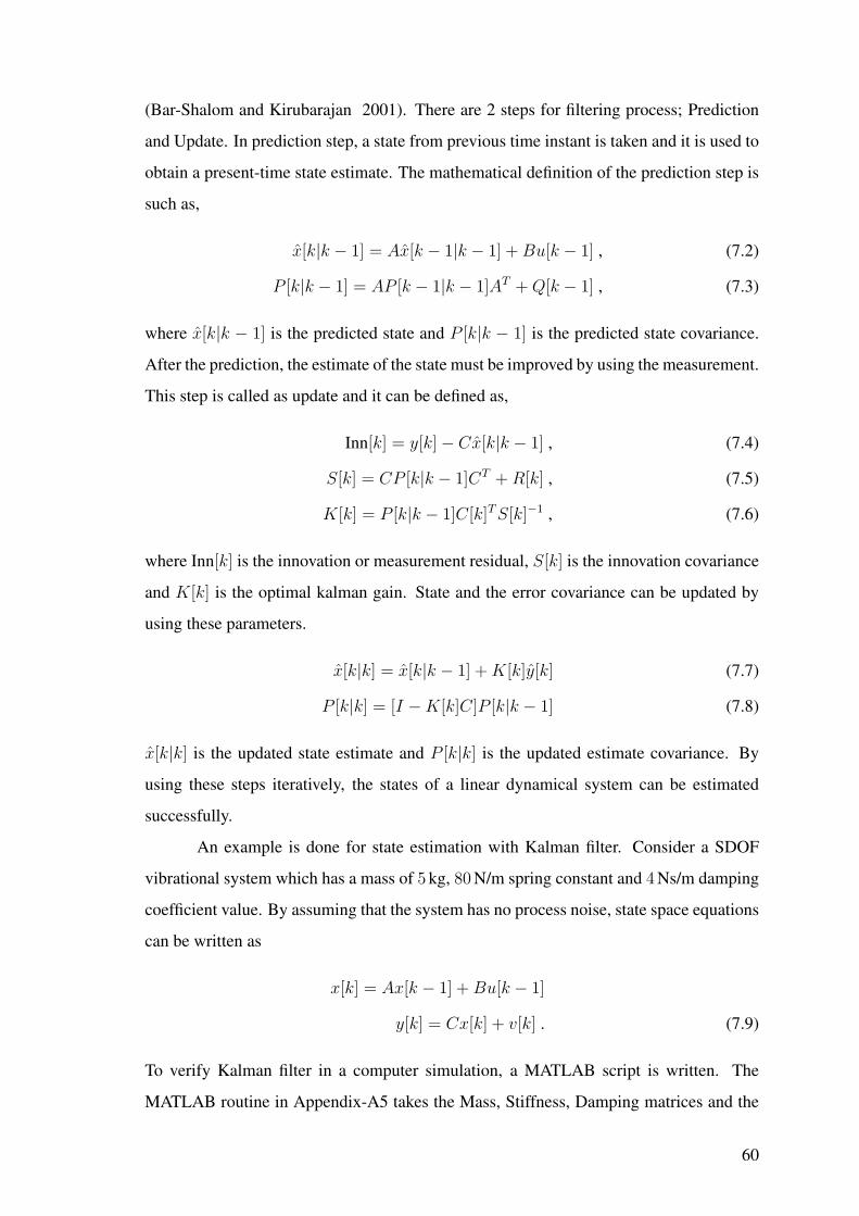
(Bar-Shalom and Kirubarajan 2001). There are 2 steps for filtering process; Prediction
and Update. In prediction step, a state from previous time instant is taken and it is used to
obtain a present-time state estimate. The mathematical definition of the prediction step is
such as,
x[k|k − 1] = Ax[k − 1|k − 1] + Bu[k − 1] , (7.2)
P [k|k − 1] = AP [k − 1|k − 1]AT + Q[k − 1] , (7.3)
where x[k|k − 1] is the predicted state and P [k|k − 1] is the predicted state covariance.
After the prediction, the estimate of the state must be improved by using the measurement.
This step is called as update and it can be defined as,
Inn[k] = y[k]− Cx[k|k − 1] , (7.4)
S[k] = CP [k|k − 1]CT + R[k] , (7.5)
K[k] = P [k|k − 1]C[k]T S[k]−1 , (7.6)
where Inn[k] is the innovation or measurement residual, S[k] is the innovation covariance
and K[k] is the optimal kalman gain. State and the error covariance can be updated by
using these parameters.
x[k|k] = x[k|k − 1] + K[k]y[k] (7.7)
P [k|k] = [I −K[k]C]P [k|k − 1] (7.8)
x[k|k] is the updated state estimate and P [k|k] is the updated estimate covariance. By
using these steps iteratively, the states of a linear dynamical system can be estimated
successfully.
An example is done for state estimation with Kalman filter. Consider a SDOF
vibrational system which has a mass of 5 kg, 80 N/m spring constant and 4 Ns/m damping
coefficient value. By assuming that the system has no process noise, state space equations
can be written as
x[k] = Ax[k − 1] + Bu[k − 1]
y[k] = Cx[k] + v[k] . (7.9)
To verify Kalman filter in a computer simulation, a MATLAB script is written. The
MATLAB routine in Appendix-A5 takes the Mass, Stiffness, Damping matrices and the
60
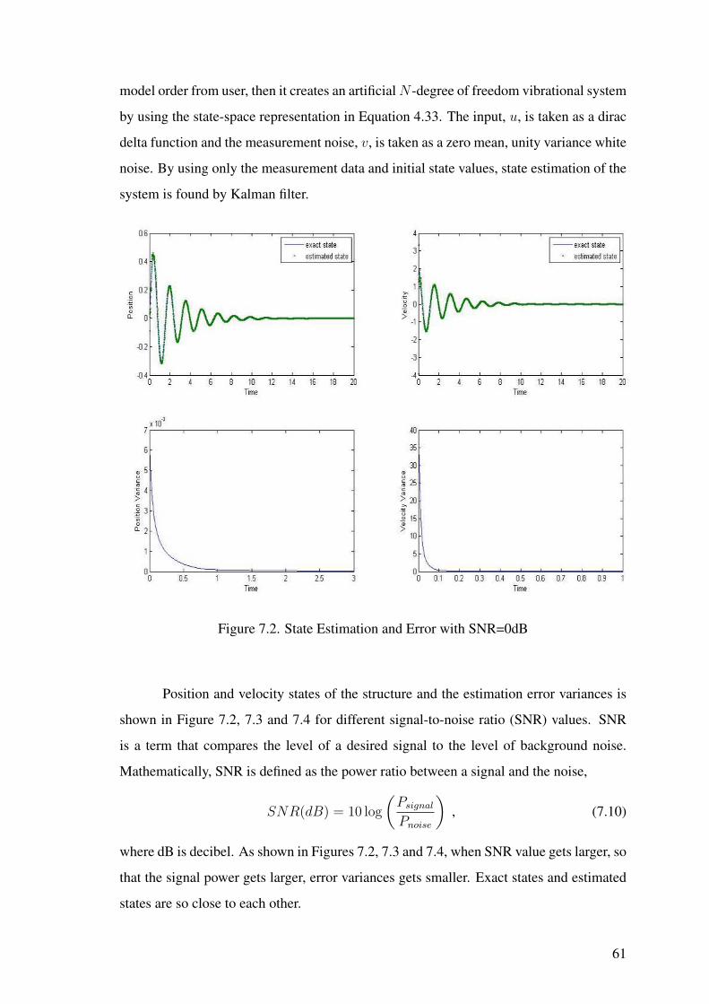
model order from user, then it creates an artificial N -degree of freedom vibrational system
by using the state-space representation in Equation 4.33. The input, u, is taken as a dirac
delta function and the measurement noise, v, is taken as a zero mean, unity variance white
noise. By using only the measurement data and initial state values, state estimation of the
system is found by Kalman filter.
Figure 7.2. State Estimation and Error with SNR=0dB
Position and velocity states of the structure and the estimation error variances is
shown in Figure 7.2, 7.3 and 7.4 for different signal-to-noise ratio (SNR) values. SNR
is a term that compares the level of a desired signal to the level of background noise.
Mathematically, SNR is defined as the power ratio between a signal and the noise,
SNR(dB) = 10 log
(Psignal
Pnoise
), (7.10)
where dB is decibel. As shown in Figures 7.2, 7.3 and 7.4, when SNR value gets larger, so
that the signal power gets larger, error variances gets smaller. Exact states and estimated
states are so close to each other.
61
Figure 7.3. State Estimation and Error with SNR=20dB
As comparison graphs of the estimated states and exact states, consistency of the
filter is also important. Consistency of a filter is the convergence of the estimate to the
true value. Consistency in the mean square sense can be defined as,
limk→∞
E[[x(k, Y k)− x0]2] = 0 . (7.11)
To decide the consistency of our filter, we made a statistical test. The error function is
taken as,
ε(k) = x[k|k]T P [k|k]−1x[k|k], x[k|k] = x[k|k]− x[k|k] . (7.12)
ε(k) is also called Normalized State Estimation Error Squared (NEES) and this variable
can be taken as a chi-square random variable. Chi-square Distribution is defined as
ε ∼ χ2nx→ ε =
k∑i=1
x2i , (7.13)
where xi’s are k independent, normally distributed random variables with mean 0 and
62
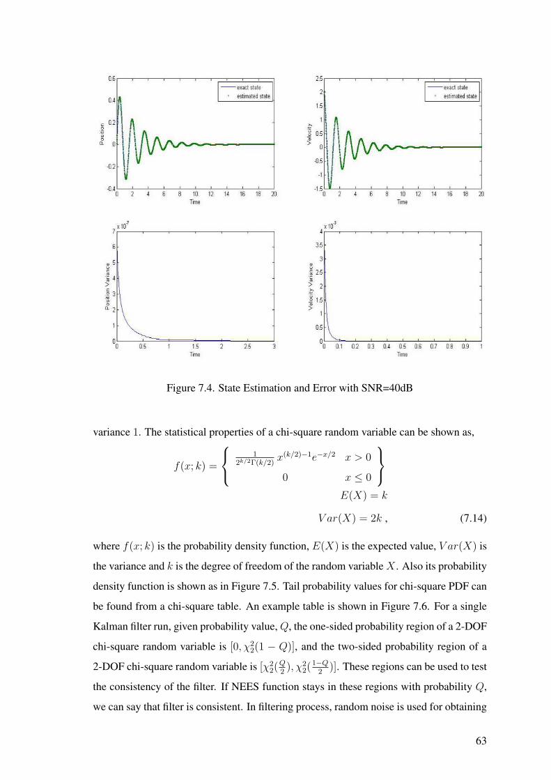
Figure 7.4. State Estimation and Error with SNR=40dB
variance 1. The statistical properties of a chi-square random variable can be shown as,
f(x; k) =
12k/2Γ(k/2)
x(k/2)−1e−x/2 x > 0
0 x ≤ 0
E(X) = k
V ar(X) = 2k , (7.14)
where f(x; k) is the probability density function, E(X) is the expected value, V ar(X) is
the variance and k is the degree of freedom of the random variable X . Also its probability
density function is shown as in Figure 7.5. Tail probability values for chi-square PDF can
be found from a chi-square table. An example table is shown in Figure 7.6. For a single
Kalman filter run, given probability value, Q, the one-sided probability region of a 2-DOF
chi-square random variable is [0, χ22(1 − Q)], and the two-sided probability region of a
2-DOF chi-square random variable is [χ22(
Q2), χ2
2(1−Q
2)]. These regions can be used to test
the consistency of the filter. If NEES function stays in these regions with probability Q,
we can say that filter is consistent. In filtering process, random noise is used for obtaining
63
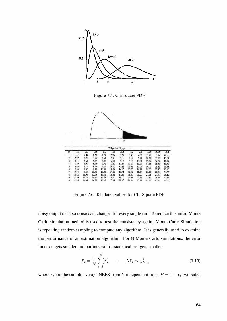
Figure 7.5. Chi-square PDF
Figure 7.6. Tabulated values for Chi-Square PDF
noisy output data, so noise data changes for every single run. To reduce this error, Monte
Carlo simulation method is used to test the consistency again. Monte Carlo Simulation
is repeating random sampling to compute any algorithm. It is generally used to examine
the performance of an estimation algorithm. For N Monte Carlo simulations, the error
function gets smaller and our interval for statistical test gets smaller.
εx =1
N
N∑i=1
εix → Nεx ∼ χ2
Nnx(7.15)
where εx are the sample average NEES from N independent runs. P = 1 − Q two-sided
64
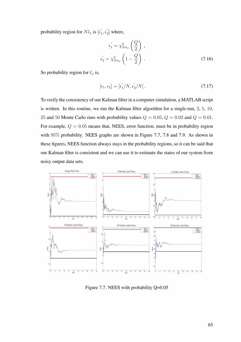
probability region for Nεx is [ε′1, ε
′2] where,
ε′1 = χ2
Nnx
(Q
2
),
ε′2 = χ2
Nnx
(1− Q
2
). (7.16)
So probability region for εx is,
[ε1, ε2] = [ε′1/N, ε
′2/N ] . (7.17)
To verify the consistency of our Kalman filter in a computer simulation, a MATLAB script
is written. In this routine, we run the Kalman filter algorithm for a single-run, 2, 5, 10,
25 and 50 Monte Carlo runs with probability values Q = 0.05, Q = 0.02 and Q = 0.01.
For example, Q = 0.05 means that, NEES, error function, must be in probability region
with 95% probability. NEES graphs are shown in Figure 7.7, 7.8 and 7.9. As shown in
these figures, NEES function always stays in the probability regions, so it can be said that
our Kalman filter is consistent and we can use it to estimate the states of our system from
noisy output data sets.
Figure 7.7. NEES with probability Q=0.05
65
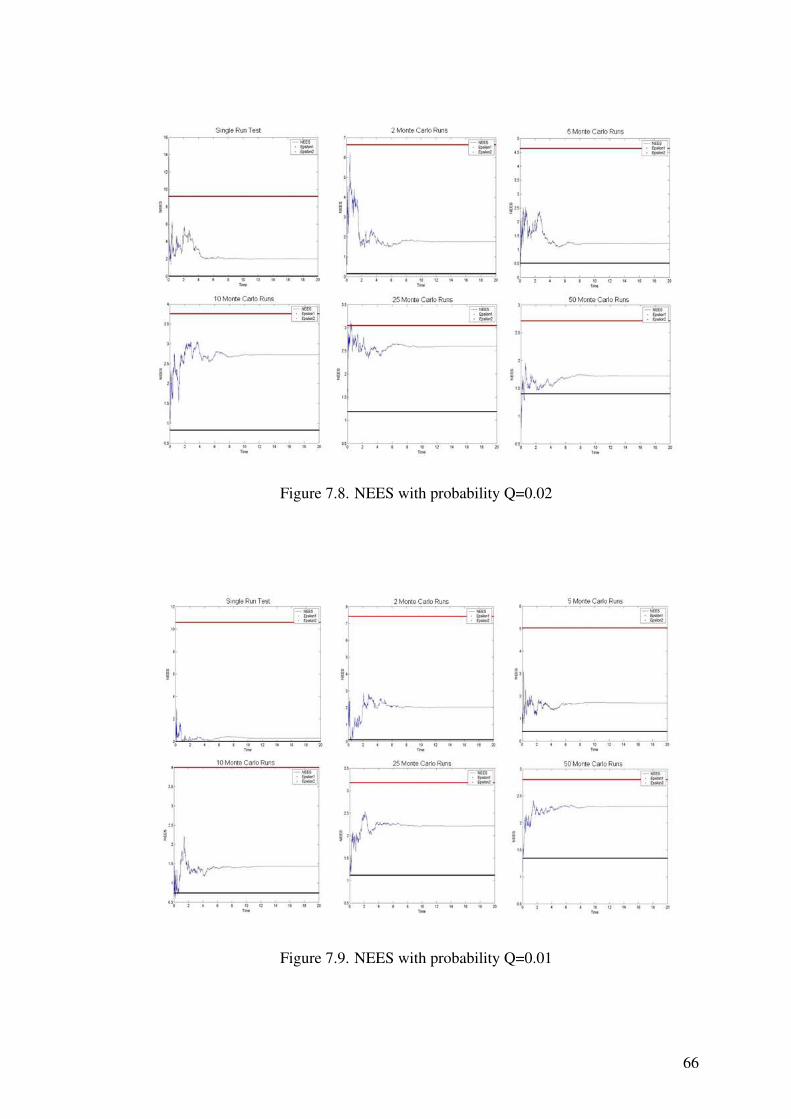
Figure 7.8. NEES with probability Q=0.02
Figure 7.9. NEES with probability Q=0.01
66
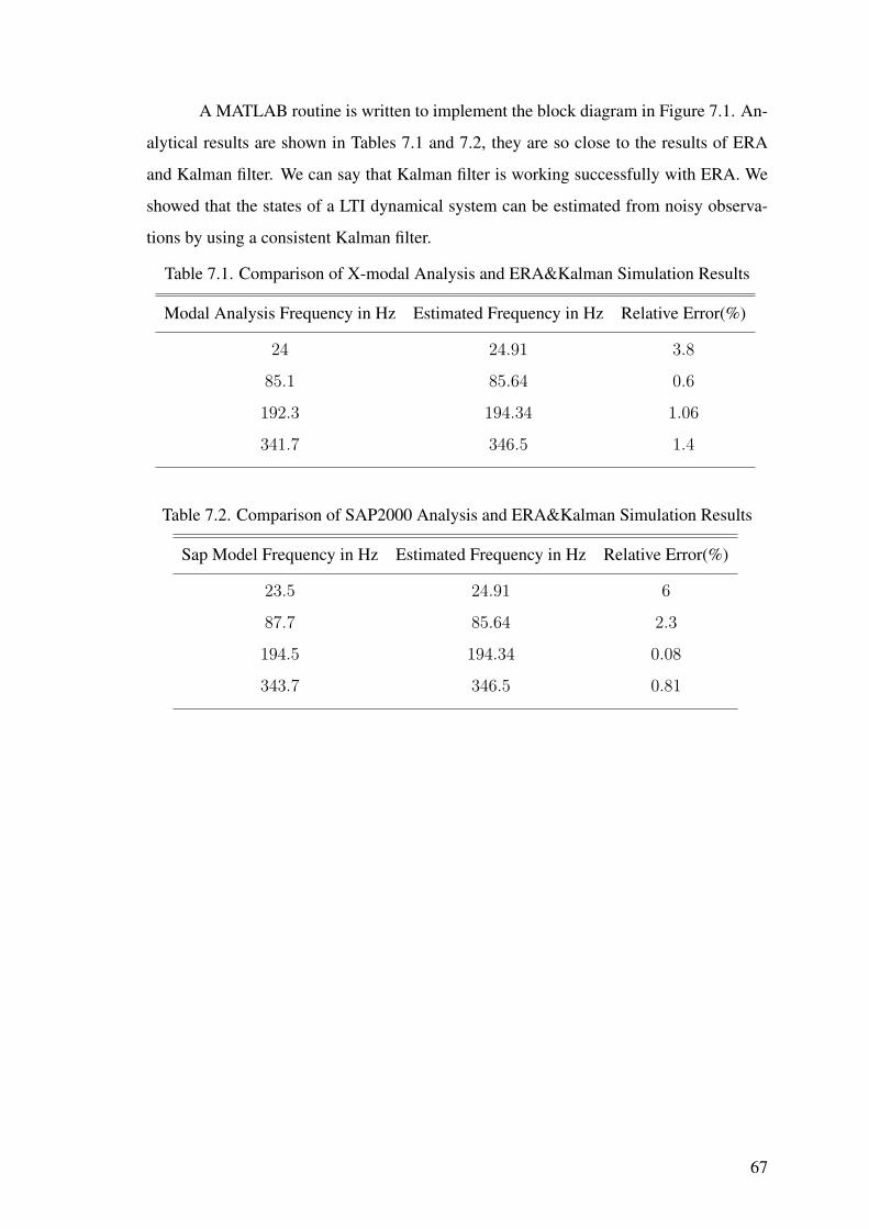
A MATLAB routine is written to implement the block diagram in Figure 7.1. An-
alytical results are shown in Tables 7.1 and 7.2, they are so close to the results of ERA
and Kalman filter. We can say that Kalman filter is working successfully with ERA. We
showed that the states of a LTI dynamical system can be estimated from noisy observa-
tions by using a consistent Kalman filter.
Table 7.1. Comparison of X-modal Analysis and ERA&Kalman Simulation Results
Modal Analysis Frequency in Hz Estimated Frequency in Hz Relative Error(%)
24 24.91 3.8
85.1 85.64 0.6
192.3 194.34 1.06
341.7 346.5 1.4
Table 7.2. Comparison of SAP2000 Analysis and ERA&Kalman Simulation Results
Sap Model Frequency in Hz Estimated Frequency in Hz Relative Error(%)
23.5 24.91 6
87.7 85.64 2.3
194.5 194.34 0.08
343.7 346.5 0.81
67
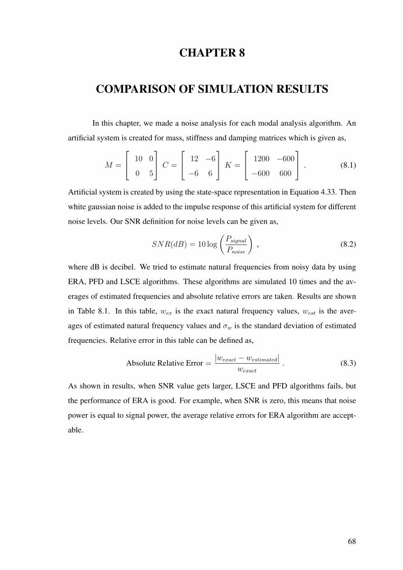
CHAPTER 8
COMPARISON OF SIMULATION RESULTS
In this chapter, we made a noise analysis for each modal analysis algorithm. An
artificial system is created for mass, stiffness and damping matrices which is given as,
M =
10 0
0 5
C =
12 −6
−6 6
K =
1200 −600
−600 600
. (8.1)
Artificial system is created by using the state-space representation in Equation 4.33. Then
white gaussian noise is added to the impulse response of this artificial system for different
noise levels. Our SNR definition for noise levels can be given as,
SNR(dB) = 10 log
(Psignal
Pnoise
), (8.2)
where dB is decibel. We tried to estimate natural frequencies from noisy data by using
ERA, PFD and LSCE algorithms. These algorithms are simulated 10 times and the av-
erages of estimated frequencies and absolute relative errors are taken. Results are shown
in Table 8.1. In this table, wex is the exact natural frequency values, west is the aver-
ages of estimated natural frequency values and σw is the standard deviation of estimated
frequencies. Relative error in this table can be defined as,
Absolute Relative Error =|wexact − westimated|
wexact
. (8.3)
As shown in results, when SNR value gets larger, LSCE and PFD algorithms fails, but
the performance of ERA is good. For example, when SNR is zero, this means that noise
power is equal to signal power, the average relative errors for ERA algorithm are accept-
able.
68

Table 8.1. Comparison of Modal Analysis Algorithms for Different Noise Levels
Algorithm SNR wex west σw Average Absolute Relative Error
(dB) (rad/s) (rad/s) (%)
80 14.31 14.36 0.0416 0.37
80 5.93 6.04 0.1073 1.92
60 14.31 14.27 0.004 0.28
60 5.93 0.78 0.0532 86.2
LSCE 40 14.31 14.32 0.0254 0.17
40 5.93 31.32 4.4171 422.32
20 14.31 212.52 26.48 1384.9
20 5.93 12.60 0.0869 112.68
50 14.31 14.30 0.0243 0.14
50 5.93 5.92 0.0138 0.21
PFD 30 14.31 13.24 0.3084 7.4
30 5.93 5.12 0.1930 13.5
10 14.31 0.78 0.6163 94.53
10 5.93 0.49 0.2753 91.72
10 14.31 14.25 0.0143 0.18
ERA 10 5.93 5.93 0.1483 0.89
0 14.31 14.45 0.0430 0.6
0 5.93 5.91 0.5571 3.2
69
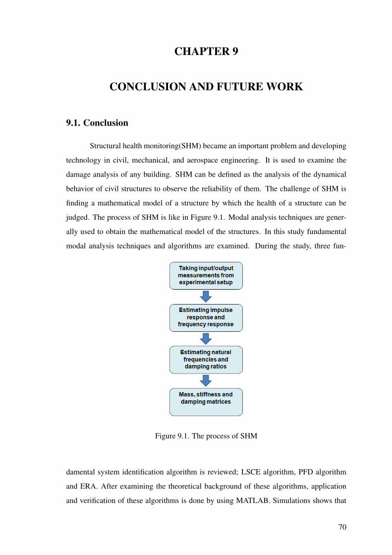
CHAPTER 9
CONCLUSION AND FUTURE WORK
9.1. Conclusion
Structural health monitoring(SHM) became an important problem and developing
technology in civil, mechanical, and aerospace engineering. It is used to examine the
damage analysis of any building. SHM can be defined as the analysis of the dynamical
behavior of civil structures to observe the reliability of them. The challenge of SHM is
finding a mathematical model of a structure by which the health of a structure can be
judged. The process of SHM is like in Figure 9.1. Modal analysis techniques are gener-
ally used to obtain the mathematical model of the structures. In this study fundamental
modal analysis techniques and algorithms are examined. During the study, three fun-
Figure 9.1. The process of SHM
damental system identification algorithm is reviewed; LSCE algorithm, PFD algorithm
and ERA. After examining the theoretical background of these algorithms, application
and verification of these algorithms is done by using MATLAB. Simulations shows that
70
the parameters of a structure can be identified correctly from clear measurements. The
response of artificial 1-DOF and 2-DOF systems are used in MATLAB simulations to
verify the methods.
Although the verification of the PFD method for artificial models is implemented
successfully, the parameters of experimental system can not be identified from experi-
mental measurements because of the measurement noise. PFD algorithm is so sensitive
to noise. Also performance of LSCE is good when there isn’t noise in measurement, but
when noise is present in the data, this method performs poorly.
ERA incorporates singular value decomposition to counteract inherent noise and
it gives satisfactory results for the experimental measurement data. We can say that ERA
is a more robust algorithm than LSCE or PFD. We used ERA and Kalman filter together
to update the system parameters and we have found good results.
9.2. Future Work
Since EM is an efficient algorithm for communication systems, it can be used for
linear dynamical systems as vibrational systems. To use EM for vibrational systems, the
states of the system must be estimated. Kalman filter estimates the state of a dynamical
system from a series of incomplete and noisy measurements. By using the estimated
state at each time instant, the parameters of the system can be estimated by using EM
algorithm.
Because of the measurement noise and the nonlinearity of the structures, a new
advanced method for identification of a structure can be established. The basis of this
new method will be upon the variants of Kalman filter and EM algorithm. To set up this
new method successfully, we need an initial estimate of system parameters. We can use
the result of the ERA algorithm as an initial guess of parameters and try to estimate the
real parameters iteratively by using EM algorithm. Also Extended Kalman filter can be
used with EM algorithm for nonlinear models. This will be a new solution approach for
SHM problem. Now an introductory knowledge about EM algorithm will be given.
The main objective of EM algorithm is to build a probabilistic model of a real-life
structure which can be defined by some parameters. By using EM algorithm, the noise in
observation data can be eliminated during the identification procedure, so the identified
system parameters becomes more realistic, this is the advantage of the EM. To understand
71
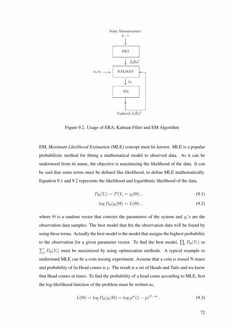
Figure 9.2. Usage of ERA, Kalman Filter and EM Algorithm
EM, Maximum Likelihood Estimation (MLE) concept must be known. MLE is a popular
probabilistic method for fitting a mathematical model to observed data. As it can be
understood from its name, the objective is maximizing the likelihood of the data. It can
be said that some terms must be defined like likelihood, to define MLE mathematically.
Equation 9.1 and 9.2 represents the likelihood and logarithmic likelihood of the data,
PΘ(Yi) = P (Yi = yi|Θ) , (9.1)
log PΘ(yi|Θ) = L(Θ) , (9.2)
where Θ is a random vector that consists the parameters of the system and yi’s are the
observation data samples. The best model that fits the observation data will be found by
using these terms. Actually the best model is the model that assigns the highest probability
to the observation for a given parameter vector. To find the best model,∏
i PΘ(Yi) or∑
i PΘ(Yi) must be maximized by using optimization methods. A typical example to
understand MLE can be a coin tossing experiment. Assume that a coin is tossed N times
and probability of oa Head comes is p. The result is a set of Heads and Tails and we know
that Head comes m times. To find the probability of a head come according to MLE, first
the log-likelihood function of the problem must be written as,
L(Θ) = log PΘ(yi|Θ) = log pm(1− p)N−m . (9.3)
72
Then log-likelihood function must be maximized. By taking the derivative of the Equation
9.3 and equalize it to zero, parameter p can be found.
dL(Θ)
dΘ=
m
p− N −m
1− p= 0 (9.4)
p =m
N(9.5)
In this example problem, there was no unobserved data or any noisy measurement, MLE
worked successfully for this case, but what happens if any unobserved data or noisy mea-
surement data set occurs. The answer is an intuitive and iterative algorithm, EM. There
are 3 steps for EM algorithm;
⇒ Create an initial parameter vector Θ0
⇒ Use Θ0 to obtain new model , with Θ1, that provides L(Θ1) > L(Θ0)
⇒ Obtain a sequence like L(Θ0) < L(Θ1) < .... < L(ΘN)
ΘN is the parameter vector of our system and we can define the mathematical model of
the structure by using it. For example Θ can be defined as [A,B, C]T for the system in
Equation 7.3. If the states that are estimated from Kalman filter used together with EM
algorithm, it can be possible that the parameters of the state-space system in Equation 7.3
can be estimated iteratively.
As shown in Figure 9.2, theoretical underwork of this method is ready but it must
be verified by a computer simulation. We run the ERA and Kalman filter together, but we
haven’t used the EM algorithm yet. The simulation of EM algorithm is left as a future
work for this study.
73
REFERENCES
Isaac, Newton. 1687. Philosophiae Naturalis Principia Mathematica.
I.B. Cohen and A. Whitman. 1999. The Principia : A new translation. University ofCalifornia press, Berkeley.
A.C. Ugural and S.K. Fenster. 2003. Advanced Strength and Applied Elasticity. New Jer-sey: Prentice Hall.
Chopra, Anil K. 1995. Dynamics of Structures, Theory and Applications to EarthquakeEngineering. New Jersey: Prentice Hall.
Ogata, Katsuhiko. 1995. System Dynamics. New Jersey: Prentice Hall.
Allemang, Randall. 1999. Vibrations: Analytical and Experimental Modal Analysis.
Jimin He and Zhi-Fang Fu. 2001. Modal Analysis. Oxford: Butterworth-Heinemann.
Eyyub Karakan. 2008. Estimation of Frequency Response Function for ExperimentalModal Analysis. Department of Civil Engineering. Izmir Institute of Technology.
Zhang, L. and H. Kanda. 1985. A Polyreference Frequency Domain Method for ModalParameter Identification. Mechanical Systems and Signal Processing Volume 4,Issue 1, p. 65-75.
F. Lembregts and J. Leuridan. 1990. Frequency Domain Direct Parameter Identificationfor Modal Analysis: State Space Formulation. ASME Design Engineering Con-ference, Cincinnati, Ohio.
Ho B.L. and Kalman R.E. 1963. Effective Construction of Linear State Variable Modelsfrom Input/Output Data. Regelungstechnik 14 545-548.
Juang J.N. and Pappa R.S. 1985. An eigensystem realization algorithm for modal param-eter identification and model reduction. J. Guidance, Control and Dynamics 9(3):294-303.
Juang J.N. and Cooper J.E. 1987. An Eigensystem Realization Algorithm Using DataCorrelations For Modal Parameter Identification. J. Guidance, Control and Dy-namics 9(3): 294-303.
Pappa R.S. and Elliott K.B. 1992. A Consistent Mode Indicator For The EigensystemRealization Algorithm NASA Technical Memorandum 107607.
Marlon D. Hill. 2003. An Experimental Verification of the Eigensystem Realization Al-gorithm For Vibration Parameter Identification Florida A&M University.
Yaakov Bar-Shalom and Thiagalingam Kirubarajan, eds. 2001. Estimation with Applica-tions to Tracking and Navigation. John Wiley & Sons Inc.
Scharf, Louis L. 2001. Statistical Signal Processing. Addison-Wesley.
74

Todd K. Moon and Wynn C. Stirling. 2000. Mathematical Methods and Algorithms forSignal Processing.
Ninness B. and Gibson S. 1987. The EM Algorithm for Multivariable Dynamic SystemEstimation. J. Guidance, Control and Dynamics 9(3): 294-303.
75
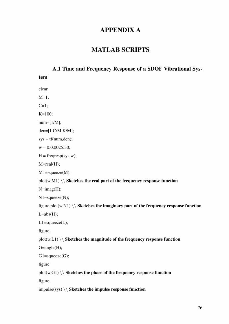
APPENDIX A
MATLAB SCRIPTS
A.1 Time and Frequency Response of a SDOF Vibrational Sys-tem
clear
M=1;
C=1;
K=100;
num=[1/M];
den=[1 C/M K/M];
sys = tf(num,den);
w = 0:0.0025:30;
H = freqresp(sys,w);
M=real(H);
M1=squeeze(M);
plot(w,M1) \\ Sketches the real part of the frequency response function
N=imag(H);
N1=squeeze(N);
figure plot(w,N1) \\ Sketches the imaginary part of the frequency response function
L=abs(H);
L1=squeeze(L);
figure
plot(w,L1) \\ Sketches the magnitude of the frequency response function
G=angle(H);
G1=squeeze(G);
figure
plot(w,G1) \\ Sketches the phase of the frequency response function
figure
impulse(sys) \\ Sketches the impulse response function
76
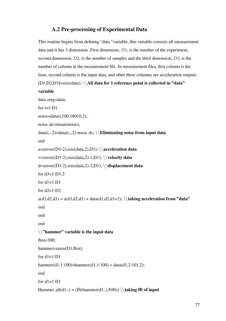
A.2 Pre-processing of Experimental Data
This routine begins from defining “data ”variable, this variable consists all measurement
data and it has 3 dimension. First dimension, D1, is the number of the experiment,
second dimension, D2, is the number of samples and the third dimension, D3, is the
number of column in the measurement file. In measurement files, first column is the
time, second column is the input data, and other three columns are acceleration outputs.
[D1,D2,D3]=size(data); \\All data for 1 reference point is collected in ”data”
variable
data orig=data;
for i=1:D1
noise=data(i,100:18010,2);
noise dc=mean(noise);
data(i,:,2)=data(i,:,2)-noise dc; \\Eliminating noise from input data
end
a=zeros((D3-2),size(data,2),D1); \\acceleration data
v=zeros((D3-2),size(data,2)-1,D1); \\velocity data
d=zeros((D3-2),size(data,2)-2,D1); \\displacement data
for d3=1:D3-2
for d1=1:D1
for d2=1:D2
a(d3,d2,d1) = a(d3,d2,d1) + data(d1,d2,d3+2); \\taking acceleration from ”data”
end
end
end
\\”hammer” variable is the input data
flen=300;
hammer=zeros(D1,flen);
for d1=1:D1
hammer(d1,1:100)=hammer(d1,1:100) + data(d1,2:101,2);
end
for d1=1:D1
Hammer all(d1,:) = (fft(hammer(d1,:),Nfft)) \\taking fft of input
77
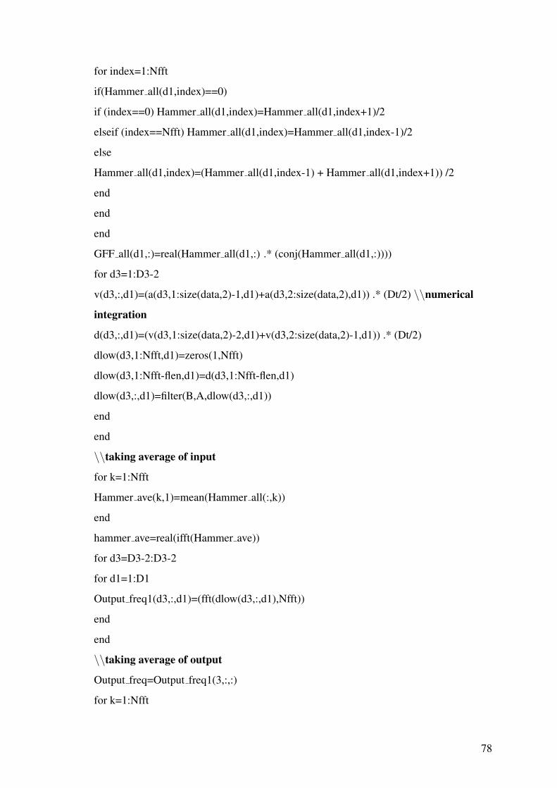
for index=1:Nfft
if(Hammer all(d1,index)==0)
if (index==0) Hammer all(d1,index)=Hammer all(d1,index+1)/2
elseif (index==Nfft) Hammer all(d1,index)=Hammer all(d1,index-1)/2
else
Hammer all(d1,index)=(Hammer all(d1,index-1) + Hammer all(d1,index+1)) /2
end
end
end
GFF all(d1,:)=real(Hammer all(d1,:) .* (conj(Hammer all(d1,:))))
for d3=1:D3-2
v(d3,:,d1)=(a(d3,1:size(data,2)-1,d1)+a(d3,2:size(data,2),d1)) .* (Dt/2) \\numerical
integration
d(d3,:,d1)=(v(d3,1:size(data,2)-2,d1)+v(d3,2:size(data,2)-1,d1)) .* (Dt/2)
dlow(d3,1:Nfft,d1)=zeros(1,Nfft)
dlow(d3,1:Nfft-flen,d1)=d(d3,1:Nfft-flen,d1)
dlow(d3,:,d1)=filter(B,A,dlow(d3,:,d1))
end
end
\\taking average of input
for k=1:Nfft
Hammer ave(k,1)=mean(Hammer all(:,k))
end
hammer ave=real(ifft(Hammer ave))
for d3=D3-2:D3-2
for d1=1:D1
Output freq1(d3,:,d1)=(fft(dlow(d3,:,d1),Nfft))
end
end
\\taking average of output
Output freq=Output freq1(3,:,:)
for k=1:Nfft
78
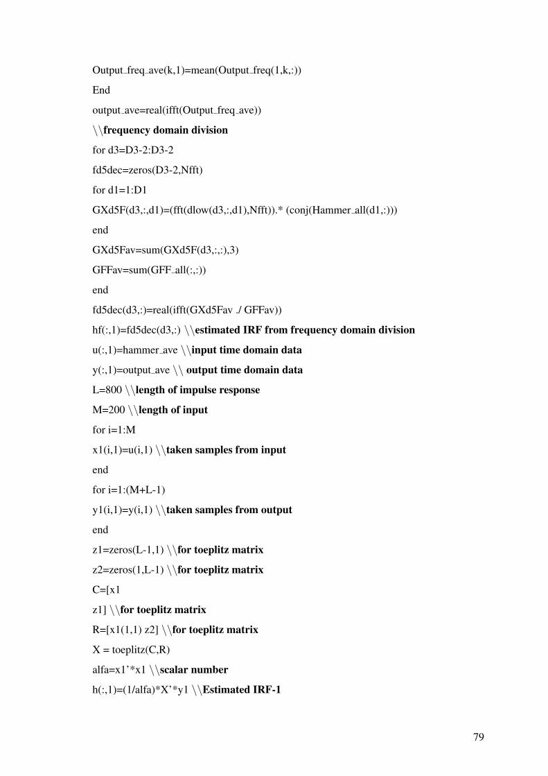
Output freq ave(k,1)=mean(Output freq(1,k,:))
End
output ave=real(ifft(Output freq ave))
\\frequency domain division
for d3=D3-2:D3-2
fd5dec=zeros(D3-2,Nfft)
for d1=1:D1
GXd5F(d3,:,d1)=(fft(dlow(d3,:,d1),Nfft)).* (conj(Hammer all(d1,:)))
end
GXd5Fav=sum(GXd5F(d3,:,:),3)
GFFav=sum(GFF all(:,:))
end
fd5dec(d3,:)=real(ifft(GXd5Fav ./ GFFav))
hf(:,1)=fd5dec(d3,:) \\estimated IRF from frequency domain division
u(:,1)=hammer ave \\input time domain data
y(:,1)=output ave \\ output time domain data
L=800 \\length of impulse response
M=200 \\length of input
for i=1:M
x1(i,1)=u(i,1) \\taken samples from input
end
for i=1:(M+L-1)
y1(i,1)=y(i,1) \\taken samples from output
end
z1=zeros(L-1,1) \\for toeplitz matrix
z2=zeros(1,L-1) \\for toeplitz matrix
C=[x1
z1] \\for toeplitz matrix
R=[x1(1,1) z2] \\for toeplitz matrix
X = toeplitz(C,R)
alfa=x1’*x1 \\scalar number
h(:,1)=(1/alfa)*X’*y1 \\Estimated IRF-1
79

h1(:,1)=inv(X’*X)*X’*y1 \\Estimated IRF-2
end
80
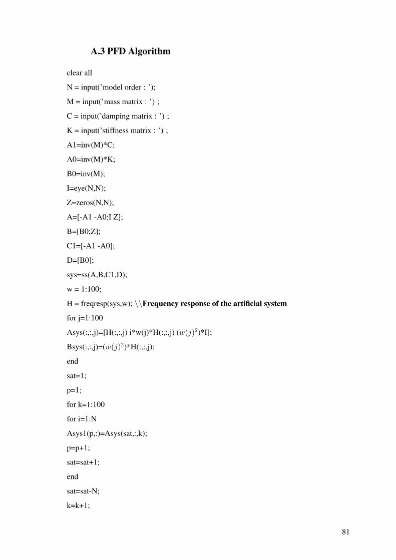
A.3 PFD Algorithm
clear all
N = input(’model order : ’);
M = input(’mass matrix : ’) ;
C = input(’damping matrix : ’) ;
K = input(’stiffness matrix : ’) ;
A1=inv(M)*C;
A0=inv(M)*K;
B0=inv(M);
I=eye(N,N);
Z=zeros(N,N);
A=[-A1 -A0;I Z];
B=[B0;Z];
C1=[-A1 -A0];
D=[B0];
sys=ss(A,B,C1,D);
w = 1:100;
H = freqresp(sys,w); \\Frequency response of the artificial system
for j=1:100
Asys(:,:,j)=[H(:,:,j) i*w(j)*H(:,:,j) (w(j)2)*I];
Bsys(:,:,j)=(w(j)2)*H(:,:,j);
end
sat=1;
p=1;
for k=1:100
for i=1:N
Asys1(p,:)=Asys(sat,:,k);
p=p+1;
sat=sat+1;
end
sat=sat-N;
k=k+1;
81
end
sat=1;
p=1;
for k=1:100
for i=1:N
Bsys1(p,:)=Bsys(sat,:,k);
p=p+1;
sat=sat+1;
end
sat=sat-N;
k=k+1;
end
[Q,R] = qr(Asys1);
x=pinv(R)*(Q’)*Bsys1 \\ estimated A1, A0 and B0 matrices
for n=1:N
A12(n,:)=[x(n,:)]; \\estimated A0 matrix
end
f=1;
for n=(N+1):(N2)
A11(f,:)=[x(n,:)]; \\estimated A1 matrix
f=f+1;
end
A111=[-A11 -A12;I Z]; \\ estimated A matrix
roots=eig(A111); \\estimated roots
for n1=1:N
estfreq(n1)=imag(roots(n1)); \\estimated natural frequency
estdamp(n1)=-real(roots(n1))/estfreq(n1); \\estimated damping ratio
end
82

A.4 LSCE Algorithm for Artificial Data
clear all
N = input(’model order : ’);
M = input(’mass matrix : ’) ;
C = input(’damping matrix : ’) ;
K = input(’stiffness matrix : ’) ;
A1=inv(M)*C;
A0=inv(M)*K;
B0=inv(M);
I=eye(N,N);
Z=zeros(N,N);
A=[-A1 -A0;I Z];
B=[B0;Z];
C1=[-A1 -A0];
D=[B0];
sys=ss(A,B,C1,D);
Fs =20; \\ Sampling Frequency
Dt=1/Fs;
T=250; \\ Duration of the signal
t=0:Dt:T; \\ Time interval
y=impulse(sys,t); \\ Impulse response functions of the system
num=Fs*T+1; \\ Number of samples
\\ Maps the impulse responses to variables h11,h12,h21,h22..
for k=1:N
for l=1:N
for j=1:num
eval(sprintf(’h1%d%d(j,1)=y(j,k,l);’,k,l));
end
eval(sprintf(’h%d%d=h1%d%d”;’,k,l,k,l));
end
end
r0=50; \\ Reading offset
83
L=N*2; \\ Number of samples to be used for cosntructing the Hankel matrix
odet=4; \\ Overdetermine factor
for k=1:N
for l=1:N
eval(sprintf(’Y%d%d = hankel(h%d%d(r0+1:r0+L*odet)”,
h%d%d(r0+L*odet:r0+L*odet+N*2-1));’,k,l,k,l,k,l)); \\ Hankel matrix
eval(sprintf(’x%d%d=[h%d%d(r0+N*2+1:r0+L+L*odet)]”;’,k,l,k,l));
eval(sprintf(’betavec%d%d = inv(Y %d %d”*Y %d %d)*Y %d %d”*x %d
%d;’,k,l,k,l,k,l,k,l,k,l)); \\ Beta vector
eval(sprintf(’rootspoly %d%d = roots(flipud([betavec % d % d ; -1]));’,k,l,k,l));
eval(sprintf(’w%d%d =
Fs*(sqrt(log(rootspoly%d%d).*log(conj(rootspoly%d%d))));’,k,l,k,l,k,l)); \\ Identified
natural frequencies for h11,h12...
end
end
\\ Following routine calculates the real natural frequencies from M, C, K matrices
syms w
A=det(K-w2*M);
Realfreq=eval(solve(A));
n=1;
for i=1:(N*2)
if Realfreq(i)>0
W(n,:)=Realfreq(i);
n=n+1;
end
end
W
84

A.5 LSCE Algorithm for Experimental Data
[N,nout]=size(data); \\ size of impulse response data
m=1; \\ number of output
len=min(ceil(N/5),205);
xlen=len;
nrow=floor((N-m)/len)*(len/xlen)-2;
\\ constructing Hankel matrix
datat=data’;
for i=1:(nrow)
H0((i-1)*nout+1:i*nout,1:len)=datat(1:nout,(i-1)*xlen+1:(i-1)*xlen+len);
X0((i-1)*nout+1:i*nout,1)=datat(1:nout,i*len+1);
end
beta vec = inv(H0’*H0)*H0’*X0; \\ beta vector for prony polynomial
roots poly = roots(flipud([beta vec ; -1])); \\ roots of polynomial
Fs=1/deltat; \\ sampling frequency
w = Fs*(sqrt(log(roots poly).*log(conj(roots poly)))); \\ Natural Frequencies
ksi = -log(roots poly.*conj(roots poly))*Fs/(2*w); \\ Damping ratio values
85
A.6 ERA Algorithm for Artificial Data
clear all
N = input(’model order : ’);
M = input(’mass matrix : ’) ;
C = input(’damping matrix : ’) ;
K = input(’stiffness matrix : ’) ;
A1=inv(M)*C;
A0=inv(M)*K;
B0=inv(M);
I=eye(N,N);
Z=zeros(N,N);
A=[-A1 -A0;I Z];
B=[B0;Z];
C1=[-A1 -A0];
D=[B0];
sys=ss(A,B,C1,D); \\defining the state-space model
Fs = 100; \\sampling frequency
Dt=1/Fs;
T=100; \\duration of the signal
t=0:Dt:T; \\time interval
y=impulse(sys,t); \\impulse response of the system
num=Fs*T+1; \\number of samples
for k=1:N
for l=1:N
for j=1:num
eval(sprintf(’h1end
eval(sprintf(’hend
end
r0=10; \\reading offset
L=100; \\number of samples to be used for cosntructing the Hankel matrix
H0 = hankel(h11(r0+1:r0+L)”, h11(r0+L:r0+L+N*2-1)); \\hankel matrix H0
H1 = hankel(h11(r0+2:r0+L+1)”, h11(r0+L+1:r0+L+N*2)); \\hankel matrix H1
86

order=rank(H0); \\order of the system
[Pmax,Dmax,Qmax] = svd(H0); \\singular value decomposition of Hankel matrix
P=Pmax(:,1:order); \\reducing order of P
D=Dmax(1:order,1:order); \\reducing order of D
Q=Qmax(:,1:order); \\reducing order of Q
A=[D( − 0.5)]*P’*H1*Q*[D( − 0.5)]; \\ state matrix of minimum order realization
z=eig(A); \\ eigenvalues of the system
a=1;
for i=1:2:order
omega(a)=imag(log(z(i))*Fs); \\estimated natural frequencies
dampratio(a)=-real(log(z(i))*Fs)/omega(a); \\ estimated damping ratios
a=a+1;
end
87
A.7 ERA Algorithm for Experimental Data
[N,nout]=size(data); \\ size of impulse response data
m=1; \\ number of output
len=min(ceil(N/10),205);
xlen=len;
nrow=floor((N-m)/len)*(len/xlen)-2;
\\ constructing Hankel matrix
datat=data’;
for i=1:nrow
H0((i-1)*nout+1:i*nout,1:len)=datat(1:nout,(i-1)*xlen+1:(i-1)*xlen+len);
H1((i-1)*nout+1:i*nout,1:len)=datat(1:nout,(i-1)*xlen+2:(i-1)*xlen+len+1);
end
dimH=size(H0);
[Plong,Dlong,Qlong]=svd(H0,’econ’); \\ singular value decomposition of Hankel
matrix
dimD=size(Dlong);
nfreqmax = min(50,dimD(2)/2);
nfreq=nfreqmax;
P=Plong(:,1:nfreqmax);
D=Dlong(1:nfreqmax,1:nfreqmax);
Q=Qlong(:,1:nfreqmax);
clear dimD;
dimD=size(D);
dimP=size(P);
dimQ=size(Q);
invrootD=zeros(dimD);
invrootD(1:nfreq,1:nfreq)=(D(1:nfreq,1:nfreq))(-0.5);
A=invrootD * P’ * H1 * Q * invrootD; \\ estimate of state matrix
(V, LAMBDA) = eig (A);
dimLAMBDA=size (LAMBDA);
LAMBDAv = LAMBDA * ones(dimLAMBDA(2),1);
for i=1:nfreq
88

if(abs(angle(LAMBDAv(i))) ¡ 1e-3) invrootD(i,i)=0; end
if(abs(abs(angle(LAMBDAv(i)))-pi) ¡ 1e-3) invrootD(i,i)=0; end
if(abs(LAMBDAv(i))¿1) invrootD(i,i)=0; end
end
Sv=(log(LAMBDAv))/deltat;
Lv=abs(log(LAMBDAv))/deltat;
zeta=-real(Sv(1:nfreq))./Lv(1:nfreq);
angular resonant freq=abs(imag(Sv(1:nfreq))./ sqrt(1 - zeta)); \\ frequency estimates
in rad/s
freq=(angular resonant freq angular resonant freq(2*pi)); \\ frequency estimates in
Hz
89
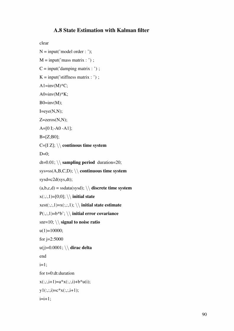
A.8 State Estimation with Kalman filter
clear
N = input(’model order : ’);
M = input(’mass matrix : ’) ;
C = input(’damping matrix : ’) ;
K = input(’stiffness matrix : ’) ;
A1=inv(M)*C;
A0=inv(M)*K;
B0=inv(M);
I=eye(N,N);
Z=zeros(N,N);
A=[0 I;-A0 -A1];
B=[Z;B0];
C=[I Z]; \\ continous time system
D=0;
dt=0.01; \\ sampling period duration=20;
sys=ss(A,B,C,D); \\ continuous time system
sysd=c2d(sys,dt);
(a,b,c,d) = ssdata(sysd); \\ discrete time system
x(:,:,1)=[0;0]; \\ initial state
xest(:,:,1)=x(:,:,1); \\ initial state estimate
P(:,:,1)=b*b’; \\ initial error covariance
snr=10; \\ signal to noise ratio
u(1)=10000;
for j=2:5000
u(j)=0.0001; \\ dirac delta
end
i=1;
for t=0:dt:duration
x(:,:,i+1)=a*x(:,:,i)+b*u(i);
y1(:,:,i)=c*x(:,:,i+1);
i=i+1;
90

end
y2=squeeze(y1);
y=awgn(y2,snr); \\ adding noise to observation
k=1;
Sz=0.1;
\\ Kalman Filter Equations
for t=0:dt:duration
xest(:,:,k+1)=a*xest(:,:,k)+b*u(k);
P(:,:,k+1)=a*P(:,:,k)*a’;
Inn=y(k)-c*xest(:,:,k);
S=c*P(:,:,k+1)*c’+Sz;
K=P(:,:,k+1)*c’*inv(S);
xest(:,:,k+1)=xest(:,:,k)+K*Inn;
P(:,:,k+1)=(I-K*c)*P(:,:,k+1);
k=k+1;
end
91