Embed Size (px)
Citation preview
IMA Journal of Numerical Analysis (2005) 25, 264–285doi:10.1093/imanum/drh016Advance Access publication 21 January 2005
Parameter estimation of ordinary differential equations
ZHENGFENG LI†National Centre for Epidemiology and Population Health, Australian National University,
Canberra, ACT 0200, Australia
MICHAEL R. OSBORNE‡School of Mathematical Sciences, Australian National University,
Canberra, ACT 0200, Australia
AND
TANIA PRVAN§
Department of Statistics, Macquarie University, Sydney, NSW 2109, Australia
[Received on 8 February 2002; revised on 5 January 2004]
This paper addresses the development of a new algorithm for parameter estimation of ordinary differentialequations. Here, we show that (1) the simultaneous approach combined with orthogonal cyclic reductioncan be used to reduce the estimation problem to an optimization problem subject to a fixed number ofequality constraints without the need for structural information to devise a stable embedding in the caseof non-trivial dichotomy and (2) the Newton approximation of the Hessian information of the Lagrangianfunction of the estimation problem should be used in cases where hypothesized models are incorrect oronly a limited amount of sample data is available. A new algorithm is proposed which includes the useof the sequential quadratic programming (SQP) Gauss–Newton approximation but also encompasses theSQP Newton approximation along with tests of when to use this approximation. This composite approachrelaxes the restrictions on the SQP Gauss–Newton approximation that the hypothesized model shouldbe correct and the sample data set large enough. This new algorithm has been tested on two standardproblems.
Keywords: ordinary differential equations; data fitting; parameter estimation; orthogonal cyclic reduction;constrained optimization; SQP methods; Gauss–Newton approximation.
1. Introduction
Assume that the ordinary differential equations (ODEs), after suitable normalization, have the form
dxdt
= f (t, x, θ), (1.1)
where t denotes the independent variable, usually referred to as time, θ is a p-dimensional vector ofunknown parameters, x = x(t, θ) is an n-dimensional state variable vector depending on t and θ, andthe function f (t, x, θ) maps �×�n ×�p into �n . In addition, side constraints are often given to specify
†Email: [email protected]‡Corresponding Author. Email: [email protected]§Email: [email protected]
IMA Journal of Numerical Analysis Vol. 25 No. 2 c© Institute of Mathematics and its Applications 2005; all rights reserved.
PARAMETER ESTIMATION OF ODES 265
further model properties such as boundary conditions, initial values or parameter restrictions
cp(x(t1), x(t f ), θ) = 0 ∈ Rq , (1.2)
where t1 is the initial time and t f is the final time.In order to estimate the unknown parameters, a number of measurements, say N , are available for
the process under consideration. These measurements often contain inherent errors and are characterizedby
yi = h(x(ti , θ)) + εi , i = 1, . . . , N , (1.3)
where yi ∈ �n is the measured value at ti , and {εi }Ni=1 are independently and identically normally
distributed errors. A common special case is that in which the state variables are observed directly, i.e.yi = x(ti , θ) + εi , i = 1, . . . , N . If the dynamical structure requires a dense grid, but only a fewexperimental times are available, one could insert dummy values with zero weights. Note that of theset of parameters making up the vector θ, some may enter only in f , others only in cp. The parameterestimation problem is to find reasonable values for θ so that the solution of the system (1.1)–(1.2) withthese values fits the given data {yi }N
i=1.Using the method of least squares, the parameter estimation problem (1.1)–(1.2) can be formulated
as follows:
min m(θ) = 1
2N
N∑i=1
[yi − h(x(ti , θ))]T[yi − h(x(ti , θ))] (1.4)
s.t.dxdt
= f (t, x, θ) (1.5)
cp(x(t1), x(t f ), θ) = 0. (1.6)
Traditionally, this kind of problem (1.4)–(1.6) is tackled by the initial-value problem approach,see Hemker (1971) and Bard (1974). However, this approach cannot deal with a case in which thefundamental matrix of the ODE (1.1) has exponentially increasing and decreasing modes or, moregenerally, has non-trivial dichotomy, see Ascher et al. (1995).
An alternative is the embedding approach, see Bock (1983), Nowak & Deuflhard (1985), Deuflhard& Nowak (1986), Bock & Schloder (1987), Bock et al. (1988) and Childs & Osborne (1996). Theembedding approach requires additional information on the solution structure such that the ODE modelcan be stably posed by adjoining suitable boundary conditions, see Osborne (1997). However, choosingan appropriate embedding for a general dynamical system can be difficult since a priori informationabout the solution structure of the ODE model may not be available: for example, problems occurring inchemical engineering are quoted by Tjoa & Biegler (1991) and Tanartkit & Biegler (1995). Moreover,if this embedding is carried out explicitly then it will increase the number of parameters that must beestimated from the observed data.
Another problem occurs in the solution of the optimization procedure involved. Typically, the SQPGauss–Newton method is used for solving the resultant optimization problem to take advantage of theleast-squares structure of the objective function (1.4), see Bock (1983), Bock & Schloder (1987), Bocket al. (1988) and Childs & Osborne (1996). However, our numerical experiments have demonstrated thatthe SQP Gauss–Newton method works well only if the fitted model is exact and the sample data set islarge enough. The use of the SQP Gauss–Newton method would result in poor performance when only
266 Z. LI ET AL.
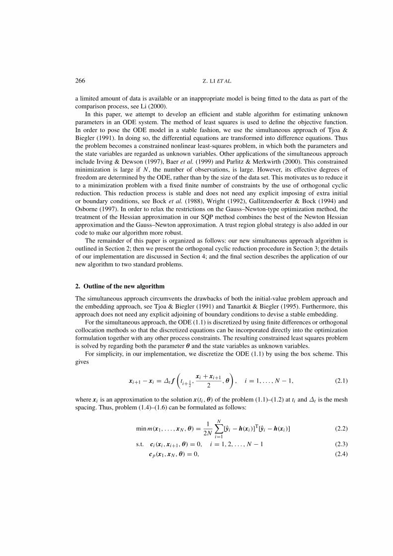
a limited amount of data is available or an inappropriate model is being fitted to the data as part of thecomparison process, see Li (2000).
In this paper, we attempt to develop an efficient and stable algorithm for estimating unknownparameters in an ODE system. The method of least squares is used to define the objective function.In order to pose the ODE model in a stable fashion, we use the simultaneous approach of Tjoa &Biegler (1991). In doing so, the differential equations are transformed into difference equations. Thusthe problem becomes a constrained nonlinear least-squares problem, in which both the parameters andthe state variables are regarded as unknown variables. Other applications of the simultaneous approachinclude Irving & Dewson (1997), Baer et al. (1999) and Parlitz & Merkwirth (2000). This constrainedminimization is large if N , the number of observations, is large. However, its effective degrees offreedom are determined by the ODE, rather than by the size of the data set. This motivates us to reduce itto a minimization problem with a fixed finite number of constraints by the use of orthogonal cyclicreduction. This reduction process is stable and does not need any explicit imposing of extra initialor boundary conditions, see Bock et al. (1988), Wright (1992), Gallitzendoerfer & Bock (1994) andOsborne (1997). In order to relax the restrictions on the Gauss–Newton-type optimization method, thetreatment of the Hessian approximation in our SQP method combines the best of the Newton Hessianapproximation and the Gauss–Newton approximation. A trust region global strategy is also added in ourcode to make our algorithm more robust.
The remainder of this paper is organized as follows: our new simultaneous approach algorithm isoutlined in Section 2; then we present the orthogonal cyclic reduction procedure in Section 3; the detailsof our implementation are discussed in Section 4; and the final section describes the application of ournew algorithm to two standard problems.
2. Outline of the new algorithm
The simultaneous approach circumvents the drawbacks of both the initial-value problem approach andthe embedding approach, see Tjoa & Biegler (1991) and Tanartkit & Biegler (1995). Furthermore, thisapproach does not need any explicit adjoining of boundary conditions to devise a stable embedding.
For the simultaneous approach, the ODE (1.1) is discretized by using finite differences or orthogonalcollocation methods so that the discretized equations can be incorporated directly into the optimizationformulation together with any other process constraints. The resulting constrained least squares problemis solved by regarding both the parameter θ and the state variables as unknown variables.
For simplicity, in our implementation, we discretize the ODE (1.1) by using the box scheme. Thisgives
xi+1 − xi = ∆t f(
ti+ 12,
xi + xi+1
2, θ
), i = 1, . . . , N − 1, (2.1)
where xi is an approximation to the solution x(ti , θ) of the problem (1.1)–(1.2) at ti and ∆t is the meshspacing. Thus, problem (1.4)–(1.6) can be formulated as follows:
min m(x1, . . . , xN , θ) = 1
2N
N∑i=1
[yi − h(xi )]T[yi − h(xi )] (2.2)
s.t. ci (xi , xi+1, θ) = 0, i = 1, 2, . . . , N − 1 (2.3)
cp(x1, xN , θ) = 0, (2.4)
PARAMETER ESTIMATION OF ODES 267
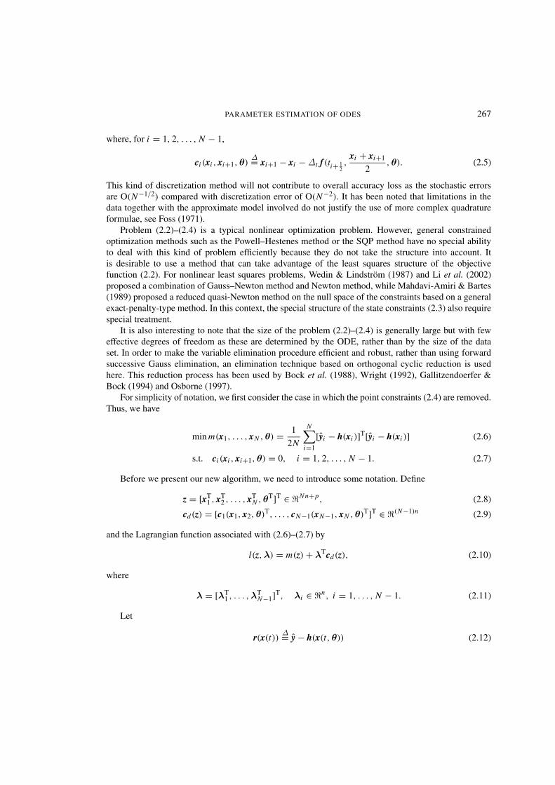
where, for i = 1, 2, . . . , N − 1,
ci (xi , xi+1, θ)∆= xi+1 − xi − ∆t f (ti+ 1
2,
xi + xi+1
2, θ). (2.5)
This kind of discretization method will not contribute to overall accuracy loss as the stochastic errorsare O(N−1/2) compared with discretization error of O(N−2). It has been noted that limitations in thedata together with the approximate model involved do not justify the use of more complex quadratureformulae, see Foss (1971).
Problem (2.2)–(2.4) is a typical nonlinear optimization problem. However, general constrainedoptimization methods such as the Powell–Hestenes method or the SQP method have no special abilityto deal with this kind of problem efficiently because they do not take the structure into account. Itis desirable to use a method that can take advantage of the least squares structure of the objectivefunction (2.2). For nonlinear least squares problems, Wedin & Lindstrom (1987) and Li et al. (2002)proposed a combination of Gauss–Newton method and Newton method, while Mahdavi-Amiri & Bartes(1989) proposed a reduced quasi-Newton method on the null space of the constraints based on a generalexact-penalty-type method. In this context, the special structure of the state constraints (2.3) also requirespecial treatment.
It is also interesting to note that the size of the problem (2.2)–(2.4) is generally large but with feweffective degrees of freedom as these are determined by the ODE, rather than by the size of the dataset. In order to make the variable elimination procedure efficient and robust, rather than using forwardsuccessive Gauss elimination, an elimination technique based on orthogonal cyclic reduction is usedhere. This reduction process has been used by Bock et al. (1988), Wright (1992), Gallitzendoerfer &Bock (1994) and Osborne (1997).
For simplicity of notation, we first consider the case in which the point constraints (2.4) are removed.Thus, we have
min m(x1, . . . , xN , θ) = 1
2N
N∑i=1
[yi − h(xi )]T[yi − h(xi )] (2.6)
s.t. ci (xi , xi+1, θ) = 0, i = 1, 2, . . . , N − 1. (2.7)
Before we present our new algorithm, we need to introduce some notation. Define
z = [xT1 , xT
2 , . . . , xTN , θT]T ∈ �Nn+p, (2.8)
cd(z) = [c1(x1, x2, θ)T, . . . , cN−1(xN−1, xN , θ)T]T ∈ �(N−1)n (2.9)
and the Lagrangian function associated with (2.6)–(2.7) by
l(z, λ) = m(z) + λTcd(z), (2.10)
where
λ = [λT1 , . . . ,λT
N−1]T, λi ∈ �n, i = 1, . . . , N − 1. (2.11)
Let
r(x(t))∆= y − h(x(t, θ)) (2.12)
268 Z. LI ET AL.
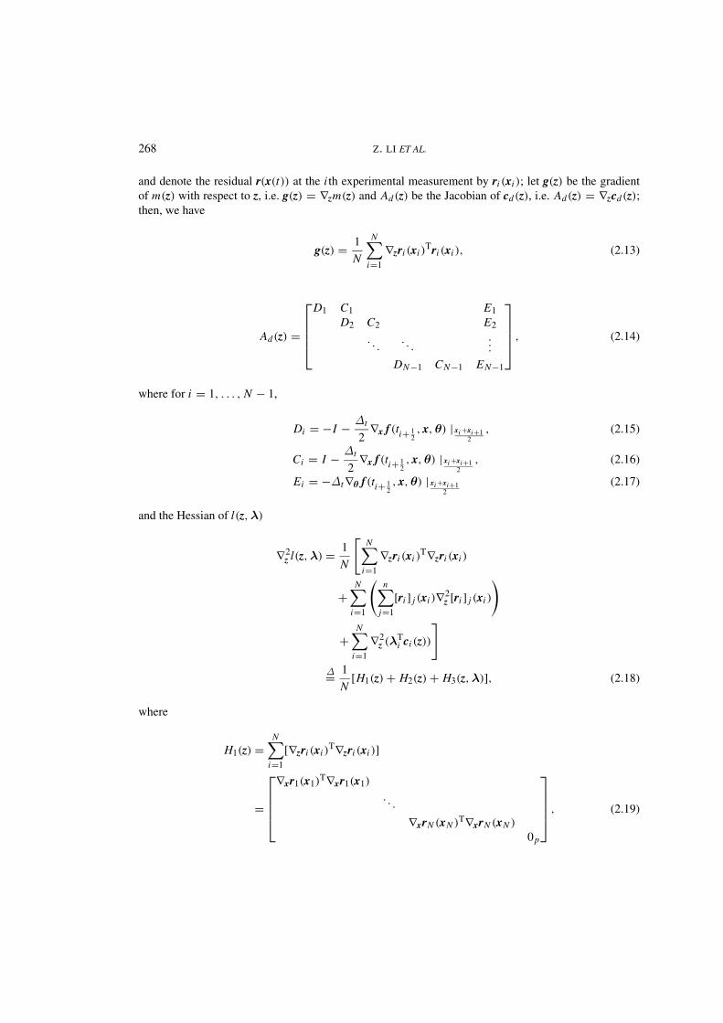
and denote the residual r(x(t)) at the i th experimental measurement by ri (xi ); let g(z) be the gradientof m(z) with respect to z, i.e. g(z) = ∇zm(z) and Ad(z) be the Jacobian of cd(z), i.e. Ad(z) = ∇zcd(z);then, we have
g(z) = 1
N
N∑i=1
∇zri (xi )Tri (xi ), (2.13)
Ad(z) =
D1 C1 E1D2 C2 E2
· · · · · · ···DN−1 CN−1 EN−1
, (2.14)
where for i = 1, . . . , N − 1,
Di = −I − ∆t
2∇x f (ti+ 1
2, x, θ) | xi +xi+1
2, (2.15)
Ci = I − ∆t
2∇x f (ti+ 1
2, x, θ) | xi +xi+1
2, (2.16)
Ei = −∆t∇θ f (ti+ 12, x, θ) | xi +xi+1
2(2.17)
and the Hessian of l(z, λ)
∇2z l(z, λ) = 1
N
[N∑
i=1
∇zri (xi )T∇zri (xi )
+N∑
i=1
(n∑
j=1
[ri ] j (xi )∇2z [ri ] j (xi )
)
+N∑
i=1
∇2z (λT
i ci (z))
]
∆= 1
N[H1(z) + H2(z) + H3(z, λ)], (2.18)
where
H1(z) =N∑
i=1
[∇zri (xi )T∇zri (xi )]
=
∇xr1(x1)T∇xr1(x1)
· · ·∇xrN (xN )T∇xrN (xN )
0p
, (2.19)
PARAMETER ESTIMATION OF ODES 269
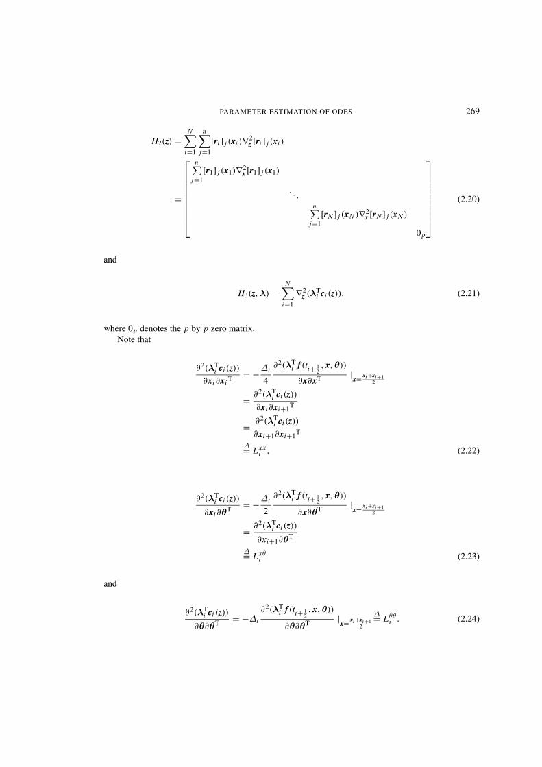
H2(z) =N∑
i=1
n∑j=1
[ri ] j (xi )∇2z [ri ] j (xi )
=
n∑j=1
[r1] j (x1)∇2x [r1] j (x1)
· · ·n∑
j=1[rN ] j (xN )∇2
x [rN ] j (xN )
0p
(2.20)
and
H3(z, λ) =N∑
i=1
∇2z (λT
i ci (z)), (2.21)
where 0p denotes the p by p zero matrix.Note that
∂2(λTi ci (z))
∂xi∂xiT = −∆t
4
∂2(λTi f (ti+ 1
2, x, θ))
∂x∂xT |x= xi +xi+1
2
= ∂2(λTi ci (z))
∂xi∂xi+1T
= ∂2(λTi ci (z))
∂xi+1∂xi+1T
∆= Lxxi , (2.22)
∂2(λTi ci (z))
∂xi∂θT = −∆t
2
∂2(λTi f (ti+ 1
2, x, θ))
∂x∂θT |x= xi +xi+1
2
= ∂2(λTi ci (z))
∂xi+1∂θT
∆= Lxθi (2.23)
and
∂2(λTi ci (z))
∂θ∂θT = −∆t
∂2(λTi f (ti+ 1
2, x, θ))
∂θ∂θT |x= xi +xi+1
2
∆= Lθθi . (2.24)
270 Z. LI ET AL.
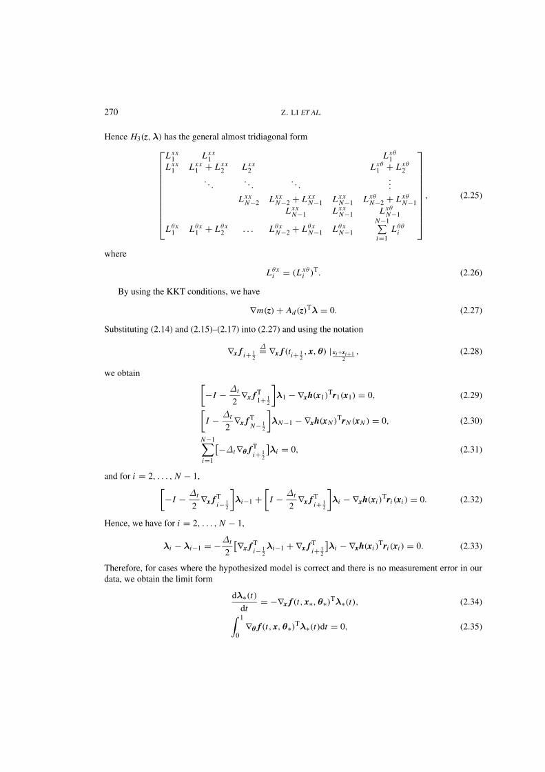
Hence H3(z, λ) has the general almost tridiagonal form
Lxx1 Lxx
1 Lxθ1
Lxx1 Lxx
1 + Lxx2 Lxx
2 Lxθ1 + Lxθ
2
· · · · · · · · · ···Lxx
N−2 LxxN−2 + Lxx
N−1 LxxN−1 Lxθ
N−2 + LxθN−1
LxxN−1 Lxx
N−1 LxθN−1
Lθx1 Lθx
1 + Lθx2 . . . Lθx
N−2 + LθxN−1 Lθx
N−1
N−1∑i=1
Lθθi
, (2.25)
where
Lθxi = (Lxθ
i )T. (2.26)
By using the KKT conditions, we have
∇m(z) + Ad(z)Tλ = 0. (2.27)
Substituting (2.14) and (2.15)–(2.17) into (2.27) and using the notation
∇x f i+ 12
∆= ∇x f (ti+ 12, x, θ) | xi +xi+1
2, (2.28)
we obtain [−I − ∆t
2∇x f T
1+ 12
]λ1 − ∇xh(x1)
Tr1(x1) = 0, (2.29)[I − ∆t
2∇x f T
N− 12
]λN−1 − ∇xh(xN )TrN (xN ) = 0, (2.30)
N−1∑i=1
[−∆t∇θ f Ti+ 1
2
]λi = 0, (2.31)
and for i = 2, . . . , N − 1,[−I − ∆t
2∇x f T
i− 12
]λi−1 +
[I − ∆t
2∇x f T
i+ 12
]λi − ∇xh(xi )
Tri (xi ) = 0. (2.32)
Hence, we have for i = 2, . . . , N − 1,
λi − λi−1 = −∆t
2
[∇x f Ti− 1
2λi−1 + ∇x f T
i+ 12
]λi − ∇xh(xi )
Tri (xi ) = 0. (2.33)
Therefore, for cases where the hypothesized model is correct and there is no measurement error in ourdata, we obtain the limit form
dλ∗(t)dt
= −∇x f (t, x∗, θ∗)Tλ∗(t), (2.34)∫ 1
0∇θ f (t, x, θ∗)Tλ∗(t)dt = 0, (2.35)
PARAMETER ESTIMATION OF ODES 271
where x∗(t) is determined by
dx∗dt
= f (t, x∗, θ∗). (2.36)
It is interesting to note that the trivial solution of problem (2.34)–(2.35) is
λ∗(t) = 0. (2.37)
Our numerical results confirm this theory: we observed that, as an approximation to λ∗(t) in the casewhere the number of observations N is large, λN (t) is small. Therefore, for simplicity of testing, initiallywe choose λi = 0 for i = 1, . . . , N − 1.
In cases where measurement errors are present ri (x∗(ti )) = εi = ∫ titi−1
dw, where w is a Wienerprocess, we will have a stochastic differential equation for λ∗(t).
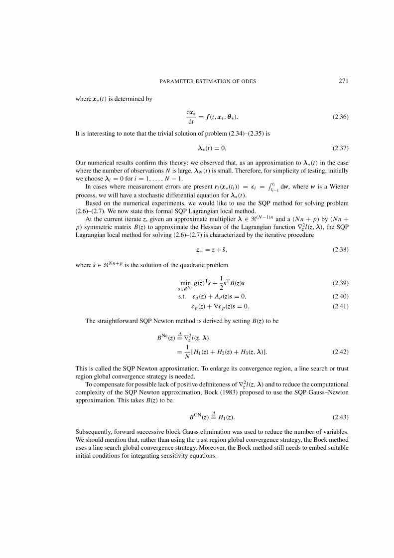
Based on the numerical experiments, we would like to use the SQP method for solving problem(2.6)–(2.7). We now state this formal SQP Lagrangian local method.
At the current iterate z, given an approximate multiplier λ ∈ �(N−1)n and a (Nn + p) by (Nn +p) symmetric matrix B(z) to approximate the Hessian of the Lagrangian function ∇2
z l(z, λ), the SQPLagrangian local method for solving (2.6)–(2.7) is characterized by the iterative procedure
z+ = z + s, (2.38)
where s ∈ �Nn+p is the solution of the quadratic problem
mins∈RNn
g(z)Ts + 1
2sT B(z)s (2.39)
s.t. cd(z) + Ad(z)s = 0, (2.40)
cp(z) + ∇cp(z)s = 0. (2.41)
The straightforward SQP Newton method is derived by setting B(z) to be
BNe(z)∆= ∇2
z l(z, λ)
= 1
N[H1(z) + H2(z) + H3(z, λ)]. (2.42)
This is called the SQP Newton approximation. To enlarge its convergence region, a line search or trustregion global convergence strategy is needed.
To compensate for possible lack of positive definiteness of ∇2z l(z, λ) and to reduce the computational
complexity of the SQP Newton approximation, Bock (1983) proposed to use the SQP Gauss–Newtonapproximation. This takes B(z) to be
BGN(z)∆= H1(z). (2.43)
Subsequently, forward successive block Gauss elimination was used to reduce the number of variables.We should mention that, rather than using the trust region global convergence strategy, the Bock methoduses a line search global convergence strategy. Moreover, the Bock method still needs to embed suitableinitial conditions for integrating sensitivity equations.
272 Z. LI ET AL.
The use of the SQP Gauss–Newton approximation is recommended only if the hypothesized modelis correct and the sample data set is large enough. If these assumptions hold, it has the advantages ofefficiency and stability. Otherwise, this kind of approximation could result in poor performance. In orderto improve the performance of the SQP Gauss–Newton approximation, Biegler and his co-workers (Tjoa& Biegler, 1991 and Tanartkit & Biegler, 1995) proposed a simple hybrid SQP method based on a teston the relative merit function value. If the relative merit function value is small, the SQP Gauss–Newtonapproximation is used; otherwise, the choice is the SQP BFGS approximation. However, this switchingrule may refuse the use of the SQP Gauss–Newton approximation even if its performance is satisfactory.Thus, it reduces the efficiency of the algorithm. If the data set is large, then the law of large numberscan be used to show that the size of the residuals is not the point. If the sample size is large enough, theeffect of these large residuals can be pinned down due to cancellation.
The size of problem (2.39)–(2.40) is large but it has few effective degrees of freedom, so thevariable reduction method has a natural application, see Fletcher (1987, pp. 230–236). To take advantageof the almost block-bidiagonal structure of the linearized constraints arising from the ODE, forwardsuccessive block Gauss elimination was used in Bock (1983). This reduction technique is similar to thecompactification numerical method for the boundary value problems of ODEs for it can suffer frominstability, much like the single shooting method, see Ascher et al. (1995). In the earlier version of theTjoa and Biegler method in Tjoa & Biegler (1991) and Tanartkit & Biegler (1995), a complete pivotingGauss elimination method was used without taking advantage of the almost block-bidiagonal structure.Later, Biegler (1998) proposed the use of the block Gauss elimination method to take advantage of thealmost block-bidiagonal structure. However, in these examples, the aim of the elimination is to simplifyoverhead calculation rather than to explicitly reduce the number of variables in the optimization problem.
For these reasons, a new SQP algorithm is proposed that incorporates a number of novel features:
1. A different approach to distinguish between two competing models (the SQP Gauss–Newtonapproximation and the SQP Newton approximation) is taken: our local quadratic model containsthe use of either the SQP Gauss–Newton approximation or the SQP Newton approximation. Thechoice is determined by numerical performance, not by the size of residuals. Our algorithmpermits the use of the SQP Gauss–Newton approximation even for large merit function valueproblems if its performance is better. This will allow us to choose the SQP Gauss–Newtonapproximation as often as possible;
2. The orthogonal cyclic reduction process is used for variable reduction. This procedure avoidsthe hard task of explicitly adjoining extra initial or boundary conditions to take up the intrinsicdegrees of freedom in the solution set of the differential equations in order to guarantee that theestimation problem is stably posed;
3. The trust region global convergence strategy is used. This makes our algorithm more robust.
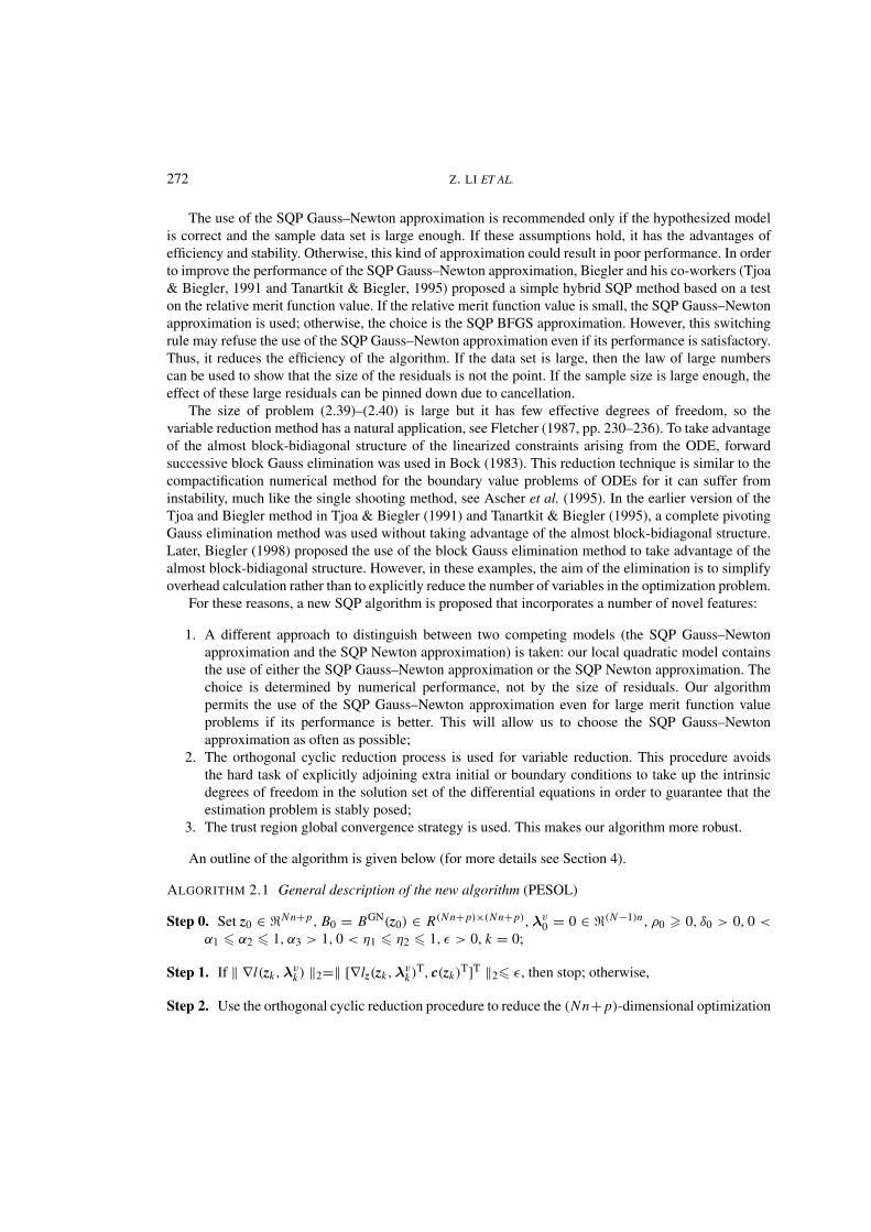
An outline of the algorithm is given below (for more details see Section 4).
ALGORITHM 2.1 General description of the new algorithm (PESOL)
Step 0. Set z0 ∈ �Nn+p, B0 = BGN(z0) ∈ R(Nn+p)×(Nn+p), λv0 = 0 ∈ �(N−1)n, ρ0 � 0, δ0 > 0, 0 <
α1 � α2 � 1, α3 > 1, 0 < η1 � η2 � 1, ε > 0, k = 0;
Step 1. If ‖ ∇l(zk, λvk ) ‖2=‖ [∇lz(zk, λ
vk )
T, c(zk)T]T ‖2� ε, then stop; otherwise,
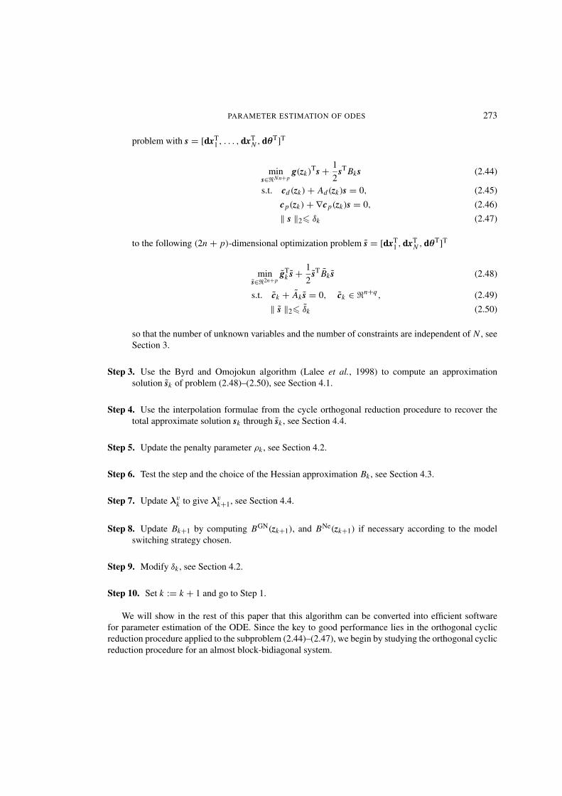
Step 2. Use the orthogonal cyclic reduction procedure to reduce the (Nn+ p)-dimensional optimization
PARAMETER ESTIMATION OF ODES 273
problem with s = [dxT1 , . . . , dxT
N , dθT]T
mins∈�Nn+p
g(zk)Ts + 1
2sT Bks (2.44)
s.t. cd(zk) + Ad(zk)s = 0, (2.45)
cp(zk) + ∇cp(zk)s = 0, (2.46)
‖ s ‖2� δk (2.47)
to the following (2n + p)-dimensional optimization problem s = [dxT1 , dxT
N , dθT]T
mins∈�2n+p
gTk s + 1
2sT Bk s (2.48)
s.t. ck + Ak s = 0, ck ∈ �n+q , (2.49)
‖ s ‖2� δk (2.50)
so that the number of unknown variables and the number of constraints are independent of N , seeSection 3.
Step 3. Use the Byrd and Omojokun algorithm (Lalee et al., 1998) to compute an approximationsolution sk of problem (2.48)–(2.50), see Section 4.1.
Step 4. Use the interpolation formulae from the cycle orthogonal reduction procedure to recover thetotal approximate solution sk through sk , see Section 4.4.
Step 5. Update the penalty parameter ρk , see Section 4.2.
Step 6. Test the step and the choice of the Hessian approximation Bk , see Section 4.3.
Step 7. Update λvk to give λv
k+1, see Section 4.4.
Step 8. Update Bk+1 by computing BGN(zk+1), and BNe(zk+1) if necessary according to the modelswitching strategy chosen.
Step 9. Modify δk , see Section 4.2.
Step 10. Set k := k + 1 and go to Step 1.
We will show in the rest of this paper that this algorithm can be converted into efficient softwarefor parameter estimation of the ODE. Since the key to good performance lies in the orthogonal cyclicreduction procedure applied to the subproblem (2.44)–(2.47), we begin by studying the orthogonal cyclicreduction procedure for an almost block-bidiagonal system.
274 Z. LI ET AL.
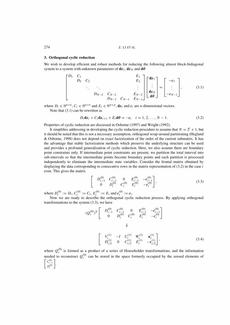
3. Orthogonal cyclic reduction
We wish to develop efficient and robust methods for reducing the following almost block-bidiagonalsystem to a system with unknown parameters of dx1, dxN and dθ
D1 C1 E1D2 C2 E2
· · · · · · ···DN−2 CN−2 EN−2
DN−1 CN−1 EN−1
dx1
···dxN
dθ
=
−c1
···−cN−1
, (3.1)
where Di ∈ �n×n , Ci ∈ �n×n and Ei ∈ �n×p, dxi and ci are n-dimensional vectors.Note that (3.1) can be rewritten as
Di dxi + Ci dxi+1 + Ei dθ = −ci i = 1, 2, . . . , N − 1. (3.2)
Properties of cyclic reduction are discussed in Osborne (1997) and Wright (1992).It simplifies addressing in developing the cyclic reduction procedure to assume that N = 2l + 1, but
it should be noted that this is not a necessary assumption, orthogonal wrap-around partitioning (Hegland& Osborne, 1998) does not depend on exact factorization of the order of the current submatrix. It hasthe advantage that stable factorization methods which preserve the underlying structure can be usedand provides a profound generalization of cyclic reduction. Here, we also assume there are boundarypoint constraints only. If intermediate point constraints are present, we partition the total interval intosub-intervals so that the intermediate points become boundary points and each partition is processedindependently to eliminate the intermediate state variables. Consider the frontal matrix obtained bydisplaying the data corresponding to consecutive rows in the matrix representation of (3.2) in the case ieven. This gives the matrix [
D(0)i−1 C (0)
i−1 0 E (0)i−1 −c(0)
i−1
0 D(0)i C (0)
i E (0)i −c(0)
i
], (3.3)
where D(0)i := Di , C (0)
i := Ci , E (0)i := Ei and c(0)
i := ci .Now we are ready to describe the orthogonal cyclic reduction process. By applying orthogonal
transformations to the system (3.3), we have
(Q(0)i )T
[D(0)
i−1 C (0)i−1 0 E (0)
i−1 −c(0)i−1
0 D(0)i C (0)
i E (0)i −c(0)
i
]
⇓[
V (1)i −I U (1)
i W (1)i u(1)
i
D(1)i/2 0 C (1)
i/2 E (1)i −c(1)
i/2
], (3.4)
where Q(0)i is formed as a product of a series of Householder transformations, and the information
needed to reconstruct Q(0)i can be stored in the space formerly occupied by the zeroed elements of[
C(0)i−1
D(0)i
].
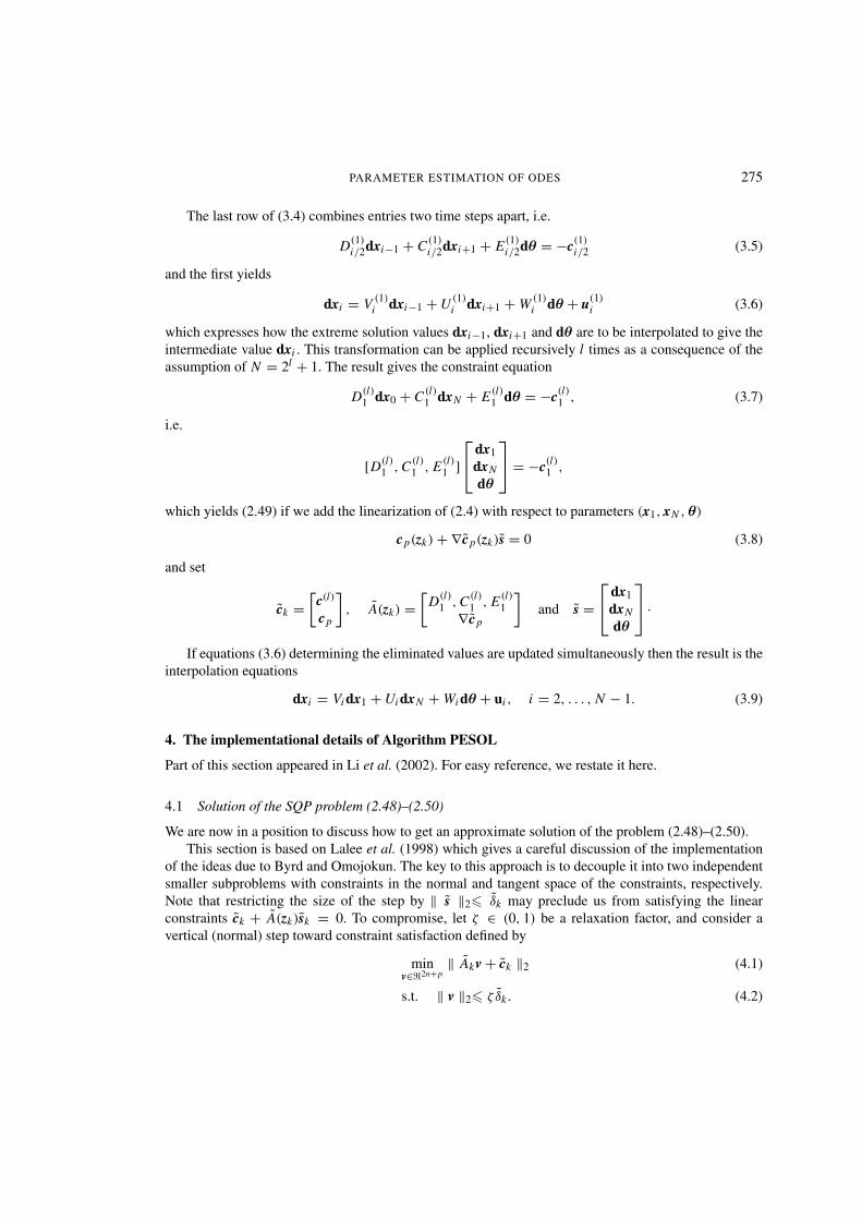
PARAMETER ESTIMATION OF ODES 275
The last row of (3.4) combines entries two time steps apart, i.e.
D(1)i/2dxi−1 + C (1)
i/2dxi+1 + E (1)i/2dθ = −c(1)
i/2 (3.5)
and the first yields
dxi = V (1)i dxi−1 + U (1)
i dxi+1 + W (1)i dθ + u(1)
i (3.6)
which expresses how the extreme solution values dxi−1, dxi+1 and dθ are to be interpolated to give theintermediate value dxi . This transformation can be applied recursively l times as a consequence of theassumption of N = 2l + 1. The result gives the constraint equation
D(l)1 dx0 + C (l)
1 dxN + E (l)1 dθ = −c(l)
1 , (3.7)
i.e.
[D(l)1 , C (l)
1 , E (l)1 ]
dx1
dxN
dθ
= −c(l)
1 ,
which yields (2.49) if we add the linearization of (2.4) with respect to parameters (x1, xN , θ)
cp(zk) + ∇ cp(zk)s = 0 (3.8)
and set
ck =[
c(l)
cp
], A(zk) =
[D(l)
1 , C (l)1 , E (l)
1∇ cp
]and s =
dx1
dxN
dθ
·
If equations (3.6) determining the eliminated values are updated simultaneously then the result is theinterpolation equations
dxi = Vi dx1 + Ui dxN + Wi dθ + ui , i = 2, . . . , N − 1. (3.9)
4. The implementational details of Algorithm PESOL
Part of this section appeared in Li et al. (2002). For easy reference, we restate it here.
4.1 Solution of the SQP problem (2.48)–(2.50)
We are now in a position to discuss how to get an approximate solution of the problem (2.48)–(2.50).This section is based on Lalee et al. (1998) which gives a careful discussion of the implementation
of the ideas due to Byrd and Omojokun. The key to this approach is to decouple it into two independentsmaller subproblems with constraints in the normal and tangent space of the constraints, respectively.Note that restricting the size of the step by ‖ s ‖2� δk may preclude us from satisfying the linearconstraints ck + A(zk)sk = 0. To compromise, let ζ ∈ (0, 1) be a relaxation factor, and consider avertical (normal) step toward constraint satisfaction defined by
minv∈�2n+p
‖ Akv + ck ‖2 (4.1)
s.t. ‖ v ‖2� ζ δk . (4.2)
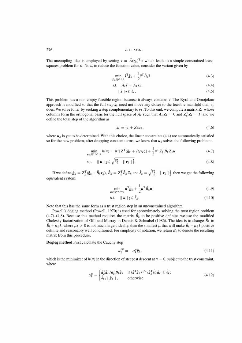
276 Z. LI ET AL.
The uncoupling idea is employed by setting v = A(zk)Tw which leads to a simple constrained least-
squares problem for w. Now, to reduce the function value, consider the variant given by
mins∈�2n+p
sTgk + 1
2sT Bk s (4.3)
s.t. Ak s = Akvk, (4.4)
‖ s ‖2� δk . (4.5)
This problem has a non-empty feasible region because it always contains v. The Byrd and Omojokunapproach is modified so that the full step sk need not move any closer to the feasible manifold than vk
does. We solve for sk by seeking a step complementary to vk . To this end, we compute a matrix Zk whosecolumns form the orthogonal basis for the null space of Ak such that Ak Zk = 0 and ZT
k Zk = I , and wedefine the total step of the algorithm as
sk = vk + Zkuk, (4.6)
where uk is yet to be determined. With this choice, the linear constraints (4.4) are automatically satisfiedso for the new problem, after dropping constant terms, we know that uk solves the following problem:
minu∈�n+p−q
h(u) = uT[ZT(gk + Bkvk)] + 1
2uT ZT
k Bk Zku (4.7)
s.t. ‖ u ‖2�√
δ2k − ‖ vk ‖2
2. (4.8)
If we define gk = ZTk (gk + Bkvk), Bk = ZT
k Bk Zk and δk =√
δ2k − ‖ vk ‖2
2, then we get the followingequivalent system:
minu∈�n+p−q
uTgk + 1
2uT Bku (4.9)
s.t. ‖ u ‖2� δk . (4.10)
Note that this has the same form as a trust region step in an unconstrained algorithm.Powell’s dogleg method (Powell, 1970) is used for approximately solving the trust region problem
(4.7)–(4.8). Because this method requires the matrix Bk to be positive definite, we use the modifiedCholesky factorization of Gill and Murray in Dennis & Schnabel (1986). The idea is to change Bk toBk +µk I , where µk > 0 is not much larger, ideally, than the smallest µ that will make Bk +µk I positivedefinite and reasonably well conditioned. For simplicity of notation, we retain Bk to denote the resultingmatrix from this procedure.
Dogleg method First calculate the Cauchy step
ucpk = −αu
k gk, (4.11)
which is the minimizer of h(u) in the direction of steepest descent at u = 0, subject to the trust constraint,where
αuk =
{gT
k gk/gTk Bk gk if (gTgk)
3/2/gTk Bk gk � δk;
δk/‖ gk ‖2 otherwise(4.12)
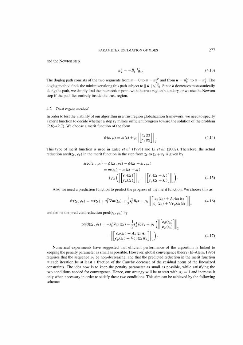
PARAMETER ESTIMATION OF ODES 277
and the Newton step
unk = −B−1
k gk . (4.13)
The dogleg path consists of the two segments from u = 0 to u = ucpk and from u = ucp
k to u = unk . The
dogleg method finds the minimizer along this path subject to ‖ u ‖� δk . Since h decreases monotonicallyalong the path, we simply find the intersection point with the trust region boundary, or we use the Newtonstep if the path lies entirely inside the trust region.
4.2 Trust region method
In order to test the viability of our algorithm in a trust region globalization framework, we need to specifya merit function to decide whether a step sk makes sufficient progress toward the solution of the problem(2.6)–(2.7). We choose a merit function of the form
φ(z, ρ) = m(z) + ρ
∥∥∥∥[
cd(z)cp(z)
]∥∥∥∥2. (4.14)
This type of merit function is used in Lalee et al. (1998) and Li et al. (2002). Therefore, the actualreduction ared(zk, ρk) in the merit function in the step from zk to zk + sk is given by
ared(zk, ρk) = φ(zk, ρk) − φ(zk + sk, ρk)
= m(zk) − m(zk + sk)
+ρk
(∥∥∥∥[
cd(zk)
cp(zk)
]∥∥∥∥2−
∥∥∥∥[
cd(zk + sk)
cp(zk + sk)
]∥∥∥∥2
). (4.15)
Also we need a prediction function to predict the progress of the merit function. We choose this as
ψ(zk, ρk) = m(zk) + sTk ∇m(zk) + 1
2sT
k Bks + ρk
∥∥∥∥[
cd(zk) + Ad(zk)sk
cp(zk) + ∇cp(zk)sk
]∥∥∥∥2
(4.16)
and define the predicted reduction pred(zk, ρk) by
pred(zk, ρk) = −sTk ∇m(zk) − 1
2sT
k Bksk + ρk
(∥∥∥∥[
cd(zk)
cp(zk)
]∥∥∥∥2
−∥∥∥∥[
cd(zk) + Ad(zk)sk
cp(zk) + ∇cp(zk)sk
]∥∥∥∥2
). (4.17)
Numerical experiments have suggested that efficient performance of the algorithm is linked tokeeping the penalty parameter as small as possible. However, global convergence theory (El-Alem, 1995)requires that the sequence ρk be non-decreasing, and that the predicted reduction in the merit functionat each iteration be at least a fraction of the Cauchy decrease of the residual norm of the linearizedconstraints. The idea now is to keep the penalty parameter as small as possible, while satisfying thetwo conditions needed for convergence. Hence, our strategy will be to start with ρ0 = 1 and increase itonly when necessary in order to satisfy these two conditions. This aim can be achieved by the followingscheme:

278 Z. LI ET AL.
(a) If pred(zk, ρk) � ξρk
(∥∥∥[cd (zk )cp(zk )
]∥∥∥2−
∥∥∥[cd (zk )+Ad (zk )sk
cp(zk )+∇cp(zk )sk
]∥∥∥2
),
where ξ ∈ (0, 1), then we set
ρk+1 := ρk; (4.18)
(b) else, we set
ρk+1 := 1
1 − ξ· sT
k ∇m(zk) + 12 sT
k Bksk∥∥∥∥[
cd(zk)
cp(zk)
]∥∥∥∥2−
∥∥∥∥[
cd(zk) + Ad(zk)sk
cp(zk) + ∇cp(zk)sk
]∥∥∥∥2
+ 0·0001, (4.19)
where adding 0·0001 is to make sure that ρk+1 is not too small; choice of other small values doesnot appear critical, the value of 0·0001 is typically used.
Once zk+1 has been found, we decide which trust region radius to use first when seeking zk+2. The radiuschosen is as follows:
(a) if
ared(zpk+1, ρk+1)
pred(zpk+1, ρk+1)
� 0·75, (4.20)
we set δk+1 = min(2δk, δ∗), where δ∗ is the maximum step length allowed in the algorithm;(b) else if
ared(zpk+1, ρk+1)
pred(zpk+1, ρk+1)
< 0·1, (4.21)
we set δk+1 to be a fraction of the failed step length such that
δk+1 ∈ [0·1 ‖ sk ‖2, 0·5 ‖ sk ‖2]. (4.22)
The precise value is computed by assuming that the ratio of actual to predicted reduction is alinear function w(‖ s ‖2) of the step length ‖ s ‖2, satisfying w(0) = 1 and w(‖ sk ‖2) =ared(zk+1, ρk+1)/ pred(zk+1, ρk+1), and then finding the value of ‖ s ‖2 where w(‖ s ‖) equalsη1 by the following formula:
δk+1 = 1 − η1
1 − (ared(zk+1, ρk+1)/ pred(zk+1, ρk+1))‖ sk ‖2; (4.23)
this value is truncated such that δk+1 ∈ [0·1 ‖ sk ‖2, 0·5 ‖ sk ‖2];(c) else, we keep the same radius, i.e. set
δk+1 = min(2δk, δ∗). (4.24)
4.3 Model switching strategy
Our experiments show that for some steps the SQP Gauss–Newton approximation works better than theSQP Newton approximation, so it seems useful to have some way to decide which approximation to use
PARAMETER ESTIMATION OF ODES 279
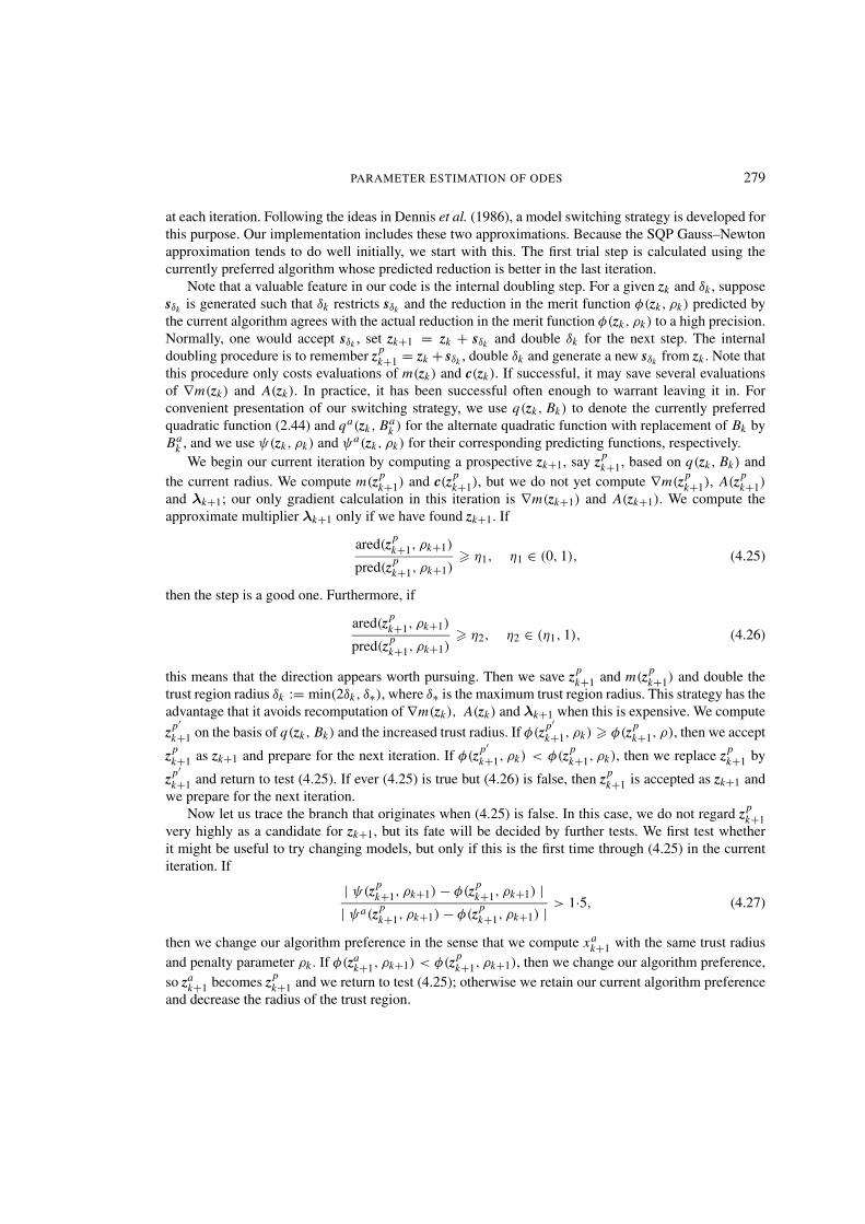
at each iteration. Following the ideas in Dennis et al. (1986), a model switching strategy is developed forthis purpose. Our implementation includes these two approximations. Because the SQP Gauss–Newtonapproximation tends to do well initially, we start with this. The first trial step is calculated using thecurrently preferred algorithm whose predicted reduction is better in the last iteration.
Note that a valuable feature in our code is the internal doubling step. For a given zk and δk , supposesδk is generated such that δk restricts sδk and the reduction in the merit function φ(zk, ρk) predicted bythe current algorithm agrees with the actual reduction in the merit function φ(zk, ρk) to a high precision.Normally, one would accept sδk , set zk+1 = zk + sδk and double δk for the next step. The internaldoubling procedure is to remember zp
k+1 = zk + sδk , double δk and generate a new sδk from zk . Note thatthis procedure only costs evaluations of m(zk) and c(zk). If successful, it may save several evaluationsof ∇m(zk) and A(zk). In practice, it has been successful often enough to warrant leaving it in. Forconvenient presentation of our switching strategy, we use q(zk, Bk) to denote the currently preferredquadratic function (2.44) and qa(zk, Ba
k ) for the alternate quadratic function with replacement of Bk byBa
k , and we use ψ(zk, ρk) and ψa(zk, ρk) for their corresponding predicting functions, respectively.We begin our current iteration by computing a prospective zk+1, say zp
k+1, based on q(zk, Bk) andthe current radius. We compute m(zp
k+1) and c(zpk+1), but we do not yet compute ∇m(zp
k+1), A(zpk+1)
and λk+1; our only gradient calculation in this iteration is ∇m(zk+1) and A(zk+1). We compute theapproximate multiplier λk+1 only if we have found zk+1. If
ared(zpk+1, ρk+1)
pred(zpk+1, ρk+1)
� η1, η1 ∈ (0, 1), (4.25)
then the step is a good one. Furthermore, if
ared(zpk+1, ρk+1)
pred(zpk+1, ρk+1)
� η2, η2 ∈ (η1, 1), (4.26)
this means that the direction appears worth pursuing. Then we save zpk+1 and m(zp
k+1) and double thetrust region radius δk := min(2δk, δ∗), where δ∗ is the maximum trust region radius. This strategy has theadvantage that it avoids recomputation of ∇m(zk), A(zk) and λk+1 when this is expensive. We compute
zp′k+1 on the basis of q(zk, Bk) and the increased trust radius. If φ(zp′
k+1, ρk) � φ(zpk+1, ρ), then we accept
zpk+1 as zk+1 and prepare for the next iteration. If φ(zp′
k+1, ρk) < φ(zpk+1, ρk), then we replace zp
k+1 by
zp′k+1 and return to test (4.25). If ever (4.25) is true but (4.26) is false, then zp
k+1 is accepted as zk+1 andwe prepare for the next iteration.
Now let us trace the branch that originates when (4.25) is false. In this case, we do not regard zpk+1
very highly as a candidate for zk+1, but its fate will be decided by further tests. We first test whetherit might be useful to try changing models, but only if this is the first time through (4.25) in the currentiteration. If
| ψ(zpk+1, ρk+1) − φ(zp
k+1, ρk+1) || ψa(zp
k+1, ρk+1) − φ(zpk+1, ρk+1) | > 1·5, (4.27)
then we change our algorithm preference in the sense that we compute xak+1 with the same trust radius
and penalty parameter ρk . If φ(zak+1, ρk+1) < φ(zp
k+1, ρk+1), then we change our algorithm preference,so za
k+1 becomes zpk+1 and we return to test (4.25); otherwise we retain our current algorithm preference
and decrease the radius of the trust region.
280 Z. LI ET AL.
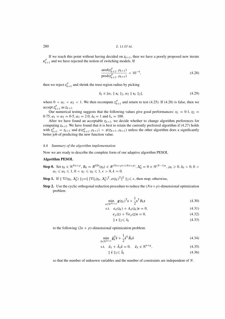
If we reach this point without having decided on zk+1, then we have a poorly proposed new iteratexp
k+1 and we have rejected the notion of switching models. If
ared(zpk+1, ρk+1)
pred(zpk+1, ρk+1)
< 10−4, (4.28)
then we reject zpk+1 and shrink the trust region radius by picking
δk ∈ [α1 ‖ sk ‖2, α2 ‖ sk ‖2], (4.29)
where 0 < α1 < α2 < 1. We then recompute zpk+1 and return to test (4.25). If (4.28) is false, then we
accept zpk+1 as zk+1.
Our numerical testing suggests that the following values give good performances: η1 = 0·1, η2 =0·75, α1 = α2 = 0·5, α3 = 2·0, δ0 = 1 and δ∗ = 100.
After we have found an acceptable zk+1, we decide whether to change algorithm preferences forcomputing zk+2. We have found that it is best to retain the currently preferred algorithm if (4.27) holdswith zp
k+1 = zk+1 and φ(zak+1, ρk+1) > φ(zk+1, ρk+1) unless the other algorithm does a significantly
better job of predicting the new function value.
4.4 Summary of the algorithm implementation
Now we are ready to describe the complete form of our adaptive algorithm PESOL
Algorithm PESOL
Step 0. Set z0 ∈ �Nn+p, B0 = BGN(z0) ∈ R(Nn+p)×(Nn+p), λv0 = 0 ∈ �(N−1)n, ρ0 � 0, δ0 > 0, 0 <
α1 � α2 � 1, 0 < η1 � η2 � 1, ε > 0, k = 0.
Step 1. If ‖ ∇l(zk, λvk ) ‖2=‖ [∇lz(zk, λ
vk )
T, c(zk)T]T ‖2� ε, then stop; otherwise,
Step 2. Use the cyclic orthogonal reduction procedure to reduce the (Nn+ p)-dimensional optimizationproblem
mins∈�Nn+p
g(zk)Ts + 1
2sT Bks (4.30)
s.t. cd(zk) + Ad(zk)s = 0, (4.31)
cp(z) + ∇cp(z)s = 0, (4.32)
‖ s ‖2� δk (4.33)
to the following (2n + p)-dimensional optimization problem:
mins∈�2n+p
gTk s + 1
2sT Bk s (4.34)
s.t. ck + Ak s = 0, ck ∈ �n+q , (4.35)
‖ s ‖2� δk (4.36)
so that the number of unknown variables and the number of constraints are independent of N .
PARAMETER ESTIMATION OF ODES 281
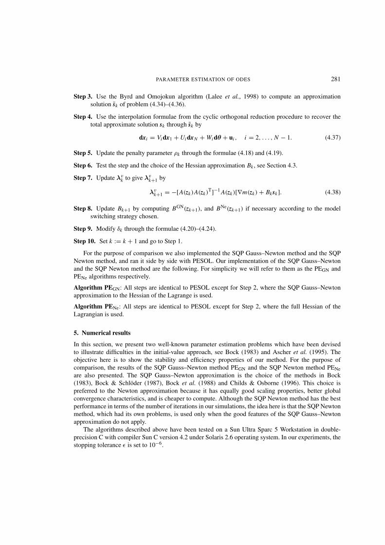
Step 3. Use the Byrd and Omojokun algorithm (Lalee et al., 1998) to compute an approximationsolution sk of problem (4.34)–(4.36).
Step 4. Use the interpolation formulae from the cyclic orthogonal reduction procedure to recover thetotal approximate solution sk through sk by
dxi = Vi dx1 + Ui dxN + Wi dθ + ui , i = 2, . . . , N − 1. (4.37)
Step 5. Update the penalty parameter ρk through the formulae (4.18) and (4.19).
Step 6. Test the step and the choice of the Hessian approximation Bk , see Section 4.3.
Step 7. Update λvk to give λv
k+1 by
λvk+1 = −[A(zk)A(zk)
T]−1 A(zk)[∇m(zk) + Bksk]. (4.38)
Step 8. Update Bk+1 by computing BGN(zk+1), and BNe(zk+1) if necessary according to the modelswitching strategy chosen.
Step 9. Modify δk through the formulae (4.20)–(4.24).
Step 10. Set k := k + 1 and go to Step 1.
For the purpose of comparison we also implemented the SQP Gauss–Newton method and the SQPNewton method, and ran it side by side with PESOL. Our implementation of the SQP Gauss–Newtonand the SQP Newton method are the following. For simplicity we will refer to them as the PEGN andPENe algorithms respectively.
Algorithm PEGN: All steps are identical to PESOL except for Step 2, where the SQP Gauss–Newtonapproximation to the Hessian of the Lagrange is used.
Algorithm PENe: All steps are identical to PESOL except for Step 2, where the full Hessian of theLagrangian is used.
5. Numerical results
In this section, we present two well-known parameter estimation problems which have been devisedto illustrate difficulties in the initial-value approach, see Bock (1983) and Ascher et al. (1995). Theobjective here is to show the stability and efficiency properties of our method. For the purpose ofcomparison, the results of the SQP Gauss–Newton method PEGN and the SQP Newton method PENeare also presented. The SQP Gauss–Newton approximation is the choice of the methods in Bock(1983), Bock & Schloder (1987), Bock et al. (1988) and Childs & Osborne (1996). This choice ispreferred to the Newton approximation because it has equally good scaling properties, better globalconvergence characteristics, and is cheaper to compute. Although the SQP Newton method has the bestperformance in terms of the number of iterations in our simulations, the idea here is that the SQP Newtonmethod, which had its own problems, is used only when the good features of the SQP Gauss–Newtonapproximation do not apply.
The algorithms described above have been tested on a Sun Ultra Sparc 5 Workstation in double-precision C with compiler Sun C version 4.2 under Solaris 2.6 operating system. In our experiments, thestopping tolerance ε is set to 10−6.
282 Z. LI ET AL.
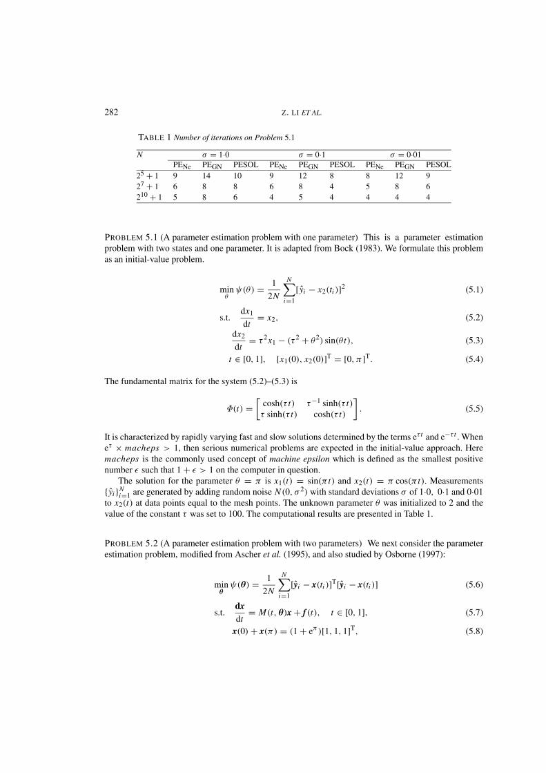
TABLE 1 Number of iterations on Problem 5.1
N σ = 1·0 σ = 0·1 σ = 0·01PENe PEGN PESOL PENe PEGN PESOL PENe PEGN PESOL
25 + 1 9 14 10 9 12 8 8 12 927 + 1 6 8 8 6 8 4 5 8 6210 + 1 5 8 6 4 5 4 4 4 4
PROBLEM 5.1 (A parameter estimation problem with one parameter) This is a parameter estimationproblem with two states and one parameter. It is adapted from Bock (1983). We formulate this problemas an initial-value problem.
minθ
ψ(θ) = 1
2N
N∑i=1
[yi − x2(ti )]2 (5.1)
s.t.dx1
dt= x2, (5.2)
dx2
dt= τ 2x1 − (τ 2 + θ2) sin(θ t), (5.3)
t ∈ [0, 1], [x1(0), x2(0)]T = [0, π ]T. (5.4)
The fundamental matrix for the system (5.2)–(5.3) is
Φ(t) =[
cosh(τ t) τ−1 sinh(τ t)τ sinh(τ t) cosh(τ t)
]. (5.5)
It is characterized by rapidly varying fast and slow solutions determined by the terms eτ t and e−τ t . Wheneτ × macheps > 1, then serious numerical problems are expected in the initial-value approach. Heremacheps is the commonly used concept of machine epsilon which is defined as the smallest positivenumber ε such that 1 + ε > 1 on the computer in question.
The solution for the parameter θ = π is x1(t) = sin(π t) and x2(t) = π cos(π t). Measurements{yi }N
i=1 are generated by adding random noise N (0, σ 2) with standard deviations σ of 1·0, 0·1 and 0·01to x2(t) at data points equal to the mesh points. The unknown parameter θ was initialized to 2 and thevalue of the constant τ was set to 100. The computational results are presented in Table 1.
PROBLEM 5.2 (A parameter estimation problem with two parameters) We next consider the parameterestimation problem, modified from Ascher et al. (1995), and also studied by Osborne (1997):
minθ
ψ(θ) = 1
2N
N∑i=1
[yi − x(ti )]T[yi − x(ti )] (5.6)
s.t.dxdt
= M(t, θ)x + f (t), t ∈ [0, 1], (5.7)
x(0) + x(π) = (1 + eπ )[1, 1, 1]T, (5.8)
PARAMETER ESTIMATION OF ODES 283
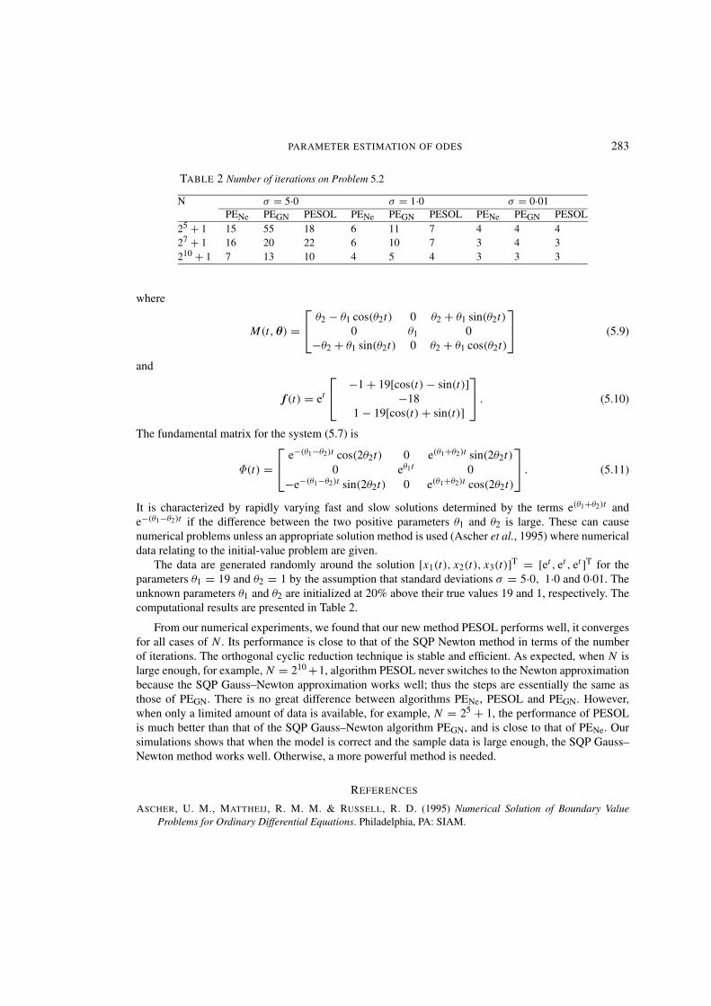
TABLE 2 Number of iterations on Problem 5.2
N σ = 5·0 σ = 1·0 σ = 0·01PENe PEGN PESOL PENe PEGN PESOL PENe PEGN PESOL
25 + 1 15 55 18 6 11 7 4 4 427 + 1 16 20 22 6 10 7 3 4 3210 + 1 7 13 10 4 5 4 3 3 3
where
M(t, θ) = θ2 − θ1 cos(θ2t) 0 θ2 + θ1 sin(θ2t)
0 θ1 0−θ2 + θ1 sin(θ2t) 0 θ2 + θ1 cos(θ2t)
(5.9)
and
f (t) = et
−1 + 19[cos(t) − sin(t)]
−181 − 19[cos(t) + sin(t)]
. (5.10)
The fundamental matrix for the system (5.7) is
Φ(t) = e−(θ1−θ2)t cos(2θ2t) 0 e(θ1+θ2)t sin(2θ2t)
0 eθ1t 0−e−(θ1−θ2)t sin(2θ2t) 0 e(θ1+θ2)t cos(2θ2t)
. (5.11)
It is characterized by rapidly varying fast and slow solutions determined by the terms e(θ1+θ2)t ande−(θ1−θ2)t if the difference between the two positive parameters θ1 and θ2 is large. These can causenumerical problems unless an appropriate solution method is used (Ascher et al., 1995) where numericaldata relating to the initial-value problem are given.
The data are generated randomly around the solution [x1(t), x2(t), x3(t)]T = [et , et , et ]T for theparameters θ1 = 19 and θ2 = 1 by the assumption that standard deviations σ = 5·0, 1·0 and 0·01. Theunknown parameters θ1 and θ2 are initialized at 20% above their true values 19 and 1, respectively. Thecomputational results are presented in Table 2.
From our numerical experiments, we found that our new method PESOL performs well, it convergesfor all cases of N . Its performance is close to that of the SQP Newton method in terms of the numberof iterations. The orthogonal cyclic reduction technique is stable and efficient. As expected, when N islarge enough, for example, N = 210 +1, algorithm PESOL never switches to the Newton approximationbecause the SQP Gauss–Newton approximation works well; thus the steps are essentially the same asthose of PEGN. There is no great difference between algorithms PENe, PESOL and PEGN. However,when only a limited amount of data is available, for example, N = 25 + 1, the performance of PESOLis much better than that of the SQP Gauss–Newton algorithm PEGN, and is close to that of PENe. Oursimulations shows that when the model is correct and the sample data is large enough, the SQP Gauss–Newton method works well. Otherwise, a more powerful method is needed.
REFERENCES
ASCHER, U. M., MATTHEIJ, R. M. M. & RUSSELL, R. D. (1995) Numerical Solution of Boundary ValueProblems for Ordinary Differential Equations. Philadelphia, PA: SIAM.
284 Z. LI ET AL.
BAER, M., HEGGER, R. & KANTZ, H. (1999) Fitting partial differential equations to space-time dynamics. Phys.Rev. E, 59, 337–342.
BARD, Y. (1974) Nonlinear Parameter Estimation. London: Academic.BIEGLER, L. T. (1998) Advances in nonlinear programming concepts for process control. J. Process Control, 8,
301–311.BOCK, H. G. (1983) Recent advances in parameter identification techniques for ODE. Numerical Treatment of
Inverse Problems in Differential and Integral Equations. (P. Deuflhard & E. Hairer, eds). Basel: Birkhauser,pp. 95–121.
BOCK, H. G. & SCHLODER, J. P. (1987) Recent progress in the development of algorithms and software forlarge scale parameter estimation problems in chemical reaction systems. Technical Report 441, Institutefur Angewandte Mathematik, Universitet Heidelberg.
BOCK, H. G., EICH, E. & SCHLODER, J. P. (1988) Numerical solution of constrained least squares boundary valueproblems in differential algebraic equations. Numerical Treatment of Differential Equations. (K. Strehmel,ed.). Leipzig: Teubner, pp. 269–280.
CHILDS, S. B. & OSBORNE, M. R. (1995) Fitting solutions of ordinary differential equations to observed data.Computational Techniques and Applications: CTAC95. (R. L. May & A. K. Easton, eds). World Scientific,Singapore, pp. 193–198.
DENNIS, J. E. & SCHNABEL, R. B. (1983) Numerical Methods for Unconstrained Optimization and NonlinearEquations. Englewood Cliffs, NJ: Prentice-Hall.
DENNIS, J. E., GAY, D. M. & WELSCH, R. E. (1981) An adaptive nonlinear least-squares algorithm. ACM Trans.Math. Software, 7, 348–368.
DEUFLHARD, P. & NOWAK, U. (1986) Efficient numerical simulation and identification of large chemical reactionsystems. Ber. Bunsenges. Phys. Chem., 90, 940–946.
EL-ALEM, M. (1995) A robust trust-region algorithm with a nonmonotonic penalty parameter scheme forconstrained optimization. SIAM J. Optim., 5, 348–378.
FLETCHER, R. (1987) Practical Methods of Optimization 2nd edn. Chichester: Wiley.FOSS, S. D. (1971) Estimates of chemical kinetic rate constants by numerical integration. Chem. Engng Sci., 26,
485–486.GALLITZENDOERFER, J. V. & BOCK, H. G. (1994) Parallel algorithms for optimization boundary value problems
in DAE. Praxisorientierte Parallelverarbeitung. (H. Langendoerfer, ed.). Munich: Hanser, pp. 156–189.HEGLAND, M. & OSBORNE, M. R. (1998) Wrap-around partitioning for block bidiagonal linear systems. IMA J.
Numer. Anal., 18, 373–383.HEMKER, P. W. (1972) Numerical methods for differential equations in system simulation and in parameter
estimation. Analysis and Simulation of Biochemical Systems. (H. C. Hemker & B. Hess. eds). pp. 59–80.IRVING, A. & DEWSON, T. (1997) Determing mixed linear-nonlinear coupled differential equations from
multivariate time series sequences. Physica D, 102, 15–36.LALEE, M., NOCEDAL, J. & PLANTENGA, T. (1998) On the implementation of an algorithm for large-scale
equality constrained optimization. SIAM J. Optim., 8, 682–706.LI, Z. F. (2000) Parameter Estimations of Ordinary Differential Equations. Ph.D. Thesis, Australian National
University, Canberra, Australia.LI, Z. F., OSBORNE, M. R. & PRVAN, T. (2002) Adaptive algorithm for constrained least squares. J. Optim.
Theory Appl., 15, 220–242.MAHDAVI-AMIRI, N. & BARTES, R. H. (1989) Constrained nonlinear least squares: an exact penalty approach
with projected structured quasi-Newton updates. ACM Trans. Math. Software, 15, 220–242.NOWAK, U. & DEUFLHARD, P. (1985) Numerical identification of selected rate constants in large chemical reaction
systems. Appl. Numer. Math., 1, 59–75.OSBORNE, M. R. (1997) Cyclic reduction, dichotomy, and the estimation of differential equations. J. Comput. Appl.
Math., 86, 271–286.

PARAMETER ESTIMATION OF ODES 285
OSBORNE, M. R. (2000) Scoring with constraints. ANZIAM J., 42, 9–25.PARLITZ, U. & MERKWIRTH, C. (2000) Prediction of spatiotemporal time series based on reconstructed local
states. Phys. Rev. Lett., 84, 1890–1893.POWELL, M. J. D. (1970) A hybrid method for nonlinear equations. Numerical Methods for Nonlinear Algebraic
Equations. (P. Rabinowitz, ed.). London: Gordan and Breach, pp. 87–114.TANARTKIT, P. & BIEGLER, L. T. (1995) Stable decomposition for dynamic optimization. Ind. Engng Chem. Res.,
34, 1253–1266.TJOA, I. B. & BIEGLER, L. T. (1991) Simultaneous solution and optimization strategies for parameter estimation
of differential-algebraic equation systems. Ind. Engng Chem. Res., 30, 376–385.WEDIN, P. A. & LINDSTROM, P. (1987) Methods and Software for Nonlinear Least Squares Problems. University
of Umea Report No. UMINF 133.87.WRIGHT, S. (1992) Stable parallel elimination for two point BVPs. SIAM J. Sci. Stat. Comput., 13, 742–764.