i

PARAMETERIZATION OF

NON-STATIONARY ACCELERATION TIME HISTORIES

Paolo Bazzurro Nicolas Luco

AIR Worldwide Corporation

Task1G00 – Final Report

December 31, 2003

ii

ABSTRACT

The main objective of this study is to investigate whether the use of “non-stationary” features of ground motion time histories in addition to more conventional elastic spectral values significantly improves the accuracy in the prediction of structural responses. The response of structures is computed here via nonlinear dynamic analysis. The 9-story SAC steel moment-resisting frame (SMRF) designed for Los Angeles conditions and three additional weaker variants are used as test cases. We have subjected these four sister buildings to a suite of 31 near-source, forward-directivity, strike-orthogonal ground motion records from four intermediate-magnitude earthquakes. Prior to the analyses, these records were compatibilized to the median elastic spectrum of the suite to simplify the statistical search for characteristics of the signal beyond the spectral values that can serve as additional response predictors. The results show that ground motion records, per-se, are neither damaging nor benign. The damageability of a record can only be measured in relation to a particular structural vibration period and specific strength. Hence, using record characteristics that do not account for the period and the strength of the structure are not likely to be “good” predictors of its response. For the structures considered here, characteristics of the velocity pulse, such as the number of half-pulses, the pulse period and the peak velocity, as well as the duration of the record do not appreciably improve the accuracy of the response estimates beyond that achieved by the use of spectral values alone. The inelastic displacement of an elastic-perfectly-plastic SDOF system with similar period and strength as the MDOF structure of interest and, more innovatively, the first “significant” peak displacement of the elastic SDOF oscillator with the same fundamental period as the MDOF structure appear to be more promising candidate predictors. The use of the latter deserves more attention in future research. Spectrum-compatible records, such as those used here, are often adopted by engineers when facing the problem of designing a new structure or assessing the response of an existing one at a site whose seismic hazard is dominated by earthquake scenarios for which real recordings are either absent or very scarce. Compatibilizing real records to match a smooth target spectrum and scaling real records to a target motion are two of the available techniques to address the lack of real recordings. The use of entirely synthetic records simulated from basic seismology principles is another option. The appropriateness of the spectrum-matching and spectrum-scaling procedures is accepted often for a lack of practical alternatives. A systematic statistical study that investigates the viability of these two approaches in terms of possible response bias and variability reduction is currently not available. We addressed this issue as well in this study. We computed the nonlinear response of SDOF and MDOF buildings of different periods and strengths subject to 31 real unscaled records, amplitude-scaled records, and spectrum-compatible records from the intermediate-magnitude, short-distance, forward-directivity scenario. Again, we consider here four variants of a 9-story steel moment-resisting frame building designed for Los Angeles conditions, as well as a suite of nonlinear SDOF systems with periods up to 4s and four strength levels. The results show that amplitude scaling tends to make the records slightly more damaging, whereas the spectrum matching approach tends to make them more benign than using real, unscaled records.

iii

Both procedures, however, reduce the record-to-record response variability and, therefore, are useful for response prediction in that they require many less records than real unscaled ones for estimating the median response with a specified level of precision. The amount of bias and variability reduction depends on the period and strength of the structure. This record-to-record variability reduction achieved by “manipulated” records is especially important for short-period structures whose response cannot be predicted with acceptable accuracy using real records unless one is prepared to carry out hundreds of nonlinear response analyses. It is worth mentioning that, rigorously speaking, the 31 records do not constitute a sample large enough to test the statistical significance of the bias at any customary level. However, the consistency of bias generated by matched or scaled records at all the periods and strength levels considered here makes for a very convincing argument.

iv

ACKNOWLEDGEMENTS

We are very grateful to Norm Abrahamson and Brian Chiou for the fruitful discussions that led to the seeding idea for this study. We also thank Walt Silva for providing us with the original records, and Nick Gregor and Norm Abrahamson for spectrum matching them. The work greatly benefited from the comments that we received at the PEER Lifelines quarterly meetings, especially from Cliff Roblee and Tom Shantz. Comments received by Allin Cornell, Helmut Krawinkler, Greg Deierlein, and Eduardo Miranda, to whom we presented preliminary results of this study, are also very much appreciated. Finally, we are extremely thankful to Dr. Norden Huang of NASA for his assistance in applying the Empirical Mode Decomposition Method to ground motion recordings. This research was made possible by the grant from the PEER Lifelines Program, Research Subagreement No. SA3592.

v

Contents Abstract ii Acknowledgements iv Table of Contents v List of Figures vii List of Tables xi 1 Overview and Organization of the Report 1 2 Decomposition of Ground Motion Records 2

2.1 Mathematical Description of the EMD Method ..................................................2 2.2 Critical Evaluation of the EMD method .............................................................5

2.2.1 Arbitrary criteria affect modes.....................................................................5 2.2.2 Sensitivity to zero padding...........................................................................6 2.2.3 Creation of artificial time-history features...................................................7 2.2.4 Tendency to produce “symmetrical” mode..................................................8 2.2.5 Differences between modes of acceleration, velocity, and displacement

time-histories................................................................................................9 2.2.6 Different modes with similar frequency contents......................................11 2.2.7 Extraction of pulses from near-source forward-directivity records...........15 2.2.8 Use of pulse characteristics for structural response prediction..................16

2.3 Conclusions ........................................................................................................17 2.4 References ..........................................................................................................17

3 Inelastic Structural Responses to Elastic-Spectrum-Matched and Amplitude-Scaled Earthquake Records 19 3.1 Introduction .......................................................................................................19 3.2 Description of the Earthquake Ground Motion Records....................................20

3.2.1 Unscaled records........................................................................................20 3.2.2 Spectrum-compatible records ....................................................................23 3.2.3 Amplitude-scaled records ..........................................................................25 3.2.4 Effects of spectrum matching on recorded ground motion time histories 26

3.3 Response of the SAC 9-story SMRF Building ..................................................29

vi

3.3.1 Description of the computer models ..........................................................29 3.3.2 Analyses results .........................................................................................31

3.4 Response of Elastic-Perfectly-Plastic SDOF Systems .......................................35 3.4.1 Description of the SDOF systems..............................................................35 3.4.2 Analyses results .........................................................................................35

3.5 Summary and Conclusions ................................................................................40 3.6 Acknowledgements ...........................................................................................42 3.7 References .........................................................................................................42

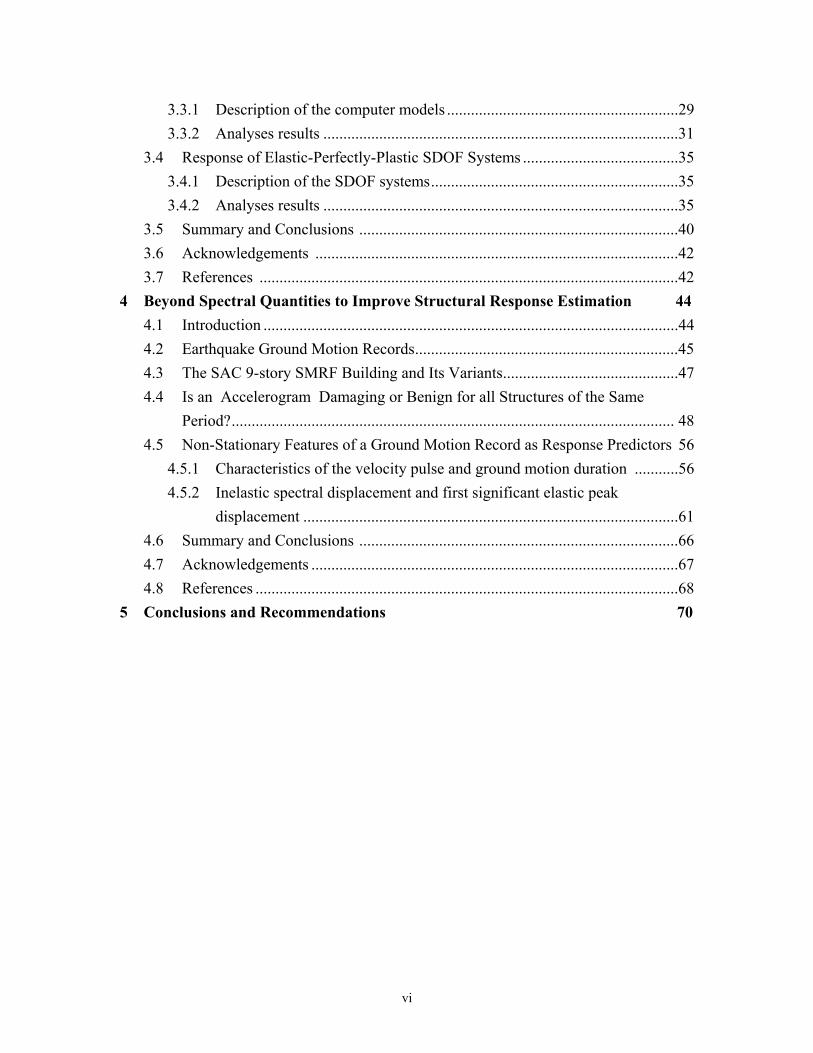
4 Beyond Spectral Quantities to Improve Structural Response Estimation 44 4.1 Introduction ........................................................................................................44 4.2 Earthquake Ground Motion Records..................................................................45 4.3 The SAC 9-story SMRF Building and Its Variants............................................47 4.4 Is an Accelerogram Damaging or Benign for all Structures of the Same

Period?............................................................................................................... 48 4.5 Non-Stationary Features of a Ground Motion Record as Response Predictors 56

4.5.1 Characteristics of the velocity pulse and ground motion duration ...........56 4.5.2 Inelastic spectral displacement and first significant elastic peak

displacement ..............................................................................................61 4.6 Summary and Conclusions ................................................................................66 4.7 Acknowledgements ............................................................................................67 4.8 References ..........................................................................................................68

5 Conclusions and Recommendations 70

vii

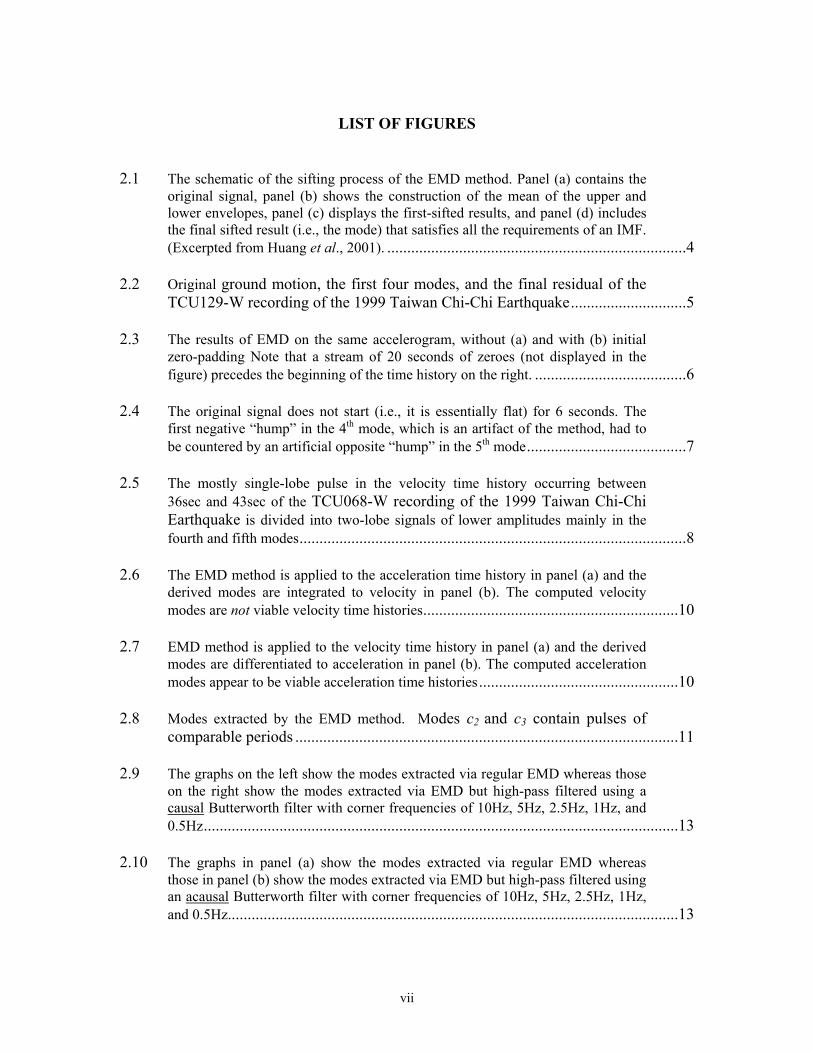
LIST OF FIGURES

2.1 The schematic of the sifting process of the EMD method. Panel (a) contains the

original signal, panel (b) shows the construction of the mean of the upper and lower envelopes, panel (c) displays the first-sifted results, and panel (d) includes the final sifted result (i.e., the mode) that satisfies all the requirements of an IMF. (Excerpted from Huang et al., 2001). ...........................................................................4

2.2 Original ground motion, the first four modes, and the final residual of the

TCU129-W recording of the 1999 Taiwan Chi-Chi Earthquake.............................5 2.3 The results of EMD on the same accelerogram, without (a) and with (b) initial

zero-padding Note that a stream of 20 seconds of zeroes (not displayed in the figure) precedes the beginning of the time history on the right. ......................................6

2.4 The original signal does not start (i.e., it is essentially flat) for 6 seconds. The

first negative “hump” in the 4th mode, which is an artifact of the method, had to be countered by an artificial opposite “hump” in the 5th mode........................................7

2.5 The mostly single-lobe pulse in the velocity time history occurring between

36sec and 43sec of the TCU068-W recording of the 1999 Taiwan Chi-Chi Earthquake is divided into two-lobe signals of lower amplitudes mainly in the fourth and fifth modes.................................................................................................8

2.6 The EMD method is applied to the acceleration time history in panel (a) and the

derived modes are integrated to velocity in panel (b). The computed velocity modes are not viable velocity time histories................................................................10

2.7 EMD method is applied to the velocity time history in panel (a) and the derived

modes are differentiated to acceleration in panel (b). The computed acceleration modes appear to be viable acceleration time histories..................................................10

2.8 Modes extracted by the EMD method. Modes c2 and c3 contain pulses of

comparable periods ................................................................................................11 2.9 The graphs on the left show the modes extracted via regular EMD whereas those

on the right show the modes extracted via EMD but high-pass filtered using a causal Butterworth filter with corner frequencies of 10Hz, 5Hz, 2.5Hz, 1Hz, and 0.5Hz.......................................................................................................................13

2.10 The graphs in panel (a) show the modes extracted via regular EMD whereas

those in panel (b) show the modes extracted via EMD but high-pass filtered using an acausal Butterworth filter with corner frequencies of 10Hz, 5Hz, 2.5Hz, 1Hz, and 0.5Hz.................................................................................................................13

viii

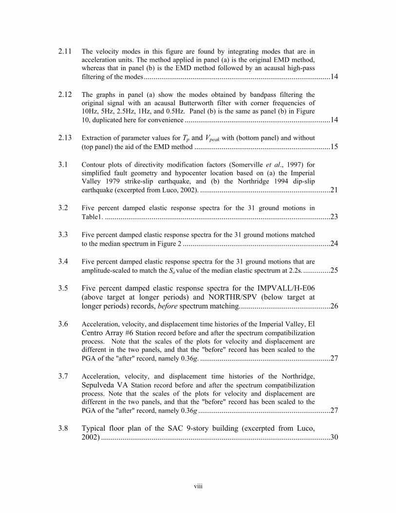
2.11 The velocity modes in this figure are found by integrating modes that are in acceleration units. The method applied in panel (a) is the original EMD method, whereas that in panel (b) is the EMD method followed by an acausal high-pass filtering of the modes................................................................................................14

2.12 The graphs in panel (a) show the modes obtained by bandpass filtering the

original signal with an acausal Butterworth filter with corner frequencies of 10Hz, 5Hz, 2.5Hz, 1Hz, and 0.5Hz. Panel (b) is the same as panel (b) in Figure 10, duplicated here for convenience ...........................................................................14

2.13 Extraction of parameter values for Tp and Vpeak with (bottom panel) and without

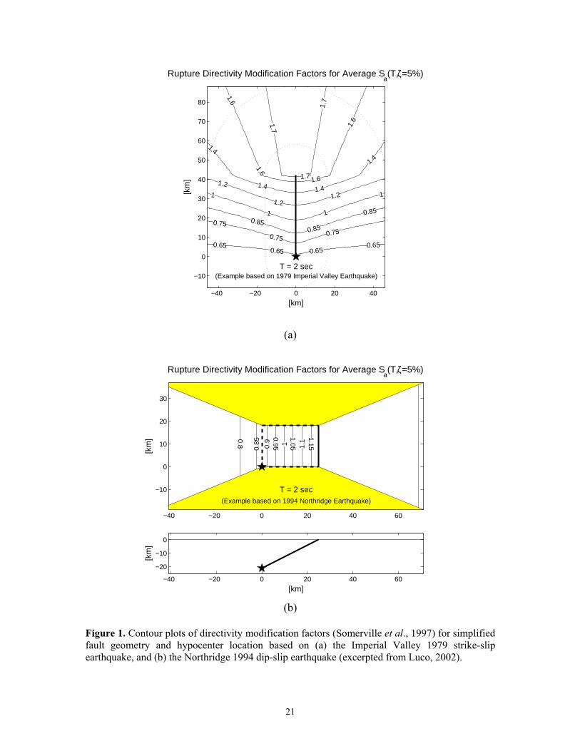
(top panel) the aid of the EMD method ......................................................................15 3.1 Contour plots of directivity modification factors (Somerville et al., 1997) for

simplified fault geometry and hypocenter location based on (a) the Imperial Valley 1979 strike-slip earthquake, and (b) the Northridge 1994 dip-slip earthquake (excerpted from Luco, 2002). ...................................................................21

3.2 Five percent damped elastic response spectra for the 31 ground motions in

Table1. ....................................................................................................................23 3.3 Five percent damped elastic response spectra for the 31 ground motions matched

to the median spectrum in Figure 2 ............................................................................24 3.4 Five percent damped elastic response spectra for the 31 ground motions that are

amplitude-scaled to match the Sa value of the median elastic spectrum at 2.2s. ..............25 3.5 Five percent damped elastic response spectra for the IMPVALL/H-E06

(above target at longer periods) and NORTHR/SPV (below target at longer periods) records, before spectrum matching...............................................26

3.6 Acceleration, velocity, and displacement time histories of the Imperial Valley, El

Centro Array #6 Station record before and after the spectrum compatibilization process. Note that the scales of the plots for velocity and displacement are different in the two panels, and that the "before" record has been scaled to the PGA of the "after" record, namely 0.36g. ...................................................................27

3.7 Acceleration, velocity, and displacement time histories of the Northridge,

Sepulveda VA Station record before and after the spectrum compatibilization process. Note that the scales of the plots for velocity and displacement are different in the two panels, and that the "before" record has been scaled to the PGA of the "after" record, namely 0.36g ....................................................................27

3.8 Typical floor plan of the SAC 9-story building (excerpted from Luco,

2002) ......................................................................................................................30

ix

3.9 Perimeter moment-resisting frame (N-S elevation) of the SAC 9-story building (excerpted from Luco, 2002) ...................................................................30

3.10 Median inelastic displacement response spectra for the four sets of SDOF

systems with strengths equal to Fy, FyR=2, Fy

R=4, and FyR=8 subject to the three

suites of 31 unscaled, amplitude-scaled, and spectrum-matched ground motions. The dashed line is at 2.2s, the fundamental period of the LA9 building ........................36

3.11 Bias due to the use of spectrum-compatible and amplitude-scaled records in lieu

of real unscaled records for the three sets of SDOF systems with strengths equal to Fy

R=2, FyR=4, and Fy

R=8. The bias is the ratio of the median displacement response spectra (Figure 10). .....................................................................................38

3.12 Variation across period of the COV of the inelastic spectral displacements for the

three sets of SDOF systems with strengths equal to FyR=2, Fy

R=4, and FyR=8,

computed using the three sets of ground motion records..............................................39 4.1 Computation of Vpeak and Tp for two spectrum-matched Northridge records

(Northr/NWH and Northr/JEN in Table 1 of Luco and Bazzurro, 2003) using both the original and the EMD-processed velocity time histories. The results from the former method are in the upper panel and those from the latter one are in the bottom panel ...................................................................................................47

4.2 Drift results of the nonlinear dynamic analyses of the four different LA9 sister

buildings, plotted as paired samples. The quantity ρ is the correlation coefficient. The three asterisks on the top margin of the graph in panels (c) and (d) represent the three collapse cases reported in Table 1. ...............................................................49

4.3 Inelastic spectral displacement results of the nonlinear dynamic analyses for the

elastic-perfectly-plastic SDOF representations of the four different LA9 sister buildings, plotted as paired samples. The quantity ρ is the correlation coefficient. Records #067 and #137 will be investigated in more detail. .........................................52

4.4 Displacement, velocity, and displacement time histories of the two spectrum-

matched records Northr/SCS (#137) and Impvall/H-E06 (#067). ...........................53 4.5 Time histories of the SDOF displacements generated by Record #137 for yield

displacements dy=30cm, dyR=2=15cm, dy

R=4=7.5cm, and dyR=8=3.75cm. The

open circles represent the maximum values over time, which are plotted in Figure 3..............................................................................................................................54

4.6 Time histories of the SDOF displacements generated by Record #067 for yield

displacements dy=30cm, dy/2=15cm, dy/4=7.5cm, and dy/8=3.75cm. The open circles represent the maximum values over time, which are plotted in Figure 3. ............55

4.7 Scatter plots of the maximum inter-story drift ratio, θmax, versus the period of

the velocity pulse, Tp, for the four 9-story building models ..................................57

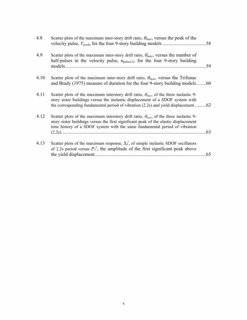
x

4.8 Scatter plots of the maximum inter-story drift ratio, θmax, versus the peak of the

velocity pulse, Vpeak, for the four 9-story building models ....................................58 4.9 Scatter plots of the maximum inter-story drift ratio, θmax, versus the number of

half-pulses in the velocity pulse, npulses/2, for the four 9-story building models ....................................................................................................................59

4.10 Scatter plots of the maximum inter-story drift ratio, θmax, versus the Trifunac

and Brady (1975) measure of duration for the four 9-story building models........60 4.11 Scatter plots of the maximum interstory drift ratio, θmax, of the three inelastic 9-

story sister buildings versus the inelastic displacement of a SDOF system with the corresponding fundamental period of vibration (2.2s) and yield displacement .........62

4.12 Scatter plots of the maximum interstory drift ratio, θmax, of the three inelastic 9-

story sister buildings versus the first significant peak of the elastic displacement time history of a SDOF system with the same fundamental period of vibration (2.2s). ......................................................................................................................63

4.13 Scatter plots of the maximum response, Sd

i, of simple inelastic SDOF oscillators of 2.2s period versus P1

e, the amplitude of the first significant peak above the yield displacement............................................................................................65

xi

LIST OF TABLES

3.1 Ground motion earthquake records used in this study..................................................22 3.2 Nonlinear dynamic drift results for the SAC LA9 building and its three weaker

sister buildings obtained using the real record dataset. The LA91/2, LA91/4, and LA91/8 buildings have approximately 1/2, 1/4, and 1/8 of the lateral strength of LA9. See Table 1 for details on the records. The numbers in italics for LA91/8 are counted statistics. .....................................................................................................32

3.3 Comparison of θmax response statistics for the LA9, LA91/2, LA91/4, and LA91/8

buildings. Sa1 is the 5%-damped spectral acceleration ath the building fundamental period of 2.2s. As in Table 2, the results for LA91/8 (in italics) are “counted statistics” due to the significant number of collapses .....................................33

4.1 Nonlinear dynamic drift results for the SAC LA9 building and its three weaker

sister buildings. The LA91/2, LA91/4, and LA91/8 buildings have approximately 1/2, 1/4, and 1/8 the lateral strength of LA9................................................................50

4.2 Measure of the record-to-record variability of θmax for the SAC LA9, LA91/2,

LA91/4, and LA91/8 buildings that is left “unexplained” by a linear regression that includes the predictor(s) in the first column. The results for LA91/8 exclude the three earthquake records in Table 1 that caused collapse. ............................................61

4.3 Measure of the record-to-record variability of θmax for the SAC LA91/2, LA91/4,

and LA91/8 buildings left “unexplained” by a linear regression model that includes the predictor(s) in the first column. The number in parenthesis represents the minimum number of records needed to estimate the median response with ±10% accuracy. The results for LA91/8 exclude the three earthquake records in Table 1 that caused collapse......................................................64

4.4 Test of the efficiency of using P1

e as a predictor of the maximum displacement response, Sd

i, of nonlinear oscillators of three vibration periods. The numbers in parentheses indicate the minimum number of records needed to achieve ±10% accuracy in the median response estimate. .................................................................................................................66

1

1 Overview and Organization of the Report

The objective of this project is to investigate whether “non-stationary” characteristics of seismograms, in addition to more conventional ground motion intensity measures (e.g., spectral values), may improve the accuracy in the prediction of structural seismic performance. Implicit in the stated scope of work is the engineering intuition that the presence of some non-stationary time-domain “features” in the ground motion signal may have a strong effect on the ability to cause damage to structures of different strengths and periods of vibration. The hope is that such features, if they exist, can be identified and predicted in terms of the basic random variables (e.g., magnitude and source-to-site distance) that define earthquake scenarios. If so, they could be coupled with more conventional ground motion intensity parameters, such as spectral quantities, to improve the accuracy in predicting structural performance. The main part of this report is organized into three parts:

1. Chapter 2. Description of the techniques used to decompose the input ground motion signal into simpler waveforms to be studied in search of the record characteristics that induce severe structural responses.

2. Chapter 3. Study of systematic differences in the inelastic response of structures to a consistent set of spectrum-matched ground motions, amplitude-scaled ground motions, and real, unscaled motions.

3. Chapter 4. Search beyond spectral quantities for ground motion intensity measures that may improve structural response estimation, with an emphasis on time-domain features.

The report is concluded with Chapter 5 that summarizes the findings and provides recommendations for future follow-up studies. Note that Chapters 3 and 4 are written as self-contained units, as they represent articles to be submitted for journal publications. This choice of presentation, however, has caused some repetitions for which we apologize to the readers.

2

2 Decomposition of Ground Motion Records

Ground motions are highly non-stationary signals that, usually, possess a very complex structure. To investigate whether embedded in signals there exist any time-domain features that are responsible for the effectiveness in creating structural damage, we used a simple but adaptive processing technique known as the Empirical Mode Decomposition (EMD) method (Huang et al., 1998). This technique is, by design, applicable to nonstationary time histories. EMD is recommended as the first step of a Hilbert Spectrum Analysis, a procedure that provides information on how the energy content of the signal evolves over time. In this study, however, we limited ourselves to the use of the EMD technique. Note that, given its intrinsic assumption of stationarity, the more familiar Fourier transform that decomposes a signal into harmonics is, strictly speaking, not ideal for tackling this problem. The EMD is an algorithm that decomposes a complicated time history into a finite and often small number of “intrinsic mode functions” (IMF’s) or “modes” for short, whose characteristics (and visual appearance) are much simpler than those of the original signal. The modes have several properties that make their use very appealing (for details, see Huang et al., 1998), but in this study the most important one is that they extract the characteristics of the signal at different time scales. Similar in concept to the sines and cosines of the Fourier Spectrum, the modes can serve as a nearly orthogonal basis for reconstructing the original signal within a specified tolerance, which is known. The modes, however, unlike the sinusoidal waves used in the Fourier transform, can have both amplitude and frequency modulations. The EMD method is completely general and can be applied to any type of signal. Example applications include ocean and wave-tank-generated waves, ocean surface elevation, wind-generated turbulence, and ground motions (e.g., Huang et al., 1998, 1999, and 2001; Loh et al. 2001). The hope for this project is that the characteristics of these modes computed for several ground motions from the same scenario (e.g., same magnitude and distance range) will reveal some meaningful systematic pattern across records that could be used for response prediction purposes. The damage effectiveness of such modes, and of the original ground motions, is tested by evaluating the responses of single-degree-of-freedom (SDOF) oscillators of different periods and realistic structures such as the 9-story steel moment-resisting frame designed for Los Angeles conditions as part of Phase II of the SAC Steel Project (FEMA 355C, 2000).

2.1 Mathematical Description of the EMD Method The EMD method, in its original definition (Huang et al., 1998), can be summarized as follows:

)()()(1

trtctX n

n

jj += ∑

=

3

where X(t) is the signal, cj(t) is the j-th of n modes (or IMF’s), and rn(t) is the residual time history left over at the end of the procedure. The modes are extracted via a “sifting” process that is iterative in nature and whose rules are subjectively defined on the basis of the experience gained in dealing with different real-life signals. The two main purposes of the sifting process are to remove “riding” waves (starting from high-frequency waves down to longer period ones), and to make the wave profile more symmetrical. It is called sifting because the signal is subject to less and less refined “sieves,” each one of which separates the finest (namely, highest-frequency) mode from the rest of the signal. In words, the sifting procedure consists of removing repeatedly from the signal, X(t), the mean of the upper and lower envelopes curves until a specified criterion stops the sifting, delivering the first mode, c1(t), and a residual time history, r1(t). The stopping criterion states that within the data range the number of zero crossings and extrema should be equal, or differ by only one. This original criterion was updated in Huang et al., 2001, to require that the number of zero crossings and extrema be equal for three consecutive siftings. Huang, in a personal communication, suggested that we further increase to five the number of siftings. In general, c1(t) contains the finest-scale, that is the shortest-frequency, component of the signal. The second round of sifting follows the same rules, but it is applied to r1(t) rather than to X(t). The sifting process is repeated as many times as needed for the signal at hand. The total number of times, called n in Equation 1, is reached when the residual time history either has amplitudes that are too small to generate any appreciable consequence for the considered application, or has become a monotonic function from which no IMF can be extracted. At that point the residual time history, which takes on the name of rn(t), represents the difference between the original signal and the addition of all the extracted modes. More formally, the following steps summarize the version of the EMD procedure that we applied in this study:

• Each mode ci(t) is computed by a procedure that contains several rounds of sifting.

• Call m1(t), m11(t), m12(t), … the mean of the lower and upper envelope curves of X(t), h1(t), h11(t), h12(t), … The quantities h1(t) and h11(t) are the first and second sifted components of the signal and are computed as specified below.

• Five-step sifting procedure: 1) )()()( 11 thtmtX =− 2) )()()( 11111 thtmth =− …………… 3) )()( 11 tcth k = . Stop procedure when five consecutive siftings give the same number of zero-crossings and extrema. 4) )()()( 11 trtctX =− 5) Replace X(t) with r1(t) in Step 1 and repeat Steps 1-5.

4

• Stop sifting when the final residual, rn(t), is either too small to be of any practical interest, or the when it has become a monotonic function.

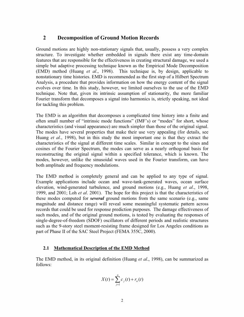
The effects on the first six seconds of TCU129-W recording of the 1999 Taiwan Chi-Chi Earthquake of the sifting procedure leading to the first mode are shown in Figure 1. Figure 2 instead displays all the modes that were extracted from the same recording before the maximum amplitude of the final residual (last panel) dropped below the arbitrarily selected threshold value of 0.05g. It is apparent that the high- frequency part of the signal tends to be removed by the first few modes.

Figure 1: The schematic of the sifting process of the EMD method. Panel (a) contains the original signal, panel (b) shows the construction of the mean of the upper and lower envelopes, panel (c) displays the first-sifted results, and panel (d) includes the final sifted result (i.e., the mode) that satisfies all the requirements of an IMF. (Excerpted from Huang et al., 2001).

5

-101

X(t)

-0.5

0

0.5

c 1

-0.5

0

0.5c 2

-0.5

0

0.5

c 3

-0.5

0

0.5

c 4

20 30 40 50 60 70 80 90-0.5

0

0.5

r 4

t

Figure 2: Original ground motion, the first four modes, and the final residual of the TCU129-W recording of the 1999 Taiwan Chi-Chi Earthquake.

2.2 Critical Evaluation of the EMD method We have applied the EMD procedure to about one hundred ground motion recordings. This data set includes the 60 ground motions developed for Los Angeles by the SAC Steel Project, a few fault-normal and fault-parallel records from both the Landers and the Chi-Chi earthquakes, and 31 near-source, normal component records (see Table 1 in Section 3) that were spectrum compatibilized to their median elastic response spectrum by Dr. Abrahamson of PG&E. The application of the EMD to such cases has identified some aspects of this methodology that are potentially problematic for the scope of this study. Huang and his co-workers in their original articles also recognized some of these drawbacks, some of which are methodological and some which are application-dependent. The comments in the next subsections are explained with the aid of specific examples. The conclusions, however, are made from the analysis of many recordings and not just of those displayed in the figures that follow.

2.2.1 Arbitrary criteria affect modes In this study we intended to use EMD as a screening tool for identifying common time- domain features in different ground motions that may be responsible for their

6

effectiveness in inducing severe structural responses. Our hope was that a limited number of similar modes (one, in the limit) from different ground motions would contain one or more common features that were easily identifiable as causing large responses. The criteria that control the sifting process (e.g., the stopping criteria to be adopted during sifting, the mathematical nature of the envelope curves, the length of pre- and post-record zero-padding), however, do have a strong influence on the modes that are extracted from a time history. For example, a particular time feature (e.g., a pulse) can appear in one mode if one set of rules is adopted, or be split into two consecutive modes if another set is used instead. Since the criteria for sifting are inherently subjective, being derived from experience rather than having a mathematical or physical basis, also the modes that originate from their application become somewhat subjective as well. Some examples of this are treated in more details in the following subsections.

2.2.2 Sensitivity to zero padding Removing zeroes from the beginning of a time history changes the appearance of some of the modes. This is an undesirable feature of the method. Figure 3 shows the first four modes extracted from the same accelerogram, the TCU129-W recording of the 1999 Taiwan Chi-Chi Earthquake, without and with 20 seconds of zeroes before the beginning of the real signal. The difference between corresponding pairs of modes is evident. We expect that zero-padding the tail of a signal may cause a similar difference in the EMD-extracted modes.

-1

0

1

X(t)

Chi-Chi/Station129/TCU129-W

-0.5

0

0.5

c 1

-0.50

0.5

c 2

-0.5

0

0.5

c 3

0 10 20 30 40 50 60 70-0.2

0

0.2

c 4

t

-1

0

1

X(t)

Chi-Chi/Station129/TCU129-W

-0.5

0

0.5

c 1

-0.50

0.5

c 2

-0.5

0

0.5

c 3

20 30 40 50 60 70 80 90-0.2

0

0.2

c 4

t

(a) (b) Figure 3: The results of EMD on the same accelerogram, without (a) and with (b) initial zero-padding Note that a stream of 20 seconds of zeroes (not displayed in the figure) precedes the beginning of the time history on the right.

7

2.2.3 Creation of artificial time-history features

The type of lower and upper envelope curves that touch the extrema of the process carries some consequences on the form of the extracted IMF’s. The type of envelope suggested by the authors of the method is a cubic spline. The spline curve, however, tends to overshoot and undershoot the real signal, creating an undesirable source of noise that can be significant at times. This problem is also clearly recognized in studies by the developers of this method. One clear example of this problem is shown in Figure 4. No signal of any engineering significance is present in the first six seconds of the time history. The EMD method, however, artificially adds before six seconds a negative “hump” in the 4th IMF and a positive “hump” in the 5th IMF, to counteract the former. The addition of both, of course, has a null net effect and does not hinder the recover of the original time history. However, if one needs to use some of the modes and not the original signal, these artifacts of the method are sources of undesirable noise.

-0.50

0.5

A(t)

SAC LA40 (simulated)

-0.50

0.5

c 1

-0.50

0.5

c 2

-0.50

0.5

c 3

-0.50

0.5

c 4

0 5 10 15 20 25 30-0.5

00.5

c 5

t

Figure 4: The original signal does not start (i.e., it is essentially flat) for 6 seconds. The first negative “hump” in the 4th mode, which is an artifact of the method, had to be countered by an artificial opposite “hump” in the 5th mode.

8

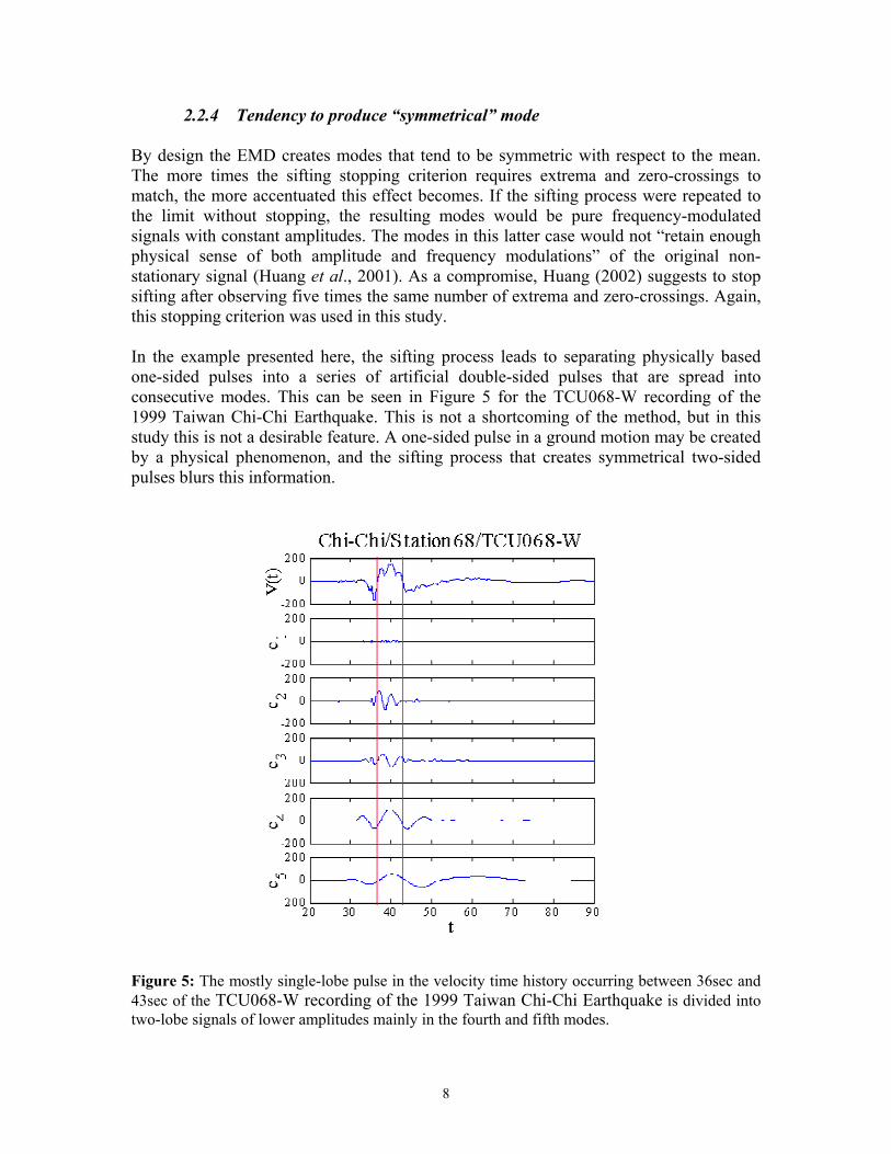
2.2.4 Tendency to produce “symmetrical” mode By design the EMD creates modes that tend to be symmetric with respect to the mean. The more times the sifting stopping criterion requires extrema and zero-crossings to match, the more accentuated this effect becomes. If the sifting process were repeated to the limit without stopping, the resulting modes would be pure frequency-modulated signals with constant amplitudes. The modes in this latter case would not “retain enough physical sense of both amplitude and frequency modulations” of the original non-stationary signal (Huang et al., 2001). As a compromise, Huang (2002) suggests to stop sifting after observing five times the same number of extrema and zero-crossings. Again, this stopping criterion was used in this study. In the example presented here, the sifting process leads to separating physically based one-sided pulses into a series of artificial double-sided pulses that are spread into consecutive modes. This can be seen in Figure 5 for the TCU068-W recording of the 1999 Taiwan Chi-Chi Earthquake. This is not a shortcoming of the method, but in this study this is not a desirable feature. A one-sided pulse in a ground motion may be created by a physical phenomenon, and the sifting process that creates symmetrical two-sided pulses blurs this information.

Figure 5: The mostly single-lobe pulse in the velocity time history occurring between 36sec and 43sec of the TCU068-W recording of the 1999 Taiwan Chi-Chi Earthquake is divided into two-lobe signals of lower amplitudes mainly in the fourth and fifth modes.

9

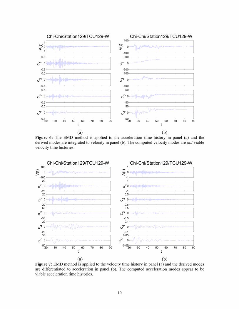
2.2.5 Differences between modes of acceleration, velocity, and displacement time-histories

To test the robustness of the EMD method for the application at hand, we applied it to acceleration, velocity, and displacement time histories of the same recordings and checked for “seismological consistency” of the computed modes. The consistency was checked in two ways:

a) We applied the EMD method to, for example, an accelerogram and then integrated the extracted modes once and twice to obtain modes for velocity and displacement, respectively. These modes were then inspected to evaluate whether they were “plausible” ground motion signals from a seismological point of view. b) We compared the modes computed via integration from the acceleration modes with the IMF’s obtained directly via EMD on the time histories of velocity and displacement

Similarly, we repeated (a) and (b) with velocity and displacement time histories. Figure 6 shows the application of EMD to the 1999 Taiwan Chi-Chi TCU129-W accelerogram. The modes on the left were then integrated to obtain corresponding modes in velocity, which were added together to obtain a velocity time history (the right uppermost panel). The modes derived via integration in the right panel do not resemble plausible velocity time histories of a real ground motion. The original velocity time history, however, is fully recovered by adding all the modes. This is to be expected given that integration (like differentiation) is a linear operation. Similarly, we repeated the same steps starting from the velocity time history of the same recording and applied the EMD procedure to obtain the modes shown in panel (a) of Figure 7. Such velocity modes were then differentiated to obtain modes in acceleration units. This operation provided IMF’s that visually resemble plausible acceleration signals, as can be appreciated from Figure 7, panel (b). When added, the derived acceleration modes recover the original accelerogram, as expected. Although not shown here, we also examined the EMD method applied to displacement time histories whose EMD-derived modes were differentiated once and twice. The results indicated that the differentiation to velocity created modes that, considered separately, did not resemble real ground motion velocity time histories. It is implicit in the previous discussion that the modes obtained via EMD on a signal (e.g., ground motion velocity) are different from those found via integration or differentiation of the corresponding EMD-based modes derived from other quantities (e.g., ground motion acceleration and displacement). The graphs in panel (b) of both Figures 6 and 7 clearly show the difference. This conclusion comes to no surprise given that the EMD is a nonlinear operation.

10

-101

A(t)

Chi-Chi/Station129/TCU129-W

-0.5

0

0.5

c 1

-0.5

0

0.5

c 2

-0.5

0

0.5

c 3

20 30 40 50 60 70 80 90-0.5

0

0.5

c 4

t

-100

0

100

V(t)

Chi-Chi/Station129/TCU129-W

-500

0

500

c 1

-100

0

100

c 2

-50

0

50

c 320 30 40 50 60 70 80 90

-50

0

50

c 4t

(a) (b) Figure 6: The EMD method is applied to the acceleration time history in panel (a) and the derived modes are integrated to velocity in panel (b). The computed velocity modes are not viable velocity time histories.

-100

0

100

V(t)

Chi-Chi/Station129/TCU129-W

-20

0

20

c 1

-20

0

20

c 2

-50

0

50

c 3

-20

0

20

c 4

20 30 40 50 60 70 80 90-50

0

50

c 5

t

-1

0

1

A(t)

Chi-Chi/Station129/TCU129-W

-1

0

1

c 1

-0.5

0

0.5

c 2

-0.5

0

0.5

c 3

-0.1

0

0.1

c 4

20 30 40 50 60 70 80 90-0.05

0

0.05

c 5

t

(a) (b) Figure 7: EMD method is applied to the velocity time history in panel (a) and the derived modes are differentiated to acceleration in panel (b). The computed acceleration modes appear to be viable acceleration time histories.

11

In conclusion, for the purposes of this study the EMD method seems to work better when applied to a velocity signal rather than to an acceleration or a displacement time history. When used in conjunction with acceleration or displacement time histories, the EMD method produces some undesirable features when one integrates or differentiates the derived modes.

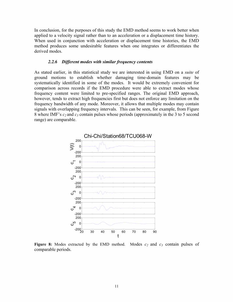
2.2.6 Different modes with similar frequency contents

As stated earlier, in this statistical study we are interested in using EMD on a suite of ground motions to establish whether damaging time-domain features may be systematically identified in some of the modes. It would be extremely convenient for comparison across records if the EMD procedure were able to extract modes whose frequency content were limited to pre-specified ranges. The original EMD approach, however, tends to extract high frequencies first but does not enforce any limitation on the frequency bandwidth of any mode. Moreover, it allows that multiple modes may contain signals with overlapping frequency intervals. This can be seen, for example, from Figure 8 where IMF’s c2 and c3 contain pulses whose periods (approximately in the 3 to 5 second range) are comparable.

-200

0

200

V(t)

Chi-Chi/Station68/TCU068-W

-200

0

200

c 1

-200

0

200

c 2

-200

0

200

c 3

-200

0

200

c 4

20 30 40 50 60 70 80 90-200

0

200

c 5

t

Figure 8: Modes extracted by the EMD method. Modes c2 and c3 contain pulses of comparable periods.

12

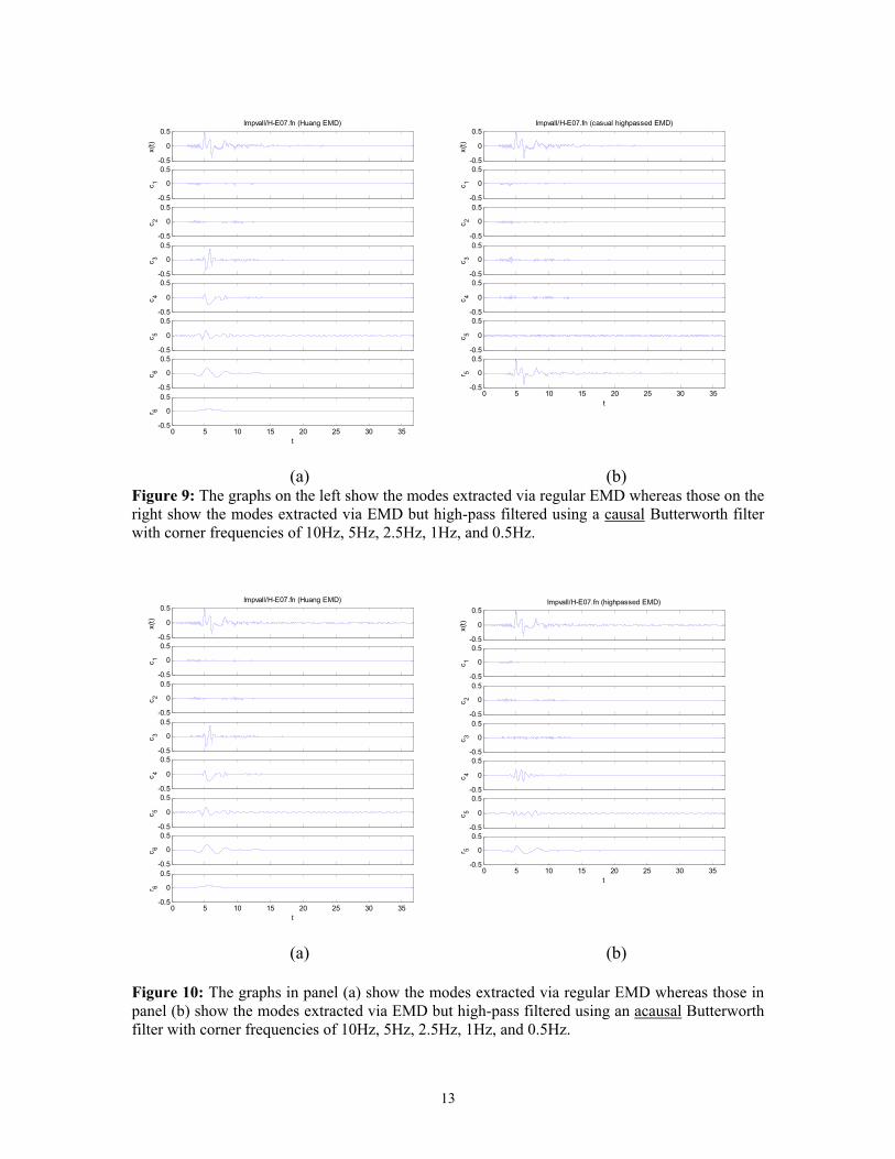
To alleviate these problems, we tested two variants of the original EMD method. The first one involves high-pass filtering the first five modes extracted from EMD with a causal1 Butterworth filter with corner frequencies set to 10Hz, 5Hz, 2.5Hz, 1Hz and 0.5Hz, respectively. Of course, the part of each IMF that is filtered out is put back into the leftover signal that serves as the input for the extraction of the following mode. After five modes are extracted the process stops and the sixth mode is considered as the residual. The second EMD variant differs from the first one only in the characteristics of the Butterworth filter, which is instead acausal2. The main difference between the two alternatives is that the causal filter distorts the phases of the original signal while the acausal filter produces a sequence that has precise zero-phase distortion and double the filter order. The effects of applying the causal Butterworth filter (with high-pass corner frequencies as specified above) to the normal component of the Imperial Valley Earthquake recorded at Station H-E07 is shown in the right panel of Figure 9. The left panel displays the modes obtained via EMD without applying any high-pass filtering (namely, the original EMD procedure). The phase-distortion introduced by the causal filter prevents the EMD procedure from extracting meaningful modes and the residual contains almost an exact copy of the original signal. The use of acausal filtering instead is shown in the right panel of Figure 10. In this case the EMD procedure with high-pass filtering of the modes creates IMF’s that have content in the desired frequency bandwidths. For the purposes of this study, this represents an improvement over the original EMD procedure. The use of an acausal filter applied to the EMD-based modes removes two sources of concerns discussed in Subsections 2.2.3 and 2.2.5. In particular, spurious artifacts of the EMD method, such as the opposite humps introduced before the beginning of the signal, did not appear after the application of the acausal filter to the modes. Also, the modes that this modified EMD method produces when applied to acceleration time histories integrate to modes in units of velocity that resemble plausible ground motion velocity time histories. The latter can be seen in Figure 11 that compares the velocity modes integrated from acceleration modes obtained a) with the original EMD method and b) with the EMD plus acausal high-pass filter. It is worthwhile to note that one could have obtained modes similar to those in panel (b) of Figure 10 by simply applying an acausal Butterworth bandpass filter to the original signal without the use of EMD. This is shown in Figure 12, which presents the modes from bandpass filtering the original signal side-by-side with those obtained by applying an acausal high-pass filter to the modes extracted via EMD (same as panel (b) of Figure 10). Although not shown here, the acausal bandpass filter without EMD method also possesses the same property that the acceleration modes integrate to meaningful velocity modes.

1 For causal here we mean that the signal is processed only in the forward direction. 2 For acausal we mean that the filter is applied in both forward and reverse directions. After filtering the signal in the forward direction, the filtered sequence is reversed and run back through the filter.

13

-0.5

0

0.5

x(t)

Impvall/H-E07.fn (Huang EMD)

-0.5

0

0.5

c 1

-0.5

0

0.5

c 2

-0.5

0

0.5

c 3

-0.5

0

0.5

c 4

-0.5

0

0.5

c 5

-0.5

0

0.5

c 6

0 5 10 15 20 25 30 35-0.5

0

0.5

r 6

t

-0.5

0

0.5

x(t)

Impvall/H-E07.fn (casual highpassed EMD)

-0.5

0

0.5

c 1

-0.5

0

0.5

c 2

-0.5

0

0.5

c 3

-0.5

0

0.5

c 4

-0.5

0

0.5

c 5

0 5 10 15 20 25 30 35-0.5

0

0.5

r 5

t

(a) (b) Figure 9: The graphs on the left show the modes extracted via regular EMD whereas those on the right show the modes extracted via EMD but high-pass filtered using a causal Butterworth filter with corner frequencies of 10Hz, 5Hz, 2.5Hz, 1Hz, and 0.5Hz.

-0.5

0

0.5

x(t)

Impvall/H-E07.fn (Huang EMD)

-0.5

0

0.5

c 1

-0.5

0

0.5

c 2

-0.5

0

0.5

c 3

-0.5

0

0.5

c 4

-0.5

0

0.5

c 5

-0.5

0

0.5

c 6

0 5 10 15 20 25 30 35-0.5

0

0.5

r 6

t

-0.5

0

0.5

x(t)

Impvall/H-E07.fn (highpassed EMD)

-0.5

0

0.5

c 1

-0.5

0

0.5

c 2

-0.5

0

0.5

c 3

-0.5

0

0.5

c 4

-0.5

0

0.5

c 5

0 5 10 15 20 25 30 35-0.5

0

0.5

r 5

t

(a) (b)

Figure 10: The graphs in panel (a) show the modes extracted via regular EMD whereas those in panel (b) show the modes extracted via EMD but high-pass filtered using an acausal Butterworth filter with corner frequencies of 10Hz, 5Hz, 2.5Hz, 1Hz, and 0.5Hz.

14

-200

0

200

x(t)

Impvall/H-E07.fn (Huang EMD integrated)

-200

0

200

c 1

-200

0

200

c 2

-200

0

200

c 3

-200

0

200

c 4

-200

0

200

c 5

-200

0

200

c 6

0 5 10 15 20 25 30 35-200

0

200

r 6

t

-200

0

200

x(t)

Impvall/H-E07.fn (highpassed EMD integrated)

-200

0

200

c 1

-200

0

200

c 2

-200

0

200

c 3

-200

0

200

c 4

-200

0

200

c 5

0 5 10 15 20 25 30 35-200

0

200

r 5

t

(a) (b) Figure 11: The velocity modes in this figure are found by integrating modes that are in acceleration units. The method applied in panel (a) is the original EMD method, whereas that in panel (b) is the EMD method followed by an acausal high-pass filtering of the modes.

-0.5

0

0.5

x(t)

Impvall/H-E07.fn (bandpassed)

-0.5

0

0.5

c 1

-0.5

0

0.5

c 2

-0.5

0

0.5

c 3

-0.5

0

0.5

c 4

-0.5

0

0.5

c 5

0 5 10 15 20 25 30 35-0.5

0

0.5

r 5

t

-0.5

0

0.5

x(t)

Impvall/H-E07.fn (highpassed EMD)

-0.5

0

0.5

c 1

-0.5

0

0.5

c 2

-0.5

0

0.5

c 3

-0.5

0

0.5

c 4

-0.5

0

0.5

c 5

0 5 10 15 20 25 30 35-0.5

0

0.5

r 5

t

(a) (b) Figure 12: The graphs in panel (a) show the modes obtained by bandpass filtering the original signal with an acausal Butterworth filter with corner frequencies of 10Hz, 5Hz, 2.5Hz, 1Hz, and 0.5Hz. Panel (b) is the same as panel (b) in Figure 10, duplicated here for convenience.

15

2.2.7 Extraction of pulses from near-source forward-directivity records

The EMD algorithm did prove useful in extracting “pulse” parameters (period, Tp, number of half-cycles, npulses/2, peak velocity, Vpeak) from the normal component of near-source forward-directivity records. Loh et al. (2001) also recognized the usefulness of EMD in isolating pulses within such records. The use of EMD can help in removing some ambiguity in the extraction of Tp, npulses/2, and Vpeak, values to be used as additional ground motion parameters in structural response prediction studies. One example is shown in Figure 13, where the values obtained from the original velocity time history (top panel) are compared with those from the EMD residual after the removal of the first three modes. The double-sided pulse in r3 is much clearer after the removal of the high-frequency riding waves by means of the EMD method.

Figure 13: Extraction of parameter values for Tp and Vpeak with (bottom panel) and without (top panel) the aid of the EMD method. To demonstrate that the EMD-extracted pulses and their parametric values are consistent with the original signals, we computed the nonlinear structural response of the 9-story steel moment-resisting frame (SMRF) building designed for Los Angeles conditions as part of the SAC Steel Project (see Section 3 of this report for more details) for a subset of 31 near-source, pulse-like forward-directivity records (see Table 1 in Section 3). The response was computed twice for each record, the first time using the entire signal and the second time using only the EMD-extracted residual that contains the pulse. This pulse was found by stopping the EMD procedure when there were no riding waves on the lobe surrounding the peak of the residual (i.e., Vpeak). It should be noted that the 31 records were compatibilized to the median elastic spectrum of the suite prior to using

16

them as input to the nonlinear dynamic analyses. The reason for not employing the original ground motions will be clear in the next subsection. It is not expected, however, that the spectrum compatibilization process invalidates the conclusions that follow. The results for the randomly selected subset of 13 records showed that, on average, the maximum interstory drift ratio across the height of the building (a widely-used measure of the collapse potential of SMRF buildings) obtained using only the pulse as the input ground motion is lower by only 10% than that obtained using the entire signal (i.e., medians of 0.0243 vs. 0.0269). These findings confirm that:

• The pulses extracted by EMD, and consequently, the parameters that characterize the pulse (Tp, npulses/2, and Vpeak) are meaningful. We will use this approach in Sections 3 and 4 of this report to extract pulse parameters for structural response prediction purposes.

• The pulse essentially captures the potential of forward-directivity normal- component records to induce severe structural responses of moderate-to-long period structures. Higher-frequency riding waves do not significantly affect the structural response of these structures subject to such near-source records.

The latter item above is discussed in more detail in the next subsection.

2.2.8 Use of pulse characteristics for structural response prediction The median responses of the SAC 9-story building to both near-source forward directivity ground motions and to single EMD-derived modes extracted from each of them are statistically close. This implies that, at least for this case (namely, this set of records and this structure), the modes containing the pulses are the time domain features that we set out to find. The pulses, in fact, are responsible for the damage effectiveness of these records. The other modes that contain higher frequencies can essentially be neglected when computing the response of moderate-to-long period structures. This is hardly a novel result, however. What is novel is the statistical analysis that follows. Given these premises, the characteristics of the pulse considered here, that is the number of half-pulses, npulses/2, the pulse period, Tp, and the peak velocity, Vpeak, should, at least intuitively, bear a correlation with the severity of the induced structural response. To avoid confusing the issue at stake with unnecessary statistical analyses, as mentioned before we have spectrum compatibilized the near-source records prior to using them as input for the response analyses and for the extraction of modes by the EMD procedure. The compatibilization makes all the records share the same elastic spectrum, that is it makes all of them equally damaging at least in an elastic-response sense. The original 5%-damped elastic spectra of the 31 records before compatibilization and their median spectrum are displayed in Figure 2 of Section 3. Figures 7, 8, and 9 in Section 4 (not repeated here for conciseness) show that the expected correlation with Tp, Vpeak, and npulses/2 is virtually absent. This means that knowing these characteristics of the pulses once that the elastic spectral quantities of a

17

ground motion are known does not improve the accuracy of the response estimates. More formally, the record-to-record variability of the response does not decrease once a regression analyses is performed with a model containing any combination of predictor variables selected among npulses/2, Tp, and Vpeak. These results were confirmed for four variants of the SAC 9-story building that encompass a wide range of strength levels and degrees of response nonlinearity. In summary, on average the EMD-derived pulses alone essentially account for the entire structural response of the SAC 9-story building. Therefore, the sought-after non-stationary time-domain feature that is responsible for the record damage effectiveness is, in this case, the pulse itself (or, better, a simplified version of it). The pulse parameters, however, are not useful predictors of responses when used in addition to the elastic response spectrum.

2.3 Conclusions The initial part of this study showed that EMD, despite some drawbacks, has proven to be a useful methodology to extract pulses from near-source, forward-directivity, normal- component records. Pulses are the non-stationary time features responsible for the damage effectiveness of these records to the moderately long period structures considered. The knowledge of pulse characteristics, however, does not appreciably improve the accuracy of structural response estimates beyond that achieved by using only more conventional ground motion intensity measures, namely spectral values. The results included in the sections to come will also demonstrate that the initial goal of this project was too ambitious. There is no time-domain nonstationary feature to be found in a ground motion signal that makes it either very damaging or very benign to structures of different periods and strengths. As shown in Section 4, there is only a weak correlation between the nonlinear response caused by the same record to strong and weak structures with the same initial fundamental period of vibration. Hence, the damage potential of a record is a meaningful concept only when addressed in relation to a structure of a given period and strength.

2.4 References .

Federal Emergency Management Agency (FEMA) (2000). ``State of the Art Report on System Performance of Steel Moment Frames Subject to Ground Shaking”, FEMA 355C, September 2000. Huang, N.E., Shen, Z., and S.R. Long (1999). “A New View of Nonlinear Water Waves: the Hilbert Spectrum”, Annu. Rev. Fluid Mech., Vol. 31, pp. 417-457. Huang, N.E., Shen, Z., Long, S.R., Wu, M.C., Shih, H.H., Zheng, Q., Yen, N-C., Tung, C.C., and H.H. Liu (1998). “The Empirical Mode Decomposition and the Hilbert

18

Spectrum for Nonlinear and Non-Stationary Time Series Analysis”, Proc. Of the Royal Society of London, Vol. 454, pp. 903-995, London, UK. Huang, N.E., Chern, C.C., Huang, K., Salvino, L.W., Long, S.R., and K.L. Fan (2001) ”A New Spectral Representation of Earthquake Data: Hilbert Spectral Analysis of Station TCU129, Chi-Chi, Taiwan, 21 September 1999”, B.S.S.A., Vol. 91, No. 5, pp. 1310-1338, October. Huang, N.E. (2002). Personal Communication, Bethesda, MD, October. Loh, C-H., Wu, T-C., and N.E. Huang (2001). ”Application of the Empirical Mode Decomposition-Hilbert Spectrum Method to Identify Near-Fault Ground-Motion Characteristics and Structural Responses”, B.S.S.A., Vol. 91, No.5, pp. 1339-1357, October.

19

3 Inelastic Structural Responses to Elastic-Spectrum-Matched

and Amplitude-Scaled Earthquake Records Abstract: Engineers often face the problem of designing a new structure or assessing the response of an existing one at a site whose seismic hazard is dominated by earthquake scenarios for which real recordings are either absent or very scarce. Scaling real records to a target motion or compatibilizing real records to match a smooth target spectrum are two techniques that are used in practice to address this problem. The appropriateness of such procedures is accepted often for a lack of practical alternatives. A systematic statistical study that investigates the viability of these two approaches in terms of possible response bias and variability reduction is currently not available. This article intends to study the nonlinear response of SDOF and MDOF buildings of different periods and strengths subject to real unscaled records, amplitude-scaled records, and spectrum-compatible records from an intermediate-magnitude, short-distance, forward-directivity scenario. We consider here four variants of a 9-story steel moment-resisting frame building designed for Los Angeles conditions, and a suite of nonlinear SDOF systems with periods up to 4s and four strength levels. The results show that amplitude scaling tends to make the records slightly more damaging, whereas the spectrum matching approach tends to make them more benign than real, unscaled records. Both procedures, however, reduce the record-to-record response variability and, therefore, are useful for response prediction in that they require many less records than real unscaled ones for estimating the median response with the same level of precision. The amount of bias and variability reduction depends on the period and strength of the structure.

3.1 Introduction Engineers have used over the years several different analysis techniques to estimate the seismic performance of new or existing structures located at a specific site. Among the different approaches, nonlinear dynamic analysis is generally believed to provide the most realistic predictions of structural response induced by earthquake ground motions. The input ground motions to such analyses are usually selected to be either representative of earthquake scenarios that control the site hazard, or consistent with predefined, “smooth” target elastic response spectra. In both cases, the desired input ground motions are usually very intense. The scarcity of real recordings with the right characteristics has often forced practitioners to “manipulate” real accelerograms. The manipulation involves scaling the input time histories to the desired intensity level or using them as “seeds” to be spectrum-matched to the given target. Whatever the technique adopted, the accuracy of the prediction generally depends on the number of response analyses performed and on the characteristics of the necessarily limited suite of seismograms selected for such analyses. In the last decade researchers have suggested that the use of amplitude-scaled records and spectrum-matched records is not only legitimate, but also useful, because it limits the number of nonlinear dynamic analysis runs compared to the use of unscaled, real records without compromising the accuracy of the estimation (e.g., Carballo and Cornell, 2000). In this article we take a close look at the use of both amplitude-scaled records and spectrum-matched records for structural response estimation. In particular, we consider a suite of near-source records

20

from intermediate magnitude events that are altered in both ways and we statistically compare the structural responses generated by these two sets with those of the original recordings. The primary focus of our search is not on the reduction in response variability, a topic that has been studied before, but on the possible systematic bias that these techniques may induce. To give a large breadth to the results, we consider both a Multi-Degree-of-Freedom (MDOF) 9-story steel moment-resisting frame (SMRF) structure and a large set of inelastic Single-Degree-of-Freedom (SDOF) systems with different periods and strengths. Finally, note that the use of spectrum-matched ground motions also facilitates the search for ground motion characteristics beyond the elastic response spectrum that correlate well with inelastic structural response. The fact that all the records share the same elastic response spectrum allows the use of simplified statistical analyses that do not obscure the clarity of the message. This topic is addressed in the companion paper (Luco and Bazzurro, 2003) included in Chapter 4 of this report.

3.2 Description of the Earthquake Ground Motion Records 3.2.1 Unscaled Records In this study we consider a suite of 31 near-source (closest source-to-site distance, Rclose, less than 16km), strike-normal ground motion components recorded under forward directivity conditions from four different earthquakes. All the records have directivity modification factors for spectral acceleration, as defined in Somerville et al. (1997), in excess of unity for periods of 1, 2, and 4 seconds. Figure 1 shows contour plots of these modification factors for two example events, one strike-slip and one dip-slip. For 30 out of 31 records, the causing events have moment magnitude, Mw, between 6.5 and 6.7, whereas for the last one the moment magnitude is 6.9. All the ground motions were recorded on NEHRP SD or SC sites (e.g., FEMA 368, 2001) and were uniformly processed by Dr. Walter Silva for the PEER Strong Ground Motion Database (http://peer.berkeley.edu/smcat/) using a causal Butterworth filter with a high-pass corner frequency less than or equal to 0.2Hz. Note that a lower frequency threshold was not enforced because the database would dwindle down to only a few time histories. The records are summarized in Table 1, but the interested reader can find additional details, including a plot of all the velocity time histories, in Appendix A of Luco (2002).

21

−40 −20 0 20 40

−10

0

10

20

30

40

50

60

70

80

T = 2 sec(Example based on 1979 Imperial Valley Earthquake)

[km]

[km

]

Rupture Directivity Modification Factors for Average Sa(T,ζ=5%)

0.650.65

0.650.65

0.75

0.750.75

0.850.85

0.85

1

1 1

1

1.2

1.21.2

1.4

1.4 1.4

1.4

1.6

1.6

1.6

1.61.7

1.7

1.7

(a)

−40 −20 0 20 40 60

−10

0

10

20

30

[km

]

Rupture Directivity Modification Factors for Average Sa(T,ζ=5%)

0.8

0.85 0.9

0.95 11.05 1.

1

1.15

T = 2 sec(Example based on 1994 Northridge Earthquake)

−40 −20 0 20 40 60

−20

−10

0

[km]

[km

]

(b)

Figure 1. Contour plots of directivity modification factors (Somerville et al., 1997) for simplified fault geometry and hypocenter location based on (a) the Imperial Valley 1979 strike-slip earthquake, and (b) the Northridge 1994 dip-slip earthquake (excerpted from Luco, 2002).

22

SourceYear Mw Mech. a Station Dir\Filename-Prefix

(1) Imperial Valley 1979 6.5 SS Brawley Airport 8.5 IMPVALL\H-BRA(2) EC County Center FF 7.6 IMPVALL\H-ECC(3) EC Meloland Overpass FF 0.5 IMPVALL\H-EMO(4) El Centro Array #1 15.5 IMPVALL\H-E01(5) El Centro Array #4 4.2 IMPVALL\H-E04(6) El Centro Array #5 1.0 IMPVALL\H-E05(7) El Centro Array #6 1.0 IMPVALL\H-E06(8) El Centro Array #7 0.6 IMPVALL\H-E07(9) El Centro Array #8 3.8 IMPVALL\H-E08(10) El Centro Array #10 8.6 IMPVALL\H-E10(11) El Centro Array #11 12.6 IMPVALL\H-E11(12) El Centro Differential Array 5.3 IMPVALL\H-EDA(13) Westmorland Fire Sta 15.1 IMPVALL\H-WSM(14) Parachute Test Site 14.2 IMPVALL\H-PTS(15) Superstition Hills (B) 1987 6.7 SS El Centro Imp. Co. Cent 13.9 SUPERST\B-ICC(16) Westmorland Fire Sta 13.3 SUPERST\B-WSM(17) Parachute Test site 0.7 SUPERST\B-PTS(18) Loma Prieta 1989 6.9 RV/OB Saratoga - W Valley Coll. 13.7 LOMAP\WVC(19) Northridge 1994 6.7 TH Canyon Country - W Lost Cany 13.0 NORTHR\LOS(20) Jensen Filter Plant # 6.2 NORTHR\JEN(21) Newhall - Fire Sta # 7.1 NORTHR\NWH(22) Rinaldi Receiving Sta # 7.1 NORTHR\RRS(23) Sepulveda VA # 8.9 NORTHR\SPV(24) Sun Valley - Roscoe Blvd 12.3 NORTHR\RO3(25) Sylmar - Converter Sta # 6.2 NORTHR\SCS(26) Sylmar - Converter Sta East # 6.1 NORTHR\SCE(27) Sylmar - Olive View Med FF # 6.4 NORTHR\SYL(28) Arleta - Nordhoff Fire Sta # 9.2 NORTHR\ARL(29) Newhall - W. Pico Canyon Rd. 7.1 NORTHR\WPI(30) Pacoima Dam (downstr) # 8.0 NORTHR\PAC(31) Pacoima Kagel Canyon # 8.2 NORTHR\PKC

a SS = strike slip, RV/OB = reverse/oblique, TH = thrust

(km)Earthquake Location Rclose

Table 1. Ground motion earthquake records used in this study.

23

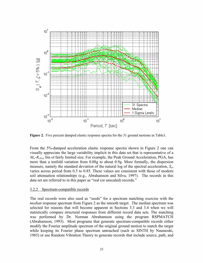
Figure 2. Five percent damped elastic response spectra for the 31 ground motions in Table1. From the 5%-damped acceleration elastic response spectra shown in Figure 2 one can visually appreciate the large variability implicit in this data set that is representative of a Mw-Rclose bin of fairly limited size. For example, the Peak Ground Acceleration, PGA, has more than a tenfold variation from 0.08g to about 0.9g. More formally, the dispersion measure, namely the standard deviation of the natural log of the spectral acceleration, Sa, varies across period from 0.5 to 0.85. These values are consistent with those of modern soil attenuation relationships (e.g., Abrahamson and Silva, 1997). The records in this data set are referred to in this paper as “real (or unscaled) records.” 3.2.2 Spectrum-compatible records The real records were also used as “seeds” for a spectrum matching exercise with the median response spectrum from Figure 2 as the smooth target. The median spectrum was selected for reasons that will become apparent in Sections 3.3 and 3.4 when we will statistically compare structural responses from different record data sets. The matching was performed by Dr. Norman Abrahamson using the program RSPMATCH (Abrahamson, 1993). Most programs that generate spectrum-compatible records either modify the Fourier amplitude spectrum of the original ground motion to match the target while keeping its Fourier phase spectrum untouched (such as SINTH by Naumoski, 1985) or use Random Vibration Theory to generate records that include source, path, and

24

site effects (e.g., RASCAL by Silva and Lee, 1987; and SMSIM by Boore, 2002). All these programs work in the frequency domain. RSPMATCH, however, uses an alternative approach to spectral matching that adjusts the original record in the time domain by adding wavelets to it according to the method developed by Lilhanand and Tseng (1988). The resulting spectrum-compatible records have the elastic response spectra shown in Figure 3. The departure from the target above four seconds is due to the lack of imposed constraints in the matching procedure above that period. Recall that the selected high-pass corner frequency threshold of 0.2Hz suggests using caution when investigating structural responses above a period of 1/(1.25*0.2Hz)=4.0s (according to documentation in http://peer.berkeley.edu/smcat/process.html). Only noise may in fact be present in some of the input signals beyond 4.0s. Similarly, the smallest low-pass corner frequency among all of the records is 20Hz, implying that the structural responses below a period of 0.0625s should be considered with caution as well. In this study we will refer to this set of records as “spectrum-compatible records”.

Figure 3. Five percent damped elastic response spectra for the 31 ground motions matched to the median spectrum in Figure 2.

25

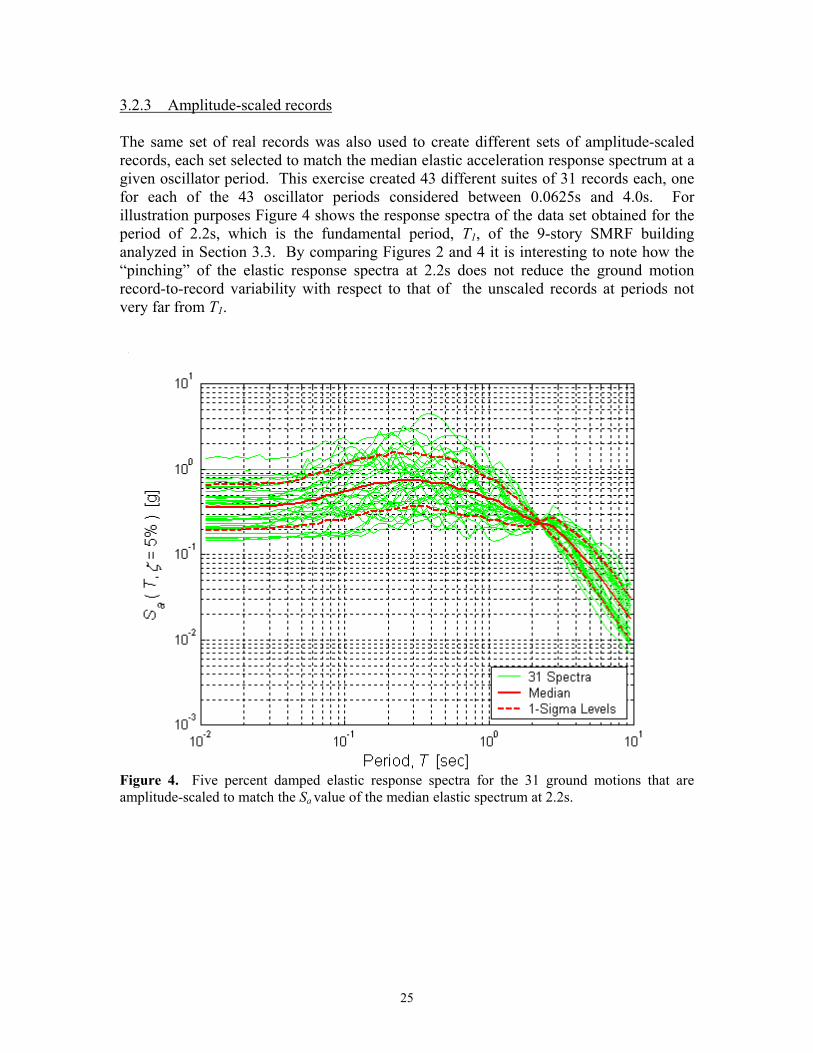
3.2.3 Amplitude-scaled records The same set of real records was also used to create different sets of amplitude-scaled records, each set selected to match the median elastic acceleration response spectrum at a given oscillator period. This exercise created 43 different suites of 31 records each, one for each of the 43 oscillator periods considered between 0.0625s and 4.0s. For illustration purposes Figure 4 shows the response spectra of the data set obtained for the period of 2.2s, which is the fundamental period, T1, of the 9-story SMRF building analyzed in Section 3.3. By comparing Figures 2 and 4 it is interesting to note how the “pinching” of the elastic response spectra at 2.2s does not reduce the ground motion record-to-record variability with respect to that of the unscaled records at periods not very far from T1.

Figure 4. Five percent damped elastic response spectra for the 31 ground motions that are amplitude-scaled to match the Sa value of the median elastic spectrum at 2.2s.

26

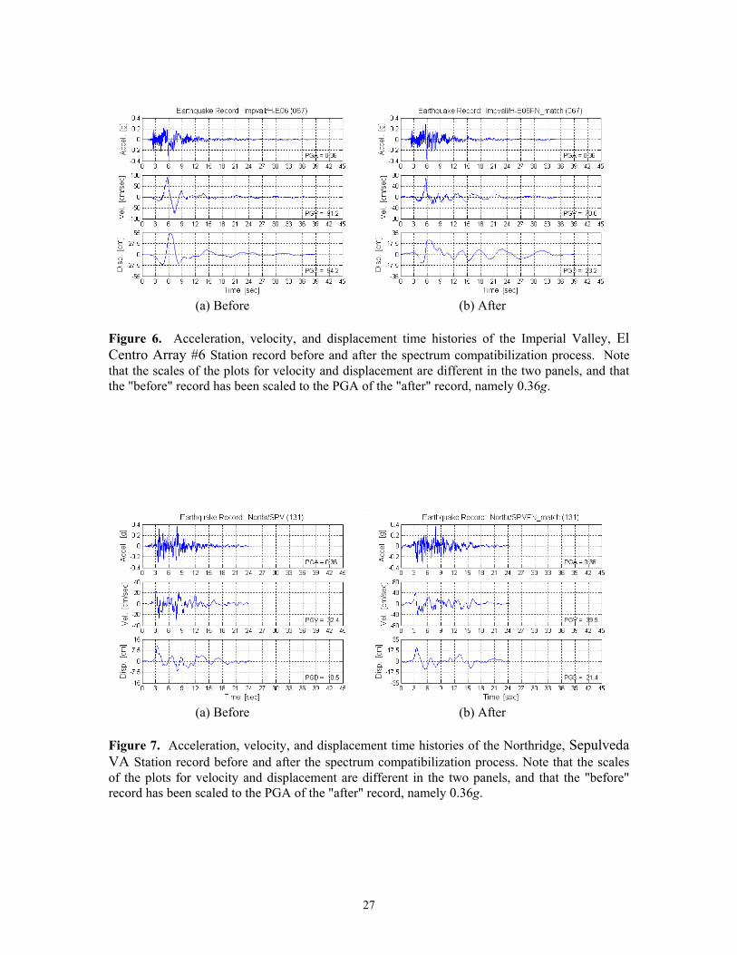
3.2.4 Effects of spectrum matching on recorded ground motion time histories The effects of spectrum matching via the wavelet technique on the time traces of these near-source records are quite complex, and the details differ from case to case. However, from a qualitative point of view two systematic patterns can be detected in the changes introduced to time histories whose frequency contents at long periods (say, above 2s) are either above or below the target median spectrum of the suite. For illustration purposes, the response spectra of two such records, the Imperial Valley, El Centro Array #6 Station record and the Northridge, Sepulveda VA Station record (IMPVALL/H-E06 and NORTHR/SPV, the 7th and 23rd records in Table 1, respectively), are shown in Figure 5, along with the target median spectrum. The time traces of the acceleration, velocity, and displacement of these two records before and after the compatibilization are shown in panels (a) and (b) of Figure 6 and 7, respectively. The comments that follow can be generalized to other records that are not shown here.

Figure 5. Five percent damped elastic response spectra for the IMPVALL/H-E06 (above target at longer periods) and NORTHR/SPV (below target at longer periods) records, before spectrum matching.

27

(a) Before (b) After

Figure 6. Acceleration, velocity, and displacement time histories of the Imperial Valley, El Centro Array #6 Station record before and after the spectrum compatibilization process. Note that the scales of the plots for velocity and displacement are different in the two panels, and that the "before" record has been scaled to the PGA of the "after" record, namely 0.36g.

(a) Before (b) After

Figure 7. Acceleration, velocity, and displacement time histories of the Northridge, Sepulveda VA Station record before and after the spectrum compatibilization process. Note that the scales of the plots for velocity and displacement are different in the two panels, and that the "before" record has been scaled to the PGA of the "after" record, namely 0.36g.

28

Before analyzing the modifications in the signal introduced by the matching process, it should be emphasized that the original records in these two cases tend to be different. The records that are above the median at long periods, on average, have a distinct two-lobe velocity pulse (e.g., panel (a) in Figure 6) whereas those below the median do not show a clear, long-period velocity pulse at all (e.g., panel (a) in Figure 7). In the former case, to lower the spectrum at longer periods the matching process tends either to remove one of the two velocity pulse lobes or to decrease its amplitude. If the process of lowering the spectrum has also brought the high-frequency part of it below the target, then high frequencies are added back into the signal. Both effects are discernible in Figure 6. When the matching process is instead applied to records whose frequency content at long periods needs to be increased, the effects are reversed. The desired amplitude levels at long periods are reached by amplifying the entire spectrum, but no long-period pulses are artificially added to the original time history if no pulses were originally there. If this intermediate adjusting process causes the high-frequency part of the spectrum to overshoot the target, then high frequencies are removed from the signal such that it becomes less “jagged”. Figure 7 shows clearly both effects. To quantitatively summarize the changes introduced in the signals by the matching process, we monitored the average and the dispersion (i.e., the standard deviation of the log) values of three characteristics of the velocity pulse in both the unscaled and the spectrum-matched datasets. More specifically, we considered the number of half-pulses, npulses/2, the pulse period, Tp, and the peak velocity, Vpeak. For example, for the record in Figure 6a (before scaling it to PGA=0.36g) the values of Vpeak, npulses/2, and Tp are equal to 112 cm/s, 2, and 3.7 sec, respectively, whereas for the record in Figure 6b they are equal to 70 cm/s, 1, and 2.4 sec, respectively. Note that there is little ambiguity in how to compute the values of Vpeak and, perhaps, of npulses/2 (we visually “counted” them) but there is no general consensus on how to compute Tp. In this study we estimated Tp by looking at the zero-crossings of the velocity time history pulse that brackets Vpeak. The matching process has the following effects on the three pulse parameters:

• The average value of npulses/2 is reduced by about 20% (from 1.7 to 1.4) while its dispersion remains virtually unchanged (0.41 versus 0.45).

• On average, the value of Tp is increased by about 27% (from 2.2s to 2.8s) and its dispersion is approximately halved (from 0.6 to 0.29)

• The Vpeak is, on average, reduced by 12% (from 60 to 53 cm/s) and its dispersion becomes less than a third (from 0.67 to 0.20).

In summary, as expected the matching process reduces the record-to-record variability of pulse characteristics such as Tp and Vpeak, but, somewhat less expectedly, it increases the period of the pulses and decreases the number of half-pulses.

29

3.3 Response of the SAC 9-story SMRF Building 3.3.1 Description of the computer models

The building analyzed in this section is the 9-story SMRF designed for Los Angeles conditions as part of Phase II of the SAC Steel Project (FEMA 355C, 2000). We will call this building LA9 for short. Figures 8 and 9 show a typical floor plan and one of the perimeter MRF’s, respectively. Only the perimeter frames are moment resisting whereas the interior ones are designed to support gravity loads only. The building was designed according to pre-Northridge specifications, but here we assume that the beam-column connections are ductile. For our analyses we used a model that includes both a perimeter MRF and a consolidated version of the interior gravity frames. This model also assigns some stiffness and strength to the shear connections rather than considering them as “pins.” More details regarding this model can be found in Appendix B of Luco (2002). The SAC LA9 building is strong enough that its response to the real, unscaled records considered here is, on average, at the onset of the post-elastic regime. In order to study how the results change for increasingly larger post-elastic responses, we investigated the seismic performance not only of the as-designed SAC LA9 building described above but also of three additional weaker versions of it. These three weaker variants, which we will call LA91/2, LA91/4, and LA91/8, have the same fundamental period of vibration of LA9 (i.e., 2.2s), but have global lateral yield strengths equal to 1/2, 1/4, and 1/8 of the original one (i.e., strength reduction factors of 2, 4, and 8). The LA91/2, LA91/4, and LA91/8 buildings can be thought as realistic structures designed for progressively less seismic environments in Southern California. As a technicality, note that the three weaker designs were not obtained by the time-consuming process of re-sizing each beam and column. We instead consider the same LA9 building but scale up each one of the 31 records by a factor of two, four, and eight, respectively, and then divide the resulting responses by the same factors. These responses are presumably very similar to those that we would have obtained by subjecting a re-designed weaker structure to the unscaled records. (The results would be identical if the structure were a nonlinear SDOF system.) Let us emphasize that this scaling process should be seen only as a convenient way to investigate the responses of weaker structures subject to the same near-source records of the Mw-Rclose scenario considered here. The intent here is not to investigate the response of the LA9 building to more intense ground motions that may be appropriate for larger magnitude events. Preliminary findings (Somerville, 2003), in fact, suggest that the characteristics of near-source records, such as the period of the velocity pulse, are magnitude-dependent. An amplitude-scaling operation, which does not alter the pulse period, may create near-source records that arguably may not be representative of more intense magnitudes.

30

1 30’−0" 2 30’−0" 3 30’−0" 4 30’−0" 5 30’−0" 6

A

30’−

0"

B

30’−

0"

C

30’−

0"

D

30’−

0"

E

30’−

0"

F

↑N

Figure 8. Typical floor plan of the SAC 9-story building (excerpted from Luco, 2002)

=

=

=

=

W14

x233

W14

x257

W14

x283

W14

x370

W14

x370

=

=

=

=

W14

x257

W14

x283

W14

x370

W14

x455

W14

x500

=

=

=

=

W14

x257

W14

x283

W14

x370

W14

x455

W14

x500

=

=

=

=

W14

x257

W14

x283

W14

x370

W14

x455

W14

x500

=

=

=

=

W14

x257

W14

x283

W14

x370

W14

x455

W14

x500

=

=

=

=

W14

x233

(wea

k−ax

is)

W14

x257

(wea

k−ax

is)

W14

x283

(wea

k−ax

is)

W14

x370

(wea

k−ax

is)

W14

x370

(wea

k−ax

is)

W24x68 W24x68 W24x68 W24x68 W24x68

W27x84 W27x84 W27x84 W27x84 W27x84

W30x99 W30x99 W30x99 W30x99 W30x99

W36x135 W36x135 W36x135 W36x135 W36x135

W36x135 W36x135 W36x135 W36x135 W36x135

W36x135 W36x135 W36x135 W36x135 W36x135

W36x135 W36x135 W36x135 W36x135 W36x135

W36x160 W36x160 W36x160 W36x160 W36x160

W36x160 W36x160 W36x160 W36x160 W36x160

W36x160 W36x160 W36x160 W36x160 W36x160

A30’−0"

B30’−0"

C30’−0"

D30’−0"

E30’−0"

F

Roof

13’−

0"

9th Floor

13’−

0"

8th Floor

13’−

0"

7th Floor13

’−0"

6th Floor

13’−

0"

5th Floor

13’−

0"

4th Floor

13’−

0"

3rd Floor

13’−

0"

2nd Floor

18’−

0"

1st Floor

12’−

0"

P−1

Typ. Splice

6’

Figure 9. Perimeter moment-resisting frame (N-S elevation) of the SAC 9-story building (excerpted from Luco, 2002)

31

3.3.2 Analyses results All of the nonlinear dynamic analyses performed on the LA9 SMRF building and on its three weaker “sisters”, LA91/2, LA91/4, and LA91/8 (i.e., a total of 31 records x 3 sets of records = 93 runs per model) were done using DRAIN-2DX (Prakash et al., 1993). The analyses considered the P-∆ effect. The results obtained for the real records are summarized in Table 2. We gauged the response across the height of the building by the maximum interstory drift ratio, θmax, a parameter that is closely related to its collapse potential. In Table 2 we report the values of θmax for all the records and relevant statistics such as the median value and a measure of the record-to-record variability. The latter measure, which we will call the coefficient of variation (COV) of θmax, is rigorously speaking the standard deviation of the natural logarithm of θmax. Under the assumption that θmax is lognormally distributed, the reported quantity is for all practical purposes numerically identical to the COV(θmax) for values below 0.3. For values exceeding 0.3, the reported quantity gets increasingly smaller than COV(θmax) as the values get larger (for details see page 267 of Benjamin and Cornell, 1970). The record-to-record response variability can also be qualitatively appreciated by looking at the minimum and maximum values of θmax across the 31 records. For example, for the LA9 model θmax ranges from 0.003 to 0.048. Besides drift results, Table 2 shows also the number of analyses that terminated prematurely because equilibrium could not be reached. Here we equate this numerical instability to building “collapse.” Note that the statistics reported in italics at the bottom of Table 2 for the LA91/8 case are “counted” statistics, because the “collapse” cases prevent the calculation of the median and the COV described above. For example, the median value of θmax of 0.028 is the 16th smallest drift value out of the 19 analyses that successfully completed. The reported value of the COV(θmax) is estimated from the counted statistics of the 16th and 50th (i.e., the median) 84th percentiles. The counted statistics for the LA9, LA91/2, and LA91/4 cases are typically within 20% of those reported in Table 2. For the LA91/4 case, the counted statistics are not reported because the single collapse is simply ignored.

32

EarthquakeRecord ID LA9 LA91/2 LA91/4 LA91/8

Impvall/H-BRA 0.011 0.014 0.014 0.012Impvall/H-ECC 0.013 0.016 0.026 "collapse"Impvall/H-EMO 0.032 0.043 0.062 "collapse"Impvall/H-E01 0.003 0.003 0.003 0.004Impvall/H-E04 0.026 0.037 0.065 "collapse"Impvall/H-E05 0.028 0.043 0.077 "collapse"Impvall/H-E06 0.039 0.055 0.033 "collapse"Impvall/H-E07 0.025 0.034 0.052 "collapse"Impvall/H-E08 0.014 0.015 0.017 0.015Impvall/H-E10 0.014 0.015 0.021 0.062Impvall/H-E11 0.010 0.012 0.012 0.008Impvall/H-EDA 0.015 0.022 0.026 0.023Impvall/H-WSM 0.008 0.007 0.011 0.012Superst/B-ICC 0.020 0.015 0.016 0.014

Superst/B-WSM 0.008 0.008 0.009 0.005Northr/LOS 0.019 0.016 0.013 0.015Northr/JEN 0.031 0.026 0.022 "collapse"Northr/NWH 0.031 0.029 0.046 "collapse"Northr/RRS 0.033 0.038 0.062 "collapse"Northr/SPV 0.023 0.019 0.017 0.033Northr/RO3 0.017 0.011 0.008 0.010Northr/SCS 0.035 0.044 "collapse" "collapse"Northr/SCE 0.027 0.028 0.054 "collapse"Northr/SYL 0.030 0.025 0.034 "collapse"

Impvall/H-PTS 0.006 0.006 0.006 0.009Superst/B-PTS 0.045 0.033 0.026 0.024Lomap/WVC 0.023 0.016 0.022 0.066Northr/ARL 0.010 0.010 0.007 0.009Northr/WPI 0.048 0.053 0.040 0.028Northr/PAC 0.012 0.013 0.009 0.011Northr/PKC 0.022 0.015 0.011 0.018

Min 0.003 0.003 0.003 0.004Median 0.018 0.019 0.020 0.028

Max 0.048 0.055 0.077 "collapse"COV 0.64 0.69 0.81 1.15

% collapses 0/31 0/31 1/31 12/31

Max Story Drift Ratio, θ max

Table 2. Nonlinear dynamic drift results for the SAC LA9 building and its three weaker sister buildings obtained using the real record dataset. The LA91/2, LA91/4, and LA91/8 buildings have approximately 1/2, 1/4, and 1/8 of the lateral strength of LA9. See Table 1 for details on the records. The numbers in italics for LA91/8 are counted statistics.

33

Type ofEarthquake Records

UnscaledS a 1 Scaled

Spectrum Compatibilized

Type ofEarthquake Records

Unscaled 0.018 (1.00) 0.019 (1.00) 0.020 (1.00) 0.028 (1.00)S a 1 Scaled 0.018 (0.99) 0.018 (0.95) 0.021 (1.05) 0.034 (1.21)

Spectrum Compatibilized 0.016 (0.89) 0.016 (0.84) 0.017 (0.85) 0.019 (0.68)

Type ofEarthquake Records

Unscaled 0.64 (41) 0.69 (48) 0.81 (65) 1.15 (132)S a 1 Scaled 0.25 (6) 0.22 (5) 0.37 (14) 0.90 (81)

Spectrum Compatibilized 0.09 (1) 0.19 (4) 0.26 (7) 0.54 (29)

3/3111/3112/31LA91/8LA9

0/310/31

Fraction of "Collapses"LA91/4

1/310/31

LA91/4

0/310/31

LA91/2

0/310/31

LA91/8

0/31

LA9 LA91/2 LA91/4

COV (and Min. # Records) of θ max

LA91/8

Median (and Bias) of θ max

LA9 LA91/2

Table 3. Comparison of θmax response statistics for the LA9, LA91/2, LA91/4, and LA91/8 buildings. Sa1 is the 5%-damped spectral acceleration ath the building fundamental period of 2.2s. As in Table 2, the results for LA91/8 (in italics) are “counted statistics” due to the significant number of collapses. Results similar to those shown in Table 2 were also obtained by applying the spectrum-matched records and the amplitude-scaled records to all four versions of the 9-story building. The amplitude-scaled records were obtained by scaling each record to match the Sa value at the fundamental period of vibration of the LA9 building, namely 2.2s (see Figure 4 for their resulting elastic response spectra). In the interest of space, those results are not reported here in their entirety. However, Table 3 presents a comparison of the summary statistics derived from the results of the analyses of the four building models obtained with all three of the record data sets. Multiple comments flow from the examination of the results in Table 3. The first consideration is that the set of spectrum-compatible records seems to generate structural responses that, on average, are systematically lower than those from real records. This is first apparent from the numbers of collapse cases for the LA91/8 model that go from 12 for the real records to 3 for the spectrum-matched ones, a fourfold reduction. The systematic bias in the median θmax ranges from 11% to 32% (i.e., 1.00 minus 0.89 to 0.68) for the four models considered here. It should be noted, however, that due to the limited sample size and the relatively large record-to-record response variability for the

34

unscaled data set, these differences between the median responses from the two suites of records are not statistically significant at any customary level. A two-sided Wilcoxon signed-rank hypothesis test for paired samples shows that the null hypothesis (i.e., the two medians being equal) can be rejected at a significance level of about 9% for LA91/4 and even higher for the other three models. Despite this lack of rigorous statistical significance, the fact that the median response estimates for the spectrum-matched records are consistently lower than those for the real records for all four buildings is, however, a compelling indication than this bias is indeed real. The observed bias generated by spectrum-matched records is in substantial agreement with that reported by Carballo and Cornell (2000). They note that the negative bias may be due to the asymmetric effect that peaks and valleys that are present in the elastic spectrum of real records have on nonlinear structural response. A peak in the period range above T1 larger than the ordinates of the average spectrum for that Mw-Rclose scenario makes a record more damaging than average. Similarly, a valley in the period range above T1 with opposite characteristics makes a record less damaging than average. The former effect, however, is more pronounced than the latter. Therefore, the spectrum-matching exercise that removes both peaks and valleys from the smooth target elastic spectrum, in general, artificially renders a record more benign than those in nature. On the other hand, the amplitude-scaled records do not seem to introduce any statistically significant bias in the responses, even for the LA91/8 model (again, due to the limited sample size and relatively large record-to-record variability). We will see in the next section, however, that this observation does not necessarily hold for structures of shorter fundamental periods. Besides the analysis of potential bias, the second important aspect is the reduced response variability to the “manipulated” records. The drastic decline of two to seven times in the spectrum-matched record-to-record response variability shown in Table 3 makes such records more “efficient” than real ones for response estimation purposes. In plain words, the same accuracy in estimating the “true” median structural response can be achieved with many less spectrum-matched records than real ones. To a lesser degree a similar comment is valid for amplitude-scaled records, whose reduction in response variability, however, is generally less significant. The quantification of the record “efficiency” issue is provided by the number in parentheses in the middle panel of Table 3. These are the minimum numbers of records necessary to achieve ±10% accuracy in the estimate of the median response given the amount of response variability reported next to it. For example, for the LA91/2 case four spectrum-matched records (or five amplitude-scaled ones) will provide the same accuracy of 48 real records in estimating the median θmax. Of course, if one were to use spectrum-compatible records, the median response obtained with the four records should be corrected for the systematic bias that such records seem to introduce. For example, assuming that the bias estimates computed here with a limited sample size are accurate, the median response of 0.016 for the LA91/2 case should be multiplied by 1/0.86. Similar comments hold for amplitude-scaled records. The results in Table 3, however, do not

35

warrant an adjustment to the median computed response for this building should amplitude-scaled records be used instead.

3.4 Response of Elastic-Perfectly-Plastic SDOF Systems

3.4.1 Description of the SDOF systems As mentioned earlier, we analyzed 43 elastic-perfectly-plastic SDOF systems with period, T1, ranging from 0.0625 to 4.0s, and for each T1 we considered four different yield strengths, Fy, Fy

R=2, FyR=4, and Fy

R=8. For any given value of T1, the strength, Fy, is the force that corresponds to the yield spectral displacement dy, where dy is the median 5%-damped spectral displacement at T1 for the set of 31 real records. The values of Fy

R=2, Fy

R=4, and FyR=8 are obtained by dividing Fy by two, four, and eight, respectively. The

symbol R in the superscript refers to the strength reduction factor commonly used in codes. By design, the responses to the 31 real records of the 43 oscillators with yield strengths equal to the values of Fy at each period T1 are, on average, at the onset of nonlinearity. At the other extreme, the responses of the weaker SDOF systems with Fy

R=8

yielding strength are, on average, severely in the nonlinear range. The set-up of this SDOF-system experiment mimics that of the 9-story building in the previous section. It is intended to give a breadth to the results in terms of range of both structural period and severity of post-elastic responses and also to provide an opportunity for checking the consistency of the results of nonlinear MDOF and SDOF structures with the same elastic fundamental period.

3.4.2 Analyses results This section presents a distillation of the results of about 16,000 nonlinear dynamic analyses performed on the 43 elastic-perfectly-plastic SDOF systems with four yield strengths levels (Fy, Fy

R=2, FyR=4, and Fy

R=8) subject to the three ground motion datasets of 31 records each.

36

Figure 10. Median inelastic displacement response spectra for the four sets of SDOF systems with strengths equal to Fy, Fy

R=2, FyR=4, and Fy

R=8 subject to the three suites of 31 unscaled, amplitude-scaled, and spectrum-matched ground motions. The dashed line is at 2.2s, the fundamental period of the LA9 building. The displacement response spectra for the unscaled, amplitude-scaled, and spectrum-compatible ground motions are displayed in log-log scale in Figure 10. The spectra are presented for all four SDOF system strength levels, one spectrum for each of the three ground motion data sets. We can assume here that the median displacement response spectrum for the unscaled records is an unbiased estimate of the true median spectrum for this Mw-Rclose earthquake scenario. As expected given the design of this experiment, the three spectra for the nearly elastic case (i.e., Fy yield strength) are, for all practical purposes, indistinguishable. Hence, no bias is introduced in the elastic (or mildly inelastic) responses by the use of amplitude-scaled or spectrum-matched records. Figure 10 shows, however, that the median inelastic response spectra (namely those for the Fy

R=2, FyR=4, and Fy

R=8 yield strengths) for the amplitude-scaled and the spectrum-compatible data sets do not coincide with the unbiased target, particularly at shorter periods. The median spectrum from the amplitude-scaled records tends to be above the target, while the opposite is true for the median spectrum from the compatibilized records. Within the limitation of the sample size used in this study, this discrepancy implies that the use of either amplitude-scaled or

37

spectrum-compatible records introduces a certain degree of bias of opposite sign in the computed structural response. The bias appears to be positive for amplitude-scaled records, which means that the scaling process has made them, on average, more damaging than unscaled records for the same scenario event. On the contrary, spectrum-matched records appear to be, as for the SAC 9-story building, less damaging than their real, unscaled counterparts (i.e., the bias tends to be negative). Before analyzing these results in more detail it is worth noting again that the limitations in sample size and the relatively large response variability mean that the bias of opposite sign introduced by using spectrum-matched and amplitude-scaled records are not statistically significant at any customary significance level (e.g., 5% or 10%). The consistency of this bias for all strength levels and all oscillator periods, however, is compelling despite the lack of formal statistical support. The comments that follow are to be interpreted in this light. The quantification of the bias is clearer in Figure 11, which shows the ratio of the median spectra from the amplitude-scaled and the spectrum-matched records to the median spectrum from the unscaled records. The amount of bias across periods is given by the departure from unity. From this figure it is clear that the bias is both period- and yield-strength-dependent. The bias introduced by amplitude-scaled records for not very severe nonlinear responses (Fy

R=2 and FyR=4 cases) oscillates in the period range considered (i.e., 0.0625-4.0s)

between approximately 0 and +25%. The bias tends to stabilize for highly nonlinear responses (i.e., the Fy

R=8 case) to about +10% across the entire period range. On the other hand, the bias introduced by spectrum-matched records for moderately nonlinear responses tends to be of the opposite sign and to oscillate from approximately 0 to more than –30% for periods below 0.16s. For severely nonlinear responses, again, the bias becomes approximately constant across period with a value of about –10%. We have already reported an intuitive explanation for the negative bias introduced by spectrum-matched records. The qualitative argument that supports the positive bias resulting from amplitude-scaled ones is conceptually similar. Records belonging to the same Mw-Rclose scenario that need a significant boost to reach the target Sa value are, on average, in a valley at the period, T1, involved in the scaling process. This means that when scaled up to the target Sa value, such records will show a peak in the period range longer than T1 that is swept by the structure when entering the post-elastic response regime. In contrast, records that need to be severely down-scaled to the target Sa value at T1, on average, tend to be on or near a peak of their jagged spectrum. Therefore, after the down-scaling the spectrum will have a valley rather than a peak in the periods greater than T1. As stated earlier, the increment in severity of structural responses introduced by peaks is comparatively larger than the response reduction due to valleys (Carballo and Cornell, 2000). This qualitative argument explains, at least partially, the positive bias in the median response of amplitude-scaled records.

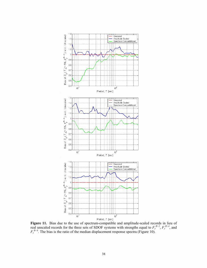
38

Figure 11. Bias due to the use of spectrum-compatible and amplitude-scaled records in lieu of real unscaled records for the three sets of SDOF systems with strengths equal to Fy

R=2, FyR=4, and

FyR=8. The bias is the ratio of the median displacement response spectra (Figure 10).

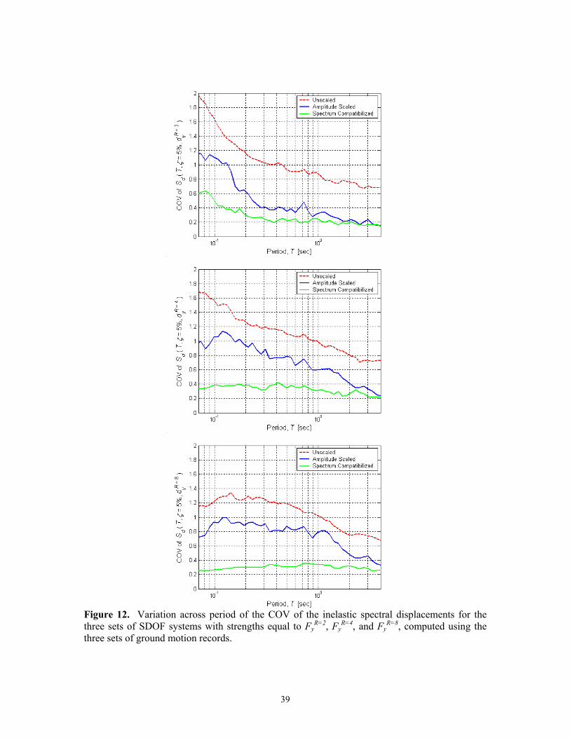
39

Figure 12. Variation across period of the COV of the inelastic spectral displacements for the three sets of SDOF systems with strengths equal to Fy

R=2, FyR=4, and Fy

R=8, computed using the three sets of ground motion records.

40

The analysis of Figure 12 confirms that the use of amplitude-scaled and, especially, of spectrum-matched records makes the record-to-record variability in the structural response drop substantially. From a practical standpoint, again, this translates into a smaller number of analyses needed to reach the same level of accuracy in the estimate of the median response if these records are adopted. This result is particularly useful and somewhat novel for short-period SDOF systems. For stiff SDOF systems the COV of the response for unscaled records is so large as to prevent the estimation of the median response within a reasonable accuracy unless an impractically large number of runs is performed. For example, for a 0.3s SDOF system, about 120 real records would be needed to estimate its median response for this Mw-Rclose scenario within ±10%. Only about 10 spectrum-compatible records would be sufficient to achieve the same level of accuracy. Finally, it is worth noting that the bias and the response dispersion measure for the four versions of the SAC 9-story building (i.e., LA9, LA91/2, LA91/4, and LA91/8) that are reported in Table 3 are generally in good agreement with the SDOF results for the same fundamental period of 2.2s and strength levels (i.e., Fy, Fy

R=2, FyR=4, and Fy

R=8) in Figures 11 and 12. The only exception may be the lack of bias in the 2.2s SDOF system results for the Fy and Fy

R=2 cases that contrasts with a –11% to –32% bias in Table 3. We should keep in mind, however, that these relatively small differences cannot be statistically detected with this sample size. As a final point, we did not make any provision for the elastic-perfectly-plastic SDOF systems to fail at a given spectral displacement. Therefore, a comparison with the number of collapse cases observed for the LA91/4, and LA91/8 buildings could not be made.

3.5 Summary and Conclusions

In this study we compared and contrasted the use of real, unscaled records versus spectrum-matched and amplitude-scaled ones for the estimation of inelastic response of nonlinear SDOF and MDOF structures of different strengths and vibration periods. We considered a suite of 31 near-source, forward-directivity ground motion records from intermediate magnitude events that were rotated orthogonal to the fault strike. On the structural side, we used the SAC 9-story SMRF building designed for Los Angeles conditions and three sister buildings with reduced lateral strengths. To give breadth to our results we also considered elastic-perfectly-plastic SDOF systems with four different strength levels and vibration periods between 0.0625s and 4.0s. The response of all these structures subject to these different sets of ground motions were evaluated via time-domain step-by-step integration of the equations of motion. The focus of this study is prompted by an interest in real applications. Because of a lack of “appropriate” real records, engineers in fact often resort to using time histories that are either matched to a smooth target spectrum or scaled to be “consistent” with a target ground-motion level. The effects that spectrum matching and scaling have on the nonlinear response estimates are, however, not well understood. Here we statistically compared the responses of three sets of “consistent” ground motions representative of the

41

same magnitude-distance (Mw-Rclose) scenario. One comprises the 31 real records mentioned above, while the other two were derived from it by spectrum-matching and amplitude-scaling those records to the median elastic spectrum of the batch. The most important findings of this study can be summarized as follows:

• The use of spectrum-matched records drastically reduces the response variability (by 60% to 80%), which in turn translates into needing many less such records to estimate the median response for the same level of accuracy. This result is significant especially for short-period structures whose large record-to-record response variability practically precludes the use of real accelerograms for response prediction (more than 100 records are needed for achieving ±10% accuracy in the median response). The median response to spectrum-compatible records, however, appears to be slightly more benign (up to about 30% in some short-period cases) than that caused by real, unscaled ground motions.

• The use of amplitude-scaled ground motions also reduces the record-to-record response variability, but to a lesser degree (from 20% to 75%). Hence, scaled records that keep their jagged response spectrum are less “efficient” for response estimation purposes than records that have been compatibilized to a smooth target spectrum. Amplitude-scaled records also seem to introduce a bias in the response but of opposite sign (up to approximately 25% in some cases). The scaling process appears to make records slightly more damaging than those in nature.

• Both the bias and variability reduction introduced by using spectrum-matched and amplitude-scaled records vary with severity of nonlinear response and with period of the structure.

• The limited sample size used in this study and the large record-to-record response variability prevents us from concluding that the observed response bias is statistically significant at any customary significance level (e.g., 5% or 10%). Current research by the authors with more, but not exclusively, near-source earthquake records will help in this respect.

• The time-domain, wavelet-based spectrum-matching process used here tends to slightly decrease the number of velocity half-pulses, to increase the velocity pulse period, and to reduce its peak.

The results presented in this paper are strictly valid for the near-source records and the MDOF and SDOF structures considered here. They may not necessarily apply to other more ordinary records from a different Mw-Rclose scenario, and/or to other structures with different characteristics than those considered here. Also, the authors do not necessarily imply that the observations made here on the use of spectrum-matched records are applicable to other spectrum-compatibilization techniques. A study on the generality and applicability of these findings to other cases is left to future research.

42

3.6 Acknowledgements We are very grateful to Norm Abrahamson and Brian Chiou for the fruitful discussions that led to the seeding idea for this study. We also thank Walt Silva for providing us with the original records, and Nick Gregor and Norm Abrahamson for spectrum matching them. The work greatly benefited from the comments that we received at the PEER Lifelines quarterly meetings, especially from Cliff Roblee and Tom Shantz. Comments received by Allin Cornell, Helmut Krawinkler, Greg Deierlein, and Eduardo Miranda, to whom we presented preliminary results of this study, are also very much appreciated. This research was made possible by the grant from the PEER Lifelines Program, Research Subagreement No. SA3592.

3.7 References Abrahamson. N.A. (1993). Non-Stationary Spectral Matching Program RSPMATCH”, User Manual, July 16. Abrahamson, N.A., and Silva, W.J. (1997). ``Empirical Response Spectra Attenuation Relations for Shallow Crustal Earthquakes'', Seism. Res. Lett., Vol. 68, No.1, pp. 94-127. Benjamin, J.R., and C.A. Cornell (1970). Probability, Statistics, and Decision for Civil Engineers, McGraw Hill Book Company, New York, NY. Boore, D.M. (2002). Fortran Programs for Simulating Ground Motions for Earthquakes: Version 2.0 – A revision of OFR 96-80-A“, Revision of U.S. Geological Survey Open File Report OFR 00-509, August 8, http://www.geol.vt.edu/iasphand/85_Software/8513boore/smsim_manual.pdf Carballo, J.E., and C.A. Cornell (2000). “Probabilistic Seismic Demand Analysis: Spectrum Matching and Design”, Report No. RMS-41, Department of Civil and Environmental Engineering, Reliability of Marine Structures Program, Stanford University, Stanford, CA, July. Federal Emergency Management Agency (FEMA) (2000). ``State of the Art Report on System Performance of Steel Moment Frames Subject to Ground Shaking”, FEMA 355C, September 2000. Federal Emergency Management Agency (FEMA) (2001). ``NEHRP Recommended Provisions for Seismic Regulations for New Buildings and Other Structures'', 2000 Edition, Part 1 - Provisions, FEMA 368, March 2001. Lilhanand, K., and W.S. Tseng (1988). “Development and Application of Realistic Earthquake Time Histories Compatible with Multiple Damping Response Spectra”,

43

Proceedings of 9th World Conference on Earthquake Engineering, Tokyo, Japan, Vol II, pp. 819-824. Luco, N. (2002). “Probabilistic Seismic Demand Analysis: SMRF Connection Fractures, and Near-Source Effects”, Ph.D. Dissertation, Department of Civil and Environmental Engineering, Stanford University, Stanford, CA, June. Luco, N., and P. Bazzurro (2003). “Beyond Spectral Quantities to Improve Structural Response Estimation”, submitted to Earthquake Engineering and Structural Dynamics, September. Naumoski, N. (1985). “SYNTH Program – Generation of Artificial Acceleration Time History Compatible with a Target Spectrum”, McMaster Earthquake Engineering Software Library, Dept. of Civil Engineering and Engineering Mechanics, McMaster University, Hamilton, Canada. Prakash, V., Powell, G.H., and S. Campbell (1993). “DRAIN-2DX Base Program Description ad User Guide, Version 1.10”, Report No. UCB/SEMM-93/17, Dept. of Civil Engineering, University of California at Berkeley, Berkeley, CA. Silva, W.J., and K. Lee (1987). “WES RASCAL Code for Synthesizing Earthquake Ground Motions”, Report 24, Miscellaneous Paper S-73-1, Prepared for Department of the Army, US Army Corps of Engineers, Washington, DC. Somerville, P.G., Simth, N.F., Graves, R.W., and N.A. Abrahamson (1997). “Modification of Empirical Strong Ground Motion Attenuation Relations to Include the Amplitude and Duration Effects of Rupture Directivity”, Seismological Research Letters, Vol. 68, No. 1, January/February. Somerville, P.G. (2003). “Magnitude Scaling of the Near Fault Rupture Directivity Pulse”, Physics of the Earth and Planetary Interiors, Vol. 137, pp. 201-212.

44

4 Beyond Spectral Quantities to Improve Structural Response

Estimation Abstract: The objective of this study is to investigate whether the use of “non-stationary” features of ground motion time histories in addition to more conventional ground motion intensity measures (e.g., spectral values) significantly improves the accuracy in the prediction of structural response. The response of structures is computed here via nonlinear dynamic analysis. The 9-story SAC steel moment-resisting frame (SMRF) designed for Los Angeles and three additional weaker variants are used as test cases. We have subjected these four sister buildings to a suite of 31 near-source, forward-directivity, strike-orthogonal ground motion records from four intermediate-magnitude earthquakes. Prior to the analyses, these records were compatibilized to the median elastic spectrum of the suite to simplify the statistical search for characteristics of the signal beyond the spectral values that can serve as additional response predictors. The results of this study show that ground motion records, per-se, are neither damaging nor benign. The damageability of a record can only be measured in relation to a particular structural vibration period and specific strength. Hence, using record characteristics that do not account for the period and the strength of the structure are not likely to be “good” predictors of its response. For the structures considered here, characteristics of the velocity pulse, such as the number of half-pulses, npulses/2, the pulse period, Tp, and the peak velocity, Vpeak, and the duration of the record do not appreciably improve the accuracy of the response estimates beyond that achieved by the use of spectral values alone. The inelastic displacement of an elastic-perfectly-plastic SDOF system with similar period and strength of the MDOF structure and, more innovatively, the first “significant” peak displacement of the elastic SDOF oscillator with the same fundamental period of the MDOF structure appear to be more promising candidate predictors. The use of the latter deserves more attention in future research. 4.1 Introduction For structural engineers in seismic regions, the relationship between earthquake ground motion and structural response is of primary concern. Modern nonlinear dynamic analysis software allows engineers to more realistically estimate the structural response and damage resulting from a time history of earthquake ground motion (i.e., an accelerogram). Although an accelerogram is typically the only characteristic of ground motion that is directly measured, in many cases it is more convenient to quantify the ground motion data by means of one or more scalar parameters derived from the accelerogram, such as peak ground acceleration (PGA) or elastic spectral quantities for acceleration, velocity, or displacement (Sa, Sv, and Sd, respectively). Ground motion parameters such as these are critical, for example, in estimating (or "predicting") the likelihood of specified levels of seismic response, of structural and non-structural damage, and ultimately of monetary loss for a given structure at a specific site or for a portfolio of structures at many sites. In order to perform any of these risk assessment tasks efficiently and precisely, one or more ground motion parameters that are strongly correlated with structural response are necessary. In the past decades many researchers have historically linked the damage effectiveness of an earthquake time history to intensity measures such as PGA or, more recently, elastic

45

spectral quantities. PGA is now widely regarded as a relatively poor indicator of structural damage (Sewell, 1989, Bazzurro and Cornell, 1994). Spectral quantities, instead, have been observed to be efficient predictors of structural performance for first-mode dominated structures subject to “ordinary” (namely, not pulse-like) ground motions. For multi-mode dominated structures, a combination of elastic spectral accelerations at different oscillator frequencies can be used to achieve adequate predictive power (e.g., Bazzurro and Cornell, 2002). Particularly for pulse-like ground motions, inelastic spectral quantities (e.g., Luco, 2002; Luco and Cornell, 2003) have been demonstrated to be more efficient. In this latter case, however, the development of empirical attenuation relationships for inelastic spectral quantities is especially challenging. AT the time of this writing, research with this aim is ongoing at Stanford University under the supervision of Prof. Allin Cornell. Some researchers have considered time-domain rather than frequency-domain characteristics of the earthquake record. For example, Iwan et al. (1998), MacRae and Roeder (1999), Alavi and Krawinkler (2001), and Cuesta and Ascheim (2001), among many others, have pointed out that that time-domain features of near-source records, such as the amplitude and the period of the velocity pulse, considerably affect building responses to near-source ground motions. Alavi and Krawinkler (2001) and Somerville (2003) have also developed simple predictive equations for pulse period and amplitude. Given the remaining variability in the inelastic structural response for ground motions with the same elastic spectrum (quantified in this paper), engineering intuition suggests that it may be more effective to include parameters of non-stationary time-domain “features” of the input ground motion in a pool of structural response predictors (along with frequency-domain-based quantities). This may be especially true particularly for near-source records. In this study we intend to test this hypothesis. We address the response prediction of a multi-mode-dominated building of four different “strength” levels subject to near-source, forward-directivity, strike-orthogonal ground motion records. 4.2 Earthquake Ground Motion Records The ground motions considered are the same as those summarized in Table 1 of the companion paper (Luco and Bazzurro, 2003). The database consists of 31 near-source (closest source-to-site distance, Rclose, less than 16km), strike-normal ground motion components recorded on stiff soil under forward directivity conditions from four different shallow crustal earthquakes in California. The moment magnitude, Mw, of these events is 6.5 for the Imperial Valley, 1979, Earthquake (14 records), 6.7 for the Superstition Hills, 1987, and the Northridge, 1993, Earthquakes (3 and 13 records, respectively), and 6.9 for the Loma Prieta, 1989, Earthquake (1 record). The 31 5%-damped elastic acceleration response spectra, along with the median and the median plus and minus one standard deviation spectra, are shown in Figure 2 of the same companion paper. The limited range of variation of both Mw and Rclose makes this record data set a good representation of a realistic Mw-Rclose scenario.

46

To facilitate the search of time-domain characteristics of the signal to include in a suite of predictors along with elastic spectral quantities, we used ground motions that have been spectrum-matched to the median elastic spectrum of the data set. The entire set of compatibilized records share, by definition, the same elastic response spectrum. Therefore, the effectiveness of each additional predictor other than spectral quantities is immediately apparent without the need to resort to more complicated multiple regression analysis with both Sa’s and the newly proposed predictors. The intent here is to keep the use of statistics to a bare minimum so as not to confuse the message with unnecessarily complicated technicalities. The spectrum matching was done by Dr. Norman Abrahamson using his time-domain, wavelet-based software RSPMATCH (Abrahamson, 1993). Because of the high-pass corner frequency value of 0.2Hz or lower adopted during the filtering process, and the low-pass corner frequency value of 20Hz, a few of these records may contain only noise outside the range of about 0.0625s to 4s (http://peer.berkeley.edu/smcat/process.html). With this in mind, the spectrum matching was focused on this period range. More details about the time histories before and after the compatibilization process are reported in the companion paper. We emphasize again, however, that in this article we only deal with the spectrum-matched records. The non-stationary time-domain features that we consider as potential response predictors are the number of half-pulses, npulses/2, the pulse period, Tp, and the peak velocity, Vpeak. In addition, we also considered the duration of the record, TH, computed as the difference in times corresponding to 95% and 5% of the total Arias intensity (Trifunac and Brady, 1975). Note that despite being derived from near-source, strike-normal components, not all the records show a distinct velocity pulse, and those that do may have an odd or even number of lobes. (This applies to the original, un-modified records as well.) The records that do not show a clear pulse tend to have short Tp values and are assigned a value of npulses/2 equal to one. The average number of npulses/2 in this data set is 1.4. The parameter Vpeak varies from about 20 cm/s to over 70 cm/s with a median value of 53 cm/s, while Tp ranges approximately from 1s to 5s, with a median value of 2.8s. The energy-based duration TH also varies considerably from record to record, from about 6s to 24s. In an effort to address the ambiguity that is involved in the computation of Vpeak and, especially, of Tp, we estimated their values in two different ways. The first and most straightforward approach is simply based on reading the maximum value of Vpeak from the original velocity time history and estimating Tp by looking at the zero-crossings of the velocity pulse that bracket the peak value. The second and more complicated approach applies the same concepts mentioned above to a velocity time history derived from the original one by a signal processing technique known as the Empirical Mode Decomposition (EMD) (e.g., Huang et al., 1998; Loh et al., 2001). The EMD approach decomposes the original signal, through a procedure called “sifting”, into a number of non-stationary nearly-orthogonal components (or “modes”). The sum of all the modes recovers the original signal, within a small tolerance. Such decomposition preserves the nonlinear and non-stationary characteristics of the complete signal while identifying

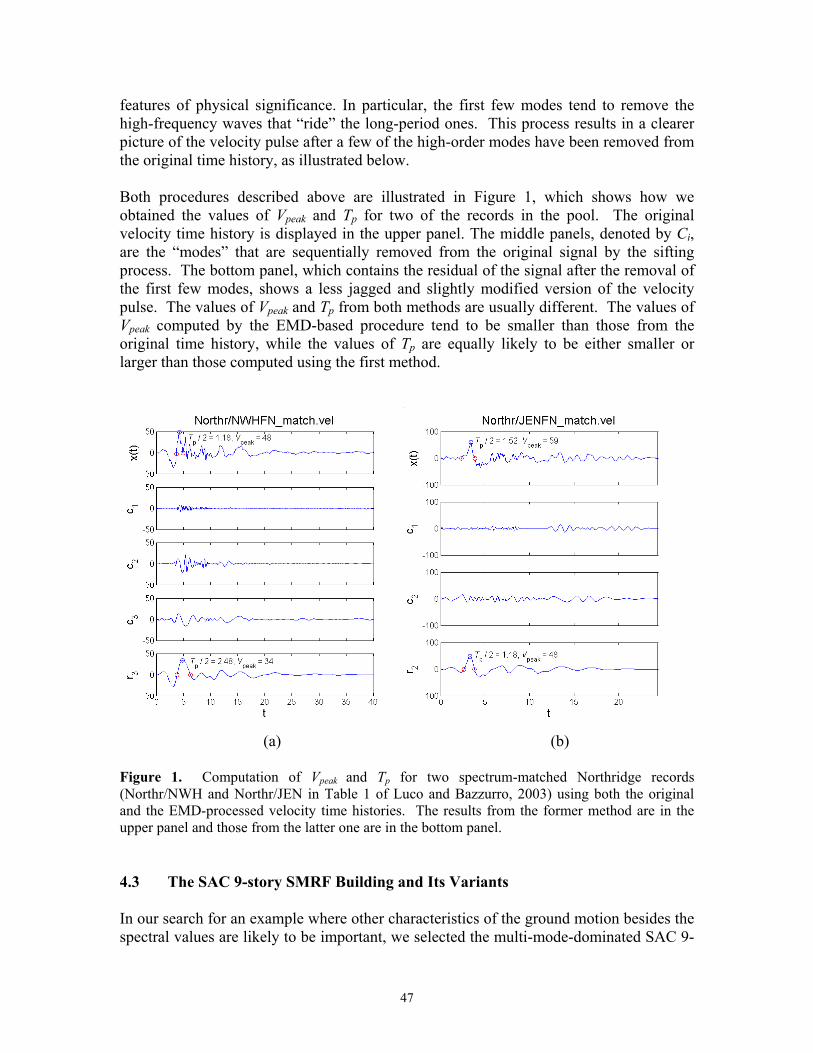
47

features of physical significance. In particular, the first few modes tend to remove the high-frequency waves that “ride” the long-period ones. This process results in a clearer picture of the velocity pulse after a few of the high-order modes have been removed from the original time history, as illustrated below. Both procedures described above are illustrated in Figure 1, which shows how we obtained the values of Vpeak and Tp for two of the records in the pool. The original velocity time history is displayed in the upper panel. The middle panels, denoted by Ci, are the “modes” that are sequentially removed from the original signal by the sifting process. The bottom panel, which contains the residual of the signal after the removal of the first few modes, shows a less jagged and slightly modified version of the velocity pulse. The values of Vpeak and Tp from both methods are usually different. The values of Vpeak computed by the EMD-based procedure tend to be smaller than those from the original time history, while the values of Tp are equally likely to be either smaller or larger than those computed using the first method.

(a) (b) Figure 1. Computation of Vpeak and Tp for two spectrum-matched Northridge records (Northr/NWH and Northr/JEN in Table 1 of Luco and Bazzurro, 2003) using both the original and the EMD-processed velocity time histories. The results from the former method are in the upper panel and those from the latter one are in the bottom panel. 4.3 The SAC 9-story SMRF Building and Its Variants In our search for an example where other characteristics of the ground motion besides the spectral values are likely to be important, we selected the multi-mode-dominated SAC 9-

48

story Steel Moment-Resisting Frame (SMRF) building designed for Los Angeles conditions. We will call it here the LA9 building. As in the companion paper, to explore the realm of more severe nonlinear responses, we also considered three weaker sister buildings, the LA91/2, LA91/4, and LA91/8, which have, respectively, about 50%, 25%, and 12.5% of the lateral strength of LA9 (i.e., strength reduction factor, R, equal to 2, 4, and 8, respectively). All four buildings have a fundamental period of vibration equal to about 2.2s. As explained in Luco and Bazzurro (2003), the weaker versions of the LA9 building are obtained not by re-designing weaker structures but by scaling up all the 31 records by two, four, and eight times and dividing the resulting responses by the same factors. respectively. This alternative is quite convenient as it presumably provides similar (identical for SDOF structures) results to those that could be obtained by re-designing the LA9 building and keeping the records unscaled. The LA91/2, LA91/4, and LA91/8 variants can be thought of as realistic structures designed for progressively less seismic environments in Southern California. More details on the LA9 model can be found in the companion paper and in Luco (2002). Note that although LA9 was designed according to pre-Northridge practices, here the beam-column connections are modeled as ductile. 4.4 Is an Accelerogram Damaging or Benign for all Structures of the Same Period? It is widely known that a ground motion record may have a higher than average content at some periods and be more deficient than average at others. Hence, basic engineering principles suggest that a record may be highly damaging for some structures and less severe for others of different periods. This is the reason why a ground motion parameter that accounts for the fundamental period, T1, of a structure (e.g., Sa at T1) is a more powerful response predictor than one that does not (e.g., PGA). What is less obvious is the extent to which a record that is either very damaging or very benign for a structure of a given fundamental period of vibration maintains its effectiveness in creating damage to all structures of the same period. In other words, are there any non-stationary features of a signal that particularly affect the response of all structures at a given period? The preceding question is very pertinent to the main goal of this study. If the answer is affirmative, and if such features of a signal can be predicted in terms of the basic random variables Mw and Rclose used in Probabilistic Seismic Hazard Analysis (PSHA), then the parameters of these features can be used as response predictors in the same fashion as PGA or Sa are used today. This would require only building new attenuation relationships, a conceptually straightforward task. If the answer is negative, and a record's damaging ability depends not only on the period of a structure but also, say, on its “strength,” then one could conclude that there is nothing intrinsic in a ground motion time history that makes it particularly damaging or benign for all structures with the same fundamental period. If this second option is true, for a ground motion parameter to be an effective response predictor it should account for the strength of the structure as well. To test the effectiveness of a ground motion record in causing larger or smaller than average responses of structures with the same vibration period but different strengths, we run the 31 spectrum-matched records through the LA9, LA91/2, LA91/4, and LA91/8 building models. We gauged the response by the largest peak value over time of inter-

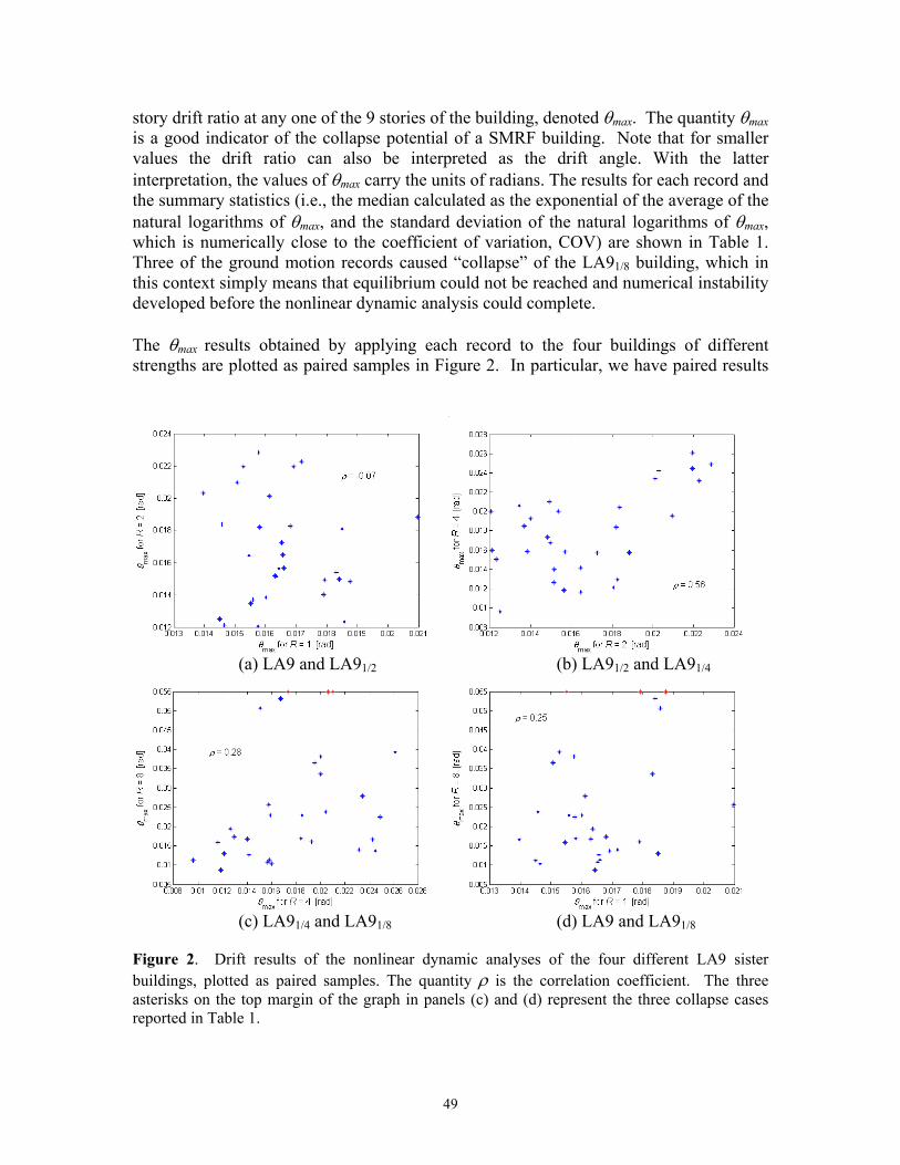
49

story drift ratio at any one of the 9 stories of the building, denoted θmax. The quantity θmax is a good indicator of the collapse potential of a SMRF building. Note that for smaller values the drift ratio can also be interpreted as the drift angle. With the latter interpretation, the values of θmax carry the units of radians. The results for each record and the summary statistics (i.e., the median calculated as the exponential of the average of the natural logarithms of θmax, and the standard deviation of the natural logarithms of θmax, which is numerically close to the coefficient of variation, COV) are shown in Table 1. Three of the ground motion records caused “collapse” of the LA91/8 building, which in this context simply means that equilibrium could not be reached and numerical instability developed before the nonlinear dynamic analysis could complete. The θmax results obtained by applying each record to the four buildings of different strengths are plotted as paired samples in Figure 2. In particular, we have paired results

(a) LA9 and LA91/2 (b) LA91/2 and LA91/4

(c) LA91/4 and LA91/8 (d) LA9 and LA91/8 Figure 2. Drift results of the nonlinear dynamic analyses of the four different LA9 sister buildings, plotted as paired samples. The quantity ρ is the correlation coefficient. The three asterisks on the top margin of the graph in panels (c) and (d) represent the three collapse cases reported in Table 1.

50

EarthquakeRecord ID LA9 LA91/2 LA91/4 LA91/8

Impvall/H-BRA 0.019 0.012 0.015 0.051Impvall/H-ECC 0.015 0.021 0.020 0.037Impvall/H-EMO 0.018 0.015 0.020 0.034Impvall/H-E01 0.018 0.018 0.012 0.013Impvall/H-E04 0.017 0.018 0.013 0.017Impvall/H-E05 0.017 0.022 0.023 0.014Impvall/H-E06 0.019 0.015 0.017 "collapse"Impvall/H-E07 0.016 0.018 0.018 0.017Impvall/H-E08 0.016 0.014 0.018 0.023Impvall/H-E10 0.014 0.020 0.024 0.017Impvall/H-E11 0.021 0.019 0.016 0.026Impvall/H-EDA 0.016 0.015 0.014 0.017Impvall/H-WSM 0.016 0.013 0.021 "collapse"Superst/B-ICC 0.016 0.015 0.013 0.019

Superst/B-WSM 0.016 0.012 0.020 0.038Northr/LOS 0.015 0.016 0.012 0.016Northr/JEN 0.017 0.016 0.014 0.013

Northr/NWH 0.016 0.020 0.023 0.028Northr/RRS 0.015 0.018 0.020 0.024Northr/SPV 0.016 0.016 0.012 0.009Northr/RO3 0.015 0.012 0.016 0.010Northr/SCS 0.015 0.022 0.026 0.039Northr/SCE 0.016 0.014 0.016 0.023Northr/SYL 0.015 0.013 0.010 0.011

Impvall/H-PTS 0.016 0.023 0.025 0.022Superst/B-PTS 0.017 0.017 0.016 0.011Lomap/WVC 0.018 0.015 0.021 "collapse"Northr/ARL 0.018 0.015 0.017 0.053Northr/WPI 0.017 0.022 0.024 0.014Northr/PAC 0.018 0.014 0.019 0.016Northr/PKC 0.017 0.016 0.016 0.011

Min 0.014 0.012 0.010 0.009Median 0.016 0.016 0.017 0.019

Max 0.021 0.023 0.026 "collapse"COV 0.09 0.19 0.26 0.54

% collapses 0/31 0/31 0/31 3/31

Max Story Drift Ratio, θ max

Table 1. Nonlinear dynamic drift results for the SAC LA9 building and its three weaker sister buildings. The LA91/2, LA91/4, and LA91/8 buildings have approximately 1/2, 1/4, and 1/8 the lateral strength of LA9.

51

that are almost linear (for LA9) to those that are severely nonlinear (for LA91/8), and other combinations in between. It is visually apparent that the trend, when it exists, is positive but extremely mild. More rigorously, the correlation coefficient, ρ, ranges from -0.07 in the LA9 vs. LA91/2 comparison, to 0.56 in the LA91/2 vs. LA91/4 case. In plain words, this mild correlation implies that a record that causes a larger than average response in a “strong” building (e.g., LA9) of vibration period T1 (here 2.2s) may very well be more benign than average for a weaker building with the same fundamental period (e.g., LA91/4). This statement is even more interesting if we remember that these results are generated by records that share the same elastic response spectrum (that is, by records that cause the same maximum elastic response in SDOF systems at all periods) and by structures that, aside for the yield strength, are identical. Hence, records appear to be damaging or benign only in relation to a structure with a particular period of vibration and strength. No time-domain feature, at least for this record set and these structures, seems to make an accelerogram either extremely severe or extremely "gentle," per-se, for all structures with the same vibration period. As suggested earlier, an immediate consequence of this finding is that an effective response predictor to be considered along with the spectral values should account for the strength of the structure, not just its fundamental period of vibration. To gain insights into the reasons for this somewhat unexpected lack of strong correlation, we repeated the same nonlinear dynamic analyses for a simpler but related structure, namely an elastic-perfectly-plastic SDOF oscillator with the same vibration period, T1, of 2.2s as the four SAC 9-story sister buildings, and with Fy estimated from a static pushover curve for LA9 (Luco, 2002). As in Luco and Bazzurro (2003), we considered four different yield strength levels, Fy, Fy

R=2, FyR=4, and Fy

R=8. The values of FyR=2, Fy

R=4, and Fy

R=8 are obtained by dividing Fy by two, four, and eight, respectively. The letter R in the notation (not to be confused with the distance, Rclose) refers to the widely used strength reduction factor. The corresponding values of yield displacements in the four cases are dy=30cm, dy

R=2=15cm, dyR=4=7.5cm, and dy

R=8=3.75cm. The paired results for the SDOF systems shown in Figure 3 confirm that, in the SDOF case, the lack of strong correlation already observed for the four 9-story sister buildings also holds. To study this phenomenon in more detail, we singled out two records, Northr/SCS (#137) and Impvall/H-E06 (#067) (see Figure 4 for their seismograms). Record #137 creates severe post-elastic responses consistently at all the three yield strength levels Fy

R=2, FyR=4, and Fy

R=8, while record #067 is fairly severe at the FyR=2 and

FyR=8

levels, but rather benign at the FyR=4 level. Recall that because the two records

have been spectrum-matched, their peak elastic responses (i.e., Fy strength level) are equal.

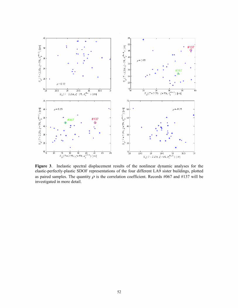
52

#137

#067

#137

#067

#137#067 #137#067

Figure 3. Inelastic spectral displacement results of the nonlinear dynamic analyses for the elastic-perfectly-plastic SDOF representations of the four different LA9 sister buildings, plotted as paired samples. The quantity ρ is the correlation coefficient. Records #067 and #137 will be investigated in more detail.

53

Figure 4. Displacement, velocity, and displacement time histories of the two spectrum-matched records Northr/SCS (#137) and Impvall/H-E06 (#067).

54

Figure 5 shows the time traces of the SDOF displacement created by the record #137 for all four levels of yield strength. The horizontal dotted-dashed lines mark the yield displacements in the four cases, while the open circles represent the maximum displacement over time, namely Sd

i. The black line, which refers to the elastic response obtained for the Fy case, has its maximum absolute value equal to dy = 30cm, as expected, and oscillates around the zero-displacement line. The other three responses all enter the post-elastic regime before the record is over. Loosely speaking, if the ground motion is strong enough the displacement tends to deviate and sometimes to progressively drift away from the zero line. All four time traces coincide until the yield displacement corresponding to each of the Fy

R=2, FyR=4, and Fy

R=8 cases is exceeded, and after that time the traces depart from one another. In general, the amount of separation seems to be somewhat dependent on how far beyond the yield displacement the first significant peak is. Figure 5 shows that, in the three nonlinear time histories for the Fy

R=2, FyR=4, and Fy

R=8

cases, the first peak that considerably exceeds the yield levels of dyR=2, dy

R=4, and dyR=8,

respectively, is negative and occurs at about 4 seconds. Note that the displacement for the Fy

R=8 yield strength case already exceeded dyR=8=3.75cm before 3s, but not to an

extent large enough to cause a major departure from linearity. In the response prediction section below we will address the meaning of “significant exceedance” beyond the yield displacement in a quantitative manner. The excursion to the post-elastic regime in all three Fy

R=2, FyR=4, and Fy

R=8 cases is so severe than the displacement cannot recover and it keeps oscillating around large negative values. This record is damaging for all the yield strengths.

Figure 5. Time histories of the SDOF displacements generated by Record #137 for yield displacements dy=30cm, dy

R=2=15cm, dyR=4=7.5cm, and dy

R=8=3.75cm. The open circles represent the maximum values over time, which are plotted in Figure 3.

55

Figure 6. Time histories of the SDOF displacements generated by Record #067 for yield displacements dy=30cm, dy/2=15cm, dy/4=7.5cm, and dy/8=3.75cm. The open circles represent the maximum values over time, which are plotted in Figure 3. A different picture can be seen in Figure 6, which shows the displacement time traces generated by record #067. In this case, the first large excursion is again negative and occurs around 6 seconds. The exceedance of the yield displacement is so significant for the Fy

R=8 case that, again, the system drifts away to large negative displacements. For the Fy

R=4 case however, the exceedance of the yield displacement is not severe enough to prevent the system from being pushed back by the next large peak of ground motion in the opposite direction. After being re-centered, the displacement keeps oscillating around relatively small values. In the third and last Fy

R=2 case, the first exceedance of the yield displacement is minor, but the next ground motion peak pushes the SDOF system well beyond yield in the positive direction. In summary, this record is very “benign” at the Fy

R=4 level and fairly severe at the Fy

R=2 and FyR=8 levels.

This qualitative rationale as to why the maximum inelastic displacement can be either small or large is generally applicable to other ground motions in the suite. The analysis of these displacement time histories yields important ancillary insight into the response prediction problem. The hope is that the first significant peak of the elastic response, P1

e, which is an easy-to-compute parameter that implicitly carries the notion of both vibration period, T1, and yield displacement, dy, could be used, along with Sa, as a predictor of the response of a MDOF structure characterized by T1 and dy. The hope is strengthened by the particular nature of the near-source ground motion records that tend to exhibit only one or two pulses that cause the largest part of the response to be concentrated in a very limited number of large cycles. Although not tested here, we expect the knowledge of

56

P1e to be somewhat less helpful in estimating the maximum inelastic response to

“ordinary” ground motions that present many more peaks in time. There is a clear advantage in using a parameter of a linear elastic SDOF system response, such as P1

e, instead of a parameter of a nonlinear SDOF system response, such the inelastic peak response, Sd

i, itself. To develop new attenuation laws for the latter parameters, seismologists would need to start computing the time histories of inelastic SDOF oscillators with different strength levels, which is currently not done. Seismologists, however, routinely calculate the entire displacement time history of elastic SDOF systems, but only to retain their maximum values (i.e., the elastic spectral values). Extracting the value of P1

e for different levels of dy would be trivial and could be achieved with the same tools in use today. Following this lead, in the following section we will investigate the use of P1

e as a predictor of the inelastic Sd

i of SDOF systems of different strengths but the same period. More importantly, we will also test this predictor in estimating the maximum inter-story drift ratio of the four 9-story SMRF buildings. 4.4 Non-Stationary Features of a Ground Motion Record as Response Predictors 4.4.1 Characteristics of the velocity pulse and ground motion duration Figures 7, 8, and 9 show scatter plots of θmax, the response parameter adopted to measure the response of the LA9, LA91/2, LA91/4, and LA91/8 buildings, versus the velocity-pulse characteristics of pulse period, Tp, peak velocity, Vpeak, and number of half-pulses, npulses/2. Each asterisk represents the nonlinear dynamic analysis result for one of the 31 records in the set. (Recall that all the records are spectrum-matched). Again, the three asterisks in the upper margin of the graphs for the LA91/8 building represent the collapse cases listed in Table 1. The values of Tp and Vpeak reported in this section are those found using the EMD-based approach presented earlier. All the conclusions made here, however, remain valid when the other sets of Tp and Vpeak values from the original time-histories are used instead. A visual inspection of Figure 7 shows a mild positive trend only for the LA91/4 building, which implies that longer pulse periods, on average, generate larger responses in this case. This is to be expected, to the extent that the post-elastic events that occur during the ground shaking tend to elongate the effective structural vibration period to values close to the larger Tp’s in this data set. Miranda and his co-workers (as reported in ATC, 2002) and Alavi (2001) have found similar results. As we will see later, though, this correlation is too weak to be helpful in response prediction. Furthermore, for the LA9, LA91/2, and LA91/8 buildings there is almost no correlation between Tp and θmax. Given that Tp does not reflect the strength level, it is not too surprising that the correlation of Tp with θmax is non-negligible for only one of the strength levels (i.e., R=4)

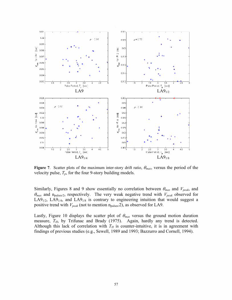
57

LA9 LA91/2

LA91/4 LA91/8 Figure 7. Scatter plots of the maximum inter-story drift ratio, θmax, versus the period of the velocity pulse, Tp, for the four 9-story building models. Similarly, Figures 8 and 9 show essentially no correlation between θmax and Vpeak, and θmax and npulses/2, respectively. The very weak negative trend with Vpeak observed for LA91/2, LA91/4, and LA91/8 is contrary to engineering intuition that would suggest a positive trend with Vpeak (not to mention npulses/2), as observed for LA9. Lastly, Figure 10 displays the scatter plot of θmax versus the ground motion duration measure, TH, by Trifunac and Brady (1975). Again, hardly any trend is detected. Although this lack of correlation with TH is counter-intuitive, it is in agreement with findings of previous studies (e.g., Sewell, 1989 and 1993; Bazzurro and Cornell, 1994).

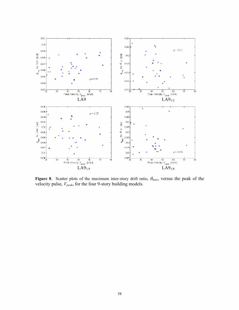
58

LA9 LA91/2

LA91/4 LA91/8 Figure 8. Scatter plots of the maximum inter-story drift ratio, θmax, versus the peak of the velocity pulse, Vpeak, for the four 9-story building models.

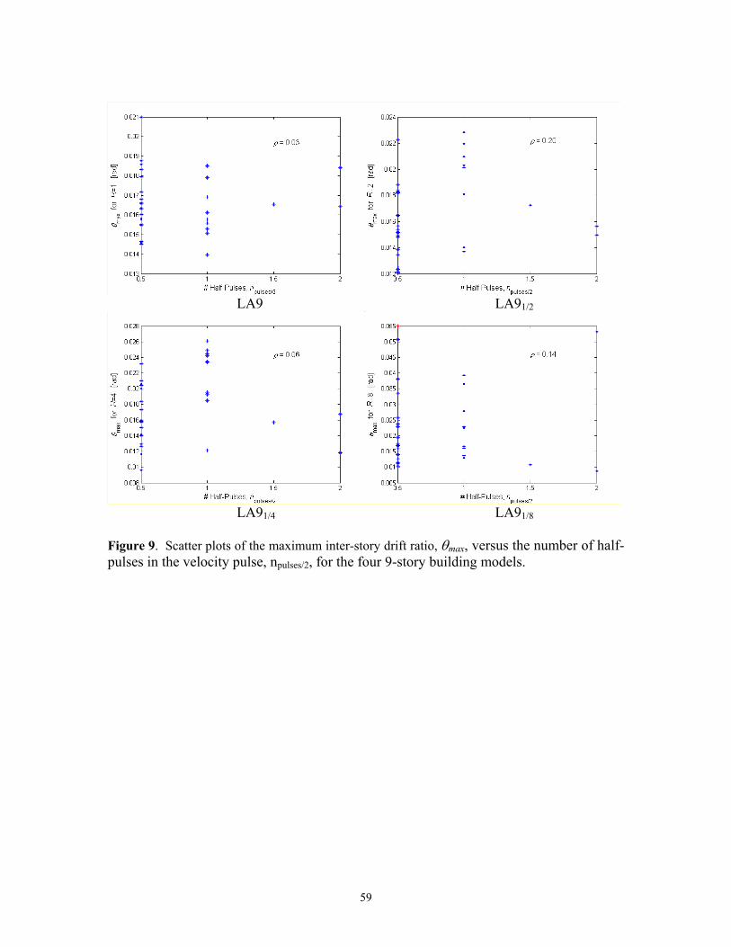
59

LA9 LA91/2

LA91/4 LA91/8 Figure 9. Scatter plots of the maximum inter-story drift ratio, θmax, versus the number of half-pulses in the velocity pulse, npulses/2, for the four 9-story building models.

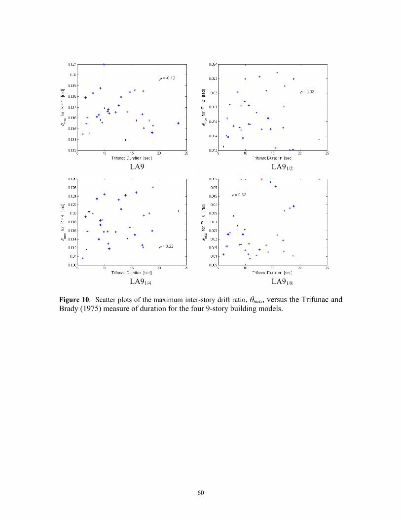
60

LA9 LA91/2

LA91/4 LA91/8 Figure 10. Scatter plots of the maximum inter-story drift ratio, θmax, versus the Trifunac and Brady (1975) measure of duration for the four 9-story building models.

61

More formally, we also performed linear regression analyses of θmax on the four candidate predictors Tp, Vpeak, npulses/2, and TH, considered both separately and in different combinations. We are interested in monitoring the reduction in record-to-record response variability “explained” by including any predictor (or combinations of predictors) in the regression model. The quantitative results are shown in Table 2, where the first row represents the initial benchmark, namely the variability explained by the response spectrum alone. Clearly the extra variability explained by the other predictors is negligible. This means that the characteristics of the velocity pulse, Tp, Vpeak, npulses/2, and the duration of the record, TH, alone or in the combination considered do not add any useful information for the prediction of θmax that is not already carried by the spectral values. In other words, if the spectral values are already used for the prediction of θmax, and here they implicitly are via spectrum-matching, then the knowledge of Tp, Vpeak, npulses/2, and TH does not seem to improve the prediction. Note that this conclusion is not in contrast with the findings by Iwan et al. (1998), MacRae and Roeder (1999), Alavi and Krawinkler (2001), and Cuesta and Ascheim (2001). These researchers used real records with different response spectra. If spectral values are not used as predictors, then the information carried by the pulse characteristics becomes valuable for response estimation purposes.

None (Spect. Comp.)

Trifunac Duration

T p & V peak (via EMD)

Predictor(s)

0.09 0.19 0.26

COV of θ max

LA91/8

0.49

0.26

0.24

0.49

0.51

LA9

0.09

0.09 0.19

0.19

LA91/2 LA91/4

Table 2. Measure of the record-to-record variability of θmax for the SAC LA9, LA91/2, LA91/4, and LA91/8 buildings that is left “unexplained” by a linear regression that includes the predictor(s) in the first column. The results for LA91/8 exclude the three earthquake records in Table 1 that caused collapse. 4.4.2 Inelastic spectral displacement and first significant elastic peak displacement Figure 11 shows the maximum inter-story drift ratio, θmax, for the three inelastic 9-story SMRF sister buildings (i.e., LA91/2, LA91/4, and LA91/8) plotted versus the inelastic spectral displacement, Sd

i, of the nonlinear SDOF oscillator with corresponding T1 and dy. The results for LA9 are not included because the unexplained response variability is already so small (i.e., COV=0.09) that its reduction would not have any practical inpact on response prediction. The correlation, which ranges from 0.66 for LA91/2 to 0.78 for LA91/8, is, in general, higher than that obtained for any of the combinations of Tp, Vpeak, npulses/2, and TH considered. Interestingly, the corresponding scatter plots of θmax versus P1

e displayed in Figure 12 show that the levels of correlation of P1e and Sd

i with θmax are

62

comparable for LA91/2 and LA91/4; for LA91/8, however, the correlation with P1e is only

half as strong. These optimized correlations for P1e are achieved by considering as the

“significant” peak the first one that exceeds 1.2 x dyR=2 for LA91/2, 1.8 x dy

R=4 for LA91/4, and 2.0 x dy

R=8 for LA91/8. Recall from Figures 5 and 6 that the elastic response had to exceed the yield displacement of the nonlinear structures by a considerable margin for the inelastic response to drift away to large values. The multipliers used here maximize the correlation between P1

e and Sdi. A limited study on nonlinear SDOF systems

discussed below suggests, however, that such values are fairly stable for other structures with the same levels of nonlinear response but different initial vibration periods.

LA91/2

LA91/4 LA91/8 Figure 11. Scatter plots of the maximum interstory drift ratio, θmax, of the three inelastic 9-story sister buildings versus the inelastic displacement of a SDOF system with the corresponding fundamental period of vibration (2.2s) and yield displacement.

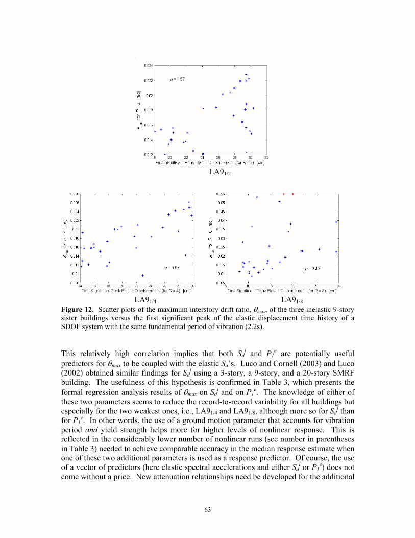
63

LA91/2

LA91/4 LA91/8 Figure 12. Scatter plots of the maximum interstory drift ratio, θmax, of the three inelastic 9-story sister buildings versus the first significant peak of the elastic displacement time history of a SDOF system with the same fundamental period of vibration (2.2s). This relatively high correlation implies that both Sd

i and P1e are potentially useful

predictors for θmax to be coupled with the elastic Sa’s. Luco and Cornell (2003) and Luco (2002) obtained similar findings for Sd

i using a 3-story, a 9-story, and a 20-story SMRF building. The usefulness of this hypothesis is confirmed in Table 3, which presents the formal regression analysis results of θmax on Sd

i and on P1e. The knowledge of either of

these two parameters seems to reduce the record-to-record variability for all buildings but especially for the two weakest ones, i.e., LA91/4 and LA91/8, although more so for Sd

i than for P1

e. In other words, the use of a ground motion parameter that accounts for vibration period and yield strength helps more for higher levels of nonlinear response. This is reflected in the considerably lower number of nonlinear runs (see number in parentheses in Table 3) needed to achieve comparable accuracy in the median response estimate when one of these two additional parameters is used as a response predictor. Of course, the use of a vector of predictors (here elastic spectral accelerations and either Sd

i or P1e) does not

come without a price. New attenuation relationships need be developed for the additional

64

parameters, the covariance structure between all the parameters involved needs to be studied, and a more complex PSHA approach for a vector of variables rather than for a scalar quantity needs to be used. The first two tasks, however, are only numerically but not conceptually challenging, and the tool for the vector hazard estimation is already available (Bazzurro and Cornell, 2002). As mentioned earlier, the authors are aware of a body of research ongoing at Stanford University under the supervision of Prof. Allin Cornell that aims at developing attenuation relationships for Sd

i.

None (Spect. Comp.) 0.19 (4) 0.26 (7) 0.49 (24)

First (in time) Significant Peak Elastic Displacement 0.16 (3) 0.21 (4) 0.45 (20)

S d (T 1=2.2s, ζ =5%, d y =30cm/R ) 0.15 (2) 0.20 (4) 0.30 (9)

LA91/2 LA91/4Predictor LA91/8

COV of θ max

Table 3. Measure of the record-to-record variability of θmax for the SAC LA91/2, LA91/4, and LA91/8 buildings left “unexplained” by a linear regression model that includes the predictor(s) in the first column. The number in parenthesis represents the minimum number of records needed to estimate the median response with ±10% accuracy. The results for LA91/8 exclude the three earthquake records in Table 1 that caused collapse. To supplement the results on the use of P1

e for response prediction with different vibration periods, we investigated its efficiency in estimating the peak nonlinear response of simpler nonlinear structures other than the 9-story SMRF buildings. This side-study also intended to verify whether the margins of 20%, 80%, and 100% above the yield displacements (i.e., dy

R=2, dyR=4, and dy

R=8, respectively) that were observed to provide high correlation for Sd

i at a period of 2.2s, are stable across period. We considered three sets of elastic-perfectly-plastic SDOF oscillators with fundamental periods of 1.0s, 2.2s (the same as the three variants of the LA9 building), and 4.0s, and three different yield displacements, dy

R=2, dyR=4, and dy

R=8. The value of dy is set equal to the ordinate of the elastic displacement target (or median) spectrum at the corresponding period, and, as before, dy

R=2, dyR=4, and dy

R=8 are obtained by dividing dy by 2, 4, and 8, respectively. A

period of 1.0s can be associated with, say, a 3-story SMRF building, whereas a period of 4.0s can be representative of, say, a 20-story SMRF building. Figure 13 shows the scatter plots of P1

e versus Sdi for oscillators with period of 2.2s and

yield displacements equal to dyR=2, dy

R=4, and dyR=8. Table 4 summarizes the results of

the regression analyses for all three periods considered, in the same format used for Tables 2 and 3. By inspecting Table 4 it is apparent that the correlation between Sd

i and P1

e remains high for different SDOF systems when threshold values of 20%, 80%, and

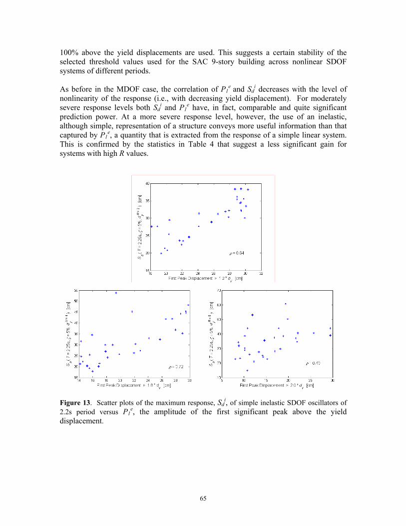
65

100% above the yield displacements are used. This suggests a certain stability of the selected threshold values used for the SAC 9-story building across nonlinear SDOF systems of different periods. As before in the MDOF case, the correlation of P1

e and Sdi decreases with the level of

nonlinearity of the response (i.e., with decreasing yield displacement). For moderately severe response levels both Sd

i and P1e have, in fact, comparable and quite significant

prediction power. At a more severe response level, however, the use of an inelastic, although simple, representation of a structure conveys more useful information than that captured by P1

e, a quantity that is extracted from the response of a simple linear system. This is confirmed by the statistics in Table 4 that suggest a less significant gain for systems with high R values.

Figure 13. Scatter plots of the maximum response, Sd

i, of simple inelastic SDOF oscillators of 2.2s period versus P1

e, the amplitude of the first significant peak above the yield displacement.

66

Table 4. Test of the efficiency of using P1

e as a predictor of the maximum displacement response, Sd

i, of nonlinear oscillators of three vibration periods. The numbers in parentheses indicate the minimum number of records needed to achieve ±10% accuracy in the median response estimate. 4.5 Summary and Conclusions This article presents findings on the use of time-domain ground motion characteristics in addition to the customary elastic spectral values as predictors of nonlinear structural response. We have limited our study to steel moment-resisting frames subject to near-source accelerograms recorded in forward-directivity conditions. To simplify the statistical analyses, the ground-motion records were spectrum-matched to the median elastic spectrum of the suite prior to computing the structural response via nonlinear dynamic analysis. The structural response gauge is the maximum inter-story drift ratio, a quantity that is well correlated with the collapse potential of these types of buildings. We considered the response of the SAC 9-story building designed for Los Angeles conditions and of three weaker variants with the same initial elastic fundamental period but lower “strengths”. To broaden the applicability of our results we also considered simple elastic-perfectly-plastic oscillators with different vibration periods and yield displacements.

Elastic Response Spectrum(Spectrum Compatibles)

+ First (in time) Significant Peak Elastic Displacement

Elastic Response Spectrum(Spectrum Compatibles)

+ First (in time) Significant Peak Elastic Displacement

Elastic Response Spectrum(Spectrum Compatibles)

+ First (in time) Significant Peak Elastic Displacement

(In parantheses): Number of seismograms necessary to estimate median S dI with 10% uncertainty.

0.27

0.18

0.19

0.11

0.14

0.10 0.19

0.23

0.21

0.31

0.25

0.30

0.20 (4)

(7)

(3)

(4)

(1)

(2)

(1)

(7)

0.34

(9)

(8)

(11)

0.26

0.29

0.31

0.27

(5)

(3)

T = 1.0 sec

T = 2.2 sec

T = 4.0 sec

(9)

(6)

(9)

(4) (8)

GivenDispersion of S d

I ( T , ζ =5% , d yR )

R =2 R =4 R =8

67

This study demonstrates that there is nothing intrinsic in the time signal of a ground motion record that makes it either very damaging or very benign to structures of different periods and strengths. There is only a mild correlation between the nonlinear response of a strong and of a weak structure with the same initial fundamental period of vibration caused by the same record. The damage potential of a record is a meaningful concept only when addressed in conjunction with a structure of a given period and strength. With this premise in mind, we showed that the most widely used ground motion time-domain characteristics of near-source records (namely the amplitude and the period of the velocity pulse, and the number of half-pulses in the time history) do not seem to carry additional response-prediction power not already provided by the customary elastic spectral quantities. Similarly, the duration of the record is not a useful additional predictor, at least for assessing the response of ductile building models. These four ground motion parameters, notice, do not explicitly account for period or strength of the structure. As emphasized above, for a ground motion parameter to have significant predictive power, it should account for the period and strength of the structure of interest. In the realm of possible predictors of this nature, we investigated the use of the inelastic spectral displacement of a SDOF oscillator with the same period and strength as the structure of interest, and of the first “significant” peak of the elastic displacement response of a SDOF system of the same period. By significant we mean the first peak that considerably exceeds the yield level of the target structure (see body of paper for quantification). Both parameters, and especially the former, appear to be well correlated with the adopted response measure and provide a significant reduction of the record-to-record response variability from the level achieved by using spectral values alone. This reduction translates into running fewer records to achieve the same level of accuracy in the median response. The first significant peak of the elastic response is a novel predictor introduced in this study that warrants further research. Its predictive power appears to be effective for near-source ground motions that cause moderately intense inelastic responses in very few response cycles. Intuitively, we expect it to be less useful for ordinary far-field ground motions. When effective, such as in some of the cases studied here, its use may prove to be very practical because it will not require seismologists to compute nonlinear responses of SDOF systems, a task that they are not yet accustomed to performing. The linear response of SDOF oscillators is already calculated in estimating the spectral values for attenuation relationships. Only a minimal amount of extra work would be required. 4.6 Acknowledgements We are very grateful to Norm Abrahamson and Brian Chiou for the fruitful discussions that led to the seeding idea for this study. We also thank Walt Silva for providing us with the original records, and Nick Gregor and Norm Abrahamson for spectrum matching them. The work greatly benefited from the comments that we received at the PEER Lifelines quarterly meetings, especially from Cliff Roblee and Tom Shantz. Comments

68

received by Allin Cornell, Helmut Krawinkler, Greg Deierlein, and Eduardo Miranda, to whom we presented preliminary results of this study, are also very much appreciated. This research was made possible by the grant from the PEER Lifelines Program, Research Subagreement No. SA3592. 4.7 References Abrahamson. N.A. (1993). Non-Stationary Spectral Matching Program RSPMATCH”, User Manual, July 16. Alavi, B., and H. Krawinkler (2001). “Effects of Near-Fault Ground Motions on Frame Structures”, Rept. No. 138, The John A. Blume Earthquake Engineering Center, Dept. of Civil and Environmental Engineering, Stanford University, Stanford, CA. Applied Technology Council (ATC) (2002). “A Progress Report on ATC-55: Evaluation and Improvements of Inelastic Seismic Analysis Procedures (Fall 2002)”, by C. Comartin, Redwood City, CA. Bazzurro, P., and C.A. Cornell (1994). “Seismic Hazard Analysis of Nonlinear Structures. I: Methodology”, Journal of Structural Engineering, Vol. 120, No.11, pp. 3320-3344. Bazzurro, P., and C.A. Cornell (2002). “Vector-valued Probabilistic Seismic Hazard Analysis (VPSHA)''. Proceedings of 7th U.S. National Conference on Earthquake Engineering, Boston, MA, July 21-25, Paper No. 61. Cuesta, I., and M.A. Ascheim (2001). “Using Pulse R-factors to Estimate Structural Response to Earthquake Ground Motions”, Report CF/54/01-03, Mid-America Earthquake Center, CD release 01-03, Urbana, Illinois. Iwan, W.D., Huang, C-T., and A.C. Guyader (1998). “Evaluation of the Effects of Near-Source Ground Motions”, Report Developed for the PG&E/PEER Program, California Institute of Technology, Pasadena, CA. Huang, N.E., Shen, Z., Long, S.R., Wu, M.C., Shih, H.H., Zheng, Q., Yen, N-C., Tung, C.C., and H.H. Liu (1998). “The Empirical Mode Decomposition and the Hilbert Spectrum for Nonlinear and Non-Stationary Time Series Analysis”, Proc. Of the Royal Society of London, Vol. 454, pp. 903-995, London, UK. Loh, C-H., Wu, T-C., and N.E. Huang (2001). ”Application of the Empirical Mode Decomposition-Hilbert Spectrum Method to Identify Near-Fault Ground-Motion Characteristics and Structural Responses”, B.S.S.A., Vol. 91, pp. 1339-1357, October.

69

Luco, N. (2002). “Probabilistic Seismic Demand Analysis: SMRF Connection Fractures, and Near-Source Effects”, Ph.D. Dissertation, Department of Civil and Environmental Engineering, Stanford University, Stanford, CA, June. Luco, N., and P. Bazzurro (2003). “Inelastic Structural Responses to Elastic-Spectrum-Matched and to Amplitude-Scaled Earthquake Records”, submitted to Earthquake Engineering and Structural Dynamics, September. Luco, N., and C.A. Cornell (2003). “Structure-Specific Scalar Intensity Measures for Near-Source and Ordinary Earthquake Ground Motions”, Submitted for Publication to Earthquake Spectra. MacRae, G.A., and C.W. Roeder (1999). “Near-Field Ground Motion Effects on Short Structures”, Report Developed for the PG&E/PEER Program, Dept. of Civil Engineering, University of Washington, Seattle, WA. Sewell, R.T. (1989). “Damage Effectiveness of Earthquake Ground Motion: Characterizations Based on the Performance of Structures and Equipment”, Ph.D. Dissertation, Dept. of Civil Engineering, Stanford University, Stanford, CA, January. Sewell, R.T. (1993). “Impacts of Earthquake Strong-Motion Duration on Inelastic Structural Response Factors and on Ground-Motion Damage Potential”, RIE Report prepared for California Strong Motion Instrumentation Program (CSMIP), Sacramento, CA. Somerville, P.G. (2003). “Magnitude Scaling of the Near Fault Rupture Directivity Pulse”, Physics of the Earth and Planetary Interiors, Vol. 137, pp. 201-212. Trifunac, M.D., and A.G. Brady (1975). “A Study of the Duration of Strong Earthquake Ground Motion”, B.S.S.A., Vol. 65, pp. 581-626.

70

5. Conclusions and Recommendations This study originally intended to identify time-domain, non-stationary features of near-source, forward-directivity ground motions that cause large inelastic responses in steel moment-resisting frame structures. The hope was that the existence or absence of such features in ground motions would be informative in predicting their effectiveness in producing large responses and, therefore, structural damage. To investigate this issue we used an advanced signal processing technique, the Empirical Mode Decomposition (EMD) method, which is tailored for nonstationary time histories. To facilitate the search, we applied the EMD to the records mentioned above after they had been “matched” to a target elastic response spectrum. The findings of this study have demonstrated that the objective is attainable only when the ground motion damage effectiveness is associated with a specific structure (e.g., of a given initial elastic fundamental period of vibration and yield strength). In other words, there is nothing intrinsic in a ground motion record that makes it benign or severe for all structures. This conclusion could have been partially expected, but, perhaps, not to the extent shown here. Even the knowledge of the structural period alone is not sufficient to assess the ability of a record to cause a large response; the yield strength is needed as well. In fact, it turns out that there is a very mild correlation between the peak responses to the same record of two structures with the same period but different strengths. A record could easily induce larger than average responses for a “weak” structure and smaller than average responses for a “strong” one. For the SMRF structure and near-source ground motions considered here, the velocity pulses were identified as the non-stationary time domain features that are responsible for damage effectiveness of the ground motions. Of course, this is not an original finding, although it was corroborated here by nonlinear dynamic analyses that used both the entire record and only its pulse as extracted by the EMD technique. More interestingly, however, this study showed that characteristics of the velocity pulse, such as the number of lobes and its peak amplitude and period, are not useful predictors of structural responses if paired with conventional spectral values. The extra information contained in that knowledge of the pulse characteristics is simply not important enough to increase the prediction accuracy. In the realm of non-stationary time-domain features, we identified a novel ground motion parameter that, unlike the characteristics of a velocity pulse, is potentially useful in reducing the record-to-record response variability and, therefore, in improving the response prediction even when paired with spectral values. The first peak, P1

e, of the elastic displacement response of a SDOF system of the same period that significantly exceeds the yield level of the target structure was shown to be strongly correlated with a peak response measure of the target structure. Here we have shown that this correlation holds for records that are matched to the same elastic response spectrum and, therefore, that share the same spectral values. The extra information carried by P1

e can be used to reduce the number of records needed to achieve the desired level of accuracy in the

71

response prediction. We expect that similar considerations hold for real, “unmatched” records as well. The usefulness of P1

e appears to be more significant to predict moderately severe structural responses rather than extremely severe, near-collapse ones. P1

e provides, for this intermediate-severity response range, approximately the same accuracy achieved by using the inelastic spectral displacement, Sd

i, of a SDOF oscillator with the same period and strength as the structure of interest. Sd

i, a quantity that carries information about the peak nonlinear response of a simpler version of the target structure, yields significantly better accuracy than P1

e in predicting near-collapse responses. The use of P1e as a

response predictor is appealing because it is already computed (although usually discarded) during the elastic response spectrum computation, and its derivation does not require seismologists to get accustomed to the less straightforward nonlinear response analysis needed for computing Sd

i. More research should be done on the use of P1e for

response prediction to either corroborate or disprove these preliminary findings. An equally important aspect of investigating the accuracy in predicting structural responses via nonlinear dynamic analysis is the issue of possible “bias” introduced by preliminary “alterations” of recorded ground motion time histories. The type of alterations considered here are spectrum-matching and amplitude-scaling real recordings prior to using them as input for structural response estimation. Both techniques are routinely used to obtain ground motion levels that are consistent with target earthquake scenarios (e.g., large magnitudes and short distances) for which real accelerograms are either scarce or unavailable. Both techniques have also been used to reduce the variability of structural responses with the aim of limiting the number of nonlinear dynamic analyses necessary for practical applications. This reduction, especially significant for spectrum-compatible records, is confirmed in this study. This study has shown that spectrum-matching technique tends to produce records that are artificially more benign (up to 30% in the worst case) than those in nature for the same earthquake scenario. The opposite is true for amplitude-scaled records that, on average, turn out to be more damaging than observed ones (up to 25% in the worst case). The level of the bias is strongly dependent on both the fundamental frequency of the structure and on its strength. Note that, due to the limited ground motion sample size, the bias estimates obtained here are, rigorously speaking, not statistically significant at any customarily used significance level. The fact, however, that a bias (negative for spectrum-matched records and positive for amplitude-scaled ones) is consistently found for all periods and strengths makes for a persuasive argument. An intuitive explanation for the source of this positive and negative bias has to do with the asymmetric effect that peaks and valleys of comparable amplitude in the response spectrum of the input ground motion introduce in the nonlinear structural response of structures. Both the spectrum-matching and the amplitude scaling techniques manipulate the distribution of such peaks and valleys and, therefore, artificially alter the peak nonlinear responses that such records generate. More details can be found in the main text of Section 3.

72

We would like to emphasize that the results summarized above were obtained using a limited set of near-source forward-directivity ground motion records representative of a specific earthquake scenario (i.e., intermediate magnitude and short source-to-site distance). These records were applied to a large suite of SDOF systems of various periods and strengths, but only to three steel moment-resisting frame structures. More records with the same characteristics as those selected here may become available soon after the database compilation work for the PEER-funded Next Generation of Attenuation Relationships (NGA) Project is completed. The use of more records would allow one to draw statistically significant conclusions on issues such as the existence and the amount of bias induced by spectrum-matched and amplitude-scaled ground motions. Also the use of more records from other magnitude-distance bins applied to other types of structures (e.g., concrete shear-wall or frame structures) would add generality to these findings. The spectrum-matching technique adopted in this study is based on a time-domain wavelet approach, which, by no means, is the only one available to engineers. We do not expect that the results obtained here are colored by the use of this technique, but the use of spectrum-compatible records produced by a frequency-domain approach, such as the one in RASCAL, would remove any doubts. As far as the amplitude-scaling technique goes, we have considered here only the one that makes use of the 5%-damped spectral acceleration at the fundamental frequency of the structure. Other amplitude-scaling techniques that take into account different damping levels or average spectral values across a given frequency range have been used in the past. Including such alternative scaling approaches in a similar study would increase the applicability of the results.