– 1 –

Parameterization of PBL processes in an Atmospheric General Circulation

Model: Description and Preliminary Assessment

Celal S. Konor*, Gabriel Cazes Boezio†, Carlos R. Mechoso‡ and Akio Arakawa

‡

* Department of Atmospheric Science, Colorado State University

† IMFIA, Universidad de la República, Uruguay

‡ Department of Atmospheric and Oceanic Sciences, University of California Los Angeles

September 2008

Corresponding author address:

Dr. Celal S. Konor

Department of Atmospheric Science

Colorado State University

Fort Collins, Colorado, 80523-1371

Email: csk@atmos.colostate.edu

– 2 –

ABSTRACT

This paper presents the basic features of a newly developed planetary boundary layer

(PBL) parameterization, and the performance assessment of a version of the UCLA

Atmospheric General Circulation Model (AGCM) to which the parameterization is

incorporated. The UCLA AGCM traditionally uses a framework in which a sigma-type vertical

coordinate for the PBL shares a coordinate surface with the free atmosphere at the PBL top.

This framework facilitates an explicit representation of processes concentrated near the PBL

top, which is crucially important especially for predicting PBL clouds. In the new framework,

multiple layers are introduced between the PBL top and Earth’s surface, allowing for

predictions of the vertical profiles of potential temperature, total water mixing ratio and

horizontal winds within the PBL. The vertically integrated “bulk” turbulent kinetic energy

(TKE) is also predicted for the PBL. The PBL-top mass entrainment is determined through an

equation including the effects of TKE and the radiative and evaporative cooling processes

concentrated near the PBL top. The surface fluxes are determined from an aerodynamic

formula in which the velocity scale depends both on the square root of TKE and the grid-scale

PBL velocity at the lowermost model layer. The turbulent fluxes within the PBL are

determined through an approach that includes the effects of both large convective and small

diffusive eddies.

AGCM simulations with the new formulation of PBL are analyzed with a focus on the

seasonal and diurnal variations. The simulated seasonal cycle of stratocumulus over the eastern

oceans is realistic, so are the diurnal cycles of the PBL depth and precipitation over land. The

simulated fluxes of latent heat, momentum and short wave radiation at the ocean surface and

– 3 –

baroclinic activity in the middle latitudes show significant improvements over the previous

versions of the AGCM based on the single-layer PBL.

– 4 –

1. Introduction

Planetary boundary layer (PBL) processes play an important role in general circulation

of the atmosphere by controlling the transfer of momentum, heat and water vapor from the

underlying Earth’s surface. These transfer processes can generally be characterized as complex

physical and dynamical interactions dominated by turbulent transport and mixing. Atmospheric

general circulation models (AGCMs) used for climate studies must correctly represent such

complex interactions. The vertical resolution of AGCMs, however, generally does not suffice

to explicitly resolve the vertical structure of PBL processes. A parametric representation of

those processes, therefore, is needed for practically all AGCMs. The main objectives of a PBL

parameterization are 1) estimation of the surface fluxes of prognostic variables, 2)

determination of whether or not the PBL has clouds and formulation of processes associated

with clouds, and 3) formulation of the interactions between PBL and the free atmosphere. A

realistic simulation of the cloud-topped PBL processes is particularly important in the case of

atmosphere-ocean coupled simulations because the deficiencies in simulating cloud-

radiation/turbulence/thermodynamics interactions can easily lead to spurious feedbacks through

errors in predicted sea surface temperature (SST). Ma et al. (1996) demonstrates the importance

of these interactions over the eastern tropical Pacific.

Commonly used PBL schemes usually specify the vertical profile of turbulent

diffusivity. Most of the earlier schemes are “local” in the sense that the eddy diffusivity

depends on the local vertical shear and static stability (e. g., Louis 1979; Louis et al. 1982).

Many of the more recent schemes are “non-local” in the sense that eddy diffusivity is controlled

by the surface heat flux with a prescribed vertical profile (e.g., Troen and Mahrt 1986; Holtslag

et al. 1990; Holtslag and Boville, 1993). In these schemes, the height of the PBL top is

– 5 –

diagnostically determined without explicitly considering the mass entrainment through the PBL

top. Holtslag and Boville (1993) compared the results obtained by the NCAR Community

Climate Model using local and non-local schemes. They concluded that the non-local schemes

represent the dry PBL processes better than the local schemes.

In the PBL parameterizations mentioned above, PBL clouds are usually determined by

an empirical diagnosis based on relative humidity (Sundqvist 1978; Slingo et al. 1982; Smith

1990) or prediction of cloud liquid water (LeTreut and Li 1991; Del Genio et al. 1996). None

of these diagnostics considers the interactions between cloud radiation and turbulence although

these processes play a crucial role in generation and maintenance of the extensive cloud decks

over cold oceans. The scheme by Lock et al. (2000) uses different diffusivity profiles

depending on cloud regimes so that interactions between cloud radiation and turbulence can be

included if a sufficiently high vertical resolution is employed. Martin et al. (2000) demonstrates

the effectiveness of this scheme in simulating cloud amounts and PBL structures.

An alternative approach is based on the mixed-layer formulation (Lilly 1968). In this

approach, the PBL depth is explicitly predicted using the layer’s mass budget (e.g., Randall

1976; Suarez et al. 1983; Randall et al. 1989; Tokioka et al. 1984; see also Arakawa 2004).

This prediction requires estimation of the mass entrainment through PBL top. For a cloud-free

PBL, such entrainment formulation is well established (e.g., Deardorff 1972). For a cloud-

topped PBL several formulations have been proposed (e.g., Lock 1998, Turton and Nicholls

1987, Moeng 2000, Lilly 2002; and Randall and Schubert 2004). Most of these formulations

consider the fraction of the buoyancy flux needed to overcome the effect of stratification at

cloud top on the entrainment rate (see Stevens 2002).

A very attractive aspect of PBL schemes based on the mixed-layer approach is that

interactions with the free atmosphere and processes associated with the PBL-top clouds can be

– 6 –

explicitly formulated. The PBL-top clouds form above the lifting condensation level within the

PBL and they are assumed to individually or together represent stratocumulus, stratus and fog

(if the cloud bottom extends to the ground) as observed in Nature. We will refer those three

types of clouds simply as “stratocumulus” clouds in the rest of this paper. The radiative cooling

at the top of stratocumulus clouds contributes to the generation of turbulence and the mass

entrainment from the free atmosphere. These interactions are crucial for the maintenance of

stratocumulus decks in the areas under large-scale subsidence and/or over cold SST.

In the framework traditionally used in the UCLA AGCM, the lowest model layer is

assigned to the PBL (Suarez et al. 1983). The depth of this layer is predicted through the mass

budget equation including the PBL-top entrainment, cumulus mass flux and horizontal mass

convergence within the PBL. When the entrainment and cumulus mass flux become zero, the

PBL-top becomes a material surface, keeping the PBL air separated from the free atmosphere

air. The UCLA AGCM using this framework has been applied to many climate studies,

particularly in research on air-sea interactions for which the AGCM was successfully coupled to

ocean GCMs (Mechoso et al. 2000). Motivated by this success, Konor and Arakawa (2005)

introduced a new framework, which maintains the advantages of the mixed-layer formulation

while relaxing the mixed-layer constraint by introducing several layers within the PBL. Figure

1 is a schematic depiction of this framework. Explicit prediction of vertical shear within the

PBL is expected to have a major impact on the evolution of extratropical baroclinic

disturbances. It also has a potential for capturing the rich variety of cloud types in the tropics,

such as those described by TRMM data and the data gathered during an EPIC 2001 cruise

(Bretherton et al. 2004).

The PBL scheme of Konor and Arakawa (2005 and 2008) has aspects in common with the

one proposed by Grenier and Bretherton (2001). The latter scheme also predicts the height of

– 7 –

the inversion layer that caps a convective PBL using the mass budget equation, as in the mixed-

layer formulation. The internal vertical structure of the PBL is then obtained by using turbulent

fluxes computed with a 1.5-order closure based on Mellor and Yamada (1982). Tests of the

scheme using a single column model with both coarse and fine vertical resolutions showed that

it could successfully simulate the dry-convective PBL with both resolutions. However,

simulation of the cloud-topped PBL was found satisfactory only for resolutions of 15 hPa or

less. A major difference between Konor-Arakawa and Grenier-Bretherton schemes is that the

PBL top in the former shares a coordinate surface with the free atmosphere, while in the latter

the PBL top floats between model’s coordinate surfaces.

In the new framework being presented here, PBL processes are parameterized following

a new approach. The effects of large convective eddies are represented by a bulk formulation,

which includes prediction of TKE, and the effects of small eddies that are mostly diffusive are

represented by a K-closure formulation that uses a diffusivity coefficient profile based on

Holtslag and Boville (1993). The PBL-top mass entrainment is explicitly computed with a

formulation proposed by Randall and Schubert (2004). The surface fluxes of momentum, heat

and water vapor are determined by an aerodynamic formula, in which both the square root of

TKE and the mean large-scale PBL velocity are used to determine the velocity scale. With this

formulation, the surface fluxes estimates are expected to be better than the traditional methods

because the grid-scale wind can be weak while the convective mixing is strong.

The new PBL parameterization scheme is tested with the uncoupled and coupled climate

simulations. The present paper illustrates the behavior of the PBL in an actual climate

simulation with the uncoupled UCLA AGCM. While the comparison between simulation and

observation can tell us a great deal about the overall quality of the PBL parameterization

scheme, it alone cannot confirm the impact of individual processes or interactions. We

– 8 –

therefore show results from two additional experiments. In the first experiment, the effects of

radiative cooling at the PBL top (in the presence of PBL clouds) on TKE generation and

entrainment rate are turned off. This experiment is extended by additionally eliminating the

effect of radiative cooling on the potential temperature of the uppermost PBL layer. In the

second experiment, the model’s vertical structure is changed to the conventional sigma

coordinate, i.e. the definition of sigma levels are independent of the PBL top. In this case, the

PBL depth and turbulent fluxes are determined through the diagnostic equation given by Troen

and Mahrt (1986) and the non-local flux formulation proposed by Holtslag and Boville (1993),

respectively.

The PBL parameterization we are presenting in this paper does not fully benefit from the

potential of the multi-layer framework. We believe that the benefit of the multi-layer

framework is not fully realized before we predict TKE for each layer and incorporate a scheme

to represent cumulus roots. At this stage, what we can realistically expect from the multi-layer

framework is an improvement in the simulated vertical wind shear within the PBL and, as a

consequence, the effect of low-level baroclinicity.

The text of the paper is organized as follows. Section 2 briefly describes the AGCM and

presents a description of the new PBL parameterization. Section 3 shows the results of a multi-

year simulation with the model. Section 4 presents the cloud-

radiation/turbulence/thermodynamics interactions with the new PBL parameterization, and

discusses the results of experiments that demonstrate the importance of those interactions.

Comparisons of the results obtained using new and previous parameterizations are also

presented in section 4. Section 5 compares the results obtained by a first-order turbulence

closure scheme with diagnostic determination of clouds and our new PBL parameterization

– 9 –

scheme. Section 6 gives a summary and discussion of the results, and a preview of

developments.

2. Brief Description of the AGCM and the PBL parameterization

a. Outline of the UCLA AGCM

The UCLA AGCM is a global model that integrates the primitive equations for the

atmosphere. The model’s horizontal and vertical discretizations are based on the Arakawa C

grid and the Lorenz grid, respectively (Arakawa and Lamb 1977; Arakawa and Suarez 1983).

Parameterization of physical processes other than those of the PBL include solar and terrestrial

radiation following Harshvardhan et al. (1987 and 1989, respectively) and a prognostic version

of the Arakawa and Schubert (1974) cumulus convection scheme presented by Pan and Randall

(1998). In this scheme, the original assumption of quasi-equilibrium for the cloud work

function is relaxed by predicting the cloud-scale kinetic energy.

The vertical coordinate system used in the model is presented in Suarez et al. (1983).

The vertical domain is divided into three regions (Fig. 2), the boundaries of which are

coordinate surfaces. The highest region extends from the model’s top ( pT = 1hPa ) to the mean

tropopause level ( pI = 100 hPa ). The middle region extends from the mean tropopause level

down to the PBL top ( pB ), which varies in space and time. The lowest region represents the

PBL. Within these regions, the definition of vertical sigma coordinate is given by,

stra p pI( ) pI pT( ) for pT p pI , (1a)

trop p pI( ) pB pI( ) for pI p pB (1b)

and

– 10 –

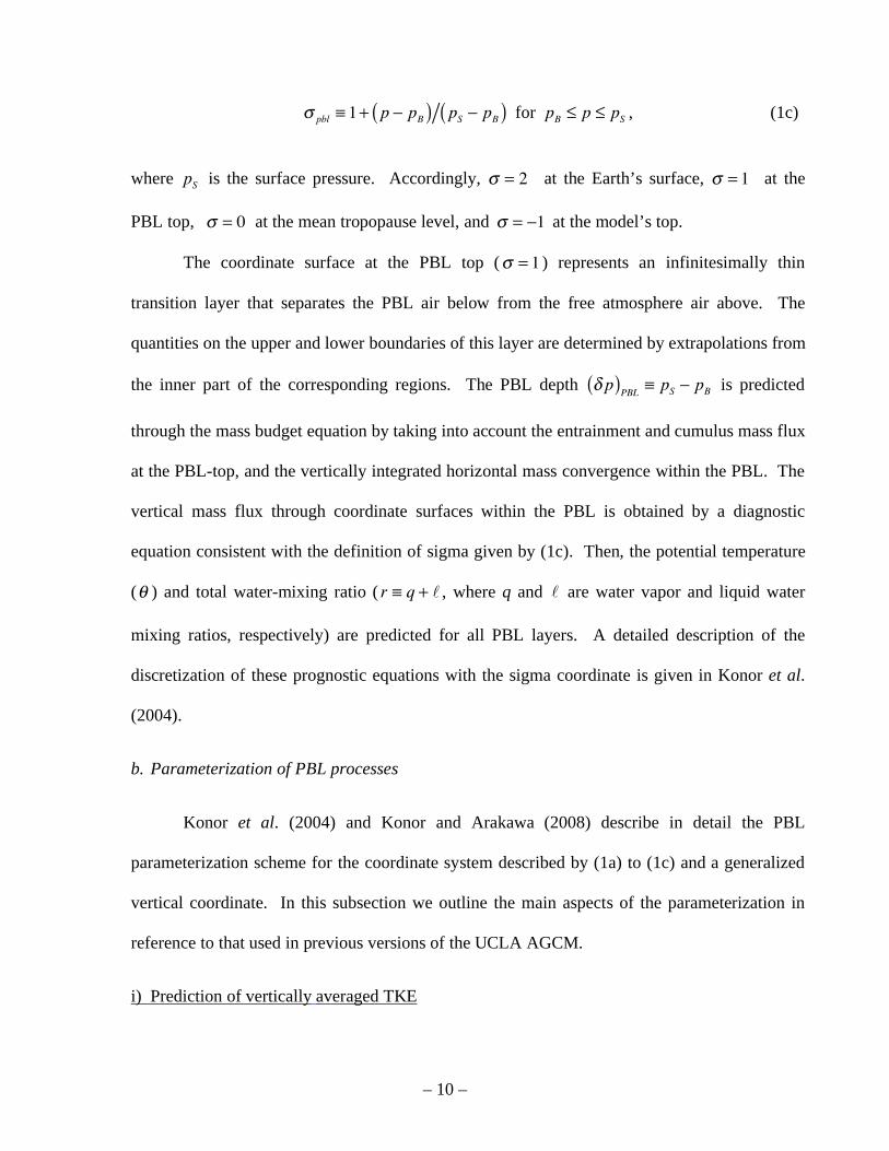
pbl 1+ p pB( ) pS pB( ) for pB p pS , (1c)

where pS is the surface pressure. Accordingly, = 2 at the Earth’s surface, = 1 at the

PBL top, = 0 at the mean tropopause level, and = 1 at the model’s top.

The coordinate surface at the PBL top ( = 1 ) represents an infinitesimally thin

transition layer that separates the PBL air below from the free atmosphere air above. The

quantities on the upper and lower boundaries of this layer are determined by extrapolations from

the inner part of the corresponding regions. The PBL depth p( )PBL pS pB is predicted

through the mass budget equation by taking into account the entrainment and cumulus mass flux

at the PBL-top, and the vertically integrated horizontal mass convergence within the PBL. The

vertical mass flux through coordinate surfaces within the PBL is obtained by a diagnostic

equation consistent with the definition of sigma given by (1c). Then, the potential temperature

( ) and total water-mixing ratio ( r q + , where q and are water vapor and liquid water

mixing ratios, respectively) are predicted for all PBL layers. A detailed description of the

discretization of these prognostic equations with the sigma coordinate is given in Konor et al.

(2004).

b. Parameterization of PBL processes

Konor et al. (2004) and Konor and Arakawa (2008) describe in detail the PBL

parameterization scheme for the coordinate system described by (1a) to (1c) and a generalized

vertical coordinate. In this subsection we outline the main aspects of the parameterization in

reference to that used in previous versions of the UCLA AGCM.

i) Prediction of vertically averaged TKE

– 11 –

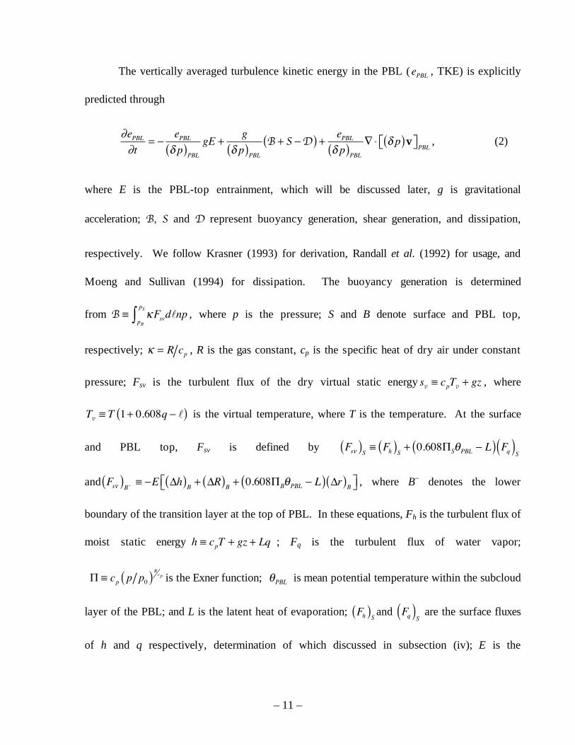
The vertically averaged turbulence kinetic energy in the PBL (ePBL , TKE) is explicitly

predicted through

ePBLt

=ePBLp( )PBL

gE +g

p( )PBLB + S D( ) +

ePBLp( )PBL

p( )vPBL

, (2)

where E is the PBL-top entrainment, which will be discussed later, g is gravitational

acceleration; B, S and D represent buoyancy generation, shear generation, and dissipation,

respectively. We follow Krasner (1993) for derivation, Randall et al. (1992) for usage, and

Moeng and Sullivan (1994) for dissipation. The buoyancy generation is determined

from

B Fsvd nppB

pS, where p is the pressure; S and B denote surface and PBL top,

respectively; = R cp , R is the gas constant, cp is the specific heat of dry air under constant

pressure; Fsv is the turbulent flux of the dry virtual static energy sv cpTv + gz , where

Tv T 1+ 0.608q( ) is the virtual temperature, where T is the temperature. At the surface

and PBL top, Fsv is defined by Fs( )S

Fh( )S+ 0.608 S PBL L( ) Fq( )

S

and Fs( )B–

E h( )B + R( )B + 0.608 B PBL L( ) r( )B , where B– denotes the lower

boundary of the transition layer at the top of PBL. In these equations, Fh is the turbulent flux of

moist static energy h cpT + gz + Lq ; Fq is the turbulent flux of water vapor;

cp p p0( )Rcp is the Exner function; PBL is mean potential temperature within the subcloud

layer of the PBL; and L is the latent heat of evaporation; Fh( )Sand Fq( )

S are the surface fluxes

of h and q respectively, determination of which discussed in subsection (iv); E is the

– 12 –

entrainment rate discussed in the next subsection; ( )B B+ Bis commonly called the

jump of at the PBL-top, where the subscript B+ upper boundary of the transition layer at the

top of PBL; R( )B is the radiation jump at the PBL top for a cloud-topped PBL. (Positive

values of the radiation jump correspond to radiative cooling.) The reader is referred to Konor

and Arakawa (2008), Suarez et al. (1983) and Randall (1976 and 1980b) for more details. To

summarize, the buoyancy generation includes the effects associated with the upward buoyancy

flux from the earth's surface through positive values of Fs( )S

and, in the case of a cloud-topped

PBL, the net long wave radiative cooling at the PBL top through positive values of R( )B ; the

buoyancy destruction includes the effects of entrainment of warmer and drier air from the free

atmosphere through positive values of E h( )B and the downward buoyancy flux from the

earth's surface through negative values of Fs( )S

. In our application of the TKE prediction

equation, we add the last term in (2) to represent a dilution (concentration) effect when PBL

deepens (shallows) due to horizontal mass convergence (divergence). It is assumed that the

predicted PBL TKE and depth cannot be lower than prescribed values

[ ePBL( )min

= 10 3m2sec 2 and pPBL( )min

= 10mb , respectively].

ii) Turbulent fluxes within the PBL

The turbulent fluxes are determined following a hybrid approach. For conserved

quantities, such as those of moist static energy h and total water mixing ratio r, turbulent fluxes

due to large eddies (with a length-scale of the order of PBL height) are determined from

– 13 –

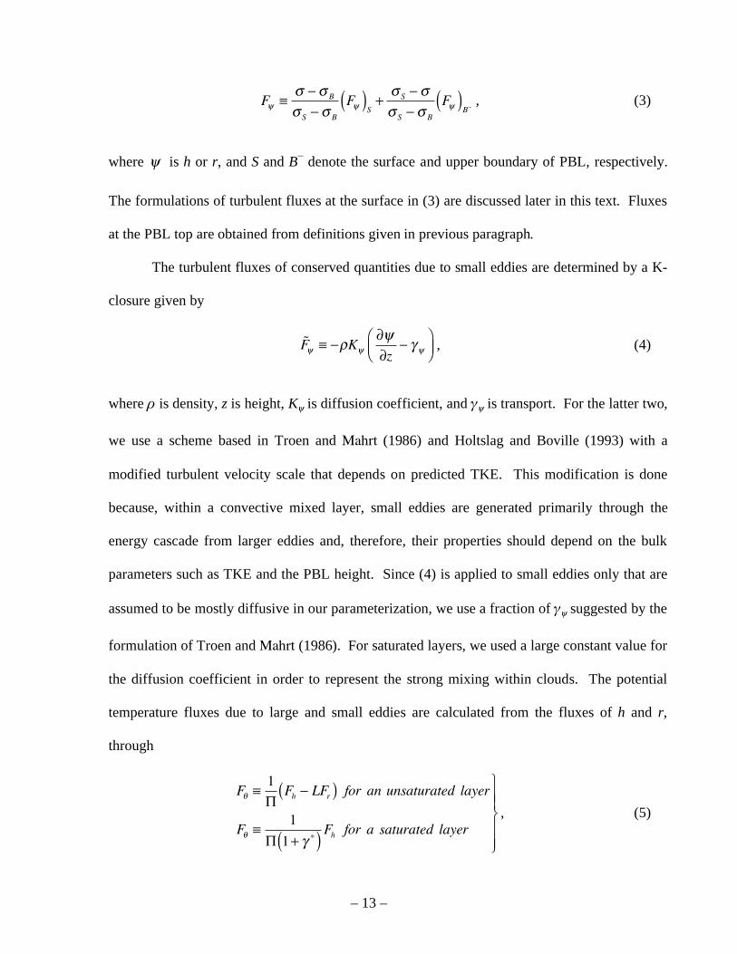
F B

S B

F( )S+ S

S B

F( )B

, (3)

where is h or r, and S and B– denote the surface and upper boundary of PBL, respectively.

The formulations of turbulent fluxes at the surface in (3) are discussed later in this text. Fluxes

at the PBL top are obtained from definitions given in previous paragraph.

The turbulent fluxes of conserved quantities due to small eddies are determined by a K-

closure given by

F Kz

, (4)

where is density, z is height, K is diffusion coefficient, and is transport. For the latter two,

we use a scheme based in Troen and Mahrt (1986) and Holtslag and Boville (1993) with a

modified turbulent velocity scale that depends on predicted TKE. This modification is done

because, within a convective mixed layer, small eddies are generated primarily through the

energy cascade from larger eddies and, therefore, their properties should depend on the bulk

parameters such as TKE and the PBL height. Since (4) is applied to small eddies only that are

assumed to be mostly diffusive in our parameterization, we use a fraction of suggested by the

formulation of Troen and Mahrt (1986). For saturated layers, we used a large constant value for

the diffusion coefficient in order to represent the strong mixing within clouds. The potential

temperature fluxes due to large and small eddies are calculated from the fluxes of h and r,

through

F1Fh LFr( ) for an unsaturated layer

F1

1+( )Fh for a saturated layer

, (5)

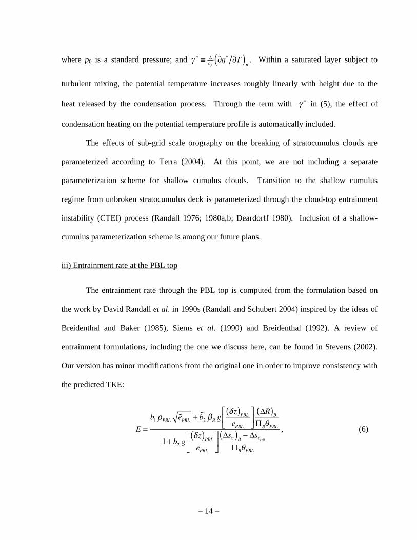
– 14 –

where p0 is a standard pressure; and Lcp

q T( )p. Within a saturated layer subject to

turbulent mixing, the potential temperature increases roughly linearly with height due to the

heat released by the condensation process. Through the term with in (5), the effect of

condensation heating on the potential temperature profile is automatically included.

The effects of sub-grid scale orography on the breaking of stratocumulus clouds are

parameterized according to Terra (2004). At this point, we are not including a separate

parameterization scheme for shallow cumulus clouds. Transition to the shallow cumulus

regime from unbroken stratocumulus deck is parameterized through the cloud-top entrainment

instability (CTEI) process (Randall 1976; 1980a,b; Deardorff 1980). Inclusion of a shallow-

cumulus parameterization scheme is among our future plans.

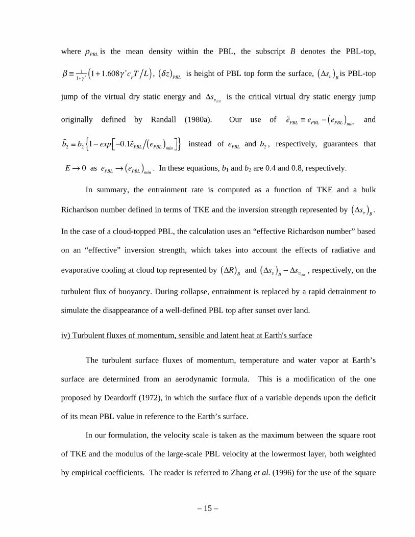
iii) Entrainment rate at the PBL top

The entrainment rate through the PBL top is computed from the formulation based on

the work by David Randall et al. in 1990s (Randall and Schubert 2004) inspired by the ideas of

Breidenthal and Baker (1985), Siems et al. (1990) and Breidenthal (1992). A review of

entrainment formulations, including the one we discuss here, can be found in Stevens (2002).

Our version has minor modifications from the original one in order to improve consistency with

the predicted TKE:

E =

b1 PBL ePBL + b2 B gz( )PBLePBL

R( )BB PBL

1+ b2 gz( )PBLePBL

sv( )B

svcrit

B PBL

, (6)

– 15 –

where PBL is the mean density within the PBL, the subscript B denotes the PBL-top,

1

1+1+1.608 cpT L( ) , z( )PBL is height of PBL top form the surface, sv( )

Bis PBL-top

jump of the virtual dry static energy and svcrit is the critical virtual dry static energy jump

originally defined by Randall (1980a). Our use of ePBL ePBL ePBL( )

min and

b2 b2 1 exp 0.1ePBL ePBL( )

min{ } instead of ePBL and b2 , respectively, guarantees that

E 0 as ePBL ePBL( )min

. In these equations, b1 and b2 are 0.4 and 0.8, respectively.

In summary, the entrainment rate is computed as a function of TKE and a bulk

Richardson number defined in terms of TKE and the inversion strength represented by sv( )B

.

In the case of a cloud-topped PBL, the calculation uses an “effective Richardson number” based

on an “effective” inversion strength, which takes into account the effects of radiative and

evaporative cooling at cloud top represented by R( )B and sv( )B

svcrit, respectively, on the

turbulent flux of buoyancy. During collapse, entrainment is replaced by a rapid detrainment to

simulate the disappearance of a well-defined PBL top after sunset over land.

iv) Turbulent fluxes of momentum, sensible and latent heat at Earth's surface

The turbulent surface fluxes of momentum, temperature and water vapor at Earth’s

surface are determined from an aerodynamic formula. This is a modification of the one

proposed by Deardorff (1972), in which the surface flux of a variable depends upon the deficit

of its mean PBL value in reference to the Earth’s surface.

In our formulation, the velocity scale is taken as the maximum between the square root

of TKE and the modulus of the large-scale PBL velocity at the lowermost layer, both weighted

by empirical coefficients. The reader is referred to Zhang et al. (1996) for the use of the square

– 16 –

root of TKE as the velocity scale in the surface flux formulation. The surface fluxes obtained in

this way are expected to be better than those obtained with more traditional methods in regions

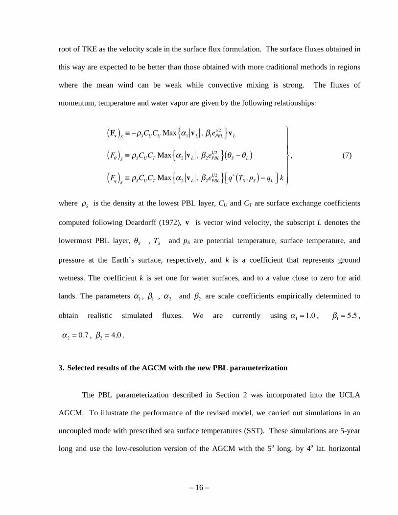
where the mean wind can be weak while convective mixing is strong. The fluxes of

momentum, temperature and water vapor are given by the following relationships:

Fv( )S SCUCUMax 1 vL , 1ePBL

1 2{ }vL

F( )S SCUCT Max 2 vL , 2ePBL

1 2{ } S L( )

Fq( )S SCUCT Max 2 vL , 2ePBL

1 2{ } q TS , pS( ) qL k

, (7)

where S is the density at the lowest PBL layer, CU and CT are surface exchange coefficients

computed following Deardorff (1972), v is vector wind velocity, the subscript L denotes the

lowermost PBL layer, S , TS and pS are potential temperature, surface temperature, and

pressure at the Earth’s surface, respectively, and k is a coefficient that represents ground

wetness. The coefficient k is set one for water surfaces, and to a value close to zero for arid

lands. The parameters 1 , 1 , 2 and 2 are scale coefficients empirically determined to

obtain realistic simulated fluxes. We are currently using 1 = 1.0 , 1 = 5.5 ,

2 = 0.7 , 2 = 4.0 .

3. Selected results of the AGCM with the new PBL parameterization

The PBL parameterization described in Section 2 was incorporated into the UCLA

AGCM. To illustrate the performance of the revised model, we carried out simulations in an

uncoupled mode with prescribed sea surface temperatures (SST). These simulations are 5-year

long and use the low-resolution version of the AGCM with the 5o long. by 4

o lat. horizontal

– 17 –

resolution with 18 layers (4 in the PBL). The initial condition corresponds to November 30 in a

long-term run of a previous model version with the same resolution, but using a single-layer

PBL. The SST, sea-ice, Earth’s surface albedo and roughness, and ground wetness distributions

are obtained daily by linear interpolation from the twelve monthly means of observed

climatologies taken from the Global Sea-Ice and SST Data Set (Rayner et al. 1995) for sea-ice

and SST, and Dorman and Sellers (1989) for surface albedo and roughness. We show the

averages of monthly means over a 5-year period. Our emphasis in this section is on those fields

that are directly influenced by the PBL scheme.

a. Global surface fields

We start by inspecting the simulated monthly-mean sea level pressure. Figure 3 shows

the distributions for January and July (left and right columns, respectively) from the NCEP

reanalysis (Kalnay et al. 1996) and the simulation (upper and lower rows, respectively). The

simulation clearly reproduces the main features of the observed climatology, such as the

subtropical highs in the Northern Hemisphere during summer, the Aleutian low during winter,

and the subtropical highs in the Southern Hemisphere both in winter and summer. In January,

the simulated sea level pressure over the continents in the Northern Hemisphere tends to be

lower than in the NCEP reanalysis. Note that the differences between the observation and

simulation over Tibetan plateau are influenced by the method used to obtain sea level values in

regions of high terrain. The simulated low-pressure belt around Antarctica is too weak in both

January and July, which is a feature fairly common to AGCMs with low horizontal resolution

(Boville 1991).

Figure 4 shows the simulated monthly-mean PBL depth, TKE, and stratocumulus clouds

incidence (as the percentage of time of occurrence) for January, April, July and October. The

– 18 –

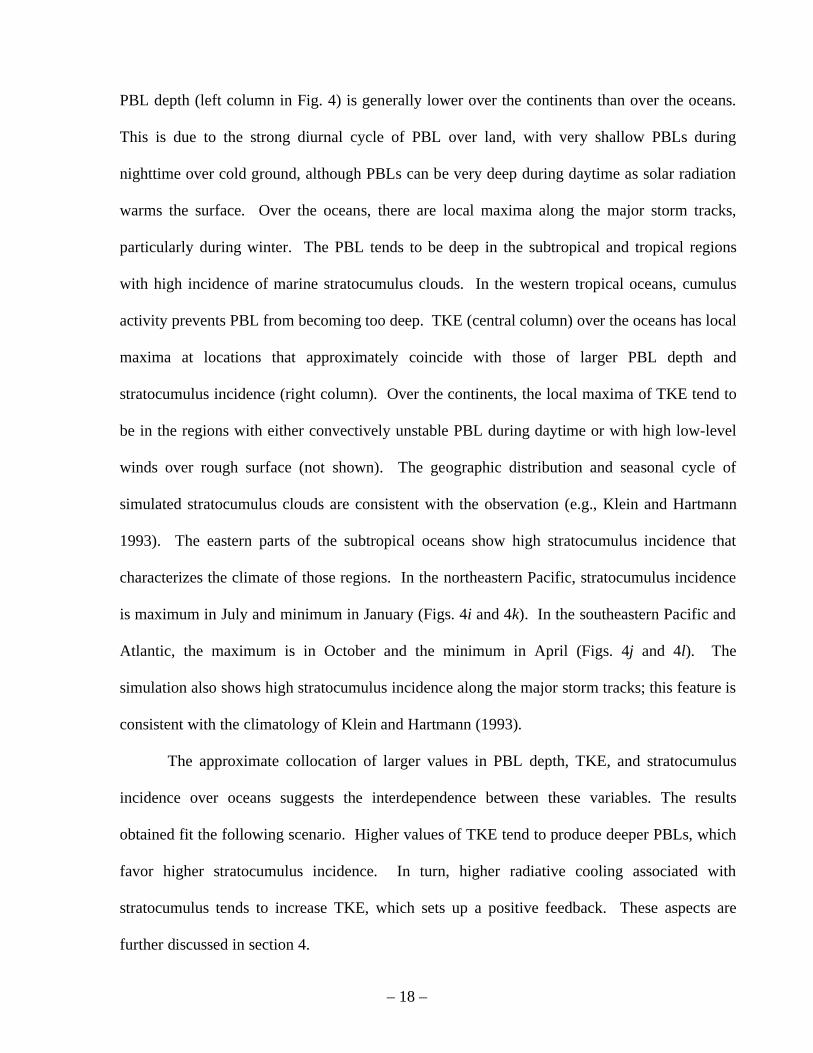
PBL depth (left column in Fig. 4) is generally lower over the continents than over the oceans.

This is due to the strong diurnal cycle of PBL over land, with very shallow PBLs during

nighttime over cold ground, although PBLs can be very deep during daytime as solar radiation

warms the surface. Over the oceans, there are local maxima along the major storm tracks,

particularly during winter. The PBL tends to be deep in the subtropical and tropical regions

with high incidence of marine stratocumulus clouds. In the western tropical oceans, cumulus

activity prevents PBL from becoming too deep. TKE (central column) over the oceans has local

maxima at locations that approximately coincide with those of larger PBL depth and

stratocumulus incidence (right column). Over the continents, the local maxima of TKE tend to

be in the regions with either convectively unstable PBL during daytime or with high low-level

winds over rough surface (not shown). The geographic distribution and seasonal cycle of

simulated stratocumulus clouds are consistent with the observation (e.g., Klein and Hartmann

1993). The eastern parts of the subtropical oceans show high stratocumulus incidence that

characterizes the climate of those regions. In the northeastern Pacific, stratocumulus incidence

is maximum in July and minimum in January (Figs. 4i and 4k). In the southeastern Pacific and

Atlantic, the maximum is in October and the minimum in April (Figs. 4j and 4l). The

simulation also shows high stratocumulus incidence along the major storm tracks; this feature is

consistent with the climatology of Klein and Hartmann (1993).

The approximate collocation of larger values in PBL depth, TKE, and stratocumulus

incidence over oceans suggests the interdependence between these variables. The results

obtained fit the following scenario. Higher values of TKE tend to produce deeper PBLs, which

favor higher stratocumulus incidence. In turn, higher radiative cooling associated with

stratocumulus tends to increase TKE, which sets up a positive feedback. These aspects are

further discussed in section 4.

– 19 –

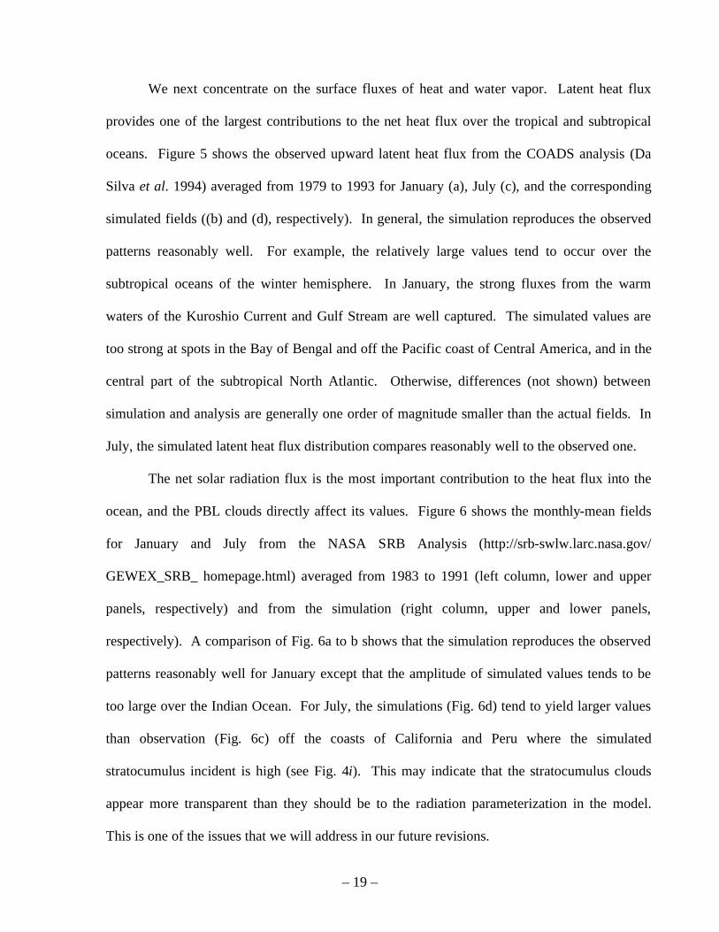
We next concentrate on the surface fluxes of heat and water vapor. Latent heat flux

provides one of the largest contributions to the net heat flux over the tropical and subtropical

oceans. Figure 5 shows the observed upward latent heat flux from the COADS analysis (Da

Silva et al. 1994) averaged from 1979 to 1993 for January (a), July (c), and the corresponding

simulated fields ((b) and (d), respectively). In general, the simulation reproduces the observed

patterns reasonably well. For example, the relatively large values tend to occur over the

subtropical oceans of the winter hemisphere. In January, the strong fluxes from the warm

waters of the Kuroshio Current and Gulf Stream are well captured. The simulated values are

too strong at spots in the Bay of Bengal and off the Pacific coast of Central America, and in the

central part of the subtropical North Atlantic. Otherwise, differences (not shown) between

simulation and analysis are generally one order of magnitude smaller than the actual fields. In

July, the simulated latent heat flux distribution compares reasonably well to the observed one.

The net solar radiation flux is the most important contribution to the heat flux into the

ocean, and the PBL clouds directly affect its values. Figure 6 shows the monthly-mean fields

for January and July from the NASA SRB Analysis (http://srb-swlw.larc.nasa.gov/

GEWEX_SRB_ homepage.html) averaged from 1983 to 1991 (left column, lower and upper

panels, respectively) and from the simulation (right column, upper and lower panels,

respectively). A comparison of Fig. 6a to b shows that the simulation reproduces the observed

patterns reasonably well for January except that the amplitude of simulated values tends to be

too large over the Indian Ocean. For July, the simulations (Fig. 6d) tend to yield larger values

than observation (Fig. 6c) off the coasts of California and Peru where the simulated

stratocumulus incident is high (see Fig. 4i). This may indicate that the stratocumulus clouds

appear more transparent than they should be to the radiation parameterization in the model.

This is one of the issues that we will address in our future revisions.

– 20 –

b. Vertical Profiles of Thermodynamic Variables over Ocean

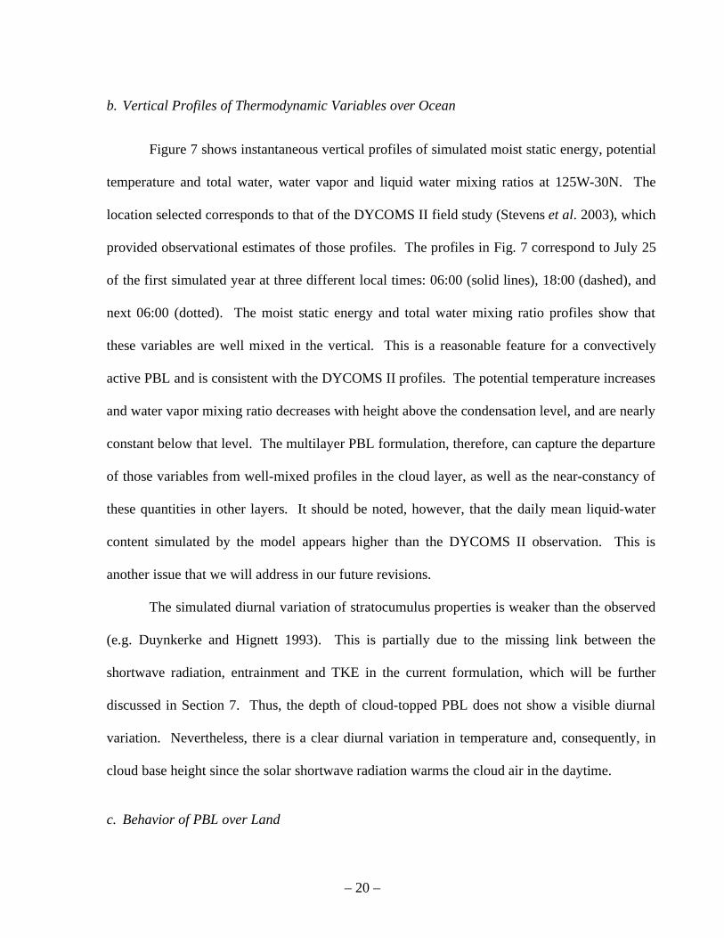
Figure 7 shows instantaneous vertical profiles of simulated moist static energy, potential

temperature and total water, water vapor and liquid water mixing ratios at 125W-30N. The

location selected corresponds to that of the DYCOMS II field study (Stevens et al. 2003), which

provided observational estimates of those profiles. The profiles in Fig. 7 correspond to July 25

of the first simulated year at three different local times: 06:00 (solid lines), 18:00 (dashed), and

next 06:00 (dotted). The moist static energy and total water mixing ratio profiles show that

these variables are well mixed in the vertical. This is a reasonable feature for a convectively

active PBL and is consistent with the DYCOMS II profiles. The potential temperature increases

and water vapor mixing ratio decreases with height above the condensation level, and are nearly

constant below that level. The multilayer PBL formulation, therefore, can capture the departure

of those variables from well-mixed profiles in the cloud layer, as well as the near-constancy of

these quantities in other layers. It should be noted, however, that the daily mean liquid-water

content simulated by the model appears higher than the DYCOMS II observation. This is

another issue that we will address in our future revisions.

The simulated diurnal variation of stratocumulus properties is weaker than the observed

(e.g. Duynkerke and Hignett 1993). This is partially due to the missing link between the

shortwave radiation, entrainment and TKE in the current formulation, which will be further

discussed in Section 7. Thus, the depth of cloud-topped PBL does not show a visible diurnal

variation. Nevertheless, there is a clear diurnal variation in temperature and, consequently, in

cloud base height since the solar shortwave radiation warms the cloud air in the daytime.

c. Behavior of PBL over Land

– 21 –

In this subsection, we focus on January (austral summer) and select two locations over

land corresponding to moist and semi-arid soil. On these locations, therefore, we expect the

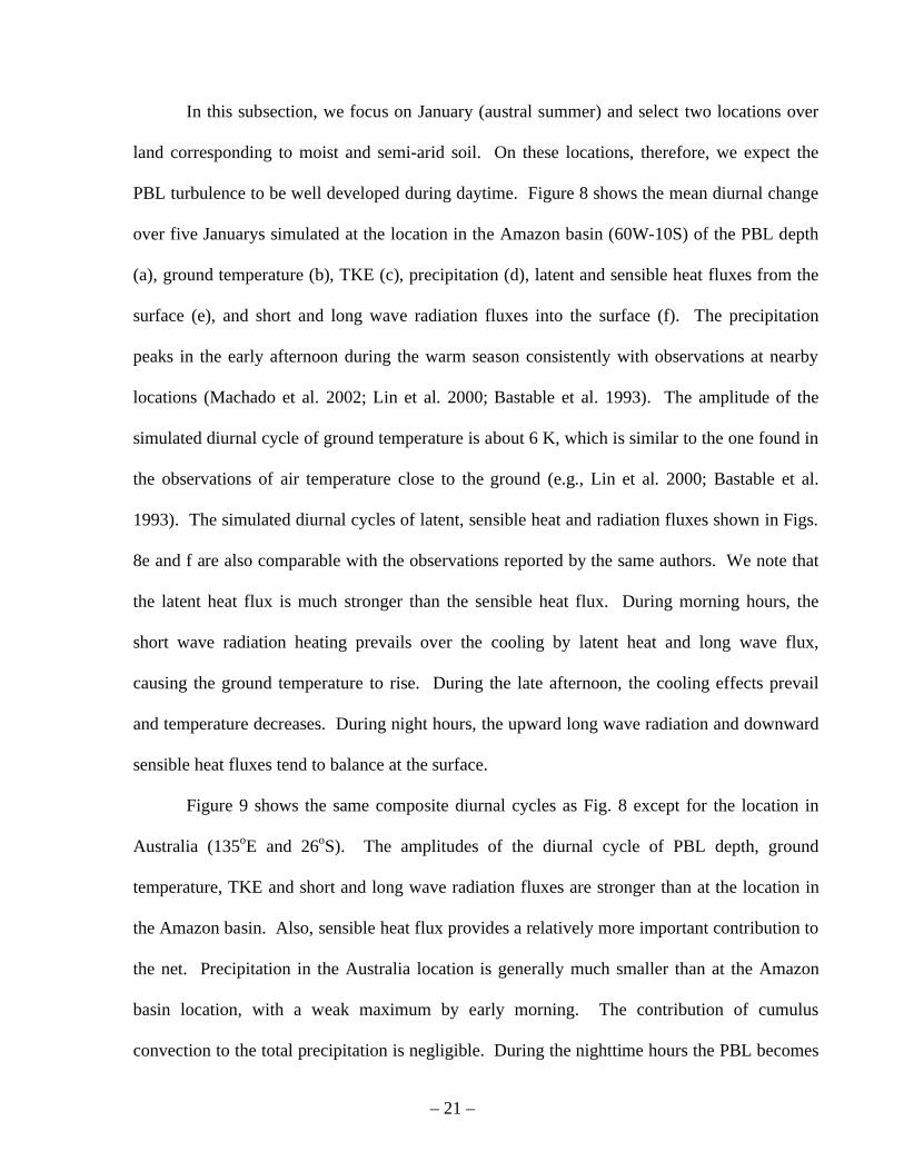
PBL turbulence to be well developed during daytime. Figure 8 shows the mean diurnal change

over five Januarys simulated at the location in the Amazon basin (60W-10S) of the PBL depth

(a), ground temperature (b), TKE (c), precipitation (d), latent and sensible heat fluxes from the

surface (e), and short and long wave radiation fluxes into the surface (f). The precipitation

peaks in the early afternoon during the warm season consistently with observations at nearby

locations (Machado et al. 2002; Lin et al. 2000; Bastable et al. 1993). The amplitude of the

simulated diurnal cycle of ground temperature is about 6 K, which is similar to the one found in

the observations of air temperature close to the ground (e.g., Lin et al. 2000; Bastable et al.

1993). The simulated diurnal cycles of latent, sensible heat and radiation fluxes shown in Figs.

8e and f are also comparable with the observations reported by the same authors. We note that

the latent heat flux is much stronger than the sensible heat flux. During morning hours, the

short wave radiation heating prevails over the cooling by latent heat and long wave flux,

causing the ground temperature to rise. During the late afternoon, the cooling effects prevail

and temperature decreases. During night hours, the upward long wave radiation and downward

sensible heat fluxes tend to balance at the surface.

Figure 9 shows the same composite diurnal cycles as Fig. 8 except for the location in

Australia (135oE and 26

oS). The amplitudes of the diurnal cycle of PBL depth, ground

temperature, TKE and short and long wave radiation fluxes are stronger than at the location in

the Amazon basin. Also, sensible heat flux provides a relatively more important contribution to

the net. Precipitation in the Australia location is generally much smaller than at the Amazon

basin location, with a weak maximum by early morning. The contribution of cumulus

convection to the total precipitation is negligible. During the nighttime hours the PBL becomes

– 22 –

very shallow. During the daytime hours, the high sensible heat flux from the ground contributes

to increase TKE and, therefore, the PBL depth.

d. Comparison of the AGCM performance with the new and previous PBL parameterizations

To assess the impact of the new scheme, we compare the simulation described in the

previous subsection with another that uses the previous version of the PBL parameterization

(hereafter SP simulation). The reader is referred to Suarez et al. (1983) for a detailed

description of that previous version. In short, the previous parameterization treats the PBL as a

well-mixed single layer, the entrainment rate is determined by solving an implicit equation, and

the aerodynamic formulas to determine the surface fluxes use mean PBL wind as velocity scale.

The implicit equation that determines the entrainment rate is obtained by neglecting the time

derivative term in a TKE budget equation similar to (2). A complex iteration procedure

discussed by Suarez et al. (1983) is used to solve the resulting equation for the entrainment rate.

This parameterization has two potential shortcomings in comparison to the new

parameterization, first of which is that neglecting the time derivative of TKE in the TKE budget

eliminates the transient behavior of PBL. The second is that there is no room to directly

implement physical processes for entrainment beyond the equilibrium of TKE.

Figure 10 shows the January- and July-mean PBL depth (a and b, respectively) and

stratocumulus incident (c and d, respectively) in the SP simulation. A comparison with Control

(Fig. 4) shows that the new parameterization generates more detailed PBL depth patterns (Fig

4a for January and g for July) and a better seasonal variability of stratocumulus incidence (Fig.

4c for January and i for July), particularly in the stratocumulus regions. Fig. 11 shows the

January- and July-mean net latent heat fluxes at the surface in SP simulation. Overall, upward

fluxes in SP simulation are larger than in the observation (Fig. 5a for January and c for July)

– 23 –

and Control (Fig. 5b for January and d for July). The overall pattern of the fluxes in the

southern Tropics in July is less zonal than the observation and Control. Over the eastern

Pacific, however, the new formulation gives higher values than the observation and SP

simulation. The monthly-mean net shortwave radiation fluxes at the surface for the same

months in the SP simulation (Fig. 12a and b) compares reasonably well with both the observed

(Fig. 6a and c) and Control (Fig. 6b and d). There is, nevertheless, a small improvement with

the new parameterization over the Southern Hemisphere Atlantic and Pacific Oceans in January.

It is clear from these comparisons that the new PBL parameterization has overall significantly

improved the estimation of the surface latent heat flux in our GCM. Moderate to small

improvements are also achieved in the simulation of seasonal variability of stratocumulus

incidence and the estimates of net shortwave radiation flux at the surface. We attribute a large

part of these improvements to the explicit prediction of TKE and its use in the determination of

entrainment rate and surface fluxes in the new PBL parameterization. The overall improvement

of the simulated surface latent heat fluxes with the new parameterization is primarily due to the

use of the square root of TKE as a velocity scale in the aerodynamical formula for the surface

flux. Particularly in the Tropics, where the mean PBL wind is weak, the surface fluxes are

controlled by the subgrid scale convective activity, which is well represented by the bulk TKE.

e. Comparison of simulated baroclinic activity with multi- and single-layer PBL

parameterizations

In the introduction we stated that explicit prediction of vertical shears within the PBL

could have an impact on the evolution of extratropical baroclinic disturbances. To examine this

potential impact we select the poleward heat transport near the surface (i.e., within the PBL) in

synoptic time scales as a proxy for baroclinic eddy activity. Then, we compare the values for

our baroclinic activity to the one obtained by a version of the same AGCM, in which the

– 24 –

number of layers for the PBL is set to one. Otherwise, these two versions of the model are

identical.

Figure 13 shows the mean January (upper panel, a and b) and July (lower panel, c and d)

latitudinal poleward potential temperature flux by eddies ( v ) within the PBL, where prime

indicates deviation from the zonal mean, from the CONTROL (left column) and the single-layer

simulation (right column). (The values for the CONTROL correspond to vertical averages

within the PBL.) To focus on the synoptic scale baroclinic activity, a band-pass filter between 3

and 8 days is applied. A comparison of the panels (a) and (c) to (b) and (d) of Fig. 13,

respectively, indicates that the multi-layer scheme generally yields higher baroclinic activity

implied by the magnitude of (v ) than the single-layer scheme does. It should be noted that

the horizontal resolutions we are using are insufficient to properly resolve the details of synoptic

scale eddies. Nevertheless, our comparison still indicates that the use of multiple layers in the

PBL produces a more realistic level of baroclinic activity.

f. Performance of the AGCM coupled to an OGCM

We have also performed simulations in which the AGCM coupled to a near global MIT-

OGCM. [The reader is referred to Cazes-Boezio et al. (2005) for the coupled model results.]

Experiments in the coupled mode is a necessary task to validate AGCMs since prescribing SSTs

in the uncoupled mode assumes the most important part of the answer and, therefore, it may

hide crucial deficiencies of the model.

In the coupled simulations, the SST field (not shown) demonstrates several realistic

features both in terms of annual means (such as realistic equatorial SST gradients in both

Pacific and Atlantic basins) and interannual variability (such as ENSO-like anomalies in SST

and the atmospheric circulation). The outstandingly successful feature of the simulations is that

– 25 –

the extent and seasonal cycle of stratocumulus clouds and their effects on short wave radiation

and SST in the eastern part of the subtropical oceans are well simulated. We attribute a large

part of this success to the merits of our PBL framework.

4. Importance of interactions between radiation and turbulence in a cloud-topped PBL

In this section we examine the importance of radiation, turbulence and thermodynamics

interactions in the PBL when stratocumulus clouds are present. The radiative cooling at the

PBL top is of fundamental importance for the generation of TKE and turbulence fluxes in a

cloud-topped PBL. In the formulation we are presenting here, the PBL top coincides with that

of stratocumulus clouds. Hence, the radiation calculation in the AGCM directly gives the value

of radiative cooling at the PBL top, which is then explicitly included in the formulations of the

TKE generation, PBL-top mass entrainment, and the time derivative of potential temperature of

the uppermost PBL layer. In our model, therefore, the importance of this cooling can easily be

assessed by an experiment in which this effect is neglected.

We focus on July, during which the high incidence of stratocumulus in the eastern parts

of tropical and subtropical oceans is generally well captured by the AGCM (see Fig. 2). We

start by performing a simulation in which radiative cooling at the PBL top is set to zero in the

calculation of TKE and mass entrainment, but kept in the potential temperature prediction

(hereafter “NR1 simulation”). Note that the radiative cooling affects the TKE budget through

the buoyancy generation as discussed in subsection 2b (i). The impact of its overall effect can

be seen in the differences between the NR simulation and that presented in Section 3 (hereafter

“Control”). Figure 14 shows TKE, PBL depth and stratocumulus incidence from the NR1

simulation (Fig. 14a, c and e, respectively) and the differences from the Control (NR1

simulation–Control) (Figs. 4h, g and i). In the eastern parts of the subtropical and tropical

– 26 –

oceans, regions in which stratocumulus incidence obtained in the Control is high, the PBL

depth, TKE and stratocumulus incidence are reduced in the NR1 simulation. Off the coast of

California, the reduction is as high as 60%, while off the coasts of Peru and Namibia the

reduction is about 30%. The lack of radiative cooling effect at the PBL reduces the TKE and

entrainment rate in the stratocumulus region, and thus the PBL becomes shallower. A positive

feedback is established as the PBL top lowers and condensation level rises. Along the North

Pacific storm track, both the NR1 simulations and Control show a very shallow PBL (Figs. 4g

and 14c), low TKE, and high stratocumulus incidence (Figs. 4i and 13e). In this region, PBL is

usually stable. In such a situation, the lower entrainment rate produces higher incidence of fog

since the mixing of air between the PBL and the overlying drier free atmosphere is reduced.

Despite the lower incidence of stratocumulus clouds in the eastern parts of subtropical

and tropical regions in the NR1 simulation, there are still local maxima of PBL depth in these

regions. This is partially due to the TKE generation by the upward surface heat fluxes resulting

from low-level cold advection from higher latitudes along the eastern branch of the subtropical

anticyclones. In addition, the radiative cooling of the cloud layer is still active in the NR1

simulation.

To completely eliminate the effects of radiative cooling that influences the PBL, we set

the radiative cooling to zero both in the calculation of TKE and mass entrainment and in the

potential temperature prediction in the uppermost PBL layer. We call this experiment NR2. In

this experiment, the stratocumulus incidence for July (see Fig. 15) is further reduced from the

NR1 simulation (Fig. 14) to the point of almost vanishing even in the regions where they are

most persistent in the Control (Fig. 4).

A comparison of the results of NR1 and NR2 experiments reveals that the cooling of the

PBL air due to the cloud-top radiative cooling indirectly contributes to the budget of TKE (and

– 27 –

therefore entrainment rate) and helps, to a certain degree, maintenance of stratocumulus decks

over oceans. The indirect link is through the enhanced surface heat fluxes (and, therefore,

through the buoyancy contribution to TKE) caused by the cooler PBL air under the clouds.

This indicates the existence of a feedback process between the PBL clouds and surface heat

fluxes.

5. Comparison with models with the traditional vertical structure

In the previous section, we presented a comparison to assess the effect of processes

associated with stratocumulus clouds on the turbulence fluxes using the new framework. To

what degree the lack of these processes in a model with a traditional PBL parameterization

influences the simulations is an interesting question. There have been many studies that

combine a traditional parameterization with interactive cloud parameterizations beyond

diagnostic treatments (e.g., Soares et al., 2004; Lock et al., 2000). In this paper, however, what

we mean with the traditional PBL parameterization is a parameterization characterized by two

aspects. One is the use of the “traditional” vertical structure, in which the vertical coordinate is

a terrain following sigma type. As mentioned earlier, we use a different vertical structure, in

which the PBL has its own multiple layers with predicted depth. In an early version of the

UCLA GCM, an attempt was made to incorporate a mixed-layer based PBL parameterization,

with a traditional vertical structure (Randall, 1976). Not having the PBL top coinciding with a

coordinate surface in the traditional vertical structure made the PBL-top jump very difficult to

determine and caused the abandonment of this attempt later (Suarez et al., 1983). This

experience is an indication that the vertical structure we use is paramount for a successful

incorporation of the new PBL parameterization to our model. The second aspect of what we

mean by the traditional parameterization is the use of diagnostically determined PBL clouds

– 28 –

without formulation of their effects in the parameterization itself. We use such a

parameterization to see the difference between prognostic and diagnostic determinations of

clouds in a simple context.

How the results obtain by a model with the traditional PBL parameterization compare to

those presented in section 3 is examined here. For this purpose we constructed a version of our

model with the traditional vertical structure. To do that, first we replace the part of the vertical

coordinate given by (1b) and (1c) for pI p pS by a conventional sigma coordinate such as

the one defined as trop 2 p pI( ) pS pI( ) . Note that the total number of model layers is

kept the same as in the Control. For the PBL parameterization, we choose the scheme used by

Holtslag and Boville (1993). The scheme requires a definition of the PBL depth, for which we

choose the diagnostic expression using a bulk Richardson number introduced by Troen and

Mahrt (1986). In this experiment, we diagnose the PBL depth at each dynamics time step. To

diagnose the PBL clouds, we calculated the lifting level of condensation (LLC). If the LLC is

below the PBL-top height, it is assumed that the PBL is topped with stratocumulus clouds.

Figure 16 shows the July-mean distribution of the PBL depth, stratocumulus incidence

diagnosed for the PBL and low-level cloud incidence simulated by this experiment, which we

call the fixed-sigma simulation. The low-level cloud incidence (cloud incidence for the lowest

250 mb deep portion of the troposphere) is presented because the stratocumulus clouds

incidence diagnosed for the PBL may not fully represent the clouds resulted from the PBL

processes in the fixed-sigma simulation. In the subtropical oceans, the distributions of

maximum and minimum of the PBL depth distribution (Fig. 16a) are almost opposite to those in

the Control (Fig. 4g). In the fixed-sigma experiment, the regions of the observed high incidence

of marine stratocumulus off the coasts of California, Peru and Namibia show relative minima of

– 29 –

PBL depth while those in the western parts of the oceans show relative maxima. Altogether, the

patterns in Fig. 16a are very unrealistic. The incidence of stratocumulus clouds tends to have

relative maxima in the western parts of the oceans in the fixed-sigma experiment while relative

maxima appear in the eastern parts of the oceans in the Control. The stratocumulus incidence in

the low-pressure belt around Antarctica is relatively well simulated, but it has a more zonal

pattern than in the Control. The low-level cloud incidence for July shown in Fig. 16c is overall

unrealistically high almost everywhere, and tends to have relative minima in the usual marine

stratocumulus regions.

We interpret the differences between the results presented in Fig. 16 and the Control as

the results of two main deficiencies in the fixed-sigma model. First, the formula that determines

the PBL depth is diagnostic without considering the mass budget. Second, the processes at the

cloud top that influence the turbulent fluxes are absent. According to the diagnostic equation

that determines the PBL depth in the fixed-sigma model, the surface heat flux and the mean

shear are the two main controllers of the PBL depth (The higher the upward flux is and/or the

stronger the shear is, the deeper the PBL is.) In the fixed-sigma simulation, therefore, the PBL

tends to be deeper in the areas with high SSTs. Only when the PBL is deep enough, the

stratocumulus clouds can be maintained regardless of the processes associated with these

clouds. In this sense, it is not surprising that the important features of the marine PBL are

poorly simulated in the fixed-sigma experiment.

6. Summary and Discussions

In this paper, we present the basic features and an assessment of a newly developed PBL

parameterization scheme implemented in the UCLA AGCM. The new scheme maintains many

features of the previous PBL schemes of the UCLA AGCM (Suarez et al. 1983). These

– 30 –

features can be summarized as follows: the depth of PBL is predicted through the mass budget

for the PBL including the entrainment through its top, the cumulus mass flux and the vertically

integrated horizontal mass flux convergence. Within the PBL a modified sigma coordinate is

used, in which the PBL and free atmosphere share a coordinate surface at the PBL top. The

PBL top then becomes a material surface in the absence of entrainment (or detrainment) and

cumulus mass flux. The new PBL scheme uses multiple layers within the PBL as opposed to

the single layer in the previous schemes. The vertically integrated turbulence kinetic energy

(TKE) is predicted through a kinetic energy budget equation including the buoyancy and shear

generation, dilution due to the PBL-top mass entrainment, and dissipation. The buoyancy

generation includes the effects of the upward surface heat fluxes and radiative cooling at the

cloud top (PBL-top and cloud top coincide if the PBL is cloudy). The PBL top entrainment is

determined from a formulation that takes into account the effects of TKE and the radiative and

evaporative cooling concentrated near the PBL top (Randall and Schubert 2004). The surface

fluxes are determined from an aerodynamic formula, in which a combination of the square root

of TKE and the grid-scale surface wind are used to represent the velocity scale. The turbulent

fluxes within the PBL are determined through an approach considering the effects of both large

convective and small diffusive eddies through bulk and K-closure formulations, respectively.

Using these fluxes, we explicitly predict the vertical profiles of the variables.

To illustrate the performance of the model with the new PBL parameterization, we

carried out simulations in an uncoupled mode with prescribed SST and in a coupled mode using

a near global MIT-OGCM. In this paper, we present the results from the uncoupled

simulations. Monthly-mean fields of the simulated SLP, PBL height, TKE, stratocumulus

incidence, and net solar radiation and latent heat fluxes at the surface are shown. These fields

(except PBL height and TKE, for which observations are not available) match reasonably well

– 31 –

to their observed counterparts. The distribution and seasonal variation of the stratocumulus

incidence off the coasts of California, Peru and Namibia are realistic. A comparison of these

results to the ones obtained by using the previous version of the PBL parameterization

demonstrates an overall improvement in the simulations with the new parameterization. The

simulated PBL profiles near the location of DYCOMS II field experiment demonstrate the same

major features of the observed profiles. The composite diurnal cycles of various fields

including PBL depth and precipitation over moist and semi-arid land points are also examined.

Over a semi-arid land point, the PBL reaches its maximum depth late afternoon just before

sunset and crashes rapidly after sunset completing a cycle as observed in nature. Over moist

land (a point chosen in the Amazon region), the diurnal cycle of precipitation shows

precipitation peaks in the afternoon as observed.

Simulation of the formation and maintenance of the marine stratocumulus decks off the

coasts of California, Peru and Namibia presents a real challenge for climate models. Success of

the model generally depends on the formulation of the interactions between radiation,

turbulence and thermodynamics in the cloud-topped PBL. While the results presented in section

3 confirm the overall effectiveness and realism of the parameterized PBL processes with the

new formulation, we additionally performed experiments to demonstrate the important role of

these interactions in maintaining marine stratocumulus decks. We first eliminated the

turbulence and radiative cooling interaction by setting the radiative cooling to zero in the

buoyancy generation of TKE and in the entrainment formula. The results obtained from this

experiment are very different from those of the control simulation. In the usual stratocumulus

regions, the simulated cloud incidence is drastically reduced and the PBL becomes shallower

and less turbulent compared to the Control. As an extension of this experiment, the radiative

cooling effect is also removed from the potential temperature equation for the uppermost PBL

– 32 –

layer. The simulation from this experiment virtually eliminates already infrequent

stratocumulus incidence. These two experiments indicate that it is very difficult to maintain the

clouds against the destructive effects of subsidence prevailing in these regions without properly

simulating the cloud radiative cooling, turbulence and temperature interactions.

We also examine whether the AGCM would yield very different results if a PBL

parameterization based on the formulation described by Holtslag and Boville (1993) is used.

For this purpose, we modify the model to use the conventional sigma coordinate and determine

the PBL height using the formula introduced by Troen and Mahrt (1986) and used by Holtslag

and Boville (1993). The results are significantly worse than the Control particularly for the

stratocumulus incidence over the oceans. This comparison also confirms the importance of

cloud radiation-turbulence interaction processes in the PBL parameterization for realistic

simulations of the stratocumulus clouds.

In the coupled simulations (not shown here), the SST field illustrates realistic equatorial

SST gradients in both Pacific and Atlantic basins both in terms of annual means and interannual

variability (such as ENSO-like anomalies in SST and the atmospheric circulation). We attribute

a large part of this success to the merits of the PBL framework we used, particularly those

involved in realistic representation of physical processes associated with stratocumulus.

Two issues remain, one of which is related to the transparency of the stratocumulus

clouds and the other related to the higher than observed liquid-water content in the

stratocumulus decks, as discussed in subsections 3a and 3b, respectively. Both issues are

complex and will be addressed in the future model revisions. The first step in this direction

should be a detailed examination of simulated diurnal and seasonal variations of liquid water

path with the current model. An observational analysis of diurnal and seasonal variations of

liquid water path is presented by Wood et al. (2002).

– 33 –

One of the main weaknesses of existing AGCMs, including the model presented here, is

poor representation of interactions between PBL and cumulus convection. The use of multiple

layers within the PBL is the first step in our plan improving the simulation of these interactions.

Another common weakness of AGCMs is in the simulation the stably stratified PBL regimes

(Holtslag 2003; Derbyshire 1990; and Beljaar and Holtslag 1991). An excellent discussion on

this subject can be found in Mahrt (1999). Since the PBL reduces to a shallow layer for this

condition, which is not well mixed, our new multi-layer framework should provide the

necessary structure to treat the stable shallow layer. Yet, a proper parameterization of physical

processes involved in a stable PBL remains to be decided.

This paper presents a preliminary assessment of a new multi-layer framework for

parameterizing PBL processes. So far, it is shown that the multi-layer framework is

advantageous for more realistic simulations of baroclinic activity compared to the single-layer

framework. Yet, much more work is needed to fully benefit from its potential, such as

predicting the TKE for each PBL layer and inclusion of a scheme to represent the cumulus

roots. Bechtold et al. (1992) presents a PBL parameterization, in which the vertical transport of

TKE is formulated through a diffusive flux. However, TKE is in our model is for large-eddies

so that the transport may not be diffusive. It is one of our goals to improve this aspect of

Bechtold et al. model to implement our model to predict TKE for each layer. To design a

scheme for cumulus roots, we may take advantage of very high-resolution cloud resolving

model simulations.

Acknowledgements. Professor David Randall and his colleagues at Colorado State University

carried out the basic work on the bulk parameterization. This project was funded by U.S. DOE

under grant numbers DE-FG02-04ER63848, DE-FG02-02ER63370 and DE-FC02-06ER64302

– 34 –

to Colorado State University, CSU Contracts G-3816-3 and G-3818-1 to UCLA, and NSF under

grant number ATM-0415184 to Colorado State University.

References

Arakawa, A., 2004: The Cumulus Parameterization Problem: Past, Present, and Future. J.

Climate, 17, 2493–2525.

Arakawa, A., and V. R. Lamb, 1977: Computational design of the basic dynamical process of

the UCLA general circulation model. Methods in Computational Physics, 17, Academic

Press, 173-265.

Arakawa, A., and M.J. Suarez, 1983: Vertical differencing of the primitive equations in sigma-

coordinates. Mon. Wea. Rev., 111, 34-45.

Arakawa, A., and W. H. Schubert, 1974: Interaction of a cumulus cloud ensemble with the

large-scale environment, Part I. J. Atmos. Sci., 31, 674-701.

Bastable, H. G., W. J. Shuttleworth, R. L. G. Dallarosa, G. Fisch and C. A. Nobre, 1993:

Observations of Climate, albedo, and surface radiation over cleared and undisturbed

Amazonian forest. Int. J. Climatol., 13, 783-796.

Bechtold, P., C. Fravalo and J. P. Pinty, 1992: A model of marine boundary-layer cloudiness for

mesoscale applications. J. Atmos. Sci., 49, 1723-1744.

Beljaars, A. C. M., and A. A. M. Holtslag, 1991: Flux parameterization and land surfaces in

atmospheric models. J. Appl. Meteor. 30, 327-341.

Boville, B. A., 1991: Sensitivity of simulated climate to model resolution. J. Climate, 4, 469-

485.

Breidenthal, R. E. and M. B. Baker, 1985: Convection and entrainment across stratified

interfaces. J. Geophys. Res., 90D, 13055-13062.

Breidenthal, R. E., 1992: Entrainment at thin stratified interfaces: The effects of Smith,

Richardson and Reynolds numbers. Phys. Fluids A, 4, 2141-2144.

Bretherton, C. S., [and list of authors] 2004: The EPIC 2001 Stratocumulus study. Bull. Am.

Met. Soc., 85, 967-977.

– 35 –

Cazes Boezio, G., C. S. Konor, A. Arakawa, C. R. Mechoso, and D. Menemenlis, 2005:

Coupled simulations obtained with the UCLA AGCM with a new PBL parameterization and

the MIT global OGCM. Proceedings of the 17h Conference on Climate Variability of the

American Meteorological Society, Cambridge, Massachusetts, May 2005.

Da Silva, A. C. Young, and S. Levitus, 1994: Atlas of surface marine data, volume 1:

Algorithms and procedures. Tech. Rep. 6, U.S. Department of Commerce, NOAA, NESDIS,

1994.

Deardorff, J. W., 1972: Parameterization of the planetary boundary layer use in general

circulation models. Mon. Wea. Rev, 93-106.

Deardorff, J. W., 1980: Cloud top entrainment instability. J. Atmos. Sci, 37, 329-350.

Del Genio, A., M.-S. Yao, W. Kovari, and K. K.-W. Lo:, 1996: A prognostic cloud water

parameterization for global climate models. J. Climate, 9, 270-304.

Derbyshire, S. H., 1990: Boundary-layer decoupling over cold surfaces as a physical boundary-

instability. Boundary-Layer Meteorol. 82, 297-325.

Dorman, J. L., and P. J. Sellers, 1989: A global climatology of albedo, roughness length and

stomatal resistance for atmospheric general circulation models as represented by the Simple

Biosphere model (SiB). J. Appl. Meteor., 28, 833-855.

Duynkerke, P. G., and P. Hignett, 1993: Simulation of diurnal variation in a stratocumulus-

capped marine boundary layer during FIRE. Mon. Wea. Rev., 121, 3291-3300.

Grenier H., and C. S. Bretherton, 2001: A Moist PBL Parameterization for Large-Scale Models

and Its Application to Subtropical Cloud-Topped Marine Boundary Layers. Mon. Wea. Rev.,

129, 357-377.

Harshvardhan, R D., D. A. Randall, and T. G. Corsetti, 1987: A fast radiation parameterization

for atmospheric circulation models. J. Geophys. Res., 92, 1009-1016.

Harshvardhan, R. D, D. A. Randall, T. G. Corsetti, and D. A. Dazlich, 1989: Earth radiation

budget and cloudiness simulations with a general circulation model. J. Atmos. Sci., 46, 1922–

1942.

– 36 –

Holtslag A. A. M., 2003: GABLS initiates intercomparison for stable boundary layer case.

GEWEX Newsletter, 13, No 2 (May), 7-8.

Holtslag A. A. M., and B. A. Boville, 1993: Local versus nonlocal Boundary-layer diffusion in

a global model. J. Climate, 6, 1825-1842.

Kalnay. E., [and list of authors] 1996: The NCEP/NCAR 40-Year Reanalysis project. Bull. Am.

Met. Soc., 77, 437-471.

Klein S. A., and D. L. Hartmann, 1993: The seasonal cycle of low stratiform clouds. J. Climate,

6, 1587-1606.

Konor C. S., and A. Arakawa, 2005: Incorporation of moist processes and a PBL

parameterization into the generalized vertical coordinate model. Technical Report No 765,

Department of Atmospheric Science, Colorado State University, 75 pp. Available from

http://kiwi.atmos.colostate.edu/pubs/PBL_tech_report_CSU_2005.pdf.

Konor C. S., and A. Arakawa, 2008: Incorporation of a PBL parameterization into a general

circulation model. Updated technical report No 765, Department of Atmospheric Science,

Colorado State University, 70 pp. Available from

http://kiwi.atmos.colostate.edu/pubs/New_PBL_Tech_Rep_sigma_GCM.pdf.

Konor, C. S., G. Cazes Boezio, C. R. Mechoso, and A. Arakawa, 2004: Evaluation of a new

PBL paramaterization with emphasis in Surface Fluxes. Proceedings of the 13th Conference

on Interactions of the Sea and Atmosphere of the American Meterological Society, (edited as

CD), paper 2.11, Portland, Maine, 9-13 August 2004.

Krasner, R. D., 1993: Further Development and Testing of a Second-Order Bulk Boundary

Layer Model. M.S. Thesis, Department of Atmospheric Science, Colorado State University.

131 pp.

LeTreut, H., and Z.-H. Li, 1991: Sensitivity of an atmospheric general circulation model to

prescribed SST changes: Feedback effects associated with the simulation of cloud optical

properties. Climate Dyn., 5, 175-187.

Lilly, D. K., 1968: Models of cloud-topped mixed layers under a strong inversion. Quart. J.

Roy. Meteor. Soc., 94, 292-309.

– 37 –

Lilly, D. K., 2002: Entrainment into mixed layers. Part I: a new closure. J. Atmos. Sci, 59, 3353-

3361.

Lin, X., D. A. Randall and L. D. Fowler, 2000: Diurnal variability of the hydrologic cycle and

radiative fluxes: comparisons between observations and a GCM. J. Climate, 13, 4159-4179.

Lock A. P., A. R. Brown, M. R. Bush, G. M. Martin, and R. N. B. Smith, 2000: A new

boundary layer mixing scheme. Part I: Scheme description and single-column Model. Mon.

Wea. Rev., 128, 3187-3199.

Lock A. P., 1998: The Parameterization of entrainment in cloudy boundary layers. Quart. J.

Roy. Meteor. Soc., 124, 2729-2753.

Louis, J. F., 1979: A parametric model of vertical eddy fluxes in the atmosphere. Boun.-Layer

Meteor., 17, 187-202.

Louis, J. F., M. Tiedke, and J. F. Geleyn, 1982: A short history of the PBL parameterization at

ECMWF. Proc. ECMWF Workshop on Boundary-Layer Parameterization, ECMWF 59-79

[Available from ECMWF, Shinfield Park, Reading RG2 9AX U.K.]

Ma, C. -C., C. R. Mechoso, A. W. Robertson, and A. Arakawa, 1996: Peruvian Stratus Clouds

and the Tropical Pacific Circulation: A Coupled Ocean-Atmosphere GCM Study, J. Climate,

9, 1635-1645.

Machado, L. A. T., H. Laurent, and A. A. Lima, 2002: Diurnal march of the convection

observed during TRMM-WETAMC/LBA, J. Geophys. Res., 107 (D20), 8064-8077.

Mahrt, L., 1999: Stratified atmospheric boundary layers. Boundary-Layer Meteorol. 90, 375-

396.

Martin G. M., M. R. Bush, A. R. Brown, Lock A. P., and R. N. B. Smith, 2000: A new

boundary layer mixing scheme. Part II: Tests in climate and mesoscale models. Mon. Wea.

Rev., 128, 3200-3217.

Mechoso, C.R., J-Y. Yu, and A. Arakawa, 2000: A coupled GCM pilgrimage: from climate

catastrophe to ENSO simulations. General Circulation Model Development: Past, Present

and Future. Proceedings of a Symposium in Honor of Professor Akio Arakawa, D. A.

Randall, Ed., Academic Press, pp. 539-575.

– 38 –

Mellor G. L., and T. Yamada, 1982: Development of a turbulence closure model for

geophysical fluid problems. Rev. Geophys. Space Phys., 20, 851-875.

Moeng, C.-H., 2000: Entrainment rate, cloud fraction and liquid water path of PBL

stratocumulus clouds. J. Atmos. Sci, 57, 3627-3643.

Moeng, C. –H., and P. P. Sullivan, 1994: A comparison of shear- and buoyancy-driven

planetary boundary layer flows. J. Atmos. Sci., 51, 999-1022.

Pan, D. M., and D. A. Randall, 1998: A cumulus parameterization with a prognostic closure.

Quart. J. Roy. Meteor. Soc., 124, 949-981.

Randall, D. A., 1976: The interaction of the planetary boundary layer with large scale

circulations. Ph. D. Thesis, The University of California. Los Angeles, 247 pp.

Randall, D. A., 1980a: Conditional instability of the first kind upside-down. J. Atmos. Sci., 37,

125-130.

Randall, D. A., 1980b: Entrainment into a stratocumulus layer with disturbed radiative cooling.

J. Atmos. Sci., 37, 148-159.

Randall, D. A., R. D. Harshvardhan, D. A. Dazlich, and T. G. Corsetti, 1989: Interactions

among Radiation, Convective, and Large-Scale Dynamics in a General Circulation Model, J.

Atmos. Sci, 46, 1943-1970.

Randall, D. A., Q. Shao, and C. –H. Moeng, 1992: A second-order bulk boundary layer model.

J. Atmos. Sci., 49, 1903-1923.

Randall D. A., and W. H. Schubert, 2004: Dreams of a stratocumulus sleeper. In Atmospheric

Turbulence and Mesoscale Meteorology, Scientific Research Inspired by Doug Lily, E.

Fedorovich, R. Rotuno and B. Stevens (eds.), Cambridge University Press, 95-114.

Rayner, N. A., C. K. Folland, D. E. Parker, and E. B. Horton, 1995:A new global sea-ice and

sea surface temperature (GISST) data set for 1903–1994 for forcing climate models. Hadley

Centre Internal Note 69, U.K. Met. Office, 14 pp.

Siems, S. T., C. S. Bretherton, M. B. Baker S. Shy, and R. E. Breidenthal, 1990: Buoyancy

reversal and cloud top instability. Quart. J. Roy. Meteor. Soc., 116, 705-739.

– 39 –

Slingo, A. S., Nicholls, and J. Schmetz, 1982: Aircraft observations of marine stratocumulus

during JASIN, Quart. J. Roy. Meteor. Soc., 108, 833-856.

Smith, R. N. B., 1990: A scheme for predicting layer clouds and their water content in a general

circulation model. Quart. J. Roy. Meteor. Soc., 116, 435-460.

Soares, P. M. M., P. M. A. Miranda, A. P. Siebesma, and J. Teixeira, 2004: An eddy-

diffusivity/mass-flux parameterization for dry and shallow cumulus convection. Quart. J.

Roy. Meteor. Soc., 130, 3365-3383.

Stevens, B., 2002: Entrainment in stratocumulus topped mixed layers, Quart. J. Roy. Meteor.

Soc., 119, 2663-2689.

Stevens, B., [and list of authors] 2003: Dynamics and Chemistry of Marine Stratocumulus,

DYCOMS-II, Bull. Am. Met. Soc., 84, 1579-593.

Suarez, M. J., A. Arakawa, and D. A. Randall, 1983: The parameterization of the planetary

boundary layer in the UCLA general circulation model: Formulation and results. Mon. Wea.

Rev., 111, 2224-2243.

Sundqvist, H., 1978: A parameterization scheme for non-convective condensation including

prediction of cloud water content, Quart. J. Roy. Meteor. Soc., 104, 677-690.

Terra, R., 2004: PBL stratiform cloud inhomogeneities thermally induced by the orography: a

parameterization for climate models. J. Atmos. Sci., 61, 644–663

Tokioka, T., K. Yamazaki, I. Yagai, and A. Kitoh, 1984: A description of the Meteorological

Research Institute atmospheric general circulation model (MRI GCM-I). MRI Tech. Report

No. 13, Meteorological Research Institute, Ibaraki-ken, Japan, 249 pp.

Troen, I., and L. Mahrt, 1986: A simple model of the atmospheric boundary layer: Sensitivity to

surface evaporation. Boun.-Layer Meteor., 37, 129-148.

Turton, J. D., and S. Nicholls, 1987: A study of the diurnal variations of stratocumulus using a

multiple mixed layer model. Quart. J. Roy. Meteor. Soc., 113, 969-10.

Wood, R., C. S. Bretherton, and D. L. Hartmann, 2002: Diurnal cycle of liquid water path over

the subtropical and tropical oceans. Geophys. Res. Lett. 10.1029/2002GL015371.

– 40 –

Zhang, C., D. A. Randall, C. –H. Moeng, M. Branson, K. A. Moyer, and Q. Wang, 1996: A

surface flux parameterization based on the vertically averaged turbulence kinetic energy.

Mon. Wea. Rev ., 124, 2521-2536.

– 41 –

Figure Captions

FIG. 1. A Schematic depiction of the vertical structure of the PBL with the new scheme.

FIG. 2. Vertical structure and sigma coordinate of the UCLA-AGCM.

FIG. 3. Sea level pressure (hPa, SLP) from NCEP reanalysis (left column) and simulations

(right column) for January (upper row) and July (lower row).

FIG. 4. Monthly-mean PBL-depth (hPa, with 30 hPa contour interval, left column), TKE (m2s

-2,

with 0.2 m2s

-2 contour intervals, middle column) and stratocumulus incidence (with 0.2

contour interval, right column) for January (uppermost row), April (second from top),

July (third from top) and October (lowermost row).

FIG. 5. Latent heat flux (Wm-2

) at the surface from the COADS analysis (left column) and

simulations (right column) for January (upper row) and July (lower row). Upward flux

is positive with 30 Wm-2

contour intervals.

FIG. 6. Net short wave radiation flux (Wm-2

) at the surface from the NASA SRB analysis (left

column) and simulations (right column) for January (upper row) and July (lower row).

Downward flux is positive with 30 Wm-2

contour intervals.

FIG. 7. Vertical profiles of moist static energy (left), potential temperature (second from left),

total water mixing ratio (middle), water vapor mixing ratio (second from right) and

liquid water mixing ratio (right).

FIG. 8. Mean diurnal cycles at 60W-10S for January of (a) PBL thickness, (b) ground

temperature, (c) TKE, (d) hourly precipitation rate, (e) upward latent and sensible heat

flux at Earth’s surface (curves indicated with “LH” and “SH”, respectively) and (f)

downward short and long wave radiation fluxes at Earth’s surface (the curves indicated

– 42 –

with “SW” and “LW”, respectively). The diurnal cycles are given as function of local

time.

FIG. 9. Same as Fig. 8, except at 135W-26S.

FIG. 10. Same as relevant panels of Fig.4, except for the SP simulation.

FIG. 11. Same as Fig.5, except for the SP simulation.

FIG. 12. Same as Fig.6, except for the SP simulation.

FIG. 13. Monthly-mean longitudinal potential temperature flux by eddies (oKmsec

-1). Upper

and lower panels are for January and July, respectively. Left and right columns show

results from the multi-layer CONTROL and single-layer simulation, respectively.

FIG. 14. Monthly-mean TKE (upper panel), PBL thickness (hPa, middle panel) and stratus

incidence (lower panel) from the simulation with no radiative cooling effect in TKE

and entrainment (NR1, left column) and difference between NR1 and Control (Fig. 4)

simulations (right column).

FIG. 15. Monthly-mean stratocumulus incidence from the simulation with no radiative cooling

effect on TKE, entrainment and potential temperature for July (NR2 experiment).

FIG. 16. (a) Monthly-mean PBL depth (hPa), (b) stratocumulus incidence (within the PBL) and

(c) low-level cloud incidence (cloud incidence for the lowest 250 mb deep portion of

the troposphere) for July from fixed-sigma simulation. See Fig. 4 for contour intervals.

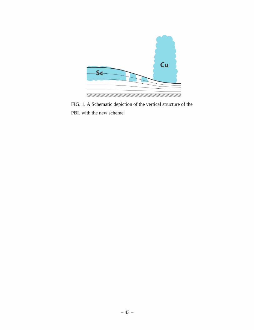
– 43 –

FIG. 1. A Schematic depiction of the vertical structure of the

PBL with the new scheme.

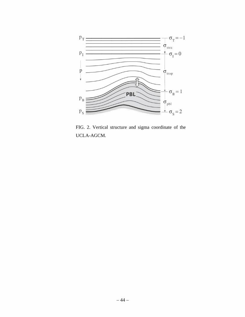
– 44 –

FIG. 2. Vertical structure and sigma coordinate of the

UCLA-AGCM.

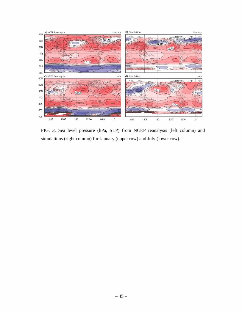
– 45 –

FIG. 3. Sea level pressure (hPa, SLP) from NCEP reanalysis (left column) and

simulations (right column) for January (upper row) and July (lower row).

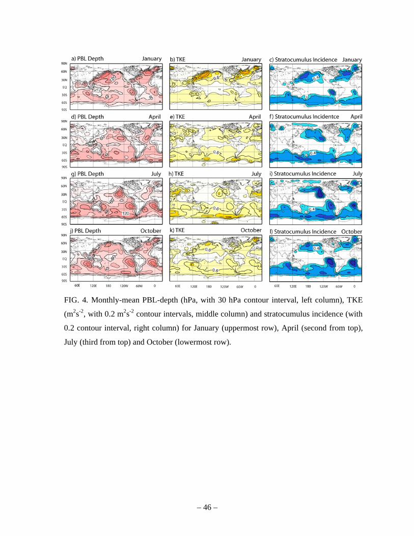
– 46 –

FIG. 4. Monthly-mean PBL-depth (hPa, with 30 hPa contour interval, left column), TKE

(m2s

-2, with 0.2 m

2s

-2 contour intervals, middle column) and stratocumulus incidence (with

0.2 contour interval, right column) for January (uppermost row), April (second from top),

July (third from top) and October (lowermost row).

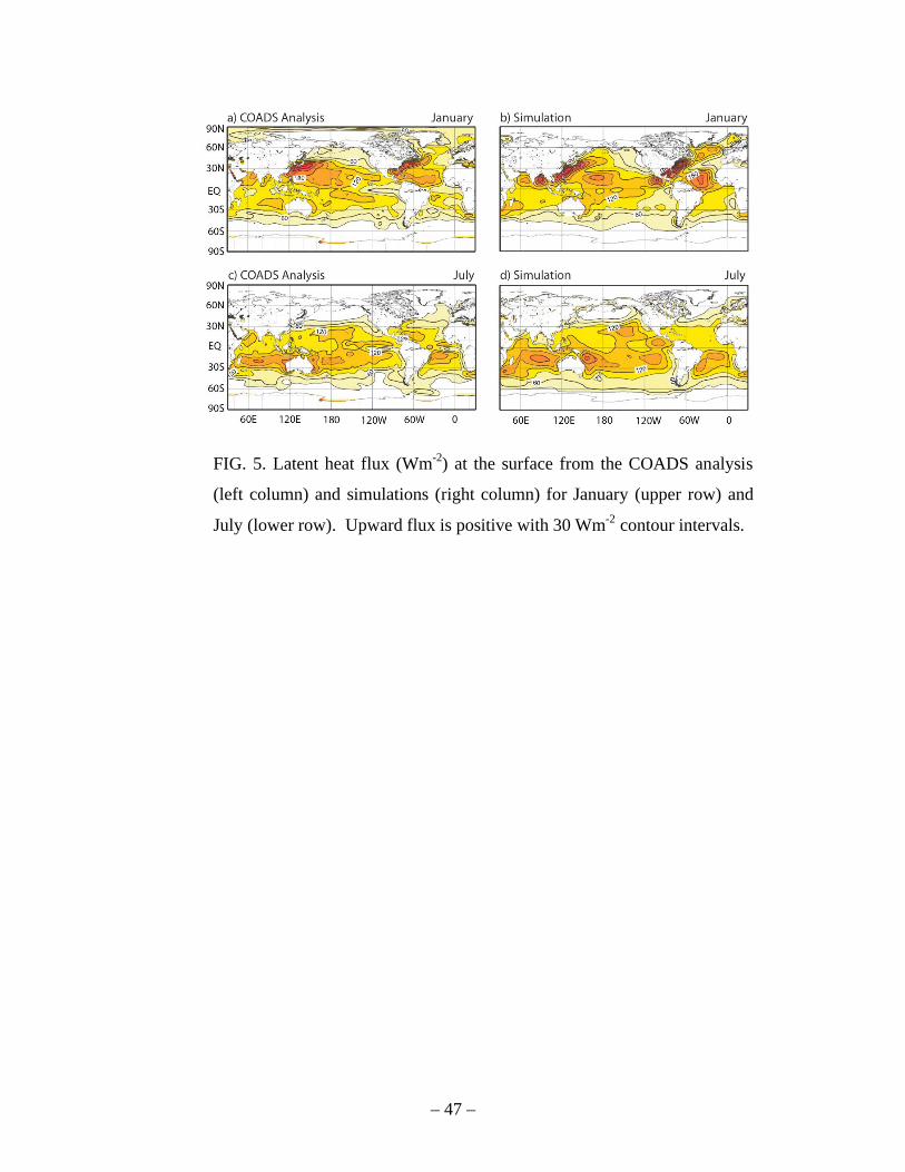
– 47 –

FIG. 5. Latent heat flux (Wm-2

) at the surface from the COADS analysis

(left column) and simulations (right column) for January (upper row) and

July (lower row). Upward flux is positive with 30 Wm-2

contour intervals.

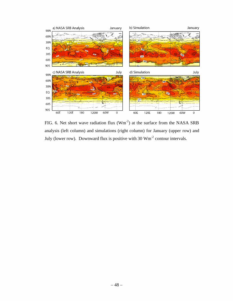
– 48 –

FIG. 6. Net short wave radiation flux (Wm-2

) at the surface from the NASA SRB

analysis (left column) and simulations (right column) for January (upper row) and

July (lower row). Downward flux is positive with 30 Wm-2

contour intervals.

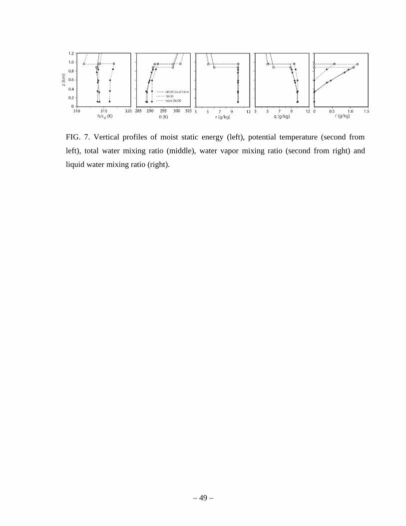
– 49 –

FIG. 7. Vertical profiles of moist static energy (left), potential temperature (second from

left), total water mixing ratio (middle), water vapor mixing ratio (second from right) and

liquid water mixing ratio (right).

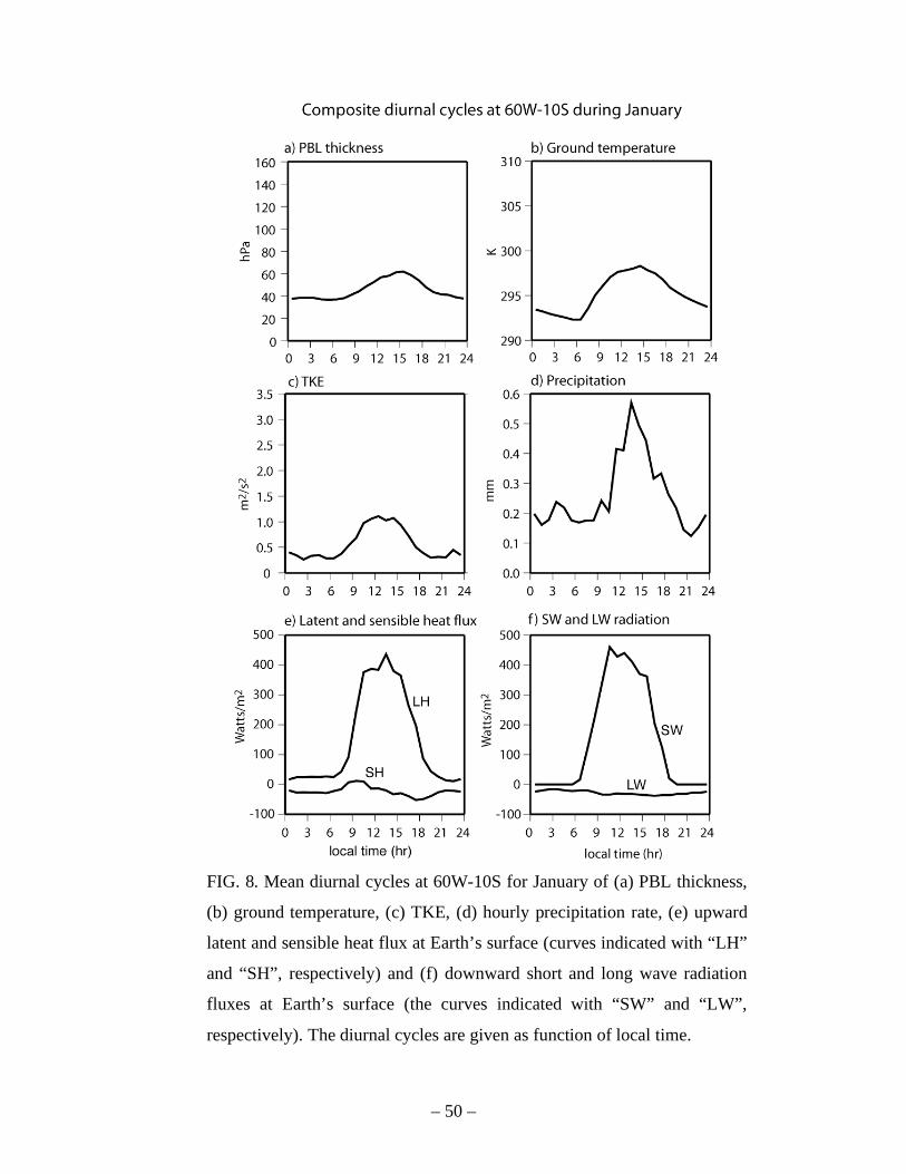
– 50 –

FIG. 8. Mean diurnal cycles at 60W-10S for January of (a) PBL thickness,

(b) ground temperature, (c) TKE, (d) hourly precipitation rate, (e) upward

latent and sensible heat flux at Earth’s surface (curves indicated with “LH”

and “SH”, respectively) and (f) downward short and long wave radiation

fluxes at Earth’s surface (the curves indicated with “SW” and “LW”,

respectively). The diurnal cycles are given as function of local time.

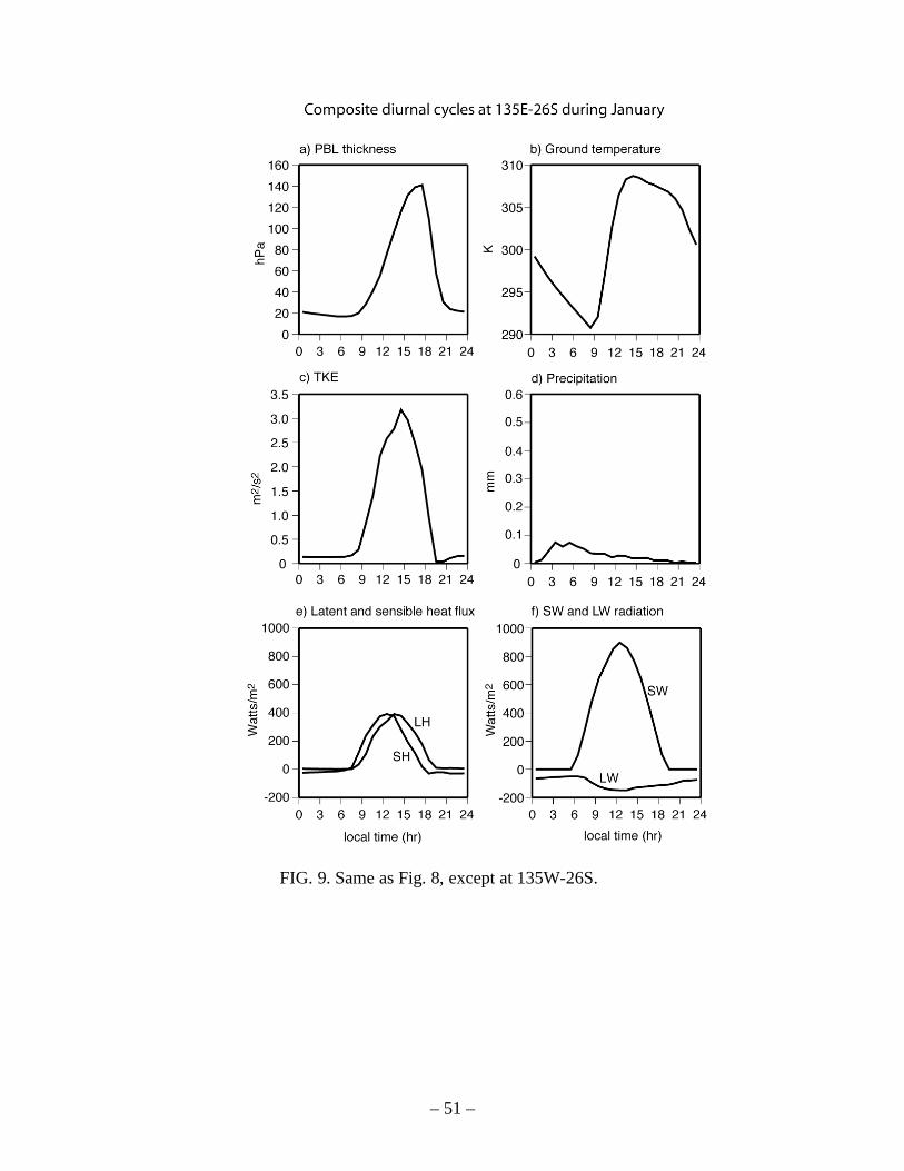
– 51 –

FIG. 9. Same as Fig. 8, except at 135W-26S.

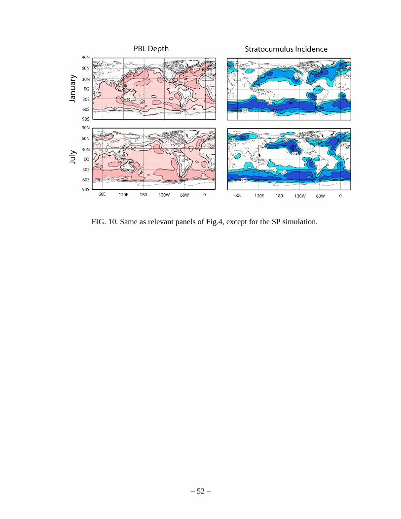
– 52 –

FIG. 10. Same as relevant panels of Fig.4, except for the SP simulation.

– 53 –

FIG. 11. Same as Fig.5, except for the SP simulation.

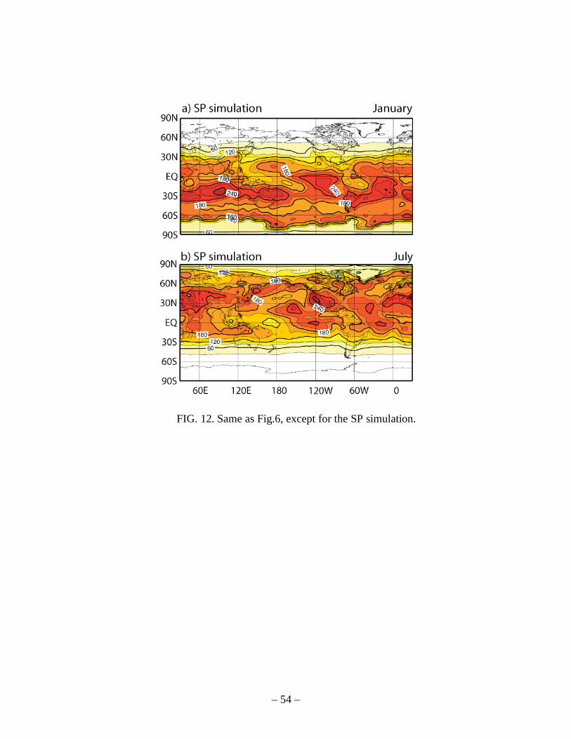
– 54 –

FIG. 12. Same as Fig.6, except for the SP simulation.

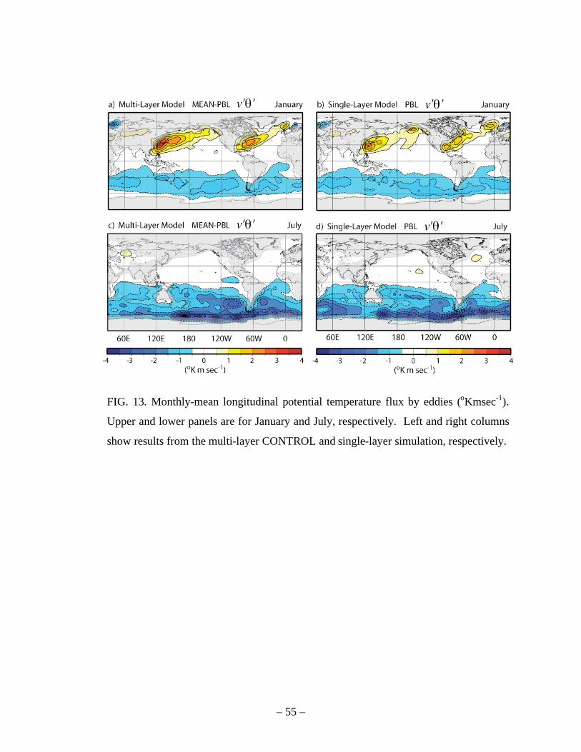
– 55 –

FIG. 13. Monthly-mean longitudinal potential temperature flux by eddies (oKmsec

-1).

Upper and lower panels are for January and July, respectively. Left and right columns

show results from the multi-layer CONTROL and single-layer simulation, respectively.

– 56 –

FIG. 14. Monthly-mean TKE (upper panel), PBL thickness (hPa, middle panel) and

stratus incidence (lower panel) from the simulation with no radiative cooling effect in

TKE and entrainment (NR1, left column) and difference between NR1 and Control (Fig.

4) simulations (right column).

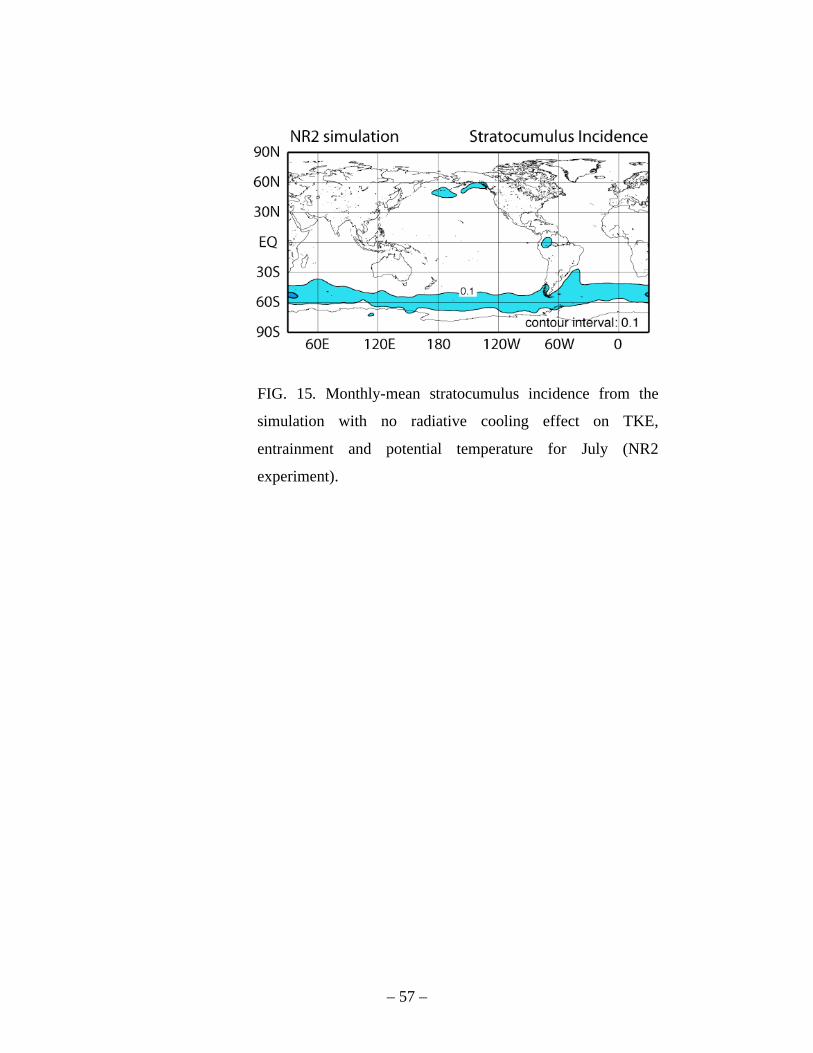
– 57 –

FIG. 15. Monthly-mean stratocumulus incidence from the

simulation with no radiative cooling effect on TKE,

entrainment and potential temperature for July (NR2

experiment).

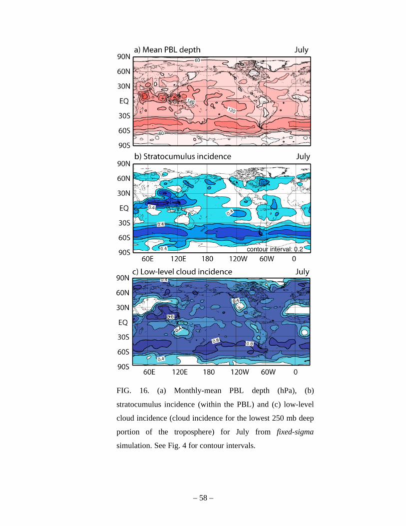
– 58 –

FIG. 16. (a) Monthly-mean PBL depth (hPa), (b)

stratocumulus incidence (within the PBL) and (c) low-level

cloud incidence (cloud incidence for the lowest 250 mb deep

portion of the troposphere) for July from fixed-sigma

simulation. See Fig. 4 for contour intervals.